Modeling and Experimental Parameter Estimation of a Refrigerator/Freezer System
R. N. Reeves, C. W. Bullard and R. R. Crawford
ACRCTR-09
For additional information:
Air Conditioning and Refrigeration Center University of Illinois Mechanical & Industrial Engineering Dept. 1206 West Green Street Urbana,IL 61801
(217) 333-3115
January 1992
Prepared as part of ACRC Project 12 Analysis of Refrigerator-Freezer Systems
C. W. Bullard, Principal Investigator
The Air Conditioning and Refrigeration Center was founded in 1988 with a grant from the estate of Richard W. Kritzer, the founder of Peerless of America Inc. A State of Illinois Technology Challenge Grant helped build the laboratory facilities. The ACRC receives continuing support from the Richard W. Kritzer Endowment and the National Science Foundation. Thefollowing organizations have also become sponsors of the Center.
Acustar Division of Chrysler Allied-Signal, Inc. Amana Refrigeration, Inc. Brazeway, Inc. Carrier Corporation Caterpillar, Inc. E. I. du Pont de Nemours & Co. Electric Power Research Institute Ford Motor Company Frigidaire Company General Electric Company Harrison Division of GM ICI Americas, Inc. Modine Manufacturing Co. Peerless of America, Inc. Environmental Protection Agency U. S. Anny CERL Whirlpool Corporation
For additional iriformation:
Air Conditioning & Refrigeration Center Mechanical & Industrial Engineering Dept. University of Illinois 1206 West Green Street Urbana IL 61801
2173333115
MODELING AND EXPERIMENTAL PARAMETER ESTIMATION OF A REFRIGERA TOR/FREEZER SYSTEM
Ronald Nicholas Reeves, M.S.
Department of Mechanical and Industrial Engineering University of Illinois at Urbana-Champaign, 1992.
ABSTRACf
This paper examines a set of simple equations describing a domestic refrigerator/freezer
system and suggests several modeling improvements, based on experimental results. The
experimental setup is described and limitations in the accuracy of the sensors is examined.
Data are compared to predictions from a fIrst generation model. Changes are made in the
model to improve representations of heat exchanger geometry and flow regimes, and air
side energy equations. The experimental data are re-examined in order to quantify the
accuracy gained as model complexity was increased. For both models, parameters are
estimated from the data using nonlinear least squares parameter estimation methods,
implemented using multivariate and univariate optimization algorithms.
iii
Table of Contents
Chapter Page
List of Figures ...................................................................................... vii
1. Introduction..................................................................................... 1 Purpose .................................................................................... 1 Refrigerator Energy Use.. . . .. .. .. . .. . . .. . ... . .. . . .. . . .. . . .. . .. . . .. . . .. . . . . . .. . . . . . . . . . .. 1 The Ozone Problem and Alternate Refrigerants. . .. . . .. . . . .. . . .. . . . . . . . .. . . . .. . . . . . . .. 2 Improved Simulation Models ............................................................ 2
2. Literature Review. . . . . . . . . . . . . . . . . . . . . . . . . . . . . . . . . . . . . . . . . . . . . . . . . . . . . . . . . . . . . . . . . . . . . . . . . . . . . . . 4 Heat Exchanger Modeling. .. . . . . . . .. . . .. . .. . . .. . . .. . . .. ... . . . . . . .. . . .. . .. . . . . . . .. . . .. . .. 4 Evaporator. .. . . .. . .. . . .. . .. . . .. . . . . . .. . . .. . .. . . .. . .. . ... . .. .. .. . ... . .. . ... . . . . . .. . .. . . .. . .. 5 Condenser ................................................................................. 7 Capillary Tube/Suction Line Heat Exchanger.. . . . .. . ... . . .. . . . .. . . .. . . .. . . . .. . . .. . . .. 7 Compressor ................................................................................ 9 System Level Analysis ................................................................... 10
3. Experimental Setup ............................................................................. 13 Environmental Test Chamber ............................................................ 13 Refrigerant Temperature Measurement ................................................. 14 Refrigerant Pressure Measurement ..................................................... 14 Air Side Temperature Measurement .................................................... 15 System Power Measurement ............................................................ 15 Mass Flow Rate Measurement .......................................................... 16 Data Acquisition System ................................................................. 16 Test Protocol .............................................................................. 17
4. Parameter Estimation- Evaporator ........................................................... 19 Determining Evaporator Heat Load (Qevap) ........................................... 19 Air Side Energy Balance ................................................................. 21 Estimation of Heat Transfer Parameters ................................................ 24 Predicting Evaporator Performance ..................................................... 26
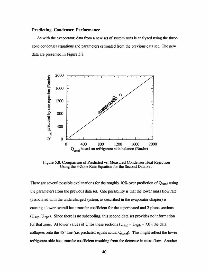
5. Parameter Estimation- Condenser ............................................................ 30 Determining Condenser Heat Rejection (Qcond) ..................................... .30 Air Side Energy Balance ................................................................. 31 Estimation of Heat Transfer Parameters ............................................... .36 Predicting Condenser Performance ..................................................... 40
6. Parameter Estimation- Compressor .......................................................... 42 Determining Compressor Heat Rejection (Qcomp) .................................. .42 Determining the Effective Heat Transfer Coefficient ................................ .42
7. Parameter Estimation- Suction Line Heat Exchanger ..................................... .45 Detennining Interchanger Heat Transfer (Qint) ...................................... .45 Determining Interchanger Effectiveness ............................................... .46 Estimating Interchanger Heat Transfer Coefficient (U Aint) ......................... 48 Comparison of eint and UAint .......................................................... 49
8. Modeling- Overall System .................................................................... 51 ADL Version .............................................................................. 51 ACRC Versions ........................................................................... 52
9. Modeling- Evaporator ......................................................................... 53
v
ADL Version .............................................................................. 53 ACRCI Version ........................................................................... 54 ACRC2 Version ........................................................................... 55
10. Modeling- Condenser ........................................................................ 56 ADL Version .............................................................................. 56 ACRCI Version ........................................................................... 58 ACRC2 Version ........................................................................... 58
11. Modeling- Compressor ...................................................................... 61 ADL Version .............................................................................. 61 ACRC 1 Version ........................................................................... 62 ACRC2 Version ........................................................................... 63
12. Modeling- Suction Line Heat Exchanger .................................................. 64 AD L Version .............................................................................. 64 ACRC Versions ........................................................................... 65
13. Conclusions and Recommendations ........................................................ 66 Conclusions ............................................................................... 66 Recommendations for Future Research ................................................ 67
References .......................................................................................... 70
Appendix A: Cabinet Heat Load vs. Refrigerant Side Balances ............................. 73 Choice of Refrigerant Mass Flow Rate ................................................. 73 Energy Balances .......................................................................... 7 4
Appendix B: Heat Exchanger Geometries ...................................................... 77 Evaporator ................................................................................. 77 Condenser ................................................................................. 7 8
Appendix C: Turbine Flow Meter ............................................................... 80 Hardware and Instrumentation .......................................................... 80 Meter Calibration .......................................................................... 81 Density Correction ........................................................................ 82
Appendix D: Instrumentation Blocks ........................................................... 84 Hardware .................................................................................. 84 Thermocouple Installation ............................................................... 85 Pressure Connections .................................................................... 86
vi
List of Figures
Figure Page
3.1. Environmental Test Chamber ............................................................... 13 4.1. Heat Transfer Paths into Refrigerator and Freezer Cabinets ............................ 19 4.2. Refrigerant Side Energy Balance on the Evaporator .................................... 20 4.3. Comparison of Predicted vs. Measured Evaporator Air Inlet Temperatures .......... 23 4.4. Comparison of Predicted vs. Measured Evaporator Load Using the I-Zone
Rate Equation ................................................................................. 25 4.5. Comparison of Predicted vs. Measured Evaporator Load Using the 2-Zone
Rate Equation ................................................................................. 26 4.6. Comparison of Predicted vs. Measured Evaporator Load Using the 2-Zone
Rate Equation for a New Data Set ......................................................... 27 4.7. Comparison of Predicted vs. Measured Evaporator Air Inlet Temperature for
the Second Data Set .......................................................................... 28 5.1. Refrigerant Side Energy Balance on the Evaporator ..................................... 30 5.2. Condenser Air Flow Path ................................................................... 31 5.3. Predicted vs. Measured Air Inlet Temperatures ......................................... .32 5.4. Predicted vs. Measured Compressor Air Temperatures ................................. 33 5.5. Estimated Condenser Fan Air Flow as a Function of Fraction of Air Leaving
Behind the Compressor ..................................................................... 35 5.6. Comparison of Predicted vs. Measured Condenser Heat Rejection Using the 2-
Zone Rate Equation .......................................................................... 37 5.7. Comparison of Predicted vs. Measured Condenser Heat Rejection Using the 3-
Zone Rate Equation .......................................................................... 39 5.8. Comparison of Predicted vs. Measured Condenser Heat Rejection Using the 3-
Zone Rate Equation for the Second Data Set ............................................ .40 6.1. Compressor Control Volume and Energy Paths ......................................... .42 6.2. Estimation of Compressor Heat Transfer ................................................ .43 6.2. Estimation of Compressor Heat Transfer with the Second Data Set ................... 44 7.1. Interchanger Energy Balance .............................................................. .45 7.2. Estimation of Interchanger Effectiveness ................................................. .47 7.3. Predicted vs. Measured Compressor Inlet Temperature (eint = const.) .............. .48 7.4. Predicted vs. Measured Compressor Inlet Temperature (UAint = const.) ........... .49 9.1. Forced Convection Evaporator and Refrigerant Loop .................................. .53 10.1. Forced Convection Condenser and Refrigerant Loop .................................. 56 11.1. Compressor System ........................................................................ 61 12.1. Suction Line Heat Exchanger System .................................................... 64 A.l. Comparison of Mass Flow Rate from Compressor Map and Turbine ................ 73 A.2. Energy Balance on the Evaporator ......................................................... 75 A.3. Location of Condenser Exit Instrumentation Block and Flow Meter .................. 76 B.l. Evaporator Geometry ....................................................................... 77 B.2. Condenser Geometry ........................................................................ 78 C.l. Turbine Flow Meter and Signal Conditioning Components ............................ 80 C.2. Plot of Turbine Output vs. Measured, Coriolis Mass Flow Rate ...................... 81 C.3. Turbine Mass Flow Data Corrected For Density ......................................... 83 D.l. Instrumentation Block With 45° Bend ..................................................... 84 D.2. Instrumentation Block With 90° Bend ..................................................... 85
vii
Purpose
Chapter 1
Introduction
The purpose of this research project is: 1) to identify existing refrigerator/freezer
simulation models in public domain; 2) instrument a refrigerator as nonintrusively as
possible to obtain data to validate an existing steady state model; 3) make improvements in
the model as warranted by the experimental results. Both the accuracy and generality (with
respect to geometry and refrigerant choice) of existing and improved models will be
addressed.
Refrigerator Energy Use
In 1982 the Arthur D. Little Corporation (ADL, 1982) developed a refrigerator and
freezer simulation model under contract for the Department of Energy (DOE). The model
was used by DOE to assist in the determination of energy standards for refrigerators,
refrigerator/freezers, and freezers. Several different cabinet configurations were possible
with the ADL model, including; top-mount or bottom-mount freezers, side-by-side
refrigerator/freezers, and single-door units. Also, the model allowed for various
configurations of evaporators and condensers, including; free convection, forced
convection, and wall condensers, along with free convection, forced convection, and wall
panel evaporators.
The ADL model is the latest computer simulation model in the public domain that was
designed specifically for refrigerators/freezers, and remains DOE's best tool for setting
future refrigerator energy standards.
1
The Ozone Problem and Alternate Refrigerants
Recent evidence (Science v. 254 no. 5032, 1991) indicates that the stratospheric ozone
depletion problem may be significantly worse than estimated only a few years ago. One of
the suspected causes of ozone depletion is CFC-12 (CCI2F2), which is used as a working
fluid in the vapor compression cycle of the refrigerators and freezers. The challenge of
eliminating CFC-12 completely by the end of the century has appliance manufacturers
seeking information that can assist in quantifying the refrigerator performance changes
associated with changes to alternate refrigerants.
Improved Simulation Models
The relative success of the ADL model in the past is due, in part, to two things. First,
the refrigerant used in the simulation has always been CFC-12, for which there exists a
large variety of performance and property data in the literature. Second, the model is based
of refrigerator performance at test conditions (usually a 90°F test chamber). At these test
conditions, simplifying ADL assumptions (5°F of condenser subcooling and no evaporator
superheat, for example) are fairly valid. When switching to an alternative refrigerant, or at
a different operating condition, however, these assumptions begin to break down.
Thus, an urgent need for an improved simulation model exists. With this need in mind,
this research is aimed at developing an improved simulation model to:
• quantify performance tradeoffs;
• analyze improved system configurations; and
• optimize system performance.
This research project will address these issues with a well instrumented, top-mount
refrigerator-freezer. The data presented herein is for CFC-12, as a baseline for comparison
with existing data an models.
The results of this research are presented in the following chapters. Chapter 2 provides
a review of the literature dealing with both the components and the system simulation.
2
Chapter 3 outlines the experimental setup and the instrumentation used in obtaining all of
the data. Chapters 4 through 7 deal with parameter estimation on a component by
component basis. Chapter 8 provides a discussion of modeling on the system level, while
Chapters 9 through 12 present the modeling at the component level. Finally, Chapter 13
concludes with a summary and list of recommendations for future research.
3
Chapter 2
Literature Review
The goal of the literature review is to identify previous work that will be useful in
refrigerator/freezer modeling. The existing literature related to this research is divided into
two main areas; component and system level analyses. The component literature provides
descriptions and equations describing each of the system components. The system level
literature addresses issues such as alternative refrigerants, refrigerant charge, transient
analysis, etc. In this review, papers and reports not dealing directly with the component
level will be grouped into the system analysis section.
Heat Exchanger Modeling
A basic review of the heat transfer relations necessary for heat exchanger modeling is
obtained from a text on refrigeration and air conditioning (Stoecker, 1982). Stoecker's text
reviews the basic relations for conductance (VA), overall heat transfer coefficient (V), and
ways of evaluating these quantities using resistance networks and convective heat transfer
coefficients.
Several analytical solutions for calculating heat transfer coefficients are presented in a
report that summarizes the Oak Ridge National Lab (ORNL) heat pump model (Rice,
1983). Relations are included for both air side and refrigerant side heat transfer
coefficients. The relations are closed form solutions of integrals presented in the write-up.
This model also treats mass transfer onto a coil as a function of humidity ratio.
A review of a text specifically written for heat exchanger design (Kays & London,
1984) provides a wealth of information for heat exchanger modeling using the E-NTU
method. Analytical solutions for heat exchanger effectiveness are provided for many
different geometries and configurations. Also, methods are reviewed for calculating these
parameters analytically from basic relations for geometries that are not included in the text.
4
Heat transfer augmentation/degradation due to oil concentration is examined by Eckels
and Pate for in-tube evaporation and condensation of refrigerant-lubricant mixtures (Eckels,
1991). Experimental data is presented for different oil concentrations (0, 1.2,2.5, and
5.4%) in both CFC-12 (naphthenic oil) and HFC-134a (PAG oil). Overall pressure drop
and heat transfer coefficient data are presented graphically as a function of oil concentration
for both refrigerants.
A much more detailed set of data showing how heat transfer pressure drops vary with
quality, mass flux, heat flux, and other parameters are presented by Wattelet, Chato,
Jabardo, Panek, and Renie (Wattelet, 1991). The two-phase heat transfer tests are
conducted for evaporation, with and without various oils. The refrigerants tested are CFC-
12 and HFC-134a with an inlet quality of 20% and saturation temperatures between 4.4
and 11.1°C. A similar study was conducted by Bonhomme, Chato, Hinde, and Mainland
for condensation parameters (Bonhomme, 1991).
Evaporator
One method of modeling an evaporator is presented by Parise (1986), who assumes a
constant overall heat transfer coefficient, UEV, for both the saturated and superheated
sections of the evaporator. Model inputs include the inlet air temperature, the mass flow
rate and heat capacity of dry air, and the evaporator area. The relations presented give the
total amount of heat transferred by the evaporator.
In another article, Kayansayan uses a "Mean Heat Flux Concept" in evaporator design.
This method is used to determine the area of an evaporator if the refrigerant circuit
configuration, the refrigerant, the desired amount of heat transfer, and the working
conditions are all known. The algorithm accounts for temperature differences between the
fluid and the tube wall as the air moving over the evaporator is cooled. The method is
similar to the LMTD method. The LMID method is based on a mean temperature and
5
Kayansayan's method is based on a mean heat flux. Since no experimental data are
presented, it is difficult to evaluate this method.
Finned tube evaporator relations are presented in a paper by O'Neill and Crawford
(O'Neill, 1989). Although the paper deals mainly with heat exchanger optimization,
conductance relations are presented as a function of air side, refrigerant side, tube, and
tube/fin contact resistances. Also, Wilson plots are presented that show the relationship
between conductance and refrigerant flow rate for a refrigerator evaporator with various
fine spacings (0, 1.25, 2.5, and 5 fins per inch).
Air side heat transfer correlations are presented for different fin configurations by
Beecher and Fagan (Beecher, 1987). The various configurations include variations in fin
and tube spacings. The data is presented graphically, along with curve fits giving empirical
expressions for Nu as a function of Gz and other parameters of interest. The usefulness of
this data is questionable since the reference fin spacing for this study is 0.077 inches, low
for refrigerator evaporators.
A similar study is presented by Webb (Webb, 1990) for flat and wavy plate fin-and-tube
geometries. Data for both flat and wavy plates is presented for various fm spacings
(0.056,0.077,0.094,0.110, and 0.161 inches). Variations in the space between adjacent
tubes as well as the space between the tube rows are also examined.
Domanski presents the results of a study of non-uniform air distribution over an
evaporator (Domanski, 1991). A tube-by tube method is used so that complex refrigerant
circuitry could be examined. Heat transfer parameters are calculated for different air
velocity proflles. Also, experimental data (including measured velocity proflles) are used
to validate the model. The predictions are within 8.2% of the measured data.
The effect of frosting on evaporator performance is presented by Rite (1990a and
1990b). The test evaporator is a typical aluminum plate and fin-and-tube unit with a fm
spacing of 5 fins per inch. Air side pressure drop, conductance (VA), and frosting rate is
6
presented for different relative humidities as a function of time (as frost builds up on the
evaporator).
Condenser
Three-zone modeling of a mobile air conditioning condenser is examined by Kempiak
(1992). A constant heat transfer coefficient is assumed for each of the three zones
(desuperheating, two-phase, and subcooling). Refrigerant mass flow rate, and air flow
rate are experimentally varied to estimate the coefficients for the heat transfer correlations
for a finned tube condenser.
Condensation heat transfer is examined inside tubes by Nitheanandan et.al. (1990).
This two-phase study looks at the different flow regimes for both a low and high mass flux
case. Heat transfer correlations are derived from experimental data for each of the regions
of two-phase flow. The scatter in the data is significant, making general correlations
difficult. The trends, however, are useful in examining different flow patterns and in
estimating overall condenser heat transfer coefficients.
Capillary Tube/Suction Line Heat Exchanger
Pate and Tree (1984a) summarize the parameters of interest and the associated analysis
of a capillary tube/suction line heat exchanger. Tube diameter ratios ranging from eight to
ten are typical for domestic refrigerators. The soldered tubes are essentially a counterflow
heat exchanger, conducting heat from the capillary tube to the suction line. Although the
construction of the device is simple, the flow phenomena are complex. From the inlet to
exit, the capillary tube contains refrigerant experiencing adiabatic single-phase flow, single
phase flow with heat transfer, two-phase flow with heat transfer, adiabatic two-phase flow,
and two-phase choked flow at the exit plane.
Pate and Tree have also developed a linear quality model for analyzing the capillary
tube/suction line heat exchanger (Pate, 1984b). This model assumes a linear profile of
7
quality along the length of the two-phase section of the capillary tube. The model is
computationally an initial value marching problem. The initial condition is the flash point
(calculated in another routine). The algorithm solves four unknowns at each step location
along the capillary tube; distance from flash point (Z), quality (x), temperature of the
suction line fluid (T s), and capillary tube wall temperature (T w). The algorithm uses an
energy and momentum equation.
Schulz (1985) reviews the research on adiabatic capillary tubes noting that the flow rate
of refrigerant through a capillary tube does not continue to increase with increasing
pressure difference, but reaches a maximum choked value at a certain pressure drop.
Goldstein presents an iterative approach to modeling flashing flow in adiabatic capillary
tubes (Goldstein, 1981). This mathematical approach can model flashing flow from a
liquid or two-phase inlet to a liquid or two-phase outlet. Goldstein fixes the inlet and outlet
pressures of the tube and the model fmds the right combination of compressor mass flow
rate and pressure drop to satisfy the system. He notes that the two-phase mixture may be
compressible, such that its sonic velocity must be evaluated to find the critical flow rate.
This technique breaks the tube into many segments for sequential analysis.
Li, Lin and Chen present a numerical method of modeling non-equilibrium refrigerant
flow through adiabatic capillary tubes (Li, 1990). Their approach involves several
differential conservation equations (energy, momentum, mixture mass, and vapor mass).
These equations, along with frictional pressure drop coefficients and equations describing
the mass transfer due to vaporization are combined with thermodynamic relations to yield a
complete set, where the number of equations equals the number of unknowns. The
differential equations are solved using Runge-Kutta integration. The data presented is in
good agreement with the model in predicting pressure and quality as a function of position
along the capillary tube.
8
Compressor
A basic analysis of reciprocating compressor perfonnance and modeling is presented by
Stoecker and Jones in their Refrigeration and Air Conditioning text (Stoecker, 1982). The
authors present two techniques for compressor modeling; using a bi-quadratic least squares
fit and using volumetric efficiency analysis. The volumetric efficiency analysis appears to
be a better method for modeling a compressor since it relies on physical parameters that can
be measured and used to predict compressor perfonnance. Also, a "compressor efficiency"
tenn is introduced to correct clearance volume efficiency for real system losses, so that
actual volumetric efficiency can be obtained The bi-quadratic method is simply a least
squares curve fit of the desired compressor perfonnance parameter (mass flow rate, power
consumption, etc.) with respect to the condensing and evaporating temperatures (i.e.
saturation pressures). This curve fit is a result of a set of experimentally measured
compressor perfonnance data.
A more complex compressor analysis is presented by Rice (1983) in a document
describing the Oak Ridge National Lab heat pump model. Internal energy balances are
used to model internal efficiency and heat loss values for a reciprocating compressor. This
means that the user is required to specify a variety of physical compressor parameters,
including total displacement, clearance volume ratio, motor speed, shaft power, motor
efficiency, mechanical efficiency, and isentropic compression efficiency. Energy balance
equations and system defining equations are simultaneously solved to yield perfonnance
parameters, such as refrigerant mass flow rate, compressor can losses, etc.
In a paper published by Kent, the validity of using a polytropic gas coefficient is
examined (Kent, 1984). The results of the research indicate that the polytropic gas
coefficient, N, is not constant during the entire compression cycle. In fact, experimental
data indicates that N can vary as much as 20% in some instances. It was postulated that the
variation may be due to irreversible effects such as friction, heat transfer, and pressure
9
pulsations in the cylinders and valves. Reasonable lower and upper bounds for N are for
an isothennal compression (N=I) and an adiabatic process (N=1.4 for a diatomic gas).
In a related study, Rottger and Kruse (Rottger, 1976) examine the application of perfect
gas law relationships to the compression process. That show perfonnance deviations as
great as 10% when using ideal gas relations for the compressor calculations. This
demonstrates the importance of accounting for real gas behavior in compressor simulation
models.
System Level Analysis
The Department of Energy (DOE) refrigerator/freezer efficiency model is examined in an
article by Abramson, Turiel, and Heydari (1990). The model was developed by Arthur D.
Little, Inc. (ADL) under a DOE contract in 1982. The authors summarize the governing
equations used by the model, the model nomenclature, and the various refrigerator-freezer
configurations that the model is designed to simulate. In this particular paper, the model is
used to simulate a top mount, 18 cubic foot refrigerator/freezer. Performance is evaluated
by graphically comparing the yearly energy consumption as a function of wall thickness,
the UA of the evaporator, and the UA of the condenser.
Chen and Lin (1991) outline a method for simulating the dynamics of a
refrigerator/freezer system. Their first step is to define the differential equations for each of
the components, derived from physical laws of mass and energy conservation. Next, the
differential equations are organized in a fonn such that their solution would yield the results
in the desired fonn (i.e. in tenns of enthalpy, temperature, pressure, etc.). Finally, the
equations are reduced to numerical fonn and a time marching Euler method is used to
simulate the system. The authors use the technique to predict refrigerant and air side
temperatures and pressures at desired locations. Experimental data collected at these
locations shows relatively good agreement with the model predictions.
10
A perfonnance simulation of a single-evaporator domestic refrigerator is reviewed by
Jung and Radennacher (Jung, 1991). The authors used the CYCLE7 model (developed by
McLinden and Radennacher, 1987) to compare the cycle efficiency for several pure and
mixed refrigerants. The heat exchangers (evaporator and condenser) are modeled using the
LMID method. Pressure drop in the heat exchangers is modeled as a function of heat
transfer in each of the regions (subcooled, two-phase, and superheated). The authors
discuss two methods of solving the system of equations and unknowns describing the
refrigerator system; successive substitution and simultaneous solution (Newton-Raphson).
The successive substitution method involves an iterative approach, where the equations
need to be carefully ordered, and a flow chart constructed for the solution methodology.
The Newton-Raphson technique uses matrix inversion techniques to simultaneously solve
an NxN system of equations and unknowns. Jung and Radennacher report a 20-25%
longer run time for the successive substitution method compared to the Newton-Raphson
for the CYCLE7 equations (using a 80386/20 MHz PC with an 80387/20 MHz math
coprocessor). The COP, volumetric capacity, and pressure ratio are presented for 15 pure
refrigerants and mixtures of R32/R142b and R22/R142b.
Cecchini and Marchal present a model that can be used to simulate refrigeration and air
conditioning equipment (Cecchini, 1991). The model is based on experimental data, used
to estimate perfonnance parameters based on a "few" testing points. The compressor is
modeled using polytropic exponents and ideal gas law equations. The heat exchangers are
modeled assuming that the heat transfer rate is a linear function of refrigerant and air inlet
temperature difference. The expansion device is modeled using ideal gas relations, based
on thennodynamic functions with respect to pressure drop. The entire system is modeled
with eleven equations and 11 unknowns. The authors claim that the model predicts
measured performance within 10%, based on pressure and temperature measured at the
four testing points.
11
The effect of refrigerant charge on heat pump perfonnance is examined by Damasceno,
Domanski, Rooke, and Goldschmidt (Damasceno, 1991). The authors present measured
and predicted perfonnance as a function of refrigerant charge for heat pumps in both the
heating and cooling modes. The predicted performance is based on the Lockhart-Martinelli
void-fraction model. For this model, void fraction is an input, and can be calculated using
different methods. The authors limit themselves to the Zivi, Tandon, and Hugbmark
expressions for calculating two-phase void fraction. Internal volume calculations are
performed to facilitate refrigerant inventory modeling. Finally, these equations are
combined into a heat pump simulation model, HPSIM, in a two step procedure which
yields HPSIMI (containing modifications to coil circuitry mapping and internal volume
calculations) and HPSIM2 (including all of the void fraction equations). Using HPSIM2,
the trends in cooling capacity are predicted fairly well. The trends in heating capacity,
however, do not show very good agreement.
The perfonnance of ozone-safe alternative refrigerants is examined by Sand, Vineyard,
and Nowak (Sand, 1990) in a breadboard vapor-compression circuit designed to simulate a
heat pump. The authors evaluate the performance of several ozone-unsafe refrigerants and
compare the results with candidate ozone-safe alternative refrigerant replacements. The
parameters used in the comparison include; compression ratio, net heating effect, net
cooling effect, refrigerant circulation rate, and coefficient of performance (for both heating
and cooling). The results of the experimental study are summarized in several tables in the
report.
12
Chapter 3
Experimental Setup
Environmental Test Chamber
Prior to the initiation of refrigerator testing, an environmental test chamber was designed
and constructed by another graduate student Figure 3.1 shows the test chamber with the
associated air-conditioning unit and duct work.
R-34 Insulation & Vapor Barrier
Test Refrigerator
Supply Air Diffuser Plenum
D -
+ Return
R-7 Insulated Floor Temperature Sensor
Figure 3.1. Environmental Test Chamber
Supply
Electric Reheat
+ Packaged NCUnit
The test chamber is used to control the ambient temperature surrounding the refrigerator.
This control is achieved with a PID temperature controller (used in the proportional and
integral mode), which pulses power to a 7.6 kW electric reheat coil. The air-conditioning
portion of the system (18,000 Btu/h rated capacity) is run at all times, and the only control
is through the reheat coil.
13
Refrigerant Temperature Measurement
Refrigerant temperature is measured with "Type T" (copper-constantan) immersion
thermocouples. The thermocouples are contained in a sixteenth inch 304 stainless steel
sheath, with the thermocouple bead at the tip. This model of immersion thermocouple is
not grounded to the sheath, as it is with some models. The thermocouples are placed in the
refrigerant stream using brass instrumentation blocks, as discussed in Appendix D. To
minimize axial heat conduction errors, the tip of the immersion thermocouple is placed as
far into the refrigerant stream as possible. This distance is limited by the uncertainty that
the tip may contact the tube wall, introducing significant error. The manufacturer claims an
accuracy of ±D. 5°C (±D.9°F) for any "Type T" thermocouple (OMEGA, 1989).
Refrigerant Pressure Measurement
Two types of pressure transducers are used to determine the pressures at the five points
in the system between each of the components. Two gage pressure transducers are used to
measure the high pressure (compressor exit) and low pressure (evaporator outlet) parts of
the system. The manufacturer claims ±O.13% Full Scale accuracy. This translates to
±D. 13 psig for the evaporator outlet (0-100 psig range) and ±O.33 psig for the compressor
outlet (0-250 psig range). Three differential pressure transducers are used to determine the
pressure drop across three of the components; the suction line, the condenser, and the
evaporator. The manufacturer claims ±D. 1 1 % Full Scale accuracy for the differential
pressure transducers. This translates to ±D.06 psi for all transducers (0-±25 psid range).
With these five pressure transducers, the five pressures between the system components
are measured directly or can be calculated from the pressure drops measured with the
differential pressure transducers. See Appendix D for further information about how the
pressure taps are incorporated into the instrumentation blocks.
14
Air Side Temperature Measurement
All of the air side thennocouples were made by soldering "Type T" thennocouple wire,
purchased in large rolls. Two different types were fabricated, depending on the desired
measurements. The refrigerator and freezer cabinets contain four and two independent
thennocouples, respectively. By monitoring the temperatures at different locations in the
cabinets, the level of stratification can be detennined. The other type, thennocouple arrays,
are used everywhere else for air temperature measurements. The arrays are a collection of
several individual thennocouples, wired in parallel. This parallel wiring arrangement has
the effect of electronically averaging the temperature signal. This arrangement is used at the
condenser grill outlet and inlet, downstream of the condenser fan, at the air slot behind the
compressor, at the evaporator fan outlet, at the evaporator inlet, at the return air outlets of
the refrigerator and freezer, and for the chamber air temperature.
System Power Measurement
Three AC Watt Transducers are used to measure electrical power used by the
refrigerator. The watt transducers are wired such that the device measures current, voltage,
and power factor. Internal circuitry calculates the power and outputs a proportional O-lOV
or 4-2OmA signal, depending on the model of the transducer. One watt transducer is
located at the refrigerator plug, measuring total electrical power input to the system.
Another transducer is placed at the input line to the compressor/condenser fan system,
measuring the total power used by both components. The final transducer is placed at the
input line to the condenser fan, measuring the electrical power used by the fan. By
subtracting the fan power fonn the combined compressor/fan power measurement, an fairly
accurate estimate of compressor power is obtained Evaporator power can be estimated by
subtracting the compressor/fan power from the total system power. This technique is not
used, however, since the error associated with each is significant when compared with the
relatively small evaporator fan power. The "name plate" reading of 17 Watts for the
15
evaporator fan is used where necessary. The Manufacturer of the watt transducers claims
an accuracy of ±O.5% at full scale. For the System and Compressor/Condenser Fan
transducers, the range is 0-1500 Watts, translating into an accuracy of±7.5 Watts. For the
Condenser Fan transducer, the range is 0-500 Watts, translating into an accuracy of ±2.5
Watts.
Mass Flow Rate Measurement
For the measurement of refrigerant flow rate, a precision turbine flow meter is used.
The turbine meter is positioned at the exit of the condenser, where the refrigerant is
subcooled under "normal" operating conditions. The turbine meter has a frequency output
that is nearly a linear (within 0.3% of full scale) function of volumetric flow rate. Since the
turbine meter is designed to be a volumetric flow device, a calibration of the meter is
conducted at a fixed temperature and corrected for density at the actual operating
conditions, such that the results represent mass flow rate. The issue of viscosity effects as
a function of temperature is neglected, since the calibration data indicates that the density
correction is dominant (and any error associated with viscosity differences is on the order
of magnitude of the signal noise). More specific information about the turbine meter
hardware and calibration data is provided in Appendix C.
Measured mass flow rate (from the turbine) was compared to the flow rate obtained
from a compressor map provided by the compressor manufacturer. See Appendix A for
details.
Data Acquisition System
The data acquisition system consists of several analog to digital boards installed in a
Mac IIx computer system. The boards in the computer are connected to terminal panels
placed on the environmental chamber. There are two types of terminal panels, one for
thermocouple inputs and the other for voltage inputs. The thermocouple input panels have
16
all of their tenninals on an aluminum plate, for temperature unifonnity. The voltage input
panels can also handle current (by dropping the current through a known resistance). In
the current configuration, the system has a capacity of 32 thennocouple inputs and 24
voltage inputs.
The data acquisition software is a fairly simple Workbench™ package, which uses icons
to represent analog inputs, calculations, disk logs, etc. These icons can be strung together
to achieve the desired data acquisition function. For example, a proportional analog input
signal can be "wired" through a calculation box to yield a scaled measurement. This
measurement can then be connected to a "log to disk" icon for data storage. In actual data
acquisition, all of the channels are connected to a disk log icon, and are stored to disk at a
predetennined time interval (every two minutes for most applications). The disk fIle can be
read by other Mac™ applications, such as spreadsheets and plotting programs, for data
analysis.
Test Protocol
Two different types of tests are conducted in the refrigerator test facility. One type of
testing is conducted in the cycling mode. These tests are used to examine refrigerator
performance and transient effects, such as refrigerant migration and cabinet heat capacity.
The other type of testing is in the steady state mode. The refrigerator is maintained at
steady state through the use of controlled heater loads. Two controllers are used to pulse
electrical heat into the freezer and refrigerator compartments separately. The controllers are
set at the desired cabinet temperature and use relays to vary the pulse width of the 120V AC
power, thus regulating the amount of power input. By definition, the temperature, as well
as the input power, are constant at steady state. Further infonnation regarding the transient
analysis, as well as the steady state controller design, is presented in the M.S. thesis of
another student on the project (Staley, 1992).
17
For the steady state tests, the configuration of the refrigerator/freezer is fixed for
consistency. The damper between the freezer and refrigerator is fixed fully open. Under
nonnal operating conditions, the damper moves during a compressor on cycle to maintain
the desired difference between freezer and refrigerator temperature. Also, for all of the
tests, the anti-sweat heaters in the mullion are disabled. The defrost cycle timer is removed
and the defrost coil is disabled. Defrosting is conducted manually between data sets
(usually once a day). The amount of frost build up on the coil during the test is fairly small
since the refrigerator door is not open and the environmental chamber has a low relative
humidity.
18
Chapter 4
Parameter Estimation- Evaporator
Determining Evaporator Heat Load (Qevap)
Vital to the estimation of evaporator parameters (e.g. UAevap and air flow rate) is the
reliability of the method used to calculate the evaporator heat load, Qevap. For this process,
ftrst law energy balances are considered around two control volumes. One control volume
is placed around the entire cabinet, excluding the compressor and condenser. The other
control volume includes the refrigerant side of the evaporator. These two methods of
determining the load are considered below.
Figure 4.1. Heat Transfer Paths into Refrigerator and Freezer Cabinets
As described in Chapter 4, steady state operation is achieved through the use of variable
heat loads in each of the freezer and refrigerator cabinets. Reverse heat leak information
19
provides a measure of the heat transfer into the cabinets through the walls as a function of
internal and external temperatures. The reverse heat leak procedure is documented in the
M.S. thesis of a co-worker (Staley, 1992). Since the instrumentation yields a measure of
the electrical power flowing into the cabinets via the heaters and evaporator fan, enough
information is available to estimate the total energy flowing into the cabinets, all of which
must be removed by the evaporator. Figure 4.1 shows the paths of heat transfer into the
cabinet. An energy balance for this system is shown in Equation (4.1).
Qevap = Qcab + Qcrez + Qrrig + Pfan (4.1)
Since three of the values are well known electrical inputs (Qrrez,Qmg, and Pfan), the greatest
uncertainty comes from the cabinet heat leak calculation (Qcab).
r - - - - - - ---- -, I I I _____________________ J
Interchanger --~
Expansion Device --I~
---------------------~-----------~
Figure 4.2. Refrigerant Side Energy Balance on the Evaporator
The other method of determining the evaporator heat load involves a refrigerant side
energy balance. Ideally, the desired control volume would include only the evaporator, and
the evaporator heat transfer would simply be the product of the refrigerant mass flow rate
20
and the difference between the outlet and inlet enthalpies. This, however, is not possible
since the enthalpy at the two-phase inlet is not uniquely detennined by temperature and
pressure, and cannot be detennined from experimental data. By extending the control
volume to include the expansion device and the capillary tube/suction line heat exchanger
(interchanger), as shown in Figure 4.2, the refrigerant side energy balance is now possible.
The control volume inlet enthalpy is taken at the sub-cooled outlet of the condenser and the
control volume exit enthalpy is taken at the super-heated exit of the suction line. Further,
by assuming that there is no heat transfer between the interchanger and the surroundings, it
is possible to fonnulate Equation (4.2).
Qevap = mdot (h 10 - h3) (4.2)
An examination of these two methods and a comparison of their respective results are
presented in Appendix A. The evaporator heat load obtained from the cabinet load analysis
is used for the following parameter estimations.
Air Side Energy Balance
With the evaporator heat load, Qevap, detennined, a simple fIrst law air side energy
balance is conducted around the evaporator. If the air inlet and outlet temperatures are
known, then the flow rate of air can easily be estimated for a given data set. The air side
energy balance is represented in Equation (4.3).
where
Qevap,air = mdotair Cp,air (Tma - Tair,out)
T rna = mixed air temperature at evaporator inlet
Tair,out = air temperature at evaporator outlet
mdotair = 60 Vdo!evap (lb/h) v
v = the specifIc volume of air (ft3/lb)
Vdo!evap = the volumetric flow rate of air (ft3/min)
21
(4.3)
cp,air = the specific heat of air
The specific heat (at the air outlet temperature, Tair,ouV is used rather than an enthalpy
difference because the measured, well-mixed outlet air downstream of the fan is accurately
known, and the evaporator air inlet, Tair,in, is not. The refrigerator and freezer air mixes
only inches from the inlet, so the Tair,in thermocouple reading was initially suspect.
Therefore, an air split analysis is used to calculate this temperature as a function of the two
return air temperatures from the cabinet, as defmed by Equation (4.4).
hma = fz hfreezer + (l-fz) hrefrigerator (4.4)
where
h = enthalpy of the air
fz = mass ratio of air from freezer
This energy conservation equation assumes adiabatic mixing. By assuming constant
specific heat, an excellent assumption over the temperature range in question, Equation
(4.4) simplifies to Equation (4.5).
Tma = fz Tfreezer + (l-f0 Trefrigerator (4.5)
where
T = temperature of the air
fz = mass ratio of air from freezer
To be rigorous, Equation (4.4) is used in the following analysis. Multidimensional
optimization is used to estimate both the air split fraction, fz, and the total volumetric flow
rate over the evaporator, Vdotevap, simultaneously. The objective function is shown in
Equation (4.6).
minimize L<Qevap - Qevap,air)2 (4.6)
The volumetric air flow rate, V dotair, of 46 cfm resulting from this procedure matched quite
well with the manufacturer's estimate of 45-47 cfm (Elsom, 1991). The air split fraction,
fz, of 84.7% is also in excellent agreement with the manufacturers estimate of 85% (Elsom,
22
1991). Using these values offz and Vdotair, Tair,in is calculated for each run (from the
cabinet return air temperatures) and compared to the air inlet temperature measured using
the thermocouple array.
80
60 ..-.. ~ 0 '-"
.S 40 ·ti
E-< "d B 20 u :.a £
0
-20 -20 0 20 40 60 80
Measured T . . COF) aIr,m
Figure 4.3. Comparison of Predicted vs. Measured Evaporator Air Inlet Temperatures
As seen in Figure 4.3, there is a significant difference between the predicted and measured
air temperatures, especially at the lower values of Tair,in. Generally, at the lower
temperatures, the difference between the refrigerator and freezer temperatures is greatest,
and it is logical to assume that any error due to lack of mixing would be the greatest. The
data supports this hypothesis.
23
Estimation of Heat Transfer Parameters
Depending on the desired model complexity, the evaporator can be represented either as
a one-zone, fully-flooded heat exchanger, or as a two-zone heat exchanger, to include the
cases of a superheated exit condition. First, the one-zone case will be considered.
For a fully flooded, 2-phase evaporator, the appropriate heat transfer rate is represented
in Equation (4.7).
Qevap,rate = £2phase Cair AT
where
C . - 60 V dotevap Cp,air arr -
V
£2phase = 1 - exp -U~:ap
AT = Tair,in - Trefrigerant.in
(4.7)
Using the volumetric flow rate of air, Vdotair, determined from the air side energy balance,
the mass flow/specific heat product, Cair, is calculated from temperature measurements at
each running condition, and the effective heat transfer coefficient, UAevap, is estimated. As
with the air side energy balance, least squares optimization is used to determine this
parameter, subject to the objective function in Equation (4.8),
minimize L(Qevap - Qevap,rate)2 (4.8)
The resulting UAevap = 113.6 Btulh of, however, fails to predict evaporator capacity even
under modest exit superheat, as shown in Figure 4.4.
24
~ 5000
.... p:::) -- 4000 c:: 0
'J:: ~
8- 3000 Q)
~ .... >.
2000 ,!:l
'0 ~ u :e a 1000 0..
g-
el 0 0 500 1000
~vap based on heat load analysis (Btulhr)
Figure 4.4. Comparison of Predicted vs. Measured Evaporator Load V sing the 1-Zone Rate Equation
The improved, 2-zone evaporator, the heat transfer rate is defined in Equation (4.9).
where
Qevap,rate = {e2phase Cair ~T} + {Esup Cref ~T}
C . _ 60 V dotair Cp.air aIr -
V
Qsup = mdot [h9(T9, P9) - hsat.vapor(P9, x=I)]
e2phase = 1 - exp -V2t~2Ph
1 - exp { -VsupAsup [1 _ Cr~f] } e - cref Calr
sup - 1 _ exp { -VsupAsup [1 _ eref]} Cref cref Cair Cair
25
(4.9)
L\ T = T air,in - T refrigerant,in
Aevap = A2ph + Asup
The effectiveness equation for the superheated region is for a counterflow geometry (Kays
& London, 1984) which appears to be close to the complex circuiting of the actual
evaporator. For this analysis, the U's and Aevap are separated, and the area, Aevap, is fIxed
at 17.3 ft2 from the geometry of the evaporator (as explained in Appendix B). The
remaining two parameters, U2ph and Usup, are estimated as U2ph=6.55 Btulh ft2 OF and
Usup=0.47 Btulh ft2 OF using the objective function in Equation (4.8). This 2-zone model
yields a much better estimate of evaporator capacity, as shown in Figure 4.5.
1500
1000
500
o o 500 woo 1500
Q based on heat load analysis (Btu/hr) evap
Figure 4.5. Comparison of Predicted vs. Measured Evaporator Load Using the 2-Zone Rate Equation
Predicting Evaporator Performance
Additional runs are made with the system to generate more data points for comparison
with the previous set The idea is to test the ability of the model, using parameters
26
estimated from the fIrst set of experiments earlier, to predict performance in a second set.
For this comparison, the two-zone model is used and the results are shown in Figure 4.6.
1500
1000
500
o o 500 1000 1500
<4vap based on heat load analysis (Btu/hr)
Figure 4.6. Comparison of Predicted vs. Measured Evaporator Load Using the 2-Zone Rate Equation for a New Data Set
As the figure indicates, the evaporator performance for the new data set is predicted very
well using the earlier estimated parameters. Since the predicted evaporator heat transfer
(Qevap) is so close to the value calculated from a heat load analysis, it is concluded that
Usup and U2ph are nearly identical to that predicted earlier. The second set of data was
taken with the system operating at a lower refrigerant charge, but this in itself should not
affect heat exchanger performance. However, the lower charge forces the system to run at
a lower refrigerant mass flow rate because this would be expected to decrease Us. Since
no signifIcant change in the Us is observed, refrigerant-side heat transfer must not be
signifIcant under the operating conditions of this system.
27
On the evaporator air side, the new data are analyzed using the original estimates of
Vdotair = 46 cfm and an air split fraction, fz = 0.847. Since there is a thermocouple array at
the air entrance to the evaporator, the measured temperature can be compared to the
temperature calculated from the adiabatic return air mixing, as shown in Figure 4.7. It
should be noted, however, that the temperature measured using the thermocouple array is
questionable since the air may not be entirely mixed at that location.
50
........ 40 ~
0 '-"
.S ·Ii 30 E-< ~
9 g 20 g. > II) 10 ~ u :.a 0 £
-10 -10 0 10 20 30 40 50
Measured evaporator T . . eF) m,m
Figure 4.7. Comparison of Predicted vs. Measured Evaporator Air Inlet Temperature for the Second Data Set
The figure shows that the previously estimated values of V dotair and fz may be under
predicting the evaporator air inlet temperature. If these two parameters are estimated using
the new data set, the volumetric air flow rate changes only by about 2% (Vdotair = 44.7
cfm), however, a significant difference is noticed in the air split (fz = 0.7). At this time it is
postulated that the change can be a result of a change in the air side geometry as a result of
system tear-down and build-up between runs.
28
On a final note, if Figure 4.7 is plotted using the new parameters estimated from the
second data set (Vdotair = 44.7 cfm, fz = 0.7), the points fall almost exactly along the 45°
line (i.e. measured temperature is about equal to predicted). This suggests a high degree of
confidence in the second data set, and the completeness of mixing at the evaporator air inlet
thermocouple array. Examining the first data set in this manner (using the parameters
estimated with that data set) reveals good agreement at the higher evaporator air inlet
temperatures, with an increasing divergence at lower temperatures (as high as a 3.5°F over
prediction). This change had been attributed to incomplete mixing in the first data set.
Between data sets, however, the thermocouple array had been removed for a system
modification and replaced, possibly at a slightly different location where there was better air
mixing.
29
Chapter 5
Parameter Estimation- Condenser
Determining Condenser Heat Rejection (Qcond)
The condenser heat rejection is detennined from a refrigerant side energy balance. The
control volume is placed around the condenser, as shown in Figure 5.1.
I I
I Condenser I 1- ___________ ,
-------------..{3J--------""'I:::I Interchanger ..... "t=I
Expansion Device ----~
Figure 5.1. Refrigerant Side Energy Balance on the Evaporator
Since the compressor outlet is always superheated vapor, the measured temperature and
pressure are used to calculate condenser inlet enthalpy, hi. The outlet of the condenser
must contain sub-cooled liquid in order to detennine the enthalpy, h3. There are
occasionally data points with 2-phase conditions at the exit. These cases are ignored, since
the state is not known. Therefore, for those cases where both enthalpies are known,
Equation (5.1) is valid.
Qcond = mdot (h 1 - h3) (5.1)
30
Air Side Energy Balance
The relatively complex geometry of the condenser air side is extensively instrumented
with individual thermocouples and electronically averaged thermocouple arrays.
Air In Air Out Front /Grille t t , t
Tacondin ~ ~
Tacondout ~ ~ ~ ~ ~ ~ ~ ~
Condense
vr -....- -....- ~ -....- -....- -....-
~ ~'Tacomp8 .." r
11 • • F~ , ,
Air Out
Figure 5.2. Condenser Air Flow Path
In Figure 5.2 the air path is shown to consist of an air inlet at the entrance side of the front
grille, and two air outlets: one immediately downstream of the fan (behind the
compressor); and the other at the exit side of the front grille. The air temperature at the
condenser inlet, T acondin, can be found as a function of the room ambient temperature,
T amb, and the air outlet temperature, T acondout, due to recirculation of outlet air. Assuming
a constant specific heat of air, an excellent assumption over the relatively narrow range of
temperatures encountered, the ratio is estimated using the objective function in Equation
(5.2).
minimize L{hacondin - (frecirc hacondout + [l-frecirc1 hamb)}2 (5.2)
31
The resulting best estimate of frecire is 31.9% recirculated air.
Taeondin = 0.319 Taeondout + 0.681 Tamb (5.3)
A comparison between the actual air inlet temperature and that predicted by Equation (5.3)
is shown in Figure 5.3.
110
100
G:' 90 ° '-" "0 2 u :.a 80 e 0..
t-'S 70
60
50 50 60 70 80 90 100 110
Tin measured (oF)
Figure 5.3. Predicted vs. Measured Air Inlet Temperatures
The air temperature "seen" by the compressor, immediately downstream ofthe fan, Taeomp,
can be found as a function of the heat rejected by the condenser (Qeonrl>, the volumetric
flow rate of the air (V dotcond), and the air inlet temperature (T acondin). Assuming a fIxed
percentage of condenser heat is rejected upstream of the condenser fan, the objective
function in Equation (5.4) is used to estimate the fraction of condenser heat rejected
upstream of the condenser fan.
minimize L(Qair,upstream - fupstream Qeonrl>2 (5.4)
where
32
V dotcond [60 m~n ] [h(T acomp) - h(T acondin) ] Qair,upstream = --------=..:.;~---------
V(Patm, Tacondin)
The resulting energy balance is shown in Equation (5.5).
V dotcond [60 m~n ] [h(T acomp) - h(T acondin)] -----...;;,.::....----------= 0.703 Qcond
v(Patm, Tacondin)
(5.5)
The 70% heat rejection upstream of the fan results from stacking three layers of wire-and
tube condenser upstream of the fan and only one downstream. The slight deviation from
the expected 69% (see Appendix B) is well within the accuracy of the respective measured
data. A comparison of the measured versus predicted Tacomp is shown in Figure 5.4.
120
110 ...-. ~ 0
100 "-"
J 90 "d £ Co)
~ 80
70
60 60 70 80 90 100 110 120
Measured T eF) acomp
Figure 5.4. Predicted vs. Measured Compressor Air Temperatures
With the condenser and compressor heat rejection determined from the refrigerant side
energy balance, an air side energy balance is conducted around the condenser air flow path
33
shown in Figure 5.2. Assuming that a fraction, facomp, of air exits near the compressor,
the objective function in Equation (5.6) is minimized with respect to volumetric air flow
rate at the condenser air inlet, V dotcond, and the mass fraction of air exiting near the
compressor, facomp. .
where
[ mm] { V dotcond 60 hr
min.L Qsyst - -----~v
Qsyst = Ocond +Qcomp
[hair,in - hair,outl } 2
v = specific volume of air at T air,in
hair,in = h{Tacondinl
hair.out = facomp h{Tacompl + (l-facomp) h{Tacondoutl
(5.6)
Sensitivity analysis of the objective function, however, reveals that the minimum lies in a
deep, curved valley (Le. a relatively large change in V dot or facomp yields an insignificant
change in the sum of the squared errors). In other words, the temperature data alone
contains insufficient information to permit simultaneous estimation of both parameters. By
arbitrarily fixing facomp, for example, Vdolcond can be estimated with confidence, or vice
versa. The relationship between Vdolcond and facomp is shown graphically in Figure 5.5.
34
150
140
130 -Jj 120 Co)
'-' "0 §
110 .... ()
.g > 100
90
80 0.0 0.2 0.4 0.6 0.8 1.0
f acomp
Figure 5.5. Estimated Condenser Fan Air Flow as a Function of Fraction of Air Leaving Behind the Compressor
The manufacturer's estimate ofVdotcond = 125 to 150 cfm implies an facomp "" 0.70. This
high fraction of air leaving behind the compressor seemed high, so an experiment was
designed to independently estimate Vdotcond. An electric resistance heater was positioned
over the condenser, upstream of the condenser fan. The fan was operated independently of
the rest of the system, and a known amount of energy was added through the heater.
Knowing the amount of heat added, and the measured change in temperature, our estimate
of V dotcond = 105.8 cfm implies facomp = 0.35. This figure seems more consistent with
casual observations than that implied by the manufacturer's estimate of V dotcond.
There are several possible sources of error associated with this analysis. The most
likely candidate for the largest error (possibly 5-10%) is from the air that is being drawn in
around the various openings in the condenser pan and rear panel. For example, the metal
tabs that support the condenser are punched out of the condenser pan and bent up. Also,
35
the seal around the edges of the condenser pan are not completely air tight. The back panel
is screwed onto the cabinet and likely has air leaks around it. A possible source of error
with our electric resistance heater test lies in the fact that some of the heat is conducting out
of the sides of the cabinet This heat loss is not accounted for and may contribute
additional error.
Estimation of Heat Transfer Parameters
As with the one- or two-zone modeling for the evaporator, the condenser can be
modeled with two or three zones, depending on the desired tradeoff between model
accuracy complexity. For the two zone case, the superheat is lumped in with the 2-phase
section as one zone and the subcooled region is modeled as the other zone. This two zone
model heat transfer rate is represented in equation (5.7).
where
Qcond,rate = £2ph Cair dT2ph [1 -g~sUb ] + Qsub 2ph
C . - 60 V dOlcond cp.air aIr -
V
-UA2ph £2ph = 1 - exp cail"
dT2ph = Tacondin - T2
Qsub = mdot (h2,liquid - h3)
C . Qsub mm = [T2 - T3]
UAsub = -Cmin In { 1 - C . [~Ub T . . ]} mID 2 - aIr,ID
(5.7)
This simplified model implicitly assumes a crossflow geometry, and that the conductance
of the subcooled area is the same as the conductance of the 2-phase and superheated area
(Usub = U2ph = Usup), and that the areas provide a measure of the relative area fractions of
36
each zone. Using the volumetric flow rate of air, V dotcond, determined from the air side
energy balance, the above set of equations is solved to minimize the objective function in
Equation (5.8) with respect to the two phase heat transfer parameter, UA2ph.
minimize L(Qcond - Qcond,rate)2 (5.8)
The resulting UA2ph = 56.3 Btulh OF is used to predict Qcond, which is compared to the
measured value of Qcond, as shown in Figure 5.6.
-~ 2000 .... ~ --I=: 0 'p c:$
1600 g. 0 Q)
B ~ 1200 0
Q)
-S ~ 800 ..c
'E! Q) Co) :.a
400 ~ p.,
'2 cJ 0
0 400 800 1200 1600 2000 ~d based on refrigerant side balance(Btu/hr)
Figure 5.6. Comparison of Predicted vs. Measured Condenser Heat Rejection Using the 2-Zone Rate Equation
The relatively poor agreement between the measured versus predicted data results from the
absence of a superheated region in the model and the scaling factor, (1- UAsut/UA2ph), for
which ADL provides no theoretical basis. Further insight into the problem was gained by
estimating the two-phase UA = 60 Btulh OF using only the data points having negligible
subcooling. This indicates that the ADL assumption is incorrect, and merely introduces
noise into the parameter estimation process.
37
A three zone model was developed to address the above problems by restructuring the
rate equation and using a modified objective function, as shown in Equation (5.8).
minimize L{Qcond - [(Esub Csub dT2ph) + (E2ph Cair dT2ph) +
subject to:
(ESUp Csup dTsup)]}2
Qcond = mdot (h 1 - h3)
C . - 60 V dotcond Cp,air arr-
v
E2ph = 1 - exp-U2t~2Ph
dT2ph = Tacondin - T2
Qsub = mdot (h2,liquid - h3)
C - Qsub sub - [T2 - T3]
{from equation (5.1)}
r = UsubAsub ~ 1 + [CSUb]2 sub Csub Cair
Qsup = mdot (hI - h2,vapor)
C - Qsup sup - [TI - T2]
rsu = UsupAsup .... 'I + [Cs~p]2 P Csup " Carr
dTsup = TI - Tacomp
Acond = Asub + A2ph + Asup
38
(5.9)
The effectiveness equations are for parallel-counterflow, with shell fluid mixed (Kays &
London, 1984), which is correct for the condenser geometry in both the subcooled and
superheated regions. The choice of Cmin and Cmax is based on the experimentally
validated assumption that the air side is limiting (i.e. Cmin) in the 2-phase region and the
refrigerant side is limiting in the subcooled and superheated regions.
The three zone model requires additional inputs, including an estimate of total
condenser area (Acon<v, Usup, U2ph, and Usub. The area, Acond = 6.4 ft2, was determined
from the condenser geometry (see Appendix B). The remaining parameters are estimated
using the least squares objective function in Equation (5.8). The results indicate that Usup
= 8.9 Btulh OF, U2ph = 8.2 Btulh OF and Usub = 3.4 Btu/h OF. These values were used to
predict Qcond. The added complexity provides significant improvement, as shown in
Figure 5.7.
- 2000
~ ~ '-" 1600 c:: 0
'l:l co::! g.
1200 <L)
£ ~ ~
800 .0 "0 £ u ~
400 ~ §
cl 0 0 400 800 1200 1600 2000 ~d based on refrigerant side balance (Btu/hr)
Figure 5.7. Comparison of Predicted vs. Measured Condenser Heat Rejection Using the 3-Zone Rate Equation
39
Predicting Condenser Performance
As with the evaporator, data from a new set of system runs is analyzed using the three
zone condenser equations and parameters estimated from the previous data set. The new
data are presented in Figure 5.S.
j 2000
~ -- 1600
1200
Soo
400
o o 400 SOO 1200 1600 2000 ~d based on refrigerant side balance (Btu/hr)
Figure 5.S. Comparison of Predicted vs. Measured Condenser Heat Rejection Using the 3-Zone Rate Equation for the Second Data Set
There are several possible explanations for the roughly 10% over prediction of Qcond using
the parameters from the previous data set. One possibility is that the lower mass flow rate
(associated with the undercharged system, as described in the evaporator chapter) is
causing a lower overall heat transfer coefficient for the superheated and 2-phase sections
(Usup, U2ph). Since there is no subcooling, this second data set provides no information
for that zone. At lower values of U for these sections (Usup = U2ph = 7.0), the data
collapses onto the 45° line (i.e. predicted equals actual Qcond>. This might reflect the lower
refrigerant-side heat transfer coefficient resulting from the decrease in mass flow. Another
40
possibility is that the air flow rate is significantly different over the condenser. Between the
initial and latest data sets, the back cover of the condenser was replaced with a new one.
This new, undamaged cover could have changed the air flow pattern and volumetric flow
rate enough to cause a difference in condenser heat transfer coefficients, which is air-side
limited in the 2-phase zone.
Analysis of the condenser air side, using the new data set, yields results similar to those
obtained with the earlier data set. The fraction of air recirculated from the grille outlet to the
grille inlet, frecire, is calculated using the objective function in Equation (5.2) using the new
data. From the earlier data set, this fraction was estimated to be 31.9%, and the new data
set yields an estimate of 30.8%. This change of roughly 1 % can probably be attributed to
scatter in the data.
The fraction of condenser heat rejected upstream of the condenser fan is estimated by the
objective function in Equation (5.4) using the new data. From the original data set, this
fraction, fupstream, is estimated to be 70.1 %. Using the new data set, however, the
estimate is 60.9% of the heat rejected upstream. This discrepancy can be attributed to a
change in the air flow geometry due to the change in the back panel (replaced between the
two data sets). Another possible source of the discrepancy is a change in the temperature
sensor at the condenser fan outlet. For the first data set, a single thermocouple is used to
measure the air side temperature, and in the second data set a thermocouple array is used
instead. Comparison of the two temperature channels indicates that the new array measures
2.5°F systematically lower than the original, single thermocouple. This difference is the
right order of magnitude for the observed change in the two estimates of fupstream.
41
Chapter 6
Parameter Estimation- Compressor
Determining Compressor Heat Rejection (Qcomp)
By placing a control volume around the compressor, an energy balance can be
performed to determine the heat transferred from the compressor shell to the air around it,
Qcomp. Figure 6.1 shows the control volume and energy paths.
r------I I I I I I ®
Figure 6.1. Compressor Control Volume and Energy Paths
The simplest model of heat transferred from the compressor can assumes that Qcomp is
proportional to the difference between the temperature of the discharge gas and the ambient
air.
Determining the Effective Heat Transfer Coefficient
The objective function in Equation (6.1) is minimized with respect to the effective
compressor heat transfer coefficient, hbar.
42
subject to:
minimize l:[Qcomp - hbar (Tl - Tacomp)]2
TI = compressor discharge temperature
Tacomp = air temperature around the compressor
Qcomp = Pcomp - [mdot (hI - hlO)]
Pcomp = electrical power input to compressor
mdot = refrigerant mass flow rate
hI = compressor discharge enthalpy as fcn(Pt. TI)
hlO = compressor suction enthalpy as fcn(PlO, TlO)
(6.1)
The resulting hbar = 4.172 Btu/h OF can be visualized as the slope of a best fit line on a
graph of Qcomp versus ~T, where ~T=TI-Tacomp, as shown in Figure 6.2.
600
500
.- 400
~ .... 300 ~
'-"
S' 8 200 CY
100
0 0 50 100 150
Tl - T (OF) acomp
Figure 6.2. Estimation of Compressor Heat Transfer
43
Despite the crudeness of the linear heat transfer assumption, all the data lie within a ±1O%
band.
With the new data set, hbar is re-estimated and the results are plotted in Figure 6.3.
600
500
...-.. 400 ~ .... ~
300 '-"
S' 8
Ci 200
100
0 0 50 100 150
T -T eF) 1 acomp
Figure 6.2. Estimation of Compressor Heat Transfer with the Second Data Set
The higher heat transfer coefficient (hbar = 4.562 Btu/hr-°F) may be a result of a different
air flow pattern caused by the new back cover (as mentioned in the condenser chapter). A
more likely explanation is that the difference may be due simply to scatter in the data. Part
of the scatter is attributable to the lower ~ Ts observed in the second data set because the
undercharged system caused the compressor to operate with a lower power input and
discharge temperature. This theory is supported by the fact that, when the two data sets are
plotted together, they merge (Le. there are not distinct zones of data).
44
Chapter 7
Parameter Estimation- Suction Line Heat Exchanger
(Interchanger)
Determining Interchanger Heat Transfer (Qint)
The heat transferred from the cap tube to the suction line, via the capillary tube/suction
line heat exchanger, or interchanger, is calculated from a refrigerant side energy balance.
+ ® __ ~SUctiOnLine @. : ----~ ------------------- : I I
~~~~~~~~~~~~~~~: Qint
Cap Tube
Figure 7.1. Interchanger Energy Balance
I I ...
Figure 7.1 shows the control volume used for the energy balance. This simplified system
models the cap tube as a liquid line heat exchanger followed by an expansion device. The
assumption is made that no heat is transferred between the environment and the
interchanger. The refrigerant side balance is perfonned at the entrance and exit of the
suction line, since the measured temperature and pressure at these points uniquely defme
the enthalpy of superheated vapor.
45
Determining Interchanger Effectiveness
The definition of interchanger effectiveness is shown in Equation (7.1).
Co _ Qrnt ~IDt = Qmax (7.1)
The effectiveness is determined to be £int = 0.712, by minimizing the objective function in
Equation (7.2).
minimize L(Qrnt - £int Qrnax>2 (7.2)
subject to:
Qrnax = Cp,min (1'3 - 1'9)
h3 - h6 Cpmin =1' l' ' 3 - 6
Qrnt = mdot (hlO - h9)
mdot = refrigerant mass flow rate
hIO = the enthalpy at the exit of the suction line as fcn(PlO, 1'10)
h9 = the enthalpy at the exit ofthe evaporator as fcn(P9, 1'9)
h3 = the enthalpy at the entrance of the cap-tube as fcn(1'3)
h6 = the enthalpy at the exit of the cap-tube as fcn(T 6)
The four enthalpies are calculated from measured temperatures and pressures, where states
9 and 10 are assumed to be superheated vapor and states 3 and 6 are assumed to be
subcooled liquid State 6 is a fictitious state where complete interchanger heat transfer is
assumed to occur from the liquid line to the vapor in the suction line before the expansion at
the evaporator inlet.
By plotting Qint versus Qrnax, the effectiveness, £int, can be visualized as the slope of
the best fit line through the data points, as shown in Figure 7.2.
46
400
350
300 ........
~ 250
.... 200 ~ --~ 150 cJ 100
50
0 0 50 100 150 200 250 300
Qint (Btu/hr)
Figure 7.2. Estimation of Interchanger Effectiveness
One test of this component model is its ability to predict one of the inlet or outlet
temperatures as a function of the other inlet and outlet states. For example, Equation (7.3)
is used to predict the temperature at the exit of the suction line, T 10.
(7.3)
The relatively good agreement with measured data, as shown in Figure 7.3, demonstrates
the value of an effectiveness model.
47
110
100
G:' 90 0 '-"
0 80 .... ~
] 70
~ 60
50
40 40 50 60 70 80 90 100 110
~easU[edTI0(O~
Figure 7.3. Predicted vs. ~easured Compressor Inlet Temperature (Eint = const.)
As a note, the same analysis was conducted for the second data set, with an insignificant
difference in the results. For example, the effectiveness based on the latest data set was
calculated as Eint = 0.717, well within the scatter of the data.
Estimating Interchanger Heat Transfer Coefficient (UAint)
A more physically understandable description of the interchanger heat transfer, derived
from the product of conductance and contact area, is UAint. The simplest model assumes
that each fluid is single phase and the geometry is counterflow, the effectiveness can be
calculated as shown in Equation (7.4).
1 { -U Aint [ 1 Cmin]} - exp C· - em
(7.4)
48
where
hlO - h9 Cmax = '1'10 - '1'9
The best estimate ofUAint = 5.04 Btu/h of is obtained using the same objective function in
equation (7.2). In this case, however, effectiveness is not fIxed as a constant, but allowed
to float as UAint is held constant, as per equation (7.4). Equation (7.3) is again used,
along with Equation (7.4), as a comparison of predicted compressor inlet temperature, TlQ,
to the measured value, as shown in Figure 7.4.
110
100
,.-. 90 ~
° --0 80 ..... E-< 0 "d 1>- 70 u :.a £ 60 0
50
40 40 50 60 70 80 90 100 110
Measured T 10 (oF)
Figure 7.4. Predicted vs. Measured Compressor Inlet Temperature (UAint = const.)
Comparison of Eint and VAint
The constant Eint assumption appears to be a far better way to model the interchanger
than the constant UAint assumption, as Figures 7.3 and 7.4 show. The most likely reason
49
for the failure of V Aint to predict the system as well as £int is the nature of the assumptions
going into a VA-based model. For example, phase change is not accounted for in Equation
(7.4), as is assumed in its formulation. Single phase liquid transfers heat to single phase
gas. Actually, there is phase change and pressure drop throughout the entire length of the
cap-tube. It is unclear at this this point why the constant £int assumption holds as well as it
does under these conditions.
50
ADL Version
Chapter 8
Modeling- Overall System
The starting point for the modeling portion of this research project was the Arthur D.
Little (ADL) refrigerator and freezer computer model, written in 1982 under a contract for
the Department of Energy (DOE). Although somewhat crude in many of the assumptions,
the model provided a good starting point for modeling the refrigerator system and each of
the components, and the general fonn of the equations to be improved. The approximately
6000 lines of FORTRAN code comprising the model was composed of two parts. About
two thirds of the code is used to model the refrigerant side of the system, including the heat
exchanger rate equations (bringing in infonnation about the air side temperatures). The
remaining third is used to model the refrigerator/freezer cabinet heat loads. The FORTRAN
code is so large, in part because it is liberally commented, but mainly due to the logic for
nested iteration loops, refrigerant property routines (R-12 only), and parallel subroutines
for different components and system configurations. All of the infonnation from this code
can be reduced to a handful of equations and unknowns; fewer than 20 are needed to
simulate a particular system. These equations were entered into a software package which
solves simultaneous systems of equations. The particular software package used is
attractive for this application because it contains built in thennodynamic and transport
property functions for a large variety of fluids and refrigerants. The overall system energy
balance equation (component equations are addressed separately) is shown in Equation
(8.1).
where
Qcond + Qcomp = Psystem + Qevap (8.1)
Qcond = the heat rejected by the condenser
Qcomp = the heat rejected by the shell of the compressor
51
Qevap = the heat removed by the evaporator
Psystem = the sum of electrical power input (fans and compressor)
The control volume surrounds the entire refrigerator/freezer system, accounting for all
energy into and out of the system.
ACRC Versions
Using the ADL equations as a starting point, obvious errors are corrected and more
accurate assumptions are included. These improved versions of the model are called the
ACRC (Air Conditioning and Refrigeration Center) models. For the fIrst generation of
these improvements, designated ACRC1, the only changes made were those that did not
require the user to specify additional inputs. In the next generation, ACRC2, additional
inputs are used to better model the heat exchangers (condenser and evaporator) and
refrigerant charge inventory equations are added to model the level of evaporator superheat
and condenser subcooling (Porter, 1992). The system energy balance in Equation (8.1)
remains the same for both ACRC models.
52
ADL Version
Chapter 9
Modeling- Evaporator
Several subroutines in the ADL model simulate the evaporator, including equations for
forced convection, natural convection, and wall panel evaporators. For this research, the
forced convection evaporator is the only one used. The geometry and nomenclature
associated with this configuration is shown in Figure 9.1.
I I
-, _____________________ J
Interchanger __ PI:I
Expansion Device - ...... ~
Tma + + + + ~_ ---------------------V~t~---~----J
Figure 9.1. Forced Convection Evaporator and Refrigerant Loop
The evaporator description extracted from the ADL code is presented in Equations (9.1)
through (9.5).
Qevap = mdot (hlO - h3)
Qevap = £ CA (Tma - T7)
53
(9.1)
(9.2)
[ -UA] E = 1 - exp CA (9.3)
CA = 1.244 Vdotair (9.4)
These include a refrigerant side balance in Equation (9.1), an evaporator rate equation
(9.2), an effectiveness relation in Equation (9.3), and an air side specific heat/mass flow
product in equation (9.4). The constant (1.244) in Equation (9.4) assumes a constant
density of air at OaF. The ADL model assumes that the exit quality of the evaporator is x=1
(Le. no superheat). This is apparent from the code and the from of the effectiveness
Equation (9.3), for a fully two-phase evaporator, and the suction line heat transfer
equations (12.1) through (12.7). The ADL evaporator is modeled using two parameters;
the volumetric air flow rate over the evaporator, Vdolevap, and the effective, overall UA
product for the evaporator.
ACRe! Version
The only difference between the ADL and the ACRCI evaporator models is the
replacement of Equation (9.4) with Equations (9.5) and (9.6).
CA = mdotair CPair(Taevapout) (9.5)
d 60 Vdotair m otair =
v(Patnh Taevapout) (9.6)
These two equations provide a density correction for air at any evaporator outlet
temperature. The atmospheric ambient pressure, Patm, can be fixed in the model (or input
by the user) and the evaporator air outlet temperature is calculated from Equation (9.7).
Qevap = CA (T rna - Taevapout) (9.7)
The ACRCI model adds two additional equations and two unknowns (Taevapout and
mdotair). No additional inputs are required, unless the user opts to input the ambient
pressure.
54
ACRC2 Version
The ACRC2 version of the evaporator uses the air density corrections of ACRCI and
also includes an evaporator superheated zone. The addition of this zone requires additional
inputs to the model. The ACRC2 evaporator is presented in Equations (9.8) through
(9.18).
Qevap = mdot (hlO - h3)
Qevap = Cair (l'rna - T aevapouV
Qevap = Qevap,superheat + Qevap,2-phase
Qevap,2-phase = E2phase CA (l'rna - T7)
E2phase = 1 - exp -U2E~2Ph
Cair = mdotair CPair(l' aevapouV
d 60 Vdotair m otair = v(Patm, Taevapout)
Qevap,superheat = Esup Cref (l'rna - T7)
1 - exp{ -UsupAsup [1 _ Cr~f] } E - eref Carr
sup - 1 _ exp { -UsupAsup [1 _ Cref]} Cref eref Cair Cair
C f - Revap.superheat re - T9 - T7
Aevap = A2ph + Asup
(9.8)
(9.9)
(9.10)
(9.11)
(9.12)
(9.13)
(9.14)
(9.15)
(9.16)
(9.17)
(9.18)
The evaporator portion of the ACRC2 model now requires four inputs; the overall area of
the evaporator (Aevap), the evaporator fan volumetric flow rate (V dotair), and the overall
heat transfer coefficients of the two-phase and superheated zones (U2ph, Usup).
55
Chapter 10
Modeling- Condenser
ADL Version
The ADL model contains subroutines for several different types of condensers,
including natural convection, forced convection, and hot-wall condensers (where the
condenser tubing is attached directly to the inner surface of the cabinet skin). For this
research, the forced convection, wire and tube condenser mounted under the cabinet is the
configuration being examined The geometry and state points for this configuration is
shown in Figure 10.1.
~------------------~3~------------~~ Interchanger --~
Expansion Device - ..... ~
Figure 10.1. Forced Convection Condenser and Refrigerant Loop
The condenser relations found in the ADL code are presented in Equations (1O.1) through
(10.9).
Qcond = mdot (h 1 - h3)
Qsub = mdot (h2,liquid - h3)
56
(10.1)
(10.2)
[ -VA] E = 1- exp CA
CA =Vdotair
C ·_ Qsub mm - dT2T3
A C I [ 1 - Qsub ] V sub = - min n C . (T T ) mm 2 - acond
VAsub Fsub = VA
(10.3)
(10.4)
(10.5)
(10.6)
(10.7)
(10.8)
(10.9)
These equations include two refrigerant side energy balances in Equations (10.1) and
(10.2). These refrigerant balances are for the heat rejection by the entire condenser area
and for that rejected in the subcooled region. State 2 represents the entire 2-phase
condensing area (Le. T2 is the saturation temperature for the condensing refrigerant). The
rate equation in Equation (10.3) contains two parts. The fIrst part is based on the overall
VA of the condenser, and represents the 2-phase and superheated heat transfer, because it
is multiplied by the fraction that is not subcooled. The second part is the heat rejected by
the subcooled region. The lack of a density correction of the mass flow/specifIc heat of air
in Equation (10.5) implies that the model assumes an air temperature of 95°F at the
condenser fan (i.e. at 95°F, cP'V(P,T) would be unity). The refrigerant side heat capacity in
the subcooled region (the minimum when compared to the air side) is calculated in Equation
(10.6) by dividing the heat rejection by the temperature difference. The effective VAsub
(for the subcooled region) is calculated in Equation (10.7). Although the equation appears
rather complicated, it is simply the effectiveness equation for two-phase condensation. The
fraction of subcooled area is calculated in Equation (10.8). This formulation depicts a
crossflow geometry where the relative overall heat transfer coeffIcients (V) of the
subcooled section and the 2-phase section are equal. Finally, the amount of subcooling is
57
calculated from Equation (10.9). The number of degrees of subcooling, dT2T3, is an input
to the ADL model (the default is 5°P). The other two model inputs are the volumetric air
flow rate through the condenser fan (Vdotair) and the overall UA for the entire condenser.
ACRC! Version
There are several differences between the ADL and the ACRC1 models for the
condenser. The ftrst difference is that the density of the air is corrected for temperature by
replacing Equation (10.5) with Equations (10.10) and (10.11).
CA = mdotair CPair(Tacond} (10.10)
d 60 Vdotair m otair = -----"""--v(Patm, Tacond}
(10.11)
The ambient temperature, Paun, can be ftxed in the model (or input by the user). The next
correction involves replacing the incorrect two-phase assumption used to calculate UAsub in
Equation (10.7) with a more realistic counterflow equation, as shown in Equations (1O.12)
and (1O.13). This correction yields an effectiveness about 5% smaller than the 2-phase
value assumed by ADL.
Qsub Cmin (T2 - Tacond) (1 - Varsub)
1 V Cmin - arsub CA
(10.12)
[ U Asub (1 - Ccin)] Varsub = exp c. A
mm (1O.13)
The ACRC1 model adds two additional equations and two unknowns (Varsub and mdotair).
No additional inputs are required, unless the user opts to input the atmospheric ambient
pressure.
ACRC2 Version
The ACRC2 version of the condenser uses the air density corrections of ACRC1, better
effectiveness equations to model the geometry of the subcooled and superheated regions,
58
includes a desuperheating zone, and relaxes the assumption that the overall heat transfer
coefficients (U) are the same for each zone. These improvements require additional
parameters to be input to the model. The ACRC2 condenser is presented in Equations
(10.14) through (10.28).
Qcond = mdot (hI - h3)
C . - V d01:cond cp.air arr -
V
E2ph = 1 - exp-U2t~2Ph
.1T2ph = Tacondin - T2
Qsub = mdot (h2,liquid - h3)
C b - Qsub su - [T2 - T3]
(10.14)
(10.15)
(10.16)
(10.17)
(10.18)
(10.19)
(10.20)
2 Esub = -;:::=========----=---------
" 1 + [~:]2 (10.21)
r b = UsubAsub ~ 1 + [CSUb]2 su Csub Cair (10.22)
Qsup = mdot (hI - h2,vapor) (10.23)
C - Qsup sup - [TI - T2] (10.24)
2
(10.25)
rsu = UsypAsup A J 1 + [Csup]2 P Csup 'J Cair
(10.26)
59
.1Tsup = Tl - Tacomp
Acond = Asub + A2ph + Asup
(10.27)
(10.28)
The effectiveness equations reflect the counter/parallel flow geometry of the Amana
condenser. These geometrically correct values of effectiveness differ by approximately 5%
from the 2-phase values given by the equation in the ADL model. The condenser portion
of the ACRC2 model now requires five parameters to be specified; the overall area of the
condenser (Aconrl>, the condenser fan volumetric flow rate (V dot>, the 2-phase overall heat
transfer coefficient (U2ph), the overall heat transfer coefficient in the superheated section
(Usup), and the overall heat transfer coefficient in the subcooled section (Usub).
60
ADL Version
Chapter 11
Modeling- Compressor
The ADL model uses three equations to determine three variables; the compressor mass
flow rate, the compressor power consumption, and the heat rejected by the compressor
shell. The compressor is shown in Figure 11.1, labeled with all of the ADL nomenclature.
r------I I I I I I ®
- ......... --i...---,.~r--iIIIIIt:-- mdot
Figure 11.1. Compressor System
The compressor relations extracted from the ADL model are shown in Equations (11.1)
through (11.3).
Qcomp = 4.39 (TI - Tair) (11.1)
mdot = (28.088 + 0.51626 Tevap + 3.6735e-4 Tevap2) +
(-7.80ge-2 + 1.0837e-3 Tevap + 7.2041e-5 Tevap2) Tcond +
(7.346ge-5 - 7.551e-6 Tevap - 3.061e-7 Tevap2) Tcond2
(11.2)
61
Pcomp = (2. 1156e2 + 2.5026 Tevap + 9.69ge-3 Tevap2) +
(-S.531e-2 - 3.445e-3 Tevap + 7.6403e-5 Tevap2) Tcond +
(2.477e-3 + S.S393e-5 Tevap + 1.9133e-7 Tevap2) Tcond2
(11.3)
The heat rejection by the compressor shell, Equation (11.1), is assumed to be a linear
function of the difference between the temperature of the discharge gas (T 1) and the
temperature of the air blowing on the compressor (Tair). The discharge gas temperature is
calculated internally by the model, but the air temperature is a user-specified input. The
effective heat transfer coefficient (4.39) is hard-wired into the code and is assumed not to
vary among compressors. The compressor power and refrigerant mass flow rate are
calculated as functions of the saturated evaporation and condensation temperatures, which
correspond directly to the saturation pressures. These equations are bi-quadratic curve fits
of data (typically 9, 12, or 16 points) obtained in a compressor calorimeter. The bi
quadratic maps provided by the manufacturer are all based on a 90°F compressor inlet and
assume no pressure drop in the suction or discharge lines.
ACRC! Version
There are two changes made from the ADL model to the ACRCI model. One change is in
the hard-wired compressor can heat transfer coefficient (4.39), which is replaced by a user
specified effective heat transfer coefficient, hbar:
Qcomp = hbar (Tl - Tair) (11.4)
This change gives the model user flexibility in changing to a more realistic coefficient for a
specific compressor. The other change is in the use of the air temperature. Instead of
making this air temperature a user input, it is calculated internally in the model. Instead of
specifying the air temperature, the user now specifies the fraction of condenser area
upstream of the compressor, and the model calculates the temperature, as described in
Chapter 5.
62
The compressor map equations are rewritten in terms of saturation pressures, and the
pressure drops in the suction and discharge lines are explicitly set to zero.
ACRC2 Version
The ACRC2 version is the same as ACRCl.
63
Chapter 12
Modeling- Suction Line Heat Exchanger
ADL Version
The heat transfer from the capillary tube to the suction line of the capillary tube/suction
line heat exchanger (referred to as the interchanger by ADL) is modeled in the ADL model.
The suction line heat exchanger system is shown in Figure 12.1.
+ ® __ /-. Suction Line @. : ----~ ------------------- : I I
~~~~~~~~~~~~~~~~: Qint
Cap Tube
Figure 12.1. Suction Line Heat Exchanger System
I I
.J
The equations extracted from the ADL model reflect the assumption of saturated vapor at
the evaporator exit and liquid in the capillary tube:
T9=T7
TlO = Eint (T3 - T9) + T9
T - T Cmin (TlO - T9) 6 - 3 - C
C . - hiO - h9 mm -TIO - T9
max
64
(12.1)
(12.2)
(12.3)
(12.4)
h3 - h6 Cmax=T T 3 - 6
NTU = UAint mdot Cmin
1 - exp{ -NTU [1 _ ~min]} c. _ max .... mt - {[ }
1 - CCmin exp -NTU 1 _ CCmin ] max max
(12.5)
(12.6)
(12.7)
The user can either specify the effectiveness of the interchanger (EinV or the conductance
(UAint). When UAint is specified, Equations (12.6) and (12.7) are used to calculate the
effectiveness at the given operating condition. These equations are for a counterflow
geometry, where the fluid in each tube is single phase. The ADL model (as well as the
ACRC revisions) assumes an intermediate step at point 6, where the refrigerant is still
assumed to be subcooled liquid when it enters an expansion device at the inlet of the
evaporator. These assumptions are rather weak: for a capillary tube, where there is phase
change throughout. The other option is to specify the effectiveness. When Eint is
specified, Equations (12.6) and (12.7) are removed from the set, and Eint is assumed
constant.
ACRC Versions
No changes were made in the interchanger portion of the ACRC1 model. The ACRC2
model will include separate conductance ratios for the two-phase and single-phase portions
of the suction line heat exchanger, and the addition of a pressure-mass flow relation for the
expansion (Porter, 1992).
65
Chapter 13
Conclusions and Recommendations
Conclusions
One of the goals of this research was to develop a model that is better able to simulate
refrigerator perfonnance under off-design operating conditions. Our experimental results
indicate that this goal can be met fairly well through the use of relatively simple multi-zone
heat exchanger models. By assigning a constant effective heat transfer coefficient (U) for
each zone (subcooled, two-phase, and superheated) and scaling the zones with the area
(A), the model's ability to predict refrigerator perfonnance under conditions where there is
significant condenser subcooling and evaporator superheat has been greatly improved. The
confidence levels for our experimental estimates of overall heat transfer coefficients (U) of
the heat exchangers are within 5%, the volumetric air flow rate over the heat exchangers
(V dot) within 5%, the effectiveness of the capillary tube/suction line heat exchanger (EinV
within 4%, and the effective heat transfer coefficient of the compressor (hbar) within 10%.
The experimental data also confrrm that the generic perfonnance maps provided by
compressor manufacturers may contain significant errors, especially with regard to
refrigerant mass flow rate. These errors could be due to several factors. First, it is not
uncommon to observe as much as ±5% variation in the perfonnance of two compressors of
the same model (Elsom, 1991). Second, to generate the maps, the compressors are tested
in a calorimeter where the compressor is exposed to a constant air temperature different
from that seen under a refrigerator compartment. Moreover, variations of ±5% among
compressor calorimeters have been observed (Swatkowski, 1991). In our experimental
setup, these effects are minimized, if not eliminated, by measuring mass flow directly or by
calculating it from energy balances that are based on direct measurements of cabinet loads
and refrigerant pressures and temperatures.
66
These experiments have demonstrated how temperature-controlled heaters can be used
to maintain constant temperatures in the refrigerator and freezer compartments,
independently. This method of test allows refrigerator performance to be evaluated under
steady-state operating conditions. Steady-state operation is important for performing
energy balances and heat flow paths in the system, and the validation of steady-state
models.
One of the greatest challenges in refrigerator research is the development of non
intrusive instrumentation techniques. This issue is discussed below.
Recommendations for Future Research
Our results also indicate that the existing experimental facility could support the
continued development of more detailed and accurate simulation models. Such models
could address transient behavior, with little additional instrumentation required
Refrigerant pressure drop effects could be analyzed in detail, if careful measurements of
performance are made before and after installation of refrigerant-side instrumentation.
Similarly, effects of frost buildup could be analyzed with the addition of a well-placed air
side pressure drop measurement, complemented by precise measurements of cabinet
humidity and water addition and removal.
With the current test protocol, the maximum possible amount of heat transfer
information has been extracted from the data. For insight into the estimation of
conductances and volumetric air flow rates through the fans, it is recommended that variacs
be put on condenser and evaporator fans. The variac would permit variation of volumetric
flow rate (and hence the air-side heat transfer) by varying the voltage. Additional power
transducers could be used to measure more accurately the power inputs to the fans. By
varying the flow rate of air over the two heat exchangers, the resulting data sets might
contain enough information to separate the effects of air side resistance versus refrigerant
side resistance.
67
Future research should also employ better instrumentation and power control techniques
in order to reduce uncertainties in the data. The fIrst step in achieving better power control
is the installation of a power conditioner on the entire experimental setup. A power
conditioner can correct for drift (as much as ±3% during a typical 20 minute experiment) in
the line voltage seen by the refrigerator and the steady-state cabinet heaters. Another
suggested improvement is the installation of a direct current power supply on the pulsed
heater input. Currently, both the heater and the fan are supplied with alternating current.
The direct current power supply on the heater would eliminate concern over the resolution
of the controller when it is chopping a sine-wave (where only discrete power levels are
available, namely from 1 to 60 pulses a second). This chopping introduces an error of 1/60
:::::: 2% at full power, to even greater percentages at lower power levels. Improved
resolution can also improve control stability. This modillcation could possibly reduce the
±5 watt variation observed in the steady-state power output of the heaters.
Several questions exist with respect to the calibration of our instrumentation. The
thermocouples should all be calibrated with an ice bath to assure accuracy. Although
calibration of the most accessible ones indicates the the maximum error is within ±O.5°F, a
more rigorous calibration would include all T.C.'s including immersion and thermocouple
arrays. The pressure transducers should also be calibrated, possibly with a dead weight
calibration stand. Although the manufacturer calibration provided with the units when
shipped indicated that they were well within tolerances, an independent calibration is
advised to check the original one and to check for possible drift. Finally, the power
transducers should be calibrated with a controlled power source. By checking the power at
several known power levels (measuring voltage and current with a multi-meter, for
example), the power transducer linearity and zero calibration can be checked.
Finally, in order to obtain more accurate estimates of cabinet heat transfer, better model
of the cabinet and heat paths through it must be performed. For example, the hot underside
of the cabinet (housing the condenser and compressor) contributes a different amount of
68
heat depending on underside temperatures. Also, there is probably a significant difference
in gasket heat leak between when the evaporator fan is on than when it is off. The same
applies for the cabinet heater fans. These, as well as other issues such as air stratification
within the compartments, may be addressed in future work.
69
References
Abramson, D.S., Turiel, I., and Heydari, A., "Analysis of Refrigerator Freezer Design and Energy Efficiency by Computer Modeling: A DOE Perspective," ASH RAE Transactions, Vol. 96 Part 1, 1990.
Appenzeller, T., "Ozone Loss Hits Us Where We Live," Science, Vol. 254, No. 5032, November 1, 1991.
Arthur D. Little, Inc., Refrigerator and Freezer Computer Model User's Guide, U.S. Department of Energy, Washington D.C., 1982.,
Beecher, D.T., and Fagan, T.J., "Effects of Fin Pattern On the Air-Side Heat Transfer Coefficient in Plate Finned-Tube Heat Exchangers," ASH RAE Transactions, Vol. 93 Part 2, 1987.
Bonhomme, D.M, Chato, J.C., Hinde, D.K., and Mainland, M.E., Condensation 0/ Ozone~Sa/e Refrigerants in Horizontal Tubes: Experimental Test Facility and Preliminary Results, Report ACRC TR-6, Air Conditioning and Refrigeration Center, University of lllinois at Urbana-Champaign, 1991.
Cecchini, C., and Marchal, D., "A Simulation Model of Refrigerating and AirConditioning Equipment Based on Experimental Data," ASHRAE Transactions, Vol. 97 Part 2, 1991.
Chen, Z., and Lin, W., "Dynamic Simulation and Optimal Matching of a Small-Scale Refrigerator System," International Journal o/Refrigeration, Vol. 14, No.6, 1991.
Damasceno, G.S., Domanski, P.A., Rooke, S., and Goldschmidt, V.W., "Refrigerant Charge Effects on Heat Pump Performance," ASHRAE Transactions, Vol. 97 Part 1, 1991.
Domanski, P.A., "Simulation of an Evaporator With Nonuniform One-Dimensional Air Distribution," ASHRAE Transactions, Vol. 97 Part 1, 1991.
Eckels, S.J., and Pate, M.B., "In-Tube Evaporation and Condensation of RefrigerantLubricant Mixtures of HFC-134a and CFC-12," ASHRAE Transactions, Vol. 97 Part 2, 1991.
Elsom, K., personal communication, Amana Refrigerator, Amana Iowa, June 19, 1991.
70
Goldstein, S.E., "A Computer Simulation Method for Describing Two-Phase Flashing Flow in Small Diameter Tubes," ASH RAE Transactions, Vol. 87 Part 2, 1981.
Jung, D.S., and Radermacher, R., "Performance Simulation of Single-Evaporator Domestic Refrigerators Charged with Pure and Mixed Refrigerants," International Journal of Refrigeration, Vol. 14, No.3, 1991.
Kays, W.M., and London, A.L., Compact Heat Exchangers, 3rd ed., McGraw Hill, New York,1984.
Kempiak, M.J., and Crawford, R.R., "Three-Zone, Steady-State Modeling of a Mobile Air Conditioning Condenser," ASHRAE Transactions, Vol. 98 Part 1, 1992 (accepted for publication).
Kent, R.G., "Application of Basic Thermodynamics to Compressor Cycle Analysis," Proceedings of the 1974 Purdue Compressor Technology Conference, Purdue Research Foundation, West Lafayette Indiana, 1974.
Li, R.Y., Lin, S., and Chen, Z.H., "Numerical Modeling of Thermodynamic Nonequilibrium Flow of Refrigerant Through Capillary Tubes," ASH RAE Transactions, Vol. 96 Part 1, 1990.
Nitheanandan, T., Soliman, H.M., and Chant, R.E., "A Proposed Approach for Correlating Heat Transfer During Condensation Inside Tubes," ASHRAE Transactions, Vol. 96 Part 1, 1990.
O'Neill, P.J., and Crawford,R.R., "Modeling and Optimization of a Finned Tube Evaporator," ASHRAE Transactions, Vol. 95 Part 1, 1989.
OMEGA Engineering, Inc., The Temperature Handbook, Vol. 27,1989.
Parise, Jose, A.R., "Simulation of Vapour-Compression Heat Pumps," Simulation, 46:71-76, February 1986.
Pate, M.B., and Tree, D.R., "An Analysis of Pressure and Temperature Measurements Along a Capillary Tube-Suction Line Heat Exchanger," ASHRAE Transactions, Vol. 90 Part 2, 1984a.
Pate, M.B., and Tree, D.R., "A Linear Quality Model for Capillary Tube-Suction Line Heat Exchangers," ASHRAE Transactions, Vol. 90 Part 2, 1984b.
71
Porter, K.J., Modeling and Sensitivity Analysis of a Refrigerator/Freezer System, Forthcoming, Air Conditioning and Refrigeration Center, University oflllinois at UrbanaChampaign, 1992.
Rice, C.K., and Fischer, The Oak Ridge Heat Pump Models: A Steady State Computer Design Modelfor Air-to-Air Heat Pumps, ORNL/CON-80/Rl, Oak Ridge National Laboratory Report, 1983.
Rite, RW., and Crawford, R.R, "A Parametric Study of the Factors Governing the Rate of Frost Accumulation on Domestic Refrigerator-Freezer Finned Tube Evaporator Coils," ASHRAE Transactions, Vol. 97 Part 2, 1991a (in print).
Rite, R.W., and Crawford, R.R, "The Effect of Frost Accumulation on the Performance of Domestic Refrigerator-Freezer Finned Tube Evaporator Coils," ASHRAE Transactions, Vol. 97 Part 2, 1991b (in print).
Rottger, I.W., and Kruse, I.H., "Analysis of the Working Cycle of Single-State Refrigeration Compressors Using Digital Computers," Proceedings of the 1976 Purdue Compressor Technology Conference, Purdue Research Foundation. 1976.
Sand, J.R., Vineyard, E.A., and Nowak, RJ., "Experimental Performance of Ozone-Safe Alternative Refrigerants," ASHRAE Transactions, Vol. 96 Part 2, 1990.
Staley, D.M., Steady-State Performance of a Domestic Refrigerator using R12 & R134a, Forthcoming, Air Conditioning and Refrigeration Center, University of lllinois at UrbanaChampaign, 1992.
Stoecker, W.F., and Jones, J.W., Refrigeration and Air Conditioning, 2nd ed., McGraw Hill, New York, 1982.
Swatkowski, L., personal communication, Appliance Research Consortium, Chicago Illinois, July, 1991.
Wattelet, J.P., Chato, le., Jabardo, lM.S., Panek, J.S., and Renie, J.P., "An Experimental Comparison of Evaporator Characteristics ofHFC-134a and CFC-12," XVIIlth International Congress of Refrigeration, Proceedings Forthcoming, Montreal Canada, August 1991.
Webb, RL., "Air-Side Heat Transfer Correlations for Flat and Wavy Plate Fin-and-Tube Geometries," ASHRAE Transactions, Vol. 96 Part 2, 1990.
72
Appendix A
Cabinet Heat Load vs. Refrigerant Side Balances
Choice of Refrigerant Mass Flow Rate
Two methods are used to detennine the refrigerant mass flow rate for the system. The
primary method (desirable because of its non-intrusiveness) is the use of compressor maps.
The compressor maps are bi-quadratic curve fits of mass flow rate as a function of
saturation condensing and evaporating temperatures (therefore saturation pressures). The
other method of detennining mass flow rate is to measure it directly using a turbine flow
meter. The turbine meter setup is discussed in detail in Appendix C. A comparison of the
results for the limited data set (four points) is shown in Figure A.I.
24 ,.-.,
~ 20 ] .-. '-" 0 16 = ....
..0
~ 12 e e ~ 8 ~ 0 ~ ell 4 ell e.;I
~ 0
0 4 8 12 16 20 24 Mass Flow From Compressor Map (lbm/hr)
Figure A.l. Comparison of Mass Flow Rate from Compressor Map and Turbine
73
The data shows a roughly 10% under-prediction of mass flow rate by the compressor map
(assuming that the turbine meter is correct). A significant error in the compressor map was
suspected after conversations with the refrigerator manufacturer provided insight into the
compressor test procedures. Compressor calorimeters are not very representative of the
conditions seen by the compressor in actual service. The compressor itself is not cramped
in a small, relatively hot space (as it is in service), and the methods of determining heat
balances is not always well documented. Also, the manufacturer indicated that there can be
as much as a 5% difference in the performance between different compressors of the same
model.
Energy Balances
In order to further examine the differences in the two methods of determining mass flow
rate, an energy balance is performed on the evaporator. Since the total electrical energy
into the cabinet can be determined from power measurements and heat input through the
cabinet can be estimated from a reverse heat leak test, Qevap is estimated from the heat
loads, as shown in Equation (AI).
where
Qevap = Qcab + Qrez + Qrng + PCan (A.I)
Qcab = UAfrig (Tamb - Tfrig) + UAfrez (Tamb - Tfrez)
Qrez = electric power input to freezer through controller heaters
Qrng = electric power input to refrigerator throught controller heaters
PCan = power added to cabinet by the evaporator fan
Qevap can also be estimated using a refrigerant side energy balance, with mass flow rate
from the compressor map or from the turbine, as shown in Equation (A2).
Qevap = mdot (hlO - h3) (A.2)
The comparison is shown in Figure A2.
74
i 1200
e 1000 -8 .... V} ..... 800 ~ bi)
~ 600 ~ d 0 400 -g rn CIS ~ 200
. . . . .................... : ....................... : ....................... ~ ....... -.. -......... : ................ . : : : :
................. ./. .................. .1 ................... .1 ................... 1. ................... ; ................ . -++ ............. i ... _.-r-....... -t-......... . I I I I .................... ~..................... ·· .. ············· .... ··r············-·······~····· .. ······ ......... ~ ................... .
! US~g Mass ~ow From ~urbine £i'
ci 00
Using Mass Flow From Map
200 400 800 1000 1200 600 ~ap Based on Cabinet Heat Load (Btu!hr)
Figure A.2. Energy Balance on the Evaporator
As shown by the graph, the turbine mass flow results are in better agreement than the
compressor map results. The remaining 1-3% error between the heat load and refrigerant
side Qevap can be attributed to several possible sources (or combination of sources). One
possibility is that there is a systematic error in the calibration of the meter, caused by an
error in the reference meter. Another possibility is that there is an error in Qevap based on
the heat load balance (probably in the calculation of cabinet heat leak). Also, if there is
additional condenser exit subcooling, provided by heat transfer from the surface of the flow
meter, the error would be less. In other words, if there is 3-7°F of subcooling downstream
of the instrumentation block, the energy balance is satisfied (recall that the temperature is
measured at the inlet to the block, from Appendix D). It is doubtful that there is that much
additional subcooling, considering the temperature difference and the surface area of the
75
block. This effect, however, could contribute part of the error. The relative locations of
the instrumentation is shown in Figure A.3.
Refrigerant ! Out To , Capillary Tube
Instr. Block
To Pressure ~ Transducer
~--------------------------~n
Thennocouple
Signal to Data Acquisition
System
.--_ R/F Pickup .. Refrigerant
In From Condenser
Figure A.3. Location of Condenser Exit Instrumentation Block and Flow Meter
With all of this in mind, the most believable energy balance is the heat load analysis.
The electrical power input is well known (measured with power transducers). The cabinet
heat leak, although less well known than the electrical heat input, is still more trustworthy
than the generalized compressor map. There is not a complete set of mass flow rate data
from the turbine meter, since there is concern that the meter may alter the heat transfer
characteristics of the condenser (along with introducing addition pressure drop). The
turbine meter is only temporarily used to examine the compressor map predictions. The
most logical way of detennining mass flow rate for the complete set of data is to divide
Qevap (detennined from the heat load analysis) by the refrigerant side enthalpy difference of
the inlet and outlet of the evaporator. If the suction line heat exchanger is adiabatic, this can
be detennined from pressure and temperature data at the compressor inlet and condenser
outlet.
76
Appendix B
Heat Exchanger Geometries
Evaporator
The evaporator for this system is an aluminum, tube and fin model with five fms per
inch. The basic geometry of the evaporator is shown in Figure B.1.
Refrigerant Inlet , t; ~ Refrigerant Outlet
"-
C
\.. (
t t t t t t Air Inlet
Figure B.1. Evaporator Geometry
The tube rows are three deep and the refrigerant flows back and forth from front to back,
and overall from top to bottom. The overall dimensions of the unit are 25.75" x 6.062" x
3.00" (width by height by depth). The aluminum tube is 0.375 inches in diameter with a
77
wall thickness of 0.028 inches and a tota1length of 497 inches. The fins are aluminum,
0.051 inches thick, of which there are a total of 113 fms. The evaporator surface area is
calculated from the sum of tube surface area and the fin surface areas. From this
calculation, Aevap = 17.3 ft2.
Condenser
The condenser for this refrigerator system is a tube and wire heat exchanger. The
condenser tube is quarter inch copper and the wires are steel. The basic geometry of the
condenser is shown in Figure B.2 (the number of passes is not correct in this figure, there
are actually more).
Refrigerant In Refrigerant Out ,
"'" \\\\\ Air Out Air In
Figure B.2. Condenser Geometry
As shown by the figure, the condenser is organized into four banks. The refrigerant enters
the first bank, downstream of the condenser fan. Next, the refrigerant enters the second
bank, upstream of the condenser fan. The flow is from the second to the third, and fmally
to the fourth condenser bank, at the top. After the fourth bank, the refrigerant exits the
condenser and enters the receiver/drier, where it then exits into the cap tube. All of the
banks of condenser are 15.125 inches deep. The first bank contains 11 tube passes and is
78
13.5 inches in width. The second and fourth bank contain 7 tube passes each and are 8.5
inches in width. Finally, the third bank contains 8 tube passes and is 9.75 inches in width.
The total length of condenser tube is 591.94 inches. The total number of wires is 118,
with a combined total length of 440 feet. The condenser surface area is calculated from the
sum of the tube surface area and the wire surface area. From this calculation, Acond = 6.4
ft2.
79
Appendix C
Turbine Flow Meter
Hardware and Instrumentation
There are three primary components in the flow meter system, as shown in Figure c.l.
..... '-----t
NCPower
.-..._ R/F Pickup
___._ .... 1 8989B 1 888 DDD
DODD Frequency to
Voltage Converter
+
R/FPower Supply and
Signal Amplifier
Proportional DC Signal
Figure C.I. Turbine Flow Meter and Signal Conditioning Components
The turbine meter itself is placed directly in the refrigerant loop, at the condenser exit. Two
signal leads connect the turbine meter and the Power Supply/Amplifier. The Power
Supply/Amplifier provides the excitation power for the R/F pickup and amplifies the
resulting sine wave. The amplified sine wave is sent to the frequency to voltage converter,
where the pulses are counted. The frequency to voltage converter is a programmable
80
device which allows the user to input the range for the signal output. With the range set, a
proportional 4-20 rnA signal is dropped across a known resistor to yield the desired,
proportional voltage output This voltage output is read by the data acquisition system.
Meter Calibration
The turbine meter calibration was performed by installing the meter in series with a high
accuracy, Coriolis meter in another project. This test stand was ideal for the calibration
since it could operated over the desired mass flow rate range at similar pressures and
temperatures as seen in the refrigerator. The calibration was performed with the entire
system, including the instrumentation, configured as it would be for the refrigerator tests.
A table of output voltage (from the turbine) versus mass flow rate (from the coriolis meter)
was generated over the entire flow rate range of interest.
9
8 ,,-..
G 7 :; ~ 0 6 0
.S ~ 5 E-<
. . . . ·····················T·······················T························r············· ........ -r ..................... .
: : . :
·········.··--·.······1---------·--·.···········1··.·· ............. - i--······_-_········_-_···[······················ : ! : : i ~ ~ i ! ! ! i
........... u ..... ___ .. {........................ • .................... _ •• + ....................... _.~ .... _. __ .. ___ .... __ .. . : ::
I I I ...................... ; .. ··················r·······················r·······················r·····················
! ~ ! 4 ___ .............. .: ......................... 1 ........................ l .... _ .. __ ................ ~ ..... ___ ._ ...... __ . __ _
I Iii : : : :
3 10 15 20 25 30 35
Coriolis Mass Flow Rate (lbm/hr)
Figure C.2. Plot of Turbine Output vs. Measured, Coriolis Mass Flow Rate
81
As shown in Figure C.2, the voltage output is extremely linear with respect to mass flow
rate. All of these baseline calibration points were conducted at a fairly constant temperature
of approximately 72.4°F (21 degrees of subcooling). The least squares linear curve fit
through the data, as shown by the line in Figure C.2, is represented in Equation C.l.
[email protected]°P=4.1307 Vturbine - 5.0202 (C.l)
Density Correction
Since the turbine flow meter measures volumetric flow rate, the calibration in Equation
(C. 1) must be corrected for density differences at temperatures different from 72.4°F. This
correction is made in Equation (C.2).
d v(T=72.4°F, x=O) d m ot = m [email protected]
v(T, x=O) (C.2)
The two unknowns in this equation are the mass flow rate at 72.4°F, which is calculated
from Equation (C. 1) and the temperature of the refrigerant, which is measured at the
turbine outlet To validate this density correction assumption, two additional data points
were acquired in the same calibration test stand at elevated temperatures of 87.2 and 78.6°F
(between 22-27 degrees of subcooling).
82
23
i 22 .D c 21 ~ ~ 20 ~ 0
tI:: 19 c:Il c:Il ~
~ 18 11.) c: ..... -e 17 ~
16 16 17 18 19 20 21 22 23
Coriolis Mass Flow Rate (lbm/hr)
Figure C.3. Turbine Mass Flow Data Corrected For Density
Figure C.3 clearly shows that the density correction is adequate to bring the data into fairly
good agreement with the coriolis mass flow meter results.
83
Hardware
Appendix D
Instrumentation Blocks
A total of five instrumentation blocks were machined from three quarter inch brass
stock. The five blocks were designed with two different configurations. The one atypical
block is located at the exit of the evaporator. This block is shown in Figure D.l.
Refrigerant In
II
----------------~-----r------
\ Thermocouple
Figure D.I. Instrumentation Block With 45° Bend
The evaporator exit block was designed with this configuration to preserve the geometry of
the evaporator exit as closely as possible. The piece of aluminum tube that is cut from the
system is at the accumulator exit, with a 45° bend resembling the refrigerant path through
the block.
The remaining four blocks are located at the other system locations; at the compressor
outlet, at the condenser outlet, at the compressor inlet, and at the evaporator inlet. These
84
blocks were designed to replace segments of tubing having a 90° bend, as shown in Figure
D.2.
2 1/2"
1 Refrigerant , In
--::::t==~
-11-----
1 1 I 1 1 1 1 I
Refrigerant Out
- Thennocouple
~ To Pressure Transducer
Figure D.2. Instrumentation Block With 90° Bend
The diameter of the hole drilled through these blocks are sized such that they match the
inner diameter of the respective tubes that they replace. These blocks are located at a
position in the system where a 90° bend already exists, again, to minimize changes to the
system geometry.
Thermocouple Installation
The immersion thennocouples of six inch length are placed into the refrigerant flow
facing upstream in order to minimize temperature errors due to axial conduction down the
thennocouple (temperature is being measured at the tip of the probe). The thennocouple is
85
secured to the block where it is inserted using compression fittings with Teflon (instead of
brass) ferrules, so as not to crush the thermocouple leads. Care is taken to insure that the
tip of the thermocouple is centered in the tube and not touching any of the walls.
Pressure Connections
The pressure taps in the blocks are stepped holes. A 0.04" diameter hole is drilled all
the way through the block. Then, a 0.125" hole is drilled part way through in order to
attach the tubes which lead to the pressure transducers (0.125" o.d. by 0.064" i.d.
refrigerant cap tube is used for this function). The tube is soldered into the hole and air is
blown through to assure a free passage.
86