Modeling and Forecasting Volatility of Energy Forwards * Evidence from the Nordic Power Exchange Asger Lunde Kasper V. Olesen † Aarhus University, Department of Economics and Business, Fuglesangs Allé 4, Aarhus V, Denmark & CREATES October 1, 2012 Preliminary. Please do not circulate. Abstract We explore the structure of transaction records from NASDAQ OMX Commodities Europe back to 2006 and analyze base load forwards with the Nordic system price on electric power as reference. Following a discussion of the appropriate rollover scheme we incorporate selected realized measures of volatility in the Realized GARCH framework of Hansen et al. (2011) for the joint modeling of returns and realized measures of volatility. Conditional variances are shown to vary over time, which stress the importance of portfolio reallocation for e.g. hedging and risk management purposes. We document gains from utilizing data at higher frequencies by comparing to ordinary EGARCH models that are nested in the Realized EGARCH. We obtain improved fit, in-sample as well as out-of-sample. In-sample in terms of improved log-likelihood and out-of-sample in terms of 1-, 5- and 20-step-ahead regular and bootstrapped rolling-window forecasts. For the most liquid series, the Realized EGARCH forecasts are statistically superior to ordinary EGARCH forecasts. Keywords: Financial Volatility, Realized GARCH, High Frequency Data, Electricity, Power, Forecasting, Realized Variance, Realized Kernel, Model Confidence Set Note: A web appendix with additional results is available upon request. * We thank conference participants of the International Risk Management Conference 2012, the CEQURA Confer- ence 2012, and seminar participants at the Center for Research in Econometric Analysis of Time Series, CREATES, for helpful comments and suggestions. We acknowledge financial support by CREATES, funded by the Danish National Research Foundation, and thank NASDAQ OMX Commodities Europe for data access. MATLAB code to replicate results is available upon request. † Corresponding author. E-mail: [email protected]
Transcript
Modeling and ForecastingVolatility of Energy Forwards∗
Evidence from the Nordic Power Exchange
Asger Lunde Kasper V. Olesen†
Aarhus University, Department of Economics and Business,Fuglesangs Allé 4, Aarhus V, Denmark & CREATES
October 1, 2012
Preliminary. Please do not circulate.
Abstract
We explore the structure of transaction records from NASDAQ OMX Commodities
Europe back to 2006 and analyze base load forwards with the Nordic system price on electric
power as reference. Following a discussion of the appropriate rollover scheme we incorporate
selected realized measures of volatility in the Realized GARCH framework of Hansen et
al. (2011) for the joint modeling of returns and realized measures of volatility. Conditional
variances are shown to vary over time, which stress the importance of portfolio reallocation
for e.g. hedging and risk management purposes. We document gains from utilizing data
at higher frequencies by comparing to ordinary EGARCH models that are nested in the
Realized EGARCH. We obtain improved fit, in-sample as well as out-of-sample. In-sample
in terms of improved log-likelihood and out-of-sample in terms of 1-, 5- and 20-step-ahead
regular and bootstrapped rolling-window forecasts. For the most liquid series, the Realized
EGARCH forecasts are statistically superior to ordinary EGARCH forecasts.
Keywords: Financial Volatility, Realized GARCH, High Frequency Data, Electricity, Power,
Forecasting, Realized Variance, Realized Kernel, Model Confidence Set
Note: A web appendix with additional results is available upon request.
∗We thank conference participants of the International Risk Management Conference 2012, the CEQURA Confer-ence 2012, and seminar participants at the Center for Research in Econometric Analysis of Time Series, CREATES, forhelpful comments and suggestions. We acknowledge financial support by CREATES, funded by the Danish NationalResearch Foundation, and thank NASDAQ OMX Commodities Europe for data access. MATLAB code to replicateresults is available upon request.†Corresponding author. E-mail: [email protected]
1 Introduction
The availability of high-frequency financial data has over the past decades opened a new field of
research and paved the way for improved measurement, modeling and forecasting of volatilities
and covolatilities (see Barndorff-Nielsen and Shephard (2007), Andersen et al. (2009) and Hansen
and Lunde (2011) for recent surveys). Recently, complete records of transaction prices have
become available for a range of derivative contracts that have the system price on power in the
Nordic countries as underlying reference.1 The trade in these products, and similar in other
regions, has emerged in the aftermath of the wave of liberalizations that has flooded numerous
countries and regions, spread over the world, in the last couple of decades. The Nordic countries
were the pioneers back in 1991 with Norway as spearhead. As of today, the price setting in
the Nordic physical spot markets, with actual delivery of power, is handled by Nord Pool
Spot (NPS). The day-ahead spot market serves as underlying reference for financial futures,
forwards, and options traded on NASDAQ OMX Commodities (NOMXC). With longer histories
and interesting data features, spot markets have in general been active fields of study in the
academic literature (see Higgs and Worthington (2008) for a recent survey). NPS related financial
contracts were introduced in 1995 motivated by a need for hedging possibilities for market
participants exposed to price changes. Activity measured by transactions, volume, and the
number of participants have increased steadily over the years, but albeit gradual progress the
liquidity is far behind other well-established financial markets with high-frequent trading (e.g.
some stocks, indices, and FX).
In this paper we conduct an analysis of the most liquid derivative products traded on
NOMXC; the base load forwards (referred to as NOMXC forwards in the following). To our
knowledge, most research conducted on this data use a daily, or lower, resolution (see e.g. Malo
and Kanto (2006) and Pen and Sévi (2010)). Only of a few Norwegian studies (Haugom et al.
(2010, 2011b,a)) use half hourly prices and we refer concurrently to their results for comparison.
We explore the transaction records, and rely on results from Lunde and Olesen (2012), who
analyze the statistical properties of NOMXC forwards. We use realized measures of volatility
to enrich the information set of the more conventional GARCH models, i.e. we utilize the
information contained in realized measures of volatility to estimate the conditional variance
of daily returns within the Realized GARCH framework of Hansen, Huang and Shek (2011).
Financial asset prices sampled at the daily frequency are often identified as processes that are
integrated of order one, I(1), and with leptokurtic returns. In particular, shocks to the mean of
an I(1) series are permanent, whereas shocks to the first-difference of the series are transitory
in nature. The latter property often manifests as volatility clustering and suggests that the
conditional variance of the return series may not be constant. We document such properties
1We refer to “electric power” as “power” throughout.
2
for the NOMXC forwards. The time-varying property implies that shocks to the series affect
volatility for several periods into the future. Knowledge about the persistence of volatility can
enable researchers to obtain more efficient parameter estimates, as persistence suggests that
future volatility can be predicted. Precise volatility estimates and short term predictions for the
NOMXC forwards are important for producers, utility companies, and other participants in the
power sector. They are exposed to the physical spot market for power, and the financial products
traded on NOMXC provide important tools for hedging the risk inherent. The financial products
provide protection to rapidly changing prices, and to others they are vehicles for portfolio
diversification. In active risk and portfolio management, volatility estimates are needed for
traditional Markowitz portfolio theory, calculation of hedge ratios, value at risk (VaR) estimates
and so forth. Further, volatility estimates are needed in the pricing of options written on these
products. In this paper we show that the inclusion of intraday information and the use of more
sophisticated econometric methodologies improves the modeling and forecasting of volatilities.
The paper is constructed as follows. Section 2 briefly introduces the history of, and the
products traded on, NOMXC and related markets. Section 3 outlines the sorting and filtering
of the data, discuss the issue of rollover, and analyzes resulting continual series at the daily
frequency. Section 4 presents the econometric methodology used, the Realized GARCH class
of models, and Section 5 presents estimation results and diagnostics. In Section 6 we perform
regular and bootstrapped rolling-window forecasting and evaluate selected models in the model
confidence set (MCS) of Hansen, Lunde and Nason (2011). Section 7 concludes.
2 The Financial Market for Nordic Electric Power
Energy markets are commonly classified into three groups; “Fuels”, “Power”, and “Weather and
Emissions (W&E)”, which roughly corresponds to the historical pace at which these markets
were opened (see e.g. Eydeland and Wolyniec (2003)). We focus on “Power” for which the
wholesale markets were liberalized in numerous countries beginning in the early 1990s. Power
is technologically considered non-storable, which creates a need for real-time balancing of
locational supply and demand. In most countries an independent transmission system operator
(ITSO) maintains the system and manages provision, contracting and infrastructure for all
needed activities.2 The ITSOs are non-commercial monopolies that operate the high-voltage
grids and secure the supply of power. For example, actual consumption may exceed production,
which makes the frequency of the alternating current fall below the target (50 Hz in the Nordic
countries), and the ITSO procures “up regulating” (as opposed to “down regulating” in the
opposite case). In regulating markets, prices are volatile and most market participants seek
to forecast production and/or demand in order to take positions beforehand. Optimally, only2In the Nordic countries the ITSOs are Energinet.dk (Denmark), Statnett (Norway), Svenska Kraftnät (Sweden)
and Fingrid (Finland).
3
discrepancies between the expectations and actual needs are settled in the regulating market.
Positions can be taken bilaterally or through pools. NPS is, as the name suggests, of the latter
kind and operates a day-ahead double auction market, Elspot, in which market participants
submit supply and demand each day, no later than noon the day before the energy is delivered
to the grid. A market system clearing price for all hours in the following day is calculated and
announced (a day-ahead market).3 To further reduce the exposure to the balancing market, a
cross border intraday market, Elbas, opens two hours after the closure of NPS and closes one
hour prior to the operation hour. The structure, the deadlines etc. of such physical exchanges
vary between regions and we limit ourselves to this brief exposition of the Nordic market.
The system clearing price from the NPS day-ahead index is the underlying reference price
for a range of derivative contracts traded on NOMXC. Originally introduced as Eltermin by
Nord Pool in late 1995, which among other entities was acquired by NASDAQ OMX in 2008
and merged into NOMXC, the exchange is among the leading and most liquid exchanges in the
world for financial derivatives on power. In the financial markets the parties contract for the
delivery of power in the future. This can be only days ahead or up to years ahead. NOMXC is
exchange-based, but also bilateral or broker-based OTC trades are registered. Further, for some
products one or more market makers post two-sided quotes in the order book.
In this paper we consider the set of base load forward contracts traded on NOMXC with
the NPS day-ahead index as the underlying reference price. As outlined below this is by far
the most liquid subset of the traded products. Market participants enter into contracts with
a specified delivery period, monthly, quarterly or yearly, and contracts kept until expiry are
settled financially on every clearing day during this period. No physical supply or receipt occurs.
As of today, prices are quoted in EUR/MWh (contracts with a delivery period prior to 2006
were quoted in NOK/MWh), each contract specifies delivery of a continuous flow of power
during the delivery period of 1MW, and contracts are cash settled to the average spot price.4
Monthly contracts trade until the last trading day before the specified delivery period, and
settlement is spot reference cash on every clearing day during the delivery period. Quarterly
contracts are cascaded from yearly contracts and cascaded into monthly contracts on the last
trading day before the specified delivery period. Yearly contracts are cascaded into quarterly
contracts three trading days prior to the delivery period. All settling of accounts takes place
through NOMXC, and the two parties involved do not know each other’s identity. The settling
of accounts is guaranteed by NOMXC. The French EDF and the Swedish Vattenfall act as market
makers on base load forward contracts with commitments to continuously quote buy and sell
prices in the order book within a maximum spread determined by volatility and price levels.5
3The exposition is simplified. See www.nordpoolspot.com for details. Furthermore, due to grid bottlenecks,bidding areas develop. Thus, different regions in the Nordic countries are exposed to different prices in some hours.
4The structure of derivatives traded on Nord Pool/NOMXC has gone through a number of adjustments sincethe market opening but has remained unchanged since January 2006.
5See NASDAQ OMX Commodities (2011a) for details on traded products, and NASDAQ OMX Commodities
4
3 Data
We have available transaction data for all contracts traded on NOMXC in the period 2 January
2006 to 31 May 2011 delivering 1359 distinct trading days. The raw data files have a total of
2.107.919 lines of transactions with information as outlined in the Appendix. Initially, we remove
products, which does not have the Nordic system price as spot reference (products on EEX Phelix,
APX, and UK are also included as well as trades in different European Union Allowances (EUAs)
and Certified Emission Reductions (CERs) are registered, see NASDAQ OMX Commodities
(2011a). A deal in CLICK Trade (the trading application provided by NOMXC) may consist
of two or more transactions, i.e. there is not a one-to-one relation between buy and sell as
one offer may hit several bids if price and volume match. Therefore, we remove duplicated
transactions according to DealNumber as they contain the same information. This leaves 954.248
unique transactions. The left part of Table 1 lists the division of these when sorted according to
DealSource and MainCategory.
Table 1: Overview of transactions in derivative contracts traded on NOMXC.
Length of Delivery Period TransactionsDay (future) 5.620
Week (future) 31.278Month (forward) 99.953
Quarter (forward) 424.272Year (forward) 144.425
705.548
The sampling period is 02 January 2006 to 31 May 2011. Left part: Number of transactions sorted according toDealSource (OTC: Over The Counter, Exchange) and MainCategory (Base: forward and future base load contracts witha weekly, monthly, quarterly, or yearly delivery period, BaseDay: future base load contracts with a daily deliveryperiod, CfD: Contract for Differences, Option: European call and put options, Peak: forward and future peak loadcontracts with a weekly, monthly, quarterly, or yearly delivery period). Right part: Number of exchange transactionsin future and forward base load contracts sorted according to length of delivery period.
The most traded contracts are found among the base load futures and forwards. A little
surprising, the trade in peak loads is limited, and also options are rarely traded.
The time stamps on OTC ticks are imprecise and make them unfit for an intraday analysis.
Another reason for exclusion is the often doubtful transaction prices.6 Hence, focusing on
exchange-traded base load futures and forwards, we are left with 705.548 ticks. From the
right part of Table 1 quarterly contracts are seen to be the most traded and the futures are the
least traded. With liquidity deemed important, we limit ourselves to consider the most traded
contracts, the forwards. In the period 2 January 2006 to 31 May 2011, the specification (delivery
(2011c) and NASDAQ OMX Commodities (2011b) for details on trading and clearing on NOMXC. Also see e.g.nordpoolspot.com, nasdaqomxcommodities.com, and eex.com for further details on this Section.
6As an example the ENOMMAR-08 contract was traded to 1 EUR/MWh and 528.6 EUR/MWh at the same timeon 11 Feb 2008.
5
period, contract size, currency quote, etc.) of the forwards have remained unchanged. Further,
the opening hours of the exchange have remained the same and no half trading days are present
as in some other markets.
3.1 Rollover Schemes
The limited life span of the individual forwards creates a need for rollover schemes between the
multiple time series, covering different trading days, in order to create continual time series. At
any point in time, there will be contracts trading for several expirations, and a rollover scheme
defines the linking procedure between them, i.e. the point in time at which one contract is
switched for the subsequent one (e.g. ENOQ1-10 to ENOQ2-10). We refer to this point in time
as the rollover date with the last possible rollover date being the last trading day of the expiring
contract. No rigorous theoretical justification has yet suggested that one linking method is better
than the other, and there does not appear to be a consensus in the literature regarding the exact
procedure for creating a rollover scheme (see e.g. Ma et al. (1992), Holton (2003) and references
herein). It depends on the use to which the data will be put, e.g. in this paper liquidity is deemed
to be an important concern as we work with realized measures of volatility. Alternatives to
rollover schemes are “artificial” series constructed from constant-maturity prices, the most liquid
contract, the mean of all traded contracts, etc. However, we want the continual series to reflect
a prespecified trading strategy, e.g. holding a contract and switching to the next contract on a
prespecified day before the expiry of the current contract, that does not rely on ex post measures.
We refer to a first nearby as the time series comprising the price of the nearest-to-expiration
contract. The second nearby comprises the price, at each point in time, of the second nearest-
to-expiration contract, etc. These are possible outcomes of rollover schemes that are easy to
implement. In the final days prior to a contract’s last trading date, distortions can be pronounced
as positions are closed out and liquidity migrates to the subsequent contract. Thus, the number
of transactions may provide indications on the behavior of traders that close positions. Table
2 summarizes the liquidity on average in the final days prior to maturity (recall the earlier
occurring cascading of the yearly contracts).
6
Table 2: Liquidity in base load forwards traded on NOMXC.
Monthly Forwards
First Nearby Second Nearby
T − t # RK RV(1tick) # RK RV(1tick)
0 44 4.429 3.819 25 2.616 2.715
1 36 3.213 3.180 23 3.106 3.194
2 33 3.399 2.946 22 2.913 2.511
3 39 3.119 3.380 21 3.961 3.676
4 39 3.783 3.412 19 3.253 3.201
5 34 2.922 2.681 16 2.183 2.150
6 37 3.528 3.035 20 2.929 2.690
7 37 3.672 3.389 20 3.082 2.995
8 34 3.568 3.498 21 3.222 2.993
9 36 3.120 3.053 18 2.709 2.847
10 38 3.272 2.841 17 2.556 2.765
11 40 3.692 3.619 19 3.757 3.491
12 38 3.246 2.922 17 2.977 3.009
13 37 3.492 2.961 17 2.866 3.681
14 32 3.107 3.342 16 3.061 3.466
15 33 3.266 3.067 16 2.504 2.564
Quarterly Forwards
First Nearby Second Nearby
T − t # RK RV(1tick) # RK RV(1tick)
0 73 3.230 2.279 137 3.252 2.332
1 80 1.984 1.997 109 2.590 2.337
2 86 2.201 2.129 87 2.122 1.928
3 124 2.633 2.355 90 2.623 2.178
4 137 3.535 2.577 77 2.411 2.411
5 173 3.627 2.944 65 2.411 2.133
6 181 3.910 3.332 72 2.856 2.416
7 187 3.658 3.361 71 2.556 2.646
8 206 3.665 3.279 64 2.585 2.590
9 225 3.670 3.052 61 2.300 2.503
10 237 4.073 3.638 56 2.568 2.665
11 263 5.669 4.467 63 4.219 3.764
12 238 4.654 3.681 48 2.616 2.794
13 242 5.112 3.542 41 2.302 2.424
14 279 6.981 5.577 45 2.609 1.916
15 248 4.525 3.581 42 2.471 2.463
Yearly Forwards
First Nearby Second Nearby
T − t # RK RV(1tick) # RK RV(1tick)
- 0 − − 29 0.316 0.270
- 0 − − 23 0.562 0.876
0 26 1.030 0.603 26 0.406 0.359
1 38 1.363 1.393 24 0.519 0.509
2 53 2.119 1.659 33 1.500 0.942
3 52 1.412 1.642 33 0.843 0.862
4 48 1.261 1.409 23 1.074 1.235
5 63 2.007 1.904 30 1.145 1.343
6 66 1.595 1.527 33 1.086 1.306
7 66 1.798 1.675 49 1.117 1.231
8 67 3.396 2.834 31 1.807 1.327
9 66 2.741 2.187 29 0.890 1.004
10 49 1.638 1.576 22 1.083 0.871
11 50 2.939 2.699 25 0.737 0.894
12 75 1.863 1.727 31 0.877 1.153
13 85 2.403 3.221 39 0.647 1.027
The sampling period is 02 January 2006 to 31 May 2011. The first nearby refers to the time series comprising the price,at each point in time, of the nearest-to-expiration contract. The second nearby comprises the price, at each point intime, of the second nearest-to-expiration contract. T− t is time-to-maturity in days for the first nearby. The number oftransactions (#), the realized kernel (RK) of Barndorff-Nielsen et al. (2011) and the realized variance (RV) are dailyaverages over the sampling period for the given time-to-maturity.
For the monthly and yearly series liquidity does not appear to migrate, i.e. the first nearby
remains the most liquid until it expires. For the quarterly series the second nearby becomes the
most traded two days prior to the maturity day of the first nearby on average. This may indicate
that speculators, with no interest in daily cash settlements during the delivery period, are more
active in the quarterly contracts. Further, we notice that the market for the second nearby quickly
becomes thin for the quarterly contract as time-to-maturity is increased. Thus, to avoid thin
market concerns we choose the rollover date to be the maturity day for months and years, and
two days prior to maturity for quarters. The heterogeneity of consecutive contracts introduces
characteristics in the data which are pure artifacts of the rollover scheme. The literature is rich
on suggestions on how to remedy this, e.g. scaling the old or the new contract. We stick to the
trading strategy and propose in Section 4 different ways to cope with the inherent seasonality,
and thus avoiding that artificially large positive and negative returns muddle the results.
3.2 Stylized Facts for the Price Process at the Daily Frequency
The existing literature on estimating and forecasting volatility in electric power futures and
forwards has mainly utilized observations at a daily frequency (see e.g. Malo and Kanto (2006),
Pen and Sévi (2010)). The classical GARCH framework often utilizes daily returns (or lower
frequencies) to extract information about the current and future level of volatility. This section
7
motivates the application of GARCH models, i.e. we document the common stylized facts of
financial series at the daily frequency (unpredictability of returns, volatility clustering, lep-
tokurtosis, asymmetries, and so forth). In the discrete Realized GARCH framework we use
roct and rcc
t to denote open-to-close and close-to-close daily returns at day t, respectively, with
realized measures of volatility denoted by xt.7 Open-to-close returns are the daily changes in
the logarithm of the first and last transaction price each day, and close-to-close returns at time
t are the daily changes in the logarithm of the last transaction price at time t− 1 and t. The
information set is thus given by Ft =
roct , rcc
t , xt, roct−1, rcc
t−1, xt−1, . . .
, i.e. a richer information
set than in the conventional GARCH framework. Thus, the Realized GARCH should be more
responsive than conventional GARCH models.
In Figure 1 we present the continual monthly, quarterly, and yearly series in levels, and
in Figure 2 the daily changes in the logarithm of these, close-to-close returns, all at the daily
frequency with rollover schemes as defined in 3.1. Returns that straddle a rollover date are indicated
Figure 1: Time series in levels of base load forwards traded on NOMXC. The sampling period is 02 January 2006to 31 May 2011 and results are reported at a daily frequency. All series are constructed using rollover schemes asspecified in Section 3.1.
7An analysis of the use of realized measures of volatility in this market is found in Lunde and Olesen (2012).8Some observations are outside the chosen range: rollover from ENOMAUG-07 to ENOSEP-07 resulted in a
return of around 21 pct., ENOSEP-07 to ENOOCT-07 17 pct., ENOOCT-07 to ENONOV-07 25 pct., ENOMAY-08to ENOJUN-08 17 pct., ENOJUN-08 to ENOJUL-08 25 pct., ENOJUL-08 to ENOAUG-08 31 pct., ENOMAR-10 toENOAPR-10 −23 pct., ENOJAN-11 to ENOFEB-11 −16 pct., ENOQ3-07 to ENOQ4-07 32 pct., ENOQ4-07 to ENOQ1-08 30 pct., ENOQ2-08 to ENOQ3-08 16 pct., ENOQ3-08 to ENOQ4-08 34 pct., ENOQ1-11 to ENOQ2-11 −23 pct., andENOY-11 to ENOY-12 −20 pct.
8
From Figure 1 we notice that the series, covering different delivery horizons, have similar
patterns over time, but with changes more pronounced in the contracts with shorter delivery
periods. This is especially clear in the second half of the period. A possible reason being that
contracts with delivery close by is more affected by news and changes in fundamentals or the
arrival of such is more related to these contracts. Also notice that in the later years (2009-2011),
the monthly and quarterly contracts have not traded with a discount in spring as compared to
the yearly contracts, which was the case in 2008 and 2009. Weather fundamentals (“dry winters”)
being a likely explanation.
From Figure 2 we encounter periods with large changes in absolute sense (often characterized
as volatility clustering), e.g. in the second half of 2008 and the first months of 2009, and the
daily changes appear more erratic for the monthly series and less for the yearly. Returns that
straddle rollover dates are “extracted” from the series for clarity. Some are large in absolute
value (some are even outside the range of the plot), but a seasonal pattern is only partly evident.
For example, the monthly rollover returns are mainly positive from late spring and then turn
negative in the first months each year. The quarterly rollover returns have a similar pattern.
However, the changes are quite different from year to year.
In Table 3 we present summary statistics along with a range of diagnostic tests. Rollover
returns are omitted from the close-to-close returns as test statistics are sensitive to observations
Figure 2: Log-returns of base load forwards traded on NOMXC. The sampling period is 02 January 2006 to 31 May2011 and results are reported at a daily frequency. The top row presents the monthly first nearby, the middle row thequarterly first nearby, and the bottom row the yearly first nearby. All with rollover schemes as specified in Section3.1. Returns that straddle a rollover date are indicated as a black dot with a few observations outside the chosen range(see Footnote 8).
10
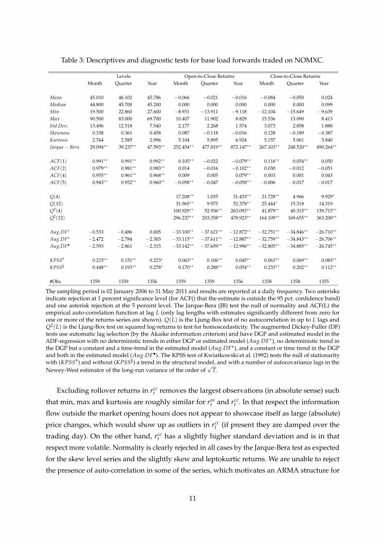
Table 3: Descriptives and diagnostic tests for base load forwards traded on NOMXC.
Levels Open-to-Close Returns Close-to-Close ReturnsMonth Quarter Year Month Quarter Year Month Quarter Year
The sampling period is 02 January 2006 to 31 May 2011 and results are reported at a daily frequency. Two asterisksindicate rejection at 1 percent significance level (for ACF() that the estimate is outside the 95 pct. confidence band)and one asterisk rejection at the 5 percent level. The Jarque-Bera (JB) test the null of normality and ACF(L) theempirical auto-correlation function at lag L (only lag lengths with estimates significantly different from zero forone or more of the returns series are shown). Q(L) is the Ljung-Box test of no autocorrelation in up to L lags andQ2(L) is the Ljung-Box test on squared log-returns to test for homoscedasticity. The augmented Dickey-Fuller (DF)tests use automatic lag selection (by the Akaike information criterion) and have DGP and estimated model in theADF-regression with no deterministic trends in either DGP or estimated model (Aug.DF∗), no deterministic trend inthe DGP but a constant and a time-trend in the estimated model (Aug.DF?), and a constant or time trend in the DGPand both in the estimated model (Aug.DF•). The KPSS test of Kwiatkowski et al. (1992) tests the null of stationaritywith (KPSS†) and without (KPSS‡) a trend in the structural model, and with a number of autocovariance lags in theNewey-West estimator of the long-run variance of the order of
√T.
Excluding rollover returns in rcct removes the largest observations (in absolute sense) such
that min, max and kurtosis are roughly similar for roct and rcc
t . In that respect the information
flow outside the market opening hours does not appear to showcase itself as large (absolute)
price changes, which would show up as outliers in rcct (if present they are damped over the
trading day). On the other hand, rcct has a slightly higher standard deviation and is in that
respect more volatile. Normality is clearly rejected in all cases by the Jarque-Bera test as expected
for the skew level series and the slightly skew and leptokurtic returns. We are unable to reject
the presence of auto-correlation in some of the series, which motivates an ARMA structure for
11
the conditional mean. For example, the monthly rcct has first-order empirical autocorrelation
significantly different from zero. Naturally, the small empirical autocorrelations, in most cases
insignificant from zero, render the returns unpredictable. For the squared series the null of no
autocorrelation is readily rejected in all roct and rcc
t series, which point towards the presence
of (G)ARCH effects and the possibility for volatility prediction. For the price levels we are
unable to reject the presence of a unit root for all specification of the DGP and the model in the
ADF-regression using augmented Dickey-Fuller tests with automatic lag length selection. The
presence of a unit root is readily rejected for all return series. The KPSS test rejects stationarity
in levels and returns. This causes a concern for fractional integration, which due to similar
test results was investigated in more detail in Haugom et al. (2011a). Summarizing, they were
unable to find evidence for a d parameter significantly different from zero when fitting an
ordinary ARFIMA(p, d, q) to the returns. Similarly, the autocorrelogram does appear to exhibit a
hyperbolic decay. Hence, we proceed as if the return series are stationary.
4 Econometric Methodology
We propose to model returns and realized measures of volatility jointly within the Realized
GARCH model framework of Hansen, Huang and Shek (2011). The key variable of interest is
the conditional variance ht = Var [rt |Ft−1 ]. In the Realized GARCH framework ht depends on
its own (truncated) past as usual, but where the traditional framework includes lagged squared
returns, the Realized GARCH framework incorporates a realized measure of volatility (or a
vector of these), xt.9 As such, the model defines a class of GARCH-X models, as in Engle (2002)
and Barndorff-Nielsen and Shephard (2007), where xt is exogenous.10 However, an additional
equation that ties the realized volatility measure to the latent volatility completes the model
and the dynamic properties of both returns and the realized measure are specified. We use a
variant of the Realized GARCH model discussed in Hansen et al. (2010), which is denoted the
Realized EGARCH as it shares certain features with the EGARCH model of Nelson (1991). As
outlined below, the Realized GARCH framework can be compared to nested and more standard
GARCH models, which provides an elegant way to certify possible benefits from utilizing high-
frequency data in a particular market. In applications Hansen, Huang and Shek (2011) showed
with DJIA stocks that the Realized GARCH class led to substantial improvements in in-sample
and out-of-sample empirical fit. Similarly, the chosen subclass here can verify the potential in
the unexplored transaction data considered in this paper. We stress this as the primary interest
of the paper and a horserace between competing models is left for future research.
9Hansen, Huang and Shek (2011) finds that the ARCH-term is insignificant in the Realized GARCH model andwe omit it in the model formulation and in the empirical analysis.
10See also Hansen, Huang and Shek (2011, Section 3) for a comparison to the Multiplicative Error Model (MEM)by Engle and Gallo (2006) and the HEAVY model by Shephard and Sheppard (2010).
12
4.1 The Realized EGARCH Model
The Realized EGARCH model for returns and realized measures of volatility is given by the
mean equation, the GARCH equation and the measurement equation, respectively
rt = µ +s
∑i=1
φi · rt−i + η′Et +√
htzt,
log ht = ω +p
∑j=1
β j · log ht−j +q
∑k=1
γ′k · log xt−k + τ (zt−1) ,
log xt = ξ +ϕ log ht + δ (zt) + ut,
(1)
where
zt ∼ nid (0, 1) and ut ∼ nid (0, Ωu) ,
with m being the number of measurement equations, i.e. we allow for multiple measurement
equations, and zt and ut are mutually independent. We write vectors in bold and matrices
in capital bold. The autocorrelation documented in Table 3 for some of the series motivates
the inclusion of autoregressive terms in the mean equation, and various rollover dummies
and possibly other exogenous terms can be included in Et. We assume market efficiency, i.e.
that such terms are already incorporated in the price, and a refinement of the mean equation
is left for future research. In the GARCH eq. we experiment with the number of lags and
the number of measurement equations. The so-called Samuelson effect is often claimed to be
present in energy markets (see e.g. Benth et al. (2008)), which made us include different time
dependencies in the GARCH eq. However, none of these was found significant and the absence
of the Samuelson effect is further stressed in Table 2, where the realized measures of volatility
do not show signs of time-dependence. Regarding measurement equations, the inclusion of
multiple realized measures is a neat way to show the superiority of some measures over others.
The functions τ (z) and δ (z) are called leverage functions because they model aspects related to
the leverage effect, which refer to the dependence between returns and volatility (see remark
below). Hansen, Huang and Shek (2011) found that a simple second-order polynomial form
provides a good empirical fit and that log z2t was inferior to z2
t . We will adopt this structure and
set τ (z) = τ1z + τ2(z2 − 1
)and δi (z) = δi
1z + δi2(z2 − 1
), i = 1, . . . , m. Hence, E [τ (zt)] = 0
and E[δi (zt)
]= 0, i = 1, . . . , m, for any distribution of zt so long as E [zt] = 0 and Var [zt] = 1.
The normality of ut is motivated by the findings in Andersen, Bollerslev, Diebold and
Labys (2001), Andersen, Bollerslev, Diebold and Ebens (2001), and Andersen et al. (2003), that
document that realized volatility is approximately log-normal. The normality of zt is motivated
by the findings in Andersen, Bollerslev, Diebold and Ebens (2001), that documents that returns
standardized by realized volatility are close to normally distributed. We standardize returns
13
by the conditional variance, which incorporates the realized measure. However, due to results
in Lunde and Olesen (2012) that questions the normality assumption, we compare regular
and bootstrapped forecasts in Section 6. That is, the normality assumption is not crucial to the
estimation, but important for forecasting.
The “intercept” ξ and “slope” ϕ add flexibility to the measurement equation, which may
be required when we link realized measures of volatility that span a shorter period than the
return. As long as xt and ht are roughly proportional we should expect ϕ ≈ 1 and ξ < 0. By
the presence of zt in the measurement equation, it provides a simple way to model the joint
dependence between rt and xt. Tying the realized measure to the conditional variance is nicely
motivated by the fact that the return equation implies that log r2t = log ht + log z2
t , and because
xt is similar to r2t in many ways, albeit a more accurate measure of ht, one may expect that
log xt ≈ log ht + f (zt) + errort. This motivates a logarithmic measurement equation, which
further makes a logarithmic GARCH eq. convenient. A logarithmic specification automatically
ensures a positive variance and as log r2t−1 does not appear in the GARCH eq. (it is replaced by
log xt−1) zero returns do not cause havoc for the specification.
Notice that (1) gives a GARCH eq. similar to an EGARCH-type model motivating the
benchmark
rt = µ +s
∑i=1
φi · rt−i + η′Et +√
htzt,
log ht = ω +p
∑j=1
β j · log ht−j + τ (zt−1) .(2)
As outlined below the log-likelihood function of (1) can be expressed in a way such that it
can be directly compared to the log-likelihood function of (2). Hence, we can easily detect
whether realized measures of volatility lead to improved empirical fit. In-sample in terms of
the log-likelihoods in optimum (Section 5), and out-of-sample in terms forecasting performance
(Section 6).
Remark. The term leverage effect is used to describe the asymmetry in volatility following big
price increases and decreases, respectively. In the classic Black 76’ leverage story an increase
in financial leverage level leads to an increase in equity volatility level with business risk
held fixed. A financial leverage increase can come from stock price decline while the debt
level is fixed. In energy markets there is evidence of a so-called inverse leverage effect. The
volatility tends to increase with the level of prices, since there is a negative relationship
between inventory and prices (see for instance Deaton and Laroque (1992)). Little available
inventory means higher and more volatile prices. The application will show whether or
not this effect carries over to the forward market.
14
4.2 Estimation
The log-likelihood function is given by
` (r, x; θ) = −T (m + 1)2
· log 2π − 12
T
∑t=1
(log ht + z2
t + log |Ωu|+ u′tΩ−1u ut
),
where |A| is the determinant of the matrix A and θ is the parameter vector
The value of Ωu that maximizes the likelihood among the class of all symmetric positive definite
matrices is (see e.g. Hamilton (1994))
Ωu =1T
T
∑t=1
utu′t,
such that by the rules of the inverse we can express the log-likelihood function as (constant
omitted)
−2` (r, x; θ) =T
∑t=1
[log ht + z2
t]
︸ ︷︷ ︸=−2`(r)
+ T(log∣∣Ωu
∣∣+ 1)︸ ︷︷ ︸
=−2`(x|r )
. (3)
This reduces the parameter set that the optimizer has to search over. If one is only interested
in one-step ahead modeling, specifying the measurement equation becomes redundant and
the parameters in the model are further reduced. Standard GARCH models do not model
xt, so the log-likelihood we obtain for these models (here the EGARCH model) cannot be
compared to those of the Realized GARCH model. However, the expression for the log-likelihood
above proves useful in this respect as the first term is a partial log-likelihood, which is directly
comparable to the log-likelihood of standard models.
5 Estimation Results
In this section we present empirical results for the Realized GARCH model with a range
of specifications. We limit the exposition to the quarterly contract, which is the most liquid
of the three.11 We focus on close-to-close returns and use open-to-close returns only for one
specification of the Realized GARCH and its benchmark to highlight characteristics of the
parameters in the measurement equation. We utilize primarily the realized kernel as the realized
measure of volatility (columns 2− 9), but present results for five realized variances for one
11A web appendix with results for the nearby month and nearby year contracts is available upon request.
15
model specification for comparison.12 We use EG to denote the conventional EGARCH in Eq. 2
and REG to denote the Realized EGARCH in Eq. 1 with the choice of p and q in parenthesis.
Focusing on parameter estimates, the realized measure loadings are large and the typical
GARCH effects are of a smaller magnitude compared to conventional GARCH models. However,
the lagged conditional volatility is still the dominant term. These findings are in line with results
for individual stocks in Hansen et al. (2010). The estimates of the parameters in the leverage
function δ are similar to the ones reported in Hansen, Huang and Shek (2011) and Hansen et al.
(2010) and describe an asymmetric volatility response to positive vs. negative shocks. However,
the τ1 estimate is in most cases found to be insignificant from zero, where Hansen, Huang and
Shek (2011) and Hansen et al. (2010) found negative parameter estimates. This is in line with the
comments above on the interpretation of leverage effects in energy markets. The presence of a
leverage effect in NOMXC forwards is questionable and omitting τ leads only to a negligible
drop in the log-likelihood function. Omitting δ leads on the other hand to a rather large drop in
the log-likelihood. The roll-over effect was included in different ways and results are reported
for the simplest one; one dummy in the mean equation. The estimate is hardly significantly
different from zero and other parameter estimates are similar to those of the other specifications.
The realized measures are based on data spanning the trading session only, and as expected ξ is
negative and ϕ close to one in all cases. Notice also, that the estimates are smaller (in absolute
sense) as expected for the open-to-close series.
Comparing models, REG(1, 1)? has the best empirical fit in-sample measured by the log-
likelihood, ` (r, x), and the realized kernel appear inferior. However, for the partial log-likelihood
the results are more unclear, and the performance of models based on the realized kernel appear
similar to that of models utilizing realized variances.13 The partial log-likelihood is directly
comparable to the log-likelihood of traditional EGARCH-models, and the improvements are
unquestionable for all series.14 That is, utilizing transactions data improves the empirical fit
of the model. To visualize the time-dependent level and pattern of the conditional volatility,
which stress the importance of active risk and portfolio management, we present in Figure 3 the
resulting conditional variances of time for the underlined model specification in Table 4.
12RV(1 tick), RV(1800 sec), RV(1800 sec)∗, RV(300 sec) RV(300 sec)∗ in columns 10− 14, respectively.13One should compare column 4 to columns 10− 14.14One should compare column 1 to 2, and column 3 to 4.
16
Tabl
e4:
Res
ults
for
the
Rea
lized
EGA
RC
Hm
odel
for
the
quar
terl
yfir
stne
arby
for
base
load
forw
ards
trad
edon
NO
MX
C.
Ope
n-to
-Clo
seR
etur
nsC
lose
-to-
Clo
seR
etur
ns
Mod
elEG
(1,1
)R
EG(1
,1)
EG(1
,1)
REG
(1,1
)R
EG(1
,1)
REG
(1,1
)R
EG(1
,1)
REG
(2,2
)R
EG(1
,1)ro
llR
EG(1
,1)∗
REG
(1,1
)?R
EG(1
,1)•
REG
(1,1
)†R
EG(1
,1)‡
Pane
lA:P
oint
Esti
mat
esan
dLo
g-Li
kelih
ood
log
h01.
823
(0.6
65)
−0.
167
(1.2
74)
0.30
4(1
.034)
1.13
9(0
.675)
1.14
0(0
.676)
0.80
0(0
.702)
0.07
0(0
.810)
3.37
1(4
.628);2
.450
(1.4
45)
0.85
0(0
.965)
1.36
0(0
.764)
0.85
9(0
.737)
0.86
5(0
.759)
1.17
3(0
.735)
1.15
9(0
.723)
µ−
0.00
3(0
.052)
0.03
5(0
.049)
0.07
4(0
.089)
0.08
7(0
.081)
0.08
8(0
.082)
0.09
0(0
.081)
0.08
5(0
.080)
0.08
4(0
.081)
−0.
059
(0.0
81)
0.10
1(0
.081)
0.09
4(0
.079)
0.08
6(0
.080)
0.09
5(0
.081)
0.09
7(0
.082)
φr;
...;
φ1
0.04
7(0
.027)
−0.
018
(0.0
27)
;0.0
51(0
.028)
η1.
065
(0.6
60)
ω0.
059
(0.0
16)
0.23
9(0
.032)
0.26
2(0
.059)
0.77
9(0
.063)
0.77
4(0
.063)
0.76
8(0
.062)
0.75
6(0
.062)
0.21
5(0
.023)
0.87
6(0
.073)
0.88
0(0
.067)
0.54
3(0
.053)
0.73
2(0
.066)
0.78
6(0
.066)
0.75
0(0
.066)
βp;
...;
β1
0.95
9(0
.010)
0.63
5(0
.030)
0.89
2(0
.024)
0.53
8(0
.030)
0.54
2(0
.029)
0.54
1(0
.030)
0.53
9(0
.031)
−0.
284
(0.0
00)
;1.1
55(0
.009)
0.45
6(0
.036)
0.48
3(0
.032)
0.64
3(0
.028)
0.54
6(0
.033)
0.50
5(0
.033)
0.48
9(0
.032)
γq;
...;
γ1
0.31
4(0
.029)
0.32
3(0
.029)
0.31
8(0
.028)
0.32
6(0
.030)
0.34
1(0
.030)
−0.
246
(0.0
30)
;0.3
38(0
.030)
0.43
2(0
.032)
0.41
1(0
.037)
0.29
1(0
.027)
0.33
8(0
.031)
0.36
3(0
.033)
0.36
3(0
.033)
τ 1−
0.01
0(0
.020)
0.00
1(0
.011)
−0.
047
(0.0
25)
0.00
6(0
.010)
0.00
2(0
.010)
0.00
7(0
.011)
0.00
1(0
.005)
0.01
0(0
.012)
−0.
003
(0.0
10)
0.00
4(0
.012)
0.00
9(0
.011)
0.00
5(0
.010)
0.00
6(0
.010)
τ 20.
109
(0.0
13)
0.06
7(0
.009)
0.03
6(0
.009)
−0.
002
(0.0
02)
−0.
002
(0.0
02)
−0.
002
(0.0
02)
0.00
1(0
.001)
−0.
004
(0.0
03)
0.00
0(0
.002)
−0.
000
(0.0
03)
−0.
002
(0.0
03)
−0.
001
(0.0
02)
−0.
001
(0.0
02)
α ξ−
0.49
6(0
.070)
−1.
992
(0.2
36)
−2.
010
(0.2
38)
−1.
949
(0.2
31)
−1.
807
(0.2
06)
−2.
005
(0.1
77)
−1.
537
(0.1
48)
−1.
772
(0.2
00)
−1.
458
(0.1
82)
−1.
738
(0.2
09)
−1.
768
(0.2
16)
−1.
662
(0.2
32)
ϕ0.
980
(0.0
43)
1.25
0(0
.099)
1.25
8(0
.100)
1.23
3(0
.097)
1.17
6(0
.087)
1.25
8(0
.076)
1.05
1(0
.062)
1.10
0(0
.084)
1.05
1(0
.077)
1.15
8(0
.088)
1.19
1(0
.091)
1.23
5(0
.097)
δ 1−
0.02
8(0
.015)
−0.
062
(0.0
16)
−0.
061
(0.0
16)
−0.
061
(0.0
16)
−0.
060
(0.0
16)
−0.
057
(0.0
16)
−0.
056
(0.0
14)
−0.
064
(0.0
19)
−0.
068
(0.0
17)
−0.
063
(0.0
15)
−0.
061
(0.0
15)
δ 20.
158
(0.0
10)
0.01
4(0
.004)
0.01
4(0
.004)
0.01
3(0
.004)
0.01
3(0
.004)
0.01
2(0
.004)
0.01
3(0
.003)
0.02
4(0
.005)
0.01
7(0
.004)
0.01
6(0
.004)
0.01
4(0
.003)
`(r,
x)−
1301
.355
−21
07.7
31−
2108
.173−
2119
.071−
2107
.588
−20
99.8
86−
2107
.320
−18
81.7
34−
2329
.336−
2191
.845−
2038
.432−
2005
.894
Pane
lB:A
uxili
ary
Stat
isti
cs
`(r)
−16
76.9
43−
1656
.042−
2319
.685−
2254
.163−
2254
.153−
2254
.052−
2251
.036
−22
48.9
27−
2252
.652
−22
52.9
24−
2239
.148−
2245
.208−
2253
.369−
2256
.259
σ2 u
0.21
80.
296
0.29
70.
301
0.29
80.
295
0.29
70.
213
0.42
00.
340
0.26
80.
254
The
sam
plin
gpe
riod
is02
Janu
ary
2006
to31
May
2011
.EG
deno
tes
the
conv
entio
nalE
GA
RC
Hin
Eq.2
and
REG
deno
tes
the
Rea
lized
EGA
RC
Hin
Eq.1
with
the
choi
ceof
pan
dq
inp
aren
thes
is.P
anel
Aco
ntai
nsp
aram
eter
esti
mat
esan
dfo
rth
eR
EG
-mod
els
also
the
full
log-
likel
ihoo
d.P
anel
Bco
ntai
nsau
xilia
ryst
atis
tics
;`(r)
isth
ere
stri
cted
log-
likel
ihoo
d,a
ndσ
2 uis
the
esti
mat
edse
cond
mom
ento
fuas
outl
ined
in4.
2.C
olum
nson
ean
dtw
ous
esop
en-t
o-cl
ose
retu
rns
and
the
rem
aini
ngco
lum
nsus
escl
ose-
to-c
lose
retu
rns.
The
real
ized
kern
elis
used
asou
rre
aliz
edm
easu
reof
vola
tilit
yin
colu
mns
2−
9an
dR
EG
(1,1
)∗us
esRV
(0ti
ck) ,
RE
G(1
,1)?
uses
RV(1
800
sec)
,R
EG(1
,1)•
uses
RV(1
800
sec)∗ ,
REG
(1,1
)†us
esRV
(300
sec)
,and
REG
(1,1
)‡us
esRV
(300
sec)∗ .
The
unde
rlin
edm
odel
spec
ifica
tion
isus
edin
follo
win
gse
ctio
ns.S
tand
ard
erro
rsin
pare
nthe
sis
belo
wth
ees
tim
ates
.
17
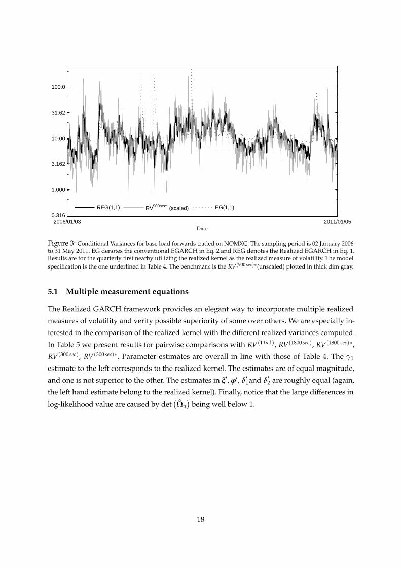
2006/01/03 2011/01/050.316
1.000
3.162
10.00
31.62
100.0
Date
REG(1,1) RV900sec* (scaled) EG(1,1)
Figure 3: Conditional Variances for base load forwards traded on NOMXC. The sampling period is 02 January 2006to 31 May 2011. EG denotes the conventional EGARCH in Eq. 2 and REG denotes the Realized EGARCH in Eq. 1.Results are for the quarterly first nearby utilizing the realized kernel as the realized measure of volatility. The modelspecification is the one underlined in Table 4. The benchmark is the RV(900 sec)∗(unscaled) plotted in thick dim gray.
5.1 Multiple measurement equations
The Realized GARCH framework provides an elegant way to incorporate multiple realized
measures of volatility and verify possible superiority of some over others. We are especially in-
terested in the comparison of the realized kernel with the different realized variances computed.
In Table 5 we present results for pairwise comparisons with RV(1 tick), RV(1800 sec), RV(1800 sec)∗,
RV(300 sec), RV(300 sec)∗. Parameter estimates are overall in line with those of Table 4. The γ1
estimate to the left corresponds to the realized kernel. The estimates are of equal magnitude,
and one is not superior to the other. The estimates in ξ′, ϕ′, δ′1and δ′2 are roughly equal (again,
the left hand estimate belong to the realized kernel). Finally, notice that the large differences in
log-likelihood value are caused by det(Ωu)
being well below 1.
18
Table 5: Results for the Realized EGARCH model with multiple measurement equations.
Model REG(1,1) REG(1,1)? REG(1,1)• REG(1,1)† REG(1,1)‡
The sampling period is 02 January 2006 to 31 May 2011. Results are for the underlined model specification in Table 4.REG denotes the Realized EGARCH in Eq. 1 with the choice of p and q in parenthesis. REG(1,1) uses RK and RV(0 tick)
as the realized measures of volatility, REG(1,1)? uses RK and RV(1800 sec), REG(1,1)• uses RK and RV(1800 sec)∗,REG(1,1)† uses RK and RV(300 sec), and REG(1,1)‡ uses RK and RV(300 sec)∗. Standard errors in parenthesis below theestimates.
5.2 Diagnostics
We present now a limited number of diagnostics for the underlined REG(1, 1) model specification
in Table 4 utilizing the realized kernel. To check the model assumption of normality we present
quantile-quantile plots in Figure 4, which compare the empirical distribution of the standardized
residuals, zt and ut, to a normal distribution. The normality of zt is clearly rejected with excess
kurtosis far beyond 0. The results suggest that for forecasting one may consider a bootstrap
approach (see Section 6).
19
−4 −2 0 2 4−10
−5
0
5
10
15
Quantiles of Standard Normal Distribution
Quan
tilesof
Empirical
Distribution
ofz
Jarque-Bera test probability for normal distribution: 0.001
−4 −2 0 2 4−3
−2
−1
0
1
2
3
Quantiles of Standard Normal Distribution
Quan
tilesof
Empirical
Distribution
ofu
Jarque-Bera test probability for normal distribution: 0.001
Figure 4: Residual QQ-plots for the REG(1, 1) fitted to base load forwards traded on NOMXC. The sampling periodis 02 January 2006 to 31 May 2011. Results are for the standardized residuals from the REG(1, 1) for quarterly firstnearby utilizing the realized kernel as the realized measure of volatility, and using the underlined model specificationin Table 4.
Table 6 presents results on autocorrelation and heteroscedasticity in the standardized residu-
als. We do not detect signs of heteroscedasticity, and hence, the model is successful in this sense.
With respect to autocorrelation, the results point towards the inclusion of a autoregressive term
in the mean equation.
Table 6: Residual diagnostics for the REG(1, 1) fitted to base load forwards traded on NOMXC.
The sampling period is 02 January 2006 to 31 May 2011. Results are for the standardized residuals from the REG(1, 1)for the quarterly first nearby utilizing the realized kernel as the realized measure of volatility, and using theunderlined model specification in Table 4. ACF(L) is the empirical autocorrelation function at lag L and Q(L) is theLjung-Box test of no autocorrelation in up to L lags. Two asterisks indicate rejection at 1 percent significance level(for ACF() that the estimate is outside the 95 pct. confidence band) and one asterisk rejection at the 5 percent level.
20
6 Forecasting
We now discuss how multi-step predictions of volatilities as well as return density forecasts can
be obtained from the Realized EGARCH(1,1) model in the case of one measurement equation.
Generalizations are straightforward. Let ht+1 := log ht+1. Point forecasts turn out to be easy
to obtain owing to the fact that the vector ht+1 can be represented as an ARMA(1,1) system.
Substituting the measurement equation into the equation for the corresponding conditional
moment one obtains
ht+1 = C + Aht + Bεt,
where εt = (δ(zt), τ(zt), ut)ᵀ, and C, A and B are given by
C = ω + γξ, A = β + γϕ, B =[
γ 1 γ]
,
which follow from the estimation up until time t. The innovation process, εt, is a martingale
difference sequence and it follows that
E(ht+k|ht) = Ak ht +
k−1
∑j=0
AjC,
which can be used to produce a k-step ahead forecast of ht+k. We note that non-linearity implies
E[exp(ht)
]6= exp E
[ht]. Forecast of the conditional distribution of ht+k|Ft, which can be used to
deduce unbiased forecasts of the non-transformed variables, e.g., ht = exp(ht), can be obtained
by simulation methods or the bootstrap. In the simulation approach, we first generate
ζt =
(zt
ut
)∼ N
(0,
[1 0
0 σ2u
]), t = 1, . . . n,
and thus εt can be computed. Based on S simulations we estimate ht+k as 1S ∑S
s=1 exp(ht+k).
Alternatively, a bootstrap approach can be preferable if the Gaussian assumption concerning the
distribution of ζt is questionable. From the estimated model we obtain residuals, (ζ1, . . . , ζn),
from which we draw re-samples instead of sampling from the Gaussian distribution. Time series
for ht can now be generated from the bootstrapped residuals ζ∗t in the same manner as with
simulated ζt.Below we present point forecasts and results for 1-step-ahead predictions, and 5-step and 20-
step ahead predictions with bootstrapped innovations.15 We set S = 1000 and use the REG(1, 1)
with no deterministic components and with the realized kernel as the realized measure of
15Results based on simulated innovations can be found in the web appendix. However, differences to the onespresented here are not visible.
21
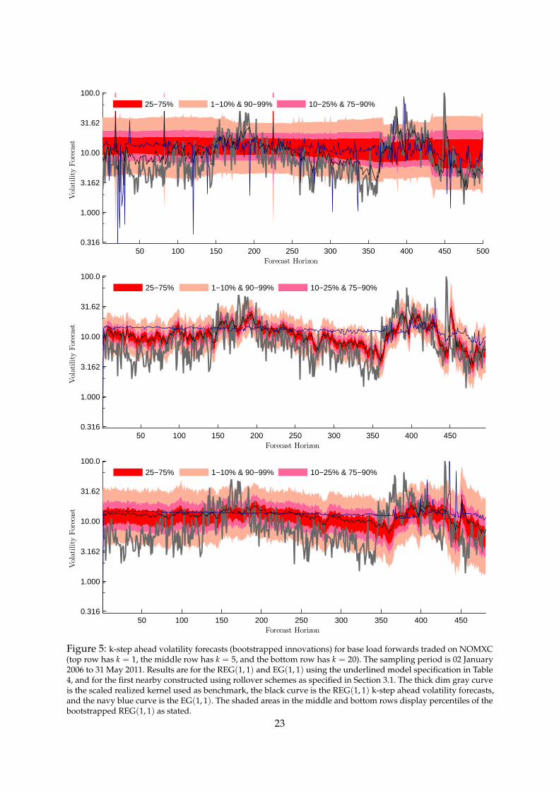
volatility. The horizon is set to 500 leaving 858 observations for each estimation in a rolling-
window setup. Figure 5 displays the resulting series. The thick dim gray line is the 15 minute
realized variance subsampled every minute, RV(900 sec)?, scaled by a factor of 3.2 (= 24/7.5)
used as benchmark, the black line is forecasts from the REG(1, 1) and the blue line is forecasts
from the EG(1, 1). For the 1-step ahead predictions shaded areas correspond to percentiles from
the unconditional distribution of h, and for the 5-step and 20-step ahead predictions shaded
areas are percentiles from the S simulations.
Looking at the 1-step-ahead predictions in the top row of Figure 5, improvements are not
easily seen by the naked eye. However, we will argue that for the quarterly series in particular,
REG(1, 1) has better capabilities to follow the pattern in the RV(900 sec)? benchmark. Results
are sligtly clearer in the middle and bottom row in Figure5, where the REG(1, 1) appear more
responsive than the EG(1, 1), which is inadequately smooth. To more formally compare the
forecast performance of the models we apply the model confidence set (MCS) of Hansen,
Lunde and Nason (2011) in Table 7. Results for the monthly and yearly contracts are included.
Briefly, the objective of the MCS procedure is to determine the set of “best” models,M?, from a
collection of modelsM0, where “best” here is defined by a loss function. Thus, one can view
the MCS as a set of models that includes the “best” models with a given level of confidence.
With informative data the MCS will consist only of the best model, and less informative data
may result in a MCS with several models. We refer to Hansen, Lunde and Nason (2011) for
details. In Table 7M0 consists of two models in the case of 1-step ahead predictions, and four
models for 5- and 20-step ahead predictions. We take as loss function the mean squared error
(MSE), where the “true value” is taken to be RV(900 sec)?. In Table 7 one asterisk indicates that the
model belongs to M?90%. For 1-step ahead predictions is REG(1, 1) consistently in M?
90% with
pMCS ' 1. Only for the monthly series is EG(1, 1) in M?90%. For 5- and 20-step ahead predictions
for the quarterly and yearly series is the REG(1, 1) with bootstrapped innovations consistently in
M?90%, which is never the case for EG(1, 1). For the monthly series is the EG(1, 1) with simulated
innovations consistently in M?90%. This is in line with expectations, as we would expect the
Realized EGARCH to perform better as compared to a conventional EGARCH when liquidity is
improved.
22
50 100 150 200 250 300 350 400 450 5000.316
1.000
3.162
10.00
31.62
100.0
Forecast Horizon
VolatilityForecast
25−75% 1−10% & 90−99% 10−25% & 75−90%
50 100 150 200 250 300 350 400 4500.316
1.000
3.162
10.00
31.62
100.0
Forecast Horizon
VolatilityForecast
25−75% 1−10% & 90−99% 10−25% & 75−90%
50 100 150 200 250 300 350 400 4500.316
1.000
3.162
10.00
31.62
100.0
Forecast Horizon
VolatilityForecast
25−75% 1−10% & 90−99% 10−25% & 75−90%
Figure 5: k-step ahead volatility forecasts (bootstrapped innovations) for base load forwards traded on NOMXC(top row has k = 1, the middle row has k = 5, and the bottom row has k = 20). The sampling period is 02 January2006 to 31 May 2011. Results are for the REG(1, 1) and EG(1, 1) using the underlined model specification in Table4, and for the first nearby constructed using rollover schemes as specified in Section 3.1. The thick dim gray curveis the scaled realized kernel used as benchmark, the black curve is the REG(1, 1) k-step ahead volatility forecasts,and the navy blue curve is the EG(1, 1). The shaded areas in the middle and bottom rows display percentiles of thebootstrapped REG(1, 1) as stated.
23
Table 7: MCS Results for base load forwards traded on NOMXC.
MSEs and MCS p-values for the different forecasts. The forecasts in M∗90% are identified by an asterisk. Results arefor the underlined model specification in Table 4. EG denotes the conventional EGARCH in Eq. 2 and REG denotesthe Realized EGARCH in Eq. 1.
7 Conclusion
In this paper we have explored the transaction records from NOMXC back to January 2006
and discussed the issue of construction of continual nearby contracts. We have estimated a
range of realized measures of volatility, and investigated similarities and differences of such.
The realized volatility measures are used to enrich the information set of GARCH models in
the Realized GARCH framework of Hansen, Huang and Shek (2011) and Hansen et al. (2010).
Estimations clearly reveal a gain from utilizing data at higher frequencies. Compared to ordinary
EGARCH models, which is nested in the Realized EGARCH considered, improved empirical fit
is obtained, in-sample as well as out-of-sample. The out-of-sample assessment is based on 1-, 5-
and 20-step-ahead regular and bootstrapped rolling-window forecasts. The Realized EGARCH
outperforms its nested benchmark visually and in terms of the MCS of Hansen, Lunde and
Nason (2011). Throughout, the obtained results illustrate the importance of careful volatility
estimation as the level is time-dependent but predictable. An appealing extension is in the
multivariate setting, where covolatilities between the different NOMXC forwards, and between
the forwards and other energy markets as coal, gas, and oil, are important to many (e.g. energy
and utility companies).
24
References
Andersen, T. G., Bollerslev, T. and Diebold, F. X. (2009), Parametric and nonparametric volatility
measurement, in L. P. Hansen and Y. Ait-Sahalia, eds, ‘Handbook of Financial Econometrics’,
North-Holland, Amsterdam.
Andersen, T. G., Bollerslev, T., Diebold, F. X. and Ebens, H. (2001), ‘The distribution of realized
stock return volatility’, Journal of Financial Economics 61(1), 43–76.
Andersen, T. G., Bollerslev, T., Diebold, F. X. and Labys, P. (2001), ‘The distribution of exchange
rate volatility’, Journal of the American Statistical Association 96(453), 42–55. Correction published
in 2003, volume 98, page 501.
Andersen, T. G., Bollerslev, T., Diebold, F. X. and Labys, P. (2003), ‘Modeling and forecasting