Modeling and optimization of HVAC systems using artificial neural network and genetic algorithm
Nabil Nassif ()
North Carolina A&T State University, Department of CAAE Engineering, 455 McNair Hall, 1601 E. Market Street, Greensboro, NC 27411, USA Abstract Intelligent energy management and control system (EMCS) in buildings offers an excellent means of reducing energy consumptions in HVAC systems while maintaining or improving indoor environmental conditions. This can be achieved through the use of computational intelligence and optimization. The paper thus proposes and evaluates a model-based optimization process for HVAC systems using evolutionary algorithm for optimization and artificial neural networks for modeling. The process can be integrated into the EMCS to perform several intelligent functions and achieve optimal whole-system performance. The proposed models and the optimization process are tested using data collected from an existing HVAC system. The testing results show that the models can capture very well the system performance, and the optimization process can reduce cooling energy consumption by about 11% when compared to the traditional operating strategies applied.
Keywords HVAC systems,
self tuning models,
artificial neural network,
energy management and control
systems,
optimization Article History Received: 23 August 2012
Great efforts have been invested in minimizing the energy costs associated with the operation of HVAC systems. Intelligent Energy Management and Control Systems (EMCS) can provide an effective way of decreasing energy costs in HVAC systems while maintaining indoor environmental conditions (ASHRAE 2011). This EMCS can include several intelligent functions such as optimum set points and operating modes (ASHRAE 2011; Nassif 2012; Nassif et al. 2005; Wang and Jin 2000; Zheng and Zaheer-Uddin 1996) and fault detection and diagnosis (Seem 2007; Lee et al. 1996). The intelligent EMCS can be achieved through the use of the computational intelligence and optimization (Hagras 2008; Kusiak and Xu 2012). The paper thus proposes model- based optimization process for HVAC systems using genetic algorithm and artificial neural networks. The process can be integrated into the EMCS to perform such intelligent functions and achieve optimal whole-system performance. The HVAC optimization problems are solved using the
genetic algorithm (GA) inspired by natural evolution which is successfully applied to a wide range of applications including HVAC systems (Deb 2001; Goldberg 1989; Xu et al. 2009; Mossolly et al. 2009). The HVAC optimization problems are dynamic and the problem changes over the course of the optimization. Thus, the GA with proper enhancement and the ability of continuously track the movement of the optimum over time are developed and used. Components models are required for the optimization process and for any other functions. Depending on the type of functions and the accuracy required, the models can vary from simple to more sophisticated calculations. However, it is of practical importance to develop a simple, yet accurate and reliable model to better match the real behavior of the subsystems and overall system over the entire operating range. Models can be developed by two distinct methods (ASHRAE 2009): forward models and data-driven models. Forward models may need detailed physical information that is not always available. Moreover, it is almost impossible to develop a model based on physical knowledge that perfectly
BUILD SIMUL (2014) 7: 237–245 DOI 10.1007/s12273-013-0138-3
Nassif / Building Simulation / Vol. 7, No. 3
238
simulates the real system behavior. In addition, the characteristics of the real system can change over time; the physical model with fixed parameters may no longer be able to track correctly the real performance. Alternatively, data-driven models are another approach to be used for existing systems. In this paper, we will explore the use of artificial neural network as data-driven and self tuning models in HVAC applications, focusing on optimization and control. The proposed models are tested evaluated using data collected over three summer months from a typical existing HVAC system. However, the optimization process was evaluated by simulations applied to the same system.
2 HVAC and EMC system configuration
Figure 1 shows a schematic diagram of a typical HVAC system and the optimization process integrated into EMCS. Included in this schematic are the proposed artificial neural network (ANN) models and how they interact within the overall system. A typical HVAC system that uses variable air volume (VAV) control is illustrated in Fig. 1. It consists
mainly of (i) the return and supply fans, (ii) the outdoor, discharge, and recirculation dampers, (iii) the air handling unit (AHU) with components such as filter and cooling and heating coils, (iv) the pressure-independent VAV terminal boxes, and (v) the local-loop controllers (i.e., C1, C2, and C3). The supply air temperature is controlled by the controller (C1). The duct static pressure is controlled by the controller (C2). The zone air temperature at any particular zone n is controlled by the controller (C3 (n)).
The EMCS collects the measured data (real data) from components or subsystems. The ANN models are con-tinuously trained using the real data to better match the real behavior of the subsystems and overall system. The training algorithm used is Levenberg-Marquardt, which is a built-in algorithm in MATLAB. As recommended in this paper for optimal control strategy, at each time interval (e.g. 10 min), the ANN models provide optimal whole system performance through determining optimal set points and operation sequences. A genetic algorithm as described in next section is used to solve the optimization problem.
Fig. 1 Typical HVAC system and EMCS along with the proposed ANN models and optimization process
Nassif / Building Simulation / Vol. 7, No. 3
239
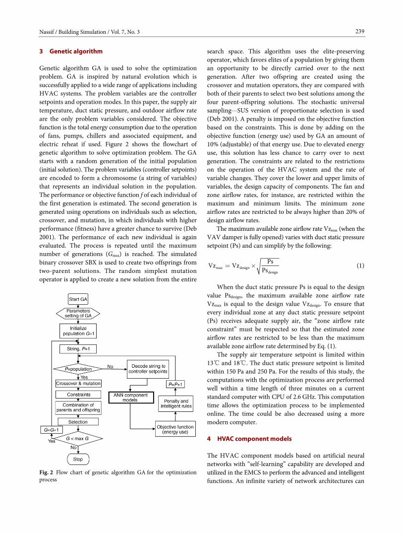
3 Genetic algorithm
Genetic algorithm GA is used to solve the optimization problem. GA is inspired by natural evolution which is successfully applied to a wide range of applications including HVAC systems. The problem variables are the controller setpoints and operation modes. In this paper, the supply air temperature, duct static pressure, and outdoor airflow rate are the only problem variables considered. The objective function is the total energy consumption due to the operation of fans, pumps, chillers and associated equipment, and electric reheat if used. Figure 2 shows the flowchart of genetic algorithm to solve optimization problem. The GA starts with a random generation of the initial population (initial solution). The problem variables (controller setpoints) are encoded to form a chromosome (a string of variables) that represents an individual solution in the population. The performance or objective function f of each individual of the first generation is estimated. The second generation is generated using operations on individuals such as selection, crossover, and mutation, in which individuals with higher performance (fitness) have a greater chance to survive (Deb 2001). The performance of each new individual is again evaluated. The process is repeated until the maximum number of generations (Gmax) is reached. The simulated binary crossover SBX is used to create two offsprings from two-parent solutions. The random simplest mutation operator is applied to create a new solution from the entire
Fig. 2 Flow chart of genetic algorithm GA for the optimization process
search space. This algorithm uses the elite-preserving operator, which favors elites of a population by giving them an opportunity to be directly carried over to the next generation. After two offspring are created using the crossover and mutation operators, they are compared with both of their parents to select two best solutions among the four parent-offspring solutions. The stochastic universal sampling—SUS version of proportionate selection is used (Deb 2001). A penalty is imposed on the objective function based on the constraints. This is done by adding on the objective function (energy use) used by GA an amount of 10% (adjustable) of that energy use. Due to elevated energy use, this solution has less chance to carry over to next generation. The constraints are related to the restrictions on the operation of the HVAC system and the rate of variable changes. They cover the lower and upper limits of variables, the design capacity of components. The fan and zone airflow rates, for instance, are restricted within the maximum and minimum limits. The minimum zone airflow rates are restricted to be always higher than 20% of design airflow rates.
The maximum available zone airflow rate Vzmax (when the VAV damper is fully opened) varies with duct static pressure setpoint (Ps) and can simplify by the following:
max designdesign
PsVz VzPs
= ´ (1)
When the duct static pressure Ps is equal to the design value Psdesign, the maximum available zone airflow rate Vzmax is equal to the design value Vzdesign. To ensure that every individual zone at any duct static pressure setpoint (Ps) receives adequate supply air, the “zone airflow rate constraint” must be respected so that the estimated zone airflow rates are restricted to be less than the maximum available zone airflow rate determined by Eq. (1).
The supply air temperature setpoint is limited within 13℃ and 18℃. The duct static pressure setpoint is limited within 150 Pa and 250 Pa. For the results of this study, the computations with the optimization process are performed well within a time length of three minutes on a current standard computer with CPU of 2.6 GHz. This computation time allows the optimization process to be implemented online. The time could be also decreased using a more modern computer.
4 HVAC component models
The HVAC component models based on artificial neural networks with “self-learning” capability are developed and utilized in the EMCS to perform the advanced and intelligent functions. An infinite variety of network architectures can
Nassif / Building Simulation / Vol. 7, No. 3
240
be used for this purpose, but in the interest of conserving computer time the simplest structure needs to be considered. Each model has only one hidden layer with twenty neurons and with hyperbolic activation function (tanch). The model has the output layer with one neuron and an activation function based on the sum of the weighted hidden layer neurons. Each neuron also has bias.
The models described here are the fan, cooling coil, and chiller models. Those models can be used for various applications but the inputs and the outputs have to be clearly defined. The inputs of the models for a specific application may become outputs in other application. For instance, in the control application, the controlled variables such as duct static pressure and supply air temperature are the outputs of the fan model and cooling coil model, respectively. For the optimization, the model outputs are estimates of the energy consumptions (the objective function) such as fan power and compressor power (see the second and third rows in Table 1). Although the models were validated and tested for both cases, the detailed discussions were only made for the optimization application as our main focus in this paper is to test the proposed optimization process. Such process needs the models as shown in Fig. 3. The inputs of the fan model are the system airflow rate and static pressure (duct static pressure setpoint) and the output is fan power. The inputs of the cooling coil model are fan airflow rate, entering liquid temperature (chilled water supply temperature set- point), entering air dry bulb temperature and humidity ratio, supply air dry bulb temperature (supply air temperature
setpoint), and the output is cooling load. The inputs of the chiller model are the cooling coil load, chilled water supply temperature, and the condenser water temperature, and the output is the compressor power. Additional basic calculations are also required for the optimization, including a zone model. The zone model is to determine the zone airflow rates, local heating energy use, and return air conditions based on thermal loads. The calculations are based on the steady state heat balance equation for each zone in which the sensible load is a function of airflow rate and the differences between the space and supply air temperatures. Similarly, the humidity is determined using the latent load. The loads are determined from the same model but with an inverse form using measured data of the previous period and then the loads are assumed to be constant during the current optimization period. The electric reheat is considered here and it turns on only when the airflow rate reaches its minimum level (e.g., 20% of design airflow rate) and the space temperature becomes lower than heating setpoint. The system airflow rate used as an input for cooling or fan model is equal to the sum of zone airflow rates found from the zone model. An iteration process should be applied to estimate the return air conditions, the initial cooling coil leaving air humidity ratio is assumed, and the new value is calculated and reused. This iterative process continues calculating through the loop several times until the values of cooling coil leaving air humidity ratio stabilize within a specified tolerance. The calculation presented above is similar to that for a VAV model in the HVAC toolkit
Table 1 Model testing results
Results
Models Application Model output Model test Samples MaxE MAE CV(%)
Training 34560 × 3 0.475 0.19 1.13
Validation 6912 × 3 0.487 0.20 1.2 Optimization Power (kW)
Validation 20 0.84 0.42 2.12 Optimization Power (kW)
Testing 18 1.23 0.58 3.18 Chiller model
Control Chilled water temperature (℃) Not tested
Nassif / Building Simulation / Vol. 7, No. 3
241
(Brandemuehl et al. 1993). The minimum airflow rate based on the ASHRAE standard 62.1 2010 (ASHRAE 2010) is included in the optimization calculations. The outdoor air is determined by the multi-zone procedure of ASHRAE 62.1 standard based on the actual zone airflow rates. The advantage of including the minimum outdoor standard procedure in the whole optimization process is to minimize the energy use while respecting the ventilation requirements by the current standard. The standard prescribes two ventilation rates, one intended to dilute the contaminants generated by occupants (Rp) and the other for building-related sources (Ra). The required minimum breathing zone outdoor air rate is as a function of the number of zone occupants Pz and the zone floor area Az. When the economizer is not activated, the minimum outdoor airflow rate Vot is found:
ouot
v
VVE
= (2)
The uncorrected outdoor air intake flow Vou and system ventilation efficiency Ev are given:
ou p z a z( )i i i i
V R P R A= ´ + ´å (3)
p z a zouv
s zmin 1 i i i i
i
R P R AVEV V
´ + ´= + -( ) (4)
The zone airflow rates ziV and system flow rate Vs (fan airflow
rate) in Eq. (4) are optimally found by the optimization process. The term inside the parenthesis is calculated for each zone i and the Ev is equal to the minimum value.
5 Modeling testing
Data from an existing VAV system are collected over three summer months (June, July, and August) at one-minute intervals. The first 23 days data of each month (34560 data points) were randomly divided into two types of samples: 80% for training (27648 data points) and 20% for validation (6912 data points). The last 7 days of each month (10080 data points) are kept for the model testing and to define the model accuracy. During the training, the network is adjusted according to its error using Levenberg-Marquardt optimiza-tion. The validation samples are used to measure network generalization, and to halt training when generalization stops improving. The testing data have no effect on training and provide an independent measure of network performance after training. The model performance is measured by the mean absolute error MAE, maximum error MaxE, and the coefficient of variation CV, which is defined as the ratio of the standard deviation to the mean.
Figure 4 shows the results of the ANN fan model training, validation, and testing. The straight line is a one to one line, indicating agreement between the measured (target) and simulated (output) fan power. The design fan capacity and power input are 23000 L/s and 60 kW, respectively. The model slightly overestimates the power at elevated values during the training period and underestimates the power during the testing period. The CV, MAE, and MaxE during the testing period are 2.8%, 0.227 kW, and 0.950 kW, respectively, comparing to 1.13%, 0.19 kW, and 0.475 kW during the training period. The results in term of CV, MAE, and MaxE are shown in Table 1. The results are
Fig. 3 Flow chart of component models
Nassif / Building Simulation / Vol. 7, No. 3
242
averaged for a period of three months (one week for each month). The inputs of the ANN fan model are the measured total pressure difference across the fan and airflow rate. In the optimization problem, the energy use by the fan needs to correlate with the duct static pressure setpoint not with the total pressure difference. Thus, the pressure drops between the duct static sensor and fan outlet and between the outdoor air damper and fan inlet need to be considered and can be simplified as proportional to the square of the flow rate. The model is also tested for the other possible applications when the duct static pressure is the control output as shown in Table 1. The model is able to estimate accurately the duct static pressure with the CV of 3.1%.
In the cooling coil model, the required output for the optimization purpose is cooling coil load that is in turn the input to the chiller model. The measured cooling coil loads required for training and testing are calculated from the measured airflow rate and difference between the measured inlet and outlet enthalpies. Figure 5 shows the results of the ANN cooling coil model training, validation, and testing. By comparing between the measured (target) and simulated (output) cooling load for a testing period of three weeks (10080×3), the coefficient of variance CV, MAE, MaxE are 7.8%, 5.12 kW, and 11.10 kW, respectively. The model slightly overestimates the outputs at elevated values and underestimates at relatively lower values during the training period. However, the outputs are somewhat scattered during the training period. The model is also tested for the
possible other applications when the supply air temperature is the output as shown in Table 1. The model is able to estimate accurately the supply air temperature with the CV of 5.7%.
The chilled water and condenser water supply tem-peratures collected from the existing system are always fixed, and testing of the chiller model is not valid over a wider range of operation. Thus, the ANN chiller model is evaluated against EnergyPlus’s electric chiller model based on condenser leaving temperature, developed by Hydeman et al. (Hydeman et al. 2002). The chiller performance curves are generated by fitting manufacturer’s catalog data. The cooling coil load, chilled water temperature, and condenser water temperature are then the inputs for the chiller model. The output is the compressor power. The design compressor power is 150 kW. Figure 6 shows the testing results of the chiller model. The chiller energy use as a function of part load ratio PLRr (cooling load to rated one) is illustrated at two different values of chilled water supply temperature (6℃ and 10℃) (42.8℉, 50℉) and an entering condenser water temperature of 33℃ (91.4℉). Under these two conditions and with an interval of 10% PLRr (18 operating conditions), the accuracy of the model in terms of the coefficient of variation CV, MAE, and MaxE are 3.18%, 0.58 kW, 1.23 kW, respectively. These testing results show that the models capture very well the system performance and can be used for the calculations required for the optimization process or any other applications.
Fig. 4 Testing of the ANN fan model
Nassif / Building Simulation / Vol. 7, No. 3
243
Fig. 6 Testing of the ANN chiller model
6 System optimization
The optimization process including the static ANN models as shown in Fig. 1 is evaluated using data from an existing VAV system serving class rooms and offices with a total of 61 zones. Detailed information on the system can be found in the reference (Nassif 2005). The optimization process predicts the system performance over a period of 10 min (optimization period). During this short optimization period, the loads and outdoor air conditions are assumed to be constant and estimated from the measured data collected during the previous period. The ANN models are used to find the energy use by each component and then the total energy use in response to the controller setpoints and
operating modes. The inputs are the controller setpoints (problem variables) and the output is the energy use (objective function). As shown in Fig. 2, the genetic algorithm GA sends a set of individual solutions containing trial controller setpoints, and the models then estimate the objective function (total energy use) and send it back to the GA to eliminate, evolve, and pass this solution to the next generation. This process continues until optimal/or near optimal solutions are reached. The supply air temperature, duct static pressure, and outdoor airflow rate are only considered, and the optimization is done only for the summer period. Figures 7–9 show optimal and non-optimal (from exiting system) supply air temperature, duct static pressure, and outdoor airflow rate for four days. The non-optimal setpoints are collected from the actual operation of the existing system. In the existing system, although the supply air temperature setpoint is automatically reset based on the supply airflow rate and outdoor air dry bulb temperature, the actual supply temperature setpoint seems to be always constant at 13℃
overridden by the operator. In addition, no control strategy is applied to reset the duct static pressure setpoint and it is always constant at 250 Pa. As shown in Figs. 7 and 8, the optimal values of the supply temperature and static pressure vary with the operating conditions. The system is normally operating from 6 AM to 10 PM on weekdays and from 9 AM to 8 PM on weekends. The optimal duct static can be as low as 120 Pa (a lower limit is 100 Pa) compared to 250 Pa. A significant energy saving in fan can be achieved due to
Fig. 5 Testing of the ANN cooling coil model
Nassif / Building Simulation / Vol. 7, No. 3
244
the operation at low duct static pressure setpoint. The optimization process runs with three constraints related to the duct static pressure: (1) maximum duct static pressure is 250 Pa based on the design condition, (2) minimum duct static pressure is 100 Pa based on fan performance specifications to avoid the instability region, and (3) zone airflow rate is restricted to be less than the maximum available zone airflow rate determined by Eq. (1). The optimal supply air temperature is slightly higher than 13℃. Elevated temperature will increase the airflow rate and then the fan power but it will improve slightly the ventilation efficiency Ev. In addition, elevated supply air temperature increases the chilled water return temperature and consequently better chiller efficiency. The whole system optimization finds the solution that produces the least total energy use. As shown in Fig. 9, the optimal outdoor airflow rate is lower than the actual outdoor airflow rate, which is based on constant minimum damper position (approximately constant fraction percentage) to provide 7.5 L/s per person on design conditions. The optimal outdoor airflow rate is found based on the multi-zone ventilation procedure of ASHRAE Standard 62.1 2010 (Eqs. (2)–(4)) and using the design occupancy but the optimal zone airflow rates.
Figure 10 shows the optimal and non-optimal total rate of energy use for four days. The total energy use is equal to the sum of fan, electric reheat, and chiller powers. In the
Fig. 7 Optimal and non-optimal supply air temperatures
Fig. 8 Optimal and non-optimal supply duct static pressures
Fig. 9 Optimal and non-optimal outdoor airflow rates
Fig. 10 Optimal and non-optimal energy uses
existing system, several air handling units receive chilled water from one common chiller equipped with a constant- speed chilled water pump. As only one air handling unit is considered in this study, one dedicated chiller is assumed and the power is simulated based on EnergyPlus’s electric chiller model (Hydeman et al. 2002) with the rated cooling capacity according to the investigated AHU capacity. As a result, by applying the optimization process, the total cooling energy saving is 12.5% for those four days and 11% for the three summer months (June, July, and August). The savings could vary depending on the system types, building type and locations, existing energy efficiency opportunity and current control strategies.
7 Summary and conclusion
Artificial intelligence approaches are proposed for use in HVAC control and to advance the EMCS. Self-tuning HVAC component models based on an artificial neural network were developed and validated against data collected from an existing HVAC system. The testing results showed that the models exhibit good accuracy and fit well the input–output data. An infinite variety of network architectures can be used for this purpose, but in the interest of conserving computer time the simplest structure with one hidden layer and twenty neurons is used. The errors of the fan, cooling coil,
Nassif / Building Simulation / Vol. 7, No. 3
245
and chiller models in terms of the coefficient of variation (CV) are within 2%–8%. The models could be incorporated into the EMCS to perform several intelligent functions including energy management and optimal control. To that end, a whole system optimization process based on a genetic algorithm was developed and tested. The testing results indicated that the optimization process can provide a cooling energy saving of 11%. The saving could vary depending on the system types, building type and locations, existing energy efficiency opportunity and current control strategies.
References
ASHRAE (2009). ASHRAE Handbook—Fundamentals, Chapter 19. Atlanta, GA, USA: American Society of Heating, Refrigerating and Air-Conditioning Engineers.
ASHRAE (2010). ASHRAE Standard 62-2010, Ventilation for Acceptable Indoor Air Quality. Atlanta, GA, USA: American Society of Heating, Refrigerating and Air-Conditioning Engineers.
ASHRAE (2011). ASHRAE Handbook—HVAC Applications, Chapter 42. Atlanta, GA, USA: American Society of Heating, Refrigerating and Air-Conditioning Engineers.
Brandemuehl MJ, Gabel S, Andersen I (1993). A Toolkit for Secondary HVAC System Energy Calculation. Atlanta, GA, USA: American Society of Heating, Refrigerating and Air-Conditioning Engineers.
Deb K (2001). Multi-Objective Optimization Using Evolutionary Algorithms. New York: John Wiley & Sons.
Goldberg DE (1989). Genetic Algorithms in Search, Optimization, and Machine Learning. Reading, MA, USA: Addison-Wesley.
Hagras H (2008). Employing computational intelligence to generate more intelligent and energy efficient living spaces. International Journal of Automation and Computing, 5: 1–9.
Hydeman M, Webb N, Sreedharan P, Blanc S (2002). Development and testing of a reformulated regression-based electric chiller model. ASHRAE Transactions, 108(2): 1118–1127.
Kusiak A, Xu G (2012). Modeling and optimization of HVAC systems using a dynamic neural network. Energy, 42: 241–250.
Lee WY, House JM, Park C, Kelly GE (1996). Fault diagnosis of an air handling unit using artificial neural networks. ASHRAE Transactions, 102(1): 540–549.
Mossolly M, Ghali K, Ghaddar N (2009). Optimal control strategy for a multi-zone air conditioning system using a genetic algorithm. Energy, 34: 58–66.
Nassif N (2005). Optimization of HVAC control system using two- objective genetic algorithm. PhD Thesis, Ecole de technologie superieur, Montreal, Canada.
Nassif N (2012). Modeling and optimization of hvac systems using artificial intelligence approaches. Paper presented in ASHRAE Annual Conference, San Antonio, TX, USA.
Nassif N, Kajl S, Sabourin R (2005). Optimization of HVAC control system strategy using two-objective genetic algorithm. HVAC&R Research, 11: 459–486.
Seem JE (2007). Using intelligent data analysis to detect abnormal energy consumption in buildings. Energy and Buildings, 39: 52–58.
Wang S, Jin S (2000). Model-based optimal control of VAV air-conditioning system using genetic algorithm. Building and Environment, 35: 471–487.
Xu XH, Wang SW, Sun ZW, Xiao F (2009). A model-based optimal ventilation control strategy of multi-zone VAV air-conditioning systems using genetic algorithm. Applied Thermal Engineering, 29: 91–104.
Zheng GR, Zaheer-Uddin M (1996). Optimization of thermal processes in a variable air volume HVAC system. Energy, 21: 407–420.