Master's Thesis
석사 학위논문
Modeling and Precise Stop Control Simulator
Design of Metropolitan Trains with
Feedforward and PI control
Buyeon Yu(유 부 연 兪 富 淵)
Department of Information
and Communication
Engineering
정보통신융합공학전공
DGIST
2015
Master's Thesis
석사 학위논문
Modeling and Precise Stop Control Simulator
Design of Metropolitan Trains with
Feedforward and PI control
Buyeon Yu(유 부 연 兪 富 淵)
Department of Information
and Communication
Engineering
정보통신융합공학전공
DGIST
2015
Modeling and Precise Stop Control Simulator
Design of Metropolitan Trains with
Feedforward and PI control
Advisor : Professor Yongsoon Eun
Co-Advisor : Ph.D Jungtai Kim
by
Buyeon Yu
Department of Information and Communication Engineering
DGIST
A thesis submitted to the faculty of DGIST in partial
fulfillment of the requirements for the degree of Master of Science
in the Department of Information and Communication Engineering.
The study was conducted in accordance with Code of Research
Ethics1).
12. 26. 2014
Approved by
Professor Yongsoon Eun ( Signature )
(Advisor)
Ph.D Jungtai Kim ( Signature )
(Co-Advisor)
1) Declaration of Ethical Conduct in Research: I, as a graduate student of DGIST, hereby declare that
I have not committed any acts that may damage the credibility of my research. These include, but are
not limited to: falsification, thesis written by someone else, distortion of research findings or plagiarism.
I affirm that my thesis contains honest conclusions based on my own careful research under the
guidance of my thesis advisor.
Modeling and Precise Stop Control Simulator
Design of Metropolitan Trains with
Feedforward and PI control
Buyeon Yu
Accepted in partial fulfillment of the requirements for the degree
of Master of Science.
12. 26. 2014
Head of Committee 은 용 순 (Signature)
Prof. Yongsoon Eun
Committee Member 김 정 태 (Signature)
Ph.D Jungtai Kim
Committee Member 최 지 환 (Signature)
Prof. Jihwan Choi
i
MS/IC 201322012
유 부 연. Buyeon Yu. Modeling and Precise Stop Control Simulator Design of
Metropolitan Train based on Feed-forward and PI control. Department of
Information and Communication Engineering. 2015. 35p. Advisors Prof. Eun,
Yongsoon. Co-Advisors Ph.D. Kim, Jungtai.
ABSTRACT
Precise position stop control of metropolitan train make the trains stop at appointed
position of each station. It plays crucial role for train systems. It can improve the safety and
punctuality of the metro trains. And it also can prevent interference between platform screen
doors and trains’ doors. In order to improve stop control performance, many factors have to be
considered. The factors of position stop control are formation of train units, brake type that
each vehicle have, nonlinear characteristic of brake, velocity profile shape that trains are
followed, error of passengers’ mass sensing sensors, and etc. This study fulfill making train
model which is considered the factors and designing controller with simulator.
In this study, two types of train formation model are considered. One is all vehicles of
train have traction motor with two kind of brake, the other is half of vehicles have traction motor
with two kinds of brakes and the other half of vehicles have one kind of brake without traction
motor. And controller employ feedforward control and PI control. Control reference of train that
is called velocity profile is predefined for each platform before the train move. It is same that
we know every control reference on the future. In this case, feedforward control is suitable for
the control strategy. In simulation, this study deal with three kinds of model parameters: error
of passengers’ mass sensing sensors, brake time delay, and initial velocity at the stop
sequence. In order to take performance assessment, this study consider three indicators:
distance stop error, ride comfort, and stop time. Results show that all model meet the error
specification for the stop accuracy even though train have model parameter error. And it show
that the model that has traction motors in all vehicles represents superior performance.
Keywords: metropolitan train, precise stop control, train brake model, velocity profile,
feedforward.
ii
Contents
Abstract……………………………………………………………………………………………........ i
List of contents………………………………………………………………………………………..... ii
List of figures……………………………………………………………………………………..…..... iii List of tables…………………………………………………………………………………………..... iv
I. Introduction ...................................................................................................................................... - 1 - A. Motivation ............................................................................................................................... - 1 - B. Objective ................................................................................................................................. - 1 - C. Approach ................................................................................................................................. - 2 - D. Outline .................................................................................................................................... - 2 -
II. Background ..................................................................................................................................... - 3 - A. Previous work ......................................................................................................................... - 3 - B. Types of vehicle ....................................................................................................................... - 4 - C. Types of train formation ........................................................................................................... - 5 - D. Precision stop marker .............................................................................................................. - 5 - E. Railroad system and velocity profile ......................................................................................... - 5 -
III. Modeling ....................................................................................................................................... - 7 - A. Train model ............................................................................................................................. - 7 - B. Brake time delay ...................................................................................................................... - 8 - C. Running resistance ................................................................................................................... - 9 - D. Brake blending ...................................................................................................................... - 10 -
IV. Velocity profile and controller design ............................................................................................ - 11 - A. Control strategy ..................................................................................................................... - 11 - B. Velocity profile design ........................................................................................................... - 11 - C. Controller design ................................................................................................................... - 14 - D. Controller stability ................................................................................................................. - 15 -
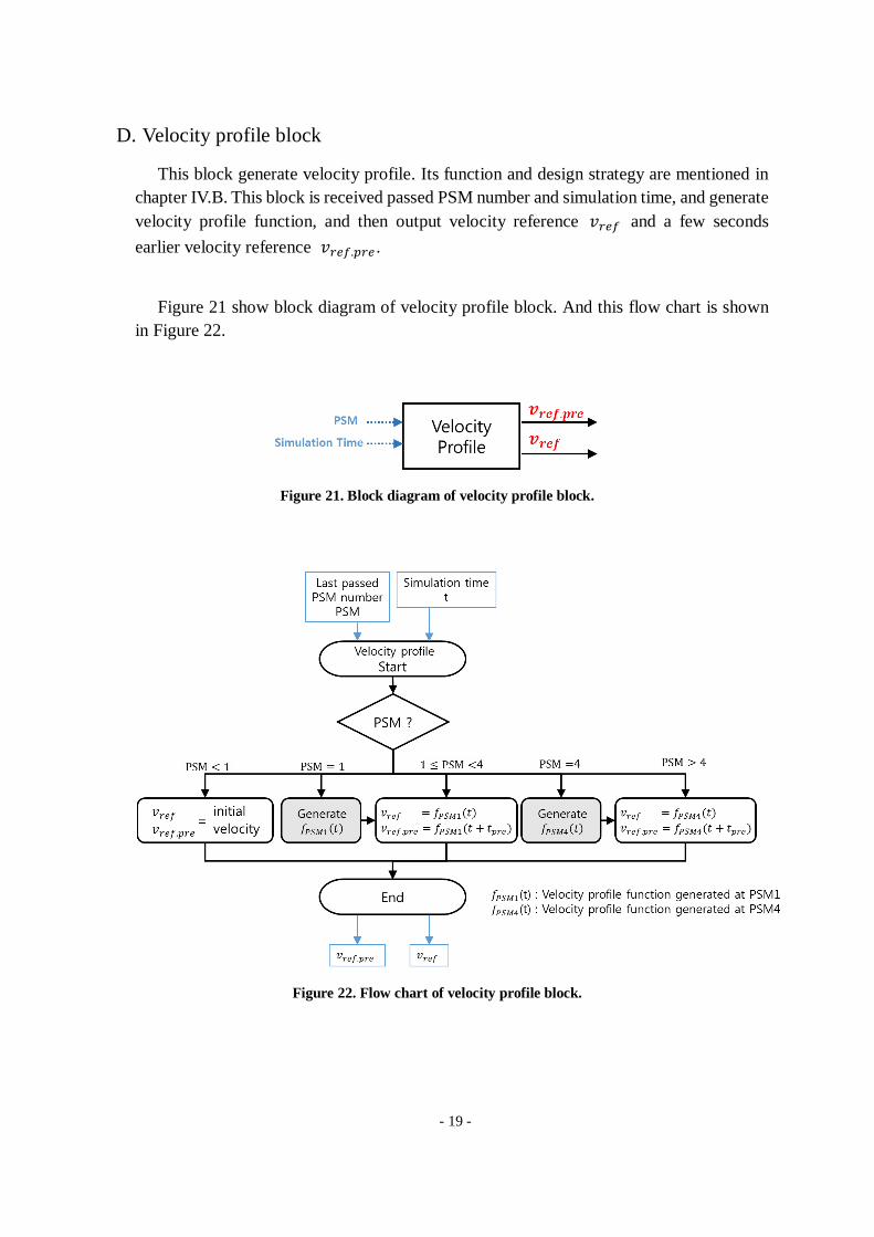
V. Simulator design ............................................................................................................................ - 16 - A. Simulator outline ................................................................................................................... - 16 - B. Six train plant block ............................................................................................................... - 16 - C. Force calculator block ............................................................................................................ - 17 - D. Velocity profile block............................................................................................................. - 19 - E. Mass error estimation algorithm ............................................................................................. - 20 -
VI. Simulation method and result ....................................................................................................... - 23 - A. Simulation method................................................................................................................. - 23 - B. Simulation parameter range .................................................................................................... - 23 - C. Result .................................................................................................................................... - 26 -
VII. Summary and Conclusion ........................................................................................................... - 33 - A. Summary ............................................................................................................................... - 33 - B. Conclusion ............................................................................................................................ - 33 -
References ......................................................................................................................................... - 34 -
iii
List of figures
FIGURE 1. EFFECT OF EXTENDED TRAIN DOORS. ....................................................................................................................- 1 -
FIGURE 2. TRACTION AND BRAKE NONLINEAR CHARACTERISTIC BY TRAIN VELOCITY ......................................................- 4 -
FIGURE 3. TWO KINDS OF TRAIN FORMATION MODEL .........................................................................................................- 5 -
FIGURE 4. LOCATION OF PSM BETWEEN PLATFORMS ..........................................................................................................- 5 -
FIGURE 5. EXAMPLE OF VELOCITY PROFILE..............................................................................................................................- 6 -
FIGURE 6. NUMBER OF N VEHICLE MODEL .............................................................................................................................- 7 -
FIGURE 7. BRAKE TIME DELAY OF AIR BRAKE AND REGENERATIVE BRAKE. .........................................................................- 9 -
FIGURE 8. RUNNING RESISTANCE BY TRAIN VELOCITY. ....................................................................................................... - 10 -
FIGURE 9. BRAKE PRIORITY FOR BLENDING .......................................................................................................................... - 10 -
FIGURE 10. VELOCITY PROFILE TRANSFER VELOCITY V1 TO V2 ......................................................................................... - 12 -
FIGURE 11. A TYPICAL VELOCITY PROFILE BETWEEN PLATFORMS ..................................................................................... - 13 -
FIGURE 12. EXAMPLE OF VELOCITY PROFILE AND TIME SHIFTED VELOCITY PROFILE AFTER PSM1 ............................ - 14 -
FIGURE 13. BLOCK DIAGRAM OF CONTROLLER. .................................................................................................................. - 14 -
FIGURE 14. STEP RESPONSE OF AIR BRAKE AND REGENERATIVE BRAKE WHEN TIME IS 0.9 SECOND. ........................ - 15 -
FIGURE 15. THE SYSTEMS FOLLOW VARIOUS VELOCITY PROFILE ...................................................................................... - 15 -
FIGURE 16. SIMULATOR BLOCK DIAGRAM ............................................................................................................................ - 16 -
FIGURE 17. BLOCK DIAGRAM OF 6 VEHICLES TRAIN MODEL ............................................................................................ - 16 -
FIGURE 18. BLOCK DIAGRAM OF FORCE CALCULATOR BLOCK .......................................................................................... - 17 -
FIGURE 19. FLOW CHART OF FORCE CALCULATOR BLOCK FOR MM TYPE ..................................................................... - 18 -
FIGURE 20. FLOW CHART OF FORCE CALCULATOR BLOCK FOR MT TYPE ....................................................................... - 18 -
FIGURE 21. BLOCK DIAGRAM OF VELOCITY PROFILE BLOCK. ............................................................................................. - 19 -
FIGURE 22. FLOW CHART OF VELOCITY PROFILE BLOCK. ................................................................................................... - 19 -
FIGURE 23. EXAMPLE OF TIME-ACCELERATION GRAPH WHEN MASS ERROR IS OCCURRING 20%. ............................ - 20 -
FIGURE 24. CHARACTERISTIC OF LOW PASS FILTER HLP .................................................................................................... - 21 -
FIGURE 25. BLOCK DIAGRAM OF MASS ERROR ESTIMATION BLOCK ................................................................................ - 21 -
FIGURE 26. FLOW CHART OF MASS ERROR ESTIMATION BLOCK ....................................................................................... - 22 -
FIGURE 27. DISTRIBUTION OF PASSENGERS OVER PLATFORM, WAITING AND BOARDING THE TRAIN ........................ - 24 -
FIGURE 28. RESULT OF SIMULATION OF MM TYPE ............................................................................................................ - 26 -
FIGURE 29. EXAMPLES OF TIME-JERK GRAPH ...................................................................................................................... - 27 -
FIGURE 30. HISTOGRAM OF SIMULATION RESULT ACCORDING TO VARIOUS PARAMETERS COMBINATIONS. ............ - 29 -
FIGURE 31. HISTOGRAM OF SIMULATION RESULT ACCORDING TO VARIOUS PARAMETERS COMBINATIONS WITH
MARKED BY EACH COMPONENT OF MASS ERROR PARAMETER. ............................................................................... - 30 -
FIGURE 32. HISTOGRAM OF SIMULATION RESULT ACCORDING TO VARIOUS PARAMETERS COMBINATIONS WITH
MARKED BY EACH COMPONENT OF BRAKE PURE TIME DELAY PARAMETER. ........................................................... - 31 -
FIGURE 33. HISTOGRAM OF SIMULATION RESULT ACCORDING TO VARIOUS PARAMETERS COMBINATIONS WITH
MARKED BY EACH COMPONENT OF PARAMETER OF VELOCITY AT PSM1. ............................................................. - 32 -
iv
List of tables
TABLE 1. PREVIOUS WORK. ........................................................................................................................................................- 3 -
TABLE 2. PARAMETERS OF EXAMPLE VELOCITY PROFILE ..................................................................................................... - 13 -
TABLE 3. RANGE OF MASS ERROR. ........................................................................................................................................ - 25 -
- 1 -
I. Introduction A. Motivation
In metropolitan, many people use metro train frequently because of its punctuality and
safety. Seoul metro transport 1.5 billion passenger each year [1]. The metro train has been
required more efficiency and safety.
Recently most metro station in Korea have platform screen door (PSD) that divide
passenger space and train track for convenience and safety. Their width is 2 meter. And
current train door width is 1.3 meter that allow two people enter at the same time.
Considering interference between PSDs and train doors, accuracy to the stop should be less
than 0.35 meter. The narrow width of train door can cause traffic jam in rush hour. From
this reason, the Korea Railroad Research Institute (KRRI) consider increasing the train
door size 1.8 meter that can allow three people enter at the same time [2]. In this case
distance of stop error have to be less than 0.1 meter. Figure 1 show effect of extended train
doors. A study on the effect of increasing the door has been fulfilled by the KRRI.
According these recommend, precise stop control become more important. Precise
position stop control make the trains stop at the predefined position of each platform. It
can reduce the interference between PSDs and train doors. And it also reduce train dwell
time.
Figure 1. Effect of extended train doors.
B. Objective
The objective of this study are
1. to establish a train model that represents all the vehicle with its own brake dynamics.
2. to design controller for the precise stop control.
3. to make simulator using the train model with the designed controller.
4. to analyze performance of controller about model parameters.
- 2 -
C. Approach
The approach of this study is described as follows.
1. Train model that is linked 6 vehicles is founded and its state space equation is founded.
In addition, two types of nonlinear brake characteristic that is changed by velocity and
their blending algorithm is reflected.
2. Two types of train formation model are decided. One is one of current formation. In
the formation, half of vehicles have traction motor with two kinds of brakes, and the
other half of vehicles have one kind of brake. The other formation is considered a new
by Korea Railroad Research Institute. All vehicles of the formation have traction
motor with two kinds of brakes.
3. Reference input that is called velocity profile and Controller are designed. The
controller employ feedforward control and PI control.
4. Simulator using the two types of train formation model and designed controller is
designed.
5. Simulation is performed with model parameter that cause model uncertainty. In this
study three parameter is decided: error of passengers’ mass sensing, brake time delay,
entering velocity of stop sequence.
D. Outline
The paper is organized as follows. Chapter Ⅱ presents a background of railroad. In
chapter Ⅲ, a model that include brake nonlinearity and brake time delay and brake
blending algorithm is developed. Chapter Ⅳ describe designing controller and velocity
profile. Chapters Ⅴ and Ⅵ present designing simulator and its result.
- 3 -
II. Background A. Previous work
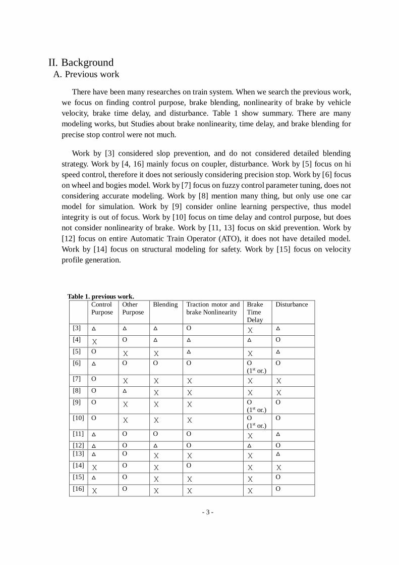
There have been many researches on train system. When we search the previous work,
we focus on finding control purpose, brake blending, nonlinearity of brake by vehicle
velocity, brake time delay, and disturbance. Table 1 show summary. There are many
modeling works, but Studies about brake nonlinearity, time delay, and brake blending for
precise stop control were not much.
Work by [3] considered slop prevention, and do not considered detailed blending
strategy. Work by [4, 16] mainly focus on coupler, disturbance. Work by [5] focus on hi
speed control, therefore it does not seriously considering precision stop. Work by [6] focus
on wheel and bogies model. Work by [7] focus on fuzzy control parameter tuning, does not
considering accurate modeling. Work by [8] mention many thing, but only use one car
model for simulation. Work by [9] consider online learning perspective, thus model
integrity is out of focus. Work by [10] focus on time delay and control purpose, but does
not consider nonlinearity of brake. Work by [11, 13] focus on skid prevention. Work by
[12] focus on entire Automatic Train Operator (ATO), it does not have detailed model.
Work by [14] focus on structural modeling for safety. Work by [15] focus on velocity
profile generation.
Table 1. previous work.
Control
Purpose
Other
Purpose
Blending Traction motor and
brake Nonlinearity
Brake
Time
Delay
Disturbance
[3] △ △ △ O X △
[4] X O △ △ △ O
[5] O X X △ X △
[6] △ O O O O
(1st or.)
O
[7] O X X X X X
[8] O △ X X X X
[9] O X X X O
(1st or.)
O
[10] O X X X O
(1st or.)
O
[11] △ O O O X △
[12] △ O △ O △ O
[13] △ O X X X △
[14] X O X O X X
[15] △ O X X X O
[16] X O X X X O
- 4 -
B. Types of vehicle
The vehicle type in railroad system generally divided two types. One is an M car that
has traction motor. The traction feature is varying as a function of velocity. Traction
motor’s characteristic is shown on Figure 2 (a). And the other is trailer car that is called T
car. It doesn’t have traction motor.
Two types car have different brake systems. Usually M car have two brake system. One
is regenerative brake using traction motor. Its characteristic is like Figure 2 (b). This brake
force is rapidly decrease in low velocity of train. The other is tread brake. It generate brake
force through the pushing wheel by brake shoe using pneumatic pressure. Its characteristic
is shown on Figure 2 (c). In the T car usually have one brake that have large capacity. It is
disk brake that feature is like Figure 2 (d). It generate brake force through the pushing disk
that connect wheel using pneumatic pressure. It is like tread brake. Disk brake and tread
brake have different capacity. Both brake are operated by the air or oil pump. Therefore
this study suppose both time delay feature is same.
Figure 2. Traction and brake nonlinear characteristic by train velocity.
- 5 -
C. Types of train formation
In railroad system, many formation for a train are exist. In this study, two types of train
formation are considered. One is one of current formation like Figure 3 (a). It have three
M cars and three T cars. Thus this formation have three traction motor and three
regenerative brake, and six air brake. It is called MT type for the convenience in this study.
The other formation is considered by the Korea Railroad Research Institute. All vehicles
of this formation is M car like Figure 3 (b). In this study we call it MM type for convenience.
Figure 3. Two kinds of train formation model. (a) MT type, (b) MM type
D. Precision stop marker
In order to detect the accurate position for the train, Precision stop markers (PSM) are
used. There are four markers between platforms like Figure 4. PSM1 is located 546 meters
from stop point. PSM 2~ 4 are located like Figure 4. PSM sensor have measurement error.
It is concerned about train velocity. When train velocity is high, its measurement error is
also large. This study assumes no measurement error of PSM. We do not focus on
localization. This study suppose that distance of train can be measured accurately.
Figure 4. Location of PSM between platforms.
E. Railroad system and velocity profile
Current railroad train can measure own velocity by encoder that is attached wheels.
Displacement is calculated by velocity integral. Therefore velocity is adopted as control
reference in current train system. We suppose that if a train follow velocity reference well,
- 6 -
then the train is well controlled.
In railroad system, it is known that rail information between each station and about
whole section that train service. Thus control reference that called velocity profile is
predefined.
Usually there are many velocity profile for each section based on PSMs in order to
handle various situation. Figure 5 show example of velocity profile.
Figure 5. Example of velocity profile
- 7 -
III. Modeling A. Train model
Many studies suppose train is point mass to represent the train to equation [2, 3]. In this
study, we also suppose one vehicle is point mass and consider a train that have number of
n vehicles, multi-point mass. Figure 6 show number of n vehicles model. The differential
equation is represented in equation 3.1.
𝑝�̇� = 𝑣𝑖
𝑚𝑖𝑣�̇� = 𝑘𝑖−1(𝑝𝑖−1 − 𝑝𝑖) + 𝑘𝑖(𝑝𝑖+1 − 𝑝𝑖) + 𝑐𝑖−1(𝑣𝑖−1 − 𝑣𝑖) + 𝑐𝑖(𝑣𝑖+1 − 𝑣𝑖) + 𝐹𝑖(𝑣𝑖) (3.1)
Fi(𝑣𝑖) = 𝐹𝑖,𝑡𝑟𝑎𝑐𝑡𝑖𝑜𝑛(𝑣𝑖) + 𝐹𝑖,𝑟𝑒𝑔.𝑏𝑟𝑎𝑘𝑒(𝑣𝑖) + 𝐹𝑖,𝑎𝑖𝑟.𝑏𝑟𝑎𝑘𝑒(𝑣𝑖) + 𝐹𝑖,𝑑𝑟𝑎𝑔(𝑣𝑖)
In above equation mi, 𝑝𝑖 , 𝑣𝑖 is 𝑖 th vehicle’s mass, position, velocity respectively. And ki, 𝑐𝑖
is spring constant and damping constant of coupler between 𝑖 th vehicle and 𝑖 + 1 th vehicle.
And 𝐹𝑖 is 𝑖 th vehicle’s sum of traction force 𝐹𝑖.𝑡𝑟𝑎𝑐𝑡𝑖𝑜𝑛 , brake force 𝐹𝑖,𝑟𝑒𝑔.𝑏𝑟𝑎𝑘𝑒 + 𝐹𝑖,𝑎𝑖𝑟.𝑏𝑟𝑎𝑘𝑒
and running resistance 𝐹𝑖.𝑑𝑟𝑎𝑔 .
This study decide ki, 𝑐𝑖 is 3.4 × 10⁶N/m, 8333 N*sec/m respectively by [17],[18].
Figure 6. Number of n vehicle model.
According to equation 3.1, state space equation of six vehicles train can be found as follow.
�̇� = 𝐴𝑥 + 𝐵 [𝐹1⋮𝐹6
] , 𝑦 = 𝐶𝑥, 𝑥 =
[ 𝑝1𝑣1⋮𝑝6𝑣6]
(3.2)
𝐴 =
[ 𝑅𝑏1𝑅𝑎202×202×202×202×2
𝑅𝑐1𝑅𝑏2𝑅𝑎302×202×202×2
02×2𝑅𝑐2𝑅𝑏3𝑅𝑎402×202×2
02×202×2𝑅𝑐3𝑅𝑏4𝑅𝑎502×2
02×202×202×2𝑅𝑐4𝑅𝑏5𝑅𝑎6
02×202×202×202×2𝑅𝑐5𝑅𝑏6 ]
𝑅𝑎𝑖 = [0 0𝑘𝑖−1
𝑚𝑖
𝑐𝑖−1
𝑚𝑖
], 𝑅𝑏𝑖 = [0 0
−𝑘𝑖−1−𝑘𝑖
𝑚𝑖
−𝑐𝑖−1−𝑐𝑖
𝑚𝑖
] , 𝑅𝑐𝑖 = [0 0𝑘𝑖
𝑚𝑖
𝑐𝑖
𝑚𝑖
]
- 8 -
𝐵 =
[ 0 0 0 0 0 01
𝑚10 0 0 0 0
0 0 0 0 0 0
01
𝑚20 0 0 0
0 0 0 0 0 0
0 01
𝑚30 0 0
0 0 0 0 0 0
0 0 01
𝑚40 0
0 0 0 0 0 0
0 0 0 01
𝑚50
0 0 0 0 0 0
0 0 0 0 01
𝑚6]
𝐶 =
[ 0 1 0 0 0 0 0 0 0 0 0 00 0 0 1 0 0 0 0 0 0 0 00 0 0 0 0 1 0 0 0 0 0 00 0 0 0 0 0 0 1 0 0 0 00 0 0 0 0 0 0 0 0 1 0 00 0 0 0 0 0 0 0 0 0 0 1]
In order to simplify model, we assume straight and plain track. Thus this study does not
consider track gradient resistance and track curve resistance. Both are small that can be
ignored around the stop point.
B. Brake time delay
One of important feature of brake is time delay. Brake time delay can divided into pure
delay and transient response. This study consider three types brake. Two of them is air
brake that is operated by pneumatic process. Their brake time delay are almost same. The
other one is a regenerative brake operated by electrical process. Its response is much faster
than air brake. Figure 7 show step response of air brake and regenerative brake [2]. It can
be represented by follow equation.
𝐻𝑟𝑏 = 𝑒−0.2𝑠 ∗
6.92
𝑠2+(2×6.9)𝑠+6.92 (3.3)
𝐻𝑎𝑏 = 𝑒−0.2𝑠 ∗
2.32
𝑠2+(2×2.3)𝑠+2.32 (3.4)
- 9 -
Figure 7. Brake time delay of air brake and regenerative brake.
C. Running resistance
In a real railroad system, many disturbances are existing. Among them, there are more
notable. The most representative disturbances are three things: track gradient resistance,
track curve resistance and running resistance. We have known information about track
gradient and track curve in advance. Thus we can handle the resistances about them and
cancel out. Here, we assume straight and plain track for the simplicity. Therefore the
gradient resistance and curve resistance can be ignored around stop point.
Running resistance is sum of wheel rolling resistance and air resistance. It is usually
hard to analyze mathematically and founded experimentally [19]. In this study, it is
approximated by second order polynomial as follow. It is based on experimental data from
the KRRI.
𝑓𝑑(𝑣) = 𝑚 × (0.022𝑣2 + 0.036|𝑣| + 0.961) × 10−3 (3.5)
In this equation, 𝑣 is velocity of vehicle, and m is mass of train. According to [19],
air resistance of running resistance is proportional to square of velocity of head vehicle.
This study consider six vehicles train. Thus the head vehicle applied following equation
(3.6), and the other vehicles applied following equation (3.7)
𝑓𝑑𝑟𝑎𝑔1(𝑣1) = 𝑚1 × (0.022𝑣2 + 0.036|𝑣| + 0.961) × 10−3 (3.6)
𝑓𝑑𝑟𝑎𝑔2(𝑣𝑖) = 𝑚𝑖 × (0.036|𝑣| + 0.961) × 10−3, i = 2, 3, 4, 5, 6 (3.7)
Figure 8 show resistance by train velocity. Blue line show 𝑓𝑑𝑟𝑎𝑔1 and read line show
𝑓𝑑𝑟𝑎𝑔2.
- 10 -
Figure 8. Running resistance by train velocity.
D. Brake blending
Train has several brakes that denote different characteristics according to the velocity.
Therefore strategy of how to use those brakes is one of main issue in the railroad system.
This study adopt priority brake strategy that is commonly considered. It is represented
in Figure 9. In MT type, when operator command braking, the train use regenerative brake
of M car first. If its force is saturated that mean regenerative brake for is not enough, the
train begin to use air brake of T car. If the air brake of T car is also saturated, the train start
to use air brake of M car sequentially. The strategy for the MM type is similar, except that
it skips the T car air brake. Train use regenerative brake first, and then if its force is not
enough, the train begin to use air brake.
The reason of using regenerative brake first is to extend life time of air brakes. The air
brakes generate brake force from physical friction. And the regenerative brake get brake
force from electrical resistance. Thus, reducing usage of air brakes can extend life time of
train.
Figure 9. Brake priority for blending. (a) MT type, (b) MM type
0 5 10 15 20 25 300.5
1
1.5
2
2.5
3
3.5x 10
-3 Running Resistance(fd)
Velocity(m/s)
Resis
tance(k
gf/
kg)
first car
other car
- 11 -
IV. Velocity profile and controller design A. Control strategy
Usually control reference of train is velocity that is called velocity profile. It is
predefined value that is based on each geological track information between stations. It is
same that the control references are predefined. It means that we know control reference
about entire track before the train operate. In this case, feedforward control is one of
suitable control strategy. The feedforward control generate command signal by predefined
value or detected disturbance in advance. In railroad system velocity profile is predefined
value. The general tracking system doesn’t have predefined control reference, but railroad
system have it. Therefore this study adopt feedforward control to precise stop control of
train.
The feedforward control is not based on error that is between system output and control
reference. Thus in order to adjust system error, we add proportional-integral (PI) control.
Most amount of control value is decided by feedforward control, and remained control
value is handled by PI control.
In this study, we assume that train does not use traction when the train is in stopping
sequence in order to consider energy efficiency. This limitation is kind of actuator
saturation. Thus it cause wind-up phenomenon of I control (integral control). To take care
of wind-up phenomenon this study apply anti wind-up control to PI control.
Lastly brake time delay have to be considered. In order to reduce influence of brake
time delay, this study use time shift of the feedforward control input signal. We generated
a few seconds earlier velocity reference, and put it to feedforward input. In order to apply
this method, an appropriate velocity profile function is generated as follows.
B. Velocity profile design
Velocity profile is control reference, and it does not have formulaic policy. But it have
to be considered ride comfort and train specifications [2, 15].
Ride comfort is associated with jerk that is a derivative of acceleration of train. The
maximal jerk value specified by [2] is 0.8 m/s3 to maintain good passengers’ ride
comfort. And the other factor we have to consider is train specifications. Every real
actuator have limitation. Train also have maximum acceleration and deceleration due to
the capacity of the traction motor and brake. This study develop velocity generating
method from the [2, 15]. It is concerned about jerk limit and maximum deceleration. The
velocity profile equation made by second order polynomial function.
First, it is considered a situation that transfer velocity 𝑣1 to 𝑣2 under fixed maximum
jerk and fixed maximum acceleration. Figure 10 show the velocity profile about this
- 12 -
situation. Equations are described as follows.
∆𝑣 = 𝑣1 − 𝑣2
𝑗 =𝑗𝑚
∆𝑣
𝑎 =𝑎𝑚
∆𝑣
𝛼 =𝑎
𝑗=
𝑎𝑚
𝑗𝑚 (3.8)
𝛽 =∆𝑣
𝑗𝑚×𝛼− 𝛼 (3.9)
∆𝑃2𝛼𝛽 = (𝑣1(2𝛼 + 𝛽)) − (1
2𝑗𝑚𝛼
2(𝛼 + 𝛽) +1
2𝑗𝑚𝛼𝛽
2 + (1
2𝑗𝑚𝛼
2 + 𝑗𝑚𝛼𝛽)𝛼)
𝑣1𝛾 + ∆𝑃2𝛼𝛽=∆𝑃
𝛾 =∆𝑃−∆𝑃2𝛼𝛽
𝑣1 (3.10)
𝑤(𝑡) =
{
0 , 𝑡0 < 𝑡 < 𝑡0 + 𝛾1
2𝑗(𝑡 − 𝑡0 − 𝛾)
2 , 𝑡0 + 𝛾 < 𝑡 < 𝑡0 + 𝛾 + 𝛼
j𝛼(𝑡 − 𝑡0 − 𝛾 − 𝛼) +1
2𝑗𝛼2 , 𝑡0 + 𝛾 + 𝛼 < 𝑡 < 𝑡0 + 𝛾 + 𝛼 + 𝛽
−1
2𝑗(𝑡 − 𝑡0 − 𝛾 − 2𝛼 − 𝛽)
2 + (𝑗𝛼2 + 𝑗𝛼𝛽) , 𝑡0 + 𝛾 + 𝛼 + 𝛽 < 𝑡 < 𝑡0 + 𝛾 + 2𝛼 + 𝛽
𝑣(𝑡) = 𝑣1𝑤(𝑡) − 𝑣2(1 − 𝑤(𝑡)) (3.11)
Firstly, we assign start velocity 𝑣1, end velocity 𝑣2, maximum jerk jm , maximum
deceleration ( or acceleration) am, and moving distance ∆P. Then each section time 𝛼, 𝛽,
and 𝛾 can be calculated according to the above equation. And velocity profile 𝑣(𝑡) can
be found.
Figure 10. Velocity profile transfer velocity 𝒗𝟏 to 𝒗𝟐
- 13 -
A typical velocity profile between two stations is shown in Figure 11. There are three
sections in the velocity profile. Those are traction, brake1, and brake2 section respectively.
And each sections parameter is describe in Table 2.
In order to consider brake time delay, the control strategy is to generate a few seconds
earlier velocity profile for feedforward control input. To generate a few seconds earlier
velocity profile, the equation (3.11) is shifted with a constant time 𝑡𝑝𝑟𝑒 as follows.
𝑣(𝑡 + 𝑡𝑝𝑟𝑒) = 𝑣1𝑤(𝑡 + 𝑡𝑝𝑟𝑒) − 𝑣2(1 − 𝑤(𝑡 + 𝑡𝑝𝑟𝑒)) (3.12)
Figure 12 show example of velocity profile and 𝑡𝑝𝑟𝑒 second earlier velocity profile.
Figure 11. A typical velocity profile between platforms. (a) Velocity profile diagram, (b) Velocity profile
made by Matlab.
Table 2. Parameters of example velocity profile
Traction Brake 1 Brake2
Start velocity 𝒗𝟏 (𝒎/𝒔) 0 19.4 1.2
End velocity 𝒗𝟐 (𝒎/𝒔) 19.4 1.2 0
𝒋𝒎 (𝒎/𝒔𝟐) 0.5 0.5 0.5
𝒂𝒎 (𝒎/𝒔𝟑) 0.5 1 0.5
∆𝑷
(𝒎𝒆𝒕𝒆𝒓)
Stop point ~
PSM1
PSM1 ~
(PSM4 - 1 meter)
PSM4~
Stop point
- 14 -
Figure 12. Example of velocity profile and time shifted velocity profile after PSM1.
C. Controller design
Figure 13 is block diagram of designed controller that uses feedforward control and PI
control. The input to the feedforward control is the velocity profile 𝑣𝑟𝑒𝑓.𝑝𝑟𝑒 which is
represented in (3.12). The shift time 𝑡𝑝𝑟𝑒 is found by try and error method when only
feedforward controller connect to whole simulator. This study decide it 0.9 second. Figure
14 show step response of two types of brake time delay when time is 0.9 second. And PI
controller gain and anti-windup gain also are found by try and error method. Proportional
gain (kp) is 2, integral gain (ki) is 0.5, and anti-windup gain (ka) is 0.5.
Figure 13. Block diagram of controller.
- 15 -
Figure 14. Step response of air brake and regenerative brake when time is 0.9 second.
D. Controller stability
The train model this study considers has actuator time delay and brake nonlinear factors.
The actuator time delay is divided into traction motor time delay, regenerative brake time
delay, and air brake time delay. The amount of three delays are different from each other.
The delays for the brakes and the delay for the motor are different leading to asymmetric
delay in the actuation of control systems. Actuator asymmetric characteristics is hard to
mathematically analyze stability. The first attempt is to divide two systems which are
traction system and brake system. And switched systems theory of [20, 21] is applied. This
approach verification could not yet complete. It will be one of our future work. Another
approach is to show that the system can be able to track closely various velocity references.
Figure 15 shows that the system track various velocity closely.
Figure 15. The systems follow various velocity profile. (a) MT type, (b) MM type
- 16 -
V. Simulator design A. Simulator outline
The simulator is composed of blocks as shown in Figure 16 (a). The simulator is
implemented with MATLAB Simulink as shown in Figure 16 (b). The structure and the
functions of each block in the simulator will be described in this chapter.
Figure 16. Simulator block diagram. (a) Simulator block diagram, (b) whole simulator block of Matlab
Simulink
B. Six train plant block
The train model state equation is represented in chapter III.A. and equation (3.2). This
block is made by state space library of Matlab Simulink and stop brake block which is
imaginary brake in order to reduce system complexity and avoid numerical error in the
Matlab. In this study we suppose that train is stopped once velocity is less than zero. The
six train plant block diagram is represented in Figure 17.
Figure 17. Block diagram of 6 vehicles train model.
- 17 -
C. Force calculator block
This block calculate force of each vehicle from demanded acceleration (or deceleration)
and current velocity of the vehicle. The force is sum of traction force, brake forces, and
drag force. The traction force that traction motor generate is multiplication of demanded
acceleration and mass of vehicle. And it has maximum force 𝑓𝑣(𝑣) that is according to
their velocity as shown in Figure 2. (a). The brake forces that is generated by regenerative
brake and air brakes are multiplication of demanded deceleration and mass of vehicle. And
it also has maximum forces 𝑓𝑟𝑏(𝑣), 𝑓𝑎𝑏(𝑣) and 𝑓𝑇,𝑎𝑏(𝑣) respectively that is according
to their velocity as shown in Figure 2. (b), (c), (d). And the brake forces have different
brake blending algorithm according to train type (MM type or MT type) that is mentioned
in chapter III.D. The drag force is running resistance that is mentioned in chapter III.C.
The head vehicle's drag force is followed equation (3.6), and the other vehicles are
followed equation (3.7).
Figure 18 show block diagram of force calculator block for MM type and MT type.
Their flow chart is shown in Figure 19 and Figure 20 respectively.
Figure 18. Block diagram of force calculator block. (a) MM type, (b) MT type
- 18 -
Figure 19. Flow chart of force calculator block for MM type. The 𝒇𝒕(𝒗), 𝒇𝒓𝒃(𝒗), 𝒇𝒂𝒃(𝒗) are mentioned in
chapter II.B. 𝒇𝒅𝒓𝒂𝒈𝟏(𝒗), 𝒇𝒅𝒓𝒂𝒈𝟐(𝒗) are mentioned in equation (3.6) and (3.7)
Figure 20. Flow chart of force calculator block for MT type. The 𝒇𝒕(𝒗), 𝒇𝒓𝒃(𝒗), 𝒇𝒂𝒃(𝒗) are mentioned in
chapter II.B. 𝒇𝒅𝒓𝒂𝒈𝟏(𝒗), 𝒇𝒅𝒓𝒂𝒈𝟐(𝒗) are mentioned in equation (3.6) and (3.7)
- 19 -
D. Velocity profile block
This block generate velocity profile. Its function and design strategy are mentioned in
chapter IV.B. This block is received passed PSM number and simulation time, and generate
velocity profile function, and then output velocity reference 𝑣𝑟𝑒𝑓 and a few seconds
earlier velocity reference 𝑣𝑟𝑒𝑓.𝑝𝑟𝑒 .
Figure 21 show block diagram of velocity profile block. And this flow chart is shown
in Figure 22.
Figure 21. Block diagram of velocity profile block.
Figure 22. Flow chart of velocity profile block.
- 20 -
E. Mass error estimation algorithm
Before train start from the station, the train measure passenger weight by measuring the
reduce size of the spring. There exist measurement error. This section try to compensate
for passenger mass error.
In this study, six vehicles are connected by coupler. Therefore, estimation of each
vehicle mass error is hard to implement. Thus this study make an attempt to estimate whole
mass error of train, where the train is in uniformly accelerated motion. In uniformly
accelerated section, controller output and acceleration of the lead car is same when there
are no mass error. But if the mass error is existed, they could have different value. their
error is constant value. Velocity profile mentioned in chapter IV.B have uniformly
accelerated section 𝛽. Figure 23 is represented controller output and acceleration of lead
car when mass error is occurring 20%.
Figure 23. Example of time-acceleration graph when mass error is occurring 20%.
Before the implement, we suppose that brakes of train do not saturate. First, this study
estimate mass error. In uniformly accelerated section, controller output 𝐹𝑐 and force of
train 𝐹𝑡𝑟𝑎𝑖𝑛 are same. Using this, we can calculate mass error 𝑚𝑒 as follows.
𝐹𝑐 = 𝑚𝑐𝑎𝑐 (5.1)
𝐹𝑡𝑟𝑎𝑖𝑛 = (𝑚𝑐 +𝑚𝑒)𝑎𝑜𝑢𝑡 (5.2)
𝐹𝑐 = 𝐹𝑡𝑟𝑎𝑖𝑛
𝑚𝑒 =(𝑎𝑐−𝑎𝑜𝑢𝑡)𝑚𝑐
𝑎𝑜𝑢𝑡 (5.3)
In here, 𝑚𝑐 is mass value the controller know, and 𝑎𝑐 is control output, 𝑎𝑜𝑢𝑡 is
acceleration of train. And next, the estimated mass error is applied to the system. Strategy
is that the estimated mass error convert to additional control value as follows.
𝐹𝑐.𝑒𝑠𝑡 = (𝑚𝑐 +𝑚𝑒)𝑎𝑐 = 𝑚𝑐(𝑎𝑐 + 𝑎𝑚𝑒𝑒) (5.4)
- 21 -
𝐹𝑡𝑟𝑎𝑖𝑛.𝑒𝑠𝑡 = (𝑚𝑐 +𝑚𝑒)𝑎𝑜𝑢𝑡 (5.5)
𝑎𝑚𝑒𝑒 =𝑚𝑒
𝑚𝑐𝑎𝑐 (5.6)
In the above equation, 𝐹𝑐.𝑒𝑠𝑡, 𝐹𝑡𝑟𝑎𝑖𝑛.𝑒𝑠𝑡 are estimated controller output and estimated
train output force by estimated mass error. 𝑎𝑚𝑒𝑒 is additional control value according to
estimated mass error.
Before implementing this algorithm to the simulator. In order to remove a noise of
control output and train output value that is input of mass error estimation block, we use
second order low pass filter. Because the values are DC value in uniformly accelerated
section, cut off frequency of the filter is small value. The filter specification is as follows.
Cut off frequency is 0.7 Hz that is decided by try and error method, and it is designed by
second order Butterworth filter. This study use butter function of Matlab. The filter
equation is follows. And its characteristic is shown by Figure 24.
Hlp(S) =0.49
𝑠2+0.9899𝑠+0.49 (5.7)
Figure 24. Characteristic of low pass filter 𝑯𝒍𝒑. (a) Step response, (b) Frequency response.
The mass error estimation algorithm is implemented in mass error estimator block. Its
block diagram is represented in Figure 25. And its flow chart is shown in Figure 26.
Figure 25. Block diagram of mass error estimation block.
- 23 -
VI. Simulation method and result A. Simulation method
Before starting simulation, this study decide simulation object and simulation parameter.
Four simulation object is decided as follows,
Object 1. MT type
Object 2. MT type + mee : MT type applied mass error estimation algorithm.
Object 3. MM type
Object 5. MM type + mee : MM type applied mass error estimation algorithm.
Three simulation parameter is decided as follow,
Parameter 1. Mass error
Parameter 2. Brake pure time delay.
Parameter 3. Velocity at PSM1 that is starting point of stopping sequence.
Simulation is implemented after the train entering the PSM1 until stopped according to
various parameter combinations. Parameter range is as follows.
B. Simulation parameter range
1. Mass error
This is the situation that passenger weight sensing sensor occur measurement error. Two
kinds of scenario is considered.
The first scenario is considered that passengers converge on specific platform. Work by
[22] research this situation. Figure 27 show example of Distribution of passengers over
platform. In order to reflect this scenario, this paper suppose that one vehicle has mass
error.
The second scenario is considered rush hour. In rush hour passengers are increased. In
this case, weight of train is also increased too. In order to reflect his scenario, we suppose
that whole vehicle have mass error.
The range of mass error is represented by Table 3.
- 24 -
Figure 27. Distribution of passengers over platform, waiting and boarding the train. (a) is case of The
Hague, (b) is case of Tilburg, (c) is case of Eindhoven. [22]
- 25 -
Table 3. Range of mass error.
Category Error (%)
(car1,car2,car3,car4,car5,car6) case
One vehicle
has mass error
(-30% ~ 30%,
interval 10%)
(xx,0,0,0,0,0)
(0, xx,0,0,0,0)
(0,0, xx,0,0,0)
(0,0,0, xx,0,0)
(0,0,0,0, xx,0)
(0,0,0,0,0, xx)
36
Whole vehicles
have mass error
(-30% ~ 30%,
interval 10%)
(xx,xx,xx,xx,xx,xx) 6
0% Mass error (0,0,0,0,0,0) 1
2. Brake pure time delay
This is for situation that time delay is different between real train and value that
controller know. This study just consider pure delay to reduce simulation complexity.
Decided time delay are 0.1, 0.2, 0.3, 0.4 second.
3. Velocity at PSM1 that is starting point of stopping sequence
This study goal is stop control. Therefore the simulate start at the PSM1 that is started
sopping sequence. In order to confirm effect of velocity at PSM1, it is decided simulation
parameter.
Decided parameter of velocity at PSM1 are 60, 70, 80 km/h.
- 26 -
C. Result
1. Simulation results and their indicators.
When this study figure out the controller gain, the simulation parameter that is standard
is as follow. Mass error is zero, brake time delay is 0.2s, velocity at PSM1 is 70km/s. In
this case, simulation result is shown in Figure 28. Its stop error is about 3 cm. and jerk
values are shown under 0.5 𝑚/𝑠3. There are satisfy the specification that stop error is less
than 10 cm, jerk is less than 0.8 𝑚/𝑠3.
The parameter combination is 516 case per each object. Therefore indicator value have
to be decided. This study decided three indicator: stop error, jerk RMS, stop time.
a. Stop error: it is the first car’s stop distance error
b. Jerk RMS (Root mean square): it is the first car’s jerk RMS value. Figure 29 show examples
of jerk RMS value. Less than 0.15 is good ride quality, and over 0.45 is bad ride quality.
c. Stop time: it is simulation time when train is stopped.
Figure 28. Result of simulation of MM type when mass error is 0%, brake time delay is 0.2s, velocity at
PSM1 is 70km/h.
- 27 -
Figure 29. Examples of time-jerk graph. (a) MM type, mass error is 0%, brake time delay is 0.1s, velocity
at PSM1 is 60km/h, (b) MM type, mass error is whole vehicles have -30%, brake time delay is 0.4s,
velocity at PSM1 is 70km/h, (c) MT type, mass error is only third vehicle have 20%, brake time delay is
0.1s, velocity at PSM1 is 90km/h
2. Histogram of simulation result
The parameter combination is 516 case per each object. Therefore simulation result is
represented by histogram. Histograms’ detail setting is as follows.
In histogram of stop error, stop error interval is 0.5 cm, range is from -20 cm to 20 cm.
The number of results of over upper bound is displayed at 20 cm, and the number of results
of under the lower bound is displayed at -20 cm.
In histogram of jerk RMS, jerk RMS interval is 0.005, range is from 0 to 0.55. The
number of results of over upper bound is displayed at 0.55, and the number of results of
under the lower bound is displayed at 0.
In histogram of stop time, stop time interval is 0.05 second, range is from 40 to 47
second. The number of results of over upper bound is displayed at 40 second, and the
number of results of under the lower bound is displayed at 47 second.
- 28 -
3. Integrated result analysis
Figure 30 is result according to every various parameters combinations for each object.
According to stop error histogram, it can be confirmed that MM type’s stop error is
smaller than MT type, and mass error estimation algorithm show evident performance
improvement about stop distance error.
According to jerk RMS histogram, it can be confirmed that MM type’s ride quality is
much better than MT type about uncertain factors. In this case, mass error estimation
algorithm does not contribute much.
According to stop time histogram, it can be confirmed that MM type and MT type are
show similar stop time, and through the mass error estimation algorithm, stop time
scattering can be short.
4. Result analysis according to mass error parameters
Figure 31 represent ingredients of mass error parameters on Figure 30.
According to jerk RMS histogram, MM type is robust about mass error, but MT type
occur huge jerk when one vehicle have mass error.
Stop error is increased when the train has large mass error.
The mass error parameter does not have a specific impact to stop time.
5. Result analysis according to brake pure time delay parameters
Figure 32 represent ingredients of time delay parameters on Figure 30
According to stop error histogram, the brake time delay parameter have a great effect
on stop error. When it is increased, the stop error is also increase specifically.
6. Result analysis according to brake velocity at PSM1 parameter.
Figure 33 represent ingredients of velocity at PSM1 parameters on Figure 30
According to stop time histogram, the velocity at PSM have a great effect on stop time.
When it is increase, the stop time is decrease clearly.
- 30 -
Figure 31. Histogram of simulation result according to various parameters combinations with marked by
each component of mass error parameter.
- 31 -
Figure 32. Histogram of simulation result according to various parameters combinations with marked by
each component of brake pure time delay parameter.
- 32 -
Figure 33. Histogram of simulation result according to various parameters combinations with marked by
each component of parameter of velocity at PSM1.
- 33 -
VII. Summary and Conclusion
A. Summary
In order to satisfy requirements of precision stop, this study develop model of
metropolitan train and suitable controller with simulator. The model of train is considered
formation, brake nonlinearity, and brake blending. The controller used feedforward control
and PI control with anti-wind up. The control reference that is called velocity profile is
developed according PSM markers. In addition, to reduce effect of passenger mass
measurement error, mass error estimation algorithm is suggested and applied. Simulation
is implemented about two kinds of formation which one is current formation (MT type),
the other is next version (MM type). In the result, new formation show much better
performance, and mass error estimation algorithm is showed improved performance.
B. Conclusion
In this study designed model and controller for metropolitan train. It is confirmed that
Feedforward control with PI control is suitable to control the railroad system. And some
of parameter can be effect on stop distance and ride quality. This study confirm that the
train formation can be significant effect on ride quality. And brake time delay can be
significant effect on stop distance error. In addition, according to estimate mass error
method, improvement of stop error is confirmed.
- 34 -
References
[1] Seoul metro, (2014), http://www.seoulmetro.co.kr
[2] KRRI, (2013), “Study on the rapidization for the metro transit system and
the related compatible functions ”, KRRI 2013-006 (ISBN: 978-89-97667-20-8)
[3] H. A. Ahmad, (2013),"Dynamic Braking Control for Accurate Train Braking Distance Estimation
under Different Operating Conditions," Virginia Polytechnic Institute and State University.
[4] S. Iwnicki, (2006),Handbook of railway vehicle dynamics: CRC press.
[5] Q. Song, Y. Song, and W. Cai, (2011),"Adaptive backstepping control of train systems with
traction/braking dynamics and uncertain resistive forces," Vehicle System Dynamics, vol. 49, pp. 1441-
1454.
[6] C.-G. Kang, (2007),"Analysis of the braking system of the Korean high-speed train using real-time
simulations," Journal of Mechanical science and Technology, vol. 21, pp. 1048-1057.
[7] D. Chen and C. Gao, (2012),"Soft computing methods applied to train station parking in urban rail
transit," Applied Soft Computing, vol. 12, pp. 759-767.
[8] Q. Song, Y.-d. Song, T. Tang, and B. Ning, (2011),"Computationally inexpensive tracking control of
high-speed trains with traction/braking saturation," Intelligent Transportation Systems, IEEE
Transactions on, vol. 12, pp. 1116-1125.
[9] D. Chen, R. Chen, Y. Li, and T. Tang, (2013),"Online learning algorithms for train automatic stop
control using precise location data of balises,".
[10] Z.-Y. Yu and D.-W. Chen, (2011),"Modeling and system identification of the braking system of
urban rail vehicles," Journal of the China railway Society, vol. 33, pp. 37-40.
[11] K. Teramoto, K. Ohishi, T. Kondo, S. Makishima, K. Uezono, and S. Yasukawa, (2014),"Electro-
pneumatic Blended Braking Control of Regenerative Brake and Air Brake based on Estimated Adhesion
Coefficient," IEEJ Journal of Industry Applications, vol. 3, pp. 75-85.
[12] H. Dong, B. Ning, B. Cai, and Z. Hou, (2010),"Automatic train control system development and
simulation for high-speed railways," IEEE circuits and systems magazine, vol. 10, pp. 6-18.
[13] H. Yamazaki, Y. Karino, M. Nagai, and T. Kamada, (2005),"Wheel Slip Prevention Control by
Sliding Mode Control for Railway Vehicles(Experiments Using Real Size Test)," in Advanced Intelligent
Mechatronics. Proceedings, 2005 IEEE/ASME International Conference on, pp. 271-276.
[14] Joon-Hyuk Park, Byeong-Choon Goo, (2007),"Dynamic Modeling of a Railway Vehicle under
Braking" The Korean Society for Railway, vol. 10, pp. 431-437.
[15] Taeyeon Lee et al., (1999),"The selection of ATO profile on precision stop controller for urban
railway" Journal of he Korean Society for Railway, pp. 251-258.
[16] H. Zhiwu, T. Haitao, and F. Yanfen, (2010),"The Longitudinal Dynamics of Heavy-Haul Trains in
the Asynchronous Brake Control System," in Measuring Technology and Mechatronics Automation
(ICMTMA), 2010 International Conference on, pp. 900-903.
[17] YUJIN machinery Ltd., (2008), “다중 연결기(제품 규격서)”, document number:RPs-CP1-B19K
[18] Roaduser International Pty Ltd, (2000), “IN-SERVICE ASSESSMENT OF ROAD-FRIENDLY
SUSPENSIONS”, Report for Australian National Road Transport Commission.
[19] 이하라 가즈오, (2012), 철도차량 메커니즘 도감, 골든벨
[20] Daniel Liberzon and A. Stephen Morse, (1999), “Basic Problems in Stability and Design of Switched
Systems”, Control Systems, IEEE, vol. 10, pp.59-70.
[21] M.Wicksl, P. Peleties and R.DeCarlo, (1998), “Switched Controller Synthesis for the Quadratic
Stabilisation of a Pair of Unstable Linear Systems”, European Journal of Control, vol. 4, pp.140-147.
[22] Ir. Paul B.L. Wiggenraad, (2001), “Alighting and boarding times of passengers at Dutch railway
stations”, TRAIL Research School
- 35 -
요 약 문
도시철도 정위치 정차 제어를 위한 열차 모델링과 제어기 및
시뮬레이터 개발
도시철도의 정위치 정차 제어는 열차가 각 플랫폼의 정해진 위치에 정확히
정차 하도록 하는 기술로 열차의 안전성과 정시성을 향상시키고 플랫폼에 설치된 스크린
도어와의 간섭을 최소화 하는 역할을 한다. 정위치 정차에 영향을 미치는 요소는 열차의
편성, 각 열차에 사용된 브레이크의 종류, 브레이크의 비선형 특성, 속도 프로파일, 각종
센서들의 오차 등이 있다. 본 논문에서는 2가지 종류의 6량 열차 편성과 브레이크의
비선형 특성을 반영하여 열차를 모델링 하였다. 제어기 디자인에서는 제어기의 레스펀스
입력인 속도 프로파일을 사전에 알고 있는 특징과 브레이크의 시간 지연 특징을 고려하여
Feedforward 와 PI control 을 이용한 제어기를 디자인 하였다. 또한 승객의 무게를
측정하는 응하중 센서의 오차, 브레이크의 시간지연의 정도, 정지 동작을 시작 할 때의
진입 속도, 이 3가지 모델 파라미터를 변경하며 제어기나 각각의 열차 편성 성능을 분석
할 수 있는 시뮬레이터를 디자인 하여 적용하였다. 이 시뮬레이터를 통해 디자인한
제어기와 열차 편성 변화에 따른 정차 위치 오차, 승차감, 정차 시간을 확인하고 성능
해석을 하였다. 시뮬레이션 결과 열차의 정차 오차는 모델 파라미터에 오차가 있어도
수용할 만한 성능을 보였다. 이를 통해 도시철도의 정차 제어 성능 향상과 실제 시스템에
적용하기 위한 실차 실험의 기간 단축과 비용 절감을 기대 한다.
핵심어: 도시철도, 정위치 정차 제어, 열차 브레이크 모델, 속도프로파일, Feedforward.