MODELING AND SIMULATION OF A HYDROCRACKING UNITjestec.taylors.edu.my/Vol 11 issue 6 June...

Journal of Engineering Science and Technology Vol. 11, No. 6 (2016) 881 - 898 © School of Engineering, Taylor’s University

881

MODELING AND SIMULATION OF A HYDROCRACKING UNIT

HASSAN A. FARAG1, N. S. YOUSEF

2, RANIA FAROUQ

2,*

1Chemical Engineering Department, Faculty of Engineering, Alexandria University,

Alexandria, Egypt 2Petrochemical Department, Faculty of Engineering, Pharos University, Canal El

Mahmoudeya St. Semouha, Alexandria, Egypt

*Corresponding Author: [email protected]

Abstract

Hydrocracking is used in the petroleum industry to convert low quality feed

stocks into high valued transportation fuels such as gasoline, diesel, and jet fuel.

The aim of the present work is to develop a rigorous steady state two-dimensional

mathematical model which includes conservation equations of mass and energy

for simulating the operation of a hydrocracking unit. Both the catalyst bed and

quench zone have been included in this integrated model. The model equations

were numerically solved in both axial and radial directions using Matlab software.

The presented model was tested against a real plant data in Egypt. The results

indicated that a very good agreement between the model predictions and industrial

values have been reported for temperature profiles, concentration profiles, and

conversion in both radial and axial directions at the hydrocracking unit.

Simulation of the quench zone conversion and temperature profiles in the quench

zone was also included and gave a low deviation from the actual ones. In

concentration profiles, the percentage deviation in the first reactor was found to be

9.28 % and 9.6% for the second reactor. The effect of several parameters such as:

Pellet Heat Transfer Coefficient, Effective Radial Thermal Conductivity, Wall

Heat Transfer Coefficient, Effective Radial Diffusivity, and Cooling medium

(quench zone) has been included in this study. The variation of Wall Heat

Transfer Coefficient, Effective Radial Diffusivity for the near-wall region, gave

no remarkable changes in the temperature profiles. On the other hand, even small

variations of Effective Radial Thermal Conductivity, affected the simulated

temperature profiles significantly, and this effect could not be compensated by the

variations of the other parameters of the model.

Keywords: Mathematical model, Two-dimensional model, Simulation, Hydro-

cracking process, Fixed bed reactor, Quench zone.

mailto:[email protected]

882 H. A.Farag et al.

Journal of Engineering Science and Technology June 2016, Vol. 11(6)

Nomenclatures

a Specific surface area, m-1

Bi Biot number

Ci Concentration of species i, mol/m3

Cp Heat capacity of species i, kcal/kg ºC

dt Tube diameter , m

De Effective radial diffusivity , m2/s

E Activation Energy, kJ/mol

h Heat transfer coefficient , kcal/m2.s.ºC

k Reaction rate constant, h-1

L Reactor height ,m

LHSV Liquid hourly space velocity , hr-1

M Molecular Weight , kg/kmol

Nu Nusselt Number

Q Heat released or absorbed, kcal/s

Pe Peclet Number

Pr Prandtl Number

R Reaction rate per unit volume of catalyst, kg/m3.s

-1

r Radius of reactor, m

Re Reynolds Number

S Concentration of sulphur

N Concentration of nitrogen

T Absolute temperature , K

u Superficial velocity , m/s

Greek symbols

ε Void fraction of packed bed

er Effective radial thermal conductivity, kcal /m. s. C. Fluid viscosity , kg/(m.s)

ρ Fluid density , kg/m3

νL Specific volume of liquid feed stock, m3/kg

𝜈𝐻2 Specific volume of H2 , m3/kg

Lcv

Critical specific volume of liquid feed stock , m

3/kg

2Hcv

Critical specific volume of H2, m

3/kg

Subscripts

a axial

b bulk

c catalyst

f fluid

s solid

R radial

w wall

Abbreviations

HDS The hydro desulfurization reactions

HDN The hydro de nitrogenation reactions

Modeling and Simulation of a Hydrocracking Unit 883


1. Introduction

Hydrocracking is one of the most versatile of all petroleum-refining processes [1].

It is a catalytic process used in refineries for converting heavy oil fractions into

high quality middle distillates and lighter products such as diesel, kerosene,

naphtha and LPG. The process takes place in hydrogen-rich atmosphere at high

temperatures (260-420 °C) and pressures (35-200 bar). The main hydrocracking

reactions are cracking and hydrogenation, which occurs in the presence of a

catalyst under specified operating conditions: temperature, pressure, and space

velocity [2]. A bi-functional catalyst is used in the process in order to facilitate

both the cracking and hydrogenation. The cracking function of the catalyst is

provided by supporting it with an acidic support consisting of amorphous oxides

and a binder, where as providing the hydrogenation function can be achieved by

using metals [3]. The cracking reaction is slightly endothermic while the

hydrogenation reaction is highly exothermic. Hence, the overall hydrocracking

process is highly exothermic. The feedstock is generally vacuum gas oil (VGO) or

heavy vacuum gas oil (HVGO) [4].

A new, even more efficient, approach to obtain high quality middle distillates

and lighter products in hydrocracking process is the two-stage uni-cracking process.

[5]. Modeling methodologies developed over the years for hydrocracking and can

be classified into two categories (1): lumping models and (2) mechanistic

models.[6] Many kinetic models for the hydrocracking process have been proposed

[7-12]. Earlier studies reported by other researchers focused on the calculation of

conversion, and temperature profiles in the axial direction only [13-15], few studies

were published for modeling packed bed reactors in both axial and radial

direction.[16-18]. This research paper aims to validate the model of the

hydrocracking unit in both axial and radial direction. The computer program used in

the present study was Matlab which is a high performance language for technical

computing and is now considered a standard tool in most universities and industries

worldwide [19]. The presented model was tested against real plant data, and the

operational conditions of the hydrocracking unit are shown in Table 1.

Table 1. Industrial data for the hydrocracking reactor.

Parameter Value Unit

Reactor Internal Diameter 4.734 m

Feed flow rate 221.9 m3/hr

Inlet pressure 183 bar

Inlet temperature 425 °C

Catalyst bed porosity 0.345 - 0.55

Bed bulk density 658 kg/m3

Particle diameter 2×10-3

m

2. Model Development

In the present study a steady state two-dimensional model was developed for a

hydrocracking unit taking into account the radial dispersion. The studied

hydrocracking unit consists of two multiple fixed bed catalytic reactors in series.

Mass and heat transfer in both radial and axial directions was used to describe the

concentration and temperature profiles in the hydrocracking unit using parameters



such as: effective radial diffusivity, effective radial heat conductivity, pellet heat

transfer coefficient, and wall heat transfer coefficient. The effective heat- and

mass transfer parameters are not only a function of the physical properties of the

applied catalyst and the fluid phase, but are also determined by the flow

conditions, the reactor (tube) size.

2.1. Assumptions

For this model we consider a cylindrical packed-bed reactor of diameter D and

height L ;We make the following assumptions:

The process is operating in steady state.

The velocity profile is constant over the tube radius.

There are no heat losses by radiation.

Since H2 is in excess, hydrocracking is a first order pseudo-

homogeneous reaction with respect to reacting materials.

The diffusivity in the axial direction was found to be insignificant

compared to the axial convection. Similarly, the thermal conductivity in

the axial direction has a negligible magnitude. [20]

Axial symmetry is assumed, which is allowed if the described reactor is

carefully packed to avoid variation of the porosity in angular direction.

2.2. Model equations for the fixed bed

The mass balance equation can be written as

RCDCu ieri = )( (1)

with boundary conditions:

0 = CCi 0=at z (2)

0

r

Ci 0=at r (3)

)( iwier

i CCD

k

r

C

R r =at (4)

The energy balance equation for the reactor can be written as [21]:

QTTuCP ).(... (5)

oi TT 0=at z (6)

0

r

Ti 0=at r (7)

)( wer

wi TTh

r

T

R r =at (8)



2.3. Model equations for the quench zone

The mass balance equation can be written as following [22]:

)(22

2

iwibLH

iiea CCak

dz

dCu

dz

CdD

(9)

bed previous fromexit CCi

0=at z (10)

0

z

Ci Lz =at (11)

)(22

2

wbLHp TTah

dz

dTCu

dz

Td (12)

bed previous fromexit TTi 0=at z (13)

0

z

T Lz =at (14)

Reaction Kinetics

Due to the tremendous complexity of heavy petroleum fractions, lumping is used

to formulate reaction kinetics for converting units; however the rates of reaction

can be described in simple mathematical terms. From kinetic theory, reaction rate

is [23]:

nkCdt

dC (15)

From which

tC

C nkdt

C

dCP

F 0 (16)

where C is the concentration of reactant, CF represents the feed concentration,

CP represents the product concentration, k is the rate constant, n is the reaction

order and t is the time. If n=1 (first-order reaction), then

)ln(.P

f

C

CLHSVk (17)

where LHSV is the liquid hourly space velocity (h-1

). From empirical rate

measurements in laboratory tests, the rate constant is a function of temperature,

RTEA

eAk

. (18)

where A is the Arrhenius activity coefficient, EA is the activation energy, R is the

universal gas constant and T is the temperature (absolute).

It is generally accepted that hydrocracking reactions can be adequately

modelled by first-order kinetics with respect to the concentration of hydrocarbon

feedstock. [9]

The first-order rate expressions employed for typical hydrocracking reactions

are the following:



)ln(.P

f

HDSS

SLHSVk (19)

)ln(.P

f

HDNN

NLHSVk (20)

A list of correlations for determining oil properties at the process conditions,

and mass-transfer coefficients at the gas–liquid and liquid–solid interfaces that are

used in the model equations is given in Table 2.

Table 2. Correlations used in the model equations.

Parameter Correlation

Oil density[24] TPoL

20.0603-

0.0425-

]1000

][10 * 263 0.299[*01.0

]1000

][10 * 16.181 0.167[

o

o

P

PP

2764.06

45.2o

]520][ 10*0622.010*1.8[

]520[) 152.4 0.0133

o

T

T

p

pT

Dynamic oil

viscosity[24]

aL APIT )([log460) - (10 * 3.141 10

-3.44410

36.447 - 460)] - (10.313[log 10 Ta

Molecular

diffusivity[24] LH

LLH

T

v

vD

433.0

267.08

2

210*93.8

Where :

048.1

048.1

)(285.0

)(285.0

2

2

HCH

LCL

vv

vv

Gas–liquid mass

transfer coefficient[24] 5.04.0 )()(7

22

2

LHL

L

L

L

LH

LLH

D

G

D

aK

Gas –liquid heat

transfer coefficient[25] 14.03/17.04/1 )(PrRe)(5.0Nu

W

BLTP

L

GTP

3. Results and Discussion

The model discussed in the present work consists of a set of partial differential

equations and linear equations which need to be handled with precise methods

of calculations. The model presented is solved with MATLAB software which

is a tool for solving numerical mathematical – both linear equations and

differential equations.



3.1. Effect of pellet heat transfer coefficient (hp) on temperature profile

Handley and Heggs Correlation, and Wakao et al. Correlation [26] shown in

Table 3 which are used for evaluating the pellet heat Transfer Coefficient (hp)

were tested. It was found that the correlation of Wakao et al. [26]

gave the highest

heat transfer coefficient which accordingly raised the amount of heat generated

and increased the temperature values in such a way that make it closer to the

measured values. The chosen correlation gave a temperature increase across the

bed of about 7 °C. Figure 1 shows the temperature profile in the axial direction

using Handley and Heggs, and Wakao et al. It is clear from Fig. 1 that Wakao et

al. correlation predicts the reactor temperature profile with a higher accuracy than

Handley and Heggs.

Fig. 1. Actual and estimated temperature profile in the axial

direction using different correlations for calculating hp.

Table 3. Experimental correlations for the pellet heat transfer coefficient (hp)

Authors Pellet Heat Transfer Coefficient (hp)

Handley and Heggs[24] 3/2

p3/1

fs RePr255.0 Nu

Wakao et al. [24] 6.03/1 (Re)Pr1.12 p

g

ps

k

dh

A three dimensional temperature profile in the first and second reactor are

shown in Figs. 2 and 3 respectively.

420

425

430

435

440

445

450

455

460

0 1 2 3 4

Tem

pe

ratu

re C

Length m

Measuredtemperature

Estimatedtemperature usingWakao et al

Estimatedtemperature usingHandley and Heggs



Fig .2. Three dimensional Temperature profile in the first reactor (first,

second and third beds).

420

425

430

435

440

445

0

1

2

3

0

1

2

3

4

410

420

430

440

450

Radius m

Temperature profile in the 1st bed

Lenght m

400

405

410

415

420

425

430

435

440

0

1

2

3

0

1

2

3

390

400

410

420

430

440

450

Radius m

Temperature profile in the 2nd bed

Lenght m

360

370

380

390

400

410

420

430

440

0

1

2

3

0

2

4

6

350

400

450

Radius m

Temperature profile in the 3rd bed

Lenght m



Fig. 3. Three dimensional temperature profile

in the second reactor (first and second beds).

3.2. Effect of effective radial thermal conductivity(er) on

temperature profile

Many correlations were tested in order to calculate the value of the effective

radial thermal conductivity that can give a temperature profile close to the actual

one. However, only two correlations Brunell et al. [27] and Dwmirel et al. [27]

shown in table 4, gave suitable values for the effective thermal conductivity in

both axial and radial directions as shown in Figs.4 and 5 respectively.

Table 4. Experimental correlations for effective radial thermal conductivity.

Author Effective radial thermal conductivity

Brunell et al. [27] pf

er

k

kRe061.00.5

Dwmirel et al. [27] pf

er

k

kRe068.0894.2

340

360

380

400

420

440

0

1

2

3

0

2

4

6

8

300

350

400

450

500

Radius m

Temperature profile in the 1st bed

Lenght m

340

360

380

400

420

440

0

1

2

3

0

2

4

6

8

300

350

400

450

500

Radius m

Temperature profile in the 2nd bed

Lenght m



Fig.4. Temperature profile in the axial direction using different correlations

for calculating effective thermal conductivity, er.

Fig.5. Temperature profile in the radial direction using different

correlations for calculating effective thermal conductivity, er.

The importance of the effective thermal conductivity rise in the radial

temperature profile, where increasing its value leads to a steeper curve near the

wall where temperatures are expected to decrease towards the wall of the reactor.

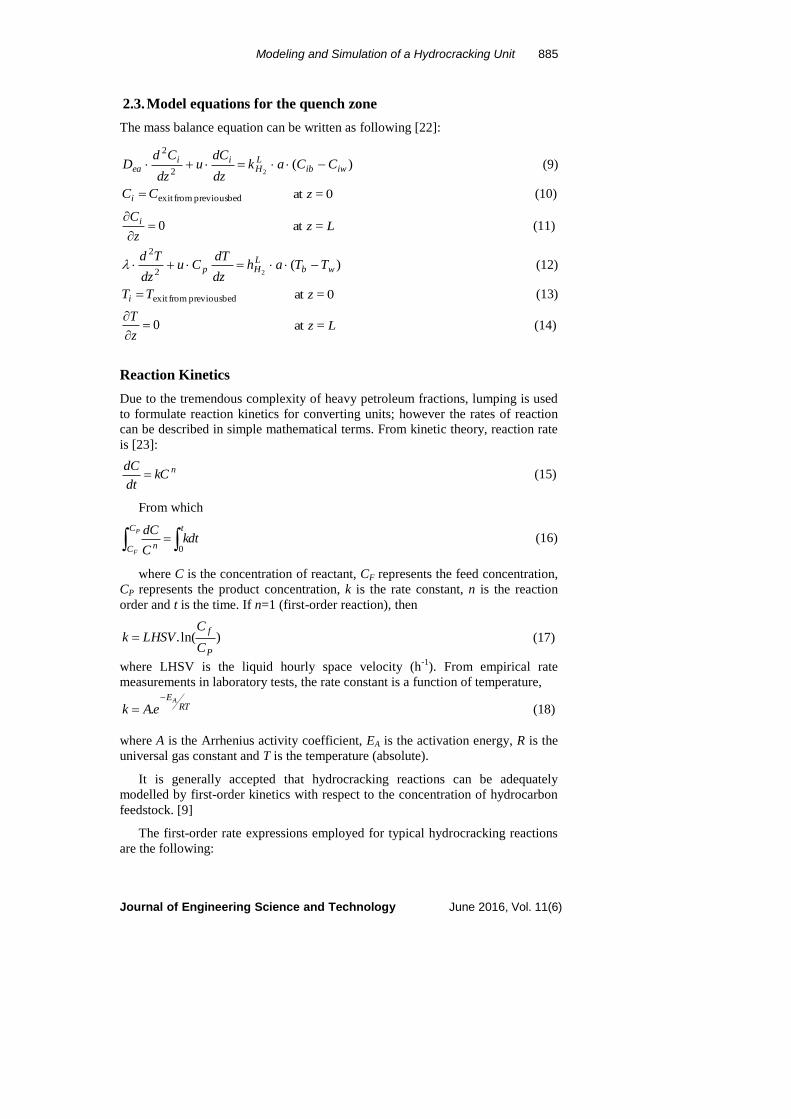
3.3. Effect of wall heat transfer coefficient (hw) on temperature profile

Several correlations were studied such as Wijngaarden and Westerterp [28],

Borman et al. [28], Dixon and Cresswell [26], Tobis and Ziolkowski [29], Hahn

and Achenbach [29]; to evaluate the wall heat transfer coefficient, and it was

found that all of them gave the same good results in the axial direction as shown

420

425430

435440

445450455460

0 2 4

Tem

pe

ratu

re ◦

C

Length m

Temperatureprofile usingDwmirel et al.

Temperatureprofile usingBrunell et al

Measuredtemperature

420

425

430

435

440

445

0 1 2 3

Tem

pe

ratu

re ◦

C

Radius m

Measuredtemperature

Dwmirel et al.

Brunell et al



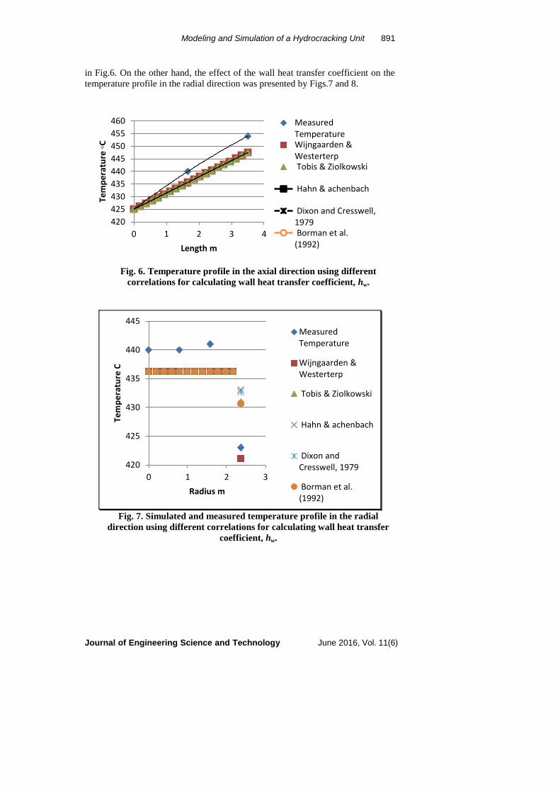
in Fig.6. On the other hand, the effect of the wall heat transfer coefficient on the

temperature profile in the radial direction was presented by Figs.7 and 8.

Fig. 6. Temperature profile in the axial direction using different

correlations for calculating wall heat transfer coefficient, hw.

Fig. 7. Simulated and measured temperature profile in the radial

direction using different correlations for calculating wall heat transfer

coefficient, hw.

420

425

430

435

440

445

450

455

460

0 1 2 3 4

Tem

pe

ratu

re ◦

C

Length m

MeasuredTemperatureWijngaarden &Westerterp Tobis & Ziolkowski

Hahn & achenbach

Dixon and Cresswell,1979 Borman et al.(1992)

420

425

430

435

440

445

0 1 2 3

Tem

pe

ratu

re C

Radius m

MeasuredTemperature

Wijngaarden &Westerterp

Tobis & Ziolkowski

Hahn & achenbach

Dixon andCresswell, 1979

Borman et al.(1992)



Fig. 8. Simulated temperature profile in the radial direction using

Wijngaarden and Westerterp correlation.

As shown from the previous figures, the relationship of Wijngaarden and

Westerterp [28] shown in table 5, gave the closest temperature profile in the radial

direction as it gave the lowest value of the wall heat transfer coefficient which

results in a low rate of heat transferred so low wall temperature value and vice

versa.

Table 5. Experimental correlations for the wall heat transfer coefficient

Authors wall heat transfer coefficient Experimental

conditions

Wijngaarden

and

Westerterp[28]

4.0, Nu9.2Bi ppw

-

Borman et al.

[28]

41.0Re29.2Nu pw

valid for 150 <

Rep < 2000

Dixon and

Cresswell[28]

25.0, Re0.3)/(Bi ptppw Rd

valid for Rep > 40

Tobis and

Ziolkowski[29]

33.08.01, Pr)]1[Re/(/18.0 pffw D

-

Hahn and

Achenbach[30] 3/161.0 PrRe)

/

11(Nu

dDw

valid for 50 < Rep

< 2 x 104

Fig. 8 shows the simulated temperature profile in the radial using

Wijngaarden and Westerterp correlation. As shown from the previous figures that

both the conversion and temperature profiles in the radial direction do not have

high deviation.

0 0.5 1 1.5 2 2.5420

422

424

426

428

430

432

434

436

438Temperature profile at the middel of the bed

Radius m

Tem

pera

ture

C



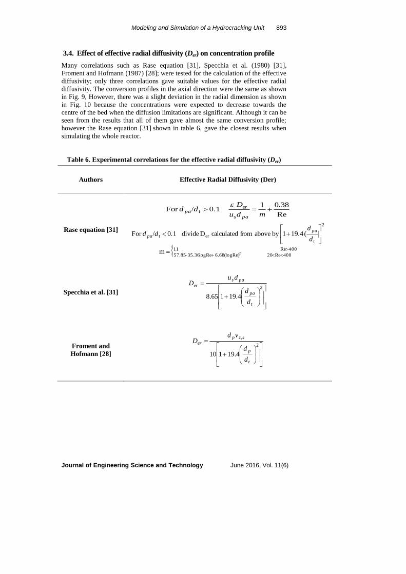
3.4. Effect of effective radial diffusivity (Der) on concentration profile

Many correlations such as Rase equation [31], Specchia et al. (1980) [31],

Froment and Hofmann (1987) [28]; were tested for the calculation of the effective

diffusivity; only three correlations gave suitable values for the effective radial

diffusivity. The conversion profiles in the axial direction were the same as shown

in Fig. 9, However, there was a slight deviation in the radial dimension as shown

in Fig. 10 because the concentrations were expected to decrease towards the

centre of the bed when the diffusion limitations are significant. Although it can be

seen from the results that all of them gave almost the same conversion profile;

however the Rase equation [31] shown in table 6, gave the closest results when

simulating the whole reactor.

Table 6. Experimental correlations for the effective radial diffusivity (Der)

Authors Effective Radial Diffusivity (Der)

Rase equation [31]

Re

38.01 0.1 /For

s

ert

mdu

Ddd

papa

2

tert ( 19.41by above from calculated D divide 0.1 /For

d

ddd

pa

pa

400Re 11

400Re20 (logRe) 6.68 logRe 35.36 - 57.85 2m

Specchia et al. [31]

2

4.19165.8t

pa

pas

er

d

d

duD

Froment and

Hofmann [28]

2

,

4.19110t

p

szp

er

d

d

vdD



Fig. 9. Simulated percentage conversion in the axial dimension using

different correlations for effective radial diffusivity.

Fig. 10. Simulated percentage conversion in the radial dimension using

different correlations for effective radial diffusivity.

3.5. Effect of cooling medium (quench zone) on conversion

Figs. 11 and 12 show the effect of quench zone on conversion for the first reactor

and the second reactor respectively. As shown from the figures, the conversion

increases slightly in the quench zone for both reactors despite the absence of a

catalyst. The results can be explained by two points: Hydrogen addition in this

part of the reactor may lead to increase the reaction rate that increases the

conversion. The main aim of the quench zone is to reduce the temperature and

because the reaction is exothermic conversion at equilibrium is higher.

0

2

4

6

8

10

12

14

16

18

20

0 1 2 3 4

% c

on

vers

ion

Length m

Conversion profileusing Rase, H. F.

Conversion profileusing Specchia etal.

Conversion profileusing Froment andHofmann

8.404

8.406

8.408

8.41

8.412

8.414

8.416

8.418

8.42

8.422

8.424

8.426

0 1 2 3

% C

on

vers

ion

Radius m

Conversion profileusing Rase, H. F.

Conversion profileusing Specchia etal.

Conversion profileusing Froment andHofmann



Fig. 11. Actual and simulated percentage conversion for quench zone in

the radial dimension for first reactor.

Fig. 12. Actual and simulated percentage conversion for quench zone in

the radial dimension for second reactor.

4. Conclusions

A rigorous two-dimensional model, including conservation equations of mass and

energy was developed for simulating the operation of a hydrocracking Unit. Both

the catalyst bed and quench zone have been included in this integrated model. The

model is capable of predicting temperature and concentration profiles inside

hydrocracking unit in both radial and axial directions. Simulation results have

0

10

20

30

40

50

60

70

80

0 50 100 150

%C

on

vers

ion

% of the reactor height

Calculated %conversion

Measured %conversion

quench zone 1

quench zone 2

0

10

20

30

40

50

60

70

80

0 20 40 60 80% of the reactor height

Calculated %conversion

Measured %conversion



been tested against available data from an actual plant. A comparison between the

calculated and available data shows that this two dimensional model can represent

the unit actual data very well. The following conclusions have been withdrawn:

For concentration profiles, the percentage deviation in the first reactor was

found to be 9.28% and 9.6% for the second reactor.

A Maximum deviation of 2.4% was found in temperature profiles.

In the quench zone the percent deviation in temperature was found to be 0.76%.

Wakao et al. Correlation shown in Table 3, for evaluating Pellet heat Transfer

Coefficient (hp) predicts the reactor temperature profile with a higher

accuracy than Handley and Heggs Correlation.

Correlations of Brunell et al. and Dwmirel et al. shown in Table 4. gave a

suitable value for the effective thermal conductivity.

Correlation of Wijngaarden and Westerterp shown in Table 5, for evaluating

the wall heat transfer coefficient gave the closest temperature profile in the

radial direction as it gave the lowest value of the wall heat transfer coefficient

which results in low temperature value.

Rase equation shown in Table 6, for the calculation of the effective

diffusivity gave the closest results when considering the whole reactor.

References

1. Kumar, A.; and Sinha, S. ( 2012). Steady state modelling and simulation of

hydrocracking reactor. Petroleum & Coal, 54(1); 59-64.

2. Parkash,S.(2003). Refining process handbook. USA, Elsevier.

3. Hsu, C.S.; and Robinson P.R. (2006). Practical advances in petroleum

processing. Volume 1, USA, Springer Science.

4. Canan, Ü.and Arkun, Y. (2012). Steady-state modelling of an industrial

hydrocracking reactor by discrete lumping approach. Proceedings of the

World Congress on Engineering and Computer Science, San Francisco, USA.

5. Meyers, R.A. (1996), Handbook of petroleum processes, New York,

McGraw-Hill.

6. Bahmani,M.; Mohadecy,R.S.; and Sadighi S. (2009). Pilot plant and

modeling study of hydrocracking, hydrodenitrogenation and

hydrodesulphurization of vacuum gas oil in a trickle bed reactor. Petroleum

& Coal, 51 (1), 59-69.

7. Ancheyta-Juaârez, J.; Loâpez-Isunzac, F.; and Aguilar-Rodrõâguez, E.

(1999). 5-Lump kinetic model for gas oil catalytic cracking. Applied

Catalysis A: General, 177, 227-235.

8. Sadighi,S.; Ahmady,A. ; and Mohaddecy, R. S. (2010). 6-Lump kinetic

model for a commercial .vacuum gas oil hydrocracker. International Journal

Of Chemical Reactor Engineering, Volume 8.

9. Ancheyta,J.; Sánchez,S.; and Rodrguez,M.A. (2005). Kinetic modeling of

hydrocracking of heavy oil fractions: a review. Catalysis Today, 109, 76 –92.



10. Bahmani, M.; Sadighi, S.; Mashayekhi, M. Mohaddecy, S.R.S.; and Vakili,

D. (2007). Maximizing naphtha and diesel yields of an Industrial

hydrocracking unit with minimal Changes. Petroleum & Coal, 49(1), 16-20.

11. Bhutani, N.; Ray, A. K.; and Rangaiah, G. P. (2006). Modeling, simulation,

and multi-objective optimization of an industrial Hydrocracking unit.

Industrial Engineering Chemical Research, 45, 1354 -1372.

12. Elizalde, I.; Rodríguez, M. A.; and Ancheyta, J. (2010). Modeling the effect

of pressure and temperature on the hydrocracking of heavy crude oil by the

continuous kinetic lumping approach. Applied Catalysis A: General, 382,

205 –212.

13. Alvarez, A.; Ancheyta, J.; and Muñoz, J.A.D. (2009). Modeling, simulation

and analysis of heavy oil hydroprocessing in fixed-bed Reactors employing

liquid quench streams. Applied Catalysis A: General, 361, 1–12.

14. Alvarez, A.; and Ancheyta, J. (2008). Modeling residue hydroprocessing in a

multi-fixed-bed reactor system. Applied Catalysis A: General, 351, 148–158.

15. Verstraete, J.J.; Le Lannic, K. ; And Guibard I. (2007). Modeling fixed-bed

residue hydrotreating processes. Chemical engineering science, 62, 5402 –

5408.

16. Aubé, F., and Sapoundjiev, H. (2000). Mathematical model and numerical

simulations of catalytic flow reversal reactors for industrial applications.

Computers and chemical engineering, 24, 2623–2632.

17. Béttega, R.; Moreira, M. F. P.; Corrêa, R. G. Freire, J. T. (2011).

Mathematical simulation of radial heat transfer in packed beds by

Pseudohomogeneous modeling. Particuology, 9, 107 –113.

18. Jung-Hwan, P. (1995). Modeling of transient heterogeneous two-dimensional

catalytic packed bed reactor. Korean Journal of Chemical Engineering,

12(1), 80-87.

19. Houcque, D. (2005). Introduction to matlab for engineering students.

20. Moustafa, T. M.; Abou-Elreesh, M.; and Fateen, S. K. (2007). Modeling,

simulation, and optimization of the catalytic reactor for methanol oxidative

dehydrogenation, Excerpt from the Proceedings of the COMSOL Conference,

Boston,USA.

21. Grevskott, S.; Rusten, T.; Hillestad, M.; Edwin, E.;and Olsvik, O. (2001).

Modeling and simulation of a steam reforming tube with furnace, Chemical

Engineering Science, 56, 597-603.

22. Fogler, H.S. (2006). Elements of chemical reaction engineering (4th

ed.).

USA, Pearson Education, Inc.

23. Giavarini, C.;and Trifirò, F. (2006).Encyclopaedia of hydrocarbons: refining

and petrochemicals .vol (2) , Italy, Marchesi Grafiche Editoriali S.P.A.

24. Jarullah, A. T.; Mujtaba, I.M.; and Wood, A.S. (2011). Kinetic parameter

estimation and simulation of trickle-bed reactor for hydrodesulfurization of

crude oil. Chemical Engineering Science, 66, 859–871.

25. Ghaj J. (2005). Non-boiling heat transfer in gas- liquid flow in pipes. Journal of

the Brazilian Society of Mechanical Science & Engineering, Vol. XXVII, 1.

26. Nield‏, D.A.; and Bejan, A.(2013)‏. Convection in porous media. (4th

ed.). New

York.



27. Wen, D.; and Ding,Y. (2006). Heat transfer of gas flow through a packed

bed, Chemical Engineering Science, 61, 3532 - 3542.

28. Wesenberg, M.H. (2006). Gas heated steam reformer modeling. Ph.D thesis,

13-57.

29. Legawlec, B. ; and Ziolkowski, D.( 1995). Mathematical simulation of heat

transfer withen tubler flow apperatus with packed bed by a model

considering system inhomogenity. Chemical Engineering Science, Vol. 50, 4,

673- 683.

30. Achenbach, E. (1994). Heat and flow characteristics of packed beds. Institute

of energy process engineering, Germany.

31. Iordanidis, A.A. (2002). Mathematical modeling of catalytic fixed bed

reactors. Ph.D Thesis, 19-54.

Date post:	04-Apr-2018
Category:	Documents
Upload:	hakhue
View:	226 times
Download:	5 times

MODELING AND SIMULATION OF A HYDROCRACKING UNITjestec.taylors.edu.my/Vol 11 issue 6 June...

Documents