79
Modeling and Simulation of a Small- Scale Polygeneration Energy System Dimosthenis Chitas (Concerto Programme, 2015a)

Modeling and Simulation of a Small-
Scale Polygeneration Energy System
Dimosthenis Chitas
(Concerto Programme, 2015a)

-2-
Master of Science Thesis EGI 2015: MJ211X
Modeling and Simulation of a Small-Scale
Polygeneration Energy System
Dimosthenis Chitas
Approved
2015/10/21
Examiner
Dr. Anders Malmquist
Supervisor
Sara Ghaem Sigarchian
Commissioner
Contact person
Abstract
The polygeneration is an innovative and sustainable solution which has become an attractive concept.
The simultaneous production of electricity, heating and cooling including hot and cold water
respectively in autonomous smaller energy systems can manage a more flexible and environmentally
friendly system. Furthermore distributed generation and micro scale polygeneration systems can
perform the increase of the utilized renewable energy sources in the power generation. The
aforementioned energy systems can consist of several power generation units however the low emission
levels, the low investment costs and the fuel flexibility of microturbines are some of the reasons that the
study of the microturbines in polygeneration systems is a crucial necessity.
In this study, an autonomous small-scale polygeneration energy system is investigated and each
component is analyzed. The components of the system are a microturbine, a heat recovery boiler, a heat
storage system and an absorption chiller. The purpose of this work is the development of a dynamic
model in Matlab/Simulink and the simulation of this system, aiming to define the reliability of the
model and understand better the behavior of such a system. Special focus is given to the model of the
microturbine due to the complexity and the control methods of this system. The dynamic model is
mainly based on thermodynamic equations and the control systems of the microturbine on previous
research works. The system has as a first priority the electricity supply while thermal load is supplied
depending on the electric demand. The thermal load is supplied by hot water due to the heat recovery
which takes place at the heat recovery boiler from the flue gases of the microturbine. Additionally the
design of the system is investigated and an operational strategy is defined in order to ensure the efficient
operation of the system. For this reason, after creating the load curves for a specific load, two different
cases are simulated and a discussion is done about the simulation results and the future work.

-3-

-4-
Examenasarbete EGI 2015: MJ211X
Modelering och simulering av ett småskaligt
polygeneration energisystem
Dimosthenis Chitas
Approved
2015/10/21
Examiner
Dr. Anders Malmquist
Supervisor
Sara Ghaem Sigarchian
Commissioner
Contact person
Sammanfattning
Polygeneration är en innovativ och hållbar lösning som har blivit ett attraktivt koncept. Den samtida
produktionen av el, värme och kyla (inkl. varmt och kallt vatten) i autonoma mindre energisystem kan leda
till ett mer flexibelt och miljövänligare system. Dessutom kan distribuerade energi- och småskaliga
polygenerationsystem leda till större användning av förnybara energikällor i kraftproduktion. De tidigare
nämda energisystemen kan bestå av många kraftproduducerande enheter, bland annat mikroturbiner. De
låga utsläppen, det låga investeringspriset samt bränsleflexibiliteten av mikroturbiner är några av
fördelarna till att undersökningen av mikroturbiner i polygenerationsystem är en viktig nödvändighet. I
den här undersökningen analyseras och undersöks varje komponent i ett autonomiskt småskaligt
energisystem. Systemets komponenter är en mikroturbin, en värmeväxlare, ett värmelagringssystem och
ett absorptionskylsystem. Målet med den här undersökningen är att utveckla en dynamisk modell för att
definiera pålitligheten av modellen, simulera systemet med hjälp av Matlab/Simulink och få en bättre
förståelse av systemets beteende. Särskilt fokus ges på mikroturbinens model på grund av systemets
komplexitet och kontrollmetoderna. Den dynamiska modellen är främst baserad på termodynamiska
ekvationer och kontrollsystemen av mikroturbinen är baserade på tidigare examensarbeten. Systemets
första prioritet är elförsörjningen så mängden av spillvärme beror på den elektriska förbrukningen. Den
termiska belastningen, består av värme och kylning, den levereras av varmvatten som värms upp genom
spillvärmen från mikroturbinen. Dessutom undersöks systemets design och en operativ strategi fastställs
för att garantera en genomförbar systemoperation. Av denna anledning så utvecklades två olika scenarion
av belastningskurvor, dessa simulerades och därefter diskuterades resultaten och framtida arbeten.

-5-
Acknowledgement
I would like to show my gratitude to my supervisor, Sara Ghaem Sigarchian, for giving me the opportunity
to work with this Master Thesis and her supervision although the difficulties due to the distance.
Furthermore I would like to thank Dr. Anders Malmquist for his useful advices and his contribution to
the modeling part of this work. Moreover thanks to “InnoEnergy” and to the “project STandUP for
Energy” for enabling a research environment that has been a necessary prerequisite for carrying out this
work. I would also like to thank Stamatia Gkiala and Moksadur Rahman for their help and assistance
during these six months.
Last but not least I would like to thank my family for supporting me spiritually throughout writing this
thesis and my life in general.
Dimosthenis Chitas
Stockholm, September 2015
-6-
Tables of Contents
1 Introduction ........................................................................................................................................................14
1.1 Goals and objectives .................................................................................................................................14
2 Methodology .......................................................................................................................................................16
2.1 System boundaries ....................................................................................................................................16
2.2 Limitations .................................................................................................................................................16
2.3 Literature survey ........................................................................................................................................16
2.4 Research approach ....................................................................................................................................16
2.5 Results and discussion ..............................................................................................................................17
3 Sustainability and power generation systems .................................................................................................18
3.1 Distributed energy generation and small Scale polygeneration energy systems – Background
studies ......................................................................................................................................................................19
3.2 Existing polygeneration systems .............................................................................................................21
3.2.1 Polycity project .................................................................................................................................21
3.2.2 Other existing polygeneration systems .........................................................................................23
4 Design of a polygeneration system ..................................................................................................................25
4.1 Description of the system ........................................................................................................................26
4.1.1 Microturbine .....................................................................................................................................26
4.1.2 Heat Storage ......................................................................................................................................30
4.1.3 Absorption chiller ............................................................................................................................32
5 Modeling and control of a polygeneration system ........................................................................................34
5.1 Data analysis and mathematical equations ............................................................................................34
5.2 System modeling .......................................................................................................................................40
5.2.1 Microturbine model .........................................................................................................................41
5.2.2 Heat Recovery ..................................................................................................................................44
5.2.3 Permanent magnet synchronous generator .................................................................................45
5.2.4 Heat Storage ......................................................................................................................................45
5.2.5 Absorption Chiller ...........................................................................................................................46
5.3 Model validation ........................................................................................................................................46
6 The case study .....................................................................................................................................................49
6.1 Electric, heating and cooling demand ....................................................................................................49
6.2 Simulation results ......................................................................................................................................53
6.2.1 January ...............................................................................................................................................53
6.2.2 August ................................................................................................................................................58
7 Conclusions and future work ...........................................................................................................................64
Bibliography .................................................................................................................................................................66
Appendix I – Data analysis ........................................................................................................................................70

-7-
Assumptions ............................................................................................................................................................70
Calculations .............................................................................................................................................................70
Specific fuel consumption .................................................................................................................................70
Gas content .........................................................................................................................................................71
Tank capacity selection ......................................................................................................................................71
Heat exchanger effectiveness ...........................................................................................................................71
System efficiencies..............................................................................................................................................71
Appendix II – System modeling ...............................................................................................................................72
Appendix III – Case study .........................................................................................................................................79

-8-
Table of Figures
Figure 1. Polygeneration System ...............................................................................................................................15
Figure 2. Projection from IEA for the worldwide electricity generation by 2035 (Chu &Majumdar, 2012).
........................................................................................................................................................................................18
Figure 3. A polygeneration energy system (Concerto Programme, 2015a). .......................................................20
Figure 4. Polycity project in Barcelona (Concerto Programme, 2015a). ............................................................21
Figure 5. Cogeneration system and absorption chiller (Concerto Programme, 2015c) ...................................22
Figure 6. I-CEMS concept(Concerto Programme, 2015c). ..................................................................................22
Figure 7. Polycity project in Ostfildern, Germany (Concerto Programme, 2015d). ........................................23
Figure 8. Polygeneration concept. ............................................................................................................................25
Figure 9. Flow chart of the polygeneration system. ...............................................................................................26
Figure 10. Folded primary surface of recuperators (Soares, 2007). .....................................................................27
Figure 11. Recuperated cycle of a microturbine and a T-S diagram (Stine & Geyer, 2001)............................27
Figure 12. Schematic presentation of a microturbine (Mansouri, Nikpey, &Assadi, 2014). ...........................28
Figure 13. Main components for Turbec T-100 PH (Turbec, 2009). .................................................................29
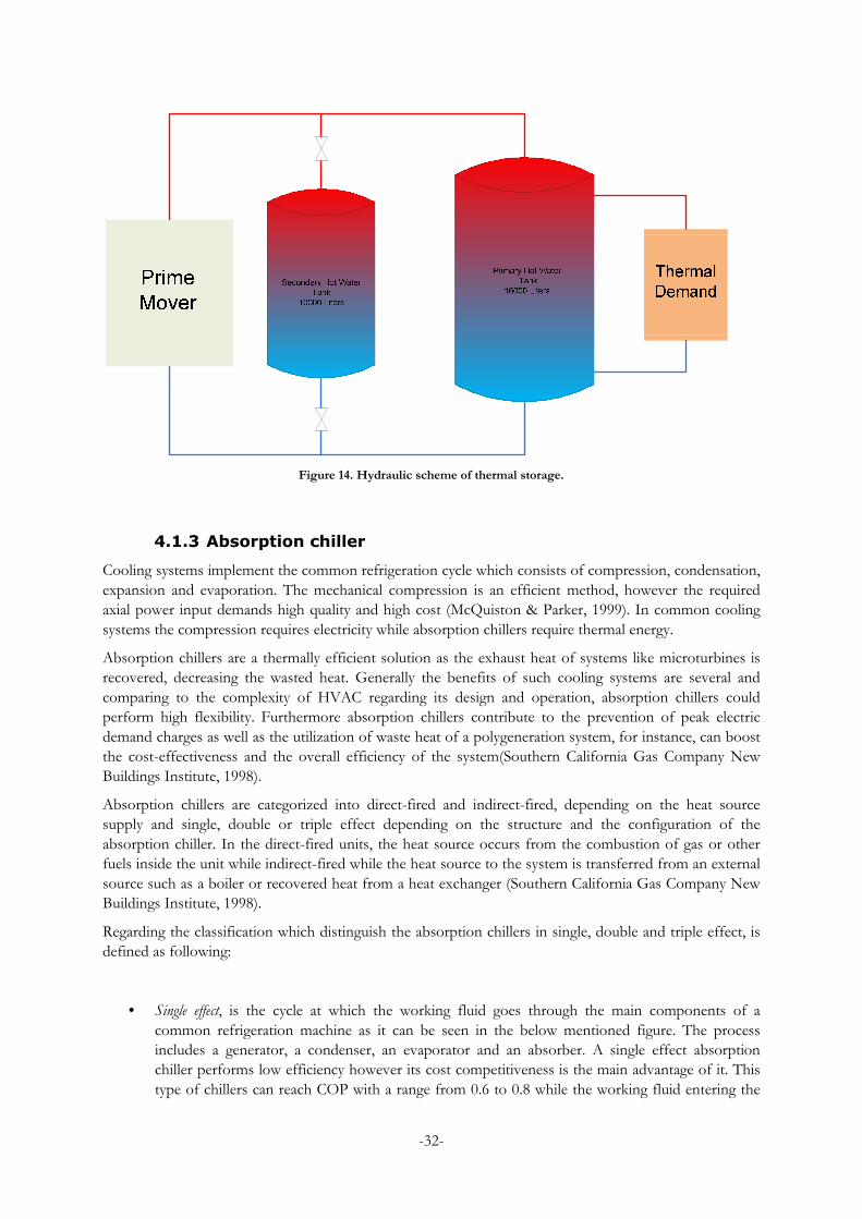
Figure 14. Hydraulic scheme of thermal storage. ...................................................................................................32
Figure 15. Single-effect absorption refrigeration cycle (Southern California Gas Company New Buildings
Institute, 1998). ............................................................................................................................................................33
Figure 16. Gas turbine cycle (Mansouri, Nikpey, &Assadi, 2014) .......................................................................34
Figure 17. Electrical efficiency for different electrical loads (Camporeale et al., 2014). ..................................35
Figure 18. Data extraction with WebPlotDigitizer(Rohatgi, 2015). ....................................................................35
Figure 19. Pressure ratio for different air mass flow rates (Camporeale et al., 2014). ......................................37
Figure 20. Isentropic efficiency of the compressor for different air mass flow rates (Camporeale et al.,
2014). .............................................................................................................................................................................37
Figure 21. Microturbine block diagram. ..................................................................................................................41
Figure 22. Turbine block. ...........................................................................................................................................42
Figure 23. Speed control system. ..............................................................................................................................43
Figure 24. Temperature control system. ..................................................................................................................43
Figure 25. Fuel system control. .................................................................................................................................44
Figure 26. Heat storage, auxiliary system and controlling valves. ........................................................................46
Figure 27. Thermal load due to the cooling demand, provided by the absorption chiller. .............................46
Figure 28. Points specification for validation test run. ..........................................................................................47
Figure 29. Modeling results of the electric efficiency compared with data and error factors. ........................47
Figure 30. Normalized curve of hourly electric load in (a) winter, (b) summer. ...............................................49
Figure 31. Average load curve of residential air conditioning systems in Italy and Greece, 2000
(Kärkkäinen, 2011). .....................................................................................................................................................50
Figure 32. Normalized cooling demand (data taken from (Kärkkäinen, 2011)) ...............................................50
Figure 33. Normalized heating demand (Bianchi et al., 2014). ............................................................................51
Figure 34. Hourly electric demand per day, January. .............................................................................................51
Figure 35. Hourly electric demand per day, August. .............................................................................................52
Figure 36. Hourly heating demand per day in January. .........................................................................................52
Figure 37. Hourly cooling demand per day in August. .........................................................................................53
Figure 38. Consumed mechanical power of compressor, produced mechanical power of turbine and
generated electricity by the generator. ......................................................................................................................54
Figure 39. Air and gas flow rates in the microturbine for different loads. .........................................................54
Figure 40. Compressor inlet (T1), compressor outlet (T2) and recuperator inlet (T3) temperature. ............55
Figure 41. Turbine inlet (T4), turbine outlet (T5) and recuperator outlet (T6) temperature. .........................56
Figure 42. Heat exchanger temperatures at the gas and water stream. ...............................................................56
Figure 43. Water temperatures in the tanks, before the heat exchanger and after the heat exchanger. ........57
Figure 44. Recovered heat by the heat exchanger and additional supplied het by the auxiliary boiler. .........58

-9-
Figure 45. Consumed mechanical power of compressor, produced mechanical power of turbine and
generated electricity by the generator. ......................................................................................................................59
Figure 46. Air and gas flow rates in the microturbine for different loads. .........................................................59
Figure 47. Compressor inlet (T1), compressor outlet (T2) and recuperator inlet (T3) temperature. ............60
Figure 48. Turbine inlet (T4), turbine outlet (T5) and recuperator outlet (T6) temperature. .........................61
Figure 49. Heat exchanger temperatures at the gas and water side. ....................................................................61
Figure 50. Water temperatures in the tanks, before the heat exchanger and after the heat exchanger. ........62
Figure 51. Recovered heat by the heat exchanger and additional supplied het by the auxiliary boiler. .........63
Figure 52. Load, generator and microturbine .........................................................................................................73
Figure 53. Heat exchanger and heat storage ...........................................................................................................74
Figure 54. Mictoturbine ..............................................................................................................................................75
Figure 55. Heat exchanger. ........................................................................................................................................76
Figure 56. Primary tank ..............................................................................................................................................77
Figure 57. Secondary tank. .........................................................................................................................................78
Table of Tables
Table 1. Performance characteristics of Turbec T-100 (Turbec, 2009). .............................................................29
Table 2. Air, fuel and gas flow rates. ........................................................................................................................36
Table 3. Compressor pressure ratio and isentropic efficiency. ............................................................................37
Table 4. Gas turbine system efficiencies. .................................................................................................................71
Table 5. Model input parameters. .............................................................................................................................72
Symbols
LHVNG Lower Heating Value [kJ/kg K]
cosφ Power factor [-]
Cpair Specific heat of air [kJ/kg K]
Cpgas Specific heat of gas [kJ/kg K]
Cpw Specific heat of water [kJ/kg K]
f Stoichiometric air-to-fuel ratio [-]
IL Line current [A]
LHV Lower Heating Value [kJ/kg K]
mair Air mass flow rate [kg/s]
mf Fuel mass flow rate [kg/s]
mg Gas mass flow rate [kg/s]
mw Water mass flow rate [kg/s]
N Rotational speed [RPM]
Np.u. Rotational speed [pu]
P Pressure [Pa]
PC Compressor power [kW]

-10-
Pel Electric power [kW]
PGT Gas turbine power [kW]
PR Pressure ratio
PT Turbine power [kW]
Qfuel Input thermal heat [kW]
Qrec Recovered heat [kW]
RH Relative humidity [%]
T1 Inlet compressor temperature [K]
T2 Outlet compressor temperature [K]
T3 Recuperator outlet temperature, air side [K]
T4 Turbine inlet temperature [K]
t5 Turbine outlet temperature [ C]
T5 Turbine outlet temperature [K]
T6 Recuperator outlet temperature, gas side [K]
T7 Exhaust temperature [K]
T8 Water temperature to storage [K]
TC Compressor torque [Nm]
Tm Shaft mechanical torque [Nm]
Ts Hot water to temperature to the heat exchanger [K]
TT Turbine torque [Nm]
Vph Phase voltage [V]
x Gas content [%]
xc Compressor pressure ratio coefficient [-]
Greek Symbols
β Specific fuel consumption
γc Specific heat ratio [-]
ηcomb Combustion efficiency [-]
ηel Electric efficiency [-]
ηis,c Isentropic compressor efficiency [-]
ηgen Generator efficiency [-]
ηm Mechanical efficiency of the turbine [-]
ε Effectiveness [-]
ω Rotational speed [rad/sec]

-11-
Symbols in the model
c Fuel system constant
C1 Governor lead time constant [s]
C2 Governor lag time constant [s]
C3 Radiation shield time constant [s]
C4 Thermocouple shield time constant [s]
C5 Temperature controller time constant [s]
COP Coefficient of performance
K Governor Gain
k_NL No load consumption factor
K4 Radiation constant
K5 Radiation constant
Kf Fuel system actuator gain
Kv Valve position gain
M Tank capacity [l]
ma Air mass flow rate [kg/s]
mf Fuel mass flow rate [kg/s]
mf,boil Auxiliary boiler's fuel flow rate [kg/s]
mg Gas mass flow rate [kg/s]
mw,HE Total water flow to the HE [kg/s]
mw1 Water flow from Tank 1 to the HE [kg/s]
mw2 Water flow from Tank 2 to the HE [kg/s]
mws1 Water flow rate to Tank 1 [kg/s]
mws2 Water flow rate to Tank 2 [kg/s]
N Speed [RPM]
n_is_c Isentropic compressor efficiency [-]
N_Ref Reference speed [RPM]
PC Compressor power [kW]
Pel Electric power [kW]
PR Pressure ratio
PT Turbine power [kW]
Qboiler Heat from the auxiliary boiler [kW]
Qextr Extracted heat from Tank 2 [kW]
Qload Thermal load [kW]
Qlosses Tank thermal losses [kW]
Qrec Recovered heat (kW]
SM Turbine smoothness coefficient
SM1 Turbine smoothness coefficient 1
T1 Ambient temperature [ C]
T2 Outlet compressor temperature [K]
-12-
T3 Recuperator outlet temperature, air side [K]
T4 Turbine inlet temperature [K]
T5 Turbine outlet temperature [K]
T6 Recuperator outlet temperature, gas side [K]
T7 Exhaust temperature [K]
T8 Water temperature to storage [ C]
TCD Compressor discharge time lag [s]
TCR Combustion reaction transport delay [s]
Tf Fuel system actuator time constant [s]
Ts,1 Water temperature in Tank 1 [ C]
Ts,2 Water temperature in Tank 2 [ C]
Ts,mix Water temperature before the HE [ C]
Tt Temperature controller integration constant [ C]
TTD Turbine exhaust transport delay [s]
Tv Valve position time constant [s]
xc Compressor pressure ratio coefficient [-]
z Speed control system constant
Abbreviations
A.C. Alternating Current
CHP Combined Heat and Power
CO2 Carbon Dioxide
COP Coefficient of performance
D.C. Direct Current
EC European Commissions
EER Energy Efficiency Ratio
EFmGT Externally Fired micro Gas Turbine
ESEER European Seasonal Energy Efficiency Ratio
EU European Union
GHG Greenhouse Gas Emissions
HVAC Heating Ventilation & Air Conditioning
I-CEMS Integrated Energy Management System
IEA International Energy Agency
ISO International Organization of Standardization
LHV Lower Heating Value
LVG Least Value Gate
MSW Municipal Solid waste
ORC Organic Rankine Cycle
PH Permanent Magnet Synchronous Generator
PID Proportional Integral Derivative
PMSG Power and Heat

-13-
PV Photovoltaic
RPM Revolutions per Minute
-14-
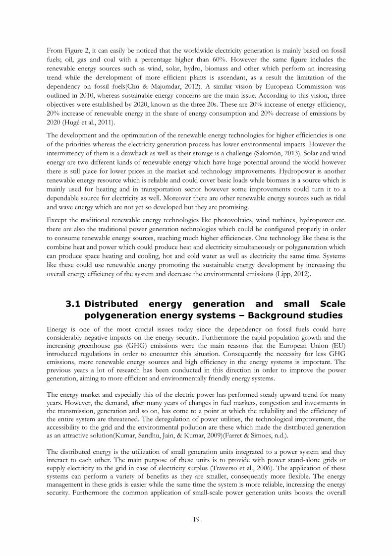
1 Introduction
According to Brundtland Commission, sustainability is defined as to meet the needs of the present
generation without compromising the ability of future generations to meet their needs (Salomón, 2013).
Today, many efforts are made, aiming to overcome challenges in the field of sustainability. Both the
population and economic growth have an impact on the energy consumption as well as the environment
is dramatically affected by the uninterrupted utilization of fossil fuels. For this reason, the nowadays
situation has set as a significant necessity for the investigation of more effective, sustainable and
environmentally friendly solutions in the field of energy production. The distributed energy is the
utilization of small generation units integrated to a power system which interact to each other. The main
purpose of these units is to provide with power stand-alone grids or supply electricity to the grid in case of
electricity surplus (Traverso, Massardo, & Scarpellini, 2006). The application of these systems can perform
a variety of benefits as they are smaller, consequently more flexible. The energy management in these grids
is easier while the same time the system is more reliable, increasing the energy security. Furthermore the
common application of small-scale power generation units boosts the overall energy efficiency as well as
the input energy can be based on renewable energy sources making the distributed generation a
sustainable solution (Farret & Simoes, n.d.). One type of distributed generation is the polygeneration
systems which can simultaneously produce space heating and cooling, hot and cold water as well as
electricity.
In this work a general discussion is included about the energy situation and sustainability as well as the
distributed generation and the polygeneration systems. More specifically advantages and disadvantages of
polygeneration systems are highlighted while the same time implemented or projected polygeneration
systems are presented. Furthermore special consideration is given to the microturbines and their
application as components of small-scale polygeneration systems. Consequently a small scale
polygeneration system is designed which consists of a microturbine, a heat storage, a heat recovery boiler
and absorption chiller. The main purpose is the modeling of this system in Matlab/Simulink in order to
understand better its behavior while special focus is given to the microturbine modeling due to its
complexity. The model is simulated for two different cases in which there is the maximum possible
heating demand in the first case and in the second case the maximum cooling demand.
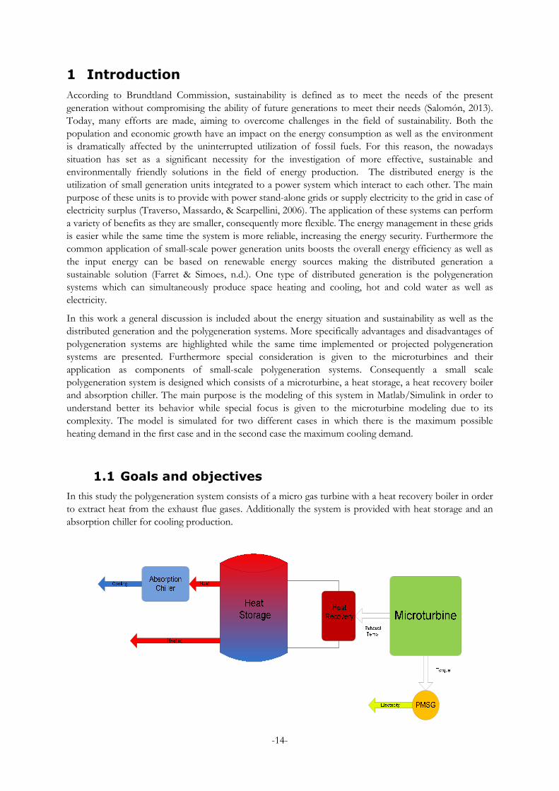
1.1 Goals and objectives
In this study the polygeneration system consists of a micro gas turbine with a heat recovery boiler in order
to extract heat from the exhaust flue gases. Additionally the system is provided with heat storage and an
absorption chiller for cooling production.

-15-
Figure 1. Polygeneration System
The investigation of the system is implemented by the development of a dynamic model in Simulink in
order to monitor the energy balance of the system and attempt to couple demand and production
accurately, making the entire system cost effective due to the minimization of the energy waste(Kallio,
2012).The research work includes the energy supply of a block of flats during two different days
throughout the year. Each of them is in different season of the year aiming to investigate the behavior of
the system under the maximum possible heating demand andunder the maximum possible cooling
demand.
The key factors of an efficient small-scale polygeneration system are the correct system sizing and configuration during the designprocess and control strategy as well as thepower management during the system operation. This thesis investigates how to achieve the above mentioned key factors with the aim to design an energy effective small-scale polygeneration system. Consequently the objectives of this thesis are to achieve:
� An optimal design The components of the system are already predetermined however the proper
configuration of the system considering the load is a crucial part of this work.
� A reliable model A model of a polygeneration system in Matlab/Simulink is expected to be created in order to monitor the energy balances and investigate the behaviour of this polygeneration system. This model should be validated and be as accurate as possible.
� An efficient and safeoperational strategy
An operational strategy should be defined aiming to ensure the smooth operation of the polygeneration system. The critical parameters of each component should be recognized and adjusted properly for an efficient and safe operational strategy.

-16-
2 Methodology
In this section the implemented research approach is analyzed. The research approach describes the main processes of a research work in order to complete it and achieve its objectives. These are the problem statement, the goals and objectives of this problem, the system boundaries, the literature review, the design process as well as the results and discussion. All of them except the goals and objectives which have already been mentioned are explained below as well as their main functions are described.
2.1 System boundaries
The system boundaries are confined to the energy input and output. The boundary starts at the required
energy to cover the load while it finishes at the available produced energy for the system. Furthermore
except the available energy, the auxiliary systems are taken into consideration in order to define the
amount of energy that should be produced by them in case the polygeneration system cannot cover the
whole demand throughout the year. Moreover this work investigates only the energy production and
demand whilst no economic facts are considered.
2.2 Limitations
The limitations should also be considered during the planning process of such a power system. The operation of a polygeneration system is based on three main factors; the users, the thermal storage and the electricity utility. Sometimes it is difficult to estimate the accurate energy demand and how it varies in time in order to match the energy production and demand effectively. The energy consumption depends on many different factors such as geographical position, type of user, lifestyle (if it is a residential user) and other local considerations (Ortiga, Bruno, Coronas, & Grossman, 2007). Furthermore another important factor is the thermal storage and its operation strategy that should be considered since it could affect the entire system which supplies a load with a dynamic behaviour (Ulloa, Míguez, Porteiro, Eguía, & Cacabelos, 2013). Last but not least as far as the components of the system are concerned regarding the data, their confidential character especially for those of the gas turbine is a fact that should be considered. This kind of data is hard to be found or to be provided by the manufacturer so the work is based on simulated results whereas the data were calculated by applying the basic thermodynamical equations.
2.3 Literature survey
The literature review is strongly interconnected to the system boundaries and the goals of the project. The
literature review starts with general information whereas it is similar to the structure of the report. The
literature study initially focused on information regarding the sustainability, the energy situation today and
the polygeneration systems. Furthermore a more intensive literature study was implemented regarding
each part of the system, their principle and characteristics. Afterwards, the process of the research
approach was continued with a study research regarding the modeling of each component, their
integration to the system in a sustainable and feasible way and how they can affect each other. Finally
information regarding the operational strategy and the control of systems like this is essential to be
determined.
2.4 Research approach
The research approach begins with the organization of the data since this is a crucial part of this work in
order to model the system and especially to model the gas turbine. The initial goal regarding this process
was experimental data to be found however due to the confidential character of this kind of data, it was

-17-
difficult to find them. Consequently this work is based on results of previous works whereas
thermodynamic calculations were implemented in order to estimate the data.
The next step of the research approach is the design process and the proper configuration of the system
components. This is one of the main processes of this work and it is the most crucial factor for the
objectives achievement and the final outcomes of the project. Τhe purpose of this process is to develop a
reliable dynamic model, including the system control. Afterwards the energy demand has to be considered
as well as both electrical and thermal load curves should be created and imported to the model. Finally the
model is simulated for two cases in order to study the behavior of the system under different situations.
2.5 Results and discussion
As far as the results are concerned, the model has firstly to be validated in order to define the variations of
the model in comparison with the experimental data and estimate any kind of possible variations between
the data and the simulation results. Afterwards the model runs for a whole day (24 hours) aiming to notice
the dynamic behaviour of the load throughout the day and how the system and its auxiliary equipment can
supply the load. The same process is repeated for two different days; winter and summer. The aim of the
both simulations is to investigate a day with only heating demand and a day with only cooling demand.
The final outcome of this research work is expected to be a reliable model which could be used as a tool
in the future in order to monitor the energy balance of a system, define an optimal sizing of the
installation and define an operational strategy, aiming to a more sustainable and feasible operation.
Moreover the results should be discussed and possible recommendations could be made regarding further
research in the future.

-18-
3 Sustainability and power generation systems
It is obvious that after the industrial revolution the world has become different. This was one of the main
reasons that the rapid technology improvement changed the humanity forever. Most of the daily common
processes have been substituted by others which are more efficient, easier and faster. Combustion engines
for electricity and transportation, steam powered ships and trains as well as the changes in the product
development are some examples. Afterwards this revolution was continued by the electrification of
buildings and other widely used technologies during the last century to come to nowadays habits. Today
modern space heating and cooling are playing an important role in the indoor comfort while the
transportation sector is also one of the main energy consumers (Chu & Majumdar, 2012). The daily life
became easier however that was the beginning of a dramatically energy consumption increase. The social
and technological development featured the importance of energy and the energy issues regarding
consumption, efficiency and emissions are becoming more and more, as the energy usage surpasses any
other historical data. For that reason energy isan issue which is always in the agenda as it has constituted
the key aspect of many crises directly or indirectly such as environmental pollution and geopolitical issues
respectively(Hugé, Waas, Eggermont, & Verbruggen, 2011).
Nowadays concerns regarding sustainability have been raised due to the population growth and the
environmental pollution. In one hand the population growth in combination with the economic and
prosperity growth have impact on the worldwide energy consumption, while on the other hand the
utilization of conventional fossil fuels contribute to the environmental pollution. Additionally the finite
character of the conventional energy resources is the main aspect of affecting the energy security, whereas
the energy price fluctuations are a common example. According to Brundtland, sustainability is defined as
to meet the needs of the present generation without compromising the ability of future generations to
meet their needs (Salomón, 2013). Consequently it had been undertaken the idea of sustainability to be
introduced to energy issues by researchers, policy makers and governments around the world, aiming to
establish a strategy which could maintain a feasible balance between energy security, environmental
protection and economic development.
In this direction the energy authorities are working on and the below mentioned figure by the
International Energy Agency (IEA) shows the energy mix today and the predicted situation with a
business as usual scenario and a new policies scenario by 2035.
Figure 2. Projection from IEA for the worldwide electricity generation by 2035 (Chu &Majumdar, 2012).
-19-
From Figure 2, it can easily be noticed that the worldwide electricity generation is mainly based on fossil
fuels; oil, gas and coal with a percentage higher than 60%. However the same figure includes the
renewable energy sources such as wind, solar, hydro, biomass and other which perform an increasing
trend while the development of more efficient plants is ascendant, as a result the limitation of the
dependency on fossil fuels(Chu & Majumdar, 2012). A similar vision by European Commission was
outlined in 2010, whereas sustainable energy concerns are the main issue. According to this vision, three
objectives were established by 2020, known as the three 20s. These are 20% increase of energy efficiency,
20% increase of renewable energy in the share of energy consumption and 20% decrease of emissions by
2020 (Hugé et al., 2011).
The development and the optimization of the renewable energy technologies for higher efficiencies is one
of the priorities whereas the electricity generation process has lower environmental impacts. However the
intermittency of them is a drawback as well as their storage is a challenge (Salomón, 2013). Solar and wind
energy are two different kinds of renewable energy which have huge potential around the world however
there is still place for lower prices in the market and technology improvements. Hydropower is another
renewable energy resource which is reliable and could cover basic loads while biomass is a source which is
mainly used for heating and in transportation sector however some improvements could turn it to a
dependable source for electricity as well. Moreover there are other renewable energy sources such as tidal
and wave energy which are not yet so developed but they are promising.
Except the traditional renewable energy technologies like photovoltaics, wind turbines, hydropower etc.
there are also the traditional power generation technologies which could be configured properly in order
to consume renewable energy sources, reaching much higher efficiencies. One technology like these is the
combine heat and power which could produce heat and electricity simultaneously or polygeneration which
can produce space heating and cooling, hot and cold water as well as electricity the same time. Systems
like these could use renewable energy promoting the sustainable energy development by increasing the
overall energy efficiency of the system and decrease the environmental emissions (Lipp, 2012).
3.1 Distributed energy generation and small Scale
polygeneration energy systems – Background studies
Energy is one of the most crucial issues today since the dependency on fossil fuels could have considerably negative impacts on the energy security. Furthermore the rapid population growth and the increasing greenhouse gas (GHG) emissions were the main reasons that the European Union (EU) introduced regulations in order to encounter this situation. Consequently the necessity for less GHG emissions, more renewable energy sources and high efficiency in the energy systems is important. The previous years a lot of research has been conducted in this direction in order to improve the power generation, aiming to more efficient and environmentally friendly energy systems. The energy market and especially this of the electric power has performed steady upward trend for many years. However, the demand, after many years of changes in fuel markets, congestion and investments in the transmission, generation and so on, has come to a point at which the reliability and the efficiency of the entire system are threatened. The deregulation of power utilities, the technological improvement, the accessibility to the grid and the environmental pollution are these which made the distributed generation as an attractive solution(Kumar, Sandhu, Jain, & Kumar, 2009)(Farret & Simoes, n.d.). The distributed energy is the utilization of small generation units integrated to a power system and they interact to each other. The main purpose of these units is to provide with power stand-alone grids or supply electricity to the grid in case of electricity surplus (Traverso et al., 2006). The application of these systems can perform a variety of benefits as they are smaller, consequently more flexible. The energy management in these grids is easier while the same time the system is more reliable, increasing the energy security. Furthermore the common application of small-scale power generation units boosts the overall

-20-
energy efficiency as well as the input energy can be based on renewable energy sources making the distributed generation a sustainable solution (Farret & Simoes, n.d.). As it is mentioned above regarding power generation systems which could promote the distributed generation, one of these is the combined heat and power generation (CHP) systems. CHP systems are energy systems which produce simultaneously heat and power. The main components of a CHP system are power generation units, a generator, a heat recovery system, a control system and an electric grid. The implementation of CHP systems has several advantages making this technology more attractive, since there is much lower wasted energy in comparison with other conventional energy systems. One step forward is the integration of cooling production applications to a CHP system can boost the overall efficiency of the application, producing space cooling and heating including hot and cold water as well as electricity. These systems are called polygeneration energy systems.
Nowadays small scale polygeneration systems are considered as an attractive solution due to their high energy efficiency and environmentally friendly character (Kumar et al., 2009). Small scale polygeneration systems have usually capacity up to 5 MW and supply the heating, electricity and cooling demand of a small area, a residential building or a commercial enterprise Elsied et al., 2014)(Kumar et al., 2009). They usually consist of one or more power generation units which are called prime movers such as micro-gas turbines, diesel engine generator sets, Stirling engines, fuel cells, solar PVs, wind turbines etc. Depending on the cycle of each energy system the prime movers produce directly electricity while exhaust heat is recovered from exhaust gases through a heat recovery boiler in order to provide heat in form of hot water to the heat storage system. Afterwards the heat storage system provides space heating or hot water as well as space cooling through an absorption chiller.
Figure 3. A polygeneration energy system (Concerto Programme, 2015a).
Moreover its multi-fuel capability depending on the system’s prime movers, allows to it to combine fossils fuels and renewable energy sources or even more substitute fossil with renewable sources, promoting the sustainability. Last but not least, the advantages of a small-scale polygeneration system compared to these of a large installation are of high significance. First of all the large power plants perform isolation losses due to the distance from the consumers having transmission losses. Additionally the isolation losses require high electricity demand as well as high heat losses can be performed due to the hot water distribution (Velez, 2010).

-21-
3.2 Existing polygeneration systems
The polygeneration is a concept which is getting more and more significant the last years since the
distributed energy systems and microgrids are environmentally friendly and more energy efficient
solutions. For this reason there are many projects around the world under planning and other already
under operation. Some of these projects have been presented are included in this section.
3.2.1 Polycity project
Concerto initiative is a European Commission funded initiative which supports the development of urban
areas in Italy, Spain and Germany aiming to introduce high shares of renewable energy in the primary
energy supply and optimize energy systems with higher energy efficiencies and more efficient buildings.
The project investigates three different cases/areas (Concerto Programme, 2015b).
• An area in Barcelona, Spain, which is underdeveloped with new buildings.
• An old district area in Turin, Italy, where renewals and renovations are conducted.
• And an area in a military area called Ostfildern, close to Stuttgart, Germany where there are both
new buildings and old existing buildings.
3.2.1.1 Polycity project in Barcelona, Spain
The Policity project in Barcelona is based on two factors; the efficient energy supply and the reduction of
the buildings’ energy demand. The polygeneration system consists of 4 cogeneration plants whereas the
majority of them consume natural gas and the electrical capacity is 47 MWe .The system also includes
biomass gasification with capacity of 1000 kg/h while solar energy is used for cooling purposes. Solar
climatization systems which combine thermal solar energy with thermal cooling equipment aim to cover
the cooling demand: space cooling and cold water. The solar collectors provide heat to the absorption
chillers with 600 kW thermal output and 700 MWh of cold water at 7 C.
Figure 4. Polycity project in Barcelona (Concerto Programme, 2015a).

-22-
3.2.1.2 Polycity project in Turin, Italy
Except the buildings refurbishment, in the area of Arquata in Turin, a special consideration was given to
the energy system of the area. The local electrical and heating demand are mainly supplied by a natural gas
cogenerator with capacity of 970 kWe and 1166 kWth while in case of peak demand the surpluses are
covered by three high efficiency boilers. Each household is equipped with a satellite control module
aiming to adjust the inlet flow valve of the hot water depending on the space heating thermostat while the
cooling demand in buildings is mainly provided by absorption chillers. Furthermore the capacity of the
solar power generation of Arquata’s energy system is one of the largest in Italy. Additionally photovoltaic
modules are installed on roof tops and balconies, reaching an annual production of 190 MWh (Concerto
Programme, 2015c).
Figure 5. Cogeneration system and absorption chiller (Concerto Programme, 2015c)
Consequently the combination of the buildings improvements in terms of heating losses and more
sustainable energy supply of the buildings with a polygeneration energy system, led to a sustainable,
efficient and environmentally friendly solution. The result was also contributed by the implementation of
the Integrated Energy Management System (I-CEMS).The purpose of this system is the coupling of
energy demand and supply with an intelligent control aiming to the optimization of the governance. The
principle of this operation can be seen in Figure 6 (Concerto Programme, 2015c).
Figure 6. I-CEMS concept(Concerto Programme, 2015c).
The above mentioned concept can perform energy savings, service quality, cost and emissions decrease.
The implementation of the aforementioned management system in combination with the applied energy
technologies resulted to 43% reduction of primary energy while the CO2 emissions decreased by 52%
(Concerto Programme, 2015c).

-23-
3.2.1.3 Polycity project Ostfildern, Germany
In an area close to Stuttgart, the city of Ostfildern, one of the Polycity project has been implemented
which includes 480 000 m2 of built area and an investment up to 1.5 billion euros. Ostfildern is an area
where there are either new or old buildings and they are provided by a 1MWel and 6.3 MWth organic
Rankine cycle (ORC) co-generation plant while most of the buildings are equipped with photovoltaics
with capacity of 70kW (Concerto Programme, 2015d).
Figure 7. Polycity project in Ostfildern, Germany (Concerto Programme, 2015d).
The ORC plant consumes wood chips while the entire energy system is equipped with two natural gas
boilers for peak periods. Only this plant is estimated that can provide 80% of heating demand and 50%
electrical demand of a 10 000 people population. Moreover the cooling demand of some buildings during
the warm months is produced by heat through a new technology lithium-bromide refrigerating machine,
being the first application implementing this kind of machine in Europe, while other buildings are
supplied by compression refrigerating machines (Concerto Programme, 2015d).
3.2.2 Other existing polygeneration systems
3.2.2.1 University Campus of Savona, Italy
The energy demand of the University campus of Savona in Italy is provided with energy by a
polygeneration system as well as decreasing the supplied electricity from the grid. The system is a high
level efficient energy system which utilizes renewable energy with electrical capacity 250 kWe and thermal
capacity 300kWth. The control of the system is executed by the Siemens Microgrid Manager aiming to
predict the energy demand and energy production by renewable energy sources. The entire project is
sponsored by Siemens (IEEE Spectrum, 2014).
3.2.2.2 Sydney Town Hall House trigeneration, Australia
The project begins in 2016 and contributes to the Sustainable Sydney 2030 project while it is expected to
reduce by 3% the carbon emissions of the city. The planned polygeneration system will supply the entire
building including the offices and it is estimated to reduce the energy consumption, resulting to the energy
cost reduction by $320 000 annually (City of Sydney, 2015).
3.2.2.3 Pulkovo Energy Center, Russia
The international airport of St. Petersburg planned a new terminal “Pulkovo-3” in 2013 with total area 94
thousand square meters. As far as its energy supply is concerned it is also based on the polygeneration

-24-
concept with 10 MW power while the cooling capacity of the system reaches 7 MW. The project is
considered as an innovative solution since it supplies this amount of cooling with energy efficiency ratio
(EER) equal to 7.67 at 100% load while its European seasonal energy efficiency ratio (ESEER) can
achieve the level of 8.78 at 100% load (Geoclima Smart HVAC Solutions, 2013).

-25-
4 Design of a polygeneration system
The design of a polygeneration system is based on a variety of processes however the first step is the
estimation of the energy demand in order to choose the appropriate prime movers and their capacity. The
energy demand depends on the geographical position and other local considerations as well as the kind of
the load is another crucial factor whereas it is usually difficult to define the user’s behavior (Ortiga et al.,
2007). Moreover after the energy demand prediction has been considered the appropriate system
configurations have to be made in order to analyze the behavior of the system. As it has already been
mentioned the configuration of the system and its components are predetermined, as the main focus of
this work is the microturbine. The implementation of small-scale generation units such as gas turbines in
polygeneration energy systems boosts the overall energy efficiency as well as far as the input energy can be
based on renewable energy sources making the distributed generation a sustainable solution (Farret &
Simoes, n.d.). One more reason that special consideration is given to the gas turbine is the focus of the
Explore Polygeneration project at KTH Royal Institute of Technology. The Explore Polygeneration
project is a project which investigates a variety of aspects of the polygeneration concept. The lab conducts
a research regarding the integration of various rigs and the optimization of them by using simulation
models (KTH Polygeneration Lab, 2015). In this section the entire system is mentioned as well as its
components are described.
Figure 8. Polygeneration concept.
-26-
4.1 Description of the system
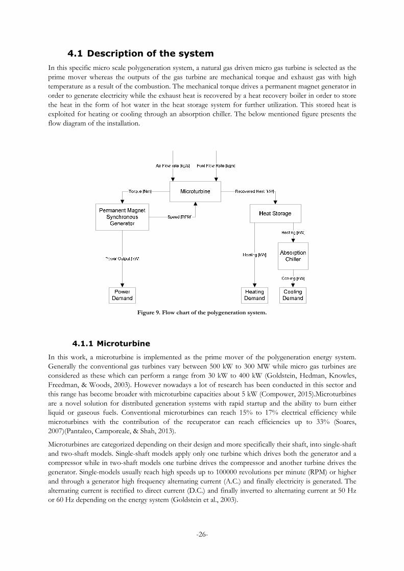
In this specific micro scale polygeneration system, a natural gas driven micro gas turbine is selected as the
prime mover whereas the outputs of the gas turbine are mechanical torque and exhaust gas with high
temperature as a result of the combustion. The mechanical torque drives a permanent magnet generator in
order to generate electricity while the exhaust heat is recovered by a heat recovery boiler in order to store
the heat in the form of hot water in the heat storage system for further utilization. This stored heat is
exploited for heating or cooling through an absorption chiller. The below mentioned figure presents the
flow diagram of the installation.
Figure 9. Flow chart of the polygeneration system.
4.1.1 Microturbine
In this work, a microturbine is implemented as the prime mover of the polygeneration energy system.
Generally the conventional gas turbines vary between 500 kW to 300 MW while micro gas turbines are
considered as these which can perform a range from 30 kW to 400 kW (Goldstein, Hedman, Knowles,
Freedman, & Woods, 2003). However nowadays a lot of research has been conducted in this sector and
this range has become broader with microturbine capacities about 5 kW (Compower, 2015).Microturbines
are a novel solution for distributed generation systems with rapid startup and the ability to burn either
liquid or gaseous fuels. Conventional microturbines can reach 15% to 17% electrical efficiency while
microturbines with the contribution of the recuperator can reach efficiencies up to 33% (Soares,
2007)(Pantaleo, Camporeale, & Shah, 2013).
Microturbines are categorized depending on their design and more specifically their shaft, into single-shaft
and two-shaft models. Single-shaft models apply only one turbine which drives both the generator and a
compressor while in two-shaft models one turbine drives the compressor and another turbine drives the
generator. Single-models usually reach high speeds up to 100000 revolutions per minute (RPM) or higher
and through a generator high frequency alternating current (A.C.) and finally electricity is generated. The
alternating current is rectified to direct current (D.C.) and finally inverted to alternating current at 50 Hz
or 60 Hz depending on the energy system (Goldstein et al., 2003).
-27-
As far as the microturbines are concerned regarding their advantages, the exhaust flue gas temperature
varies between 200 Cand350 C, which are considered as an ideal temperature range for heat supply to
residential buildings or industrial purposes. Furthermore microturbines perform fuel flexibility, consuming
either liquid or gas fuels while the low gas temperatures to the turbine inlet reduce the emissions to the
environment. Moreover microturbines are ideal for part load operation while an additional advantage is
their modularity as they can operate in parallel mode in order to supply peak loads, providing reliability to
the grid (Soares, 2007).
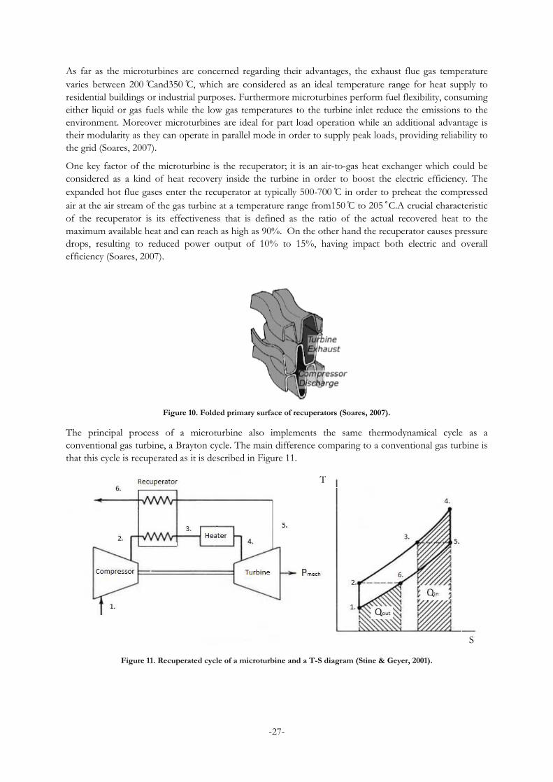
One key factor of the microturbine is the recuperator; it is an air-to-gas heat exchanger which could be
considered as a kind of heat recovery inside the turbine in order to boost the electric efficiency. The
expanded hot flue gases enter the recuperator at typically 500-700 C in order to preheat the compressed
air at the air stream of the gas turbine at a temperature range from150 C to 205 C.A crucial characteristic
of the recuperator is its effectiveness that is defined as the ratio of the actual recovered heat to the
maximum available heat and can reach as high as 90%. On the other hand the recuperator causes pressure
drops, resulting to reduced power output of 10% to 15%, having impact both electric and overall
efficiency (Soares, 2007).
Figure 10. Folded primary surface of recuperators (Soares, 2007).
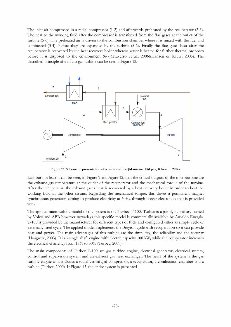
The principal process of a microturbine also implements the same thermodynamical cycle as a
conventional gas turbine, a Brayton cycle. The main difference comparing to a conventional gas turbine is
that this cycle is recuperated as it is described in Figure 11.
Figure 11. Recuperated cycle of a microturbine and a T-S diagram (Stine & Geyer, 2001).
T
S
-28-
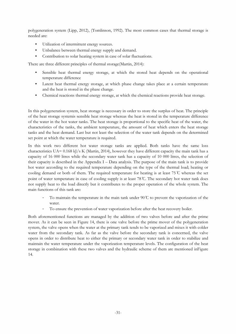
The inlet air compressed in a radial compressor (1-2) and afterwards preheated by the recuperator (2-3).
The heat to the working fluid after the compressor is transferred from the flue gases at the outlet of the
turbine (5-6). The preheated air is driven to the combustion chamber where it is mixed with the fuel and
combusted (3-4), before they are expanded by the turbine (5-6). Finally the flue gases heat after the
recuperator is recovered by the heat recovery boiler whereas water is heated for further thermal proposes
before it is disposed to the environment (6-7)(Traverso et al., 2006)(Hansen & Kautz, 2005). The
described principle of a micro gas turbine can be seen inFigure 12.
Figure 12. Schematic presentation of a microturbine (Mansouri, Nikpey, &Assadi, 2014).
Last but not least it can be seen, in Figure 9 andFigure 12, that the critical outputs of the microturbine are
the exhaust gas temperature at the outlet of the recuperator and the mechanical torque of the turbine.
After the recuperator, the exhaust gases heat is recovered by a heat recovery boiler in order to heat the
working fluid in the other stream. Regarding the mechanical torque, this drives a permanent magnet
synchronous generator, aiming to produce electricity at 50Hz through power electronics that is provided
with.
The applied microturbine model of the system is the Turbec T-100. Turbec is a jointly subsidiary owned
by Volvo and ABB however nowadays this specific model is commercially available by Ansaldo Energia.
T-100 is provided by the manufacturer for different types of fuels and configured either as simple cycle or
externally fired cycle. The applied model implements the Brayton cycle with recuperation so it can provide
heat and power. The main advantages of this turbine are the simplicity, the reliability and the security
(Haugwitz, 2003). It is a single shaft engine with electric capacity 100 kWe while the recuperator increases
the electrical efficiency from 17% to 30% (Turbec, 2009).
The main components of Turbec T-100 are gas turbine engine, electrical generator, electrical system,
control and supervision system and an exhaust gas heat exchanger. The heart of the system is the gas
turbine engine as it includes a radial centrifugal compressor, a recuperator, a combustion chamber and a
turbine (Turbec, 2009). InFigure 13, the entire system is presented.

-29-
Figure 13. Main components for Turbec T-100 PH (Turbec, 2009).
The given data in the manufacturer’s brochure are based on the ISO standard conditions (T= 15 C, P=0
Pa, RH=60%) and corresponds to the rated operational conditions as it is described in (Turbec, 2009).
The air enters the compressor and compressed with ratio 4.5 and isentropic efficiency 76.8% while the
compressor, the turbine and the generator are connected on the same shaft. The temperature of the
compressed air at the outlet of the compressor reaches 215 C and after the recuperator the temperature of
the working fluid rises to 600 C. The pressure losses in the recuperator for both gas and air streams are
about 2% whereas its effectiveness is as high as 90%.The preheated air is burnt in the combustion
chamber of 99.8% efficiency with the required fuel and the occurred flue gases from the combustion
reach 950 C at the inlet of the turbine. The gases are expanded in the turbine with a ratio of 4.5 and there
is a temperature decrease of about 300 C (Turbec, 2009)(Pantaleo et al., 2013).
The exhaust heat is recovered in order to preheat the working fluid at the compressor outlet and the
working fluid at the gas stream exits the recuperator with a temperature of 270 C. Afterwards one more
heat recovery takes place and the heat is recovered by a counter gas to fluid heat exchanger, decreasing the
temperature of the gases to 70 C. In the fluid stream of the heat exchanger water comes into with flow
rate equal to 2 l/s and the water temperature rises from 50 to 70 C, producing 165 kWth. The thermal
power input to the combustion chamber is about 333 kW and the fuel is natural gas with flow rate 0.0071
kg/s while the gases exit the heat exchanger with flow rate equal to 0.80 kg/s. As far as the other output is
concerned regarding the shaft power from the turbine, it is about 114 kW considering the mechanical
efficiency which is estimated about 98% (Turbec, 2009)(Pantaleo et al., 2013).
Table 1. Performance characteristics of Turbec T-100 (Turbec, 2009).
Performance Characteristics of Turbec T-100
Electical Output 100 (±3) kW
Electrical Efficiency 30% (±1) kW
Thermal Ouput (Hot water) 165 kW
Fuel Consumption (NG) 333 kW
Turbine Inlet Temperature 950 C
Turbine Outlet Temperature 650 C
Exhaust Gas Mass Flow ~ 0.8 kg/s
Pressure Ratio 4.5 -
Shaft Speed 70000 RPM
PMSG 2 poles
The mechanical torque of the turbine drives a high speed 2-pole permanent magnet synchronous
generator with efficiency 90% and produces high frequency AC power which is rectified and converted to

-30-
50 Hz AC power. Furthermore the power factor varies from 0.8 leading to 0.8 lagging and the rated
current is 173 A (Pantaleo et al., 2013)(Turbec, 2009).
In the following two subsections the heat exchanger and the permanent magnet synchronous generator
are discussed.
4.1.1.1 Heat exchanger
A heat exchanger is a device which absorbs and transfers heat, this process can take place between two or
more fluids which are in contact and their temperatures are different. In some heat exchangers the fluids
can be in direct contact while in other the heat exchange is done by conduction since there is a surface
which separates the fluids and they are not mixed, these devices are called recuparators. In another type of
heat exchangers the heat transfer is not continuous and they are called regenerators. Heat exchangers
categorization varies depending different characteristics and technical specifications. (Shah & Sekulic,
2006).Shell–and-tube exchangers are widely used in a variety of applications and it is key component of
this system as it increases the thermal efficiency of the plant through a heat recovery (Kozman, Kaur, &
Lee, 2009).
In this specific process a gas to water counter flow heat exchanger operates as a heat recovery boiler so it
is implemented in order to recover the heat from the exhaust gases at the outlet of the recuperator
(Turbec, 2009). The absorbed heat from the flue gases is transferred to the water which enters the fluid
side of the heat exchanger, aiming to be utilized for further heating and cooling purposes.
4.1.1.2 Generator
Microturbines result to high speeds as it is mentioned above and they usually employ one common shaft
or two shafts driving a gearbox to drive a generator. It is common these generators to be permanent
magnet synchronous generators (PMSG)(Goldstein et al., 2003).
Synchronous generators are synchronous machines which can convert the mechanical energy to
alternative electric energy. First of all a synchronous generator in order to operate, a D.C. current supply is
necessary to be induced to the rotor of the machine. This current creates a magnetic field inside the
machine while the same time the rotor is driven by an external source of mechanical power. This results to
the rotation of the magnetic field, generating a 3-phase voltage at the stator’s winding which is also the
output of the machine. Synchronous generators are an attractive and ideal solution for distributed
generation and for this reason most of the generation is comprised by synchronous generators. The
capability of reactive power generation and the high efficiency are two key factors which make them
economically preferable. Synchronous generators are categorized depending on their structure, there are
two types of generators; the wound field and permanent magnet (Elkington, 2014)(Chapman, 2005).
In this research work, a permanent magnet synchronous generator is implemented in order to produce
electricity as they are considered as suitable for distributed generation systems driven by microturbines.
The external source of mechanical power, in this case, is the mechanical torque from the gas turbine
which drives the rotor of the machine. These machines can perform high reliability and high efficiency.
Furthermore the brushless construction of a permanent magnet synchronous generator in combination
with their light weight and their small size make it a beneficial choice for a polygeneration system (Chan,
Kong, Lai, & Sciences, 2014).
4.1.2 Heat Storage
Thermal energy storage is necessary in order to decrease the wasted heat to the environment. The thermal
storage is usually short-term however it is capable to increase the thermal and overall efficiency of a
-31-
polygeneration system (Lipp, 2012), (Tomlinson, 1992). The most common cases that thermal storage is
needed are:
• Utilization of intermittent energy sources.
• Unbalance between thermal energy supply and demand.
• Contribution to solar heating system in case of solar fluctuations.
There are three different principles of thermal storage(Martin, 2014):
• Sensible heat thermal energy storage, at which the stored heat depends on the operational
temperature difference
• Latent heat thermal energy storage, at which phase change takes place at a certain temperature
and the heat is stored in the phase change.
• Chemical reactions thermal energy storage, at which the chemical reactions provide heat storage.
In this polygeneration system, heat storage is necessary in order to store the surplus of heat. The principle
of the heat storage systemis sensible heat storage whereas the heat is stored in the temperature difference
of the water in the hot water tanks. The heat storage is proportional to the specific heat of the water, the
characteristics of the tanks, the ambient temperature, the amount of heat which enters the heat storage
tanks and the heat demand. Last but not least the selection of the water tank depends on the determined
set point at which the water temperature is required.
In this work two different hot water storage tanks are applied. Both tanks have the same loss
characteristics UA= 0.168 kJ/s K (Martin, 2014), however they have different capacity the main tank has a
capacity of 16 000 litres while the secondary water tank has a capacity of 10 000 litres, the selection of
their capacity is described in the Appendix I – Data analysis. The purpose of the main tank is to provide
hot water according to the required temperature depending on the type of the thermal load; heating or
cooling demand or both of them. The required temperature for heating is at least 75 C whereas the set
point of water temperature in case of cooling supply is at least 78 C. The secondary hot water tank does
not supply heat to the load directly but it contributes to the proper operation of the whole system. The
main functions of this tank are:
- To maintain the temperature in the main tank under 90 C to prevent the vaporization of the
water.
- To ensure the prevention of water vaporization before after the heat recovery boiler.
Both aforementioned functions are managed by the addition of two valves before and after the prime
mover. As it can be seen in Figure 14, there is one valve before the prime mover of the polygeneration
system, the valve opens when the water at the primary tank tends to be vaporized and mixes it with colder
water from the secondary tank. As far as the valve before the secondary tank is concerned, the valve
opens in order to distribute heat to either the primary or secondary water tank in order to stabilize and
maintain the water temperature under the vaporization temperature levels. The configuration of the heat
storage in combination with these two valves and the hydraulic scheme of them are mentioned inFigure
14.
-32-
Figure 14. Hydraulic scheme of thermal storage.
4.1.3 Absorption chiller
Cooling systems implement the common refrigeration cycle which consists of compression, condensation,
expansion and evaporation. The mechanical compression is an efficient method, however the required
axial power input demands high quality and high cost (McQuiston & Parker, 1999). In common cooling
systems the compression requires electricity while absorption chillers require thermal energy.
Absorption chillers are a thermally efficient solution as the exhaust heat of systems like microturbines is
recovered, decreasing the wasted heat. Generally the benefits of such cooling systems are several and
comparing to the complexity of HVAC regarding its design and operation, absorption chillers could
perform high flexibility. Furthermore absorption chillers contribute to the prevention of peak electric
demand charges as well as the utilization of waste heat of a polygeneration system, for instance, can boost
the cost-effectiveness and the overall efficiency of the system(Southern California Gas Company New
Buildings Institute, 1998).
Absorption chillers are categorized into direct-fired and indirect-fired, depending on the heat source
supply and single, double or triple effect depending on the structure and the configuration of the
absorption chiller. In the direct-fired units, the heat source occurs from the combustion of gas or other
fuels inside the unit while indirect-fired while the heat source to the system is transferred from an external
source such as a boiler or recovered heat from a heat exchanger (Southern California Gas Company New
Buildings Institute, 1998).
Regarding the classification which distinguish the absorption chillers in single, double and triple effect, is
defined as following:
• Single effect, is the cycle at which the working fluid goes through the main components of a
common refrigeration machine as it can be seen in the below mentioned figure. The process
includes a generator, a condenser, an evaporator and an absorber. A single effect absorption
chiller performs low efficiency however its cost competitiveness is the main advantage of it. This
type of chillers can reach COP with a range from 0.6 to 0.8 while the working fluid entering the
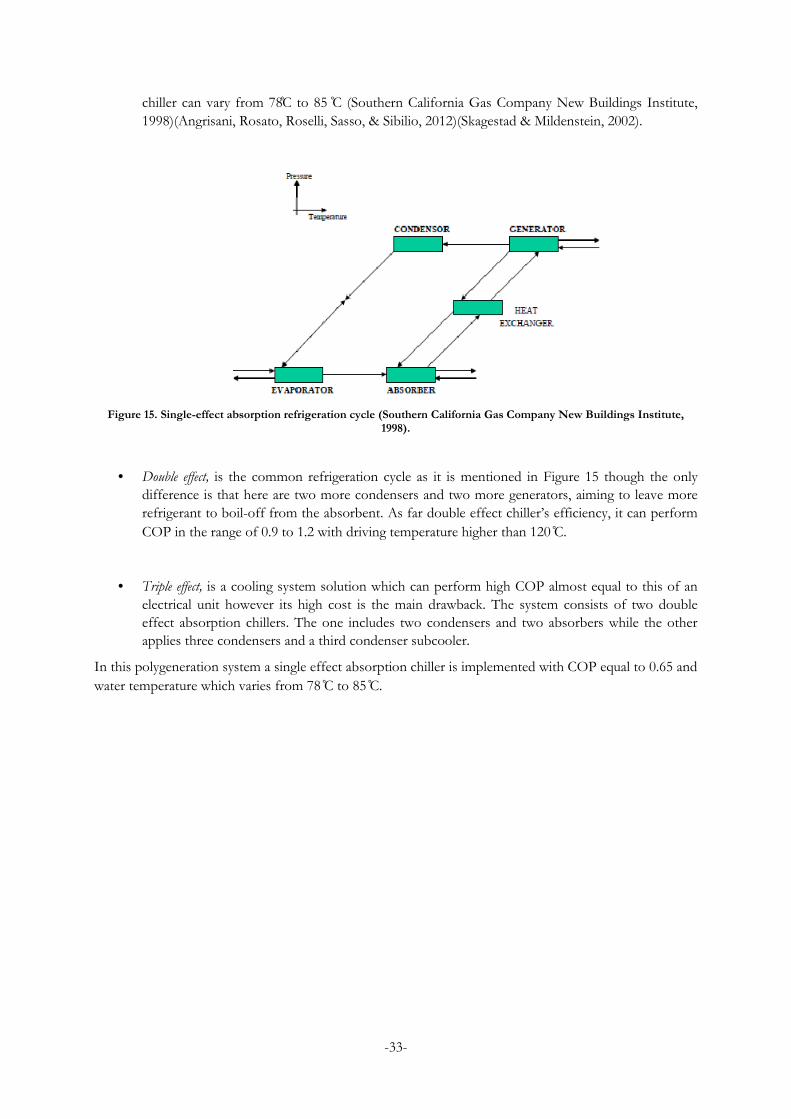
-33-
chiller can vary from 78C to 85 C (Southern California Gas Company New Buildings Institute,
1998)(Angrisani, Rosato, Roselli, Sasso, & Sibilio, 2012)(Skagestad & Mildenstein, 2002).
Figure 15. Single-effect absorption refrigeration cycle (Southern California Gas Company New Buildings Institute, 1998).
• Double effect, is the common refrigeration cycle as it is mentioned in Figure 15 though the only
difference is that here are two more condensers and two more generators, aiming to leave more
refrigerant to boil-off from the absorbent. As far double effect chiller’s efficiency, it can perform
COP in the range of 0.9 to 1.2 with driving temperature higher than 120 C.
• Triple effect, is a cooling system solution which can perform high COP almost equal to this of an
electrical unit however its high cost is the main drawback. The system consists of two double
effect absorption chillers. The one includes two condensers and two absorbers while the other
applies three condensers and a third condenser subcooler.
In this polygeneration system a single effect absorption chiller is implemented with COP equal to 0.65 and
water temperature which varies from 78 C to 85 C.

-34-
5 Modeling and control of a polygeneration system
Modeling is the representation of a system expressed by mathematical equations in order to understand its
behavior during a specific period of time. This process is important as it is used for better understanding
and analysis of the system, aiming to optimize it in the future. The analysis of the system could be referred
to interactions between the components of the system and provide information about economical and
technical issues. Some advantages are the analysis of proposed changes, identification of problems and
constraints and better investigation of the system (Single Electricity Market Operator, 2015). Last but not
least one crucial aspect of energy system modeling is the control. The control is regarded as a key factor
providing the secure operation of the system in order to ensure high reliability and high efficiency.
In this specific work, as it is explained in Chapter 2, the first step before the energy systems modeling is
the data analysis. For this reason the data extraction is discussed in this section and more specifically the
data regarding the microturbine which is considered as the ´heart´ of the system. Turbec T-100 is the only
prime mover in this polygeneration system, accordingly this chapter includes all those executed steps in
order to extract the key parameters of Turbec T-100, including the thermodynamic equations. Moreover
all the model blocks are mentioned and a discussion is made regarding the critical parameters and their set
points for each component as well as the mathematical equations which are included in the model. Finally
a test run model simulation is accomplished and the results are compared to the data of the microturbine
in order to validate the model and define the deviations from the real data.
5.1 Data analysis and mathematical equations
In this section the microturbine data is analyzed and the process for the data extraction is mentioned. This
kind of data is difficult to be found in the literature or to be provided by the manufacturer due to the
confidential data of such a system. The data is based on a previous research work (Camporeale et al.,
2014) and its simulation results as well as the Turbec T-100 brochure.
Figure 16. Gas turbine cycle (Mansouri, Nikpey, &Assadi, 2014)
In (Camporeale et al., 2014), three different scenarios are investigated, one for 100% natural gas, 50%
natural gas-50% biomass and 100% biomass, however more details are provided for the case of 100%
natural gas. Unfortunately no numerical data is given but only graphs, in the graph below the variation of
electric efficiency is presented with different electrical loads and more specifically the curve L-M-N is
chosen in order to extract data. The curve L-M-N (Lower-Medium-Nominal) represents different ranges
of the turbine speed in p.u. for different loads whereas the base value for the electric efficiency and power

-35-
are 30% and 100 kW respectively. As it has already been mentioned, the data of this work is based on the
simulation results of a previous work and this is how it could be explained that the electric efficiency is
higher than 1 in Figure 17.
Figure 17. Electrical efficiency for different electrical loads (Camporeale et al., 2014).
In Figure 17, the electrical load varies from 25 kW to 100 kW and each of them corresponds to a different
electric efficiency. For the inconvenience of the data extraction from the figures, the WebPlotDigitizer
(Rohatgi, 2015) application is applied in order to increase the precision.
Figure 18. Data extraction with WebPlotDigitizer(Rohatgi, 2015).
After taking into consideration the lower heating value (LHV) of natural gas,which is equal to 50000
kJ/kgK, and the extracted data, the fuel consumption for each load can be estimated. The fuel flow rate
can be calculated as following:
fuel f NGQ m LHV= ⋅ɺ (1.1)
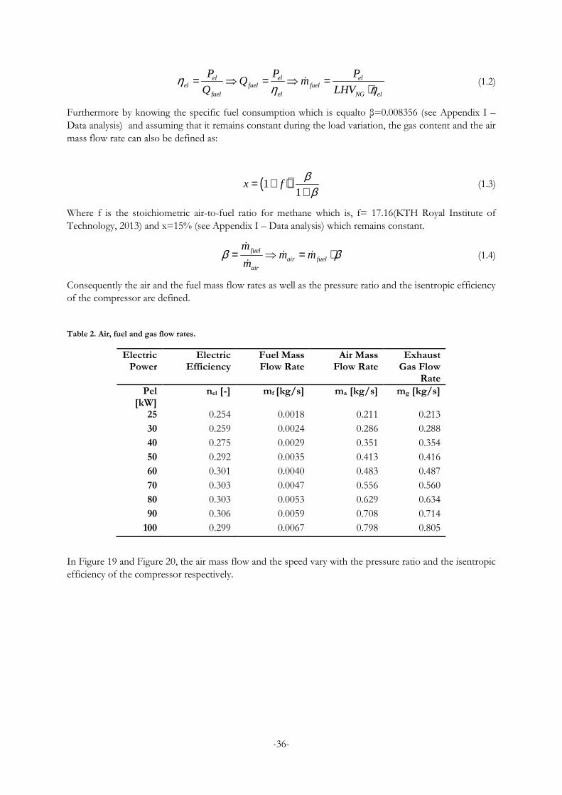
-36-
el el elel fuel fuel
fuel el NG el
P P PQ m
Q LHVη
η η= ⇒ = ⇒ =
⋅ɺ (1.2)
Furthermore by knowing the specific fuel consumption which is equalto β=0.008356 (see Appendix I –
Data analysis) and assuming that it remains constant during the load variation, the gas content and the air
mass flow rate can also be defined as:
( )11
x fβ
β= + ⋅
+ (1.3)
Where f is the stoichiometric air-to-fuel ratio for methane which is, f= 17.16(KTH Royal Institute of
Technology, 2013) and x=15% (see Appendix I – Data analysis) which remains constant.
fuel
air fuelair
mm m
mβ β= ⇒ = ⋅
ɺɺ ɺ
ɺ (1.4)
Consequently the air and the fuel mass flow rates as well as the pressure ratio and the isentropic efficiency
of the compressor are defined.
Table 2. Air, fuel and gas flow rates.
Electric Power
Electric Efficiency
Fuel Mass Flow Rate
Air Mass Flow Rate
Exhaust Gas Flow
Rate
Pel [kW]
nel [-] mf [kg/s] ma [kg/s] mg [kg/s]
25 0.254 0.0018 0.211 0.213
30 0.259 0.0024 0.286 0.288
40 0.275 0.0029 0.351 0.354
50 0.292 0.0035 0.413 0.416
60 0.301 0.0040 0.483 0.487
70 0.303 0.0047 0.556 0.560
80 0.303 0.0053 0.629 0.634
90 0.306 0.0059 0.708 0.714
100 0.299 0.0067 0.798 0.805
In Figure 19 and Figure 20, the air mass flow and the speed vary with the pressure ratio and the isentropic
efficiency of the compressor respectively.
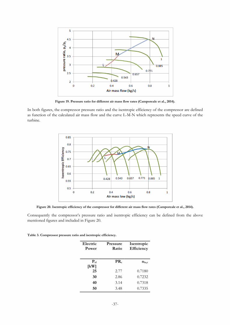
-37-
Figure 19. Pressure ratio for different air mass flow rates (Camporeale et al., 2014).
In both figures, the compressor pressure ratio and the isentropic efficiency of the compressor are defined
as function of the calculated air mass flow and the curve L-M-N which represents the speed curve of the
turbine.
Figure 20. Isentropic efficiency of the compressor for different air mass flow rates (Camporeale et al., 2014).
Consequently the compressor’s pressure ratio and isentropic efficiency can be defined from the above
mentioned figures and included in Figure 20.
Table 3. Compressor pressure ratio and isentropic efficiency.
Electric Power
Pressure Ratio
Isentropic Efficiency
Pel [kW]
PRc nis,c
25 2.77 0.7180
30 2.86 0.7232
40 3.14 0.7318
50 3.48 0.7335
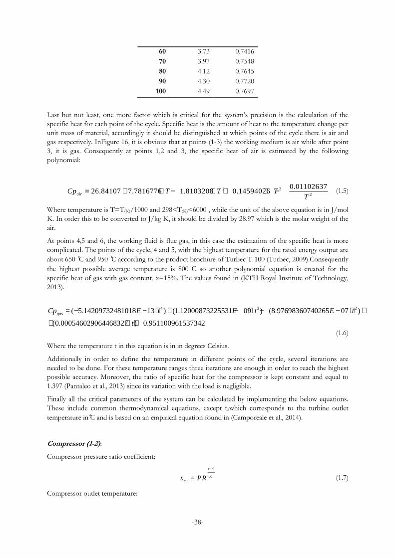
-38-
60 3.73 0.7416
70 3.97 0.7548
80 4.12 0.7645
90 4.30 0.7720
100 4.49 0.7697
Last but not least, one more factor which is critical for the system’s precision is the calculation of the
specific heat for each point of the cycle. Specific heat is the amount of heat to the temperature change per
unit mass of material, accordingly it should be distinguished at which points of the cycle there is air and
gas respectively. InFigure 16, it is obvious that at points (1-3) the working medium is air while after point
3, it is gas. Consequently at points 1,2 and 3, the specific heat of air is estimated by the following
polynomial:
2 32
0.0110263726.84107 7.7816776 1.8103208 0.14594026airCp T T T
T= + ⋅ − ⋅ + ⋅ − (1.5)
Where temperature is T=T(K)/1000 and 298<T(K)<6000 , while the unit of the above equation is in J/mol
K. In order this to be converted to J/kg K, it should be divided by 28.97 which is the molar weight of the
air.
At points 4,5 and 6, the working fluid is flue gas, in this case the estimation of the specific heat is more
complicated. The points of the cycle, 4 and 5, with the highest temperature for the rated energy output are
about 650 C and 950 C according to the product brochure of Turbec T-100 (Turbec, 2009).Consequently
the highest possible average temperature is 800 C so another polynomial equation is created for the
specific heat of gas with gas content, x=15%. The values found in (KTH Royal Institute of Technology,
2013).
4 3 2( 5.14209732481018 13 ) (1.12000873225531 09 ) (8.97698360740265 07 )
(0.000546029064468327 ) 0.951100961537342gasCp E t E t E t
t
− − ⋅ + − ⋅ −= − ⋅ +
+ ⋅ + (1.6)
Where the temperature t in this equation is in in degrees Celsius.
Additionally in order to define the temperature in different points of the cycle, several iterations are
needed to be done. For these temperature ranges three iterations are enough in order to reach the highest
possible accuracy. Moreover, the ratio of specific heat for the compressor is kept constant and equal to
1.397 (Pantaleo et al., 2013) since its variation with the load is negligible.
Finally all the critical parameters of the system can be calculated by implementing the below equations.
These include common thermodynamical equations, except t5which corresponds to the turbine outlet
temperature in C and is based on an empirical equation found in (Camporeale et al., 2014).
Compressor (1-2):
Compressor pressure ratio coefficient:
1c
ccx PR
γ
γ
−
= (1.7)
Compressor outlet temperature:
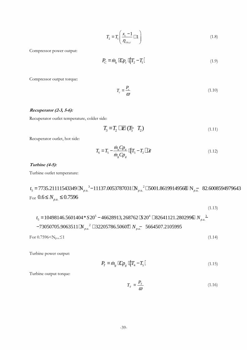
-39-
2 1
,
11c
cis c
xT T
η −= +
(1.8)
Compressor power output:
( )2 1C a cP m Cp T T= ⋅ ⋅ −ɺ (1.9)
Compressor output torque:
cc
PT
ω= (1.10)
Recuperator (2-3, 5-6):
Recuperator outlet temperature, colder side:
3 2 5 2( )T T T Tε= + ⋅ − (1.11)
Recuperator outlet, hot side:
( )6 5 5 2a a
g g
m CpT T T T
m Cpε= − ⋅ − ⋅
ɺ
ɺ (1.12)
Turbine (4-5):
Turbine outlet temperature:
3 2
5 .u. .u. .u.7735.21111543349 N 11137.0053787031 N 5001.86199149568 N 82.6008594979643p p pt = ⋅ − ⋅ + ⋅ −
For . .0.6 0.7596p uN≤ ≤
(1.13)
5 4 35 . .
2. . . .
10498146.5601404* 20 46628913,268762 20 82641121.2802996
73050705.9063511 32205786.50607 5664507.2105995
p u
p u p u
t S S N
N N
= − ⋅ + ⋅ −
− ⋅ + ⋅ −
For 0.7596<Np.u.≤1 (1.14)
Turbine power output:
( )4 5T g gP m Cp T T= ⋅ ⋅ −ɺ (1.15)
Turbine output torque:
TT
PT
ω= (1.16)

-40-
Combustion (3-4):
Energy balance is necessary at the combustion chamber in order to define the fuel mass flow rate:
4 3f comb
g g
m LHVT T
m Cp
η⋅ ⋅= +
⋅ɺ
ɺ (1.17)
Mechanical and Electrical Power:
GT T m CP P Pη= ⋅ − (1.18)
el GT genP P η= ⋅ (1.19)
Shaft Dynamics:
T C GEN mP P P T ω− − = ⋅ (1.20)
5.2 System modeling
One of the most important steps in this work was the collection and the analysis of the data. The purpose
of this process is to create a model based on a real-life system which is one of the main goals of this work.
The only necessary data in order to model this system is the gas turbine data and afterwards a validation
should ensure that the gas turbine model works properly. Regarding the other parts of the model, these
are based on common thermodynamic equations which have already been used in previous works. The
validation of a microturbine is a significant process since it was impossible to have access to a real
microturbine and due to the complexity of such a system.
As it has already been presented, modeling is the representation of a system expressed by mathematical
equations in order to understand its behavior with the time change (Single Electricity Market Operator,
2015).Accordingly the same mathematical equations are applied as these which are applied in the Data
analysis and mathematical equation section. This modeling process is mainly focused on the gas turbine
model so the model is totally based on thermodynamical equations while the system control is based on
previous research works.
The full modeling work is accomplished in Matlab/Simulink in order to develop a dynamic model.
Modeling in Simulink enhances the complexity of the model process however one important benefit is
that in Simulink a variety of systems can be modeled so it is the ideal modeling environment to integrate
models to each other. Additionally physical systems can be by mathematical models and complex
calculations can be executed quickly, being an ideal solution for dynamic models. Last but not least the
observer can have a better visualization of the entire system and block representation can show the input
and the outputs of the system (University of Michigan, 2015).
As it is described in Description of the system section, the investigated polygeneration system consists of
a microturbine, a permanent magnet synchronous generator, a heat storage system and an absorption
chiller. In this subsection the entire model is presented, the inputs and the outputs well as the key
parameters of each component are mentioned.

-41-
5.2.1 Microturbine model
Nowadays most of the gas turbine models mentioned in the literature are based on the Rowen’s model
(Rowen, 1983), whereas the main outputs are the mechanical torque and the exhaust gas temperature
while the inputs are the ambient temperature and the speed of the generator. In this work simple
thermodynamical equations are used in order to model the microturbine of the system while the same
methodology as the Rowen’s model is applied regarding the control. At this point it should be pointed
that the Rowen’s model is based on a heavy duty gas turbine which applies a simple Brayton cycle while
the gas turbine of the investigated system applies a recuperated Brayton cycle of a microturbine. Therefore
in this work the control has been modified properly by taking into consideration the work of (Guda, 2005)
whereas the Rowen’s model is applied for a microturbine.
The model consists of five parts; the thermodynamic part, the controllers; temperature and speed control,
the fuel system and the shaft dynamics. The inputs of the system are the ambient temperature and the
permanent magnet synchronous generator speed which varies depending on the electric load. The outputs
of this block are the mechanical torque, the exhaust gas temperature and the exhaust gases. The need of
control is very important as the detection of mismatches in heat flow and power, increasing the reliability
and the efficiency of the system (Murty, 2014). The speed controller controls the speed of the generator
and depending on it, the supplied fuel from the fuel system to the combustion chamber is adjusted. On
the other hand the temperature controller measures the turbine outlet temperature and compares it with a
set point value in order to define if the exhaust temperature should be reduced. In case that the exhaust
temperature exceeds the rated exhaust temperature, this is reduced by decreasing drastically the fuel flow
to the combustion chamber. Consequently the temperature control ensures the safe operation of the gas
turbine and the speed control guarantees the efficient operation and the non-interrupted supply of energy
to the load. For better understanding, a schematic Simulink block diagram has been presented in Figure
21and each block of them is analytically explained in the following sections.
Figure 21. Microturbine block diagram.
5.2.1.1 Thermodynamic part
The thermodynamic part consists of the compressor, the recuperator, the combustor and the turbine
block. This part includes thermodynamic equations, as found in (Bank Tavakoli, Vahidi, & Gawlik, 2009),
and the main inputs to this part are the ambient temperature, the speed to the compressor as well as the
fuel flow rate from the fuel system to the combustion chamber. The whole process starts with the fuel
flow rate in the combustion chamber where the air mass flow is also determined by the specific fuel
consumption which has been calculated from the data. The air mass flow and the ambient temperature
signals are sent to the compressor where both isentropic efficiency and pressure ratio are estimated,
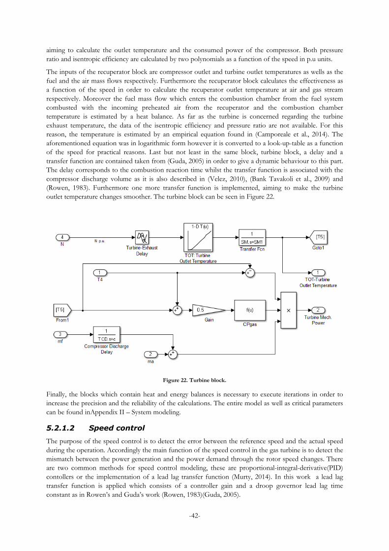
-42-
aiming to calculate the outlet temperature and the consumed power of the compressor. Both pressure
ratio and isentropic efficiency are calculated by two polynomials as a function of the speed in p.u units.
The inputs of the recuperator block are compressor outlet and turbine outlet temperatures as wells as the
fuel and the air mass flows respectively. Furthermore the recuperator block calculates the effectiveness as
a function of the speed in order to calculate the recuperator outlet temperature at air and gas stream
respectively. Moreover the fuel mass flow which enters the combustion chamber from the fuel system
combusted with the incoming preheated air from the recuperator and the combustion chamber
temperature is estimated by a heat balance. As far as the turbine is concerned regarding the turbine
exhaust temperature, the data of the isentropic efficiency and pressure ratio are not available. For this
reason, the temperature is estimated by an empirical equation found in (Camporeale et al., 2014). The
aforementioned equation was in logarithmic form however it is converted to a look-up-table as a function
of the speed for practical reasons. Last but not least in the same block, turbine block, a delay and a
transfer function are contained taken from (Guda, 2005) in order to give a dynamic behaviour to this part.
The delay corresponds to the combustion reaction time whilst the transfer function is associated with the
compressor discharge volume as it is also described in (Velez, 2010), (Bank Tavakoli et al., 2009) and
(Rowen, 1983). Furthermore one more transfer function is implemented, aiming to make the turbine
outlet temperature changes smoother. The turbine block can be seen in Figure 22.
Figure 22. Turbine block.
Finally, the blocks which contain heat and energy balances is necessary to execute iterations in order to
increase the precision and the reliability of the calculations. The entire model as well as critical parameters
can be found inAppendix II – System modeling.
5.2.1.2 Speed control
The purpose of the speed control is to detect the error between the reference speed and the actual speed
during the operation. Accordingly the main function of the speed control in the gas turbine is to detect the
mismatch between the power generation and the power demand through the rotor speed changes. There
are two common methods for speed control modeling, these are proportional-integral-derivative(PID)
contollers or the implementation of a lead lag transfer function (Murty, 2014). In this work a lead lag
transfer function is applied which consists of a controller gain and a droop governor lead lag time
constant as in Rowen’s and Guda’s work (Rowen, 1983)(Guda, 2005).
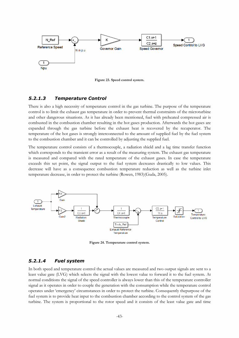
-43-
Figure 23. Speed control system.
5.2.1.3 Temperature Control
There is also a high necessity of temperature control in the gas turbine. The purpose of the temperature
control is to limit the exhaust gas temperature in order to prevent thermal constraints of the microturbine
and other dangerous situations. As it has already been mentioned, fuel with preheated compressed air is
combusted in the combustion chamber resulting in the hot gases production. Afterwards the hot gases are
expanded through the gas turbine before the exhaust heat is recovered by the recuperator. The
temperature of the hot gases is strongly interconnected to the amount of supplied fuel by the fuel system
to the combustion chamber and it can be controlled by adjusting the supplied fuel.
The temperature control consists of a thermocouple, a radiation shield and a lag time transfer function
which corresponds to the transient error as a result of the measuring system. The exhaust gas temperature
is measured and compared with the rated temperature of the exhaust gases. In case the temperature
exceeds this set point, the signal output to the fuel system decreases drastically to low values. This
decrease will have as a consequence combustion temperature reduction as well as the turbine inlet
temperature decrease, in order to protect the turbine (Rowen, 1983)(Guda, 2005).
Figure 24. Temperature control system.
5.2.1.4 Fuel system
In both speed and temperature control the actual values are measured and two output signals are sent to a
least value gate (LVG) which selects the signal with the lowest value to forward it to the fuel system. At
normal conditions the signal of the speed controller is always lower than this of the temperature controller
signal as it operates in order to couple the generation with the consumption while the temperature control
operates under ‘emergency’ circumstances in order to protect the turbine. Consequently thepurpose of the
fuel system is to provide heat input to the combustion chamber according to the control system of the gas
turbine. The system is proportional to the rotor speed and it consists of the least value gate and time

-44-
constants in series. The first time constant represents the valve positioning and the second one
corresponds to the fuel actuator (Rowen, 1983). The complete model of the fuel system can be seen in
Figure 25.
Figure 25. Fuel system control.
5.2.1.5 Shaft dynamics
In the shaft dynamics block the mechanical power of the gas turbine, the compressor and the generator
are considered as well as the mechanical efficiency of the gas turbine and the generator. The inputs are gas
turbine mechanical power and the speed of the generator while the output of the block is the mechanical
torque. The below mentioned equation has been used for the torque calculation.
T C GEN mP P P T ω− − = ⋅ (1.21)
5.2.2 Heat Recovery
Heat recovery is one of the other major components of the system. The input signal is this of the
recuperator outlet at the gas stream while one other is the water temperature coming from the heat
storage as well as gas and water mass flow rates. In the block, simple thermodynamic equations of heat
exchangers are implemented. Furthermore there are two assumptions regarding the specific heat of the gas
and the effectiveness of the heat exchanger. The effectiveness has been estimated considering the
manufacturer’s brochure (Turbec, 2009) and maintained constant at 0.9 during the load changes. Since the
specific heat is also has been calculated and kept constant at 1.0308 kJ/kgK, the range of temperature
difference during the load changes is negligible. The outputs of the block are the amount of the recovered
heat, the temperature of the water exiting the recuperator and entering the heat storage as well as the
temperature of the exhaust gases dumped to the environment. Last but not least, the gas mass flow varies
with different electrical loads while the water mass flow to the heat recovery unit is assumed to be
constant (4 l/s). The aforementioned equations are implemented in the block.
7 6 6(T T)sT T ε= − ⋅ − (1.22)
8 6 s(T T )g gs
w w
m CpT T
m Cpε
⋅= + ⋅ ⋅ −
⋅ɺ
ɺ (1.23)
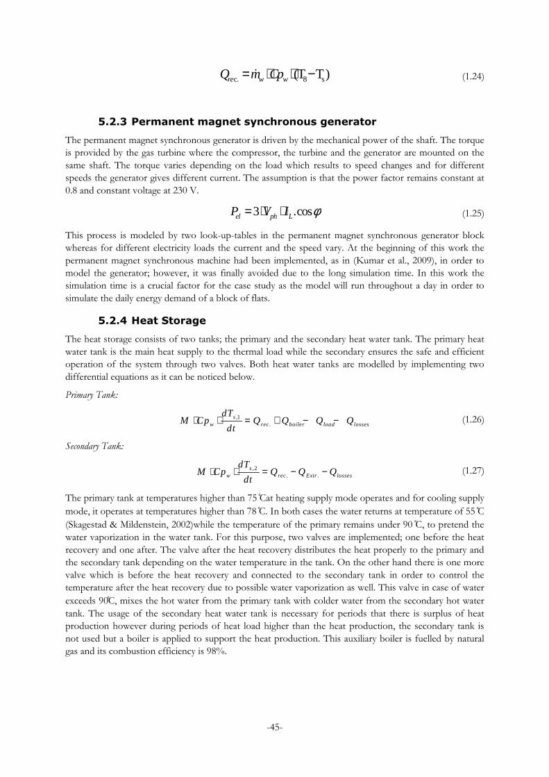
-45-
c. 8 s(T T)re w wQ m Cp= ⋅ ⋅ −ɺ (1.24)
5.2.3 Permanent magnet synchronous generator
The permanent magnet synchronous generator is driven by the mechanical power of the shaft. The torque
is provided by the gas turbine where the compressor, the turbine and the generator are mounted on the
same shaft. The torque varies depending on the load which results to speed changes and for different
speeds the generator gives different current. The assumption is that the power factor remains constant at
0.8 and constant voltage at 230 V.
3 .cosel ph LP V I φ= ⋅ ⋅ (1.25)
This process is modeled by two look-up-tables in the permanent magnet synchronous generator block
whereas for different electricity loads the current and the speed vary. At the beginning of this work the
permanent magnet synchronous machine had been implemented, as in (Kumar et al., 2009), in order to
model the generator; however, it was finally avoided due to the long simulation time. In this work the
simulation time is a crucial factor for the case study as the model will run throughout a day in order to
simulate the daily energy demand of a block of flats.
5.2.4 Heat Storage
The heat storage consists of two tanks; the primary and the secondary heat water tank. The primary heat
water tank is the main heat supply to the thermal load while the secondary ensures the safe and efficient
operation of the system through two valves. Both heat water tanks are modelled by implementing two
differential equations as it can be noticed below.
Primary Tank:
,1.
sw rec boiler load losses
dTM Cp Q Q Q Q
dt⋅ ⋅ = + − − (1.26)
Secondary Tank:
,2. .
sw rec Extr losses
dTM Cp Q Q Q
dt⋅ ⋅ = − − (1.27)
The primary tank at temperatures higher than 75 Cat heating supply mode operates and for cooling supply
mode, it operates at temperatures higher than 78 C. In both cases the water returns at temperature of 55 C
(Skagestad & Mildenstein, 2002)while the temperature of the primary remains under 90 C, to pretend the
water vaporization in the water tank. For this purpose, two valves are implemented; one before the heat
recovery and one after. The valve after the heat recovery distributes the heat properly to the primary and
the secondary tank depending on the water temperature in the tank. On the other hand there is one more
valve which is before the heat recovery and connected to the secondary tank in order to control the
temperature after the heat recovery due to possible water vaporization as well. This valve in case of water
exceeds 90C, mixes the hot water from the primary tank with colder water from the secondary hot water
tank. The usage of the secondary heat water tank is necessary for periods that there is surplus of heat
production however during periods of heat load higher than the heat production, the secondary tank is
not used but a boiler is applied to support the heat production. This auxiliary boiler is fuelled by natural
gas and its combustion efficiency is 98%.
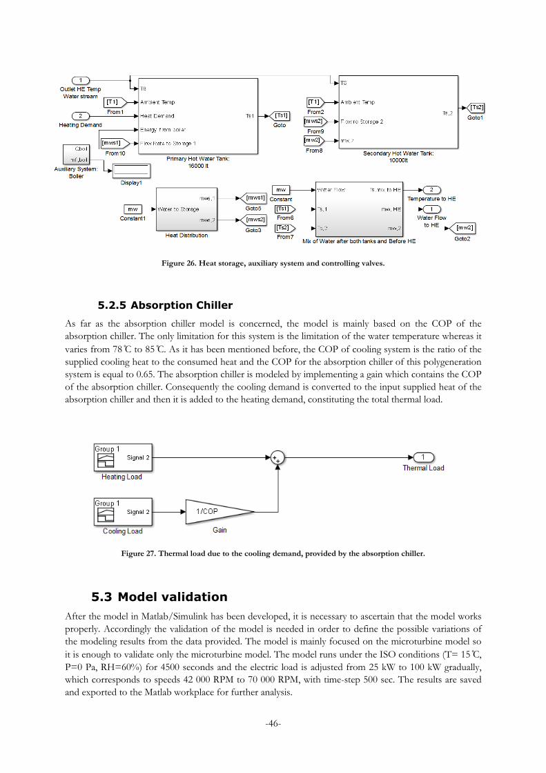
-46-
Figure 26. Heat storage, auxiliary system and controlling valves.
5.2.5 Absorption Chiller
As far as the absorption chiller model is concerned, the model is mainly based on the COP of the
absorption chiller. The only limitation for this system is the limitation of the water temperature whereas it
varies from 78 C to 85 C. As it has been mentioned before, the COP of cooling system is the ratio of the
supplied cooling heat to the consumed heat and the COP for the absorption chiller of this polygeneration
system is equal to 0.65. The absorption chiller is modeled by implementing a gain which contains the COP
of the absorption chiller. Consequently the cooling demand is converted to the input supplied heat of the
absorption chiller and then it is added to the heating demand, constituting the total thermal load.
Figure 27. Thermal load due to the cooling demand, provided by the absorption chiller.
5.3 Model validation
After the model in Matlab/Simulink has been developed, it is necessary to ascertain that the model works
properly. Accordingly the validation of the model is needed in order to define the possible variations of
the modeling results from the data provided. The model is mainly focused on the microturbine model so
it is enough to validate only the microturbine model. The model runs under the ISO conditions (T= 15 C,
P=0 Pa, RH=60%) for 4500 seconds and the electric load is adjusted from 25 kW to 100 kW gradually,
which corresponds to speeds 42 000 RPM to 70 000 RPM, with time-step 500 sec. The results are saved
and exported to the Matlab workplace for further analysis.

-47-
In this analysis the data from the literature study are compared with the modeling results and error factors
are estimated in order to define the error deviation and consider the possible error in future simulations.
Figure 28. Points specification for validation test run.
For practical reasons, each point corresponds to a certain speed as it can be seen in Figure 28. In the
following figure the electric efficiency is presented for each point, compared with the modeling results as
well as power the factors are included. The validations results, the comparison with the data and the
investigation of the error factors lead to the conclusion that the model works properly since the highest
error factor is 2.1%.
An important factor which could be investigated in order to determine the reliability of the model is the
electrical efficiency. The electrical efficiency is defined as the ratio of the produced electric power to the
input heat of the microturbine. As it can be noticed in Figure 29, the electric efficiency increases gradually
from 25% at point 2 to 30.6% at point 7. Furthermore from point 7 to point 9 the electric efficiency
decreases to 30% while at point 1 the electric efficiency reaches 28.5%. It should be emphasized that at
point 7, the highest error factor is 2.1% of the entire simulation process.
Figure 29. Modeling results of the electric efficiency compared with data and error factors.
40000
45000
50000
55000
60000
65000
70000
75000
0 1 2 3 4 5 6 7 8 9 10
Sp
eed
[R
PM
]
Points
Points Specification
0
5
10
15
20
25
30
35
0 1 2 3 4 5 6 7 8 9 10
Ele
ctri
c E
ffic
ien
cy [
%]
Points
Electric Efficiency
Data
Model
Points N
- [RPM]
1 42000
2 45990
3 47586
4 53172
5 57960
6 61950
7 63963
8 67988
9 70000
F El. Efficiency EF
- Data Modeled %
1 28.477 28.487 0.036
2 25.201 25.195 0.023 3 27.651 27.702 0.185
4 29.038 28.974 0.222
5 29.906 30.069 0.547
6 30.168 29.886 0.935
7 30.610 31.252 2.099
8 30.539 30.467 0.237
9 30.038 30.028 0.031

-48-
As it can be noticed, the point 1 seems not to be correct however this is what was simulated, by taking
into consideration the given data. One possibility could be that the model does not work properly
however if the error factor at point one is considered, it will be seen that the error between the data and
the modeling results is 0.03%. Consequently the model works properly while the main reason of this
mismatch with the other points could be due to the data since it is based on a previous research work and
its simulation results.
Finally one more observation of high significance is that the turbine reaches the highest electric efficiency
at point 7 however the error is 2.1%. On the other hand the second highest electric efficiency is equal to
30.5% and reached at point 8 whereas the error is close -0.2%. The points 7 and 8 correspond to 63 963
RPM and 67 988 RPM respectively where the power output of the machine is 80% and 90% of the rated
electric power output. Therefore the most efficient operation of this specific microturbine can be achieved
when it operates between 80% and 90% of its rated power output.

-49-
6 The case study
In the previous chapters theoretical and technical perspectives of polygeneration systems are mentioned as
well as more specifically the polygeneration system of this work and its components. Furthermore all the
critical parameters and the model of the system including the control are presented. Moreover the model
is validated and the most efficient operating points are defined. The next step of this work is the energy
monitor of a residential area, the energy supply of this area and the operational strategy of the
polygeneration system.
After taking into consideration the design of this polygeneration system, a data analysis is executed in
order to create the load curves of electricity, heating and cooling demand. The investigated system consists
of a microturbine, a heat recovery, a heat storage system and an absorption chiller. As it can be noticed
from the design of this system the first priority from the energy demand point of view is the electricity.
The supplied fuel to the system depends on the electricity demand and following the electricity demand, a
proportional amount of heat is available for recovery. Therefore the selection of the load could be
achieved by considering the electric capacity of the entire polygeneration so the electric capacity of the
microturbine. The polygeneration system and the microturbine are provided without electricity storage so
it should be ensured that the microturbine could supply electricity to the load throughout the day. The
electric capacity of the microturbine is 100kWe, accordingly the selected load should have electricity
demand up to 100 kWe. As far as the thermal demand is concerned, the produced thermal energy depends
on the electricity demand, for this reason the polygeneration system is provided with heat storage system
and an auxiliary boiler. Consequently thermal energy is stored in case the heat production is higher than
the demand or an auxiliary boiler supplies the thermal load in case that the heat demand is higher than the
produced and stored heat. Last but not least two cases should be investigated in order to show the
behavior of the system during winter (January) when heating is required and one other during the summer
(August) when there is only cooling demand.For this reason, the load is assumed that it is located in North
Italy and more specifically in the area of Milan where the climate conditions could allow this work to show
undoubtedly what happens during the two aforementioned periods of the year.
This chapter includes all the implemented steps in order to define the load demand and the load curve
creation as well as the results of two model simulations for twenty four hours during January and August
in Milan, Italy.
6.1 Electric, heating and cooling demand
In(Bianchi, Pascale, Melino, & Peretto, 2014), the curves for both electric and heating loads have been
created. Both load curves are referred to a residential building in Italy and they are normalized depending
on the rated capacity of the system. Furthermore regarding the electric demand, it varies depending the
period of the year and more specifically two different curves are given; one for the summer and one for
the winter, as it can be seen in Figure 30.
Figure 30. Normalized curve of hourly electric load in (a) winter, (b) summer.
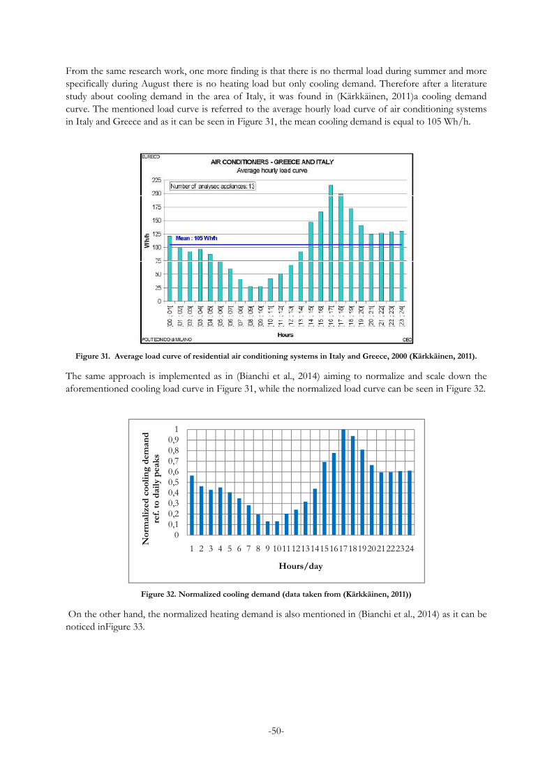
-50-
From the same research work, one more finding is that there is no thermal load during summer and more
specifically during August there is no heating load but only cooling demand. Therefore after a literature
study about cooling demand in the area of Italy, it was found in (Kärkkäinen, 2011)a cooling demand
curve. The mentioned load curve is referred to the average hourly load curve of air conditioning systems
in Italy and Greece and as it can be seen in Figure 31, the mean cooling demand is equal to 105 Wh/h.
Figure 31. Average load curve of residential air conditioning systems in Italy and Greece, 2000 (Kärkkäinen, 2011).
The same approach is implemented as in (Bianchi et al., 2014) aiming to normalize and scale down the
aforementioned cooling load curve in Figure 31, while the normalized load curve can be seen in Figure 32.
Figure 32. Normalized cooling demand (data taken from (Kärkkäinen, 2011))
On the other hand, the normalized heating demand is also mentioned in (Bianchi et al., 2014) as it can be
noticed inFigure 33.
00,10,20,30,40,50,60,70,80,9
1
1 2 3 4 5 6 7 8 9 101112131415161718192021222324
No
rmali
zed
co
oli
ng
dem
an
d
ref.
to
dail
y p
eak
s
Hours/day

-51-
Figure 33. Normalized heating demand (Bianchi et al., 2014).
The next step in order to create the demand curves is to determine the demand of this specific
polygeneration system. For this system the electric capacity of the microturbine is applied to Figure 30 and
defined that this system can provide with electricity 95 apartments with an average of 4 residents per
apartment and average annual consumption 4628kWh according to(Zimmermann et al., 2012). InFigure
34 and Figure 35, the daily electric demand in January and August can be seen.
Figure 34. Hourly electric demand per day, January.
0
0,1
0,2
0,3
0,4
0,5
0,6
0,7
0,8
0,9
1
1 2 3 4 5 6 7 8 9 10 11 12 13 14 15 16 17 18 19 20 21 22 23 24
No
rmali
zed
hea
tin
g d
eman
d
ref.
to
dail
y p
eak
s
Hours/day
0
10
20
30
40
50
60
70
80
90
100
1 2 3 4 5 6 7 8 9 101112131415161718192021222324
Ele
ctri
c d
eman
d i
n k
W
Hours/day
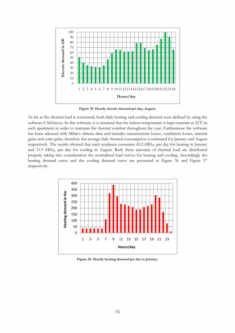
-52-
Figure 35. Hourly electric demand per day, August.
As far as the thermal load is concerned, both daily heating and cooling demand were defined by using the
software CASAnova. In this software, it is assumed that the indoor temperature is kept constant at 22 C in
each apartment in order to maintain the thermal comfort throughout the year. Furthermore the software
has been adjusted with Milan’s climate data and includes transmissions losses, ventilation losses, internal
gains and solar gains, therefore the average daily thermal consumption is estimated for January and August
respectively. The results showed that each residence consumes 43.2 kWhth per day for heating in January
and 11.9 kWhth per day for cooling in August. Both these amounts of thermal load are distributed
properly taking into consideration the normalized load curves for heating and cooling. Accordingly the
heating demand curve and the cooling demand curve are presented in Figure 36 and Figure 37
respectively.
Figure 36. Hourly heating demand per day in January.
0
10
20
30
40
50
60
70
80
90
100
1 2 3 4 5 6 7 8 9 101112131415161718192021222324
Ele
ctri
c d
eman
d i
n k
W
Hours/day
0
50
100
150
200
250
300
350
400
1 3 5 7 9 11 13 15 17 19 21 23
He
ati
ng
de
ma
nd
in
Kw
Hours/day
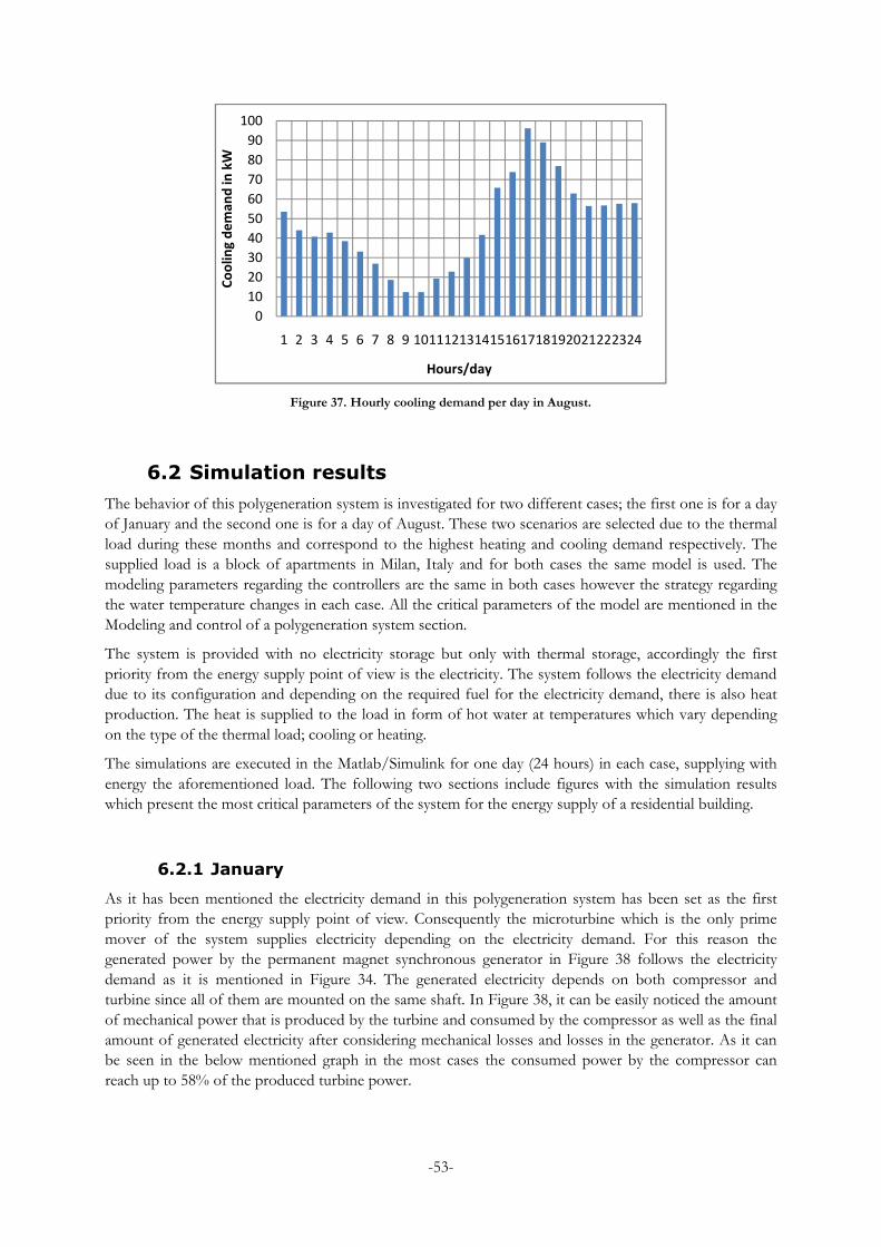
-53-
Figure 37. Hourly cooling demand per day in August.
6.2 Simulation results
The behavior of this polygeneration system is investigated for two different cases; the first one is for a day
of January and the second one is for a day of August. These two scenarios are selected due to the thermal
load during these months and correspond to the highest heating and cooling demand respectively. The
supplied load is a block of apartments in Milan, Italy and for both cases the same model is used. The
modeling parameters regarding the controllers are the same in both cases however the strategy regarding
the water temperature changes in each case. All the critical parameters of the model are mentioned in the
Modeling and control of a polygeneration system section.
The system is provided with no electricity storage but only with thermal storage, accordingly the first
priority from the energy supply point of view is the electricity. The system follows the electricity demand
due to its configuration and depending on the required fuel for the electricity demand, there is also heat
production. The heat is supplied to the load in form of hot water at temperatures which vary depending
on the type of the thermal load; cooling or heating.
The simulations are executed in the Matlab/Simulink for one day (24 hours) in each case, supplying with
energy the aforementioned load. The following two sections include figures with the simulation results
which present the most critical parameters of the system for the energy supply of a residential building.
6.2.1 January
As it has been mentioned the electricity demand in this polygeneration system has been set as the first
priority from the energy supply point of view. Consequently the microturbine which is the only prime
mover of the system supplies electricity depending on the electricity demand. For this reason the
generated power by the permanent magnet synchronous generator in Figure 38 follows the electricity
demand as it is mentioned in Figure 34. The generated electricity depends on both compressor and
turbine since all of them are mounted on the same shaft. In Figure 38, it can be easily noticed the amount
of mechanical power that is produced by the turbine and consumed by the compressor as well as the final
amount of generated electricity after considering mechanical losses and losses in the generator. As it can
be seen in the below mentioned graph in the most cases the consumed power by the compressor can
reach up to 58% of the produced turbine power.
0
10
20
30
40
50
60
70
80
90
100
1 2 3 4 5 6 7 8 9 101112131415161718192021222324
Co
oli
ng
de
ma
nd
in k
W
Hours/day
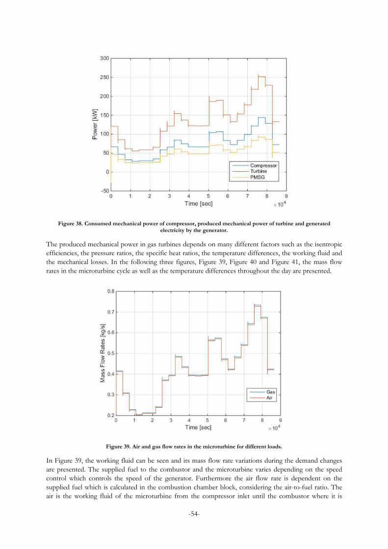
-54-
Figure 38. Consumed mechanical power of compressor, produced mechanical power of turbine and generated electricity by the generator.
The produced mechanical power in gas turbines depends on many different factors such as the isentropic
efficiencies, the pressure ratios, the specific heat ratios, the temperature differences, the working fluid and
the mechanical losses. In the following three figures, Figure 39, Figure 40 and Figure 41, the mass flow
rates in the microturbine cycle as well as the temperature differences throughout the day are presented.
Figure 39. Air and gas flow rates in the microturbine for different loads.
In Figure 39, the working fluid can be seen and its mass flow rate variations during the demand changes
are presented. The supplied fuel to the combustor and the microturbine varies depending on the speed
control which controls the speed of the generator. Furthermore the air flow rate is dependent on the
supplied fuel which is calculated in the combustion chamber block, considering the air-to-fuel ratio. The
air is the working fluid of the microturbine from the compressor inlet until the combustor where it is
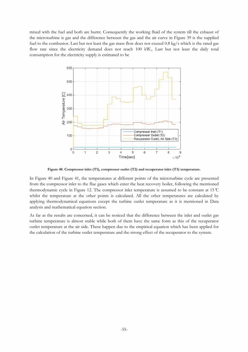
-55-
mixed with the fuel and both are burnt. Consequently the working fluid of the system till the exhaust of
the microturbine is gas and the difference between the gas and the air curve in Figure 39 is the supplied
fuel to the combustor. Last but not least the gas mass flow does not exceed 0.8 kg/s which is the rated gas
flow rate since the electricity demand does not reach 100 kWe. Last but not least the daily total
consumption for the electricity supply is estimated to be
Figure 40. Compressor inlet (T1), compressor outlet (T2) and recuperator inlet (T3) temperature.
In Figure 40 and Figure 41, the temperatures at different points of the microturbine cycle are presented
from the compressor inlet to the flue gases which enter the heat recovery boiler, following the mentioned
thermodynamic cycle in Figure 12. The compressor inlet temperature is assumed to be constant at 15 C
whilst the temperature at the other points is calculated. All the other temperatures are calculated by
applying thermodynamical equations except the turbine outlet temperature as it is mentioned in Data
analysis and mathematical equation section.
As far as the results are concerned, it can be noticed that the difference between the inlet and outlet gas
turbine temperature is almost stable while both of them have the same form as this of the recuperator
outlet temperature at the air side. These happen due to the empirical equation which has been applied for
the calculation of the turbine outlet temperature and the strong effect of the recuperator to the system.
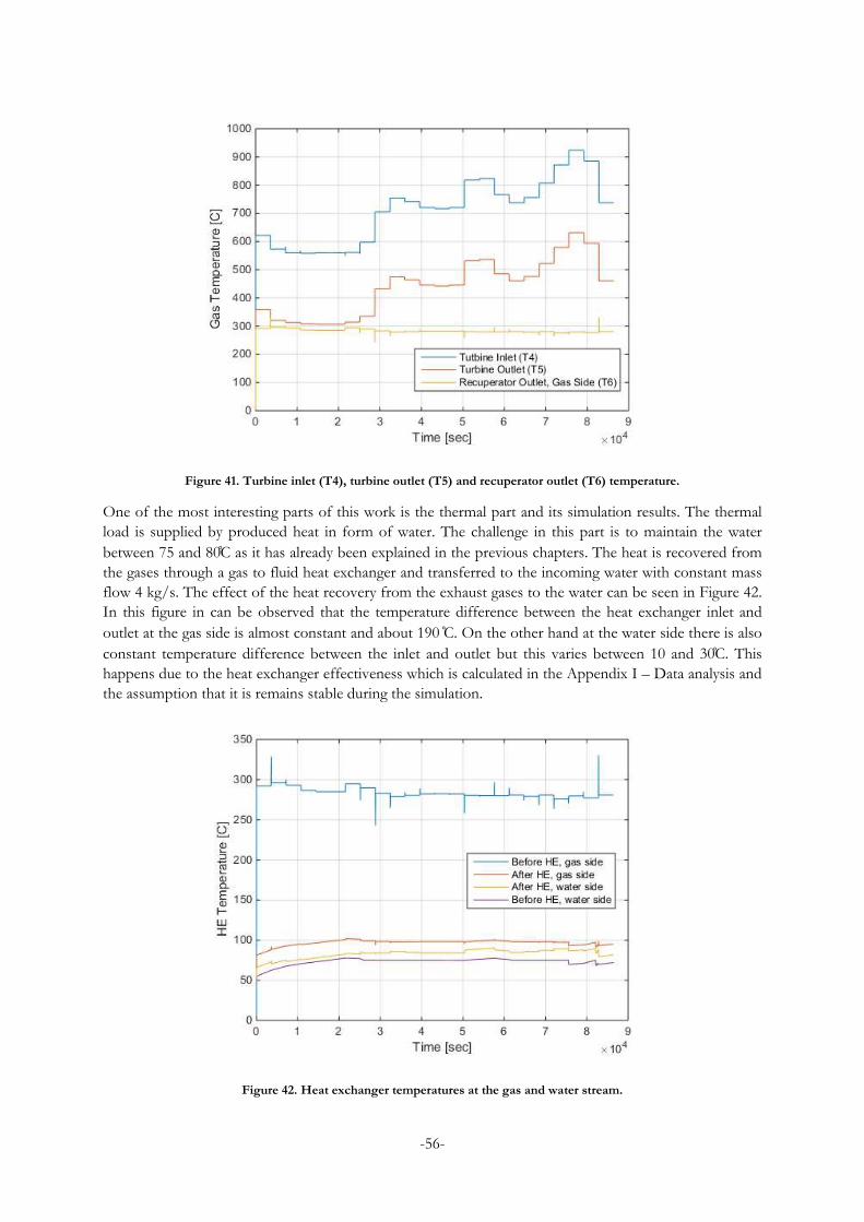
-56-
Figure 41. Turbine inlet (T4), turbine outlet (T5) and recuperator outlet (T6) temperature.
One of the most interesting parts of this work is the thermal part and its simulation results. The thermal
load is supplied by produced heat in form of water. The challenge in this part is to maintain the water
between 75 and 80C as it has already been explained in the previous chapters. The heat is recovered from
the gases through a gas to fluid heat exchanger and transferred to the incoming water with constant mass
flow 4 kg/s. The effect of the heat recovery from the exhaust gases to the water can be seen in Figure 42.
In this figure in can be observed that the temperature difference between the heat exchanger inlet and
outlet at the gas side is almost constant and about 190 C. On the other hand at the water side there is also
constant temperature difference between the inlet and outlet but this varies between 10 and 30 C. This
happens due to the heat exchanger effectiveness which is calculated in the Appendix I – Data analysis and
the assumption that it is remains stable during the simulation.
Figure 42. Heat exchanger temperatures at the gas and water stream.
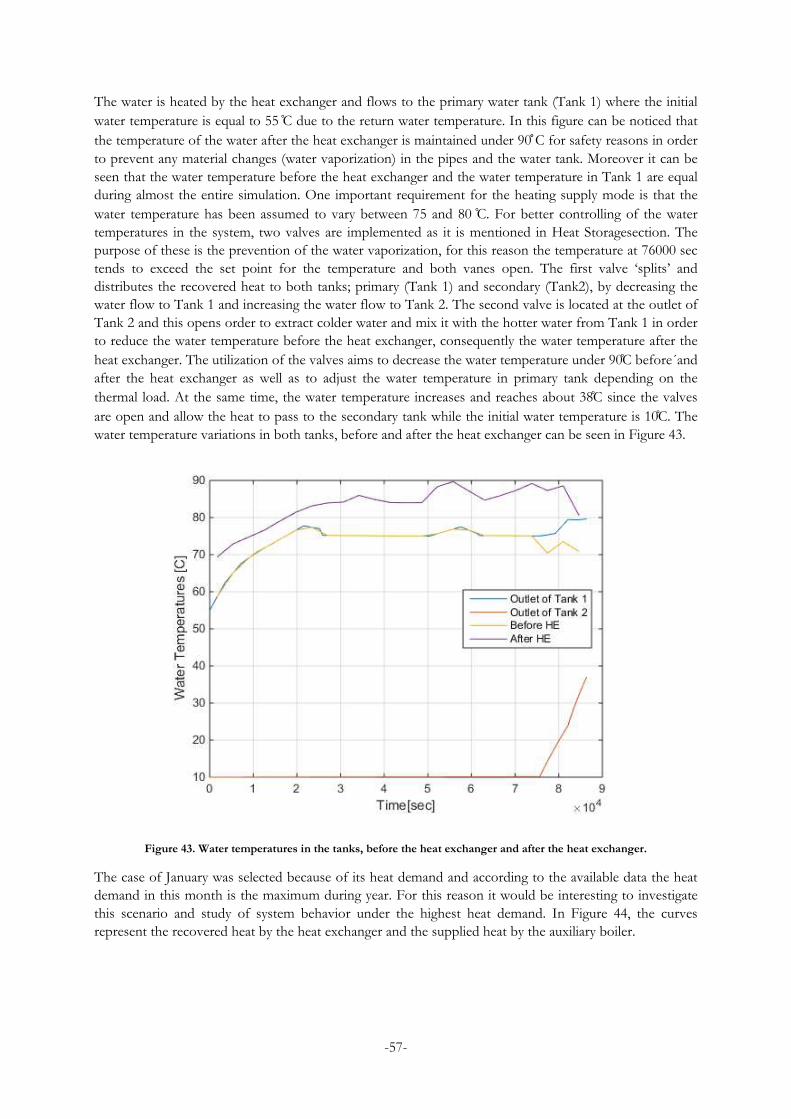
-57-
The water is heated by the heat exchanger and flows to the primary water tank (Tank 1) where the initial
water temperature is equal to 55 C due to the return water temperature. In this figure can be noticed that
the temperature of the water after the heat exchanger is maintained under 90 C for safety reasons in order
to prevent any material changes (water vaporization) in the pipes and the water tank. Moreover it can be
seen that the water temperature before the heat exchanger and the water temperature in Tank 1 are equal
during almost the entire simulation. One important requirement for the heating supply mode is that the
water temperature has been assumed to vary between 75 and 80 C. For better controlling of the water
temperatures in the system, two valves are implemented as it is mentioned in Heat Storagesection. The
purpose of these is the prevention of the water vaporization, for this reason the temperature at 76000 sec
tends to exceed the set point for the temperature and both vanes open. The first valve ‘splits’ and
distributes the recovered heat to both tanks; primary (Tank 1) and secondary (Tank2), by decreasing the
water flow to Tank 1 and increasing the water flow to Tank 2. The second valve is located at the outlet of
Tank 2 and this opens order to extract colder water and mix it with the hotter water from Tank 1 in order
to reduce the water temperature before the heat exchanger, consequently the water temperature after the
heat exchanger. The utilization of the valves aims to decrease the water temperature under 90C before´and
after the heat exchanger as well as to adjust the water temperature in primary tank depending on the
thermal load. At the same time, the water temperature increases and reaches about 38C since the valves
are open and allow the heat to pass to the secondary tank while the initial water temperature is 10C. The
water temperature variations in both tanks, before and after the heat exchanger can be seen in Figure 43.
Figure 43. Water temperatures in the tanks, before the heat exchanger and after the heat exchanger.
The case of January was selected because of its heat demand and according to the available data the heat
demand in this month is the maximum during year. For this reason it would be interesting to investigate
this scenario and study of system behavior under the highest heat demand. In Figure 44, the curves
represent the recovered heat by the heat exchanger and the supplied heat by the auxiliary boiler.

-58-
Figure 44. Recovered heat by the heat exchanger and additional supplied het by the auxiliary boiler.
From the aforementioned figure, it can be seen that almost the 24.5% percent of the heat demand is
supplied by the auxiliary boiler The daily heat demand is 4 100 kWh and it is estimated that the heat
supply from the auxiliary system will result to 4500 kg of natural gas in addition to this which is consumed
for the electricity generation. This amount of additional natural gas is equivalent to 47.4 kg/day per
household while the total fuel consumption is estimated to be 241.2 kg/day per household.
The boiler operates in order to maintain the water temperature at lowest possible water temperature which
is suitable for heating. In this case the this temperature is equal to 75 C and for this reason it can be
noticed in Figure 43 that when the auxiliary boiler operates at 26 000 sec the water temperature in Tank 1
remains stable at 75C. However when the recovered heat is more than the heat demand and the boiler
does not supply the load the water temperature varies at temperatures higher than 75 C.
6.2.2 August
Regarding the case of August, the first priority of the system from the energy supply point of view is the
electricity demand like the case of January, though the thermal load is cooling demand. Due to the
electricity demand as first priority, the microturbine follows the electric load as it can be seen in Figure 45.
Accordingly the generated electricity by the generator also corresponds to the electricity demand and it
can be noticed that the period between 76 800 and 80 000 sec, the generator reaches the rated electric
production which is 100 kWe. Regarding the compressor’s power consumption and the turbine produced
power, the same losses and efficiencies have been applied as the case of January. All these can be found in
the Appendix. As it has already been discussed in the case of January, it can also be seen in Figure 45,
where the case of August is included, that the consumed mechanical power of the compressor almost
reaches the 60% of the produced turbine power.
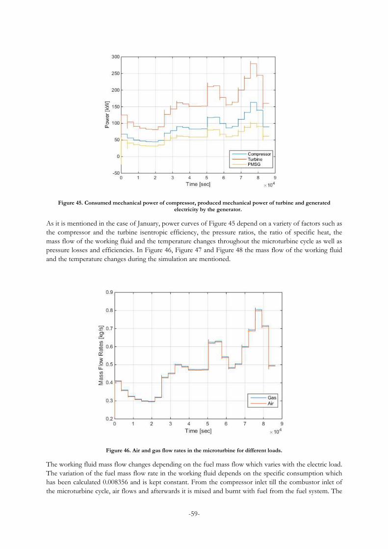
-59-
Figure 45. Consumed mechanical power of compressor, produced mechanical power of turbine and generated electricity by the generator.
As it is mentioned in the case of January, power curves of Figure 45 depend on a variety of factors such as
the compressor and the turbine isentropic efficiency, the pressure ratios, the ratio of specific heat, the
mass flow of the working fluid and the temperature changes throughout the microturbine cycle as well as
pressure losses and efficiencies. In Figure 46, Figure 47 and Figure 48 the mass flow of the working fluid
and the temperature changes during the simulation are mentioned.
Figure 46. Air and gas flow rates in the microturbine for different loads.
The working fluid mass flow changes depending on the fuel mass flow which varies with the electric load.
The variation of the fuel mass flow rate in the working fluid depends on the specific consumption which
has been calculated 0.008356 and is kept constant. From the compressor inlet till the combustor inlet of
the microturbine cycle, air flows and afterwards it is mixed and burnt with fuel from the fuel system. The
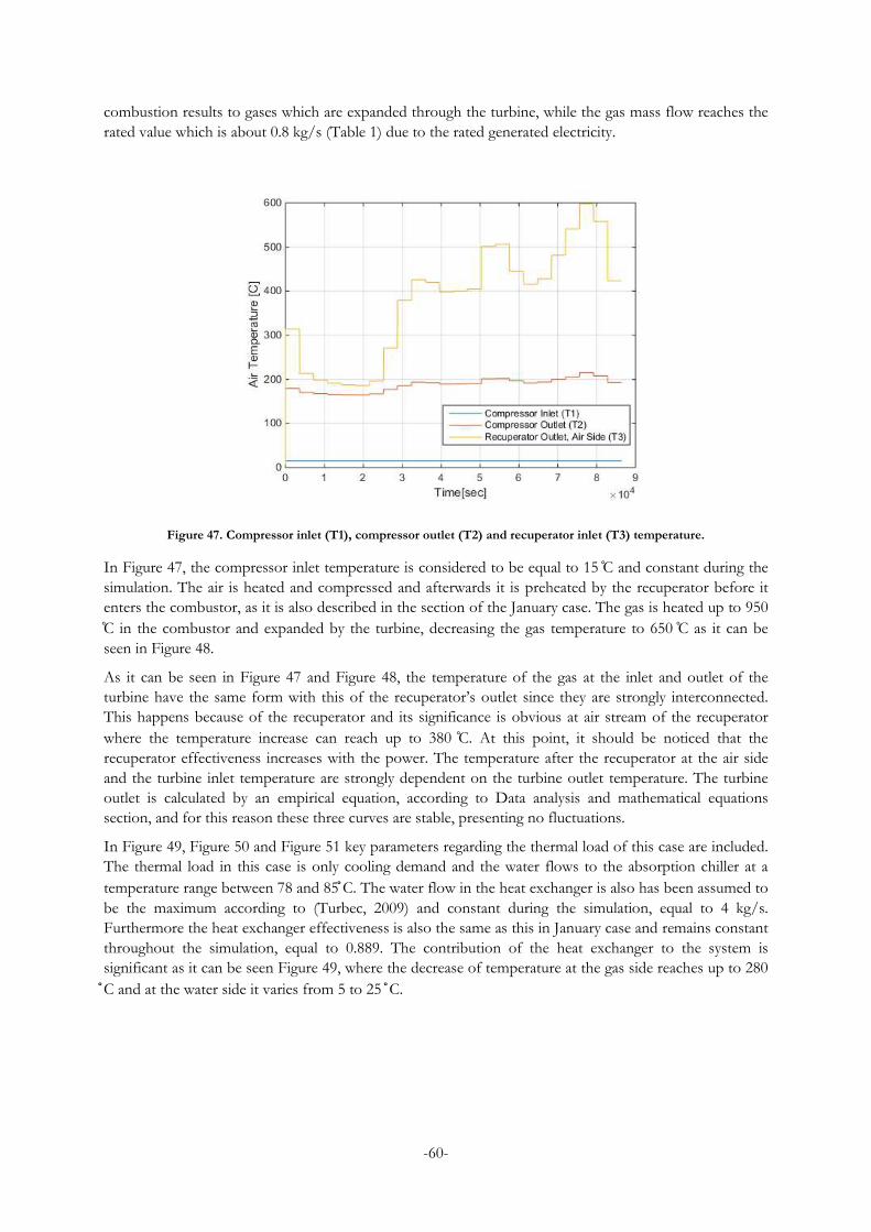
-60-
combustion results to gases which are expanded through the turbine, while the gas mass flow reaches the
rated value which is about 0.8 kg/s (Table 1) due to the rated generated electricity.
Figure 47. Compressor inlet (T1), compressor outlet (T2) and recuperator inlet (T3) temperature.
In Figure 47, the compressor inlet temperature is considered to be equal to 15 C and constant during the
simulation. The air is heated and compressed and afterwards it is preheated by the recuperator before it
enters the combustor, as it is also described in the section of the January case. The gas is heated up to 950
C in the combustor and expanded by the turbine, decreasing the gas temperature to 650 C as it can be
seen in Figure 48.
As it can be seen in Figure 47 and Figure 48, the temperature of the gas at the inlet and outlet of the
turbine have the same form with this of the recuperator’s outlet since they are strongly interconnected.
This happens because of the recuperator and its significance is obvious at air stream of the recuperator
where the temperature increase can reach up to 380 C. At this point, it should be noticed that the
recuperator effectiveness increases with the power. The temperature after the recuperator at the air side
and the turbine inlet temperature are strongly dependent on the turbine outlet temperature. The turbine
outlet is calculated by an empirical equation, according to Data analysis and mathematical equations
section, and for this reason these three curves are stable, presenting no fluctuations.
In Figure 49, Figure 50 and Figure 51 key parameters regarding the thermal load of this case are included.
The thermal load in this case is only cooling demand and the water flows to the absorption chiller at a
temperature range between 78 and 85 C. The water flow in the heat exchanger is also has been assumed to
be the maximum according to (Turbec, 2009) and constant during the simulation, equal to 4 kg/s.
Furthermore the heat exchanger effectiveness is also the same as this in January case and remains constant
throughout the simulation, equal to 0.889. The contribution of the heat exchanger to the system is
significant as it can be seen Figure 49, where the decrease of temperature at the gas side reaches up to 280
C and at the water side it varies from 5 to 25 C.
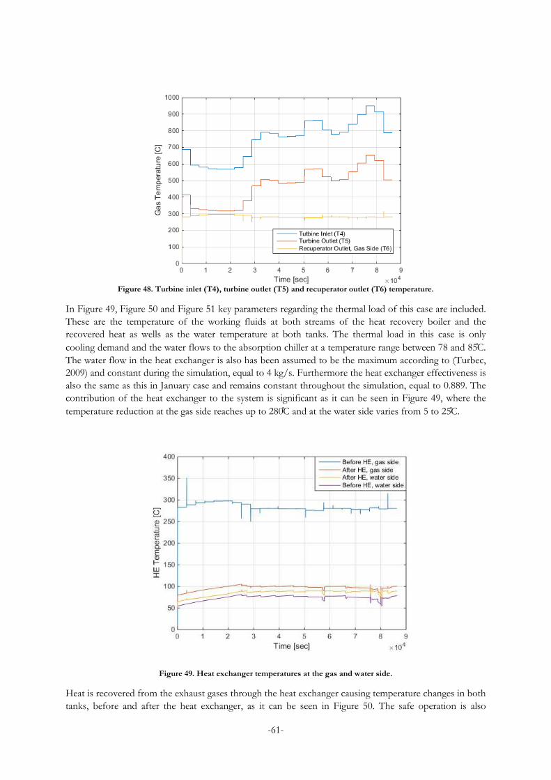
-61-
Figure 48. Turbine inlet (T4), turbine outlet (T5) and recuperator outlet (T6) temperature.
In Figure 49, Figure 50 and Figure 51 key parameters regarding the thermal load of this case are included.
These are the temperature of the working fluids at both streams of the heat recovery boiler and the
recovered heat as wells as the water temperature at both tanks. The thermal load in this case is only
cooling demand and the water flows to the absorption chiller at a temperature range between 78 and 85C.
The water flow in the heat exchanger is also has been assumed to be the maximum according to (Turbec,
2009) and constant during the simulation, equal to 4 kg/s. Furthermore the heat exchanger effectiveness is
also the same as this in January case and remains constant throughout the simulation, equal to 0.889. The
contribution of the heat exchanger to the system is significant as it can be seen in Figure 49, where the
temperature reduction at the gas side reaches up to 280C and at the water side varies from 5 to 25C.
Figure 49. Heat exchanger temperatures at the gas and water side.
Heat is recovered from the exhaust gases through the heat exchanger causing temperature changes in both
tanks, before and after the heat exchanger, as it can be seen in Figure 50. The safe operation is also

-62-
ensured by the two valves handling in a way that prevents the water vaporization at the water side. The
purpose of both valves and the set point of the water temperature after the heat exchanger are the same as
the January case and adjusted at 90C. As far as the water tanks are referred regarding the temperature, the
water flows to the absorption chiller at temperature from 78 to 85 C while the water temperature in Tank
2 starts from 10C and after the first 26 000 sec of the simulation increases. At this point, the water
temperature after the heat exchanger tends to become higher than 90C so the valves open, allowing hot
water to flow to Tank 2 and reach temperatures up to 72 C.
Figure 50. Water temperatures in the tanks, before the heat exchanger and after the heat exchanger.
The case of August was selected due to its cooling demand which is the highest of the year. As it can be
seen in Figure 51, this polygeneration system is investigated and unlike the January case, no additional heat
from any auxiliary system is required in order to cover the thermal load in the case of August. In this case
the thermal load is much lower than the case of January case and it is estimated to be about 1 130 kWh.
Consequently no additional fuel is consumed by the auxiliary boiler while the total fuel consumption of
each household is 221.8 kg/day. The total fuel consumption is lower than the case of January however it is
not that much lower since the electricity demand is higher.

-63-
Figure 51. Recovered heat by the heat exchanger and additional supplied het by the auxiliary boiler.

-64-
7 Conclusions and future work
In this thesis a polygeneration system is modeled and the operation of the system during two different
days of the year (one day in January and one day in August) has been investigated and analyzed. The
components of this polygeneration system were predetermined and the challenges in this work are the
proper configuration of them and an operational strategy which would ensure an efficient and safe
operation. More specifically the system consists of a microturbine, a heat storage system, a heat exchanger
as heat recovery boiler and an absorption chiller. The main purpose of this study is the modeling of a
polygeneration system in Matlab/Simulink, aiming to understand better the behavior of the system, with
special focus on the microturbine modeling. The usage of microturbines in such systems is getting more
attractive due to their fuel flexibility however their modeling is of high significance because of their
complexity. Special focus is also given to the microturbine data due to their confidential character and the
lack of experimental data for the specific microturbine model which is the Turbec T-100.
Nowadays most of the gas turbine models in Matlab/Simulink are based on Rowen’s model nonetheless
none of them is explained and analyzed in order to be applied for a microturbine. For this reason the
microturbine is analyzed thermodynamically and the model is developed according to this analysis. As far
as the control of the system is concerned, this is based on a previous work but modified according to the
microturbine’s data. The model is a useful tool for the system analysis and the energy monitoring of the
system as well as it can ensure an effective operation. Furthermore the model cannot be applied for
different cases if no modification of the system has initially been implemented. First of all the ambient
temperature should be modified properly and the appropriate electric and thermal load should be inserted.
The system is provided with no electricity storage, therefore the highest electricity demand throughout the
model simulation should not exceed 100 kWe which is the rated power of Turbec T-100. Accordingly the
first priority of the system from the energy supply point of view is the electricity so the microturbine
follows the electricity demand and the resulted produced heat from the electricity generation is available
for thermal load supply. Therefore the challenge in this system is the control of the temperature in order
to prevent vaporization in the water pipes and the storage tanks. There are two alternatives in order to
confront the aforementioned challenge; the first is to control the water mass flow at the heat recovery
boiler and the second is the implementation of two valves in the system. The first alternative could ensure
the operation of the system, maintaining the desired water temperatures in the system, while on the other
hand this principle could have as a result the increase of the wasted heat to the environment. The water
temperature depends on the water mass flow which enters the heat recovery boiler so the higher water
mass flow which enters the heat recovery boiler, the less useful heat is dumped to the environment. In this
work the second alternative is implemented and the water mass flow is adjusted to the highest possible
value and kept constant at 4 kg/s in order to absorb as much heat as possible. The utilization of the valves
in the system as well as the usage of the secondary tank is some of the key components of the system. The
water temperature is adjusted by these two valves and the absorbed useful heat is distributed to both tanks
appropriately, aiming to maintain the desired water temperatures throughout the system. To summarize,
the user should insert the ambient temperature, the load curves and the lower heating value of the fuel as
well as to modify the valves in order to run the simulation. The valves can be modified during the
simulation and the used values can be stored and transferred to a signal builder block.
The conclusions can be separated into two categories; the first is regarding the validation process and the
second category regarding the investigation of the two different cases as they are mentioned in The case
study section. As far as the model is concerned regarding the validation process of the microturbine
model, the model is developed by considering simulation results of a previous research work. For this
reason the mentioned data and results can perform deviations, comparing to a real life machine. On the
other hand, the comparison between the results of the test simulation with the applied data showed the
high accuracy of the model with small divergences up to 2.1%. As it can be seen in the validation section,
the model could be considered as a reliable Simulink model however the model’s behavior should be
studied with PID controllers instead of lead lag transfer function. The usage of a PID controller should
-65-
not perform variations from the final results however the control of the system can be less complicated.
Last but not least from the model validation, it is concluded that Turbec T-100 is more efficient when it
operates between 80% and 90% of the rated produced electricity. Regarding the results, the two selected
cases correspond to the maximum heating (January) and cooling (August) demand respectively. From the
results, it can be noticed that the produced thermal energy, in the case of January, is not enough so the
usage of an auxiliary boiler is needed. On the other hand as far as the case of August is concerned
regarding the cooling demand, the cooling demand can be fully supplied by the system. Furthermore the
hot water in the secondary tank reaches temperatures higher than 55 C for a long period which is
something that is should be investigated in order this amount of thermal energy to be exploited by other
applications for further purposes.
Last but not least, a future work would be necessary in order to provide useful results and comparisons,
some aspects that could be investigated are the following:
• The usage of an externally fired micro gas turbine as component of this polygeneration system.
• The usage of electricity storage.
• Investigation of the lithium-bromide refrigerating machine as component of this polygeneration
system instead of the absorption chiller as it is implemented in Polycity project Ostfildern,
Germany.
• The development of a model with PID controllers.
• One part of the natural gas consumption could be substituted by the municipal solid waste of
these households and the investigation of the economic feasibility.

-66-
Bibliography
Angrisani, G., Rosato, a., Roselli, C., Sasso, M., & Sibilio, S. (2012). Experimental results of a micro-
trigeneration installation. Applied Thermal Engineering, 38, 78–90.
doi:10.1016/j.applthermaleng.2012.01.018
Bank Tavakoli, M. R., Vahidi, B., & Gawlik, W. (2009). An educational guide to extract the parameters of
heavy duty gas turbines model in dynamic studies based on operational data. IEEE Transactions on
Power Systems, 24(3), 1366–1374. doi:10.1109/TPWRS.2009.2021231
Bianchi, M., Pascale, A. De, Melino, F., & Peretto, A. (2014). Performance prediction of micro-CHP
systems using simple virtual operating cycles, 71.
Camporeale, S. M., Fortunato, B., Torresi, M., Turi, F., Meccanica, D., Dmmm, M., … Bari, V. A. a.
(2014). Part load performance and operating strategies of a natural gas-biomass dual fuelled
microturbine for CHP generation, 1–15.
Chan, T., Kong, H., Lai, L. L., & Sciences, M. (2014). Permanent Magnet Machines for Distributed Generation :
A Review Introduction generator ( PMSG ) Radial-flux PMSG for isolated operation Linear PMSG Axial-flux
PMSG. Hong Kong, China.
Chapman, S. J. (2005). Electric Machinaery Fundamentals, 746.
Chu, S., & Majumdar, A. (2012). Opportunities and challenges for a sustainable energy future. Nature,
488(7411), 294–303. doi:10.1038/nature11475
City of Sydney. (2015). Sydney Town Hall House trigeneration. Sydney, Australia. Retrieved from
http://www.cityofsydney.nsw.gov.au/vision/towards-2030/sustainability/carbon-
reduction/trigeneration
Compower. (2015). Compower.
Concerto Programme. (2015a). POLYCITY Innovation: Energy and environmental concepts of the POLYCITY
project in Cerdanyola del Vallès. Barcelona, Spain.
Concerto Programme. (2015b). POLYCITY project. Retrieved from
http://www.polycity.net/en/index.html
Concerto Programme. (2015c). POLYCITY Project: Energetic and Urban Regeneration of the Arquata District in
the city of Torino. Turin, Italy.
Concerto Programme. (2015d). POLYCITY Technique: Energy concepts in the POLYCITY project
Scharnhauser Park. Ostfildern, Germany.
Elkington, K. (2014). Power Generator Technologies for Wind Turbine Applications. Stockholm: Svenska
Kraftnät.
Elsied, M. F., Oukaour, A., Gualous, H., Slamani, Y., Hassan, R., & Amin, A. (2014). Modeling , Control
and Optimization of a Small Scale CHP System in Island operating Mode based on Fuzzy logic
controller Key words, (12).

-67-
Farret, F., & Simoes, G. (n.d.). Integration of alternative sources of energy. New Jersey: John Wiley & Sons Inc.
Geoclima Smart HVAC Solutions. (2013). Pulkovo, Enrgy Center. Retrieved from
http://www.geoclima.com/portfolio-item/pulkovo-energy-center/
Goldstein, L., Hedman, B., Knowles, D., Freedman, S. I., & Woods, R. (2003). Gas-Fired Distributed
Energy Resource Technology Characterizations. Energy, 226. doi:10.2172/15005819
Guda, S. R. (2005). Modelling and powe management of a hybrid wind-microturbine power generation system. Montana
State University.
Hansen, U., & Kautz, M. (2005). The Externally Fired Gas Turbine (EFGT-Cycle) and Simulation of the
Key Components. Retrieved from http://coal2nuclear.com/MSR - Externally Fired Gas
Combustion Turbine.pdf
Haugwitz, S. (2003). Modelling of microturbine systems, (May). Retrieved from
http://www.nt.ntnu.no/users/skoge/prost/proceedings/ecc03/pdfs/209.pdf
Hugé, J., Waas, T., Eggermont, G., & Verbruggen, A. (2011). Impact assessment for a sustainable energy
future-Reflections and practical experiences. Energy Policy, 39(10), 6243–6253.
doi:10.1016/j.enpol.2011.07.023
IEEE Spectrum. (2014). Groundbreaking Smart Polygeneration Microgrid Project: University Campus of
Savona, Italy. Retrieved from http://spectrum.ieee.org/webinar/groundbreaking-smart-
polygeneration-microgrid-project-university-campus-of-savona-italy
Kallio, S. (2012). Modelling of a combined heat and power system. Tampereen Teknillinen Yliopisto.
Kärkkäinen, S. (2011). Heat pumps for cooling and heating, Task XVII: Integration of Demand Side Management,
Distributed Generation, Renewable Energy Sources and Energy Storages. Helsinki.
Kozman, T. A., Kaur, B., & Lee, J. (2009). Design of Heat Exchanger for Heat Recovery in CHP Systems.
KTH Polygeneration Lab. (2015). Explore polygeneration. Retrieved from http://www.explore-
polygen.com/the_project/
KTH Royal Institute of Technology. (2013). Sustainable Power Generation cource MJ2405: Equations,
diagrams, tables help file, 1–29.
Kumar, A., Sandhu, K., Jain, S., & Kumar, P. S. (2009). Modeling and Control of Micro-Turbine Based
Distributed Generation System. International Journal of Circuits, Systems and Signal Processing, 3(2), 65–72.
Retrieved from http://www.naun.org/journals/circuitssystemssignal/cssp-100.pdf
Lipp, J. (2012). Field test with Stirling engine micro-combined heat and power units in residential
buildings. Proceedings of the Institution of Mechanical Engineers, Part A: Journal of Power and Energy, 227(1),
43–52. doi:10.1177/0957650912458755
Martin, V. (2014). Introduction to thermal energy storage. Dept of Energy Technology, KTH Royal Institute of
Technology. Stockholm, Sweden. Retrieved from \\Kwi-
server\literatur\edo\articles\DSH\DSH_0458.pdf\n\\Kwi-
server\literatur\edo\articles_ocrtxt\DSH\DSH_0458.txt

-68-
McQuiston, F. C., & Parker, J. D. (1999). Heating, Ventilation and Air Conditionning, Analysis and Design. (M.
Vrachopoulos, Ed.) (1st Greek.). Oklahoma: John Wiley & Sons Inc.
Murty, D. M. S. R. (2014). Modeling of Gas Turbine and Its Control System.
Ortiga, J., Bruno, J. C., Coronas, A., & Grossman, I. E. (2007). Review of optimization models for the
design of polygeneration systems in district heating and cooling networks, 24, 1–6.
doi:10.1016/S1570-7946(07)80211-2
Pantaleo, A. M., Camporeale, S. M., & Shah, N. (2013). Thermo-economic assessment of externally fired
micro-gas turbine fired by natural gas and biomass: Applications in Italy. Energy Conversion and
Management, 75, 202–213. doi:10.1016/j.enconman.2013.06.017
Rohatgi, A. (2015). WebPlotDigitizer. Retrieved from http://arohatgi.info/WebPlotDigitizer/app/?
Rowen, W. I. (1983). Simplified Mathematical Representations of Heavy-Duty Gas Turbines. Journal of
Engineering for Power, 105(4), 865. doi:10.1115/1.3227494
Salomón, M. (2013). Renewable Energy Technology: Introduction to Renewable Energy Technology. In
Master Sustainable Energy Engineering at KTH Royal Institute of Technology (pp. 1–135). Stockholm.
Shah, R. K., & Sekulic, D. P. (2006). Heat Exchangers for Fuel Cell and Hybrid System Applications. Journal of
Fuel Cell Science and Technology (Vol. 20). doi:10.1115/1.2173665
Single Electricity Market Operator. (2015). Modelling and Analysis: Market Modelling. Retrieved from
http://www.sem-o.com/MarketDevelopment/Pages/Modelling and Analysis.aspx
Skagestad, B., & Mildenstein, P. (2002). District Heating and Cooling Connection Handbook - Programme of
Research, Development and Demonstration on District Heating and Cooling. Retrieved from
http://dedc.dk/sites/default/files/programme_of_research_development_and_demonstration_on_
district_heating_and_cooling.pdf
Soares, C. P. E. (2007). Microturbines: Applications for Distributed Energy Systems.
Southern California Gas Company New Buildings Institute. (1998). Absorption Chillers. Advanced Design
Guideline Series.
Stine, W. B., & Geyer, M. (2001). Power Cycles for Electricity Generation. In Power from the Sun. Retrieved
from http://www.powerfromthesun.net/Book/chapter12/chapter12.html
Tomlinson, J. (1992). Thermal energy storage. Technical Progress Report, Apr. 1990-Mar. …, 1–27.
doi:10.1080/00908310151134004
Traverso, A., Massardo, A. F., & Scarpellini, R. (2006). Externally Fired micro-Gas Turbine: Modelling
and experimental performance. Applied Thermal Engineering, 26(16), 1935–1941.
doi:10.1016/j.applthermaleng.2006.01.013
Turbec. (2009). Technical Description T100 Natural gas. T100 Microturbine System.
Ulloa, C., Míguez, J. L., Porteiro, J., Eguía, P., & Cacabelos, A. (2013). Development of a transient model
of a stirling-based CHP system. Energies, 6, 3115–3133. doi:10.3390/en6073115

-69-
University of Michigan. (2015). Control Tutorieal for Matlab Simulink. Retrieved from
http://ctms.engin.umich.edu/CTMS/index.php?example=Introduction§ion=SimulinkModelin
g
Velez, V. (2010). Design of a Control Strategy for Optimal Operation of an Autonomous Distributed Generation System
for Electricity and Heat. Applied Sciences. Delft University of Technology.
Zimmermann, J.-P., Evans, M., Lineham, T., Griggs, J., Surveys, G., Harding, L., … Roberts, P. (2012).
Household Electricity Survey A study of domestic electrical product usage. Intertek.
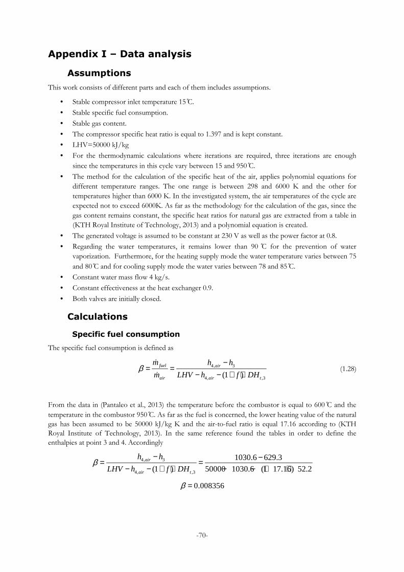
-70-
Appendix I – Data analysis
Assumptions
This work consists of different parts and each of them includes assumptions.
• Stable compressor inlet temperature 15 C.
• Stable specific fuel consumption.
• Stable gas content.
• The compressor specific heat ratio is equal to 1.397 and is kept constant.
• LHV=50000 kJ/kg
• For the thermodynamic calculations where iterations are required, three iterations are enough
since the temperatures in this cycle vary between 15 and 950 C.
• The method for the calculation of the specific heat of the air, applies polynomial equations for
different temperature ranges. The one range is between 298 and 6000 K and the other for
temperatures higher than 6000 K. In the investigated system, the air temperatures of the cycle are
expected not to exceed 6000K. As far as the methodology for the calculation of the gas, since the
gas content remains constant, the specific heat ratios for natural gas are extracted from a table in
(KTH Royal Institute of Technology, 2013) and a polynomial equation is created.
• The generated voltage is assumed to be constant at 230 V as well as the power factor at 0.8.
• Regarding the water temperatures, it remains lower than 90 C for the prevention of water
vaporization. Furthermore, for the heating supply mode the water temperature varies between 75
and 80 C and for cooling supply mode the water varies between 78 and 85 C.
• Constant water mass flow 4 kg/s.
• Constant effectiveness at the heat exchanger 0.9.
• Both valves are initially closed.
Calculations
Specific fuel consumption
The specific fuel consumption is defined as
4, 3
4, ,3(1 )fuel air
air air t
m h h
m LHV h f DHβ
−= =
− − + ⋅ɺ
ɺ (1.28)
From the data in (Pantaleo et al., 2013) the temperature before the combustor is equal to 600 C and the
temperature in the combustor 950 C. As far as the fuel is concerned, the lower heating value of the natural
gas has been assumed to be 50000 kJ/kg K and the air-to-fuel ratio is equal 17.16 according to (KTH
Royal Institute of Technology, 2013). In the same reference found the tables in order to define the
enthalpies at point 3 and 4. Accordingly
4, 3
4, ,3
1030.6 629.3
(1 ) 50000 1030.6 (1 17.16) 52.2air
air t
h h
LHV h f DHβ
− −= =− − + ⋅ − − + ⋅
0.008356β =
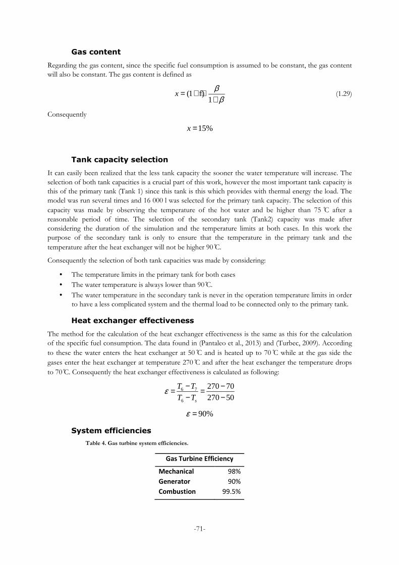
-71-
Gas content
Regarding the gas content, since the specific fuel consumption is assumed to be constant, the gas content
will also be constant. The gas content is defined as
(1 f)1
xβ
β= + ⋅
+ (1.29)
Consequently
15%x =
Tank capacity selection
It can easily been realized that the less tank capacity the sooner the water temperature will increase. The
selection of both tank capacities is a crucial part of this work, however the most important tank capacity is
this of the primary tank (Tank 1) since this tank is this which provides with thermal energy the load. The
model was run several times and 16 000 l was selected for the primary tank capacity. The selection of this
capacity was made by observing the temperature of the hot water and be higher than 75 C after a
reasonable period of time. The selection of the secondary tank (Tank2) capacity was made after
considering the duration of the simulation and the temperature limits at both cases. In this work the
purpose of the secondary tank is only to ensure that the temperature in the primary tank and the
temperature after the heat exchanger will not be higher 90 C.
Consequently the selection of both tank capacities was made by considering:
• The temperature limits in the primary tank for both cases
• The water temperature is always lower than 90 C.
• The water temperature in the secondary tank is never in the operation temperature limits in order
to have a less complicated system and the thermal load to be connected only to the primary tank.
Heat exchanger effectiveness
The method for the calculation of the heat exchanger effectiveness is the same as this for the calculation
of the specific fuel consumption. The data found in (Pantaleo et al., 2013) and (Turbec, 2009). According
to these the water enters the heat exchanger at 50 C and is heated up to 70 C while at the gas side the
gases enter the heat exchanger at temperature 270 C and after the heat exchanger the temperature drops
to 70 C. Consequently the heat exchanger effectiveness is calculated as following:
6 7
6
270 70
270 50s
T T
T Tε − −= =
− −
90%ε =
System efficiencies
Table 4. Gas turbine system efficiencies.
Gas Turbine Efficiency
Mechanical 98%
Generator 90%
Combustion 99.5%

-72-
Appendix II – System modeling
Table 5. Model input parameters.
Parameter Symbol Value
Fuel system constant c 1
Governor lead time constant [s] C1 0.4
Governor lag time constant [s] C2 3
Radiation shield time constant [s] C3 15
Thermocouple shield time constant [s] C4 2.5
Temperature controller time constant [s] C5 3.3
Coefficient of performance COP 0.65
Governor Gain K 25
No load consumption factor k_NL 0.26
Fuel system actuator gain Kf 1
Valve position gain Kv 1
Turbine smoothness coefficient SM 0.3005
Turbine smoothness coefficient 1 SM1 1
Compressor discharge time lag [s] TCD 0.2
Combustion reaction transport delay [s] TCR 0.01
Fuel system actuator time constant [s] Tf 0.04
Temperature controller integration constant [ C] Tt 233
Turbine exhaust transport delay [s] TTD 0.04
Valve position time constant [s] Tv 0.005
Speed control system constant z 1
Rated exhaust temperature [ C] Texh_Ref 650

Figure 52. Load, generator and microturbine

-74-
Figure 53. Heat exchanger and heat storage

-75-
Figure 54. Mictoturbine
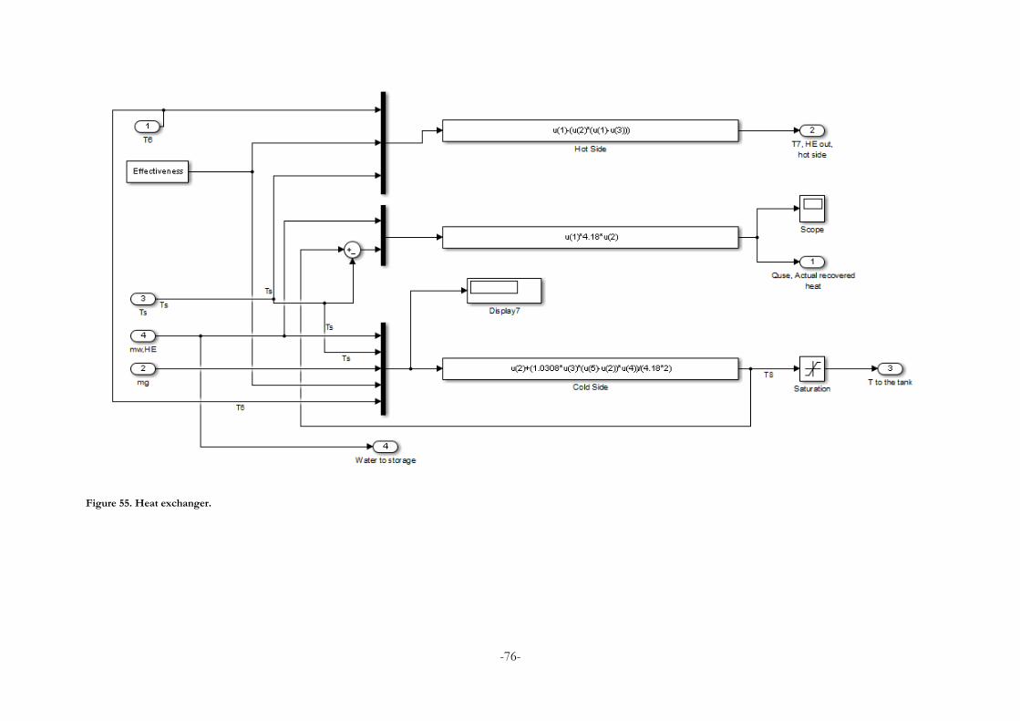
-76-
Figure 55. Heat exchanger.

-77-
Figure 56. Primary tank
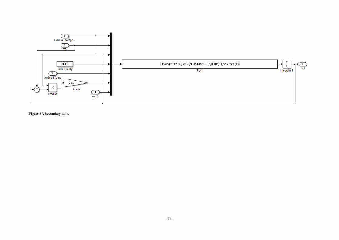
-78-
Figure 57. Secondary tank.

Appendix III – Case study
As far as the case study is concerned the CASAnova software is implemented, the results of it was that the
total heating demand in January is about 1 338 kWh and the cooling demand is 357 kWh in August. Both
amounts of energy were divided by the days of each month respectively in order to define the amount of
energy that is required in order to supply the thermal load of the system. Consequently it was found that
43.2 kWh/day and 11.9 kWh/day are required for the heating demand in January and the cooling demand
in August respectively. Afterwards both amounts of thermal energy were distributed properly in the
following normalized load curves in Figure 32 and Figure 33.


