See discussions, stats, and author profiles for this publication at: https://www.researchgate.net/publication/316991276 Modeling and Simulation of Automatic Generation Control System for Synchronous Generator with Model Predictive Co.... Article · January 2016 CITATIONS 0 READS 59 3 authors: Some of the authors of this publication are also working on these related projects: Modeling of AGC Systems for Synchronous Generator View project Boiler Modeling View project Muyiwa Michael Orosun University of Ilorin 12 PUBLICATIONS 3 CITATIONS SEE PROFILE Rapheal O. Orosun Bayero University, Kano 4 PUBLICATIONS 6 CITATIONS SEE PROFILE Sunusi Sani Adamu Bayero University, Kano 15 PUBLICATIONS 66 CITATIONS SEE PROFILE All content following this page was uploaded by Muyiwa Michael Orosun on 17 May 2017. The user has requested enhancement of the downloaded file.
In this study, automatic generation control system was used to control the real and reactive power of a power system in order to keep the system in the steady state. Firstly, the load frequency control (LFC) loop and automatic voltage regulator loop (AVR) were isolated and then studied separately. Secondly, the combined load frequency control loop (LFC) and automatic voltage regulator loop (AVR) was studied. MATLAB-SIMULINK
® simulation software was used to examine the voltage and frequency changes due to
some specific load variation. Worth noting however is the use of Neural Network Controller—Model Predictive Controller (MPC)——to obtain the system dynamic response. Lastly, the response obtained using MPC controller was compared with that obtained using conventional PID controller from earlier work. Significant improvements were observed in the overshoot/undershoot and settling time of the power system indicating the potential advantages of Model Predictive Controller over conventional PID controller.
Key Words: Model Predictive Controller MPC, Automatic Voltage Regulator, Automatic
Generation Control, Load Frequency Control, PID Controller.
Received:08.08.2016 Accepted: 11.11.2016.
1. INTRODUCTION
The automatic generation control consist of two main loops: load frequency control (LFC) loop and automatic voltage regulator (AVR) loop. The LFC loop controls the real power and frequency, while the AVR loop regulates the reactive power and voltage magnitude, where the main purpose of these controllers is to maintain the frequency and voltage within permissible limits. Hence, the study of automatic generation control is required in the operation of interconnected power system (Vikas et al., 2014; Anbarasi et al., 2014; Ahmad et al., 2013; Umashankar, 2010; Soe, 2009; Wang, 2003).
Automatic Generation Control (AGC) is a feedback control system that regulates the power output of electric generators to maintain a specified system frequency and scheduled interchange. In practice, AGC of a power system is a set of equipment and computer programs that applies closed loop
feedback control to regulate the power system frequency to a scheduled value, to maintain all scheduled power transactions to the contract value, as well as the net power interchange at the value required by the interchange contracts, and to maintain each generation units operation at the most economic value (economic dispatch) (Lakshmi et al., 2016; Karnavas and Dedousis, 2010; Farook et al., 2012).
This paper uses model predictive control MPC and conventional PID control method to control load frequency control loop (LFC) and automatic voltage regulator loop (AVR) of the synchronous generator. Simulation studies were made to determine the degree of improvement that could be gained in AGC dynamic response by the application of MPC controller as compared with the conventional PID controller.
Firstly, the load frequency control (LFC) loop and automatic voltage regulator loop (AVR) were isolated and then studied
separately. Secondly, the combined load frequency control loop (LFC) and automatic voltage regulator loop (AVR) was studied. MATLAB-SIMULINK® simulation software was used to examine the voltage and frequency changes due to some specific load variation. Further simulation studies were carried out using Model Predictive Controller (MPC) to obtain the system dynamic response. Lastly, the response obtained using MPC controller was compared with that obtained using conventional PID controller from earlier work. Finally, summary, conclusion and recommendations were made.
The PID controllers are commonly used in AGC of power systems (Lakshmi et al., 2016; Kanavas an dedousis, 2010; Anant et al., 2008). The essential selection criteria of a controller are its proper control performance, maximum speed and its robustness towards the nonlinearity, time varying dynamics, disturbances and other factors. The PID controller has been recommended as a reputed controller in this accord and it also can be used for higher order systems (Lukman and Nuradeen, 2015; Anbarasi et al., 2014; Orosun and Adamu, 2012). The Ziegler Nichols (ZN) classic tuning method is normally used to predict the gain parameters of PID controller. But these types of fixed gain controllers are designed for nominal operating conditions and they cannot provide a proper control action over a wide range of operating conditions. The adaptability of such controllers on the varying load demand and uncertainties are also difficult and thereby quite often impractical for implementation. In response to these challenges so many intelligent approaches have been introduced for optimal tuning of controllers in AGC (Anant et al, 2008). In this paper, Model Predictive Control (MPC) was implemented for optimal control in a single area power system AGC. The adequacy of the proposed MPC controller was confirmed by comparing the
results with the conventionally tuned ZN-PID controller.
The idea of model predictive control (MPC) was first investigated in the 1980s (Orosun and Adamu, 2013). MPC was intended to offer a new adaptive control alternative. Clark et al in 1987 showed that the receding-horizon method depends on predicting the plant’s output several steps ahead based on assumptions about future control actions. An assumption that was made was that, there is a ‘control horizon’ beyond which all control increments become zero. MPC has proved to be an effective strategy in many fields of applications (Orosun and Adamu, 2013; Qingxiang and Richard, 2013), with good temporal and frequency properties such as small overshoot, cancellation of disturbances, good stability and robustness margins. This paper presents a model predictive control for a single area power system AGC.
1.1 Aim and Objectives
This work is aimed at developing a simulation model of an Automation Generation Control AGC. The objectives of the work include;
To develop and study separately the simulation model of Load Frequency Control LFC.
To develop and study separately the simulation model of Automatic Voltage Regulator AVR.
To study the combined LFC loop and AVR loop noting the effect on MPC controller due to the combination of LFC and AVR loops.
Compare the results obtained using MPC controller with the results obtained in earlier work using conventional PID controller.
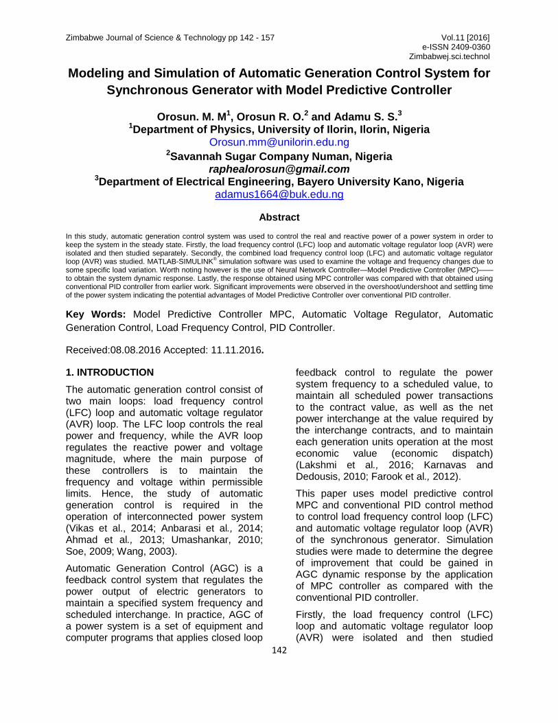
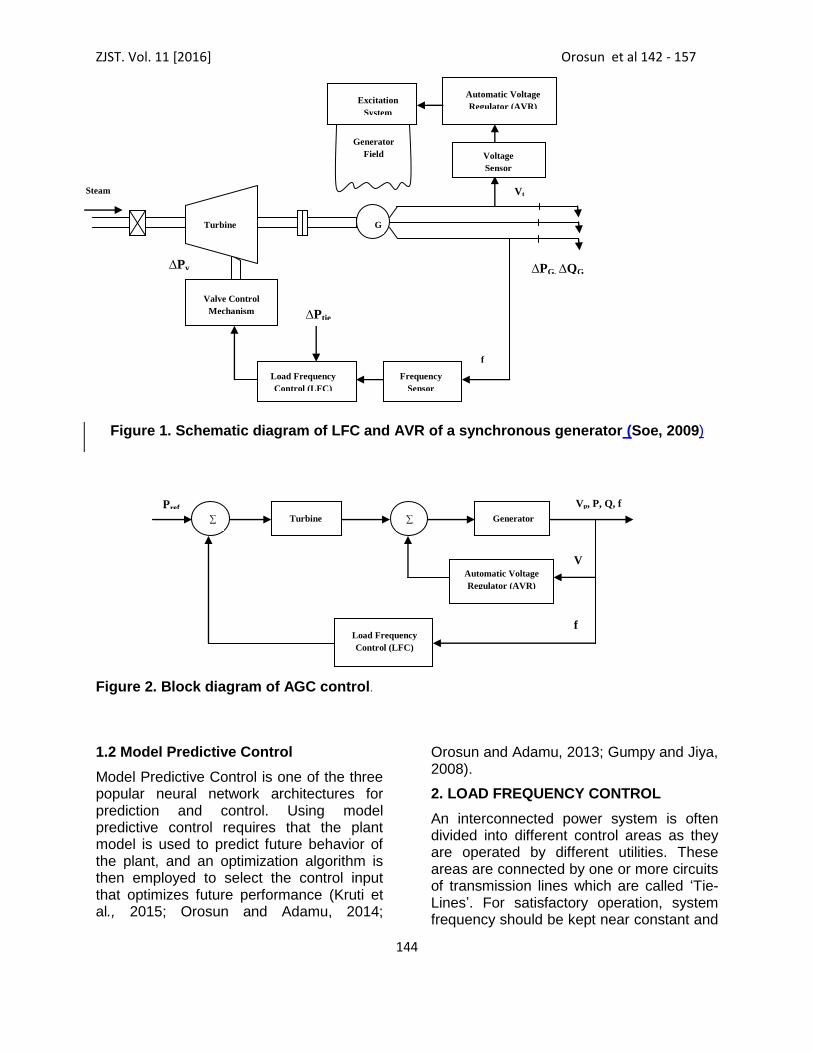
The basic components of the AGC are expressed in Figure 1 and Figure 2 with schematic and block diagram respectively.
ZJST. Vol. 11 [2016] Orosun et al 142 - 157
144
Figure 1. Schematic diagram of LFC and AVR of a synchronous generator (Soe, 2009)
Figure 2. Block diagram of AGC control.
1.2 Model Predictive Control
Model Predictive Control is one of the three popular neural network architectures for prediction and control. Using model predictive control requires that the plant model is used to predict future behavior of the plant, and an optimization algorithm is then employed to select the control input that optimizes future performance (Kruti et al., 2015; Orosun and Adamu, 2014;
Orosun and Adamu, 2013; Gumpy and Jiya, 2008).
2. LOAD FREQUENCY CONTROL
An interconnected power system is often divided into different control areas as they are operated by different utilities. These areas are connected by one or more circuits of transmission lines which are called ‘Tie-Lines’. For satisfactory operation, system frequency should be kept near constant and
Generator
Field
Valve Control
Mechanism
Load Frequency
Control (LFC)
f
Frequency
Sensor
∆Ptie
G Turbine
Excitation
System
Voltage
Sensor
Automatic Voltage
Regulator (AVR)
Vt Steam
∆PG, ∆QG
∆Pv
Load Frequency
Control (LFC)
f
Turbine ∑ Generator
Pref
∑
Vp, P, Q, f
V Automatic Voltage
Regulator (AVR)
ZJST. Vol. 11 [2016] Orosun et al 142 - 157
145
power flow between different areas should be controlled as scheduled despite the variation of load in different areas. This function of AGC is commonly referred to Load Frequency Control LFC (Farook et al., 2011; Oguz, 2011; Navreet, 2008). The operation objectives of the LFC controller are to maintain reasonably uniform frequency, to divide the load between generators, and to control the tie-line interchange schedules [1]. The change in frequency and tie-line real power are sensed, which is a measure of the change in rotor angle δ, i.e. the error ∆δ to be corrected. The error signal, i.e. ∆f and ∆Ptie
are amplified, mixed, and transformed into a real power command signal ∆Pv, which is sent to the prime mover, therefore, brings change in the generator output by an amount ∆Pg which will change the values of ∆f and ∆Ptie within the specific tolerance (Anbarasi et al., 2014; Vikas et al., 2014; Zong et al., 2014; Farook, 2011).
2.1 Modeling of Load Frequency Control (LFC) Loop
It is assumed that first order transfer function is able to capture the dynamics of the individual components of the LFC loop. This linear model takes care of the major time constants and neglects the saturation and other nonlinearities for the simplicity in analysis. In modeling the LFC, it is needed to present linearized mathematical formulas of the generator, load, prime mover, and governor to simulate LFC loop (Kundur, 1994)
2.1.1 Governor Model
The governor acts as a comparator whose output ∆Pref and the power ∆f/R (Vikas et al., 2014 ; Zong et al., 2014; Soe, 2009; Kundur, 1994).
)(1
)()( sFR
sPsP refg
)1(
2.1.2 Hydraulic Valve Actuator Model
Hydraulic valve actuator controls the steam flow into the turbine. Hydraulic valve actuator relates the speed governor output ∆Pg and turbine input or hydraulic valve actuator output ∆Pv (Vikas et al., 2014 ; Zong et al., 2014; Soe, 2009; Kundur, 1994).
)(1
1)( sP
ssP g
g
v
)2(
2.1.3 Prime Mover Model
The prime mover or turbine, whose input is the position output of hydraulic valve, ∆Pv, drives the generator. The simplest prime mover model for the non-reheat steam turbine can be approximated with a single time constant λT (Vikas et al., 2014; Zong et al., 2014; Soe, 2009; Kundur, 1994).
ssP
sPsG
Tv
mT
1
1
)(
)()(
)3(
2.1.4 Generator Model
By solving the following swing equation of a synchronous machine (Vikas et al., 2014; Zong et al., 2014; Soe, 2009; Kundur, 1994)
Dm
s
PPdt
dH
2
22
)4(
The linearized generator model can be approximated as follow (Vikas et al., 2014; Zong et al., 2014; Soe, 2009; Kundur, 1994):
)()(2
1)( sPsP
HssF Dm
)5(
2.1.5 Load Model
The load on a power system can be divided in two types: resistive load and frequency sensitive load. Therefore, the composite load on power system can be represented by the following equation (Vikas et al., 2014;
ZJST. Vol. 11 [2016] Orosun et al 142 - 157
146
Zong et al., 2014; Soe, 2009; Kundur, 1994)].
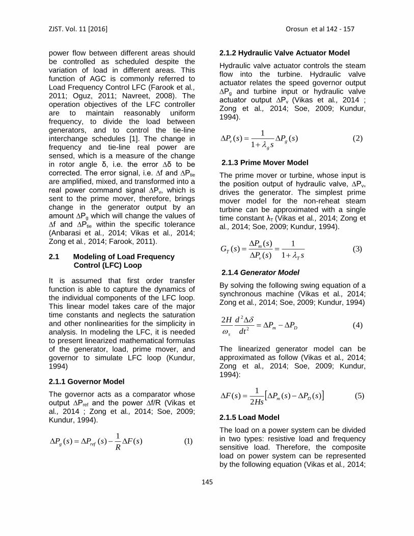
)()()( sDsPsP LD )6(
By combining the above equation, load frequency control can be represented by the following block diagram.
Figure 3. Block diagram for LFC control
2.1.6 Simulation of Load Frequency Control (LFC) Loop
The main specifications of any control system are: the control loop must have a sufficient degree of stability, acceptable transient frequency error response and zero steady state frequency error.
If the load on the system is increased, the turbine speed drops before the governor
can adjust the input of the steam to the new load. To restore the speed an integrator is added (rest action).
The nominal system parameters of LFC investigated in this paper are similar to the parameters commonly quoted in most of the research papers (Vikas et al, 2014 ; Zong et al, 2014; Soe, 2009; Kundur, 1994). They are given in Table 1.
Table 1. Values of the constants required for LFC loop
Parameter D H λg λT
Values 0.8 10 0.2 0.5
By combining the blocks in Figure 3, and adding the integrator (delay) to the blocks, the simulation diagram of the LFC loop can be represented in Figure 4 as follow:
- ∆Pref(s)
R
1
DHs 2
1 sg1
1
sT1
1
∆Pg(s)
∆ω(s)
∆PL(s)
∆Pm(s) ∆PV(s)
+ + -
ZJST. Vol. 11 [2016] Orosun et al 142 - 157
147
Figure 4. Simulink diagram for LFC loop with integrator (Rest Action)
Figure 5. Simulated result for LFC loop
Table 2. Comparison of results for LFC loop
Case K1 Undershoot Settling Time Steady-State Error
1 0 0.0264 15 0.000
2 3 0.0728 30 0.000
3 10 0.0696 21 0.000
4 7 0.0708 12 0.000
ZJST. Vol. 11 [2016] Orosun et al 142 - 157
148
From Table 2, the best response of the LFC loop occurs when gain KI was 7. This implies that case 4 gives the best tradeoff between overshoot/undershoot and settling time. Case 4 of the LFC loop was simulated in Figure 5.
2.2 Automatic Voltage Regulator AVR
The generator excitation system maintains generator voltage and controls the reactive power flow. The automatic voltage regulator controls generator excitation to maintain the reactive power. The role of an (AVR) is to hold the terminal voltage magnitude of a synchronous generator at a specified level (Indranil et al., 2014; Zong et al., 2014; Soe, 2009; Saadat, 1999; Kundur, 1994).
An increase in the reactive power load of the generator is followed by a drop in the terminal voltage magnitude. The voltage magnitude is sensed through a potential transformer on one phase. This voltage is rectified and compared to a dc set point signal. The amplified error signal controls the exciter field and increases the exciter terminal voltage. Thus, the generator field current is increased, which results in an increase in the generated emf. The reactive power generation is increased to a new equilibrium, raising the terminal voltage to the desired value (Indranil et al., 2014; Zong et al., 2014; Soe, 2009; Saadat, 1999; Kundur, 1994).
2.2.1 Modeling of AVR
Also, in modeling the AVR loop it was assumed that first order transfer function is able to capture the dynamics of the individual components of the AVR loop. This linear model takes care of the major time constants and neglects the saturation and other nonlinearities for the simplicity in analysis (Indranil et al., 2013; Kundur, 1999). In modeling the AVR, it is needed to present linearized mathematical formulas of the amplifier, exciter, generator, and sensor.
2.2.1.1 Amplifier Model
The amplifier can be represented by the time constant λA and gain KA (Indranil et al,
2014; Zong et al, 2014; Soe, 2009; Kundur, 1994).
s
K
sV
sV
A
A
e
A
1)(
)(
)7(
2.2.1.2 Exciter Model
The linearized exciter model takes into account the major time constant and ignores the saturation or other nonlinearities. In the simplest form the transfer function of the exciter is (Indranil et al., 2014; Zong et al., 2014; Soe, 2009; Kundur, 1994):
s
K
sV
sV
E
E
A
E
1)(
)(
)8(
2.2.1.3 Generator Model
The linearized model transfer function relating the generator terminal voltage to its field voltage can be represented by a gain KG and a time constant λG as follow (Indranil et al., 2014; Zong et al., 2014; Soe, 2009; Kundur, 1994):
s
K
sV
sV
G
G
E
t
1)(
)(
)9(
2.2.1.4 Sensor Model
The voltage is sensed through a potential transformer and, in one form, it is rectified through a bridge rectifier. The sensor is modeled by a simple first order transfer function as follow (Indranil et al., 2014; Zong et al., 2014; Soe, 2009; Kundur, 1994):
s
K
sV
sV
R
R
t
R
1)(
)(
)10(
ZJST. Vol. 11 [2016] Orosun et al 142 - 157
149
2.2.1.5 Simulation of AVR
MPC controller was used to control the generator excitation system and improve the dynamic response as well as reduce or eliminate the steady-state error (Qingxiang and Richard, 2013; Orosun and Adamu, 2013; Morari and Lee, 1999; Oluwande and Boucher, 1999).
Assuming that the estimates of the plant states are available at time k. The model predictive control action at time k is obtained by solving the optimization problem (Orosun and Adamu, 2013; Qingxiang and Lee, 2013):
1
0 1
2
,1 11),(p
i
n
j
jj
y
ji
y
ikrkikywuJ
2
1 1
2
arg,
2
,
u un
j
n
j
etjtj
u
jij
u
ji ikukikuwkikuw
)11(
Where, the subscript ""
j denotes the
thj component of a vector. "" kik
denotes the value predicted for time ik based on the information available at time k. u, ∆u and y denotes input, input increment, and output respectively. ε is the slack variable. r(k) is the current sample of the output reference.
The nominal system parameters of AVR investigated in this paper are similar to the parameters commonly quoted in most of the research papers (Indranil et al., 2014; Zong et al., 2014; Soe, 2009; Kundur, 1994). They are given in Table 3.
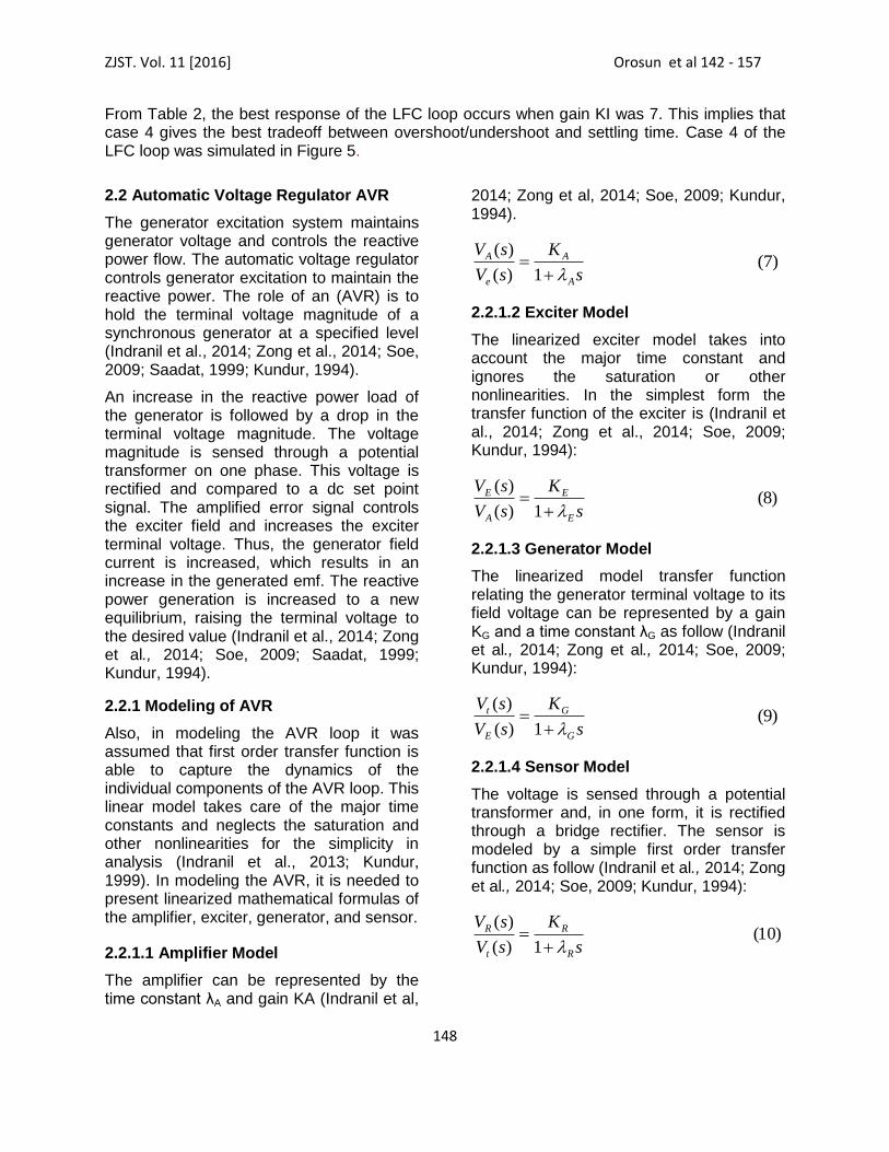
By adding MPC controller in forward path of AVR loop, the simulation diagram of the AVR with MPC controller can be represented as follow:
Step
1
0.05s+1
Sensor
Scope
MPC mv
mo
ref
MPC Controller
0.8
1.4s+1
Generator
1
0.4s+1
Exciter
10
0.1s+1
Amplifier
Figure 6. Simulink diagram for AVR loop with MPC
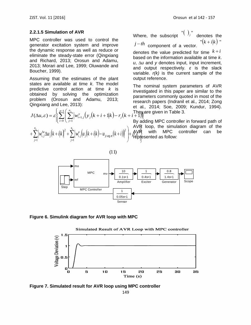
Figure 7. Simulated result for AVR loop using MPC controller
ZJST. Vol. 11 [2016] Orosun et al 142 - 157
150
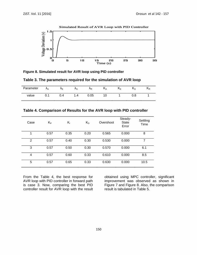
Figure 8. Simulated result for AVR loop using PID controller
Table 3. The parameters required for the simulation of AVR loop
Parameter λA λE λG λR KA KE KG KR
value 0.1 0.4 1.4 0.05 10 1 0.8 1
Table 4. Comparison of Results for the AVR loop with PID controller
Case KP KI KD Overshoot Steady-State Error
Settling Time
1 0.57 0.35 0.20 0.565 0.000 8
2 0.57 0.40 0.30 0.530 0.000 7
3 0.57 0.50 0.30 0.570 0.000 6.1
4 0.57 0.60 0.33 0.610 0.000 8.5
5 0.57 0.65 0.33 0.630 0.000 10.5
From the Table 4, the best response for AVR loop with PID controller in forward path is case 3. Now, comparing the best PID controller result for AVR loop with the result
obtained using MPC controller, significant improvement was observed as shown in Figure 7 and Figure 8. Also, the comparison result is tabulated in Table 5.
ZJST. Vol. 11 [2016] Orosun et al 142 - 157
151
Table 5. Comparison of Results for the AVR loop using MPC and PID controllers.
Controller Type
KP KI KD Overshoot Steady-State Error
Settling Time
PID Controller
0.57 0.50 0.30 0.240 0.000 7.8
MPC Controller
- - - 0.076 0.000 3.4
From Table 5, PID controller produced about 24% overshoot and settling time of 7.8 sec while the MPC controller produced less than 8% overshoot and settling time of 3.4sec.
3. COMBINED LFC AND AVR
Due to the weak coupling relationship between the LFC and AVR systems, the frequency and voltage were controlled separately. The coupling effects show as a small change in the electrical power ∆Pe, which is the product of the synchronizing power coefficient PS and the change in the power angle ∆δ. Taking into account the small effect of voltage on real power, the following linearized equation is obtained (Indranil et al, 2014; Zong et al, 2014; Soe, 2009; Kundur, 1994):
'
21 EKKPe
)12(
Where, K2 is the change in the electrical power for a change in the stator emf. Taking into account the small effect of rotor angle upon the generator terminal voltage is
(Zong et al, 2014; Soe, 2009; Kundur, 1994):
'
43 EKKVt
)13(
Where, K3 is the change in terminal voltage for a small change in rotor angle at constant stator emf, and K4 is the change in terminal voltage for a small change in the stator emf at constant rotor angle.
By modifying the generator field transfer function to include the effect of rotor angle δ, the stator emf is (Zong et al, 2014; Soe, 2009; Kundur, 1994):
)(1
5
'
KVs
KE t
G
G
)14(
3.1 Simulation of Combined LFC and AVR loop
By considering the combining effect discussed above and combining the LFC and AVR loops, the simulation diagram of the LFC and AVR loops can be represented as follow:
ZJST. Vol. 11 [2016] Orosun et al 142 - 157
152
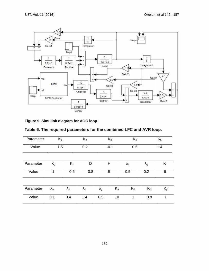
Figure 9. Simulink diagram for AGC loop
Table 6. The required parameters for the combined LFC and AVR loop.
Parameter K1 K2 K3 K4 K5
Value 1.5 0.2 -0.1 0.5 1.4
Parameter Kg KT D H λT λg KI
Value 1 0.5 0.8 5 0.5 0.2 6
Parameter λA λE λG λg KA KE KG Kg
Value 0.1 0.4 1.4 0.5 10 1 0.8 1
ZJST. Vol. 11 [2016] Orosun et al 142 - 157
153
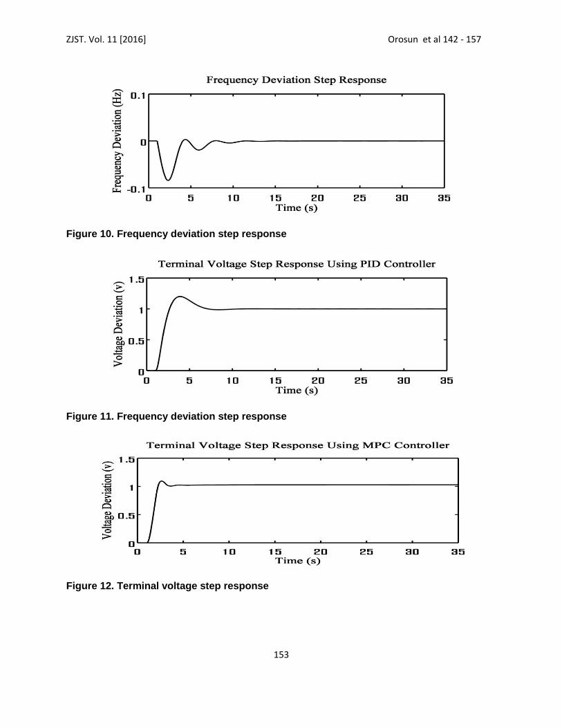
Figure 10. Frequency deviation step response
Figure 11. Frequency deviation step response
Figure 12. Terminal voltage step response
ZJST. Vol. 11 [2016] Orosun et al 142 - 157
154
Table 7. Comparison of Results for the AGC loop using MPC and PID controllers.
Controller Type
KP KI KD Overshoot Steady-State Error
Settling Time (s)
PI Controller
20 6 0.071 0.000 11
PID Controller
0.57 0.50 0.30 0.260 0.000 7.0
MPC Controller
- - - 0.081 0.000 3.5
From Table 7, Settling time for LFC is 11sec
and undershoot is 0.071. Also, settling time
for AGC using PID is 7sec and overshoot is
0.260. And settling time for AGC using MPC
is 3.5sec overshoot is 0.081.
3.2 Tuning the Pid Controller
The PID controller used in this paper was tuned using Ziegler Nichols (ZN) method
(Kruti et al, 2015; Soe, 2009; Burns, 2001; Yugeng, 1998; Astrom, 1995). Firstly, integral and derivative gains are set to zero. Then the steady oscillation is made by only the proportional gain influence. This gain is called ‘ultimate gain’, KU. The period of oscillations at the ultimate gain is termed ‘ultimate period’, TU. The ultimate gain and ultimate period are then applied to the ZN formulae as noted in Table 8.
Table 8. Tuning Parameter for Zeigler Nichols Closed Loop Ultimate Gain Method
Controller KP KI KD
P 0.5KU
PI 0.45KU 1.2TU
PID 0.6KU 2/TU TU/8
The ultimate gain of the PID controller in the forward path of the AVR loop is 0.95. And the ultimate period is 2.66.
The ultimate gain of PID controller for the combined AVR and LFC loops is 1.92 and ultimate period is 2.66.
4. DISCUSSION
The result obtained from PID and MPC controllers are detailed below.
The proportional integral PI controller in the LFC loop is required to minimize frequency deviation—due to the applied step load/disturbance—to zero as fast as possible. From Figure 10 the best value of
ZJST. Vol. 11 [2016] Orosun et al 142 - 157
155
the integrator gain for the LFC loop is K1=6. Settling time for LFC is 11sec and undershoot is 0.071. The obtained value of settling time and undershoot for the PI controller in load frequency control is typically satisfactory and desirable. Because too fast controller action can easily hasten the wear and tear of the synchronous generator. From Figure 10 the settling time for AVR using PID is 7sec and overshoot is 0.260. Also, from Figure 12 the settling time and overshoot for the AVR with MPC is 3.5sec and 0.081. Comparing the result of the AGC obtained using PID and MPC it clear that significant improvements were observed in the dynamic response of the AGC model when MPC controller was employed as shown in Table 7 and Figure 11. MPC controller model gave shorter settling time and smaller overshoot as compared with conventional PID controller after specific load variation (perturbation/disturbance). Short settling time and small/negligible overshoot are highly desirable characteristic of a controller model in Automatic Generation Control (Zong et al, 2014; Orosun and Adamu, 2014, 2013, 2012; Soe, 2009; Burns, 2001; Saadat, 1999; Kundur, 1994).
5. CONCLUSION
The problem of automatic generation control (AGC) was studied with the interaction of the LFC and AVR systems. The isolated LFC and AVR loops were also studied and analyzed. Comparison was made between the results obtained using MPC controller and conventional PID controller. The aim is to demonstrate the potential advantages of these relatively new techniques for adaptive approach to controller design and simulation, while highlighting some of the limitations and areas of potential difficulty for practical application.
From the study it was observed that MPC controller model gave shorter settling time and smaller overshoot after specific load variation (perturbation) as compared with the conventional PID controller.
Although, most of the earlier works on AGC studied the LFC and AVR loops apart. In this paper however, combined LFC and AVR loops was studied and dynamic response of combined LFC and AVR was also analyzed. Detailed analysis of the results was discussed. The other control methods such as Fuzzy Logic and Neuro-Fuzzy Control are also recommended for the better dynamic response [Lukman, 2014; Orosun and Adamu et al., 2012; Seo, 2009].
REFERENCES
Ahmad M. Hamza, Mohamed S. Saad, Hassan M. Rashad and Ahmed Bahgat (2013) Design of LFC and AVR for Single Area Power System with PID Controller Tuning By BFO and Ziegler Methods, International Journal of Computer Science and Telecommunications 4(5), 12-17.
Anant Oonsivilai and Padej Pao-la-or (2008) Optimum PID Controller tuning for AVR System using Adaptive Tabu Search, 12th WSEAS International Conference on COMPUTERS, Heraklion, Greece 987-992.
Anbarasi S., Muralidharan S. (2014). Transient Stability Improvement of LFC and AVR Using Bacteria Foraging Optimization Algorithm, International Journal of Innovative Research in Science (IJIRSET), Engineering and Technology 3(3),124-129.
Astrom K. J. and Hagglund T. H. (1995). New Turning Methods for PID controller, Proceedings of the 3rd European Control Conference.
Burns R. S. (2001) Advance Control Engineering, Butterwort-Heinemann.
Farook Shaik and Sangmeswara Raju (2012) Decentralized Fractional Order PID Controller for AGC in a Multi Area Deregulated Power System, International Journal of Advances in Electrical and Electronics Engineering 1(3), 317-332.
ZJST. Vol. 11 [2016] Orosun et al 142 - 157
156
Farook Shaik., Sangameswara Raju (2011). AGC Controllers to Optimize LFC Regulation In Deregulated Power System, International Journal of Advances in Engineering & Technology 1(5), 278-289.
Gumpy J. M. and Jiya J. D (2008), Design of a Decentralized Generalized Predictive Controller for an Industrial Oil-Fired Boiler System, Journal of Engineering Technology 3(2), 1.
Indranil Pana and Saptarshi Dasb (2013). Frequency Domain Design of Fractional Order PID Controller for AVR System Using Chaotic Multi-objective Optimization, International Journal of Electrical Power and Energy Systems 51, 106-118.
Karnavas Y. L. and Dedousis K. S. (2010). Overall performance evaluation of evolutionary designed conventional AGC controllers for interconnected electric power system studies in a deregulated market environment, International Journal of Engineering, Science and Technology 2(3), 150-166.
Kruti Gupta and Kamal K. Sharma (2015) Modeling and Stability Issues in Mini/Micro Hydro Power Plant: A Survey, International Journal of Modern Computer Science –IJMCS 3(2), 31-41.
Kundur P. (1994). Power System Stability Analysis, Mc-Graw-Hill Inc.
Lakshmi D., Peer Fathima and Ranganath Muthu (2016). Simulation of the Two-Area Deregulated Power System using Particle Swarm Optimization, International Journal on Electrical Engineering and Informatics 8(1), 93-106.
Lukman Yusuf and Nuradeen Magaji (2015). Optimized Controller for Inverted Pendulum, Covenant Journal of Informatics and Communication Technology 3(1), 75 http://www.researchgate.net/publication/28053316 Accessed 15 October, 2016
Morari M. and Lee J. H. (1999). Model Predictive Control: Past, Present and Future, Journal of Computer & Chemical Engineering 667-682.
Navreet K. (2008). Analysis of AGC Using Conventional and Fuzzy Logic Controller, Thapar University, Patiala.
Oguz Y. (2011). Fuzzy PI Control with Parallel Fuzzy PD Control for Automatic Generation Control of a Two-Area Power Systems, Gazi University Journal of Science 24(4), 805-816.
Oluwande G. and Boucher A. R., (1999). Implementation of a Multivariable Model Based Predictive Controller for Super Heater Steam Temperature and Pressure Control on a Large Coal Fired Power Plant, National Power Plc, UK Swindon Wiltshire 1-4.
Orosun O. R. and Adamu S. S. (2012). Modeling and Controller Design of an Industrial Oil-Fired Boiler Plant, International Journal of Advances in Engineering & Technology 3(1), 534-541.
Orosun O. Rapheal and Adamu S. Sani (2013). Model Predictive Control of An Industrial Oil-Fired Boiler Plant, Zaria Journal of Electrical Engineering Technology 2(1), 39-56.
Orosun O. R. and Adamu S. S. (2014). Neural Network Based Model of An Industrial Oil-Fired Boiler System, Nigerian Journal of Technology Nsukka-NIJOTECH 33(2), 1-11.
Qingxiang Jin and Richard W. Cheung (2013). Synchronous Generator Excitation Control Based on Model Predictive Control, Ryerson University Toronto, Canada http://digital.liberary.ryerson.ca/islandora/object/RULA%3A2136 Accessed 15 October, 2016.
Saadat H. (1999). Power System Analysis, Mc-Graw-Hill Inc.
Soe O., (2009). Modeling and Simulation of Automatic Generation Control System for Synchronous Generator with Conventional PID Controller, The 3rd International Power Engineering and Optimization Conference (PEOCO2009), Shah Aiam, Selangor, MALAYSIA 240.
Umashankar U. (2010). Modeling of Automatic Generation Control of Thermal Unit, Thapar University, Patiala.
Vikas Jain, Naveen Sen, and Kapil Parikh (2014). Modeling and Simulation of Load Frequency Control in Automatic Generation Control Using Genetic Algorithms Technique, IJISET International Journal of Innovative Science-IJISET, Engineering and Technology 1(8), 356-362.
Wang X. (2003). Automatic Generation Control Model Using Matlab Simulink, Huazhong University of Science and Technology, Huazhong.
Zhong J. (2006). PID Controller Tuning; A Short Tutorial, Mechanical Engineering, Purdue University.
Yugeng X. (1998). Generalization of Predictive Control Principles in Uncertain Dynamic Environments, Institute of Automation, Shanghai Jiao University, 954 Hua Shan Road, Shangai 2000, 30, P. R. China 1-2.
Zong Enzhe, Noor Sattar Ibrahim Albakirat and Naeim Farouk Mohammed (2014). Transient Response Enhancement of High Order Synchronous Machine based on Evolutionary PID controller, International Journal of Control and Automation 7(12), 383-398. http://dx.doi.org/10.14257/ijca.2014.7.12.35 Accessed 14 June, 2015


![Lfc 39 - Tristan Yunker Vs Ron Carter [LFC 39]](https://static.documents.pub/doc/80x56/55cc7da3bb61ebf4138b4668/lfc-39-tristan-yunker-vs-ron-carter-lfc-39.jpg)


