Page 1
sid.inpe.br/mtc-m21b/2016/01.05.17.40-TDI
MODELING AND SIMULATION OF LAUNCHVEHICLES USING OBJECT-ORIENTED
PROGRAMMING
Fábio Antonio da Silva Mota
Doctorate Thesis of the Gradu-ate Course in Space Engineeringand Technology/Space Mechanicsand Control Division, guided byDrs. Evandro Marconi Rocco, andJosé Nivaldo Hinckel, approved indezember 22, 2015.
URL of the original document:<http://urlib.net/8JMKD3MGP3W34P/3KT98DH>
INPESão José dos Campos
2015
Page 2
PUBLISHED BY:
Instituto Nacional de Pesquisas Espaciais - INPEGabinete do Diretor (GB)Serviço de Informação e Documentação (SID)Caixa Postal 515 - CEP 12.245-970São José dos Campos - SP - BrasilTel.:(012) 3208-6923/6921Fax: (012) 3208-6919E-mail: [email protected]
COMMISSION OF BOARD OF PUBLISHING AND PRESERVATIONOF INPE INTELLECTUAL PRODUCTION (DE/DIR-544):Chairperson:Marciana Leite Ribeiro - Serviço de Informação e Documentação (SID)Members:Dr. Gerald Jean Francis Banon - Coordenação Observação da Terra (OBT)Dr. Amauri Silva Montes - Coordenação Engenharia e Tecnologia Espaciais (ETE)Dr. André de Castro Milone - Coordenação Ciências Espaciais e Atmosféricas(CEA)Dr. Joaquim José Barroso de Castro - Centro de Tecnologias Espaciais (CTE)Dr. Manoel Alonso Gan - Centro de Previsão de Tempo e Estudos Climáticos(CPT)Dra Maria do Carmo de Andrade Nono - Conselho de Pós-GraduaçãoDr. Plínio Carlos Alvalá - Centro de Ciência do Sistema Terrestre (CST)DIGITAL LIBRARY:Dr. Gerald Jean Francis Banon - Coordenação de Observação da Terra (OBT)Clayton Martins Pereira - Serviço de Informação e Documentação (SID)DOCUMENT REVIEW:Simone Angélica Del Ducca Barbedo - Serviço de Informação e Documentação(SID)Yolanda Ribeiro da Silva Souza - Serviço de Informação e Documentação (SID)ELECTRONIC EDITING:Marcelo de Castro Pazos - Serviço de Informação e Documentação (SID)André Luis Dias Fernandes - Serviço de Informação e Documentação (SID)
Page 3
sid.inpe.br/mtc-m21b/2016/01.05.17.40-TDI
MODELING AND SIMULATION OF LAUNCHVEHICLES USING OBJECT-ORIENTED
PROGRAMMING
Fábio Antonio da Silva Mota
Doctorate Thesis of the Gradu-ate Course in Space Engineeringand Technology/Space Mechanicsand Control Division, guided byDrs. Evandro Marconi Rocco, andJosé Nivaldo Hinckel, approved indezember 22, 2015.
URL of the original document:<http://urlib.net/8JMKD3MGP3W34P/3KT98DH>
INPESão José dos Campos
2015
Page 4
Cataloging in Publication Data
Mota, Fábio Antonio da Silva.M856m Modeling and simulation of launch vehicles using object-
oriented programming / Fábio Antonio da Silva Mota. – São Josédos Campos : INPE, 2015.
xxviii + 149 p. ; (sid.inpe.br/mtc-m21b/2016/01.05.17.40-TDI)
Thesis (Doctorate in Space Engineering and Technology/SpaceMechanics and Control Division) – Instituto Nacional de PesquisasEspaciais, São José dos Campos, 2015.
Guiding : Drs. Evandro Marconi Rocco, and José NivaldoHinckel .
1. Launch vehicles. 2. Propulsion. 3. Liquid rocket engines.4. Modeling. 5. Simulation. I.Title.
CDU 629.7.085.2
Esta obra foi licenciada sob uma Licença Creative Commons Atribuição-NãoComercial 3.0 NãoAdaptada.
This work is licensed under a Creative Commons Attribution-NonCommercial 3.0 Unported Li-cense.
ii
Page 7
“A vida sera mais complicada se voce possuir uma curiosidade ativa,alem de aumentarem as chances de voce entrar em apuros, mas sera
mais divertida”.
Edward Speyerem “Seis Caminhos a Partir de Newton”, 1994
v
Page 9
ACKNOWLEDGEMENTS
I would like to thank my advisers from INPE Dr. Jose Nivaldo Hinckel and Dr. Evan-
dro Marconi Rocco for their advices and guidances. Special thanks to Dr. Hinckel
with whom I shared my room throughout the doctoral project and share with me all
your technical knowledge. I also thank Dr. Hanfried Schlingloff who was my adviser
in Germany for all the technical advice that makes this work reach another level
and also for making easier my stay in Germany and to have provided to me great
moments with your lovely family. I would also like to thank my colleagues from the
Space Mechanics and Control Division at INPE and my flatmates who have con-
tributed with their relevant comments. I can not fail to mention all friends that I
made in Germany for all the unforgettable moments (es war wahnsinnig super). I
thank my family, of course, for always be there for me. I also express my gratitude
to the members of the examiner committee for their valuable comments and sugges-
tions which have improved the quality of this work. Finally but not less important,
I thank to the CAPES for their financial support during the doctoral program.
vii
Page 11
ABSTRACT
Due to the inherent complexity of a launch vehicle, its design is traditionally dividedinto multiple disciplines, such as trajectory optimization, propulsion, aerodynamicsand mass budget. Despite the large number of operational launch vehicles, theyusually consist of basic components. In other words, a launch vehicle is an assembly ofstages which in turn is divided into propellant system and engine (for a liquid rocketstage), and the engine is an assembly of basic components such as pumps, turbines,combustion chamber, and nozzle. Then, in order to allow future extension and reuseof the codes, it is reasonable that a modular approach would be a suitable choice. Inthis work, this is accomplished by object-oriented methodology. The UML (UnifiedModeling Language) tool was used to model the architecture of the codes. UMLdiagrams help to visualize the structure of the codes and communication betweenobjects enabling a high degree of abstraction. The purpose of this thesis is thedevelopment of a versatile and easily extensible tool capable of analyzing multipleconfigurations of liquid rocket engines and calculating the performance of satellitelaunch vehicles. The verification of the codes will be performed by the simulationof power cycle of liquid rocket engines and by the trajectory optimization of thelaunch vehicles VLS-1 and Ariane 5. In order to verify the applicability of the toolconcerning communication between propulsion system and launcher performance,the VLS-Alfa will be simulated for a given mission for different design parametersof the rocket engine upper stage.
ix
Page 13
MODELAGEM E SIMULACAO DE VEICULOS LANCADORESUSANDO PROGRAMACAO ORIENTADA A OBJETO
RESUMO
Devido a inerente complexidade de um veıculo lancador, o seu projeto e tradicio-nalmente dividido em varias disciplinas, como otimizacao da trajetoria, propulsao,aerodinamica e estimacao da massa. Apesar do grande numero de veıculos lanca-dores operacionais, eles consistem geralmente de componentes basicos. Em outraspalavras, um veıculo lancador e um conjunto de estagios que por sua vez e divididoem sistema de propelente e motor (para um estagio a propulsao lıquida), e o motor eum conjunto de componentes basicos, tais como bombas, turbinas, camara de com-bustao e bocal. Assim, a fim de permitir futura extensao e reutilizacao dos codigos,e razoavel que uma abordagem modular seria uma escolha apropriada. Neste traba-lho, isso e realizado por uma metodologia orientada a objeto. A ferramenta UML(Unified Modeling Language) foi usada para modelar a arquitetura dos codigos.Diagramas UML ajudam a visualizar a estrutura dos codigos e comunicacao entreobjetos proporcionando um elevado grau de abstracao. O objetivo desta tese e o de-senvolvimento de uma ferramenta versatil e facilmente extensıvel capaz de analisarvarias configuracoes de motores foguetes a propelente lıquido e calcular o desem-penho de veıculos lancadores de satelites. A verificacao dos codigos sera realizadapela simulacao do ciclo de potencia dos motores foguete a propelente lıquido e pelaotimizacao da trajetoria dos veıculos lancadores VLS-1 e Ariane 5. Para verificar aaplicabilidade da ferramenta em relacao a comunicacao entre o sistema de propulsaoe a trajetoria ascendente, sera simulado o VLS-Alfa para uma determinada missaopara diferentes parametros de projeto do motor do estagio superior.
xi
Page 15
LIST OF FIGURES
Pag.
1.1 Data exchange between disciplines. . . . . . . . . . . . . . . . . . . . . . 1
1.2 Brazilian launch vehicle VLS-Alfa with highlighted L75 rocket engine. . . 3
1.3 Launch Vehicles in the world. . . . . . . . . . . . . . . . . . . . . . . . . 4
1.4 Planet-fixed and local horizon frames. . . . . . . . . . . . . . . . . . . . . 6
1.5 Flight phases of the European Ariane 5 launch vehicle. . . . . . . . . . . 7
1.6 Feed system: (a) Pressure-fed (b) Turbopump-fed. . . . . . . . . . . . . . 8
2.1 Redtop: SSME. . . . . . . . . . . . . . . . . . . . . . . . . . . . . . . . . 13
2.2 EcosimPro Screeshot. . . . . . . . . . . . . . . . . . . . . . . . . . . . . . 14
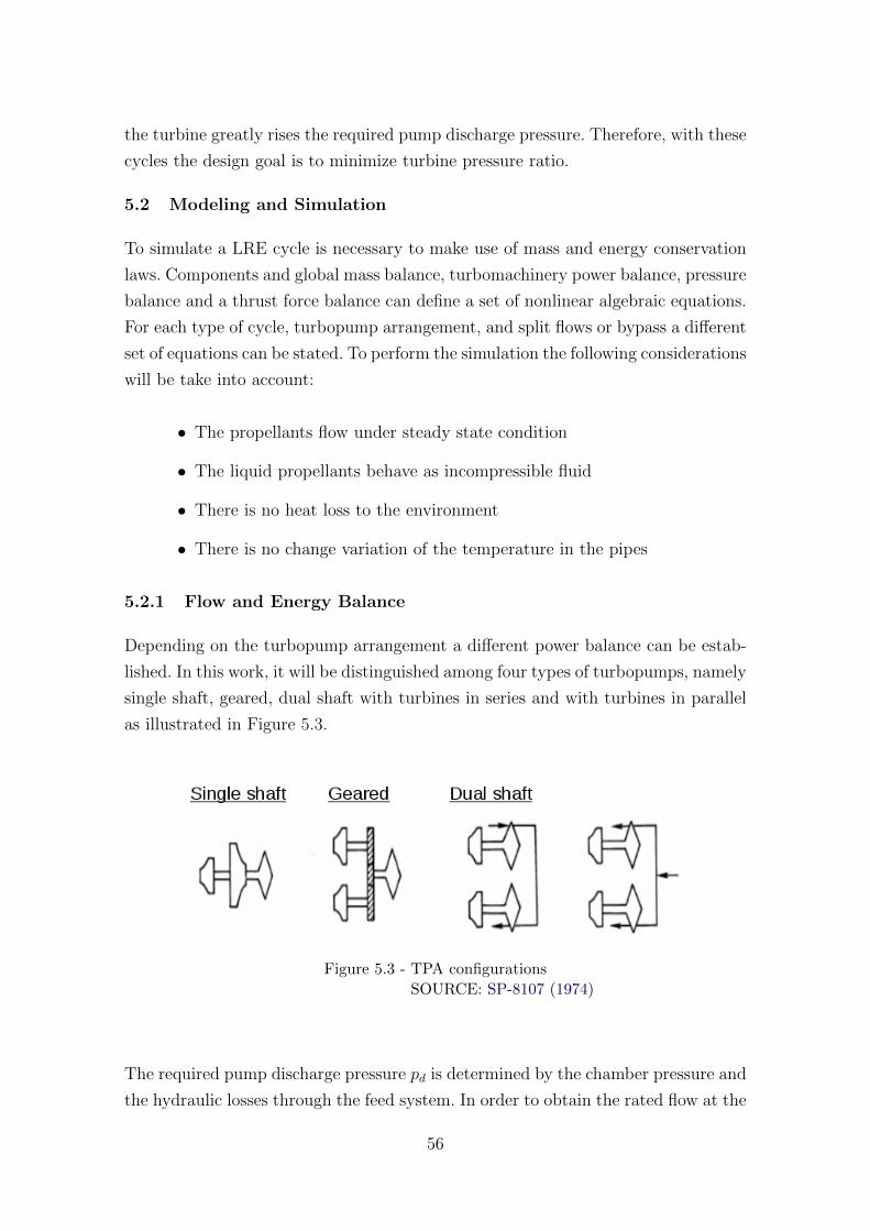
3.1 Turbopump configurations. . . . . . . . . . . . . . . . . . . . . . . . . . 18
3.2 Gas generator cycle with gases from turbine injected part way down the
skirt of the nozzle. . . . . . . . . . . . . . . . . . . . . . . . . . . . . . . 23
3.3 Pressure balance on the thrust chamber walls. . . . . . . . . . . . . . . . 26
3.4 Propellant combination performance. . . . . . . . . . . . . . . . . . . . . 30
3.5 Dump Cooling. . . . . . . . . . . . . . . . . . . . . . . . . . . . . . . . . 32
3.6 Theoretical vacuum specific impulse of dumped hydrogen through infinite
area ratio nozzle. . . . . . . . . . . . . . . . . . . . . . . . . . . . . . . . 33
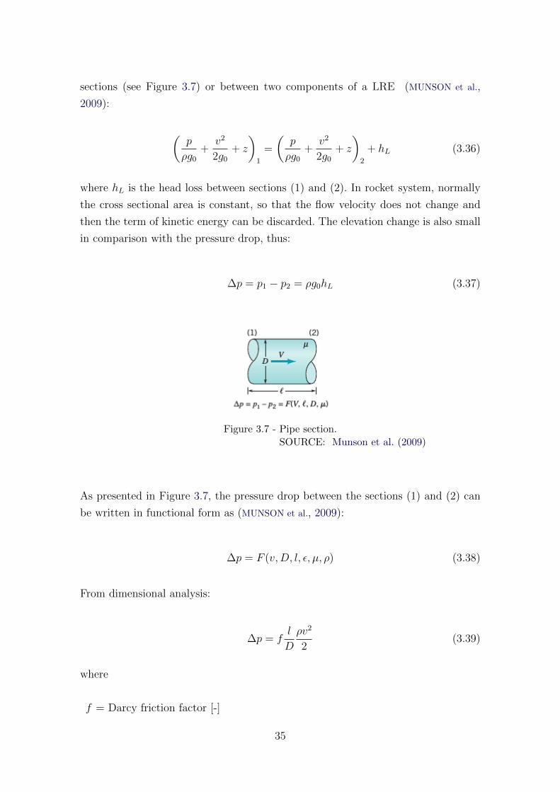
3.7 Pipe section. . . . . . . . . . . . . . . . . . . . . . . . . . . . . . . . . . 35
3.8 Pressure loss in a tap-off branch related to configuration of the branch. . 36
3.9 (a) Flow guide vanes in sharp elbows of pump inlet lines (b) Flow without
and with guide vanes. . . . . . . . . . . . . . . . . . . . . . . . . . . . . 36
4.1 Curve fit. . . . . . . . . . . . . . . . . . . . . . . . . . . . . . . . . . . . 44
4.2 Propellant tank configuration. . . . . . . . . . . . . . . . . . . . . . . . . 47
5.1 Open Cycles. (a) Gas Generator (b) Expander Bleed. . . . . . . . . . . . 54
5.2 Closed Cycles. (a) Expander Cycle (b) Staged Combustion. . . . . . . . . 55
5.3 TPA configurations . . . . . . . . . . . . . . . . . . . . . . . . . . . . . . 56
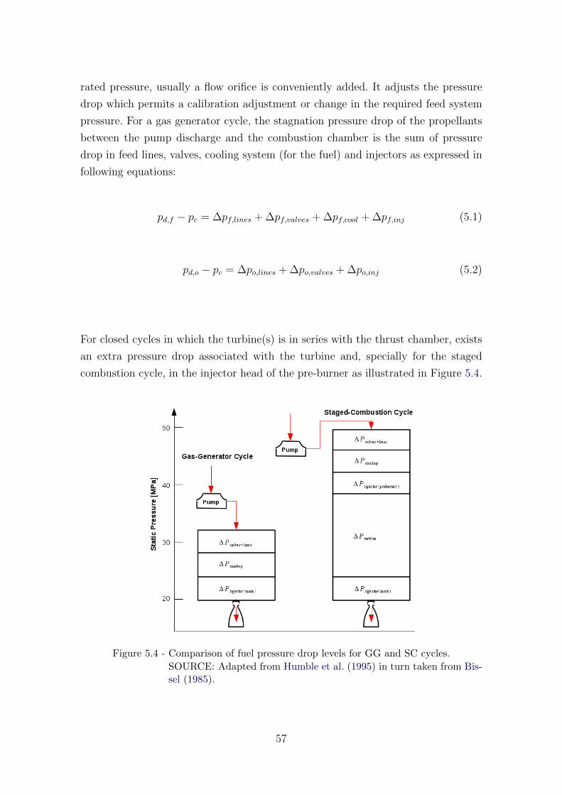
5.4 Comparison of fuel pressure drop levels for GG and SC cycles. . . . . . . 57
5.5 Propulsion model diagram. Possible input/output combinations. . . . . . 58
5.6 Flow scheme of a gas generator cycle. Seven unknown to be determined
are shown. . . . . . . . . . . . . . . . . . . . . . . . . . . . . . . . . . . . 61
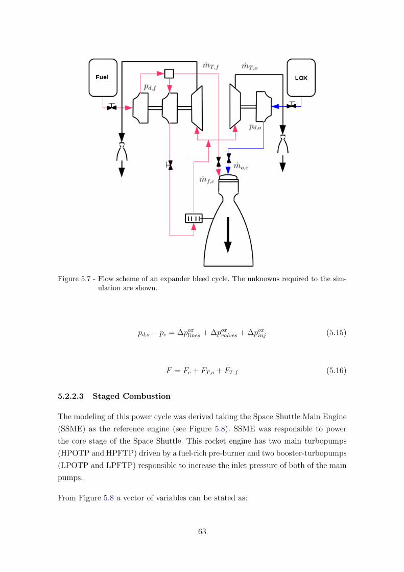
5.7 Flow scheme of an expander bleed cycle. The unknowns required to the
simulation are shown. . . . . . . . . . . . . . . . . . . . . . . . . . . . . . 63
xiii
Page 16
5.8 Flow scheme of staged combustion cycle. The unknowns required to the
simulation are shown. . . . . . . . . . . . . . . . . . . . . . . . . . . . . 65
5.9 Flow scheme of an expander cycle. The unknowns required to the simu-
lation are shown. . . . . . . . . . . . . . . . . . . . . . . . . . . . . . . . 67
6.1 Temperature in atmospheric layers. . . . . . . . . . . . . . . . . . . . . . 71
6.2 Drag coefficients. . . . . . . . . . . . . . . . . . . . . . . . . . . . . . . . 72
6.3 Reference Frames . . . . . . . . . . . . . . . . . . . . . . . . . . . . . . . 76
6.4 Planet-fixed and local horizon frames for atmospheric flight. . . . . . . . 78
6.5 External force resolved in the wind axes. . . . . . . . . . . . . . . . . . . 79
6.6 Schematic of Indirect Shooting Method. . . . . . . . . . . . . . . . . . . 84
6.7 Different Types of Direct Methods. . . . . . . . . . . . . . . . . . . . . . 85
7.1 UML Interface. . . . . . . . . . . . . . . . . . . . . . . . . . . . . . . . . 93
7.2 Dependency relationship between orbit class and aster class. . . . . . . . 93
7.3 UML - Single Shaft TPA. . . . . . . . . . . . . . . . . . . . . . . . . . . 95
7.4 UML - Dual Shaft TPA. . . . . . . . . . . . . . . . . . . . . . . . . . . . 96
7.5 UML - Thrust Chamber Assembly. . . . . . . . . . . . . . . . . . . . . . 96
7.6 UML diagram of a gas generator cycle. . . . . . . . . . . . . . . . . . . . 98
7.7 UML diagram of a staged-combustion liquid rocket engine. . . . . . . . . 99
7.8 UML - Launch Vehicle Model. . . . . . . . . . . . . . . . . . . . . . . . . 100
8.1 Simplified UML diagram representing the L75 rocket engine. . . . . . . . 102
8.2 L75 input/output. . . . . . . . . . . . . . . . . . . . . . . . . . . . . . . 103
8.3 Vulcain input/output. . . . . . . . . . . . . . . . . . . . . . . . . . . . . 104
8.4 HM7B input/output. . . . . . . . . . . . . . . . . . . . . . . . . . . . . . 106
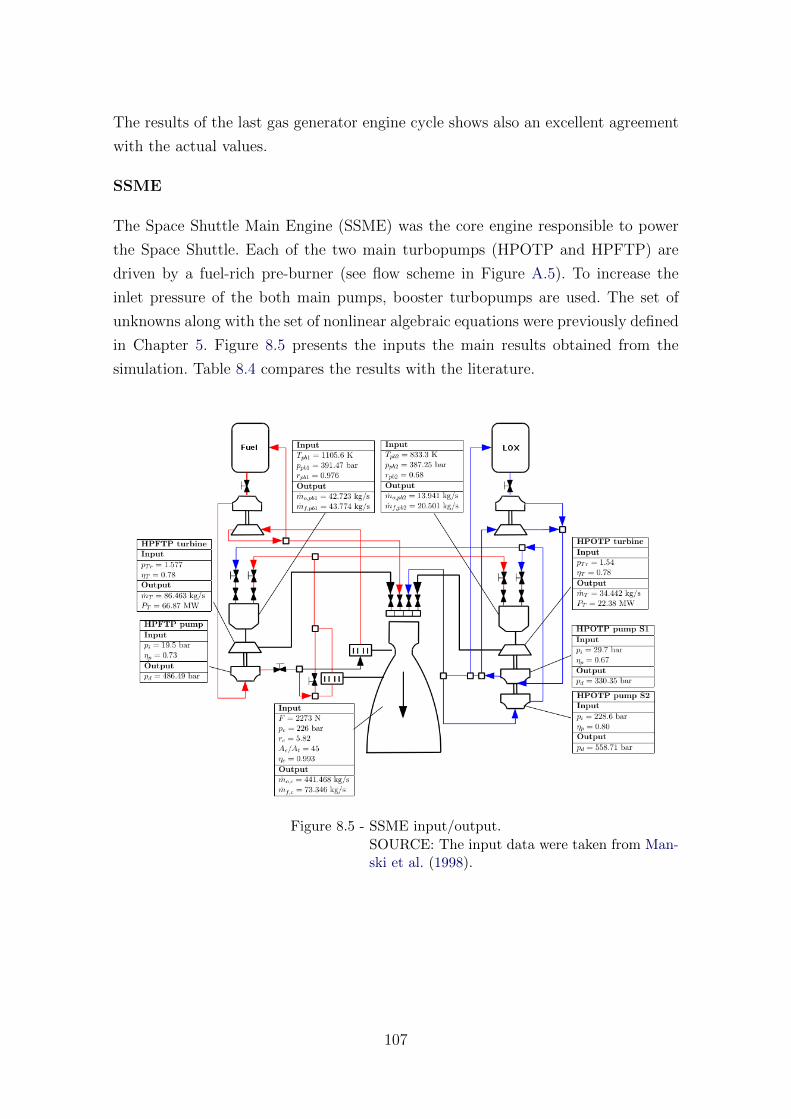
8.5 SSME input/output. . . . . . . . . . . . . . . . . . . . . . . . . . . . . . 107
8.6 Performance of the L75 rocket engine as function of the chamber pressure.109
9.1 VLS-1 design parameters. . . . . . . . . . . . . . . . . . . . . . . . . . . 112
9.2 Velocity profile of the VLS launch vehicle using first formulation of state
equations. . . . . . . . . . . . . . . . . . . . . . . . . . . . . . . . . . . . 113
9.3 Altitude profile of the VLS launch vehicle using first formulation of state
equations. . . . . . . . . . . . . . . . . . . . . . . . . . . . . . . . . . . . 114
9.4 Dynamic pressure profile of the VLS launch vehicle using first formulation
of state equations. . . . . . . . . . . . . . . . . . . . . . . . . . . . . . . 114
9.5 Velocity profile of the VLS launch vehicle using second formulation of
state equations. . . . . . . . . . . . . . . . . . . . . . . . . . . . . . . . . 116
9.6 Altitude profile of the VLS launch vehicle using second formulation of
state equations. . . . . . . . . . . . . . . . . . . . . . . . . . . . . . . . . 116
xiv
Page 17
9.7 Dynamic pressure profile of the VLS launch vehicle using second formu-
lation of state equations. . . . . . . . . . . . . . . . . . . . . . . . . . . . 117
9.8 Ground track. . . . . . . . . . . . . . . . . . . . . . . . . . . . . . . . . . 117
9.9 Data: European Launch vehicle. . . . . . . . . . . . . . . . . . . . . . . . 118
9.10 Altitude profile of the European Ariane 5. . . . . . . . . . . . . . . . . . 119
9.11 Velocity profile of the European Ariane 5. . . . . . . . . . . . . . . . . . 119
9.12 Comparison. . . . . . . . . . . . . . . . . . . . . . . . . . . . . . . . . . . 120
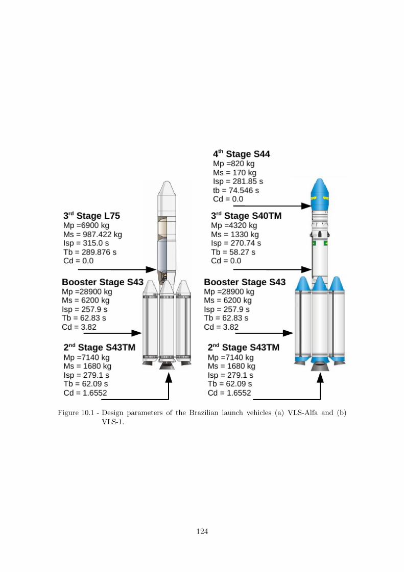
10.1 Design parameters of the Brazilian launch vehicles (a) VLS-Alfa and (b)
VLS-1. . . . . . . . . . . . . . . . . . . . . . . . . . . . . . . . . . . . . . 124
10.2 Relative velocity profile of the former and future Brazilian launch vehicle. 125
10.3 Altitude profile of the former and future Brazilian launch vehicle. . . . . 125
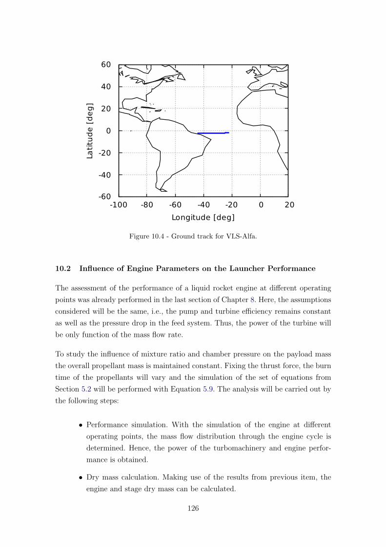
10.4 Ground track for VLS-Alfa. . . . . . . . . . . . . . . . . . . . . . . . . . 126
10.5 Key parameters of the L75 rocket engine. . . . . . . . . . . . . . . . . . . 127
10.6 Influence of the chamber pressure pc on (a) engine dry mass and (b) stage
dry mass. . . . . . . . . . . . . . . . . . . . . . . . . . . . . . . . . . . . 128
10.7 Influence of the chamber pressure pc on the payload mass. . . . . . . . . 128
10.8 Influence of the mixture ratio rc on (a) engine dry mass and (b) stage
dry mass. . . . . . . . . . . . . . . . . . . . . . . . . . . . . . . . . . . . 129
10.9 Influence of the mixture ratio rc on the payload mass. . . . . . . . . . . . 129
A.1 L75 scheme. . . . . . . . . . . . . . . . . . . . . . . . . . . . . . . . . . . 145
A.2 Flow schemes Vulcain. . . . . . . . . . . . . . . . . . . . . . . . . . . . . 146
A.3 Flow scheme HM7B. . . . . . . . . . . . . . . . . . . . . . . . . . . . . . 147
A.4 Flow scheme SSME. . . . . . . . . . . . . . . . . . . . . . . . . . . . . . 148
A.5 RL10-A-3A scheme. . . . . . . . . . . . . . . . . . . . . . . . . . . . . . . 149
xv
Page 19
LIST OF TABLES
Pag.
3.1 Typical design parameter values for turbopump of a liquid rocket engine. 22
4.1 Relations for the main engine’s mass of different types of rocket engine
cycles. . . . . . . . . . . . . . . . . . . . . . . . . . . . . . . . . . . . . . 41
4.2 Mass model validation. . . . . . . . . . . . . . . . . . . . . . . . . . . . . 44
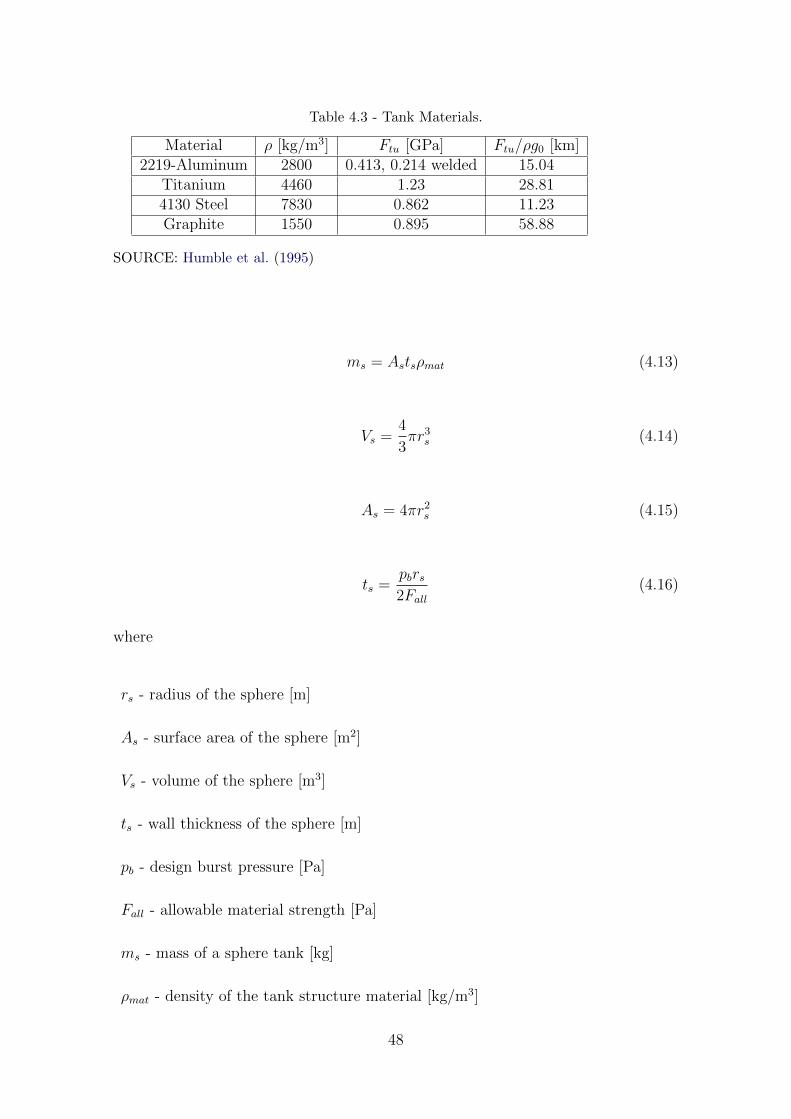
4.3 Tank Materials. . . . . . . . . . . . . . . . . . . . . . . . . . . . . . . . . 48
5.1 LRE with gas generator cycle. . . . . . . . . . . . . . . . . . . . . . . . . 60
5.2 LRE with expander bleed cycle. . . . . . . . . . . . . . . . . . . . . . . . 62
5.3 LRE with staged combustion cycle. . . . . . . . . . . . . . . . . . . . . . 64
5.4 LRE with expander cycle. . . . . . . . . . . . . . . . . . . . . . . . . . . 66
6.1 Standard Atmosphere (TEWARI, 2007). . . . . . . . . . . . . . . . . . . . 70
7.1 Comparison between object-oriented and function-oriented (procedural)
programming. . . . . . . . . . . . . . . . . . . . . . . . . . . . . . . . . . 92
7.2 Overview of the main components functionality of a liquid rocket engine
required in order to perform the simulation of the engine cycle. . . . . . 94
8.1 Verification of the simulated parameters of the L75: Comparison with the
literature. . . . . . . . . . . . . . . . . . . . . . . . . . . . . . . . . . . . 103
8.2 Verification of the simulated parameters of the Vulcain: Comparison with
the literature. . . . . . . . . . . . . . . . . . . . . . . . . . . . . . . . . . 105
8.3 Verification of the simulated parameters of the HM7B: Comparison with
the literature. . . . . . . . . . . . . . . . . . . . . . . . . . . . . . . . . . 106
8.4 Verification of the simulated parameters of the SSME: Comparison with
the literature. . . . . . . . . . . . . . . . . . . . . . . . . . . . . . . . . . 108
8.5 Values of specific impulse and nozzle expansion for different chamber
pressures. . . . . . . . . . . . . . . . . . . . . . . . . . . . . . . . . . . . 109
9.1 Values for state variables at start, inter-stage and end instants. . . . . . . 112
9.2 Optimized control parameters. . . . . . . . . . . . . . . . . . . . . . . . . 113
9.3 Values for state variables at start, inter-stage and end instants. . . . . . . 115
9.4 Optimized control parameters. . . . . . . . . . . . . . . . . . . . . . . . . 115
9.5 Optimized control parameters. . . . . . . . . . . . . . . . . . . . . . . . . 121
10.1 Data: Brazilian launch vehicle VLS . . . . . . . . . . . . . . . . . . . . . 123
xvii
Page 20
10.2 Data: Brazilian launch vehicle VLS-Alfa . . . . . . . . . . . . . . . . . . 123
xviii
Page 21
LIST OF ABBREVIATIONS
ASTOS – AeroSpace Trajectory Optimization SoftwareCEA – Chemical Equilibrium with ApplicationsDLR – German Aerospace CenterEC – Expander CycleEB – Expander Bleed CycleGA – Genetic AlgorithmGEO – Geostationary Earth OrbitGG – Gas Generator CycleHPOTP – High Pressure Oxidyzer TurbopumpHPFTP – High Pressure Fuel TurbopumpIAE – Institute of Aeronautics and SpaceLCC – Life-Cycle CostLEO – Low Earth OrbitLH2 – Liquid HydrogenLOX – Liquid OxygenLPOTP – Low Pressure Oxidyzer TurbopumpLPFTP – Low Pressure Fuel TurbopumpLRE – Liquid Rocket EngineNASA – National Aeronautics and Space AdministrationNLP – Non Linear Programming ProblemNPSH – Net Positive Suction headOOP – Object-Oriented ProgrammingPOST – Program to Optimize Simulated TrajectoryPSO – Particule Swarm OptimizationREDTOP – Rocket Engine Design Tool for Optimal PerformanceSC – Staged Combustion CycleSCORES – SpaceCraft Object-oriented Rocket Engine SimulationSQP – Sequential Quadratic ProgramSSME – Space Shuttle Main EngineTPA – Turbopump AssemblyTCA – Thrust Chamber AssmeblyUML – Unified Modeling LanguageVLS – Brazilian Launch Vehicle (Vehıculo Lancador de Satelites in Portuguese)
xix
Page 23
LIST OF SYMBOLS
A – azimuth [rad]a – thermal lapse rate [-]Ae – nozzle exit area [m2]At – throat area of the nozzle [m2]c – effective exhaust velocity [m/s]c∗ – characteristic velocity [m/s]CD – drag coefficient [-]CL – lift coefficient [-]Cf – thrust coefficient [-]D – pipe diameter [m]
– drag force [N]F – thrust force [N]f – Darcy friction factor [-]
– resultant force [N]G – gravitational constant [Nm2/kg2]g0 – standard gravitational acceleration [m/s2]hL – head loss [m]Hp – pump head rise [m]Isp – specific impulse [s]Ji(i = 1, 2, 3) – Jeffery’s constants [-]L – lift force [N]l – length of the pipe [m]m – mass [kg]M – molar mass [kg/mol]Mbody – Mass of a celestial body [kg]Nr – pump’s rotational speed [rad/s]Ns – stage-specific speed [(m/s)1/3/m0.75]m – mass flow rate [m/s]P – power [J/s]pa – ambient pressure [Pa]pd – discharge pressure [Pa]pe – nozzle exit pressure [Pa]pi – inlet pressure [Pa]Pi(i = 1, 2, 3) – Legendre polynomialspv – vapor pressure [Pa]pTr – turbine pressure ratio [-]Q – volume flow rate [m3/s]Re – equatorial radius of the Earth [km]Rp – polar radius of the Earth [km]Sref – reference area of the body [m2]
xxi
Page 24
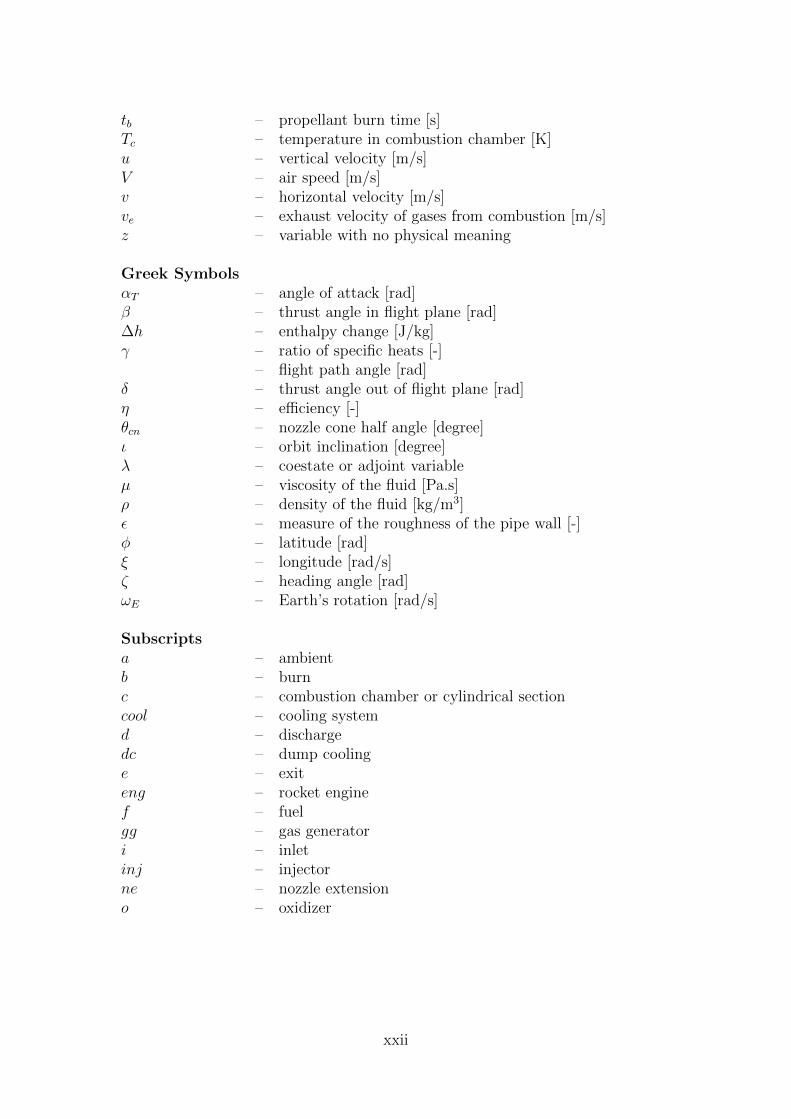
tb – propellant burn time [s]Tc – temperature in combustion chamber [K]u – vertical velocity [m/s]V – air speed [m/s]v – horizontal velocity [m/s]ve – exhaust velocity of gases from combustion [m/s]z – variable with no physical meaning
Greek SymbolsαT – angle of attack [rad]β – thrust angle in flight plane [rad]∆h – enthalpy change [J/kg]γ – ratio of specific heats [-]
– flight path angle [rad]δ – thrust angle out of flight plane [rad]η – efficiency [-]θcn – nozzle cone half angle [degree]ι – orbit inclination [degree]λ – coestate or adjoint variableµ – viscosity of the fluid [Pa.s]ρ – density of the fluid [kg/m3]ε – measure of the roughness of the pipe wall [-]φ – latitude [rad]ξ – longitude [rad/s]ζ – heading angle [rad]ωE – Earth’s rotation [rad/s]
Subscriptsa – ambientb – burnc – combustion chamber or cylindrical sectioncool – cooling systemd – dischargedc – dump coolinge – exiteng – rocket enginef – fuelgg – gas generatori – inletinj – injectorne – nozzle extensiono – oxidizer
xxii
Page 25
oa – overallpb – pre-burnerpl – payloadprop – propellantps – propellant systems – spherestruct – structuralt – throattp – turbopump
xxiii
Page 27
CONTENTS
Pag.
1 INTRODUCTION . . . . . . . . . . . . . . . . . . . . . . . . . . . 1
1.1 Motivation . . . . . . . . . . . . . . . . . . . . . . . . . . . . . . . . . . . 1
1.1.1 Design Phases . . . . . . . . . . . . . . . . . . . . . . . . . . . . . . . . 2
1.1.2 National Scenario . . . . . . . . . . . . . . . . . . . . . . . . . . . . . . 2
1.2 Objective . . . . . . . . . . . . . . . . . . . . . . . . . . . . . . . . . . . 3
1.3 Background - Basic Concepts in Space Technology . . . . . . . . . . . . . 4
1.3.1 Launch Vehicle . . . . . . . . . . . . . . . . . . . . . . . . . . . . . . . 4
1.3.2 Launch of a Satellite into Orbit . . . . . . . . . . . . . . . . . . . . . . 5
1.3.2.1 Ascent Trajectory . . . . . . . . . . . . . . . . . . . . . . . . . . . . 5
1.3.3 Rocket Propulsion . . . . . . . . . . . . . . . . . . . . . . . . . . . . . 6
1.4 Work Outline . . . . . . . . . . . . . . . . . . . . . . . . . . . . . . . . . 8
2 LITERATURE REVIEW . . . . . . . . . . . . . . . . . . . . . . . 11
2.1 Propulsion Performance . . . . . . . . . . . . . . . . . . . . . . . . . . . 11
2.2 Mass Modeling . . . . . . . . . . . . . . . . . . . . . . . . . . . . . . . . 14
2.2.1 Historical Background . . . . . . . . . . . . . . . . . . . . . . . . . . . 14
2.3 Trajectory Optimization . . . . . . . . . . . . . . . . . . . . . . . . . . . 15
2.3.1 Indirect Method . . . . . . . . . . . . . . . . . . . . . . . . . . . . . . 15
2.3.2 Direct Method . . . . . . . . . . . . . . . . . . . . . . . . . . . . . . . 15
2.3.3 Hybrid Method . . . . . . . . . . . . . . . . . . . . . . . . . . . . . . . 16
3 COMPONENTS MODELING . . . . . . . . . . . . . . . . . . . . 17
3.1 Turbopump . . . . . . . . . . . . . . . . . . . . . . . . . . . . . . . . . . 17
3.1.1 Pump . . . . . . . . . . . . . . . . . . . . . . . . . . . . . . . . . . . . 17
3.1.2 Turbine . . . . . . . . . . . . . . . . . . . . . . . . . . . . . . . . . . . 20
3.1.3 Booster Turbopump . . . . . . . . . . . . . . . . . . . . . . . . . . . . 24
3.2 Thrust Chamber . . . . . . . . . . . . . . . . . . . . . . . . . . . . . . . 24
3.2.1 Rocket-Thrust Equation . . . . . . . . . . . . . . . . . . . . . . . . . . 25
3.2.2 Specific Impulse and Effective Exhaust Velocity . . . . . . . . . . . . . 26
3.2.3 Thrust Coefficient and Characteristic Velocity . . . . . . . . . . . . . . 27
3.2.4 Real Rocket . . . . . . . . . . . . . . . . . . . . . . . . . . . . . . . . . 28
3.2.5 Approximate Equations for Parameters from Combustion . . . . . . . . 28
3.2.6 Performance Optimization . . . . . . . . . . . . . . . . . . . . . . . . . 29
xxv
Page 28
3.3 Gas Generator or Pre-burner . . . . . . . . . . . . . . . . . . . . . . . . 30
3.4 Injector Head . . . . . . . . . . . . . . . . . . . . . . . . . . . . . . . . . 31
3.5 Heat Exchanger . . . . . . . . . . . . . . . . . . . . . . . . . . . . . . . . 31
3.6 Pipe System: Feed Lines and Valves . . . . . . . . . . . . . . . . . . . . . 33
3.6.1 Feed Lines . . . . . . . . . . . . . . . . . . . . . . . . . . . . . . . . . . 34
3.6.2 Valves . . . . . . . . . . . . . . . . . . . . . . . . . . . . . . . . . . . . 36
4 MASS MODELING . . . . . . . . . . . . . . . . . . . . . . . . . . 39
4.1 Estimate Engine Mass . . . . . . . . . . . . . . . . . . . . . . . . . . . . 39
4.1.1 Simple Relations . . . . . . . . . . . . . . . . . . . . . . . . . . . . . . 39
4.1.2 Detailed Relations . . . . . . . . . . . . . . . . . . . . . . . . . . . . . 40
4.2 Propellant System Mass . . . . . . . . . . . . . . . . . . . . . . . . . . . 45
4.2.1 Simple Relations . . . . . . . . . . . . . . . . . . . . . . . . . . . . . . 45
4.2.2 Detailed Relations . . . . . . . . . . . . . . . . . . . . . . . . . . . . . 45
4.2.2.1 Propellant Tanks . . . . . . . . . . . . . . . . . . . . . . . . . . . . . 46
4.2.2.2 Propellant Mass . . . . . . . . . . . . . . . . . . . . . . . . . . . . . 50
4.3 Rocket Parameters . . . . . . . . . . . . . . . . . . . . . . . . . . . . . . 51
5 ROCKET ENGINE CYCLES MODELING . . . . . . . . . . . . 53
5.1 Basic Concepts . . . . . . . . . . . . . . . . . . . . . . . . . . . . . . . . 53
5.1.1 Open Cycles . . . . . . . . . . . . . . . . . . . . . . . . . . . . . . . . 54
5.1.2 Closed Cycles . . . . . . . . . . . . . . . . . . . . . . . . . . . . . . . . 55
5.2 Modeling and Simulation . . . . . . . . . . . . . . . . . . . . . . . . . . . 56
5.2.1 Flow and Energy Balance . . . . . . . . . . . . . . . . . . . . . . . . . 56
5.2.1.1 Flow Spliter . . . . . . . . . . . . . . . . . . . . . . . . . . . . . . . . 58
5.2.1.2 Input Parameters Selection . . . . . . . . . . . . . . . . . . . . . . . 58
5.2.2 Cycle Balance . . . . . . . . . . . . . . . . . . . . . . . . . . . . . . . . 58
5.2.2.1 Gas Generator Cycle . . . . . . . . . . . . . . . . . . . . . . . . . . . 59
5.2.2.2 Expander Bleed Cycle . . . . . . . . . . . . . . . . . . . . . . . . . . 62
5.2.2.3 Staged Combustion . . . . . . . . . . . . . . . . . . . . . . . . . . . 63
5.2.2.4 Expander Cycle . . . . . . . . . . . . . . . . . . . . . . . . . . . . . 66
6 TRAJECTORY MODELING AND OPTIMIZATION . . . . . . 69
6.1 Atmosphere Model . . . . . . . . . . . . . . . . . . . . . . . . . . . . . . 69
6.1.1 Standard Atmosphere . . . . . . . . . . . . . . . . . . . . . . . . . . . 69
6.2 Aerodynamics . . . . . . . . . . . . . . . . . . . . . . . . . . . . . . . . . 70
6.2.1 Aerodynamics Coefficients . . . . . . . . . . . . . . . . . . . . . . . . . 71
6.3 Gravitational Model . . . . . . . . . . . . . . . . . . . . . . . . . . . . . 73
xxvi
Page 29
6.4 Equations of the Translational Motion . . . . . . . . . . . . . . . . . . . 74
6.4.1 First Formulation . . . . . . . . . . . . . . . . . . . . . . . . . . . . . . 75
6.4.2 Second Formulation . . . . . . . . . . . . . . . . . . . . . . . . . . . . 77
6.5 Guidance Programme . . . . . . . . . . . . . . . . . . . . . . . . . . . . . 80
6.6 Path Constraints . . . . . . . . . . . . . . . . . . . . . . . . . . . . . . . 81
6.7 Optimization . . . . . . . . . . . . . . . . . . . . . . . . . . . . . . . . . 82
6.7.1 Background . . . . . . . . . . . . . . . . . . . . . . . . . . . . . . . . . 82
6.7.1.1 Optimal Control Problem . . . . . . . . . . . . . . . . . . . . . . . . 82
6.7.2 Methodology . . . . . . . . . . . . . . . . . . . . . . . . . . . . . . . . 85
6.7.2.1 First Approach - Direct Method . . . . . . . . . . . . . . . . . . . . 85
6.7.2.2 Second Approach - Hybrid Method . . . . . . . . . . . . . . . . . . . 87
7 PROGRAMME SETUP . . . . . . . . . . . . . . . . . . . . . . . . 91
7.1 Object-oriented Programming (OOP) . . . . . . . . . . . . . . . . . . . . 91
7.2 Unified Modeling Language (UML) . . . . . . . . . . . . . . . . . . . . . 92
7.3 Overview of the Main Components Functionality . . . . . . . . . . . . . 93
7.4 Engine Components Assembly Modeling . . . . . . . . . . . . . . . . . . 95
7.4.1 Turbopump Assembly Modeling . . . . . . . . . . . . . . . . . . . . . . 95
7.4.2 Thrust Chamber Assembly Modeling . . . . . . . . . . . . . . . . . . . 96
7.5 Engine Cycle Modeling . . . . . . . . . . . . . . . . . . . . . . . . . . . . 97
7.6 Launch Vehicle Modeling . . . . . . . . . . . . . . . . . . . . . . . . . . . 99
8 RESULTS 1: SIMULATION OF LIQUID ROCKET ENGINES 101
8.1 Performance of a Liquid Rocket Engine . . . . . . . . . . . . . . . . . . . 101
8.2 Sensitivity Analysis . . . . . . . . . . . . . . . . . . . . . . . . . . . . . . 108
9 RESULTS 2: TRAJECTORY SIMULATION . . . . . . . . . . . 111
9.1 Direct Method . . . . . . . . . . . . . . . . . . . . . . . . . . . . . . . . 111
9.1.1 VLS launch Vehicle . . . . . . . . . . . . . . . . . . . . . . . . . . . . . 111
9.1.2 Ariane 5 Launch Vehicle . . . . . . . . . . . . . . . . . . . . . . . . . . 118
9.2 Hybrid Method . . . . . . . . . . . . . . . . . . . . . . . . . . . . . . . . 120
10 MISSION ANALYSIS . . . . . . . . . . . . . . . . . . . . . . . . . 123
10.1 Flight Simulation . . . . . . . . . . . . . . . . . . . . . . . . . . . . . . . 123
10.2 Influence of Engine Parameters on the Launcher Performance . . . . . . 126
11 CONCLUSION AND SUGGESTIONS . . . . . . . . . . . . . . . 131
11.1 Conclusion . . . . . . . . . . . . . . . . . . . . . . . . . . . . . . . . . . . 131
11.1.1 Contribution of This Work . . . . . . . . . . . . . . . . . . . . . . . . . 132
xxvii
Page 30
11.2 Suggestions . . . . . . . . . . . . . . . . . . . . . . . . . . . . . . . . . . 133
REFERENCES . . . . . . . . . . . . . . . . . . . . . . . . . . . . . . . 135
ANEXO A - Flow Schemes of Liquid Rocket Engines . . . . . . . . . 145
A.1 L75 . . . . . . . . . . . . . . . . . . . . . . . . . . . . . . . . . . . . . . . 145
A.2 Vulcain . . . . . . . . . . . . . . . . . . . . . . . . . . . . . . . . . . . . 145
A.3 HM7B . . . . . . . . . . . . . . . . . . . . . . . . . . . . . . . . . . . . . 146
A.4 SSME . . . . . . . . . . . . . . . . . . . . . . . . . . . . . . . . . . . . . 147
A.5 RL10-A-3A . . . . . . . . . . . . . . . . . . . . . . . . . . . . . . . . . . 148
xxviii
Page 31
1 INTRODUCTION
1.1 Motivation
Although it has been almost six decades since the Soviet Union put the first artificial
satellite into orbit, launch vehicles are still based on the fundamental technologies
developed at the dawn of the space era.
Space launch systems are composed of a large number of components grouped into a
hierarchy of subsystems. The performance of the vehicle depends on the individual
performance of each of the subsystems which in turn depend on material properties
and design parameters. Changes in design parameters are propagated throughout
the cluster hierarchy of subsystems and components, flight trajectory and payload
capability (HINCKEL, 1995).
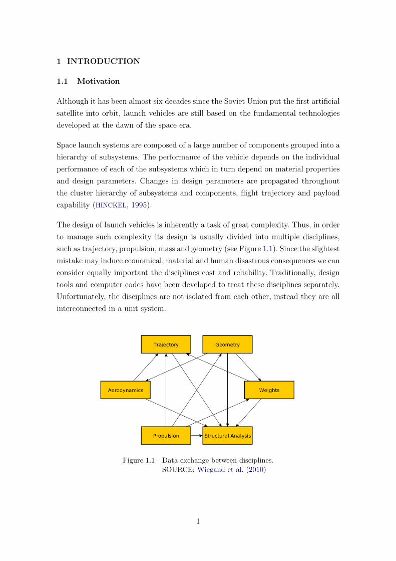
The design of launch vehicles is inherently a task of great complexity. Thus, in order
to manage such complexity its design is usually divided into multiple disciplines,
such as trajectory, propulsion, mass and geometry (see Figure 1.1). Since the slightest
mistake may induce economical, material and human disastrous consequences we can
consider equally important the disciplines cost and reliability. Traditionally, design
tools and computer codes have been developed to treat these disciplines separately.
Unfortunately, the disciplines are not isolated from each other, instead they are all
interconnected in a unit system.
Figure 1.1 - Data exchange between disciplines.
SOURCE: Wiegand et al. (2010)
1
Page 32
1.1.1 Design Phases
The design phases for most systems including launch vehicles can be divided into
three project phases: conceptual, preliminary and detailed. Specifically, it has been
shown that 80 % a vehicle’s life-cycle cost (LCC) is determined by the conceptual
design while efforts for optimization in further steps only result in less significant
improvement (HAMMOND, 2001). This could be translated in the statement: “engi-
neering can never right a poor concept selection” (Hammond (2001) in turn taken
from Pugh (1991)).
1.1.2 National Scenario
In an attempt to get autonomous access to space, starting from 1964 Brazil has
developed a series of sounding (research) rockets, named Sonda I, II, III, and IV
in which were the basis for building the Brazilian Satellite Launch Vehicle VLS-1
(Veıculo Lancador de Satelite - in Portuguese). To date, three prototypes have been
built and two launches attempted. Unfortunately due to failures, the vehicle however
could not be qualified up to now. The tragedy occurred in the launch pad in 2003
affected drastically the launcher program and more than one decade later there was
no attempt to a new launching. Brazil has a strategically located launch site in the
proximity of the equator called Alcantara Launch Center. Due to its prime location,
fuel consumption for launching satellites into equatorial orbit (e.g., communication
satellites in GEO orbit) is lower when compared to launch sites located at higher
latitudes.
The Brazilian space program has been aimed at vehicles using solid propellants with
launch capability limited to a few hundred kilograms into Low Earth Orbit (LEO).
To enlarge the launch envelope and payload mass to get higher orbits and also to
improve the launch injection accuracy, rocket engines driven by liquid propulsion
are not an option, but a must. The propellant choice, cycles, design parameters and
structural materials involves countless simulations and trade-off studies. During the
simulations and trade-off studies phase, the availability of a versatile tool for this
purpose is very useful. The development of the tool itself can also be used as a
learning tool and improvement of researchers, students and engineers who will be
further engaged in the program.
A program for the development of a liquid rocket engine is currently being carried
out at Aeronautics and Space Institute (IAE) to be used in the upper stage of the
Brazilian launch vehicle. The idea is to replace the last two solid stages of the VLS-
2
Page 33
1 launch vehicle by a single liquid rocket stage (see Figure 1.2). The LRE named
L75 will be capable of reaching a thrust range of (75± 5) kN using the propellants
combination LOX/Ethanol.
Figure 1.2 - Brazilian launch vehicle VLS-Alfa with highlighted L75 rocket engine.
SOURCE: The circulated rocket engine was taken from Almeida and Pagli-uco (2014) and the launch vehicle from Moraes Junior et al. (2011)
1.2 Objective
The purpose of this work is to develop a tool which can be easily reused and extended
to model and simulate a launch vehicle. In the framework of this thesis the focus will
be on propulsion system and trajectory. Thus, the tool is intended to be capable of
modeling and simulating different configurations of liquid rocket engines, modeling
and optimizing flight trajectory until orbit injection, and analyzing the influence of
engines parameters on the trajectory. Despite the large number of operational launch
vehicles, they usually consist of basic components and subsystems. In other words
a launch vehicle is an assembly of stages which in turn is divided into propellant
system and engine (for a liquid rocket engine), and the engine is an assembly of
basic components such as pumps, turbines, and combustion chamber. Then in order
3
Page 34
to permit a better extensibility and reusability of the codes, a modular approach
is chosen. Mathematical models for determination of the mass and performance of
liquid rocket engine cycle as well as the complete launch vehicle will be described and
discussed. With the engine design parameters and the mass models of the vehicle
along with models for atmosphere and gravitational field, the flight trajectory can
be determined. The launch vehicle performance will be measured by payload mass
for a given mission.
1.3 Background - Basic Concepts in Space Technology
1.3.1 Launch Vehicle
A launch vehicle is a space rocket used to carry a payload from the Earth’s surface
to outer space. The launch vehicles can be classified as reusable, when it is used
in more than one mission, and expendable when they are used for a single mission
(the stages are being discarded in certain phases of the ascent trajectory). The most
famous reusable launch vehicle is the American Space Shuttle. Although, in fact it is
partially reusable since the external tank storing liquid hydrogen and liquid oxygen
is expendable. In Figure 1.3 some launch vehicles of the world are shown.
Figure 1.3 - Launch Vehicles in the world.
SOURCE: Encyclopaedia Britannica (2015)
4
Page 35
In order to make use of atmospheric oxygen during the ascent flight to replace the
heavy oxidizer propellant (LOX) of a liquid rocket engine (LRE), and accordingly,
reducing the gross lift-off mass (GLOW), air-breathing launch vehicles have been re-
cently studied (MUSIELAK, 2012; SEGAL, 2004). However, the technology to develop
such a propulsion system which condenses the air in a split second and extracts LOX
still represents a task of great challenge in current engineering, thus so far, all the
operational launch vehicles store their propellant combination inside tanks before
the flight.
1.3.2 Launch of a Satellite into Orbit
The injection of a satellite into orbit is normally done by a multistage rocket. There
are basically two types of launching, by direct ascent and through a parking orbit.
The parking orbit is a temporary LEO (Low Earth Orbit), which has an altitude
of approximately 200 km, staying just above the denser layers of the atmosphere
(CORNELISSE et al., 1979). There are several reasons to make use of a parking orbit,
among them we can mention the increased launch window and missions to geosta-
tionary orbit. The inclination of the desired orbit ι depends on the latitude of the
launch site φ, and azimuth A (TEWARI, 2007):
cos ι = cosφ sinA (1.1)
Eq. 1.1 can be deduced from spherical trigonometry to the triangle formed by arcs
MO, ON and NM , as shown in Figure 1.4.
From Eq. 1.1 is evident that the smallest possible inclination of the orbit is achieved
when the rocket is launched eastward, i.e., when A = 90. Thus, the orbit inclination
will never be less than the launch latitude.
1.3.2.1 Ascent Trajectory
During the ascent trajectory, the vehicle performs five distinct phases in its way
from the launch pad to orbit (Figure 1.5):
• Vertical ascent: It needs to gain altitude quickly to minimize the gravita-
tional losses. Roll maneuver aligns launch azimuth with the correct orbital
plane.
• Pitch over: Begin to gain velocity downrange (horizontally).
5
Page 36
Figure 1.4 - Planet-fixed and local horizon frames.
SOURCE: Tewari (2007)
• Gravity turn: Gravity pulls the launch vehicle’s trajectory toward hori-
zontal.
• Ballistic (Optional): Non-powered. No control or just attitude.
• Orbital: Out of atmosphere. Accelerate the vehicle to gain the necessary
horizontal velocity to achieve orbit energy.
1.3.3 Rocket Propulsion
There are many reports and fundamental books that address propulsive systems of
launch vehicles, among them we can cite Huzel and Huang (1992), Hill and Peterson
(1992), Humble et al. (1995) and Sutton and Biblarz (2010). In general, a stage of
a launch vehicle consists of the following systems: structure, propulsion system,
propellant system and on-board equipment. A propulsion system which extracts
energy from combustion of liquid propellants is designed as liquid rocket engine
(LRE) and consists of the following subsystems:
• Thrust chamber
• Feed system
• Control system and valves
6
Page 37
Figure 1.5 - Flight phases of the European Ariane 5 launch vehicle.
SOURCE: Arianespace (2011)
The thrust chamber assembly consists of injector head, combustion chamber, nozzle,
igniter and cooling system. In the thrust chamber the propellants which come from
the feed system are injected, mixed, burned, and converted into hot gases at high
speeds. By the principle of conservation of energy, we can understand that in the
thrust chamber takes place a conversion of random motion of molecules at high
speeds (heat) in an ordered flow of gases at high speed (kinetic energy).
The feed system of a liquid rocket engine can be classified in two categories, i.e.,
pressure-fed and turbopumps-fed (Figure 1.6). In pressure-fed are used pressure
accumulators so that one can proceed the pressurization of the propellant tanks.
Because the entire tank is subjected to pressurization throughout the operation, their
application is restricted to engines which employ relatively low chamber pressure,
and lower thrust accordingly. This is due to the strong increase in the weight of the
tanks caused by required structural loads. (Figure 1.6a). For a turbopump system,
the pump, either axial or radial, is always coupled to one turbine, which in turn
is driven by working fluid from a gas generator. This allows to make use of lighter
tanks, since they are not under high internal pressures. Consequently, this engine can
7
Page 38
operate at higher chamber pressures, which results in increased thrust (Figure 1.6b).
Figure 1.6 - Feed system: (a) Pressure-fed (b) Turbopump-fed.
SOURCE: Sutton and Biblarz (2010)
1.4 Work Outline
To give an overview of what comes next in this work, the following chapters can be
divided in:
• Literature Review (Chapter 2). The focus of this chapter is to present
the main tools used in the literature and by the industry to model space
systems.
• Mathematical Modeling (Chapters 3-6). These Chapters are intended to
expose all the equations and technical recommendations which are neces-
sary to model a launch system.
• Programme Architecture (Chapter 7). This topic is responsible for gather-
ing all information contained in Chapters 3-6 and to explicit the commu-
8
Page 39
nication between systems, subsystems and components.
• Results (Chapters 8-10). These chapters are designed to show the applica-
bility and limitations of the developed codes.
• Conclusion (Chapter 11). The conclusions about the main results and sug-
gestions for future works are given in the last chapter of this work.
9
Page 41
2 LITERATURE REVIEW
In the second chapter of this Thesis will be discussed the historical background of
design for the disciplines trajectory, mass and performance for launch vehicles along
with the main tools developed during the last decades.
2.1 Propulsion Performance
This section begins with a short description of the well-known tool to calculate
engine performance CEA and then it follows with historical background of the most
notable works and tools developed from them, namely:
• SEQ
• EcoSimPRO
• REDTOP
• SCORES/SCORES-II
CEA
CEA, which stands for Chemical Equilibrium with Applications is a recognized
standard program for chemical equilibrium calculation. The tool calculates com-
plex chemical equilibrium product concentrations from any set of reactants and
determines thermodynamics and transport properties for the product mixture. The
program open source is freely distributed on the website NASA Glenn Research
Center (2010), where you can find a well documented report describing the the-
oretical principles (GORDON; MCBRIDE, 1994) and the user’s manual (GORDON;
MCBRIDE, 1996). Applications include:
• theoretical rocket performance (which is, of course, the one of interest in
this work),
• assigned thermodynamic states,
• Chapman-Jouguet detonations, and
• shock-tube parameters for incident and reflected shocks.
11
Page 42
SEQ and LRP2
One of the most important and robust tools for vehicle/propulsion analysis was de-
veloped when DLR and NASA combined computer codes to provide a capability to
optimize rocket engines cycles and its parameters as well as launch vehicles consid-
ering the coupling between them. In many publications you can find applications of
this tool (amongst them we can cite Manski and Martin (1990), Manski and Martin
(1991), Goertz (1995), Manski et al. (1998), Burkhardt et al. (2002), Sippel et al.
(2003), Burkhardt et al. (2004), Sippel et al. (2012)).
SCORES and SCORES-II
SCORES, which stands for SpaceCraft Object-oriented Rocket Engine Simulation,
is a web-based tool suitable to use for use in conceptual level spacecraft and launch
vehicle design. The tool is written in C++. Performance parameters provided by
SCORES are thrust, specific impulse and thrust to weight ratio. Initially, the tool
was created to support only LOX/LH2 propellants combination, but this was later
expanded to include a number of hydrocarbon fuels. SCORES does not model the
powerhead, instead works similar to CEA regarding its equilibrium analysis and
capabilities (WAY; OLDS, 1998; WAY; OLDS, 1999). Later this design tool would be-
come commercial with its capabilities greatly expanded and now with the name
SCORES-II (BRADFORD, 2002).
REDTOP
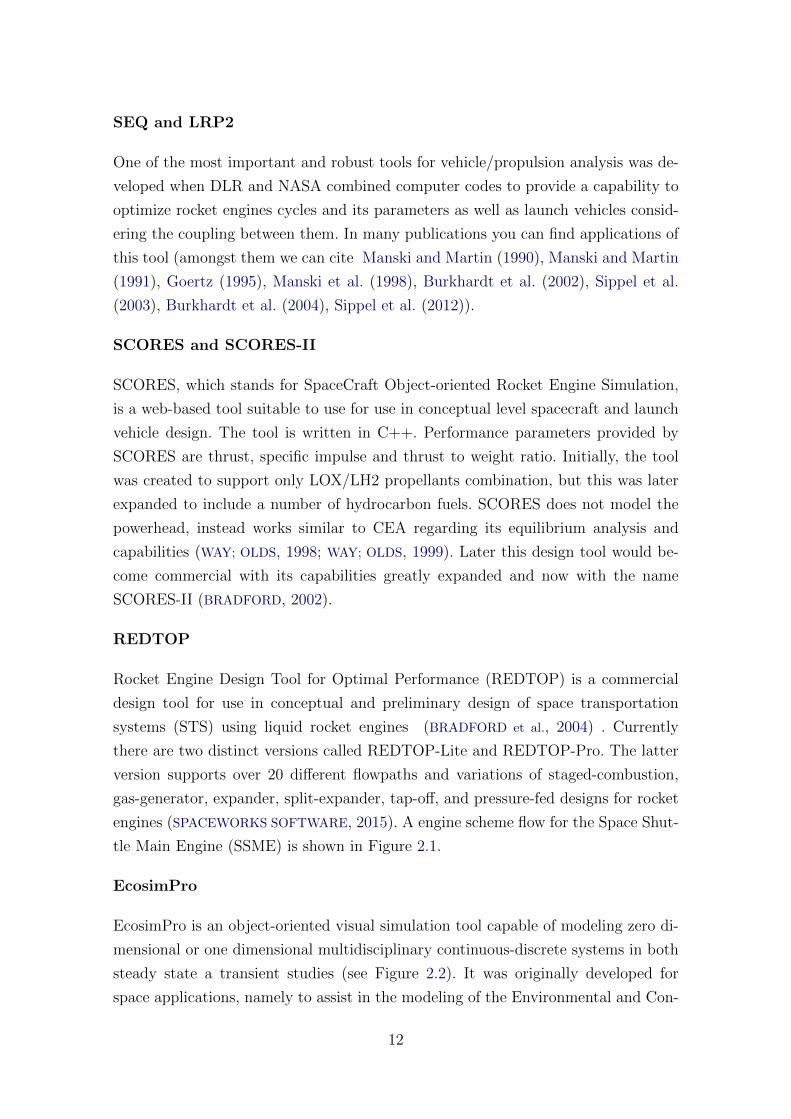
Rocket Engine Design Tool for Optimal Performance (REDTOP) is a commercial
design tool for use in conceptual and preliminary design of space transportation
systems (STS) using liquid rocket engines (BRADFORD et al., 2004) . Currently
there are two distinct versions called REDTOP-Lite and REDTOP-Pro. The latter
version supports over 20 different flowpaths and variations of staged-combustion,
gas-generator, expander, split-expander, tap-off, and pressure-fed designs for rocket
engines (SPACEWORKS SOFTWARE, 2015). A engine scheme flow for the Space Shut-
tle Main Engine (SSME) is shown in Figure 2.1.
EcosimPro
EcosimPro is an object-oriented visual simulation tool capable of modeling zero di-
mensional or one dimensional multidisciplinary continuous-discrete systems in both
steady state a transient studies (see Figure 2.2). It was originally developed for
space applications, namely to assist in the modeling of the Environmental and Con-
12
Page 43
Figure 2.1 - Redtop: SSME.
SOURCE: Spaceworks Software (2015)
trol Life Support Systems (ECLSS) for European Space Agency (ESA)’s HERMES
and COLUMBUS projects, however today one can find applications in a wide range
of fields. The first version of the tool was released in 1993. The tool employs a
set of multidisciplinary libraries in which allow components to be created that mix
disciplines such as mechanical, electrical, fluids, control, etc (ECOSIMPRO, 2015).
LiRa
Recently, in his Master Thesis, Ernst (2014) developed a tool to simulate liquid
rocket engines at steady conditions called LiRa (Liquid Rocket Engine Analysis).
The cycle balance differs from the traditional approach in the sense of instead of
creating a system of nonlinear equations based on power, flow and pressure balance,
his modeling starts from the thrust chamber.
13
Page 44
Figure 2.2 - EcosimPro Screeshot.
SOURCE: Ecosimpro (2015)
2.2 Mass Modeling
Most of the modeling approaches rely on historical data for comparison to the ana-
lytic equations, so that correction factors can be estimated. Because of this statistical
dependency, usually these models are relatively inaccurate.
2.2.1 Historical Background
To identify the coupling of nominal rocket design parameters on the trajectory
Verderaime (1964) developed a parametric method to derive approximate equations
for large liquid rocket engine mass and envelope. The engine mass was calculated by
the sum of three subsystems; turbopump, rocket chamber and accessories. To allow
mixture ratio shifts and propellant mass throttling performance equations which are
well known in the literature were modified.
Felber (1979) presents an empirical/analytical method to determine the mass of
the main components of a liquid rocket engines along with historical data to esti-
14
Page 45
mate the engine mass. Firstly detailed expressions for the components were derived:
turbopump, injector, combustion chamber, nozzle and valves; and then taking the
propellants combination LOX/LH2 simplified relations were achieved. Finally the
engine mass is calculated summing all the main components multiplied by a correc-
tion factor to take into account the remaining elements. To determine the correction
factor it was considered the engines HM7, H20, RL-10, SSME, J-2 and ASE.
Using a data base with 51 LRE, linear, quadratic, power law and logarithmic curves
were analyzed in Castellini (2012). The best resulting regression in terms of quadratic
fit error for each technology were implemented within the propulsion models.
Using historical data from 43 rocket engines and taking into account the type of pro-
pellant, chamber pressure, the nozzle area expansion ratio, and the number o thrust
chamber, Zandbergen (2015) presented simple relations to compute engine mass
making distinction with one use pressure-fed, turbopump fed, and if the propellants
are storable, cryogenic or semi-cryogenic.
2.3 Trajectory Optimization
In order to get the best performance of a given launch vehicle, and consequently, to
make the access to space less costly, trajectory optimization techniques has been for
decades a subject of intense research. Trajectory optimization can be categorized
basically into direct and indirect methods. In Betts (1999) and Rao (2009a) was
made a comprehensive discussion about both of two methods.
2.3.1 Indirect Method
The reason for this method to be called“indirect”comes from the strategy to convert
the original optimal control problem into a boundary-value problem. The most com-
mon indirect methods found in the literature are the shooting method, the multiple-
shooting method, and collocation methods as one can see in former reports (BROWN
et al., 1969; TEREN; SPURLOCK, 1966), recent works as in the paper of Miele (2003)
and in the Master thesis of Zerlotti (1990) which uses the algorithm BNDSCO
(OBERLE; GRIMM, 1990).
2.3.2 Direct Method
Presumably because of the possibility of solving complex problems with a minimum
effort of mathematical analysis, this method is the one chosen for most of the re-
searchers (BUENO NETO, 1986; HARGRAVES; PARIS, 1987; HERMAN; CONWAY, 1996;
15
Page 46
SEYWALD, 1994; SILVA, 1995; BALESDENT, 2011). One of the most popular soft-
ware used extensively in many publications is called POST (Program to Optimize
Simulated Trajectories) (BRAUER et al., 1977).
In the framework of this method, the problem is characterized by a set of parameters
which define the control law. This problem is a typical Non Linear Programming
Problem (NLP) and can be solved using classical Gradient-based methods (deter-
ministic methods) such as Sequential Quadratic Program (SQP) or by heuristic
methods. According to Betts (1999), heuristic optimization algorithms are not com-
putationally competitive with gradient methods. Even though presumably due to
ease of implementation without a detailed understanding of the system, in the last
two decades a lot of papers using Particle Swarm Optimization (PSO), genetic algo-
rithms (GA) among others were applied to solve trajectory optimization problems.
As for indirect methods, the direct methods can be categorized in direct (multiple)
shooting or collocation. In the case where only the control variables are adjusted
by a function, the method is called a shooting method. When both the state and
control are parameterized, the method is called a collocation method. A well-known
software developed by the University of Stuttgart which addresses the direct col-
location method is the AeroSpace Trajectory Optimization Software (ASTOS). For
either direct or indirect approaches, perhaps the most important benefit gained from
a multiple shooting formulation compared to its precursor (single shooting) is en-
hanced robustness.
2.3.3 Hybrid Method
To take advantage of both methods previously described, a hybrid method can
also be considered (STRYK; BULIRSCH, 1992; PONTANI; TEOFILATTO, 2014; GATH;
CALISE, 2001; GATH, 2002). The idea behind this approach is to divide the flight
trajectory into two distinct phases, namely atmospheric and exo-atmospheric phase,
applying the direct method in the first phase and indirect method in the second one.
Here, exo-atmospheric phase means that the vehicle is virtually in vacuum space,
i.e., the aerodynamic effects can be ignored.
Pontani and Teofilatto (2014) proposed a simple method to evaluate the perfor-
mance of multistage launch vehicles for given structural data, aerodynamic and
propulsive parameters.
16
Page 47
3 COMPONENTS MODELING
The common components for all liquid rocket engine turbopump-fed are pumps,
turbine(s), valves, pipes and thrust chamber. Depending on the configuration a gas
generator (for gas generator cycle), a pre-burner(s) (for staged combustion cycle) and
booster-pumps can be found as well. This chapter presents the modeling of the main
components of a liquid rocket engine which will be essential to model and simulate
the LRE cycles. Thus the design equations, the design parameters, limitations and
restrictions of each component will be presented and discussed.
3.1 Turbopump
The turbopump assembly (TPA) is required when it is desired a higher pressure in
the combustion chamber, i.e, when it is dealing with launch vehicles. Usually if the
density of the propellants are relatively close, an arrangement with single shaft TPA
can be applied. However, when it is dealing with propellants with strongly different
densities as the case of the combination LOX/LH2, a dual shaft TPA is required.
A TPA with two turbines (dual shaft) is still distinguished between configurations
working in series and working in parallel. There is still a configuration using gear
case, but this configuration implies in a more complicated design and then a single
shaft TPA is commonly preferred. Schematics of typical turbopump arrangements
are presented in Figure 3.1.
3.1.1 Pump
For space application weight is a key parameter, so centrifugal pumps are preferred
because they can handle a large amount of mass flow rate. Nevertheless axial and
mixed pumps are used. The required pump mass flow is parameterized by the engine
design parameters; thrust, effective exhaust velocity and mixture ratio, and propel-
lant densities. Assuming steady flow, the pump basically increases the Bernoulli
head between the pump inlet and outlet (WHITE, 1998):
Hp =
(p
ρg0
+v2
2g0
+ z
)discharge
−(
p
ρg0
+v2
2g0
+ z
)inlet
(3.1)
For a liquid rocket engine the terms in the right side related to kinetic [v2/2g0] and
potential energy [z] can be neglected, so the net pump head is essentially equal to
the change in pressure head:
17
Page 48
Figure 3.1 - Turbopump configurations.
SOURCE: SP-8107 (1974)
Hp =pd − pig0ρ
(3.2)
where
Hp = pump head rise [m]
pi = inlet pressure [Pa]
pd = discharge pressure [Pa]
g0 = standard gravitational acceleration [= 9.81 m/s2]
ρ = density of the working fluid [kg/m3]
The required pump power is given by (HUMBLE et al., 1995):
PP =g0mHp
ηP(3.3)
18
Page 49
where
Pp = pump power [J/s]
ηP = pump efficiency [-]
m = propellant mass flow rate [kg/s]
The required pump power is a key parameter to balance cycle. For preliminary
analysis, Humble et al. (1995) gives an efficiency of 0.75 for LH2 and 0.80 for all other
types of propellants. Since Eq. 3.3 is for incompressible flow, substantial deviations
from the predictable value can be found when extremely high pressure is applied for
a low density propellant as will be seen for the LH2 in Chapter 8. For those cases,
the pump power can be calculated in terms of enthalpy change ∆h as presented in
the following equation:
PP =m∆h
ηP(3.4)
To keep the liquid from cavitation or boiling, the head required at the pump inlet
or the so-called net positive-suction head (NPSH) is defined:
NPSH =pi − pvg0ρ
(3.5)
Where pv is the vapor pressure of the propellant. If the NPSH is given, it must be
ensured that the right-hand side is equal or greater to suppress pump cavitation. A
similarity parameter that characterizes pumps and influence the pump’s hydraulic
efficiency ηP is the stage-specific speed Ns (HUMBLE et al., 1995):
Ns =Nr
√Q
(Hp/n)0.75(3.6)
The stage-specific speed is function of the rotational speed of the pump Nr, volume
flow rate Q, head rise Hp and number of pump stages n. In this work the efficiency
of the pump ηP is a parameter given by the user, however this parameter could be
easily estimated using the Ns as presented in Humble et al. (1995).
19
Page 50
3.1.2 Turbine
The turbine is a device that extracts energy from a flowing working fluid which
can be hot gases from a gas generator in a gas-generator cycle, by warm gases
leaving the cooling jacket in an expander cycle, or by hot gases from a pre-burner
in a staged-combustion cycle. For an auxiliary turbopump arrangement, hydraulic
turbines which derives its energy from liquid propellant coming from the main pump
can also be found. Ideally there are two types of turbines of axial-flow of interest
to rocket pump drives: impulse turbines and reaction turbines. The power of the
turbine can be determined by:
PT = ηT m∆h (3.7)
where
ηT = turbine efficiency [-]
mT = mass flow rate [kg/s]
The turbine pressure ratio is defined as:
pTr =pT ipTd
(3.8)
where pTr is the turbine pressure ratio and the indexes Ti, Td refer to turbine inlet
and turbine discharge respectively. Thus if the specific heat cp, the inlet temperature
Ti and the ratio of specific heats γ is defined, then the power of the turbine can be
given as:
PT = ηT mT cpTi
[1−
(1
pTr
)(γ−1)/γ]
(3.9)
In this work, the parameters ∆h, cp and γ from Eqs. 3.7 and 3.9 are calculated
using the well known program CEA (see the reports of Gordon and McBride (1994)
and Gordon and McBride (1996)). However, CEA can be used only for gas turbines
driven by gases from combustion. For example, in the expander cycle the turbine
are driven by hot gases from the heat exchanger and booster pumps can be driven
20
Page 51
by hydraulic turbines, thus in these cases only Eq. 3.7 can be used and the enthalpy
change will be a parameter given by the user.
For staged-combustion or expander cycles, as the turbine is in series with the thrust
chamber, turbines design should aim for the lowest pressure ratio in order to min-
imize pressure drop and then obtaining the best engine and vehicle performance
(SP-8110, 1974). According to Humble et al. (1995) for a preliminary estimate the
following values can be used:
pTr =
1.5, if staged-combustion or expander cycles,
20, if gas generator cycle.
To model a thermodynamic rocket cycle, a power balances must be performed. So
assuming that a single shaft turbopump (a turbine drives each pump) is used and
the the mechanical loss (ηm = 1.0) is negligible, the power of the turbine must be
equal the power used by the pump:
ηmPT = PP (3.10)
or
Preq =g0mHp
ηp= ηT mT cpTi
[1−
(1
pTr
)(γ−1)/γ]
(3.11)
For a geared turbopump at design operating point Walsh and Fletcher (2008) state
a typical mechanical efficiency between 97.5 and 99%.
The design goal of a given cycle is function of the arrangement between turbine
and thrust chamber, i.e., if the cycle is open (turbine and thrust chamber are in
parallel) or if the cycle is closed (turbine and thrust chamber are in series). For
a gas-generator cycle, the turbine is in parallel with the thrust chamber, and the
drive gases are either dumped overboard or injected in the divergent section of the
nozzle, then the secondary flow gives a loss in efficiency (it means reduction of 1-
2.5% of the overall Isp). Thus the design goal for this cycle is to minimize turbine
flow rate. For closed cycles (e.g., staged-combustion and expander cycles), as the
turbine is in series with the thrust chamber, the negative impact of turbine mass
21
Page 52
flow rate on engine efficiency no longer exists. However, a pressure drop increment
through the turbine takes place and, hence, the design goal of an open cycle is to
minimize turbine pressure ratio. To estimate the design parameters of a turbopump,
the engine cycle and type of propellant must be taken into account. Recommended
design parameters are summarized in Table 3.1.
Table 3.1 - Typical design parameter values for turbopump of a liquid rocket engine.
parameter Gas generator cycle Staged combustion cycle Expander cycleηP [-] 0.80 (0.75 for hydrogen) 0.80 (0.75 for hydrogen) -ηT [-] 0.70 0.80 -pTr [-] 20* 1.5-2.0 1.5-2.0Ti [K] 1100 1100 250-650
*Overall ratio for turbines in series. For LH2/LOX turbines, the individual ratios are around 2.5
and 8.0, respectively and for RP-1/LOX are about 4.0 and 5.0.
SOURCE: Humble et al. (1995)
Just like the pump has a parameter (stage-specific speed) that can be used to es-
timate its efficiency, the turbine has the theoretical gas spouting velocity C0. In
Humble et al. (1995) is presented a method to estimate the efficiency of the turbine
based on C0. The spouting velocity derived from enthalpy drop is defined as that
velocity which will be obtained during an isentropic expansion of the gas from the
turbine inlet conditions to the turbine exit static pressure at the rotor blade inlet
(HUMBLE et al., 1995; HUZEL; HUANG, 1992):
C0 =
√√√√2cpTi
[1−
(1
pTr
)(γ−1)/γ]
(3.12)
Thrust of the Nozzle Turbine
For an open cycle a relatively small amount of thrust can be delivered by a nozzle
coupled with the turbine outlet. To determine the thrust of the turbine nozzle, one
can make use of the thrust coefficient Cf,T and characteristic velocity c∗ (see Section
3.2.3). In Schmucker (1973) the following equations are presented:
22
Page 53
CfT =
√√√√ 2γ2
γ − 1
(2
γ + 1
)(γ+1)/(γ−1)[
1−(pepTe
)(γ−1)/γ]
+
(pe − papTe
)AeAt
(3.13)
where At is the throat area, Ae is the nozzle exit area, pe is the nozzle exit pressure
and pa is the ambient pressure. The turbine pressure ratio can be given as (see Figure
3.2):
pepTe
=
(pgpTe
)(pcpg
)(pepc
)(3.14)
The pressure ratio pe/pc can be formulated as (SCHMUCKER, 1973):
Figure 3.2 - Gas generator cycle with gases from turbine injected part way down the skirtof the nozzle.
SOURCE: Schmucker (1973)
23
Page 54
pepc
= − exp
[(1.38− 5.68× 10⁻⁴rc)ln
(AeAt
)+ 1.58− 0.1(rc − 3)
(pc
70× 104
)−0.555]
(3.15)
The nozzle expansion ratio can be given by:
εT =AeAt
=
(2
γ + 1
)1/γ+1(pTepe
)1/γ γ + 1
γ − 1
[1− 1
pTe/pe
γ−1/γ]−1/2
(3.16)
3.1.3 Booster Turbopump
In a few applications, in order to prevent cavitation in the main pump an increase in
pump inlet pressure can be carried out. To this end, one of the following approaches
can be chosen:
• Increase the propellant tanks pressure
• Add an auxiliary turbopump
The first option implies an extra structural mass of the tanks. So to minimize the
structure mass, the second approach is usually chosen. According to Sutton and
Biblarz (2010), a typical booster-turbopump can provide about 10% of the required
pump pressure rise and then the main pump would be responsible for the remaining
90%. Important applications of booster-turbopumps can be seen in the American
Space Shuttle Main Engine (SSME) and the Russian RD-170.
3.2 Thrust Chamber
The thrust chamber assembly consists of combustion chamber, nozzle and igniter.
In the thrust chamber the propellants that come from the feed system, are injected,
atomized, mixed and burned to turn into hot gases that are ejected at high speeds.
By the principle of conservation of energy, it can be understand that in the thrust
chamber occurs a conversion of random motion of the molecules at high speeds (heat)
into a ordered stream of gas at high speed (kinetic energy). As it is not possible to
model the real behavior of the fluid flow inside the thrust chamber, to derive the
theory the following assumptions must hold:
24
Page 55
• Chemical equilibrium within the combustion chamber and frozen flow
through the nozzle.
• Steady-state flow.
• Unidimensional flow.
• The fluid obeys the ideal gas law.
• Isentropic flow, i.e. the flow is reversible and adiabatic. From adiabatic it is
meant that there is no heat loss to the surroundings. For large rockets the
heat lost to the walls is usually less than 1% (SUTTON; BIBLARZ, 2010).
The second assumption says that irreversible phenomema can be neglect,
i.e. the friction and fluid viscosity are not considered and does not occur
shock waves as well.
3.2.1 Rocket-Thrust Equation
The thrust equation can be derived from the Newton’s second law which states, in
an inertial reference frame, that the net force is equal to rate of change of momentum
(product of the velocity and mass). In a rocket the flow of gases from combustion
causes a reaction force (thrust) on the structure, thus:
F = −d(mve)
dt(3.17)
where ve is the exhaust velocity of the gases assuming optimum expansion pe = pa
(see Figure 3.3). As the steady state condition was assumed in the beginning of this
chapter:
F = −d(m)
dtve = mve (3.18)
In the next two sections, rocket performance parameters will be presented in which
the thrust F can be deducted, namely:
• Specific impulse
• Effective exhaust velocity
• Characteristic velocity
25
Page 56
Figure 3.3 - Pressure balance on the thrust chamber walls.
SOURCE: Huzel and Huang (1992)
• Thrust coefficient
3.2.2 Specific Impulse and Effective Exhaust Velocity
One of the key parameters to estimate the performance of a rocket engine is the
specific impulse Isp, which is defined as the total impulse per unit weight of the
propellant
Isp =
∫ tb0Fdt
g0
∫ tb0mdt
(3.19)
where F is the thrust force integrated over propellant burn time tb, and m is the
mass flow rate of burned propellant. However, as aforementioned, steady flow was
assumed, so the parameters are not time-dependent, thus:
Isp =F
g0m(3.20)
F = mIspg0 (3.21)
A better way to visualize this important parameter is by the following relation
26
Page 57
Isp =c
g0
(3.22)
where c is the effective exhaust velocity of the flow [m/s]. So the Isp is can be seen
as measure of the exhaust velocity. In Russian literature c is usually used instead of
Isp. Replacing Isp from Eq. 3.4 into Eq. 3.21 the thrust force turns
F = mc (3.23)
3.2.3 Thrust Coefficient and Characteristic Velocity
The thrust coefficient Cf is defined as thrust divided by the chamber pressure pc. This
parameter has values ranging from 0.8 to 1.9 (SUTTON; BIBLARZ, 2010). Another
way to represent Cf is given by the following equation:
Cf =
√√√√ 2γ2
γ − 1
(2
γ + 1
)(γ+1)/(γ−1)[
1−(pepc
)(γ−1)/γ]
+
(pe − papc
)AeAt
(3.24)
As stated before, the thrust can also be obtained from Cf by:
F = CfAtpc (3.25)
The characteristic velocity c∗ is basically a function of the propellant character-
istics and combustion chamber design; it is independent of nozzle characteristics.
Thus, it can be used as a figure of merit in comparing propellant combinations and
combustion chamber designs.
c∗ =pcAtm
=η∗c√γRTc(
2γγ+1
)(γ+1)/(2γ−2)(3.26)
The first version of this equation is general and allows the determination of c∗ from
experimental data of m, p1, and At. The last version gives the maximum value of
c∗ as a function of gas properties, namely γ, the chamber temperature Tc, and the
27
Page 58
molecular mass M (SUTTON; BIBLARZ, 2010).
The properties of combustion gases, namely molar mass M , nozzle exit pressure pe
and combustion temperature Tc are calculated using the software CEA.
Finally, from both rocket parameters:
F = mCfc∗ (3.27)
3.2.4 Real Rocket
To take into account deviations from the ideal behavior, correction factor must be
included. When one makes use of the CEA program, the output results are theoret-
ical and must be corrected. In the framework of this thesis, the interest is on the
rocket performance parameters related to combustion chamber and nozzle extension
which are c∗ and Cf , respectively. Losses associated with the combustion process
ηcomb can be modeled establishing a suitable efficiency factor to the characteristic
velocity term. Based on literature the value of 0.98 was conveniently chosen (SUT-
TON; BIBLARZ, 2010), (CASTELLINI, 2012). To correct the remaining parameter Cf ,
two contributions were implemented. Losses due to nozzle geometry can be correct
introducing the nozzle efficiency:
ηnozzle =
0.992, if bell-shaped,
(1 + cos θcn)/2, if conical.
where cos θcn is the nozzle cone half angle which typically ranges from 12 to 18 degree
(HUMBLE et al., 1995). Finally, to deal with losses due to viscous effects, an efficiency
of 0.986 was defined (CASTELLINI, 2012) which in turn took from (O’LEARY; J.E.,
1992). Thus, the real specific impulse can be given by:
Isp =ηcombηnozzleηviscousc
∗Cfg0
(3.28)
3.2.5 Approximate Equations for Parameters from Combustion
The CEA program is the standard tool to compute properties of gas from com-
bustion. The ideal case would be to completely integrate this tool in the modeling
equations. Another approach commonly used in the literature is to work with data
28
Page 59
generated from CEA simulations. For LOX/LH2, Schmucker (1973) derived closed
forms for the thermodynamics properties:
c∗ =3660− 160rc
(pc
70×104
)−0.022
1 + 1/rc(3.29)
γ = exp
[0.00534 ln
AeAt
+ 0.234− 0.0311(rc − 3)
(pc
70× 104
)−0.0555]
(3.30)
pepc
= − exp
[(1.38− 5.68× 10⁻⁴rc)ln
(AeAt
)+ 1.58− 0.1(rc − 3)
(pc
70× 104
)−0.555]
(3.31)
The Equation 3.29 is valid for a mixture ratio ranging from 4 to 7 and 50 ≤ pc ≤ 300
bar. In addition to these limits, Equations 3.30 and 3.31 are applicable for nozzle
expansion ratio within the ranges of 50 to 500.
Although this approach is less accurate, for preliminary design it is a good option
for simplifying calculations.
3.2.6 Performance Optimization
Normally a liquid rocket egnine does not operate with the proportion of propellants
in the stoichiometric mixture ratio. For example, the stoichiometric mixture ratio
of the propellants LOX/LH2 is 8.0, however, its operational mixture ratio for high-
performance typically ranges between 4.5 and 6.0 (SCHLINGLOFF, 2005). The fact
of the operational engines operate in this range (fuel-rich) is due to two conflicting
considerations:
• Size of molecules from combustion. Fuel-rich allows lightweight molecules
such as hydrogen to remain unreacted; this reduces the average molecular
mass of the reaction products, which in turn increases the specific impulse.
• Density of the propellants. Fuel-rich promotes also the drawback of increas-
ing fuel tank mass and size, resulting in a lower vehicle velocity increment
and a higher vehicle drag (less net thrust).
In Figure 3.4 the influence of mixture ratio rc on the rocket performance c is shown.
29
Page 60
Figure 3.4 - Propellant combination performance.
SOURCE: Haidn (2008)
From the Figure 3.4 it can be seen that, concerning the performance, the cryo-
genic propellants LOX/LH2 prevails over the remaining propellant combinations.
Although LOX-Ethanol combination which will be used in the rocket engine L75
shows an intermediate performance, it is important to highlight the handling advan-
tage of being a semi-cryogenic combination.
3.3 Gas Generator or Pre-burner
The gas generator or the pre-burner operate exactly the same way, they are respon-
sible to burn an amount of propellant in order to drive the turbine(s) by means of
gases from combustion. The difference between them is that the gas generator is
applied for open cycle engines and the pre-burner performs a first stage of combus-
tion, i.e., this mixture is not dumped off, it is completely burned in the combustion
chamber instead.
To obtain the properties of the gases from combustion, as for the combustion cham-
ber, the software CEA can be used. However, it is important to point out that CEA
does not work properly with long organic molecules when used in fuel rich applica-
tion. This problem was also verified by Kauffmann et al. (2001) and a method was
30
Page 61
presented to circumvent the anomaly.
For the gas generator, as mentioned before, about 2-5% of the propellant bypasses
the thrust chamber to feed the turbine, this implies an reduction of 1-2.5% of the
overall Isp, thus the design goal for this cycle is to minimize turbine flow rate. Instead,
for a pre-burner, as the turbine works in series with the thrust chamber, there is no
flow rate constraint.
3.4 Injector Head
The injector is responsible to accelerate the propellants through small holes in order
to atomize them inside the combustion chamber. As a rule thumb, the pressure drop
across injector head ∆pinj is some percentage of the chamber pressure (HUMBLE et
al., 1995):
∆pinj =
0.20pc, if unthroattled,
0.30pc, if throattled,
as low as 0.05pc, if pintle-type.
Some amount of pressure drop is desirable to isolate chamber-pressure oscillations
from the feed system, reducing coupling between the combustion chamber and the
feed system. An alternative relation can be given as (KESAEV; ALMEIDA, 2005):
∆pinj =
0.8× 10²
√10pc, if liquid propellant,
0.4× 10²√
10pc, if gas propellant.
where pc is given in [Pa]. A detailed modeling of the injector is not within the scope
of this work. Only the pressure drop which can be a user defined or given by the
correlations above (rough estimation) are of interest in this work.
3.5 Heat Exchanger
The heat exchanger (or cooling system) is responsible to absorb heat from the walls
of the thrust chamber in order to prevent the wall material from change phase, i.e.,
the material can be melted or even evaporated. The most used and efficient for a
LRE is the regenerative cooling system where the working fluid (usually the fuel)
exchanges heat from the thrust chamber and then the fluid is burned in the combus-
tion chamber. With this cooling system all heat absorbed can be used for purposes
31
Page 62
of propulsion, hence the name “regenerative”. Another common cooling system is
the so-called dump cooling, which drop off at supersonic speeds the propellant over-
board. Because such a high speed, normally a small portion of thrust is generated
as illustrated in Figure 3.5). Although the propellant remains unburned, the heated
propellant can give very reasonable values of specific impulse therefore the negative
impact on the overall specific impulse is little if any (PAVLI; CURLEY, 1966). The
performance of the dumped coolant as shown in Figure 3.6 increases with increasing
temperature.
Figure 3.5 - Dump Cooling.
SOURCE: Boeing Enginneering (2015)
According to Humble et al. (1995), pressure drops in the cooling jacket ∆pcool can
vary between 10% and 20% of the chamber pressure pc and then, for preliminary
analysis the author suggests:
∆pcool = 0.15pc (3.32)
In Kesaev and Almeida (2005) the following range can be found:
∆pcool =
(0.25− 0.30)pc, if pc < 80 MPa,
(0.30− 0.35)pc, if pc > 80 MPa.
In this work ∆pcool will be an input given by the user, but if no input are given, it
will be used a simple relation function of the chamber pressure as the ones previously
32
Page 63
Figure 3.6 - Theoretical vacuum specific impulse of dumped hydrogen through infinite arearatio nozzle.
SOURCE: Pavli and Curley (1966)
presented.
3.6 Pipe System: Feed Lines and Valves
The feed system is responsible to conduct the propellants to the thrust chamber
providing enough pressure energy to overcome all the pressure losses in the lines
and components and reaching the established combustion chamber pressure (pc).
The required pump discharge pressure is determined from the chamber pressure and
the hydraulic losses in valves, lines, cooling jacket (for the fuel), and injector head.
To obtain the rated flow at the rated pressure, an additional adjustable pressure
drop for a flow orifice is usually included which permits a calibration adjustment or
change in the required feed pressure (SUTTON; BIBLARZ, 2010). For a gas generator
cycle, the stagnation pressure drop of the propellants between the pump discharge
and the combustion chamber is the sum of pressure drop in pipes, valves, elbows,
cooling system (for the fuel) and injectors.
33
Page 64
ppump,f − pc = ∆pf,lines + ∆pf,valves + ∆pf,cool + ∆pf,inj (3.33)
ppump,o − pc = ∆po,lines + ∆po,valves + ∆po,inj (3.34)
The pressure drops in the right side of the equations can be estimated by relations
that are function of chamber pressure.
3.6.1 Feed Lines
In Kesaev and Almeida (2005) is given the following relation for the pressure drop
through the hydraulic lines:
∆plines = (0.05− 0.1)pc (3.35)
and for duct gas (section between turbine and thrust chamber for a closed engine
cycle) the equations are:
∆pgasduct =
0.025pc, ,
0.15pc, if distribution grid are used..
Humble et al. (1995) recommends in his book the following values
∆plines =
30 kPa, If desired to be aggressive, or if the lines are relative short,
50 kPa, If desired to be conservative, or the lines are relative long.
In this thesis all the pressure drop in the feed system are user input, but if no value is
given, the simple relations previously presented are assumed. Because of the lack of
data about dimensions of the feed system, such as length of pipes, number of elbows,
and so on, a detailed modeling of the feed system is out of the scope of this work.
Nevertheless, a brief about the theory involved is discussed below. Assuming steady
incompressible fully developed flow, from the energy equation applied between two
34
Page 65
sections (see Figure 3.7) or between two components of a LRE (MUNSON et al.,
2009):
(p
ρg0
+v2
2g0
+ z
)1
=
(p
ρg0
+v2
2g0
+ z
)2
+ hL (3.36)
where hL is the head loss between sections (1) and (2). In rocket system, normally
the cross sectional area is constant, so that the flow velocity does not change and
then the term of kinetic energy can be discarded. The elevation change is also small
in comparison with the pressure drop, thus:
∆p = p1 − p2 = ρg0hL (3.37)
Figure 3.7 - Pipe section.
SOURCE: Munson et al. (2009)
As presented in Figure 3.7, the pressure drop between the sections (1) and (2) can
be written in functional form as (MUNSON et al., 2009):
∆p = F (v,D, l, ε, µ, ρ) (3.38)
From dimensional analysis:
∆p = fl
D
ρv2
2(3.39)
where
f = Darcy friction factor [-]
35
Page 66
l = length of the pipe [m]
D = pipe diameter [m]
ε = measure of the roughness of the pipe wall [-]
µ = viscosity of the fluid [Pa.s]
Pressure drops can also be associated with split flow (see Figure 3.8) and elbows
(Figure 3.9). In order to minimize the pressure drop in an elbow, vanes can be used.
Figure 3.8 - Pressure loss in a tap-off branch related to configuration of the branch.
SOURCE: SP-8123 (1977)
,
Figure 3.9 - (a) Flow guide vanes in sharp elbows of pump inlet lines (b) Flow withoutand with guide vanes.
SOURCE: (a) SP-8123 (1977)(b) Munson et al. (2009)
3.6.2 Valves
The valves are devices to control the fluid flow. The main valves used in rocket
application are (SP-8097, 1973):
36
Page 67
• Poppet (including cavitating venturi)
• Butterfly
• Ball
• Blade (rotaty or linear)
• Sleeve (linear travel or rotary travel)
• Spool, cylindrical slide or piston (sequence valves)
• Plug (explosive-actuated normally open valve)
• Blade (rotaty or linear)
In this work no distinction among the types of valves used will be made. Concerning
the valves, only the pressure drop which in turn will be a parameter given by the
user are of interest in this work.
37
Page 69
4 MASS MODELING
There are numerous relations for estimating engine and stage mass in the literature,
but most of them have a common approach - they are based on historical and
empirical data. This chapter is divided into three sections, the first two of them are
devoted to estimate engine and stage dry mass and the last section describes the
mass distribution of a launch vehicle. To estimate the engine and stage dry mass
two methodologies will be considered.
4.1 Estimate Engine Mass
For engine we understand the feed system and the thrust chamber assembly. The
tanks of propellants and inert gas are not taken into account.
4.1.1 Simple Relations
Although the mass and envelope of a liquid rocket engine depends on many parame-
ters (e.g., cycle, propellant combination, material, technology), for a quick estimation
the thrust magnitude is sufficient for a conceptual design. In other words, the mass
and dimensions of existing and historical liquid rocket systems can be given as sim-
ple functions of the thrust magnitude (HUMBLE et al., 1995). It must be pointed out
that real mass can deviate drastically from this rough estimation. Making of use of
least square fit of engines data, Humble et al. (1995) presents the following equations
for launch-vehicle, space bi-propellant and mono-propellant engines:
I. Launch-vehicle engines
meng =F
g0(25.2 logF − 80.7)(4.1)
II. Space bipropellant engines
meng =F
g0(0.0006098F + 13.44)(4.2)
39
Page 70
III. Monopropellant engines
meng =F
g0[−3.7405× 10⁻¹⁰F 4 + 7.1685× 10⁻⁷F 3 − 5.2221× 10⁻⁴F 2 + 0.18761F − 0.039763](4.3)
Taken into account the type of propellant, chamber pressure pc [bar], the nozzle area
expansion ratio Ae/At, and the number o thrust chamber N , in Ernst (2014) in turn
taken from Zandbergen (2013) is presented the following relations:
• Pressure fed
meng =
0.1005F 0.6325, if storable propellant,
no relation given, if other.
• Turbo-pump fed
meng =
0.006F 0.858p0.117
c (Ae/At)0.034, if cryogenic,
(0.001F + 49.441)N0.030(Ae/At)0.004, if storable or semi-cryogenic.
Using a data base with 51 LRE, linear, quadratic, power law and logarithmic curves
were analyzed in Castellini (2012). The best resulting regression in terms of quadratic
fit error for each technology were implemented within the propulsion models [see
Table 4.1].
4.1.2 Detailed Relations
Another way to estimate the engine mass is calculating the mass of the basic com-
ponents of the engine and then summing them. However, unfortunately the total
engine mass is not simply given by the sum of the basic components. Some major
components such as the electrical system, the hydraulic control system and the flight
instrumentation system and minor components such as igniter and starter are not
taken into account. Thus, this can cause large dispersion to the actual value. The
40
Page 71
Table 4.1 - Relations for the main engine’s mass of different types of rocket engine cycles.
SOURCE: Castellini (2012)
41
Page 72
usual approach makes use of regression techniques to fit a curve to data obtained
from historical rocket engines. Using SSME, J-2, HM-60, HM7, H20, RL-10 and ASE,
Felber (1979) developed the following equation valid to thrust varying between 60
and 2091 kN . The following equation represents a so-called analytical/statistical
model, which means it considers not only statistical data but also physical relation-
ships. If mtp = turbo-pump mass, mvalve = mass of all valves, minj = injector mass,
mcc = combustion chamber plus gas generator mass and mne = nozzle extension
mass, we have:
meng = 1.34(mtp +mvalve +minj +mcc +mne) (4.4)
where
mtp = 0.18V F 0.73p0.69c
mcc = 1.6(0.125P1 + 0.147P2F/pc)(0.166pc + 10 + 0.3√Fpc)
mne = ε(F/pc)(0.15 +Kc10.025pKc2c )
minj = 1.1F/√pc
mvalve = 0.07F 0.7p0.5c
V =
1, if with boost-pumps,
0.5, if no boost-pumps.
P1 =
1, if with pre-burner,
0.80, if no pre-burner.
P2 =
1, if with pre-burner,
0.94, if no pre-burner.
Kc1 =
1, if with regenerative cooling,
33, if with dump cooling.
Kc2 =
1, if with regenerative cooling,
0, if with dump cooling.
42
Page 73
This model is sufficiently detailed when the influence of the engine parameters on the
engine mass or payload mass are aim of study. Considering propellant type, feeding
cycle, chamber pressure, and nozzle expansion ratio ε, Schlingloff (2005) proposed a
similar model:
meng = 1.34(mtp +mvalve +minj +mcc +mne) (4.5)
with
mtp = Cpropellant · Ctp(F · pc)0.71
mvalve = 0.02(F · pc)0.71
minj = 0.25F 0.85
mcc = 0.75F 0.85
mne = εF (0.00225Cnozzle + (0.225− 0.075Cnozzle)/pc)
Cpropellant =
0.19, for high energetic propellant,
0.11, for low energetic propellant.
Ctp =
0.5, for with prepumps,
1.0, for no prepumps.
Cnozzle =
1.0, for regenerative cooling,
0.0, for dump cooling.
Where the mass has dimensions of kilograms, the vacuum thrust F of the engine is
specified in kN and the chamber pressure pc in bar.
In both of the models the mixture ratio rc has no influence. Thus, in order to take
into account this parameter, we can replace the turbopump equation in Schlingloff
(2005)’s model by a more generic equation which was taken from Felber (1979):
mtp =0.178
kTBρ0.148P 0.73
T (4.6)
where
43
Page 74
kTB =
1, if no boost-pumps,
2, if with boost-pumps.
This equation is valid for power varying between 300 to 6× 10⁴ kW. As the turbop-
ump mass equation was altered, the correction factor in Eq. 4.5 is no longer valid. To
determine a new correction factor, the rocket engines HM7B, HM60, Le-5, J-2, H-1,
and RS-27 were considered (see Table 4.2). The correction factor was determined
by means of a curve fit to the actual versus calculated data (Figure 4.1), thus we
finally have:
meng = 1.59921(mtp +mvalve +minj +mcc +mne) (4.7)
Table 4.2 - Mass model validation.
LRE propellant actual [kg](HUGH, 1995)
calculated [kg] error %
HM7B LOX/LH2 158.0 167.2 5.8HM60 LOX/LH2 1719.0 1809.2 5.2LE-5 LOX/LH2 255.0 324.2 27.1J-2 LOX/LH2 1542.0 1440.4 6.6H-1 LOX/RP-1 878.2 932.2 6.2
RS-27 LOX/RP-1 1146.6 1060.7 7.5
0 200 400 600 800
1000 1200 1400 1600 1800 2000
0 200 400 600 800 1000 1200Actu
al m
ass
of a
liqu
id ro
cket
eng
ine
[kg]
Theoretical mass of a liquid rocket engine [kg]
Figure 4.1 - Curve fit.
44
Page 75
4.2 Propellant System Mass
To estimate the stage mass, two contributions are considered:
• Propellant mass
• Structural mass
In the book of Humble et al. (1995), the author states that for preliminary analysis,
the mass of all the structural mounts and associated hardware can be assumed to
be 10% of the inert mass (stage mass minus propellant and pressurant).
4.2.1 Simple Relations
In Schlingloff (2005) the dry mass of the stage can be calculated by the sum of engine
mass meng, and structural mass of the propellant system mps, which is function of
the propellant mass
mps = C
(mprop
ρ
)0.666
(4.8)
with
C =
225, forρ ≈ 280 kg/m3,
350, forρ ≈ 1220 kg/m3
Existing hardware was used to find the constants in the model above: the constant
C assumes approximately the value 225 for high energetic propellant and 350 for
low energetic propellant.
4.2.2 Detailed Relations
As in the case of the engine, we can not estimate the stage dry mass simply adding
the mass of the main components. Again the statistics plays an important role and
historical data from rocket stages are a requisite. Thus, we can approach the problem
by means of the following formulations:
• Estimate propellants tank mass and then with historical data use a regres-
sion to fit into a curve
45
Page 76
• Estimate propellants and inert gas tank mass and then with historical data
use a regression to fit into a curve
Thus, being cf a correction factor, the formulations can assume the forms, respec-
tively
mps = cf(mtank,o +mtank,f ) (4.9)
mps = cf(mtank,o +mtank,f +mtank,gas) (4.10)
4.2.2.1 Propellant Tanks
For most applications, the walls of the tanks are outer-walls of the vehicle. They
must provide the necessary strength to bending moments on the vehicle and they
have to transfer the thrust. Depending on the feed system, the tank will be submitted
to high or moderate internal pressures. For pressure-fed engines, where the tank has
to overcome the chamber pressure and the pressure loss in feed lines, turbine (for
closed cycles) and injector, the tank pressure may be as high as 60 bar. For pump-
fed systems usually pressures up to 5 bar are sufficient. These tank pressures are
necessary to suppress cavitation in the pumps inlet, but also to provide the vehicle
a certain stiffness to withstand the flight loads (CORNELISSE et al., 1979). Basically
in rocket applications we can find either tanks in cylindrical shape, in spherical
shape or even toroidal shape, being the latter used exclusively for upper stages. It
is known that the spherical shape provides the minimum mass per volume value,
however due to diameter constraints, cylindrical tanks are preferred for first phases
of the flight. Depending on the mission requirements a different arrangement of the
propellants and inert gas tanks can be established as shown in Figure 4.2. Figure 4.2
(a) presents tandem arrangement which is the standard configuration. The lowest
amount of mass is found with the arrangement of Figure 4.2 (b) but the expense of
gain in complexity in design. Arrangements shown in Figures 4.2 (c) and (d) make
easier the design but provide an extra amount of mass in order of 18 % and 62%
respectively.
To calculate the tank mass we need to select a tank material (see Table 4.3), establish
safety coefficients and to know propellant mass mprop, mixture ratio rc and stage
diameter. The propellant volume can be calculated as:
46
Page 77
Figure 4.2 - Propellant tank configuration.
SOURCE: Adpted from Huzel and Huang (1992).
Vox =1
ρox
mproprcrc + 1
(4.11)
Vfuel =1
ρfuel
mprop
rc + 1(4.12)
Below equations to model spherical and cylindrical tanks in which are based on
Humble et al. (1995) and Huzel and Huang (1992) are presented.
I. Spherical Tanks
The equations for a spherical tank are given as follows:
47
Page 78
Table 4.3 - Tank Materials.
Material ρ [kg/m3] Ftu [GPa] Ftu/ρg0 [km]2219-Aluminum 2800 0.413, 0.214 welded 15.04
Titanium 4460 1.23 28.814130 Steel 7830 0.862 11.23Graphite 1550 0.895 58.88
SOURCE: Humble et al. (1995)
ms = Astsρmat (4.13)
Vs =4
3πr3
s (4.14)
As = 4πr2s (4.15)
ts =pbrs2Fall
(4.16)
where
rs - radius of the sphere [m]
As - surface area of the sphere [m2]
Vs - volume of the sphere [m3]
ts - wall thickness of the sphere [m]
pb - design burst pressure [Pa]
Fall - allowable material strength [Pa]
ms - mass of a sphere tank [kg]
ρmat - density of the tank structure material [kg/m3]
48
Page 79
II. Cylindrical Tanks
Here, the formulation is not so simple as the one previously presented, instead we
must consider the length of the tanks and if the end shapes are spherical or elliptical.
For the cylindrical section, the main equations are:
mc = Actcρmat (4.17)
Vc = πr2c lc (4.18)
Ac = 2πrclc (4.19)
tc =pbrcFall
(4.20)
where
rc - radius of the cylindrical section [m]
lc - length of the cylindrical section [m]
Ac - surface area of the cylindrical section [m2]
Vc - volume of the cylindrical section [m3]
tc - thickness of the cylindrical wall [m]
pb - design burst pressure [Pa]
Fall - allowable material strength [Pa]
mc - mass of the cylindrical tank section [kg]
ρmat - density of the tank structure material [kg/m3]
To calculate the mass of end caps of the tank if we consider spherical ends, then
the mass of both half simply given as the mass of a sphere, hence the formulation
presented in the previous section can be used. A method to model elliptical shape
49
Page 80
can be found in Huzel and Huang (1992), however this is out of scope of this work,
thus only equations for spherical ends are implemented.
4.2.2.2 Propellant Mass
The design of a propellant tank is mainly influenced by physical and chemical charac-
teristics of the propellants. The storage temperature or boiling point of a propellant
gives the operating temperature range of the tank assembly. Cryogenic propellants
bring greater complexity in tank design due to thermal gradients, need for insula-
tion, and need for construction materials capable of remaining ductile at very low
temperatures. For a given propellant, the density can be a limiting factor of en-
gine performance, e.g., a certain mixture ratio rc which gives the best performance
Isp directly affects the volume of the tanks which in turn can affect the launcher
performance. The selection of tank materials must take into account non-desirable
propellant properties of being highly corrosive or reactive (HUZEL; HUANG, 1992).
We can estimate the total propellant mass required from the ideal rocket equation
(HUMBLE et al., 1995):
mprop =mpl[e
∆VIspg0 − 1](1− finert)
1− finerte∆V
Ispg0
(4.21)
where
mprop - total mass of propellant [kg]
mpl - payload mass [kg]
∆V - effective velocity change required [m/s]
finert - inert mass fraction, i.e., the inert mass of the stage divided by the total
mass of the stage
The following equations give us the fuel and oxidizer mass
mfuel =mprop
1 + rc(4.22)
mox = mproprc
1 + rc(4.23)
50
Page 81
If we already know the mass flow rate of the propellants and the burn time, the
mass of fuel and oxidizer can be simply calculated by:
mfuel = mfuel.tb (4.24)
mox = mox.tb (4.25)
4.3 Rocket Parameters
To correlate the mass distribution of the rocket with its performance some dimen-
sionless parameters are defined. The initial mass of the rocket m0, can be divided
into 3 parts: the payload mass mpl the structural mass mstruct and the useful mass
of propellant mprop.
m0 = mpl +mstruct +mprop (4.26)
The structural mass mstruct is the mass of the vehicle structure, the mass of auxiliary
structures such as pipes, thermal insulation, weight of installed equipment such
as engine, guidance and control systems, pressurization systems and electrical and
hydraulic power supply, and unconsumed mass of propellant, thus mprop is not the
total mass of propellants, but the useful mass of propellants. Now some dimensionless
parameters related to these contribution mass can be defined:
Mass ratio:
Λ =m0
mpl +mstruct
(4.27)
Payload ratio:
λ =mpl
m0
(4.28)
Structural efficiency :
ε =mstruct
mstruct +mprop
(4.29)
51
Page 82
Propellant ratio:
φ =mprop
m0
(4.30)
52
Page 83
5 ROCKET ENGINE CYCLES MODELING
This chapter describes a methodology to model and simulate liquid rocket engine
cycles operating under steady-state condition. Although many methods and tools
(both commercial and in-house) to model and simulate a powerhead of LRE do
exist, there are not so many available works in the open literature. This fact is
presumably due to sensitive technology characteristic. The basic ideas which this
chapter is organized were taken from Silva (1995), Kesaev and Almeida (2005),
Germain (2003), Goertz (1995), Bradford et al. (2004) and Matteo (2011) and the
basic concepts were taken mainly from Sutton and Biblarz (2010), Humble et al.
(1995) and Huzel and Huang (1992).
The modeling of a given cycle depends on the turbopump(s) arrangement (single or
dual-shaft), if there is or not booster-turbopumps and split flows or bypass. In this
work the cycles considered are:
• Gas Generator Cycle (GG)
• Expander Bleed Cycle (EB)
• Staged Combustion Cycle (SC)
• Expander Cycle (EC)
5.1 Basic Concepts
A liquid rocket engine can be divided into feed system and thrust chamber assem-
bly. The feed system is responsible to lead the propellants to the thrust chamber
providing enough pressure energy to overcome all the pressure losses in the lines and
components and reaching the established combustion chamber pressure pc. To pro-
vide such pressure energy, pressure-fed and turbopump fed system are the options
available for launch vehicles technology.
To take a launch vehicle from the ground a sufficiently high amount of energy must be
supplied. The heavy initial gross lift-off mass (GLOW) must be accelerated against a
gravitational field and a dense atmospheric layer. This task is accomplished by first
stages (e.g., booster stage or core stage) of launch vehicles which are equipped with
turbopump fed engine cycle (solid engines are also used, mainly as booster stages).
However, for upper stages of launch vehicles, moderate chamber pressure (or thrust)
are usually sufficient, hence pressure-fed can also be used for this application.
53
Page 84
The turbopump assembly (TPA) is designated to delivery the required energy to
the propellants. Many configurations of turbopump fed cycle can be found in the
literature, nevertheless most of them are derived from the traditional gas generator
cycle (GG), staged combustion (SC), and expander cycle (EC). Another way to
categorize the engine cycles is based on the turbine and thrust chamber arrangement.
Within this framework, the cycles can be classified as open and closed.
5.1.1 Open Cycles
With this cycle the turbine is in parallel with the thrust chamber, and the drive
gases are either dumped overboard or injected in the divergent section of the nozzle.
A typical gas-generator cycle and an expander bleed cycle which is derived from
the traditional expander cycle is schematically shown in Figure 5.1. Control valves
are designated as MFV (main fuel valve), MOV (main oxidizer valve), GGFV (gas
generator fuel valve), GGOV (gas generator oxidizer valve), CCV (cooland control
valve) and OTBV (oxidizer turbine bypass valve).
,
Figure 5.1 - Open Cycles. (a) Gas Generator (b) Expander Bleed.
SOURCE: (a)NASA (2015a) (b)NASA (2015b)
54
Page 85
Usually the specific impulse generated by secondary flow of gases from turbine is
the order of just one-half of the one generated in the main nozzle. This implies an
overall reduction of 1-2.5% in specific impulse (HUMBLE et al., 1995). Thus, for this
type of cycle is desired to minimize the turbine flow rate. The fact that the turbine is
in parallel with the thrust chamber has also a bright side. Such arrangement brings
simplification in design. As the turbine and thrust chamber are decoupled they can
be tested separately.
5.1.2 Closed Cycles
With this arrangement the turbine is in series with the thrust chamber, thus the
negative impact of turbine flow rate on engine efficiency no longer applies. The
traditional expander and staged combustion cycles are the most used arrangement
within this category (see Figure 5.2).
,
Figure 5.2 - Closed Cycles. (a) Expander Cycle (b) Staged Combustion.
SOURCE: NASA (2015a)
As the turbine is in series with the thrust chamber, a rising pressure ratio through
55
Page 86
the turbine greatly rises the required pump discharge pressure. Therefore, with these
cycles the design goal is to minimize turbine pressure ratio.
5.2 Modeling and Simulation
To simulate a LRE cycle is necessary to make use of mass and energy conservation
laws. Components and global mass balance, turbomachinery power balance, pressure
balance and a thrust force balance can define a set of nonlinear algebraic equations.
For each type of cycle, turbopump arrangement, and split flows or bypass a different
set of equations can be stated. To perform the simulation the following considerations
will be take into account:
• The propellants flow under steady state condition
• The liquid propellants behave as incompressible fluid
• There is no heat loss to the environment
• There is no change variation of the temperature in the pipes
5.2.1 Flow and Energy Balance
Depending on the turbopump arrangement a different power balance can be estab-
lished. In this work, it will be distinguished among four types of turbopumps, namely
single shaft, geared, dual shaft with turbines in series and with turbines in parallel
as illustrated in Figure 5.3.
Figure 5.3 - TPA configurations
SOURCE: SP-8107 (1974)
The required pump discharge pressure pd is determined by the chamber pressure and
the hydraulic losses through the feed system. In order to obtain the rated flow at the
56
Page 87
rated pressure, usually a flow orifice is conveniently added. It adjusts the pressure
drop which permits a calibration adjustment or change in the required feed system
pressure. For a gas generator cycle, the stagnation pressure drop of the propellants
between the pump discharge and the combustion chamber is the sum of pressure
drop in feed lines, valves, cooling system (for the fuel) and injectors as expressed in
following equations:
pd,f − pc = ∆pf,lines + ∆pf,valves + ∆pf,cool + ∆pf,inj (5.1)
pd,o − pc = ∆po,lines + ∆po,valves + ∆po,inj (5.2)
For closed cycles in which the turbine(s) is in series with the thrust chamber, exists
an extra pressure drop associated with the turbine and, specially for the staged
combustion cycle, in the injector head of the pre-burner as illustrated in Figure 5.4.
Figure 5.4 - Comparison of fuel pressure drop levels for GG and SC cycles.
SOURCE: Adapted from Humble et al. (1995) in turn taken from Bis-sel (1985).
57
Page 88
5.2.1.1 Flow Spliter
A flow spliter is used to divide a given flow stream in two branches. The reason
to split a flow arises from applications from cooling system to thrust control. For
example, an expander cycle makes use of a bypass around the turbine to control the
thrust.
5.2.1.2 Input Parameters Selection
The formulation of the set of equations can also be modified depending on the
input and output parameters. For example, in order to close the balance of the
thermodynamic cycle, in this work the thrust force of the engine cycle or the overall
mass flow rate can be selected by the user as input parameters (Figure 5.5).
Figure 5.5 - Propulsion model diagram. Possible input/output combinations.
5.2.2 Cycle Balance
As already stated before the cycles considered are:
• Gas Generator Cycle (GG),
• Expander Bleed Cycle (EB),
• Staged Combustion Cycle (SC), and
58
Page 89
• Expander Cycle (EC)
in which depending on
• main TPA arrangement,
• existence of booster-turbopumps, and
• bypass
new configurations can be obtained.
5.2.2.1 Gas Generator Cycle
Among the many applications of this traditional open cycle, the European Vulcain
2 (used as the main engine in Ariane 5), the retired F-1 (used as the main engine
in Saturno-V), and engines under development, e.g. the Brazilian L75 (it will be
used to power the upper stage of the future VLS-Alfa), and the European Aestus
II (also known as RS-72 - it is a turbopump version of the Aestus) may be noted.
Liquid rocket engines powered by gas generator cycle are described in Table 5.1 with
their propellants combination and turbompump arrangement which is important to
define the modeling equations.
To define a possible set of equations of this power cycle the Brazilian L75 was con-
veniently chosen. Since this engine uses the propellant combination LOX/Ethanol,
a single shaft turpopump is allowed. Thus, if the vector of variables are considered
(see Figure 5.6):
X =
pd,o
pd,f
mo,g
mf,g
mT
mo,c
mf,c
=
discharge pressure of the oxidizer pump
discharge pressure of the fuel pump
oxidizer mass flow rate in gas generator
fuel mass flow rate in gas generator
turbine mass flow rate
oxidizer mass flow rate in combustion chamber
fuel mass flow rate in combustion chamber
a nonlinear system of equations can be defined as follows:
ηmPT (mT ) = PP,o(pd,o, mo,g, mo,c) + PP,f (pd,f , mf,g, mf,c) (5.3)
59
Page 90
Table 5.1 - LRE with gas generator cycle.
GG propellant Booster-pump
main TPA Application
L75 LOX-Ethanol
no Single Shaft VLS-Alfa/Upper stage
HM7B LOX-LH2 no Geared Ariane-5/Upper stageVulcain 2 LOX-LH2 no Dual Shaft/ in
parallelAriane-5/Main stage
HM60 LOX-LH2 no Dual Shaft/ inparallel
Ariane-5/Main stage
Aestus II LOX-LH2 no Dual Shaft/ inparallel
Ariane-5/Upper stage
RS-68 LOX-LH2 no Dual Shaft/ inparallel
Delta-IV/First stage
LE-5 LOX-LH2 no Dual Shaft/inseries
H I-II/Upper stage
RD-0109 LOX-RP-1 no Single Shaft Vostok/Upper stageRD-107 LOX-RP-1 no Single Shaft Soyuz/Booster stageRD-0110 LOX-RG-1 no Single Shaft Soyuz/Upper stage
F-1 LOX-RP-1 no Single Shaft Saturno-V/Main stageMerlin LOX-RP-1 no Single Shaft Falcon/Main & Upper stageRS-27A LOX-RP-1 no Single Shaft Delta II-III/Booster stage
mT = mf,g + mo,g (5.4)
rc =mo,c
mf,c
(5.5)
rg =mo,g
mf,g
(5.6)
pd,f − pc = ∆pfuellines + ∆pfuelvalves + ∆pfuelcool + ∆pfuelinj (5.7)
pd,o − pc = ∆poxlines + ∆poxvalves + ∆poxinj (5.8)
F = Fc + FT + Fdc (5.9)
60
Page 91
Figure 5.6 - Flow scheme of a gas generator cycle. Seven unknown to be determined areshown.
F(X) =
f1
f2
f3
f4
f5
f6
f7
=
PT − PP,o − PP,fmT − mf,g − mo,g
rcmf,c − mo,c
rgmf,g − mo,g
pd,f − pc −∆pfuellines −∆pfuelvalves −∆pfuelcool −∆pfuelinj
pd,o − pc −∆poxlines −∆poxvalves −∆poxinj
F − Fc − FT − Fdc
=
0
0
0
0
0
0
0
As the number of unknowns is equal to the number of equations this problem can
be solved by numerical methods. In these equations pc, F , rc and rg are given. In
the above set of equations the overall thrust remains constant, however if the overall
mass flow through the engine is set to be constant, then Eq. 5.9 can be replaced by:
mstage = mg + mc + mdc (5.10)
61
Page 92
5.2.2.2 Expander Bleed Cycle
The expander bleed cycle is an open cycle version of the traditional expander cycle.
In Table 5.2 the engines used in the Japanese H-II launch vehicle are shown.
Table 5.2 - LRE with expander bleed cycle.
EB propellant Booster-pump
main TPA Application
LE-5A LOX-LH2 no Dual Shaft/in se-ries
H-II/Second stages
LE-5B LOX-LH2 no Dual Shaft/in se-ries
H-II/Second stages
A flow scheme of this type of cycle is presented in Figure 5.7 along with the variables
of the problem which can be set in a vector form as:
X =
pd,o
pd,f
mT,o
mT,f
mo,c
mf,c
=
discharge pressure of the oxidant pump
discharge pressure of the fuel pump
mass flow rate in the oxidant turbine
mass flow rate in the fuel turbine
oxidant mass flow rate in combustion chamber
fuel mass flow rate in combustion chamber
Thus, the resulting nonlinear system of equations can be given as:
ηmPT,o(x5) = PP,o(pd,o, mo,c) (5.11)
ηmPT,f (x6) = PP,f (pd,f , mdc, mf,c) (5.12)
rc =mo,c
mf,c
(5.13)
pd,f − pc = ∆pfuellines + ∆pfuelvalves + ∆pfuelinj (5.14)
62
Page 93
Figure 5.7 - Flow scheme of an expander bleed cycle. The unknowns required to the sim-ulation are shown.
pd,o − pc = ∆poxlines + ∆poxvalves + ∆poxinj (5.15)
F = Fc + FT,o + FT,f (5.16)
5.2.2.3 Staged Combustion
The modeling of this power cycle was derived taking the Space Shuttle Main Engine
(SSME) as the reference engine (see Figure 5.8). SSME was responsible to power
the core stage of the Space Shuttle. This rocket engine has two main turbopumps
(HPOTP and HPFTP) driven by a fuel-rich pre-burner and two booster-turbopumps
(LPOTP and LPFTP) responsible to increase the inlet pressure of both of the main
pumps.
From Figure 5.8 a vector of variables can be stated as:
63
Page 94
Table 5.3 - LRE with staged combustion cycle.
SC propellant Booster-pump
main TPA Application
SSME LOX-LH2 yes 2-Single Shaft Space Shuttle/Main stageLE-7/7A LOX-LH2 yes 2-Single Shaft H-II/Booster stageRD-170 LOX-RP-1 yes Dual Shaft Energia/Main stageRD-253 N2O4/UDMH yes Dual Shaft Proton/First stagesRD-270 N2O4/UDMH yes Dual Shaft Never flownRD-120 LOX/RG-1 yes Dual Shaft Zenit/Upper stageRaptor5 LOX/methane yes Dual Shaft SpaceX
X =
pd,os1
pd,os2
pd,f
mo,pb1
mf,pb1
mo,pb2
mf,pb2
mT,LPOTP
mT,LPFTP
mo,c
mf,c
=
discharge pressure of the oxidant pump stage 1
discharge pressure of the oxidant pump stage 2
discharge pressure of the fuel pump
oxidizer mass flow rate in the pre-burner 1
fuel mass flow rate in the pre-burner 1
oxidant mass flow rate in the pre-burner 2
fuel mass flow rate in the pre-burner 2
oxidizer mass flow rate through the hydraulic turbine
fuel mass flow rate in LPFTP
oxidizer mass flow rate in combustion chamber
fuel mass flow rate in combustion chamber
so the nonlinear system of equations can be defined as follows:
ηmPT,HPOTP (mT,o) = PPs1,HPOTP (pd,os1, mo,c, mT,LPOTP )+PPs2,HPOTP (pd,os2, mo,pb1, mo,pb2)
(5.17)
ηmPT,HPFTP (mT,f ) = PP,HPFTP (pd,f , mf,c) (5.18)
ηmPT,LPOTP (mT,LPOTP ) = PP,LPOTP (mo,c) (5.19)
ηmPT,LPFTP (mT,LPFTP ) = PP,LPFTP (mf,c) (5.20)
64
Page 95
Figure 5.8 - Flow scheme of staged combustion cycle. The unknowns required to the sim-ulation are shown.
rc =mo,c
mf,c
(5.21)
rpb1 =mo,pb1
mf,pb1
(5.22)
rpb2 =mo,pb2
mo,pb2
(5.23)
pd,f − pc = ∆pfuellines + ∆pfuelvalve,Thrust + ∆pfuelinj,gg + ∆pgasturbine + ∆P gasduct + ∆pinj,c (5.24)
65
Page 96
pd,o − pc = ∆poxlines + ∆poxinj,pb1 + ∆pgasturbine + ∆pgasduct + ∆pinj,c (5.25)
pd,o − pc = ∆poxlines + ∆pinj,c (5.26)
F = Fc (5.27)
5.2.2.4 Expander Cycle
In this cycle the energy to drive the turbomachinery does not come from combustion,
instead it is derived from change phase. The fuel propellant extract heat from the
cooling jacket, changes phase, and the resulting hot gas powers the turbine. To
control the thrust, usually an amount between 5%-15% of gas fuel bypasses the
turbine. In Table 5.4 is presented the American RL10-A-3A and the European Vinci
(under development). Vinci is fed with LH2 and LOX and will replace the HM7B
(which powers Ariane 5 upper stage). Its biggest improvement from its predecessor,
the HM7B, is the capability of restarting up to five times.
Table 5.4 - LRE with expander cycle.
EC propellant Booster-pump
main TPA Application
Vinci LOX-LH2 no Dual Shaft/in se-ries
Ariane-5/Upper stage
RL10-A-3A LOX-LH2 no Geared Atlas, Titan, DeltaIV/Upperstage
To model this cycle, it is used the reference engine flow scheme shown from Figure
5.9.
X =
pd,o
pd,f
mT
mbypass
mo,c
mf,c
=
discharge pressure of the oxidant pump
discharge pressure of the fuel pump
turbine mass flow rate
turbine bypass mass flow rate
oxidant mass flow rate in combustion chamber
fuel mass flow rate in combustion chamber
66
Page 97
Figure 5.9 - Flow scheme of an expander cycle. The unknowns required to the simulationare shown.
The nonlinear system of equations are given by:
ηmPT (mT ) = PP,o(pd,o, mo,c) + PP,f (pd,f , mf,c) (5.28)
rbypass =mbypass
mf,c
(5.29)
rc =mo,c
mf,c
(5.30)
pd,f − pc = ∆pfuellines + ∆pfuelvalves + ∆pfuelcool + ∆pgasturbine + ∆P gasduct + ∆pfuelinj (5.31)
67
Page 98
pd,o − pc = ∆poxlines + ∆poxvalves + ∆poxinj (5.32)
moverall = mo,c + mf,c (5.33)
The numerical method applied to simulate the engine cycles was taken from the book
of Press et al. (2007). The Newton’s method or the multidimensional secant meth-
ods called Broyden’s Method presented similar results, however both methods were
implemented. The applicability of the simulation codes will be checked in Chapter
8.
68
Page 99
6 TRAJECTORY MODELING AND OPTIMIZATION
Since the dawn of the space era launch vehicles are responsible to put satellites
into orbit. This makes the cost of a satellite strongly related to the performance
of the launch vehicle which in turn depends on the trajectory profile. This chapter
begins describing mathematical models for the environment (i.e., atmospheric, grav-
itational), then two formulations of the state equations of the ascent trajectory of
a launch vehicle are presented. Finally, the last part of this chapter is devoted on
current methods to optimize the ascent trajectory.
6.1 Atmosphere Model
The atmosphere can be seen as a layer of gases attached to the surface of the Earth
by gravitational attraction. The aerothermal loads on a launch vehicle depend on
properties of the gases in the atmosphere, which in turn are functions of gravity, the
planet rotation, chemical composition, solar radiation and Earth’s magnetic field
(TEWARI, 2007). As horizontal effect in the atmosphere, such as climate and the
planet’s rotation, has little impact on the thermodynamic properties that affect the
vehicle, this model will address only variations of thermodynamic properties with
altitude.
6.1.1 Standard Atmosphere
The standard atmosphere is modeled as adjacent layers of gases in which temperature
depends on the altitude. In different layers, the temperature can be modeled as linear
function of the altitude:
T = Ti + a(h− hi) (6.1)
where the subscript i refers to the base of the concerning layers, and a is a constant
called thermal lapse rate. The pressure is given as:
p =
pi
[1 + a(h−hi)
RTi
]− g0aR
[1+ 2
r0(Ti
a−hi)
]e
2g0aRr0
(h−hi), if a 6= 0,
pie−[
g0(h−hi)
RTi][1−h−hi
r0], if a = 0.
The density can be easily derived using the equation of state of the ideal gas:
69
Page 100
ρ =p
RT(6.2)
The parameters Ti, hi, R and a are presented in Table 6.1 which is a hybrid table
merging the references (COESA, 1976) and (COESA, 1962). A temperature profile if
the atmospheric layers is presented in Figure 6.1.
Table 6.1 - Standard Atmosphere (TEWARI, 2007).
i hi[km] Ti[K] Ri[J/kg.K] ai[K/km]1 0 288.15 287.0 -6.52 11.0191 216.65 287.0 0.03 20.0631 216.65 287.0 1.04 32.1619 228.65 287.0 2.85 47.3501 270.65 287.0 0.06 51.4125 270.65 287.0 -2.87 71.8020 214.65 287.02 -2.08 86 186.946 287.02 1.6939 100 210.02 287.84 5.010 110 257.0 291.06 10.011 120 349.49 308.79 20.012 150 892.79 311.80 15.013 160 1022.2 313.69 10.014 170 1103.4 321.57 7.015 190 1205.4 336.68 5.016 230 1322.3 366.84 4.017 300 1432.1 416.88 3.318 400 1487.4 463.36 2.619 500 1506.1 493.63 1.720 600 1506.1 514.04 1.121 700 1507.6 514.04 0.0
6.2 Aerodynamics
During the flight a launch vehicle needs to cross the atmosphere in which reacts to
the vehicle motion by means of aerodynamics forces, namely:
• Drag
• Lift
70
Page 101
Figure 6.1 - Temperature in atmospheric layers.
SOURCE: (a) Plotted using values from Table 6.1 (b)Chapman et al. (1985)
The drag force arises due to friction between the body and the fluid. Defining Sref
= reference area of the body, CD = drag coefficient, ρ = density of the air and V =
absolute velocity, the drag equation can be written as:
D =1
2ρ(r)SrefCDV
2 (6.3)
The lift is a reaction force to the angle of attack:
L =1
2ρ(r)SrefCLV
2 (6.4)
where CL is the lift coefficient.
6.2.1 Aerodynamics Coefficients
Aerodynamic coefficients are to calculate normal and axial forces on the launch
vehicle. There are many methods to estimate these coefficients in the literature,
among them it can be cited:
71
Page 102
• Software Missile DATCOM. Missile DATCOM is a widely used tool
for the preliminary design and analysis of missile aerodynamics, but is also
used for rocket applications (BLAKE, 1997a; BLAKE, 1997b). This program
is available as a supplement CD from the book of Hammond (2001).
• Interpolation of available data from a given vehicle. This method
was used among other works in (TEWARI, 2007) and by Balesdent (2011)
and Pagano (2010) in their Thesis (see Figure 6.2).
• Formulas. Considering contributions of shock wave in the rocket nose,
body friction and base pressure, (FLEEMAN, 2008) developed formulas for
many geometries. Although the formulas were developed for missile design,
they can also be adapted to launch vehicle applications.
• Constant value for certain phases of the flight.
Figure 6.2 - Drag coefficients.
SOURCE: Pagano (2010) which in turn takenfrom ASTOSr
Except for interpolation from real flight data, the methods to estimate the drag
coefficient is quite inaccurate. Fortunately, because the essential acceleration phase
72
Page 103
begins in the exoatmospheric phase, usually the drag has little influence on launcher
performance (SCHLINGLOFF, 2005).
6.3 Gravitational Model
The complexity of the equations representing the gravitational field depends on the
accuracy desired for a given application. For preliminary studies, the planet can
be modeled as spherical with homogeneous mass distribution. Thus, the gravity
acceleration g around a planet of mass Mbody can be given as:
g = −GMbody
r2r (6.5)
where G is the gravitational constant, r is the distance between the celestial body
and the a given space vehicle, and r is a unit vector directed from the celestial
body to the vehicle. For a more accurate model, the oblateness of the body must be
considered. So the spherical harmonics come into play and the following modeling
can be adopted (TEWARI, 2007):
g = grir + gΦiΦ (6.6)
The unit vectors ir and iΦ denote the radial and southward directions in the local
horizon frame and:
gΦ = −GMr2
[1− 3J2
(Re
r
)2
P2(cos Φ)− 4J3
(Re
r
)3
P3(cos Φ)− 5J4
(Re
r
)4
P4(cos Φ)
](6.7)
gr = −3GM
r2
(Re
r
)2
sin Φ cos Φ
[J2 +
1
2J3
(Re
r
)sec Φ(5 cos2 Φ− 1) +
5
6J4
(Re
r
)2
(7 cos2 Φ− 1)
](6.8)
where Pi(i = 1, 2, 3) are the Legendre polynomials, Ji(i = 1, 2, 3) are called Jeffery’s
constants, Φ = π/2− latitude and Re is the equatorial radius of the celestial body:
P2(cos Φ) = 32
sin2 Φ− 12
73
Page 104
P3(cos Φ) = 52
sin2 Φ− 32
sin Φ
P4(cos Φ) = 358
sin4 Φ− 308
sin2 Φ + 38
For the Earth:
J2 = 1.08263−3
J3 = 2.532153−7
J4 = 1.6109876−7
Re = equatorial radius of the Earth [= 6378.135 km]
For an oblate planet, the radius can be approximately expressed as function of the
latitude:
R ≈ Re(1− ε sin2 δ) (6.9)
ε = 1− Rp
Re
(6.10)
where Rp is the polar radius.
6.4 Equations of the Translational Motion
The modeling of the trajectory of a launch vehicle is usually performed by means of
two reference frames (one with origin on the Earth center and the other one moving
with the vehicle) and considerations or idealizations according to the requirements
of the mission. To model the translational motion, the vehicle can be treated as a
particle, ignoring the size and mass distribution. In modeling the rotational motion,
the vehicle can be considered a rigid body, reducing the degrees of freedom from
infinity (flexible body case) to just six (TEWARI, 2007). However, strictly speaking,
a launch vehicle is far from being considered a rigid body. Mass is continuously
expelled due to combustion of the propellants and for liquid rocket engines there
is still the sloshing, which is the movement of fluid within the tanks and pipes and
rotating equipment such as turbines and pumps. Especially for large launch vehicles,
the deflection of the structure should be considered as well (CORNELISSE et al., 1979).
However, this research is focused on the reference trajectory, thus treatment of the
74
Page 105
translational motion is sufficient to fulfill this task. Two mathematical models for
the trajectory are presented in the following section. The first one was taken from
Schlingloff (2005) and the other one from Tewari (2007).
6.4.1 First Formulation
In this modeling the spherical celestial (inertial) coordinates and a moving coordi-
nates in the orbit plane were considered. Both reference frames have the origin on
the Earth center Figure 6.3. The vector of state variables is conveniently chosen as
y(t) = [r(t) u(t) v(t) Ω(t) ι(t) ω(t)]T . Thus the system of equation can be
given as:
r = u (6.11)
u =v2
r− µ
r2+F
msin β cos δ +
Dx
m+Lxm
(6.12)
v = −uvr
+F
mcos β cos δ +
Dy
m+Lym
(6.13)
Ω = ωxsinω
sin ι(6.14)
ι = ωx cosω (6.15)
ω =v
r− ωx sinω cot ι (6.16)
and
ωx =F sin δ +Dz + Lz
v(6.17)
where
r: distance between origin of the reference frames [m]
u: vertical velocity [m/s]
75
Page 106
v: horizontal velocity [m/s]
Ω, ω, ι: Euler angles [rad] (see Figure 6.3)
β: thrust angle in flight plane [rad]
δ: thrust angle out of flight plane [rad]
Dx, Dy, Dz: components of the drag force on vehicle axis [N]
Lx, Ly, Lz: components of the lift force on vehicle axis [N]
Figure 6.3 - Reference Frames
The first three equations of the system of differential equations are the dynamic
equations of motion and the other ones are the cinematic equations. The dynamic
equations are derived by application of the Newton’s second law resolved into com-
ponents of the moving system. The cinematic equations are deducted into two steps:
a) Representation of the rotation velocity of the vehicle in a vector form
b) Applying the Euler angles
Thus provided that the attitude of the moving system is determined by the position
vector r = (r, 0, 0) and velocity vector v = (u, v, 0), we get:
76
Page 107
ωωω =
ωxωyωz
=
ωx0v/r
(6.18)
where
ωx: inclination change
ωy: disappearing (= 0)
ωz: motion in flight plane
Finally, as the time derivative of the Euler angles are components of the angular
velocity vector ωωω of the moving system:
ωωω =
ωx0v/r
=
Ω sin ι sinω + ι cosω
Ω sin ι cosω − ι sinω
ω + Ω cos ι
(6.19)
With an appropriate mathematical manipulation, the cinematic equations arise.
6.4.2 Second Formulation
The reference frames adopted in this modeling are the planet-fixed reference (SXYZ)
frame and the local horizontal frame (oxyz), both are non-inertial (Figure 6.4).
Here, some steps in the derivation of the modeling equation will be omitted, but as
aforementioned a detailed derivation can be found in Tewari (2007). From Figure
6.4, the relative velocity v and the local velocity of the local horizontal frame (oxyz)
relative to the planet-centered rotating frame (SXYZ) can be expressed as:
v(v, γ, ζ) = v(sin γi + cos γ sin ζj + cos γ cos ζk) (6.20)
ΩΩΩ = ξK− φj (6.21)
with a convenient rotation matrix, Eq. 6.21 can be written only in terms of axes of
the body as:
77
Page 108
Figure 6.4 - Planet-fixed and local horizon frames for atmospheric flight.
SOURCE: (TEWARI, 2007)
ΩΩΩ = ξ sinφi− φj + ξ cosφk (6.22)
The relative velocity can also be expressed as:
v = ri + ΩΩΩ× (ri) (6.23)
v = ri + rξ cosφj + rφk (6.24)
Comparing Eq. 6.20 and Eq. 6.24 the kinematic equations of motion are finally
obtained:
r = v sin γ (6.25)
78
Page 109
Figure 6.5 - External force resolved in the wind axes.
SOURCE: (TEWARI, 2007)
ξ =v cos γ cos ζ
r cosφ(6.26)
φ =v cos γ sin ζ
r(6.27)
To derive the dynamic equations, the Newton’s second law must be introduced:
f = maI = mdvIdt
(6.28)
Choosing the wind axes to express the forces on the body Figure 6.5 and doing the
appropriate transformation to perform aI in the wind axes, the remain equations to
model the translational motion are obtained:
γ =F sinαTmv
+(vr− µEr2v
)cos γ+
L
mv+cosφ
[2ωE cos ζ +
ω2Er
v(cosφ cos γ + sinφ sin γ sin ζ)
](6.29)
v =F cosαTmv
− µEr2
sin γ − D
m+ ω2
Er cosφ(cosφ sin γ − sinφ cos γ sin ζ) (6.30)
79
Page 110
ζ = −vr
tanφ cos γ cos ζ + 2ωE cosφ tan γ sin ζ − ω2Er
v cos γsinφ cosφ cos ζ − 2ωE sinφ
(6.31)
where
αT - angle of attack [rad]
ωE - Earth’s rotation [rad/s]
φ - latitude [rad]
ξ - longitude [rad]
A - Azimuth [rad]
γ - flight path angle [rad]
ζ - heading angle [= π/2− A]
Eqs. (6.25-6.27) are the kinematical equations of motion and Eqs. (6.29-6.31) are the
dynamical equations. With the integration of the system of differential equations,
the position vector and the velocity vector of the vehicle can be determined by the
following equations:
r(r, φ, ξ) = r(cosφ cos ξI + cosφ sin ξJ + sinφK) (6.32)
v(v, γ, ζ) = v(sin γi + cos γ sin ζj + cos γ cos ζk) (6.33)
It is known that having an inertial position vector and a velocity vector of a given
body in orbit, the orbital elements (or Keplerian elements) can be readily deter-
mined. Thus, to get the orbital elements, it is necessary to perform an appropriate
matrix rotation to obtain the desired inertial vectors.
6.5 Guidance Programme
From the launch pad into the desired orbit in its ascent trajectory, the launch vehicle
goes through four distinct phases:
80
Page 111
• Vertical lift-off
• Pitch over
• Gravity turn
• Orbital coast phase and circularization
The first phase is necessary for safety issues, i.e., the launch vehicle must follow a
vertical ascent for a few seconds until the vehicle is safely away from the launch pad.
After that, a pitch over maneuver prepares to “kick” the vehicle for the gravity turn.
Through the gravity turn maneuver the aerodynamic stress is minimized due to the
naturally curving trajectory, maintaining low or even zero angle of attack. There
are numerous control laws in the literature to model the flight trajectory. In Markl
(2001), Castellini (2012) and Pagano (2010) a guidance programme is used which
is divided into 5 phases, one more phase (bi-linear tangent law) is added between
gravity turn and the last phase in the aforementioned flight phases. The bi-linear
tangent low was derived in Bryson and Ho (1975) (see Eq. 6.34) for a very simple
problem but can be used with good results in the exoatmospheric phase or vacuum.
tan β =c2t+ c4
c1t+ c3
(6.34)
where c1, c2, c3 and c4 are constants to be determined. Another way to represent the
control law, often used in literature and also used in this work, is performed simply
by adjusting a polynomial function (SILVA, 1995; VANDAMME, 2012; PAGANO, 2010).
This method can reduce significantly the number of control variables.
6.6 Path Constraints
To avoid unrealistic flight simulation and to preserve the payload integrity or crew
safety in case of manned missions some path constraints should be included:
• Dynamic pressure
• Bending load
• Axial acceleration
• Heat flux
81
Page 112
• Angle of attack
The dynamic pressure q is is one of the most important parameters in flight trajec-
tory. This parameter is function of the air density and air speed:
q =1
2ρ(r)V 2 ≤ qmax (6.35)
During the ascent trajectory the fairing is jettisoned when the aerothermal flux
achieves a certain value. The aerothermal heat is function of the dynamic pressure
q and air speed V :
Q = qV =1
2ρ(r)V 3 ≤ Qmax (6.36)
For the axial acceleration the following equation can be used:
aaxial =F (t)−D(t)
mg0
≤ amax (6.37)
6.7 Optimization
6.7.1 Background
In order to obtain the maximal payload capacity of a given launch vehicle, and conse-
quently, make the access to space less expensive, trajectory optimization techniques
have been for decades a subject of intense research. The trajectory optimization
can be categorized basically into direct and indirect methods. In the referred papers
of Betts (1999) and Rao (2009a) a comprehensive survey about both methods was
made. To take advantage of both methods, a combination of both techniques can
also be done, i.e., a hybrid method can also be considered (STRYK; BULIRSCH, 1992;
PONTANI; TEOFILATTO, 2014; GATH; CALISE, 2001; GATH, 2002).
6.7.1.1 Optimal Control Problem
The optimal control problem is detailed in a large number of publications as in the
works of Bryson and Ho (1975), Schlingloff (2005) and Tewari (2011). The calculus
of variations can be considered the foundations of this subject. The start point of the
calculus of variations can be considered in 1696 when Bernoulli proposed the famous
brachistochrone curve problem as a challenge for European mathematicians. Since
82
Page 113
then, the theory was continuously developed during the centuries until becoming a
subject of wide interest after the second war (Space Race) due to many applications
in the aerospace field.
Indirect Method
The reason for this method be called “indirect” comes from the strategy to convert
the original optimal control problem into a boundary-value problem. The most com-
mon indirect methods found in the literature are the shooting method (see Figure
6.6), the multiple-shooting method, and collocation methods as one can see in former
reports of Brown et al. (1969) and Teren and Spurlock (1966), recent works as in
the paper of Miele (2003) and in the Master thesis of Zerlotti (1990) which uses the
algorithm BNDSCO (OBERLE; GRIMM, 1990). A manner to visualize the shooting
method is considering an analogy with a cannon. Suppose it is intended to hit a
given target and one have to determine the initial angle of the cannon. So a first
shot is done (initial guess) and then, the angle is constantly adjusted until the target
is hit. The main drawbacks of indirect shooting are; (a) the need of derivation of the
first-order optimality conditions and, (b) to get a reasonable accurate estimate of
the initial guesses for the adjoint equations, or costate variables. The sensitivity of
the indirect shooting method for suffering from numerical problems for a wide range
of problems are summarized elegantly in the following quote from Bryson and Ho
(1975):
“The main difficulty with these methods is getting started; i.e.,
finding a first estimate of the unspecified conditions at one end
that produces a solution reasonably close to the specified condi-
tions at the other end. The reason for this peculiar difficulty is the
extremal solutions are often very sensitive to small changes in the
unspecified boundary conditions.. . . Since the system equations
and the Euler-Lagrange equations are coupled together, it is not
unusual for the numerical integration, with poorly guessed ini-
tial conditions, to produce “wild” trajectories in the state space.
These trajectories may be so wild that values of x(t) and/or λ(t)
exceed the numerical range of the computer!”
To enlarge the convergence radius of the shooting method, a multiple-shooting tech-
nique can be considered. However, even the multiple-shooting method can present
sensitivity propagated by the initial guesses as well.
83
Page 114
Figure 6.6 - Schematic of Indirect Shooting Method.
SOURCE: Rao (2009b)
Direct Method
Presumably because of the possibility of solving very complex problems with a min-
imum effort of mathematical analysis, this method is preferred for most of the
researches (HARGRAVES; PARIS, 1987; HERMAN; CONWAY, 1996; SEYWALD, 1994;
SILVA, 1995; BALESDENT, 2011). The problem is characterized by a set of parame-
ters which define the control law. Perhaps the most popular software representing
this category is the POST (Program to Optimize Simulated Trajectories) (BRAUER
et al., 1977). This problem is a typical Non Linear Programming Problem (NLP) and
can be solved using classical Gradient-based methods (deterministic methods) such
as Sequential Quadratic Program (SQP) or by heuristic methods. According to Betts
(1999), heuristic optimization algorithms is not computationally competitive with
gradient methods. Even though presumably because of ease of implementation with-
out a detailed understanding of the problem, in the last two decades a lot of papers
using Particle Swarm Optimization (PSO), genetic algorithms (GA) among others
were applied to solve trajectory optimization problems. As for indirect methods, the
direct methods can be categorized in direct (multiple) shooting or collocation. In the
case where only the control variables are adjusted by a function, the method is called
a shooting method. When both the state and control are parameterized, the method
is called a collocation method (Figure 6.7.2.1). A well-known software developed
by the University of Stuttgart which addresses the direct collocation method is the
AeroSpace Trajectory Optimization Software (ASTOS). For either direct or indirect
approaches, perhaps the most important benefit gained from a multiple shooting
84
Page 115
formulation compared to its precursor (single shooting) is enhanced robustness.
Figure 6.7 - Different Types of Direct Methods.
SOURCE: Rao (2009a)
6.7.2 Methodology
In this section the techniques used to solve the trajectory optimization problem are
presented. The first approach was based on the Master thesis of Silva (1995). The
second one describes a hybrid algorithm at which merges the direct and indirect
methods.
6.7.2.1 First Approach - Direct Method
The method applied within the framework of this approach is based on the work of
Silva (1995). Here a polynomial control function is used to model the flight profile.
Four parameters are optimized in order to get the maximum payload mass which are
the coast time duration tcoast (when it is applied) and three parameters of the poly-
nomial control function. A code from Jacob (1972)’s report written in FORTRAN
is transcript to C++ language and adapted to solve the problem.
β =
π/180, if t ≤ tv,
b0 − b1(t− tv) + b2(t− tv)2, if tv < t ≤ tb1.
b3 − b4(t− ttf1) + b5(t− tb1)2, if tb1 < t ≤ tbf .
where
85
Page 116
b0 = π2
b1 = β1π180(tb1−tv)
b2 = − b0−β2π/180−b1(tb1−tv)(tb1−tv)2
b3 = β2π180
b4 = β3π180(tbf−tb1)
b5 =b3−b4(tbf−tb1)
(tbf−tb1)2
tv - vertical flight time [s]
tb1 - first stage burn time [s]
tbf - overall flight time [s]
β1, β2 and β3 - set of optimization control parameters
Thus, the trajectory optimization problem can be formulated as:
Find X =
tcoast
β1
β2
β3
which maximize the payload mass F (X) = mpl
subject to the constraints at orbit injection. Thus, for the first formulation of equa-
tions of motion:
r = Re + hf (6.38)
u = 0 (6.39)
v =
õ
r(6.40)
and for the second one:
86
Page 117
r = Re + hf (6.41)
γ = 0 (6.42)
vI =√v2 + (ωEr cosφ)2 + 2vωEr cosφ cos γ cos ζ =
õ
r(6.43)
6.7.2.2 Second Approach - Hybrid Method
The idea behind the strategy is to divide the flight trajectory into two distinct phases,
one while the vehicle ascents the dense atmosphere and the other one when the
vehicle is virtually in vacuum space, i.e., where aerodynamic effects can be ignored.
In the aforementioned sections it was stated that the sensibility of the indirect
shooting or even multiple shooting method depends on the initial guess, however, it
is possible to compute the initial co-states variable for optimal thrust arcs in vacuum
fairly easy using almost arbitrary initial guess when direct and indirect methods are
merged.
Stages before coasting - Direct method
To fulfill this task, the method used in the first method is applied here. In other
words, the same control variables will be obtained until the beginning of the coast
arc. Furthermore, this step gives the gross lift-off mass (GLOW) of the vehicle.
Upper Stage Trajectory - Indirect method
In this phase the vehicle is assumed to be out of the denser layers of the atmosphere,
so that the aerodynamics forces can be neglected. Thus the trajectory of the upper
stage is accomplished in the orbit plane. The upper stage flight is divided into two
phases: a coast arc and a thrust arc. The equations of motion were taken from
Schlingloff (1986) and presented below.
r = u (6.44)
u =v2
r− µ
r2+F
msin β (6.45)
87
Page 118
v = −uvr
+F
mcos β (6.46)
Applying the Lagrange method, the Hamiltonian H is constructed as:
H = λu
(v2
r− µ
r2+F
msin β
)+ λv
(−uvr
+F
mcos β
)+ λr (6.47)
The adjoint equations for the co-state (Euler-Lagrange equations) are:
λu = −∂H∂u
=v
rλv − λr (6.48)
λv = −∂H∂v
= −2v
rλu +
u
rλv (6.49)
λr = −∂H∂r
=
(v2
r2− 2
µ
r3
)λu −
uv
r2λv (6.50)
Using the Pontryagin minimum principle, the optimal thrust angle control can be
expressed as a function of the co-states:
∂H
∂β=F
m(λu cos β − λv sin β) = 0 (6.51)
and finally:
tan β =λuλv
(6.52)
Thus, to get the optimal trajectory, Eqs. 6.44-6.46 along with Eqs. 6.48-6.50 should
be integrated. However, as the Lagrange multipliers have no physical meaning and
the flight path depends very sensitively on the initial guesses, it is difficult to solve
these equation. To deal with this problem Schlingloff (1986) developed an analytical
88
Page 119
method to eliminate the Lagrange multipliers getting formulas that can be repre-
sented by a smaller number of variables. Thus, defining z:
z =r2β − rv
cos2 β(6.53)
Schlingloff (1986) got alternative differential equations to represent the control law:
tan β =z
r2+v
r(tan β2 + 1) (6.54)
z =tan β
r(4vz + 3µ) (6.55)
Thus, to get the new system of first-order differential equations, the control equations
6.54 and 6.55 must be joined to the equations of motion 6.44-6.46. To integrate this
system, since the initial condition for the state equations are fixed, just the initial
guesses to the control equations must be set. To take into account the coast, the
optimization problem can be stated as:
Find X =
β0
z0
tcoast
which minimize the propellant mass of the upper stage F (X) =
mprop. It implies maximizing the payload mass that can be injected into the desired
orbit. The constraints at orbit injection are:
r = Re + hf (6.56)
u = 0 (6.57)
v =
õ
r(6.58)
To solve this problem we can use the same algorithm used in the first phase or
heuristic methods such as particle swarm optimization (PSO).
89
Page 121
7 PROGRAMME SETUP
In this chapter the general architecture of the application program is described.
As previously mentioned a modular approach using object-oriented programming
(OOP) is chosen and to allow a better visualization of the codes, UML diagrams
will be used. The mathematical models developed in the previous chapters will be
part of the functionality of each code module.
In order to clarify the subject, in the following sections a brief discussion about OOP
and the UML software is presented.
7.1 Object-oriented Programming (OOP)
The fundamental idea behind object-oriented languages consists in dealing data and
functions that operate on that data like a single“object”. Besides the aforementioned
term “object”, another key concept of OOP are the “classes”. We can understand a
class as a “factory” of objects, in other words, an object is an instantiation of a class.
A class can be seen as a type defined by the user, i.e., a class can be used similarly
as the built-in data types (e.g., int, double, char, bool, ...). The four pillars of the
development of OOP are:
• Encapsulation
• Hiding data
• Heritage
• Polymorphism
By means of encapsulation and hiding data, a well defined class acts as an entity
completely encapsulated, the users do not need to understand how the class works,
they just need to know how to use it instead. Heritage means reusability, i.e., from
a base class other subclass can be derived which “inherits” all the characteristics
(functions and attributes) from the mother class.
The basic characteristics between object-oriented and the traditional procedural
programming language is listed in Table 7.1.
Usually OOP is not the first option for engineers or researchers, this is in part be-
cause they are already relatively acquainted with procedural programming and also
91
Page 122
Table 7.1 - Comparison between object-oriented and function-oriented (procedural) pro-gramming.
Items Procedural Pro-gramming
Object-orientedProgramming
1. Relationshipdata/functions
Separate data fromfunctions
They are combined ina single unit (the ob-ject)
2. Abstraction Low High3. Reusable Not easy (Program-
mers must often“recreate the wheel)
Easy
4. Data security Low High5. Idea behindReal-World model-ing
Different Similar
6. Speed Quickly Lower7. Write a code Relatively simple Harder
SOURCE: Lafore (2002) and Farrell (2013)
because of the inherent complexity to deal with objects. In fact, the task of creat-
ing a well-designed class hierarchy describing a launch vehicle, the subsystems and
the environment is quite challenging. Besides the class interface and its functionality
does not proceed in a straightforward manner, instead requires many trial and error,
and rearrangement (HINCKEL, 1995). In this work we have classes from components
of a rocket engine such as pumps or turbines, a whole engine, a launch vehicle to
classes representing the environment like atmosphere and gravitational field.
7.2 Unified Modeling Language (UML)
UML is a tool for modeling object-oriented codes. It is used to visualize the code
and the communication between objects enabling a high degree of abstraction. The
UML interface for a class can be represented by the Figure 7.1.
To represent the different types of communication between two objects, different
types of “arrows” are used, i.e.; depending on the relationship between them, a
different arrow is assigned. The dashed arrow shown in Figure 7.2 represents the
dependency relationship of the classes Orbit on the class Aster (e.g., the functions
Period() and InertialVelocity() from Orbit require the standard gravitational param-
eter µ from Aster). This type of dependency will be also observed with the rocket
92
Page 123
Figure 7.1 - UML Interface.
engine and launch vehicle.
Figure 7.2 - Dependency relationship between orbit class and aster class.
In the following section the way that components of a LRE can be grouped in
order to create a subsystem or system and the way a launch vehicle interacts with
the environment will be outlined. Thus, the communication among components of
a LRE and between the launch vehicle and the environment will be facilitate by
making use of UML diagrams.
7.3 Overview of the Main Components Functionality
In the previous chapters many modeling equations were presented. Although some
of them are used to model the same event, all of them were implemented. It means
that each component or (sub)system can store many functions. Thus, in order to
avoid an exhaustive discussion only the functions required to balance the powerhead
and calculate the engine dry mass will be described (see Table 7.2).
93
Page 124
Table 7.2 - Overview of the main components functionality of a liquid rocket engine re-quired in order to perform the simulation of the engine cycle.
Components Main functions Source DescriptionPump Power() Eq. 3.1 Output pressure and mass flow
rate are the unknowns.Turbine Power() Eq. 3.7 or
Eq. 3.9Mass flow rate is the unknown.These functions depends on thegas generator component which inturn stores data from the CEAprogram. However the first equa-tion can also be used when ∆h isgiven by the user (i.e. in boosterturbopump or expander cycle ap-plication)
Turbopump Mass() Eq. 4.6 Depends on power turbine andaverage density of propellants.Two others relations are pre-sented in Chapter 4.
CombustionChamber
Mass(), Heat-CapacityRatio(),SpecificHeat(),MolarMass(),CharacteristicVe-locity()
Chap.4 (firstfunction)
The gas generator/pre-burner drymass is embedded within theMass() function. Data from CEAprogram are stored in the otherfunctions.
Nozzle exten-sion
Mass() Chap. 4 Simple relation function of thethrust force and chamber pres-sure, and nozzle extension ratio.
Injector head Mass() Chap. 4 Simple relation function of thethrust force and chamber pres-sure.
Thrust cham-ber
Thrust(), Isp() Eqs. 3.21,3.22
Mass flow rate is the unknownof the thrust function. Data fromCEA program are stored in Isp().
Gasgenerator/Pre-burner
Same as used incombustion cham-ber
- Store data taken from CEA pro-gram.
Valves Mass() Chap. 4 Simple relation function of thethrust force and chamber pres-sure.
94
Page 125
7.4 Engine Components Assembly Modeling
The idea behind this section is to present the first ideas about the degree of relation-
ship between different objects, i.e., the dependency between them will be shown.
7.4.1 Turbopump Assembly Modeling
A turbopump is basically a set of turbine(s) and pump(s) working together to trans-
port or to provide energy to a given working fluid. So we can readily see two kinds
of relationships with respect to the turbopump, namely:
• Strong aggregation. The pump(s) and turbine(s) are part of the TPA.
• Weak aggregation. The working fluid flows through the TPA unit but it is
not integral part of the equipment.
In Figures 7.3 and 7.4 are presented, respectively, a single-shaft and dual-shaft tur-
bopump. From the figures, the communication between objects (components and
fluid) are represented by an arrow with filled diamond at the end (strong aggrega-
tion) and an arrow with unfilled diamond at the end (weak aggregation).
Figure 7.3 - UML - Single Shaft TPA.
95
Page 126
Figure 7.4 - UML - Dual Shaft TPA.
7.4.2 Thrust Chamber Assembly Modeling
The thrust chamber is assembled of combustion chamber, nozzle and injector head.
As in the above case for a turbopump, we can see arrows showing the two types of
aggregation in the thrust chamber (Figure 7.5).
Figure 7.5 - UML - Thrust Chamber Assembly.
96
Page 127
7.5 Engine Cycle Modeling
In Figure 7.6 is presented a possible UML diagram for a liquid rocket engine with gas
generator cycle and single shaft turbopump. The configuration of the diagram was
conveniently chosen to represent the L75 rocket engine. From the diagram we can
see some parameters and functions of each component and the relationship between
them. In order to make the diagrams clear, some parameters and functions are omit-
ted. The rocket engine is compound of objects of the following components (classes):
Turbompump, ThrustChamber, Valves, GasGenerator and LiquidPropellant. These
objects along with with specific impulse, thrust force, mixture ratio and feed lines
pressure drops form the parameters of the rocket engine (class LiquidRocketEngine).
The functionality of each model was developed in Chapters 3-5. From LiquidRock-
etEngine class, important functions to be highlighted are RocketSimulator() where
the modeling equations were developed in Chapter 5 and DryMass() where the mod-
eling equations were presented in Chapter 4.
97
Page 128
Figure 7.6 - UML diagram of a gas generator cycle.
The dashed arrow between gas generator and turbine represents the dependency of
turbine functionality on gas generator functions, i.e., the function Power() depends
on combustion gas parameters which are functions of gas generator class. In order
to represent a LRE with booster-pump, the Space Shuttle Main Engine (SSME) was
chosen. From the Figure 7.7 we can see that the referred staged combustion engine
receives four turbopumps, namely the main turbopumps (HPOTP and HPFTP) and
the auxiliary turbopumps (LPOTP and LPFTP).
98
Page 129
Figure 7.7 - UML diagram of a staged-combustion liquid rocket engine.
7.6 Launch Vehicle Modeling
A possible UML diagram for a launch vehicle is given in Figure 7.8. The configuration
of these diagram was conveniently chosen to represent the Brazilian VLS-alfa. From
the diagram we can see some parameters and functions of each component and the
relationship between them. In order to make the diagram clear, some parameters
and functions are omitted. In Figure 7.8 is shown which parameters define the launch
vehicle and the interactions with the environment.
99
Page 130
Figure 7.8 - UML - Launch Vehicle Model.
The seventh chapter of this work was designated to join in a modular way all math-
ematical models developed in previous chapters. To explicit the dependency of el-
ements and how to group single classes in order to create composed classes, UML
diagrams were used. Thus, the communication between components of liquid rocket
engines, propulsion system and launch vehicle, and launch vehicle and environment
was considerably facilitated which is intended to allow a better reusability and exten-
sibility of the codes. The following chapters are responsible to show the applicability
of the developed tool.
100
Page 131
8 RESULTS 1: SIMULATION OF LIQUID ROCKET ENGINES
Based on mass and energy conservation laws, in Chapter 5 was presented a modeling
of different power cycles of liquid rocket engines. This chapter is devoted to verify
the efficiency and applicability of the developed codes for engine cycles performance.
In other words, liquid rocket engines with open cycle and closed cycle arrangement
will be simulated. The following section shows the results for LREs operating at
the design point and the last one presents a simplified analysis of engines cycles
operating at different operating points.
8.1 Performance of a Liquid Rocket Engine
Here, only the traditional cycles will be considered. The following types of liquid
rocket engines were chosen to represent each type of cycle:
• Gas generator cycle: L75, Vulcain and HM7B
• Staged combustion cycle: SSME
Detailed flow schemes of these rocket engines are shown in Annex .
L75
To begin with, a LRE which uses an unusual propellant combination (LOX/Ethanol)
is considered. The Brazilian L75 rocket engine (in development - see Figure A.1) will
operate in open cycle with a single shaft turbopump. Since the gases expelled by the
turbine will be used for thrust vector control (TVC), its contribution to the thrust
force is neglected. A simplified UML diagram of the L75 with only the function
responsible to perform the simulation RocketSimulator() is shown in Figure 8.1.
The vector of unknowns which will be determined by the simulation of the set
of nonlinear algebraic equations (embedded in the function RocketSimulator()) as
already described in Chapter 5 is presented here again just for convenience as follows:
X =
pd,o
pd,f
mo,g
mf,g
mT
mo,c
mf,c
=
discharge pressure of the oxidizer pump
discharge pressure of the fuel pump
oxidizer mass flow rate in the gas generator
fuel mass flow rate in the gas generator
turbine mass flow rate
oxidizer mass flow rate in the combustion chamber
fuel mass flow rate in the combustion chamber
101
Page 132
Figure 8.1 - Simplified UML diagram representing the L75 rocket engine.
Figure 8.2 presents the inputs and outputs used in the simulation of the engine. A
comparison with actual values is given in Table 8.1.
102
Page 133
Figure 8.2 - L75 input/output.
SOURCE: The input data are courtesy of IAE.
Table 8.1 - Verification of the simulated parameters of the L75: Comparison with the lit-erature.
L75 actual (courtesy of IAE) calculated error [%]Key inputF [kN] 75pc [bar] 58.5rc 1.65
Ae/At 147OutputIsp [s] 326.5 326.268 0.07
pd,o [bar] 78 78.6 0.77pd,f [bar] 106 107 0.94mo,g [kg/s] 0.30 0.290 3.33mf,g [kg/s] 0.99 0.947 4.34mo,c [kg/s] 14.35 14.118 1.62mf,c [kg/s] 8.55 8.557 0.08PT [kW] 403 409.1 1.51
103
Page 134
From the results we can see values in excellent agreement with the literature.
Vulcain
The European Vulcain which is used as main engine by Ariane 5 is another type
of gas generator cycle (see flow scheme in Figure A.2). Differently from the L75
the Vulcain has one turbine for each of the propellants. This is due to the relatively
large difference of densities between its propellant combination LOX/LH2. It implies
in one more unknown (mass flow rate through the second turbine) in the system of
equations which in turn has one more equation in order to make the system possible.
The inputs necessary to solve the problem and outputs are shown in Figure 8.3. A
comparison with actual values is given in Table 8.2.
Figure 8.3 - Vulcain input/output.
SOURCE: The input data were taken fromPouliquen (1983) and Hugh (1995).
104
Page 135
Table 8.2 - Verification of the simulated parameters of the Vulcain: Comparison with theliterature.
Vulcain actual (POULIQUEN, 1983; HUGH, 1995) calculated error [%]Key inputF [kN] 1025pc [bar] 100rc 5.9
Ae/At 45OutputIsp [s] 433.5 433.291 0.05
pd,o [bar] 158 158 0.0pd,f [bar] 130 130 0.0mg [kg/s] 8.4 8.625 2.68mT,o [kg/s] - 3.234 -mT,f [kg/s] - 5.391 -mo,c [kg/s] 198.0 206.267 4.17mf,c [kg/s] 34.0 35.420 4.18PT,o [MW] 3.0 3.13 4.33PT,f [MW] 11.2 12.054 7.63
The major discrepancy was observed for the power of the fuel turbine (7.63%). The
reason for that was already stated in Chapter 3 saying that Eq. (3.3) can substan-
tially deviate from the expected values when used for a low density fluid under
extremely high pressure. However the values can be considered in good agreement
with the literature.
HM7B
The European HM7B which is another example of a gas generator cycle is used to
power the upper stage of Ariane rocket family (see Figure A.3). A geared turbopump
is responsible to provide the necessary energy to the cryogenic propellants LOX/LH2.
As in the case of the L75, the HM7B has only one turbine, hence to simulate the
performance of the engine the same set of unknowns are required. The input and
outputs are shown in Figure 8.4 and Table 8.3.
105
Page 136
Figure 8.4 - HM7B input/output.
SOURCE: The input data were taken from Hugh(1995).
Table 8.3 - Verification of the simulated parameters of the HM7B: Comparison with theliterature.
HM7B actual (HUGH, 1995) calculated error [%]Key inputF [kN] 62.2pc [bar] 36rc 5.15
Ae/At 82.9OutputIsp [s] 445.5 451.03 1.24
pd,o [bar] 50.2 50 0.40pd,f [bar] 55.5 55.3 0.36mg [kg/s] 0.25 0.237 5.2mT [kg/s] 0.25 0.237 5.2mc [kg/s] 13.9 14.045 1.04PT [kW] 404 397.2 1.68
106
Page 137
The results of the last gas generator engine cycle shows also an excellent agreement
with the actual values.
SSME
The Space Shuttle Main Engine (SSME) was the core engine responsible to power
the Space Shuttle. Each of the two main turbopumps (HPOTP and HPFTP) are
driven by a fuel-rich pre-burner (see flow scheme in Figure A.5). To increase the
inlet pressure of the both main pumps, booster turbopumps are used. The set of
unknowns along with the set of nonlinear algebraic equations were previously defined
in Chapter 5. Figure 8.5 presents the inputs the main results obtained from the
simulation. Table 8.4 compares the results with the literature.
Figure 8.5 - SSME input/output.
SOURCE: The input data were taken from Man-ski et al. (1998).
107
Page 138
Table 8.4 - Verification of the simulated parameters of the SSME: Comparison with theliterature.
SSME actual (MANSKI et al., 1998) calculated error [%]Key inputF [kN] 2273pc [bar] 219.70rc 6.019
Ae/At 77.5OutputIsp [s] 444.0 451.267 1.63
pd,o [bar] 558.71 558.71 0.0pd,f [bar] 486.49 486.49 0.0
mo,pb1 [kg/s] 36.90 42.723 15.8mf,pb1 [kg/s] 37.81 43.774 15.8mo,pb2 [kg/s] 13.56 13.941 2.81mf,pb2 [kg/s] 19.94 20.501 2.81
mT,LPOTP [kg/s] 83.06 82.89 0.20mc [kg/s] 511.46 514.814 0.66
PT,HPFTP [MW] 57.79 66.87 15.7PT,HPOTP [MW] 21.77 22.38 2.8
Apart from the mass flow rate through the fuel pre-burner and the power of the
HPFTP turbine (PT,HPFTP ), all the calculated parameters are very reasonable. The
deviations here are due to the same reason presented for the Vulcain engine. Manski
et al. (1998) uses a relation function of the enthalpy change to estimate the pump
power, therefore this large deviation is assured attributed to it.
8.2 Sensitivity Analysis
This section is devoted in changes in design parameters in order to control a desirable
variable. However, to accomplish this task some considerations must be taken into
account since the engine will operate at different operating points (off-design). To
this end, the turbine and pump efficiency are assumed constant as well as the pressure
drop in the feed system.
Gas Generator Cycle
To study the influence of the chamber pressure on overall specific impulse of a gas
generator rocket engine, the L75 is used. To accomplish this analysis, the thrust is
kept constant and the nozzle expansion ratio ε varies in order to extract the maxi-
mum kinetic energy. Thus, for a pressure vector pc = [30 40 50 58.5 80 100]T ,
108
Page 139
the values of specific impulse at thrust chamber and nozzle expansion are given in
Table 8.5.
Table 8.5 - Values of specific impulse and nozzle expansion for different chamber pressures.
pc [bar]L75 30 40 50 58.5 80 100
Isp(vac) [m/s] 3485.4 3516.6 3539.4 3554.9 3584.1 3603.8Ae/At [-] 87.828 109.56 130.16 147 187.51 223.22
To calculate to global specific impulse of the engine we must consider the contribu-
tion of the gas generator. The following equation is used:
Isp,oa =mgIsp,g + mcIsp,cmox,oa + mfu,oa
(8.1)
where the subscripts g, c, and oa stands for gas generator, combustion chamber and
overall, respectively. After the simulation of the engine for each chamber pressure,
we finally get the results as presented in Figure 8.6.
3055 3060 3065 3070 3075 3080 3085 3090 3095 3100 3105
30 40 50 60 70 80 90 100
Isp
(glo
bal)
[m/s
]
Chamber pressure [bar]
Figure 8.6 - Performance of the L75 rocket engine as function of the chamber pressure.
The curve profile was as expected for a gas generator cycle. As the chamber pressure
increases, the specific impulse at combustion chamber increases but this is offset with
109
Page 140
the increased power of the turbine by means of turbine mass flow rate.
110
Page 141
9 RESULTS 2: TRAJECTORY SIMULATION
To validate the trajectory program two launch vehicles will be considered, namely;
the Brazilian VLS and the European Ariane 5. Both mathematical modeling of
the ascent trajectory presented in Chapter 6 will be used in order to verify the
concordance between them. The trajectory optimization will be performed using
direct and hybrid method.
9.1 Direct Method
As previously mentioned the idea behind this method is to make use of a simple
(e.g., polynomial) function to model the control law in order to get the optimum
trajectory (Section 6.7.2.1). This section presents the simulation of the VLS-1 using
both modeling of state equations presented in Section 6.4 and the simulation of the
Ariane 5 launch vehicle.
9.1.1 VLS launch Vehicle
The under development VLS-1 is the future Brazilian satellite launch vehicle. Its
development started in 1984, however due to technical problems the vehicle could
not be qualified up to now. VLS-1 is composed of four solid stages. The first stage
is equipped with four solid boosters S43 (see Figure 9.1). The vehicle is designed to
perform a non-powered cost arc between third and upper stages. Key parameters of
the vehicle used in the simulation are given in Figure 9.1. The mission is to launch
a satellite into a reference circular orbit of 500 km of altitude from the Alcantara
Launch Center (222′39.52”S, 4423′57.71”W ).
111
Page 142
Figure 9.1 - VLS-1 design parameters.
Simulation Using First Formulation of State Equations
This section presents the simulation of the VLS-1 using the equations of the transla-
tional motion as described in Section 6.4.1. Table 9.1 summarizes the corner instants
between flight phases and Table 9.2 presents the control parameters obtained by op-
timization subroutine. The cost-arc between third and upper stages presented a time
duration of 347.71 seconds and the payload mass injected into orbit was 270.5 kg.
Table 9.1 - Values for state variables at start, inter-stage and end instants.
t (s) h (km) u (m/s) v(m/s) Ω (deg) i (deg) ω (deg)0.0 0.0 0.0 421.5 90.0 -2.4 -44.462.8 23.5 763.5 1390.0 90.4 -2.4 -63.3124.9 75.4 1023.9 2729.1 91.5 -2.4 -64.1183.2 154.5 1927.9 4947.7 93.4 -2.4 -64.1530.9 498.1 69.8 4700.4 107.5 -2.4 -64.1605.4 499.8 1.2 7612.6 111.2 -2.4 -64.1
112
Page 143
Table 9.2 - Optimized control parameters.
mp (kg) tcoast (s) β1 β2 β3
270.5 347.71 72.57 31.47 -0.08
The altitude and velocity profiles are presented in Figures 9.2 and 9.3 with the
powered phase described by red curves and in blue the non-powered phase. In Figure
9.4 a path constraint (dynamic pressure) of the flight is shown.
0
1000
2000
3000
4000
5000
6000
7000
8000
0 100 200 300 400 500 600 700
Velo
city
[m/s
]
Time [s]
Figure 9.2 - Velocity profile of the VLS launch vehicle using first formulation of stateequations.
113
Page 144
0
100000
200000
300000
400000
500000
0 100 200 300 400 500 600 700
Altit
ude
[m]
Time [s]
Figure 9.3 - Altitude profile of the VLS launch vehicle using first formulation of stateequations.
0
10000
20000
30000
40000
50000
60000
70000
0 100 200 300 400 500 600 700
Dyna
mic
Pre
ssur
e [P
a]
Time [s]
Figure 9.4 - Dynamic pressure profile of the VLS launch vehicle using first formulation ofstate equations.
114
Page 145
Simulation Using Second Formulation of State Equations
The simulation of the VLS-1 using the equations of the translational motion de-
scribed in Section 6.4.2 is presented here. Table 9.1 summarizes the corner instants
between flight phases and Table 9.2 presents the control parameters obtained by
optimization subroutine. The maximum payload mass (269.40 kg) presented a value
very close to the one obtained using the first formulation of state equations.
Table 9.3 - Values for state variables at start, inter-stage and end instants.
t (s) h (km) v (m/s) ξ (deg) φ (deg) γ (deg) ζ (deg)0.0 0.0 0.0 -44.4 -2.4 90 062.8 23.4 1211.0 -44.2 -2.4 38.9 0.4124.9 75.2 2493.5 -43.4 -2.4 24.2 0.4183.2 154.4 4881.4 -41.8 -2.4 23.3 0.5530.9 498.0 4213.5 -29.1 -2.2 1.0 1.1605.5 499.9 7116.8 -25.7 -2.1 0.0 1.3
Table 9.4 - Optimized control parameters.
mp (kg) tcoast (s) β1 β2 β3
269.40 347.48 72.86 31.61 -0.07
In Figures 9.5 and 9.6 the altitude and relative velocity profiles are presented and in
Figure 9.7 we can see a path constraints of the flight. The ground track is presented
in Figure 9.8.
115
Page 146
0
1000
2000
3000
4000
5000
6000
7000
8000
0 100 200 300 400 500 600 700
Velo
city
[m/s
]
Time [s]
Figure 9.5 - Velocity profile of the VLS launch vehicle using second formulation of stateequations.
0
100000
200000
300000
400000
500000
0 100 200 300 400 500 600 700
Altit
ude
[m]
Time [s]
Figure 9.6 - Altitude profile of the VLS launch vehicle using second formulation of stateequations.
116
Page 147
0
10000
20000
30000
40000
50000
60000
70000
0 100 200 300 400 500 600 700
Dyna
mic
Pre
ssur
e [P
a]
Time [s]
Figure 9.7 - Dynamic pressure profile of the VLS launch vehicle using second formulationof state equations.
-60
-40
-20
0
20
40
60
-100 -80 -60 -40 -20 0 20
Latit
ude
[deg
]
Longitude [deg]
Figure 9.8 - Ground track.
117
Page 148
Comparing the results from the Tables 9.2-9.3, we can verify that indeed both math-
ematical modelings are equivalent. Although the method treated in this work is sub-
optimal trajectory, for the purpose of a preliminary analysis of liquid rocket engine
this method is sufficiently accurate.
9.1.2 Ariane 5 Launch Vehicle
Built under supervision of European Space Agency (ESA), Ariane 5 is a European
launch vehicle that is part of the Ariane rocket family. The vehicle is used to deliver
payload into low earth orbit (LEO) and geostationary transfer orbit (GTO) orbits.
Within the framework of this work, the mission is to launch a satellite from Kourou
to a low earth orbit (LEO) of 200 km of altitude. The key parameters of the vehicle
are given in Table 9.9.
Figure 9.9 - Data: European Launch vehicle.
SOURCE: Schlingloff (1991)
The trajectory can be divided into two main phase. To take the vehicle from the
ground and minimize the gravitational losses, the first phase is powered by two
solid booster and the core stage using the propellants combination LOX/LH2. After
118
Page 149
146.84 seconds takes place the booster stage are decoupled from the vehicle and the
motion is powered only by the core stage. Differently from the VLS-1 this launch
vehicle does not perform a non-powered coast-arc. In Figures 9.5 and 9.6 the altitude
and relative velocity profiles are presented.
0
50000
100000
150000
200000
250000
0 100 200 300 400 500 600 700
Altit
ude
[m]
Time [s]
Figure 9.10 - Altitude profile of the European Ariane 5.
0
1000
2000
3000
4000
5000
6000
7000
8000
0 100 200 300 400 500 600 700
Rela
tive
Velo
city
[m/s
]
Time [s]
Figure 9.11 - Velocity profile of the European Ariane 5.
From the figures we can notice that the behavior of the altitude profile firstly exceed
119
Page 150
the desired altitude (LEO with 200 km) reaching a maximum altitude and then the
desired altitude is obtained. The reason for that is presumably because the flight
does not perform a non-powered phase, so the vehicle takes longer to get the right
inclination in order to injected into orbit.
9.2 Hybrid Method
This section presents the simulation of the VLS-1 using a theoretically better method
of optimization, the so-called hybrid method. In the atmospheric phase the control
function is parameterized by a polynomial function and in the remaining flight phase
(exo-atmospheric) where the vehicle is virtually in vacuum space the differential
equations derived from theory of Hamilton-Lagrange dictates the control function
law.
The velocity profile of this method in comparison with the method presented in the
previous section is shown in Figure 9.12 .
0
1000
2000
3000
4000
5000
6000
7000
8000
9000
0 100 200 300 400 500 600 700
Velo
city
[m/s
]
Time [s]
Hybrid MethodDirect Method
Figure 9.12 - Comparison.
The optimized control parameters are summarized in Table 9.5. Comparing Tables
9.4 and 9.5 we can see that indeed, a payload mass gain was obtained by the hybrid
120
Page 151
method. However, it is important to mention the drawbacks embedded by the hybrid
method. The initial guesses for the second phase is not straightforward and requires
many trial and errors.
Table 9.5 - Optimized control parameters.
mp (kg) tcoast (s)272.5 341.9 9
121
Page 153
10 MISSION ANALYSIS
In the last two chapters the codes to simulate liquid rocket engine cycles and the
trajectory were tested . By means of a mission analysis the communication between
the disciplines will be studied in the present chapter. The simulation of the future
Brazilian launch vehicle VLS-Alfa will be performed and the influence of changes in
LRE design parameters on launcher performance will be investigated.
10.1 Flight Simulation
It is known that the VLS-Alfa will replace the last two solid stages of the former
VLS-1 by a single liquid upper stage. Then since the VLS-Alfa is an improvement
of the former VLS-1, the VLS-1 will be used as a reference vehicle to perform the
simulations. The upper stage of the VLS-Alfa presumably will perform a coast phase,
so the L75 is supposed to support restart capability. The mission is to launch a
satellite into a reference circular orbit of 500 km of altitude from the Alcantara
Launch Center (222′39.52”S, 4423′57.71”W ). The parameters of the vehicles are
given in Tables 10.1 and 10.2.
Table 10.1 - Data: Brazilian launch vehicle VLS
VLS mpl (kg) ms (kg) Isp (m/s) tb (s) Cd1st Stage 28900 6200 257.9 62.826 3.822nd Stage 7140 1680 279.1 62.087 1.65523rd Stage 4370 1330 270.74 58.267 0.04th Stage 820 170 281.85 74.546 0.0
Table 10.2 - Data: Brazilian launch vehicle VLS-Alfa
VLS-Alfa mpl (kg) ms (kg) Isp (m/s) tb (s) Cd1st Stage 28900 6200 257.9 62.826 3.822nd Stage 7140 1680 279.1 62.087 1.6552
3rd Stage (before costing) 5800 987.422 315.0 243.657 0.03rd Stage (after coasting) 1100 987.422 315.0 46.219 0.0
As the mission of the VLS-Alfa is still not totally defined, the propellant mass of
the upper stage had to be estimated. Thus, an amount of 6900 kg was conveniently
defined. From this value an amount of 1100 kg was taken for the phase after coasting,
i.e., for orbit injection. In Figure 10.2 the altitude and relative velocity profiles for
123
Page 154
Figure 10.1 - Design parameters of the Brazilian launch vehicles (a) VLS-Alfa and (b)VLS-1.
124
Page 155
both vehicles are presented and in Figure 10.4 we can see the ground track of the
launch vehicle VLS-Alfa.
0
1000
2000
3000
4000
5000
6000
7000
8000
0 100 200 300 400 500 600 700
Rela
tive
Velo
city
[m/s
]
Time [s]
VLS-alfaVLS
Figure 10.2 - Relative velocity profile of the former and future Brazilian launch vehicle.
0
100000
200000
300000
400000
500000
600000
0 100 200 300 400 500 600 700
Altit
ude
[m]
Time [s]
VLS-alfaVLS
,
Figure 10.3 - Altitude profile of the former and future Brazilian launch vehicle.
125
Page 156
-60
-40
-20
0
20
40
60
-100 -80 -60 -40 -20 0 20
Latit
ude
[deg
]
Longitude [deg]
Figure 10.4 - Ground track for VLS-Alfa.
10.2 Influence of Engine Parameters on the Launcher Performance
The assessment of the performance of a liquid rocket engine at different operating
points was already performed in the last section of Chapter 8. Here, the assumptions
considered will be the same, i.e., the pump and turbine efficiency remains constant
as well as the pressure drop in the feed system. Thus, the power of the turbine will
be only function of the mass flow rate.
To study the influence of mixture ratio and chamber pressure on the payload mass
the overall propellant mass is maintained constant. Fixing the thrust force, the burn
time of the propellants will vary and the simulation of the set of equations from
Section 5.2 will be performed with Equation 5.9. The analysis will be carried out by
the following steps:
• Performance simulation. With the simulation of the engine at different
operating points, the mass flow distribution through the engine cycle is
determined. Hence, the power of the turbomachinery and engine perfor-
mance is obtained.
• Dry mass calculation. Making use of the results from previous item, the
engine and stage dry mass can be calculated.
126
Page 157
• Trajectory optimization. Since the dry mass of the upper stage and the
burn time was calculated, the performance of the launch vehicle can be
evaluated.
The nominal parameters of the L75 are given in Figure 10.5.
Figure 10.5 - Key parameters of the L75 rocket engine.
Influence of Chamber Pressure Change
Differently from the analysis performed in the last section of Chapter 8 where the
nozzle expansion was variable, here this parameter remains constant. Thus, if we
choose pressure values of pc = [20 30 40 50 58.5 80 100 150 200]T , the
engine and stage dry mass profile present a minimum as shown in Figure 10.6. This
minimum value corresponds exactly to the design point of the L75.
127
Page 158
220
230
240
250
260
270
280
290
20 40 60 80 100 120 140 160 180 200
Engi
ne D
ry M
ass
[kg]
Chamber Pressure [bar] ,
1020
1030
1040
1050
1060
1070
1080
1090
20 40 60 80 100 120 140 160 180 200
Stag
e Dr
y M
ass
[kg]
Chamber Pressure [bar]
Figure 10.6 - Influence of the chamber pressure pc on (a) engine dry mass and (b) stagedry mass.
Finally, the payload mass profile is shown in Figure 10.7. It is interesting to see that
although the minimum stage dry mass is obtained in the design point (58.5 bar) the
maximum payload mass was found at different design point (40 bar).
0
50
100
150
200
20 40 60 80 100 120 140 160
Paylo
ad [k
g]
Chamber Pressure [kg]
Figure 10.7 - Influence of the chamber pressure pc on the payload mass.
Influence of Mixture Ratio Change
Usually we are interested in set a mixture ratio which maximizes the specific impulse
or engine performance. However conflicting design parameters must also be taken
into account. For example, the optimum specific impulse will not necessarily give the
minimum stage dry mass or maximum payload mass. Besides, technical issues as the
limiting combustion chamber temperature must be pointed out. Making clear these
issues, the aim of this study is to assess the payload performance. Thus, if the mixture
128
Page 159
ratio vector rc = [1.0 1.5 1.65 1.8 2.0 2.5 3 4.0 5.0]T is considered, the
engine and stage dry mass profile present a minimum as shown in Figure 10.8.
222
224
226
228
230
232
234
236
238
1 1.5 2 2.5 3 3.5 4 4.5 5
Engi
ne D
ry M
ass
[kg]
Mixture Ratio [-] ,
1018 1020 1022
1024 1026 1028
1030 1032 1034
1036 1038
1 1.5 2 2.5 3 3.5 4 4.5 5
Stag
e Dr
y M
ass
[kg]
Mixture Ratio [-]
Figure 10.8 - Influence of the mixture ratio rc on (a) engine dry mass and (b) stage drymass.
At last, the payload mass behavior is presented in Figure 10.9. We can see that
the maximum payload can be approximately 40 kg higher (rc = 2.0) than the one
obtained from mixture ratio at design point (rc = 1.65). This is a very relevant
increase which shows the high degree of coupling that exists between these two
disciplines.
20 40 60 80
100 120 140 160 180 200 220 240
1.4 1.6 1.8 2 2.2 2.4 2.6 2.8 3
Paylo
ad [k
g]
Mixture Ratio [-]
Figure 10.9 - Influence of the mixture ratio rc on the payload mass.
129
Page 161
11 CONCLUSION AND SUGGESTIONS
In the last chapter of this doctoral thesis, the conclusions and suggestions that were
drawn during this work are summarized.
11.1 Conclusion
An objected-oriented tool comprising propulsion system and launch vehicle perfor-
mance was created and verified. A comprehensive mathematical modeling comprising
the main components of a liquid rocket engine and its performance were presented
as well as equations of the translational motion of a launch vehicle. Expander (bleed
and closed), staged combustion and gas generator cycle were modeled. To improve
the performance of a launch vehicle, i.e., to maximize the payload mass capability
two optimization methods (namely direct and hybrid) were described. In the first
one a simple polynomial function models the control law while the second one split
the trajectory into atmospheric and exo-atmospheric phase in order to make use
of direct method in the first phase and the indirect method in the remaining flight
phase in which the atmospheric effect can be neglected.
The UML (Unified Modeling Language) tool was chosen to model the architecture
of the codes. UML diagrams help to visualize the structure of the codes and com-
munication between objects. Furthermore these diagrams provide a high degree of
abstraction, i.e., only the relevant functionality of the codes are explicit to the user.
Thus, anyone that has some acquaintance with object-oriented can easily understand
the main functions and parameters of each single class as well as the relationship
between objects.
The trajectory optimization codes were verified by the Brazilian launch vehicle VLS-
1 and the European Ariane 5 using the direct method of optimization. The VLS-1
was simulated for two mathematical modeling of state equation in order to check
the agreement between them which was readily verified. The hybrid method of op-
timization was applied in the VLS-1. Concerning the methods we can conclude that
the hybrid one can provide a better performance to the vehicle. However the hybrid
method increases the number of control variables which in turn increases the number
of initial guesses.
To verify the applicability and efficiency of the engine performance codes the liq-
uid rocket engines L75, Vulcain, HM7B, and SSME were simulated. All the cases
considered presented good agreement with the literature.
131
Page 162
In order to study the influence of engine parameters on the performance of a launch
vehicle under development the VLS-Alfa was chosen. The analysis was performed on
the upper stage which is driven by the L75 rocket engine, since the lower stages are
powered by solid propulsion. The L75 engine was simulated for different values of
mixture ratio and chamber pressure. The results showed that the design parameters
could be changed to achieve a better performance, i.e. a considerable payload gain
could be obtained. It shows the advantages of integrating more than one discipline
into a single tool, i.e. the communication between disciplines can be readily assessed.
11.1.1 Contribution of This Work
The main contributions of this work was the development of a tool capable of:
• Investigating the influence of rocket engine design parameters on launch
vehicle performance
• Being reusable and extensible
• Making easier the communication between objects
An important application of this tool was performed on the future Brazilian VLS-
Alfa launch vehicle. Thus, another relevant contributions were:
• Simulation of the VLS-Alfa launch vehicle.
• Analysis of influence of the L75 rocket engine parameters on performance
of VLS-Alfa launch vehicle.
Among other contributions brought by this work, we can mention:
• Wide range of mathematical modeling approaches. For instance, for the
mass model it was presented many possible models from simple to detailed
ones, and for the trajectory modeling was presented two different set of
equations of motion and many ways on how to proceed an optimization.
• Hybrid method for trajectory optimization. In order to take the main ad-
vantages of direct and indirect methods, a hybrid method was formulated.
132
Page 163
11.2 Suggestions
Since the idea behind this study was to develop a tool that could be easily expanded
and reusable, and given the generality of the problem, suggestions for future works
are many as possible. Among specific improvements we can suggest:
• Improve the modeling of each component. More functions can be added
and some functions can be replaced in order to increase the efficiency of
the codes.
• Integration of more disciplines, e.g. models for cost, reliability, and aero-
dynamics could be conveniently implemented in some classes interface.
• Methods of optimization (heuristic/deterministic) could be applied to sin-
gle disciplines.
• Implementation of Multidisciplinary Design Optimization (MDO).
• Mathematical model for transient state. This is important for start-up,
ignition and re-ignition.
• Development of an own code to perform gas properties from propellants
combustion. Although CEA is a recognized standard program for chemical
equilibrium calculation used world wide, the dependency of this program
is an inherent limitation.
• Modeling of the cooling jacket. Due to strength limitation of the material
it is really important to determine the temperature along the combustion
chamber and nozzle. A model for the cooling system is also particularly im-
portant for expander cycles, since the cooling jacket has an extra function
of changing phase the fuel to feed the turbomachinery.
Since this topic was designed to future developments, the tool could also be used
to study new concepts of engines and launch vehicles. Reusable Launch Vehicle
(RLV), Single-Stage-To-Orbit (SSTO), Airbreathing or even new configurations for
the Brazilian launch vehicle VLS-Alfa would be a possible and interesting field of
study.
133
Page 165
REFERENCES
ALMEIDA, D. S.; PAGLIUCO, C. M. M. Development status of l75: A Brazilian
liquid propellant rocket engine. J. Aerosp. Technol. Manag., v. 6, n. 4, p.
475–484, 2014. DOI: 10.5028/jatm.v6i4.386. 3, 145
ARIANESPACE. Ariane 5 user’s issue 5 manual revision 1. Evry
Courcouronnes Cedex France, July 2011. 7
BALESDENT, M. Multidisciplinary design optimization of launch
vehicles. 239 p. PhD Thesis — ONERA, France, 2011. 15, 16, 72, 84
BETTS, J. T. Survey of numerical methods for trajectory optimization. Journal
of Guidance, Control, and Dynamics, v. 21, n. 2, p. 193–207, 1999. 15, 16, 82,
84
BINDER, M.; TOMSIK, T.; VERES, J. P. RL10A-3-3A rocket engine
modeling project. Brook Park, Ohio, 1997. NYMA, Inc. 149
BISSEL, W. R. Rocket engine turbupump tutorial. Rockwell International,
Rocketdyne Division, 1985. Rocketdyne-RI/RD 85-245, USAF Contract
F33657-82-C-0346 for Analysis of Foreign Chemical Propulsion Systems. 57
BLAKE, W. B. Missile DATCOM: users manual: 1997 fortran 90 revision.
Wright-Patterson Air Force Base, Ohio, 1997. AFRL-VA-WP-TR-1998-3009. 72
. Missile DATCOM: 1997 status and future plans. Wright Patterson AFB,
Ohio, 1997. 538-548 p. AIAA, Inc. 72
BOEING ENGINNEERING. Thrust chamber. 2015.
www.k −makris.gr/RocketTechnology/ThrustChamber/Thrust Chamber.htm.
Accessed: 24 August 2015. 32
BRADFORD, J. E. SCORES-II design engine analysis tool for liquid rocket. In:
JOINT PROPULSION CONFERENCE AND EXHIBIT, 2002, Indianapolis,
Indiana. Proceedings... Indianapolis: AIAA, 2002. 12
BRADFORD, J. E.; CHARANIA, A.; GERMAIN, B. S. REDTOP-2: Rocket
engine design tool featuring engine performance, weight, cost and reliability. In:
40TH AIAA/ASME/SAE/ASEE JOINT PROPULSION CONFERENCE AND
EXIHIBIT, 2004, Fort Lauderdale, Florida. Proceedings... Fort Lauderdale:
AIAA, 2004. 12, 53
135
Page 166
BRAUER, G. L.; CORNICK, D. E.; STEVENSON, R. Capabilities and
applications of the program to optimize simulated trajectories (POST).
Denver, CO., 1977. 127 p. 16, 84
BROWN, K. R.; HARROLD, E. F.; JOHNSON, G. W. Rapid Optimization of
Multiple-Burn Rocket Flights. Marschall Space Flight Center, Alabama, 1969.
15, 83
BRYSON, A. E.; HO, Y. C. Appied Optimal Control. New York: Hemisphere,
1975. 81, 82, 83
BUENO NETO, C. O. Proposta de abordagem para a otimizacao de um
veıculo lancador de satelites a combustıvel solido e de sua trajetoria.
(INPE-3968-TD/232). Master Thesis — Instituto Nacional de Pesquisas Espaciais
(INPE), Sao Jose dos Campos, Brazil, 1986. 15, 16
BURKHARDT, H.; SIPPEL, M.; HERBERTZ, A.; J., K. Comparative study of
kerosene and methane propellant engines for reusable liquid booster stages. In:
4TH INTERNATIONAL CONFERENCE ON LAUNCHER TECHNOLOGY
”SPACE LAUNCHER LIQUID PROPULSION”, 2002, Liege, Belgium.
Proceedings... Liege, 2002. 12
. Kerosene vs methane: a propellant tradeoff for reusable liquid booster
stages. Journal of Spacecraft and Rockets, v. 41, n. 5, p. 762–769, 2004. 12
CASTELLINI, F. Multidisciplinary design optimization for expendable
launch vehicles. 148 p. PhD Thesis — Politecnico Di Milano, Milano, 2012. 15,
28, 40, 41, 81
CHAPMAN, K. S. W.; COLE, A. E.; KASTOR, A. Standard and reference
handbook of geophysics and the space environment,. 1985. Retrieved from
http://www.cnofs.org/Handbook of Geophysics 1985/Chptr14.pdf. Accessed: 24
August 2015. 71
COESA. U.S. standard atmosphere 1962. Washington, D.C., 1962. 70
. U.S. standard atmosphere 1976. Washington, D.C., 1976. 227 p. 70
CORNELISSE, J. W.; SCHoYER, H. F. R.; WAKKER, K. F. Rocket
propulsion and spaceflights dynamics. London: Pitman, 1979. 5, 46, 74
ECOSIMPRO. Ecosimpro: system modeling and simulation software. 2015.
Www.ecosimpro.com/products/ecosimpro/. Acessed: 31 August 2015. 13, 14
136
Page 167
ENCYCLOPAEDIA BRITANNICA. Launch vehicle: rocket system. 2015.
Http://www.http://global.britannica.com/topic/launch-vehicle. Acessed: 31
August 2015. 4
ERNST, R. Liquid rocket analysis (LiRA): development of a liquid
bi-propellant rocket engine design, analysis and optimization tool. 170 p. Master
Thesis — Delft University of Technology, Holand, 2014. 13, 40
FARRELL, J. An object-oriented approach to programming logic and
design. Boston: Course Technology. Cengage Lerning, 2013. 92
FELBER, R. Einige Beitrage Zur Optimierung von Chemischen
Raketentriebwerken. Munich, 1979. 14, 42, 43
FLEEMAN, E. L. Professional develpment short course on tactical missile design.
2008. 72
GATH, P. CAMTOS - a software suite combining direct and indirect
trajectory optimization methods. 172 p. PhD Thesis — Universitat Stuttgart,
Stuttgart, 2002. 16, 82
GATH, P. F.; CALISE, A. J. Optimization of launch vehicle ascent trajectories
with path constraints and coast arcs. Journal of Guidance, Control and
Dynamics, v. 24, n. 2, p. 296–304, 2001. 16, 82
GERMAIN, B. D. S. Technique for the optimization of the powerhead
configuration and performance of liquid rocket engines. 192 p. PhD Thesis
— Georgia Institute of Technology, Atlanta, 2003. 53
GOERTZ, C. A modular method for the analysis of liquid rocket engine cycles. In:
31ST AIAA/ASME/SAE/ASEE JOINT PROPULSION CONFERENCE AND
EXHIBIT, 1995, San Diego, CA. Proceedings... San Diego: AIAA, 1995. 12, 53
GORDON, S.; MCBRIDE, B. J. Computer Program for Calculation of
Complex Chemical Equilibrium Compositions and Applications: Volume
I: Analysis. Cleveland, Ohio, 1994. 11
. Computer Program for Calculation of Complex Chemical
Equilibrium Compositions and Applications: Volume II: Users Manual
and Program Description. Cleveland, Ohio, 1996. 11
137
Page 168
HAIDN, O. J. Advanced rocket engines: In advances on propulsion technology
for high speed aircraft. Lampoldshausen, Germany, 2008. Educational Notes
RTO-EN-AVT-150. 30
HAMMOND, W. E. Design methodology for space transportation systems.
Huntsville, Alabama: AIAA Educational Series, 2001. 2, 72
HARGRAVES, C. R.; PARIS, S. W. Direct trajectory optimization using nonlinear
programming and collocation. Journal of Guidance, v. 10, n. 4, p. 338–342,
1987. 15, 16, 84
HERMAN, A. L.; CONWAY, B. A. Direct optimization using collocation based on
high-order gauss-lobatto quadrature rules. Journal of Guidance, Control and
Dynamics, v. 19, n. 3, p. 592–599, 1996. 15, 16, 84
HILL, P.; PETERSON, C. Mechanics and thermodynamics of propulsion.
Massachusetts: Addison-Wesley, 1992. 6
HINCKEL, J. N. An object oriented approach to launch vehicle performance
analysis. In: 31ST AIAA/ASME/SAE/ASEE JOINT PROPULSION
CONFERENCE AND EXHIBIT, 1995, San Diego, CA. Proceedings... San
Diego: AIAA, 1995. 1, 92
HUGH, B. M. Numerical analysis of existing liquid rocket engines as a design
process starter. In: 31ST AIAA/ASME/SAE/ASEE JOINT PROPULSION
CONFERENCE AND EXHIBIT, 1995, San Diego, CA. Proceedings... San
Diego: AIAA, 1995. 44, 104, 105, 106
HUMBLE, R. W.; HENRY, G. N.; LARSON, W. J. Space propulsion analysis
and design. New York: McGrawHill, 1995. 6, 18, 19, 21, 22, 28, 31, 32, 34, 39, 45,
47, 48, 50, 53, 55, 57
HUZEL, D. K.; HUANG, D. H. Modern engineering for design of
liquid-propellant rocket engines. Washington DC, USA: AIAA, 1992. 6, 22,
26, 47, 50, 53
JACOB, H. G. An engineering optimization method with application to
stol-aircraft approach and landing trajectories. Moffett Field, Calif., 1972.
85
KAUFFMANN, J.; HERBERTZ, A.; SIPPEL, M. Systems analysis of a high
thrust, low-cost rocket engine. In: 4TH INTERNATIONAL CONFERENCE ON
138
Page 169
GREEN PROPELLANTS FOR SPACE PROPULSION, 2001, Noordwijk,
Netherlands. Proceedings... Noordwijk, 2001. 30
KESAEV, K. V.; ALMEIDA, D. S. Teoria e calculo de motores foguete a
propelente lıquido (Internal Report). Sao Jose dos Campos, Brazil, 2005. 31,
32, 34, 53
KITSCHE, W. Operation of a cryogenic rocket engine: an outline with
down-to-Earth and up-to-space remarks. Hardthausen, Germany: Springer, 2011.
146
LAFORE, R. Object-oriented programming in C++. Indianapolis, Indiana:
Sams Publishing, 2002. 92
MANSKI, D.; GOERTZ, C.; H., S. Cycles for earth-to-orbit propulsion. Journal
of Propulsion and Power, v. 14, n. 5, p. 588–604, 1998. 12, 107, 108
MANSKI, D.; MARTIN, J. A. Optimization of the propulsion cycles for advanced
shuttles part 2: Performance model methodology. In: AIAA/SAE/ASME/ASEE
26TH JOINT PROPULSION CONFERENCE. Orlando, FL, 1990. 12
. Evaluation of innovative rocket engines for single-stage earth-to-orbit
vehicles. Journal of Propulsion, v. 7, n. 6, p. 929–937, 1991. 12
MARKL, A. W. An initial guess generator for launch and reentry vehicle
trajectory optimizations. 182 p. PhD Thesis — Institut fur Flugmechanik und
Flugregelung der Universitat Stuttgart, Stuttgart - Germany, 2001. 81
MATTEO, F. Modeling and simulation of liquid rocket engine ignition
transients. 200 p. PhD Thesis — La Sapienza, Roma - Italy, 2011. 53
MIELE, A. Multiple-subarc gradient-restoration algorithm, part 1: Application to
a multistage launch vehicle design. Journal of Optimization Theory and
Applications, v. 116, n. 1, p. 19–39, 2003. 15, 83
MORAES JUNIOR, P.; TEIXEIRA, A. J.; SANTANA JUNIOR, A.; BOAS, D.
J. F. V.; CARRIJO, D. S.; YAMAMOTO, M. K. Mission analysis and
performance improvement of the Brazilian launch vehicle VLS Alfa. In: 4TH
EUROPEAN CONFERENCE FOR AEROSPACE SCIENCES (EUCASS), 2011,
Saint Petersburg, Russia. Proceedings... Saint Petersburg, 2011. 3
139
Page 170
MUNSON, B. R.; YOUNG, D. F.; OKIISCHI, T. H.; HUEBSCH, W. W.
Fundamentals of fluid mechanics. USA: John Wiley and Sons, Inc., 2009. 35,
36
MUSIELAK, D. SABRE: A high speed for the SSTO SKYLON air breathing
spaceplane rocket engine. In: AIAA - HIGH SPEED AIR BREATHING
PROPULSION TECHNICAL COMITTEE, 2012. Proceedings... [S.l.]: AIAA,
2012. 5
NASA. Liquid rocket engines (J-2X, RS-25, general). 2015.
Http://blogs.nasa.gov/J2X/tag/space-shuttle-main-engine/. Acessed: 29
September 2015. 54, 55
. . 2015.
Https://blogs.nasa.gov/J2X/tag/oxidizer-turbine-bypass-valve/. Acessed: 29
September 2015. 54
NASA GLENN RESEARCH CENTER. Chemical equilibrium with
appilications (CEA). 2010. Http://www.grc.nasa.gov/WWW/CEAWeb/.
Acessed: 31 August 2015. 11
OBERLE, H. J.; GRIMM, W. BNDSCO: a program for the numerical solution of
optimal control problems. Oberpfaffenhofen, Germany, 1990. 15, 83
O’LEARY, R.; J.E., B. Nozzle design. Pratt and Whitney Rocketdyne’s
Engineering Journal of Power Technology, 1992. 28
PAGANO, A. Global launcher trajectory optimization for lunar base
settlement. 161 p. Master Thesis — Delft University of Technology, Delft -
Netherlands, 2010. 72, 81
PAVLI, A. J.; CURLEY, J. K. Design and cooling performance of a
dump-cooled rocket engine. Washington, D.C., 1966. 48 p. 32, 33
PONTANI, M.; TEOFILATTO, P. Simple method for performance evaluation of
multistage rockes. ACTA Astronautica, v. 94, p. 434–445, 2014. 16, 82
POULIQUEN, M. F. HM60 cryogenic rocket engine for future European launchers.
Journal of Spacecraft, v. 21, n. 4, p. 346–353, 1983. 104, 105
PRESS, W. H.; TEULOLSKY, S. A.; VETTERLING, W. T.; FLANNERY, B. P.
Numerical receipes: the art of scientific computing. Cambridge: Cambriedge
University Press, 2007. 68
140
Page 171
PUGH, S. Total design: integrated methods for successful product engineering.
[S.l.]: Addison Wesley Longman, 1991. 2
RAO, A. V. A survey of numerical methods for optimal control. Journal of
Guidance, Control, and Dynamics, 2009. 15, 82, 85
RAO, S. S. Engineering optimization: theory and practice. Hoboken, New
Jersey: John Wiley and Sons, Inc., 2009. 84
SCHLINGLOFF, H. Control laws for optimal spacecraft navigation. Journal of
Spacecraft, v. 24, n. 1, p. 48–51, 1986. 87, 88, 89
. SKYNAV: a design tool for space launcher analysis and flight
performance optimization. Munich, Germany, 1991. 118
. Astronautical engineering: an introduction to the technology of
spaceflight. Bad Abach, Germany: Ingenieurburo Dr. Schlingloff Publications,
2005. 29, 43, 45, 73, 75, 82
SCHMUCKER, R. H. A simple performance calculation method for
LH2/LOX engines with different power cycles. Alabama, 1973. 22, 23, 29
SEGAL, C. Propulsion systems for hypersonic flight. RTO-EN-AVT-116, 2004. 5
SEYWALD, H. Trajectory optimization based on differential inclusion. Journal of
Guidance, Control, and Dynamics, v. 17, n. 3, p. 480–487, 1994. 15, 16, 84
SILVA, C. S. C. Simulacao de sistemas de motores foguetes a propelentes
lıquidos. 117 p. Master Thesis — Instituto Tecnonologico de Aeronautica, Sao
Jose dos Campos, Brazil, 1995. 15, 16, 53, 81, 84, 85
SIPPEL, M.; HERBERTZ, A.; MANFLETTI, C.; BURKHARDT, H.; IMOTO,
T.; HAESELER, D.; GoTZ, A. Studies on expander bleed cycle engines for
launchers. In: 39TH AIAA/ASME/SAE/ASEE JOINT PROPULSION
CONFERENCE AND EXHIBIT, 2003, Fort Lauderdale, Florida. Proceedings...
Huntsville: AIAA, 2003. 12
SIPPEL, M.; YAMASHIRO, R.; CREMASCHI, F. Staged combustion cycle rocket
engine design trade-offs for future advanced passenger transport. In: SPACE
PROPULSION, Bourdeaux, France. Proceedings... Bourdeaux, 2012. 12
SP-8097, N. Liquid rocket valves assemblies. Washington D.C., 1973. 36
141
Page 172
SP-8107, N. Turbopump system for liquid rocket engine. Washington D.C.,
1974. 18, 56
SP-8110, N. Liquid rocket engine turbines. Washington D.C., 1974. 21
SP-8123, N. Liquid rocket lines, bellows, flexible hoses, and filters.
Washington D.C., 1977. 36
SPACEWORKS SOFTWARE. Redtop pro product comparison. 2015.
Http://www.spaceworkssoftware.com/products/desktop/redtop−pro.shtml.
Acessed: 31 August 2015. 12, 13
STRYK, v. O.; BULIRSCH, R. Direct and indirect methods for trajectory
optimization. Annals of Operations Research, v. 37, p. 357–373, 1992. 16, 82
SUTTON, G. P.; BIBLARZ, O. Rocket propulsion elements. New Jersey: John
Wiley, 2010. 6, 8, 24, 25, 27, 28, 33, 53
TEREN, F.; SPURLOCK, O. F. Payload optimization of multistage launch
vehicles. Cleveland, Ohio, 1966. 15, 83
TEWARI, A. Atmospheric and spaceflight dynamics. Boston: Birkhauser,
2007. xvii, 5, 6, 69, 70, 72, 73, 74, 75, 77, 78, 79
. Advanced control of Aircraft and Spacecraft. UK: John Wiley and
Sons, Ltd, 2011. 82
TURNER, M. J. L. Rocket and spacecraft propulsion: principles, practice and
new developments. Chichester, UK: Springer, 2005. 147
VANDAMME, J. Assisted-launch performance analysis using trajectory
and vehicle optimization. 156 p. Master Thesis — Delft University of
Technology, Delft - Netherlands, 2012. 81
VERDERAIME, V. Booster parametric design method for performance
and trajectory analysis: Part ii: propulsion. Huntsville, Alabama, 1964. 14
WALSH, P.; FLETCHER, P. Gas turbine performance. Oxford: Blackwell
Science, 2008. 2nd edition. 21
WAY, D. W.; OLDS, J. R. SCORES: developing an object-oriented rocket
propulsion analysis tool. In: 34TH AIAA/ASME/SAE/ASEE JOINT
PROPULSION CONFERENCE AND EXHIBIT, Cleveland, Ohio.
Proceedings... Cleveland: AIAA, 1998. 12
142
Page 173
. SCORES: web-based rocket propulsion analysis for space transportation
system design. In: 35TH AIAA/ASME/SAE/ASEE JOINT PROPULSION
CONFERENCE AND EXHIBIT, Los Angeles, CA. Proceedings... Los Angeles:
AIAA, 1999. 12
WHITE, F. M. Fluid mechanics. [S.l.]: McGraw-Hill, 1998. 17
WIEGAND, A. W.; MoLLMANN, C.; BARRIO, A. M. New concurrent design
optimisation models of ASTOS. In: 4TH INTERNATIONAL WORKSHOP ON
SYSTEM & CONCURRENT ENGINEERING FOR SPACE APPLICATIONS,
Lausanne, Switzerland. Proceedings... Lausanne, 2010. 1
WIKIPEDIA. Space shuttle main engine). 2015.
Https://en.wikipedia.org/wiki/Space Shuttle main engine. Acessed: 29 September
2015. 148
ZANDBERGEN, B. Simple mass and size estimation relationships of
pump fed rocket engines. Delft, Netherlands, 2013. 40
. Simple mass and size estimation relationships of pump fed rocket engines
for launch vehicle conceptual design. In: EUROPEAN CONFERENCE FOR
AERONAUTICS AND SPACE SCIENCES (EUCASS), Krakow, Poland.
Proceedings... Krakow, 2015. 15
ZERLOTTI, R. F. Otimizacao da trajetoria ascendente de veıculos
lancadores de satelites utilizando o algoritmo de multiplos tiros. 128 p.
Master Thesis — Instituto Tecnonologico de Aeronautica, Sao Jose dos Campos,
Brazil, 1990. 15, 83
143
Page 175
ANEXO A - Flow Schemes of Liquid Rocket Engines
This annex brings flow diagrams of the liquid rocket engines simulated in Chapter
8.
A.1 L75
Figure A.1 - L75 scheme.
SOURCE: Almeida and Pagliuco (2014)
A.2 Vulcain
145
Page 176
Figure A.2 - Flow schemes Vulcain.
SOURCE: Kitsche (2011)
A.3 HM7B
146
Page 177
Figure A.3 - Flow scheme HM7B.
SOURCE: Turner (2005)
A.4 SSME
147
Page 178
Figure A.4 - Flow scheme SSME.
SOURCE: Wikipedia (2015)
A.5 RL10-A-3A
148
Page 179
Figure A.5 - RL10-A-3A scheme.
SOURCE: Binder et al. (1997)
149