Modeling and Simulation of Lignin Precipitation in an Organosolv Process Using Aspen Plus Ruben Miguel de Aveiro dos Santos Thesis to obtain the Master of Science Degree in Chemical Engineering Supervisors: Prof. Maria Norberta Neves Correia de Pinho Dipl.–Ing. Dr. Anton Friedl Examination Committee Chairperson: Henrique Aníbal Santos de Matos Supervisor: Anton Friedl Members of the Committee: Maria Cristina De Carvalho Silva Fernandes June 2019
Transcript
Modeling and Simulation of Lignin Precipitation
in an Organosolv Process Using Aspen Plus
Ruben Miguel de Aveiro dos Santos
Thesis to obtain the Master of Science Degree in
Chemical Engineering
Supervisors:
Prof. Maria Norberta Neves Correia de Pinho
Dipl.–Ing. Dr. Anton Friedl
Examination Committee
Chairperson: Henrique Aníbal Santos de Matos
Supervisor: Anton Friedl
Members of the Committee: Maria Cristina De Carvalho Silva Fernandes
June 2019
i
--------------This page was intentionally left in blank----------------------
ii
Acknowledgements
This master thesis was conducted at the Institute of Chemical, Environmental and Bioscience
Engineering, TU Wien, in Vienna.
I would like to express my gratitude to Professor Maria Norberta de Pinho, who gave me the
opportunity to have this working experience abroad.
I would also like to thank professors Anton Friedl and Michael Harasek, who received me and
provided me with a good working space.
Also, a special acknowledgement to Dr Walter Wukovits that supported and conducted me
through all the work, for all the dedication, all the help and precious discussions provided.
I would also like to thank Sofia Capelo, Péter Adorján, Anja Dakic, Katarina Knežević for the
warm welcoming in Vienna, for making me feel at home and for all the moments we have passed. Also,
Johannes Niel and Florian Kirchbacher providing a nice and fun working environment and for the
solutions provided for problems that would appear.
To all my friends in Portugal that somehow helped me throughout my academic life in this
university a special thanks.
Last but now least I would like to appreciate my family for making it possible for me to finish this
degree, especially my mother and father that made enormous sacrifices in order to let me achieve my
goal.
I dedicate this thesis to my father, you are no longer with us physically, but your memory is very
alive.
iii
--------------This page was intentionally left in blank----------------------
iv
Abstract
To optimize the amount of solid lignin obtained in an Organosolv extraction process, a better
understanding of the precipitation is required. The purpose of this work was to develop a model that
could describe the precipitation of lignin in water-ethanol mixtures, capable of adapting itself to different
ratios of antisolvent/lignin solution.
As an example, the solubility of sucrose in water and water-ethanol mixtures was studied to
decide on an appropriate implementation of component solubility in Aspen Plus. Three different
approaches were tested – chemistry approach, equilibrium and stochiometric reactor. A stoichiometric
reactor was seen to be the best option to describe the solubility, giving the opportunity to adapt to
different solubility datasets found for sugar and lignin, using a design specification in to vary the
fractional conversion of the dissolution/precipitation reaction. The model was implemented in the pre-
existing flowsheet of an Organosolv process (Drljo, 2012) and tested through several case studies
varying the amount of antisolvent added.
The maximum precipitated mass of lignin found was of 622 kg/h for an antisolvent/lignin solution
ratio of 1,34 - a value lower than the one obtained using the flowsheet and settings in (Drljo, 2012) which
was of 624 for a ratio of 1,5. In conclusion, the model studied in this work presents excellent values
when compared to the previous study (Drljo, 2012) where the lignin precipitation was calculated with a
fixed conversion factor for a defined antisolvent/solution ratio. The implementation studied in this work
gives the advantage of studying a wide range of process conditions enabling more room for process
optimization.
Keywords: Lignin precipitation, process simulation, Aspen Plus model, Organosolv lignin, lignin
solubility.
v
Resumo
De modo a otimizar a quantidade de lignina solida obtida num processo de extração de
Organosolv, uma melhor compreensão da precipitação é necessária. O objetivo deste trabalho era
desenvolver um modelo que fosse capaz de descrever a precipitação da lignina em misturas de água-
etanol, e que fosse capaz de se adaptar a diferentes rácios de anti solvente/solução de lignina.
Como exemplo foi estudado no Aspen Plus a solubilidade da sucrose em água e misturas de
água-etanol de modo a decidir qual a implementação mais correta a ser usada. Três métodos foram
testados – Chemistry, reator de equilíbrio e stoichiometric. O Stoichiometric reactor foi considerado a
melhor opção para descrever solubilidades, uma vez que mostrou ser possível adaptá-lo a diferentes
conjuntos de dados de solubilidade tanto para açúcar como para lignina. Para tal um design
specification é usado de modo a variar a conversão fraccional da reação de dissociação/precipitação.
Este modelo foi implementado num flowsheet pré existente de um processo de Organosolv (Drljo, 2012)
e vários case studies foram testados onde era variada a quantidade de anti solvente adicionada.
O valor máximo de massa de lignina precipitada encontrado foi de 622 kg/h para um rácio de
anti solvente/solução de lignina de 1,34 – valor mais baixo do que o obtido para o flowsheet e as
definições encontradas em (Drljo, 2012), que apresentou um valor de 624 kg/h para um rácio de 1,5.
Concluindo, o modelo estudado neste trabalho apresenta resultado excecionais quando comparado
com o estudo anterior (Drljo, 2012) onde a lignina era calculada com um facto conversional fixo para
um determinado rácio de anti solvente/solução de lignina. A implementação estudada oferece a
vantagem de estudar uma maior gama de condições do processo, o que possibilita que haja maior
espaço para otimização.
Palavras-chave: Precipitação de lignina, modelo Aspen Plus, lignina de Organosolv, solubilidade de
Fossil fuels are widely used as an energy source because of the availability in earth, but the reserves
are reaching the exhaustion and it is just a matter of time until they run out. Nowadays there is also an
emerging concern to minimize the human impact in the environment, especially regarding climate
change or depletion of biodiversity (Lovins, et al., 2005).
Biomass is currently recognized as the third largest global energy source (Taweekun et al., 2019)
and is seen as one potential substitute for energy production, since it contains all elements found in
fossil fuels (Bullock, 2009). Lignin has assumed an important role as a natural resource alternative, it
can be incinerated to produce energy, which represents up to 30% of the lignocellulose biomass and is
an unexploited treasure. Every year, approximately 50 million tonnes of lignin are produced worldwide
as by-products of the paper production (Irmer, 2017).
There are several methods that can be used to extract lignin, and all of them have the common
target of preserving cellulose as a main product and every other products are extracted as an additional
asset (Miltner et al., 2018). The Organosolv process was the most advantageous since it provides a
high quality and purity lignin fraction.
1.2. Aim of the work
In this work, the Aspen Plus simulation software was used to implement and simulate different
methodologies with the aim of achieving a model that could simulate the precipitation of lignin in water-
ethanol mixtures.
This approach represents an alternative to the calculations implemented in (Drljo, 2012), where the
solubility is calculated using a stoichiometric reactor and a fixed fractional conversion for a specific
antisolvent/dissolved lignin ratio. The obtained methodology is later applied to describe the precipitation
of lignin in a water-ethanol mixture and to simulate the precipitation in the flowsheet present in (Drljo,
2012).
2
--------------This page was intentionally left in blank----------------------
3
2. Biomass and biorefinery
‘‘Biorefining is the sustainable processing of biomass into a spectrum of marketable products and
energy” (IEA bioenergy, 2009). For some years now, it became obvious that non-renewable fuels and
their products have several disadvantages and are fast walking towards a non-return point. It is essential
then, to establish solutions which reduce the consumption of fossil resources and that can guarantee a
sustainable economic growth. Since the price of the fossil fuels will grow higher with the decrease in
resources, the biomass has stepped up in this matter making its way as a renewable and more
economically friendly energy source. Biorefineries will have an important role in the future having the
opportunity to replace the oil-based refineries using biomass as a raw material (IEA bioenergy, 2009).
Biorefineries use traditional and modern processes for the utilization of biogenic raw materials
to produce fuels, solvents, plastics and food with the lowest environmental impact, energy consumption
and CO2 foot print. Similar to petroleum, biomass has a highly complex composition which contains the
same elements (C, H, N, O) as fossil fuels, also the same products/objectives can be achieved as seen
in Figure 1 (Kamm, et al., 2008). The biorefinery concept is analogous to a petroleum refinery, the
traditional crude oil refinery converts oil into fuel, chemical building blocks for petrochemistry and
specialty chemicals like lubricants and solvents. Biomass refineries convert biomass into biofuels,
chemical building blocks for agro-biochemistry and specialty chemicals like biolubricants and
biosolvents (Wertz & Bédué, 2013).
Biorefineries can be classified as energy-driven biorefineries and product/chemical-driven
biorefineries. In the energy-driven refineries, the biomass aims to produce fuels, power and/or heat, the
residues are then sold as feed or upgraded as bio-based products to optimize the economics and
ecologics of the biomass. The product/chemical-driven biorefineries use biomass to produce bio-based
products, aiming for maximum economical value and minimizes ecological impact.
Figure 1 - Comparison of the basic-principles of the petroleum refinery and the biorefinery (Kamm, et al., 2008)
4
Currently three biorefinery systems are pursued in research and development. The 'Whole Crop
Biorefinery' that uses raw material such as cereals, secondly, the 'Green Biorefinery', using biomasses
such as green grass and the 'Lignocellulose Feedstock Biorefinery' using cellulose-containing biomass
and wastes (Gavrilescu, 2014).
2.1. Biomass
In the late mid 1800s, biomass supplied most of the world’s energy and fuel needs but started to be
despised when the fossil fuel era began. It was only taken again in account in mid 1970s when
governments realized it was a viable way to reduce the oil consumption (Klass L., 1998).
Biomass is a term for all organic material that can derive from plants. It is produced by green plants
through the reaction between CO2 in the air, water and sunlight via photosynthesis (equation 1), that
converts the carbon dioxide to organic compounds.
𝐶𝑂2 + 𝐻2𝑂 + 𝑙𝑖𝑔ℎ𝑡 + 𝑐ℎ𝑙𝑜𝑟𝑜𝑝ℎ𝑦𝑙𝑙 → (𝐶𝐻2𝑂) + 𝑂2 (1)
Biomass can be classified into four major categories based on its origin (Maity, 2015):
• Energy crops – Normally densely planted, high-yielding and short rotation crops, usually low
cost and needs low maintenance. These crops are grown to supply biomass for refineries
and can be of four types herbaceous energy crops, woody energy crops, agricultural crops
and aquatic crops.
• Agricultural residues and waste – Consisting on waste from the agricultural work such as
sugar cane bagasse, corn stover, wheat straw, rice straw, etc., which is beneficial because
it does not require the sacrifice of fertile lands to obtain feedstock for the biorefineries.
• Forestry waste and residues – Biomass that is usually not harvested; they also include
biomass resulting from the management of the forest, dying trees for example. It is
convenient to use these materials next to the source due to the high cost of transportation
which can be problematic in highly dense forests.
• Industrial and municipal wastes – Municipal solid waste, sewage sludge, industrial waste,
residential waste which usually contains good amounts of plant derived organic materials
and waste paper; waste product generated from wood pulping is called black liquor.
Lignocellulosic biomass presents itself in a wide variety with significantly diverse composition, plants
are composed of approximately 25% lignin, non-sugar molecules, and 75% carbohydrates or sugars
that can be distinguished in two categories: cellulose and hemicellulose (Parmar, 2017). Figure 2 shows
the different composition in cellulose, hemicellulose and lignin of several lignocellulosic feedstocks.
5
2.1.1. Cellulose
Cellulose is a high molecular weight homopolysaccharide of glucose C6 sugar in which D-glucose
is linked by β-glucosidic bonds. It is a highly crystalline material which makes it insoluble in water. This
feature makes it challenging to convert it into monomers through hydrolysis for the production of ethanol
by fermentation (Takkellapati, et al., 2018).
Being a versatile polymer makes it possible to obtain a diverse number of products depending on
the cellulose’s source. Chemical modifications are also used to produce derivatives that can be tailored
for pharmaceutical applications. Cellulose can be used to develop cosmetics, pharmaceutical and
agricultural products. Furthermore, it can be used as an emulsifier, thickener, aqueous and solvent film
coating, etc. (Kulkarni & Dixit, 2011). So, it is of great value to obtain as much cellulose as possible in
lignocellulosic biorefineries. Figure 3 shows the structure of a cellulose molecule.
Figure 2 - Composition of different lignocellulosic feedstocks (Menon & Rao, 2012)
6
2.1.2. Hemicellulose
Hemicellulose - derived from the Greek “hemisys” = half - is an amorphous heteropolysaccharide
consisted of C5 (xylose and arabinose) and C6 (galactose, glucose and mannose) sugars which is found
as like cellulose in the cell wall regions, being xyloses the most abundant constituent of hemicelluloses
(Saha, 2003). It is after cellulose the most abundant biopolymer in plant biomass (Jong & Ommen,
2014). Hemicellulose can be either a homopolymer or a heteropolymer. The monosaccharides are linked
together by β-glucosidic bonds. Opposing to cellulose, hemicellulose is highly soluble in water and thus
hydrolyzes to the corresponding monomer sugars with ease (Takkellapati et al., 2018).
In recent years, hemicellulose has been highly studied and researched due to its practical applications
in various agro-industrial processes, such as the efficient conversion of hemicellulosic biomass to fuels
or chemicals, delignification of paper pulp, digestibility enhancement of animal feedstock, among others.
Other applications include biopulping of wood, coffee processing, fruit and vegetable maceration and
preparation of high fiber baked goods (Saha, 2003). A schematic representation of the hemicellulose
backbone of arborescent plants is shown in Figure 4.
2.1.3. Lignin
Lignin is a complex aromatic heteropolymer that is derived from three hydroxycinnamyl alcohol
monomers, p-coumarly, coniferyl and sinapyl alcohols interconnected by a variety of bonds, being the
β-O-4 ether type 50% of them (Sikkema, et al., 2010). The amount and composition of lignins vary
according to the cell type and individual cell wall layers. The main purpose of lignin in plants is to impart
rigidity and physical strength. It also has a role in water and nutrients internal transport, and in protecting
the plants from microorganisms and insects (Gordobil, et al., 2016). A model of the lignin carbohydrate
complex present in wheat straw is shown in Figure 5.
Figure 3 - Structure of a cellulose molecule (Harmsen, et al., 2010)
Figure 4 - Structure of backbone of arborescent plant made of hemicellulose (Harmsen, et al., 2010)
7
Lignin is amongst the most abundant terrestrial biopolymer, representing approximately 30% of the
organic carbon in the biosphere (Boerjan, Ralph, & Baucher, 2003). Biomass, and lignin specifically,
can be used to generate energy because they accumulate solar energy in their matrix. Lignin stores
about 0.082% of the incident solar energy at the earth surface in its matrix, corresponding to 5.4 times
the current world energy consumption rate (Hu, et al., 2018). However the utilization of lignin as a fuel
is not economically rentable (0.18 US $/ kg) when compared to its value when used in chemical
conversion (1.08 US $/ kg) (Vishtal & Kraslawski, 2011).
The transformation of lignin into valuable products faces some difficulties due to the fact that lignin
as a product is hard to define. A molecule of lignin with certain characteristic properties and
functionalities is troublesome to achieve, since the properties and structure are impossible to reproduce
and depend on its origin, external conditions during growth and even the pretreatment used to isolate
lignin (Bruijnincx, et al., 2016).
Lignin can be applied in concrete by aiding in the strength of the blocks and reducing the damage
of the external part of buildings caused by moisture or acid rains, it can also be applied as an antioxidant
since it acts as a free radical scavenger, paper is as well one of the applications of lignin, where it
performs as a sizing agent (Macfarlane, et al., 2014).
2.2. Lignocellulosic biorefinery
“Ever since fire was used by the earliest humans, lignocellulose has been involved in the direct
development and utilization of energy” (Chen, 2015). Lignocellulosic biorefineries use as feedstock
lignocellulosic biomass, which is composed mainly by cellulose, hemicellulose and lignin. Due to the
source of these feedstocks, they can be forest leftovers, agricultural residues, industrial waste residues,
etc. Figure 6 shows a general lignocellulosic biorefinery. Lignocellulosic materials have some
characteristics that highlight this type of biorefinery among all the others (Chen, 2015):
• Renewability: Since lignocellulosic biomass is produced via photosynthesis of green plants, they
will exist as long as there is solar radiation. Therefore, they are renewable;
• Richness: Yearly around 2 x 10¹¹ tonnes of lignocellulose are produced via photosynthesis of
plants;
Figure 5 - Model of the lignin/phenolics carbohydrate complex present in wheat straw (Buranov, et al., 2010)
8
• Alternative: They are a carbon resource alternative to fossil fuels via conversion into liquid and
gaseous fuels, and other chemical and products. Therefore, the dependency on fossil resources
is reduced;
• Cleaner performance: The emissions of CO2, SO2 and other pollutants are lower than the ones
emitted when using fossil fuels. Almost no SO2 is produced. The CO2 released is approximately
equivalent to the amount of CO2 absorbed by plants, even though the CO2 emissions from the
application of lignocellulose processing may be considered to be zero. Consequently, improving
environmental quality;
• Degradation: The lignocellulose derived by nature is degradable by microbes and will not create
solid wastes;
Figure 6 gives a general view of the lignocellulosic feedstock biorefinery.
2.3. Pretreatment of lignocellulosic biomass
The major disadvantage about using lignocellulosic materials relies in the fact that cellulose and
hemicelluloses are of difficult access because of their complex structures. A pretreatment can be used
to alter the structure of the lignocellulosic materials to make cellulose, hemicellulose and lignin more
accessible to enzymes. This goal can be reached by degrading and removing the hemicelluloses and
lignin, then by reducing the crystallinity of cellulose and also by increasing the porosity of the
lignocellulosic materials. The effect of the pretreatment is shown in Figure 7.
Figure 6 - General lignocellulosic feedstock biorefinery (Gavrilescu, 2014)
9
According to (Wertz & Bédué, 2013) a pretreatment must meet some requirements:
• Improve the formation of sugars or the ability to subsequently form sugars by hydrolysis;
• Avoid the degradation or loss of carbohydrates;
• Avoid the formation of byproducts that are inhibitory to the subsequent hydrolysis and
fermentation processes;
• Be cost-effective.
With the passing of the years, a variety of pretreatment methods were studied, these pretreatments
can be divided in four categories, physical treatments, chemical treatments, physicochemical treatments
and biological treatments.
2.3.1.1. Physical pretreatments
These pretreatments consist in thermochemical, radioactive or mechanical comminution to treat
lignocellulosic biomass. Coarse size reduction, chipping, shredding, grinding and milling are all part of
the mechanical size reduction methods. These approaches make materials easier to handle and
increases the surface/volume ratio while reducing the cellulose crystallinity (Agbor, et al., 2011). Factors
like capital costs, operating costs, and depreciation are important aspects in this pretreatment. The
energy requirement of the mechanical comminution depends on the type of biomass and the final size
desired, which in an industrial scale can turn out to be unfeasible due to all the milling (Agbor et al.,
2011).
The increase of the digestibility of cellulosic biomass has been achieved by using high-energy
radiations, which increases the specific surface are, decreases the polymerization degree and the
crystallinity of cellulose. It also hydrolysis hemicelluloses and partially depolymerizes lignin. However,
this method is usually slow, energy-intensive and expensive.
Figure 7 - Schematic of the effect of pretreatment in the conversion of lignocellulosic biomass (Wertz & Bédué, 2013)
10
2.3.1.2. Biological pretreatment
The biological pretreatments are conducted by fungi that are capable of producing enzymes
responsible for the degradation of lignin, hemicellulose and polyphenols. The reported microorganisms
that are able to achieve this objective are brown, white and soft rot fungi. These have different functions
based on their enzymatic systems. The white and soft rot fungi are responsible for the degradation of
lignocellulosic material, being most efficient in causing lignin degradation through the action of
peroxidases and laccases (lignin-degrading enzymes). Whereas the brown fungi mainly attack
polysaccharides (Agbor et al., 2011, Wertz & Bédué, 2013).
This pretreatment is advantageous because it requires simple equipments to degrade lignin and
hemicelluloses, works in mild environmental conditions and requires low energy consumptions (Balat,
2011). However, this pretreatment has been reported to be too slow for industrial applications, where
the residence time is 10-14 days (Agbor et al., 2011).
2.3.1.3. Physicochemical pretreatment
Represents the majority of pretreatment processes such as steam explosion, carbon dioxide
explosion, liquid hot water pretreatment, ammonia fiber explosion, among others (Wertz & Bédué, 2013).
Steam explosion is the most studied and commonly applied physiochemical method of pretreatment.
In this process, a biomass that has already received physical pretreatment is submitted to highly
pressurized steam (between 0.7 and 4.8 MPa) at temperatures of about 160-240 ˚C (Agbor et al., 2011).
The effects of steam explosion treatment on lignocellulosic biomasses are (Balat, 2011):
• Increase of cellulose crystallinity by promoting the crystallization of the amorphous portions;
• Easy hydrolyzation of hemicellulose;
• Evidence of the promotion of delignification.
This treatment presents the advantages of requiring lower capital investment, having a lower
environmental impact when compared to the conventional mechanical method. Steam explosion method
requires 70% more energy, however presenting the advantage of not having to handle hazardous
chemicals or conditions. On the other hand, it presents incomplete disruption of the lignin-carbohydrate
matrix leaving the biomass less digestible. There is also the possibility of generating compounds that
can be inhibitors of the fermentation due to the high temperatures (Balat, 2011).
Liquid hot water is also a method classified as physicochemical pretreatment. This method is similar
to the steam explosion but uses water in the liquid state at elevated temperatures instead of steam. That
water is used to cook the lignocellulosic materials. Usually the materials are submitted to this treatment
for up to 15 minutes at a temperature of 200 - 230 ˚C, where around 40-60 % of the total mass is
dissolved. Around 4-22 % of the cellulose, 35-60 % of the lignin and all of the hemicellulose are removed
(Balat, 2011).
11
Another methodology is the ammonia fiber explosion, here the lignocellulosic materials are
subjected to liquid ammonia at high temperatures and pressure, and a subsequent fast decompression.
Typically, in this process 1-2 kg of ammonia are add per kg of dry biomass at a temperature of 90 ˚C for
about 30 minutes. This process has as a result a highly concentrated sugar stream, perfect for the
following fermentation phase (Agbor et al., 2011).
2.3.1.4. Chemical pretreatments
In this type of pretreatment, some chemicals are used and their effect on the biomass structure of
lignocelluloses have been researched. Chemicals such as acids, alkali, organic solvents and ionic
liquids are under consideration.
Acid pretreatment makes the hemicelluloses be the first constituents of the biomass to break down
during the acid hydrolysis (Wertz & Bédué, 2013). It has been receiving considerable research attention
because there is no need for the acid to be too much concentrated for this component to be broken
down into its monomers, which makes it cost effective (Balat, 2011). Despite its good performance in
terms of hemicellulose sugars recovery, it presents some serious limitation since it is corrosive which
will mandate expensive construction material.
Pretreatment with alkali cause the biomass to swell, increasing the internal surface area of the
biomass, it also decreases the degree of polymerization and cellulose crystallinity. The general principle
is to disrupt the lignin structure and remove it, whereas cellulose and some hemicelluloses remain in
the solid fraction, which makes the carbohydrates more accessible. The remaining polysaccharides are
more reactive with the increase in the lignin removed (Wertz & Bédué, 2013). This pretreatment is most
effective on biomasses that present low lignin content such as agricultural residues, where it’s
effectiveness decreases with the increase of lignin content (Agbor et al., 2011).
Pretreating with organic solvents requires the use of an organic solvent or a mixture of organic
solvents with water in order to remove lignin prior to the enzymatic hydrolysis of cellulose. Not only lignin
is removed but hemicellulose is hydrolyzed, which improves the digestion of cellulose. It was originally
developed as an environmentally friendly alternative to kraft and sulfite pulping (Wertz & Bédué, 2013).
Using ionic liquids (ILs) for pretreatment is rather a recent approach (Gavrilescu, 2014). ILs are
presented for about 10 years as very promising solvents for catalysis and organic synthesis (Wertz &
Bédué, 2013). In literature the two terms mostly used to describe this method are “tunable properties”
and “green solvents”(Wertz & Bédué, 2013). The first term is attributed due to its high number of possible
combinations between organic cations and organic/inorganic anions. The ILs are salts generally formed
by large organic cations and small inorganic anions, this confers them a liquid state at low temperatures,
making them a useful alternative for the organic solvents. This aspect together with the fact that they
present low toxicity, high chemical and thermal stability, and not being flammable or volatile are the
reasons for the attribution of the second term (Aresta, et al., 2012).
12
2.4. Organosolv process/pretreatment
The Organosolv method is one of the many existing possibilities to pretreat biomass. An Organosolv
process is used to fractionate biomass into cellulose, hemicellulose and lignin. A schematic of an
Organosolv process is shown in Figure 8.
In the Organosolv fractionation zone, a lignocellulosic biomass is cooked in a mixture of water with an
organic solvent, in this case the solvent is ethanol. This cooking leads to the deconstruction of both
lignin and hemicellulose, which get dissolved in the cooking liquor. This first area represents the zone
where the Organosolv pretreatment will occur. The pretreatment conditions depend on the kind of
biomass used and also the main product that is desired.
Subsequently to this, a liquid-solid separation is present in order to retrieve undissolved cellulose
rich biomass, which is then used as a raw material for another industry.
The remaining Organosolv liquor which is rich in lignin and hemicellulose is led to a precipitation
step, in this precipitation zone lignin will be retrieved as a precipitate by dilution of the liquid with water
(antisolvent). From this precipitation it will be possible to achieve a stream rich in solid lignin and a
stream rich in liquid hemicellulose. The organic solvent can be recovered from the liquid stream by
distillation and reused (Nitsos, et al., 2017).
2.4.1. Organosolv pretreatment
The organic solvents or Organosolv pretreatment is a part of the chemical pretreatment., The process
was invented by Theodor Kleinert in 1968. It represents a practical approach for lignin solubilization in
an organic medium. After the precipitation, the lignin that is recovered is a highly pure co-product that
Figure 8 - Schematic representation of the experimental procedure indicating the main parts of the Organosolv process (Nitsos et al., 2017)
13
has many purposes (Gavrilescu, 2014). Organic solvents are used to fractionate straw to its main
components: lignin, cellulose and hemicellulose. Most of these pretreatments are conducted at high
temperatures using low boiling point primary alcohols, methanol and ethanol for example (Agbor et al.,
2011). When compared to other pretreatments like the Kraft process for example, this pretreatment
process offers some advantages (Zhao, et al., 2009; Reisinger, et al., 2014):
• Organic solvents are easily recovered and recycled to be used again in the pretreatment
step with a distillation unit;
• The chemical recovery in Organosolv pulping can isolate lignin as a solid and carbohydrates
as a syrup, where both show great potential as chemical feedstocks;
• Environmentally friendly process;
• Can be applied to woody or non-woody raw materials.
However, there are some drawbacks on using this pretreatment. The pretreated solids always need
an organic solvent washing step before the water washing step in order to avoid reprecipitation of
dissolved lignin. There is also the need to recover as much organic solvent used as possible due to its
cost which can translate into increasing energy consumption. Additionally, the pretreatment must be
performed under specific conditions that must be controlled due to the volatility of the solvents (Zhao et
al., 2009).
The Organosolv process was initially used in the paper pulping industry as a substitute of the kraft
and sulfite processes. This lower impact in the environment was not enough for the pretreatment to be
adopted in that industry, since it did not achieve the necessary degree of delignification for the
Figure 9 - Process flowchart of a methanol and ethanol pretreatment (Zhao et al., 2009)
14
manufacturing of paper. However, for bioethanol production the degree of delignification was not seen
so much as a limitation (Salapa, et al., 2017).
The Organosolv pretreatment presents the advantages of separating high purity cellulose with only
minor degradation, isolating high quality lignin and having higher efficiency of hemicellulose fractionation
when compared with conventional treatments (Salapa et al., 2017).
2.4.2. Precipitation methodology
Several procedures can be used to precipitate lignin: pH change, antisolvent addition or
evaporation of solvent for example. They are chosen based on the changes of lignin solubility, the
difference between molecular size/weight or both. To acidify or add carbon dioxide to the black liquor
presented itself to be the most economic ones, obtaining a high lignin yield, as well as low ash and
carbohydrate content (Zhu, 2013).
The precipitation can be operated with the addition of an antisolvent, as shown in (Beisl, et al.,
2018). The method is based in lignin being hydrophobic which makes it insoluble in water (Lora &
Glasser, 2002). When diluting the liquor with water, lignin will not dissolve but the liquor will get
diluted, which decreases the proportion of organic solvent. Lignin is soluble in organic solvents so,
when the organic solvent content in the liquor gets diluted, the solubility of lignin reduces significantly
(Fernando, et al., 2010).
2.4.3. Lignin solubility
Solubility is a basic property of polymers. The solubility of a polymer can be predicted using several
theories, which provides a numerical estimate of the degree of interaction between materials and can
be used as an indicator of the solubility. Materials that present a similar Hildebrand solubility parameter
(δ) are likely to be miscible. Thus, the parameter is very important when choosing a stable solvent. For
an Organosolv process the Hildebrand solubility parameter for lignin was reported to be 13.70
(cal/cm3)1/2 (Ye, et al., 2014).
Figure 10 shows the relation between the Hildebrand solubility parameter of different solvents and
the solubility of four different types of lignin being L1 lignin from lignocellulosic bioethanol residues, L2
is lignin from kraft hardwood, L3 represents commercial kraft softwood lignin and L4 commercial soda
non-wood lignin (Sameni, et al., 2017).
15
The solubility of lignin is affected by several parameters as studied in (Evstigneev, 2010) and later
on in (Evstigneev, 2011), where a study of the solubility of lignin in aqueous NaOH solutions and
dioxane-water mixtures was conducted. In the first study, the pH influence was investigated (Figure 11),
where the solubility of lignin is represented as a function of tritration of phenolic hydroxy groups (OH-
/OHphen) versus the pH variation. It is possible to conclude that the solubility increases with the increase
of pH, having firstly a great increase until 10 pH and afterwards a slow and stable growth.
In the second research (Evstigneev, 2011), the parameters that influence the solubility were
studied in more detail, especially focusing on the influence of the molecular weight, temperature and the
liquid to solid ratio - to reveal the major affecting factors - of the lignin solubility.
Regarding the influence of molecular weight, the higher the weight the lower the solubility which
is the typical behavior for every polymer. However, lignin has certain specific features, the decisive factor
in the formation of lignin solutions is related to its amount of groups accessible to solvation and not the
Figure 10 - Solubility values and Hildebrand solubility parameter values of the solvents for different solvents and different types of lignin (Sameni et al., 2017)
Figure 11 - Solubility of kraft spruce lignin in an aqueous NaOH solution with varying pH (Evstigneev, 2010)
16
macromolecule size. This behavior can be seen in Figure 12, where the solubility decreases linearly
with the increase of the logarithm of the molecular weight.
The temperature dependency is shown in Figure 13, where it is shown that an increase of
temperature leads to a linearly increase of solubility. It should also be noticed that there is quite a high
solubility of lignin at room temperature.
Concerning the liquid to solid ratio, where the liquid is water. Figure 14 illustrates that the solubility
of lignin is reduced with the increase of the ratio.
Figure 12 - Influence of the molecular weight in the solubility of lignin in an aqueous NaOH solution, where Sf is the solubility where half the phenolic hydroxyls were titrated (Evstigneev, 2011)
Figure 13 - Influence of the temperature in the solubility of lignin in an aqueous NaOH solution, where Sf is the solubility where half the phenolic hydroxyls were titrated (Evstigneev, 2011)
17
This phenomenon can be happening, because of the fact that, the solubility values were all
determined at a constant ratio of hydroxide anions in solution to the amount of phenolic hydroxyls. When
the liquid to solid ratio increases, the water in the system also increases which leads to a decrease in
the amount of solvent when compared to the amount of water.
Figure 14 - Influence of the liquid to solid ratio in the solubility of lignin in an aqueous NaOH solution, where Sf is the solubility where half the phenolic hydroxyls were titrated (Evstigneev, 2011)
18
--------------This page was intentionally left in blank----------------------
19
3. Simulation model
3.1. Process simulation in Aspen Plus
ASPEN is an acronym of Advanced System for Process Engineering. It is a process flowsheet
simulator - in other words it is a computer software used for conceptual design, optimization and
performance monitoring for chemical, polymer, specialty chemical, metals, minerals and coal power
industries.
Generally, a chemical process consists of chemical components that are submitted to a physical or
chemical treatment too add value. These treatments can be a physical treatment using mixers,
separators, extractors, heat exchangers and the chemical treatment can be held by reactions or a set
of reactions. In Aspen Plus all of the steps of a process can be implemented either separated or together
for example to calculate mass and energy balances.
In Figure 15 an example of the Aspen Plus interface is shown. Some core input steps for the
building of a flowsheet are:
• Setup – Where the user defines a title for the simulation, chooses the global unit set and
also the valid phases. This will be applied to the whole flowsheet;
• Components – Here all the components to be used in the simulation are specified. A
database is included in the software, or an external database can be installed. Apart from
selecting the components it is also required to specify which type of component it is, this
will define how Aspen calculated thermodynamic properties;
• Methods - Collection of methods and models that Aspen uses to compute thermodynamic
and transport properties;
• Blocks – Wide variety of simulation objects that can be used to assemble a flowsheet. The
options existing in the simulator are mixers/splitter, separators, exchangers, columns,
reactors, pressure changing equipments, manipulators, solid handling equipments and
solids separators;
• Streams – The streams are used as inputs and outputs for the blocks. Inside a stream
temperature, pressure, vapor fraction, total flow basis, total flow rate and composition can
be defined.
20
Beside the basic steps, in this work some other tools or modes were used such as functions for data
regression, reaction definition/calculation or process analysis:
• Chemistry tool – Aspen Plus property tool usually used to describe electrolyte chemistry;
• Data – Raw experimental property data that can be used for estimation or regression of
parameters;
• Regression – Folder where both point-data and profile-data sets can be fitted with intention
of further being applied in regression calculations;
• Regression run mode – Running mode used when regression calculations are needed;
• Reactions – Flowsheet tool in which rate-controlled and non-electrolyte equilibrium
reactions are specified;
• Data Fit – Tool that enables the use of experimental/literature data to determine physical
property model parameters;
• Sensitivity analysis – Tool that determines how a process reacts when varying operating
and design variables;
• Calculator block – Block where Fortran statements or Excel spreadsheets can be inserted
into flowsheet calculations, performing user-defined tasks;
• Design specification – Functioning a lot like feedback controllers, design specification is a
tool where a value that would otherwise be calculated by Aspen Plus, is defined (Spec) and
a target value or expression is inserted as a goal for the Spec. In each Design specification,
a manipulated variable (adjusted variable) is defined in order for the Spec to reach the
Target.
Figure 15 - Aspen Plus Simulation interface
21
Aspen Plus has also some other features such as energy and economy analyzers where pinch
analysis, heat integration or cost calculations can be simulated. There is also the possibility of having a
user-built model using Aspen Custom Modeler.
3.2. Solubility calculations in Aspen Plus – Sugar Example
To achieve the model obtained in this work, three different approaches to describe the precipitation
of lignin in Aspen Plus were taken in account and tested. Throughout this chapter reasons for the need
to test three different methods will be clarified. The first approach was built based in using a property
tool called Chemistry that can be used to describe a salt precipitation reaction or an equilibrium reaction.
Secondly having a CSTR reactor with an equilibrium reaction and finally a Stoichiometric reactor where
a precipitation reaction was defined with a fractional conversion, that is later modified with a Design
specification.
The model was built and validated first for the solubility of sucrose in water and in a water-ethanol
mixture and afterwards applied to calculate the solubility of lignin in a water-ethanol mixture. The
Hildebrand theory and Hildebrand solubility parameter were not used since there was no need to assure
that lignin was soluble in organic mixtures, it was already known from laboratory work that it was soluble.
The first thing to be done was the definition of the components to be used in the simulations, where
sucrose had to be defined twice, once as a solid and once as a liquid (conventional), in order to access
both the liquid and solid results. Also, water and ethanol were defined as conventional, as illustrated in
Figure 16.
The method used for the simulation was NRTL (Non-Random Two-Liquid), which is an activity
coefficient model that correlates the activity coefficients of a compound with is mole fractions, it is
frequently applied to calculate phase equilibrium (Figure 17).
Figure 16 - Definition of the components used to simulate the solubility of sucrose in water and a water-ethanol mixture
22
3.2.1. Data for sugar solubility
A sugar example was used to develop the model due to the ease in obtaining solubility values for
these. The sugar chosen was sucrose and two different datasets had to be found. A first dataset
(Browne, 1912), where the solubility of sucrose would be described for water and a second dataset
(Vlitos, 1995) that could cover the solubility of sucrose in a water-ethanol mixture. The gathered
information is represented in Figure 18.
Figure 17 - Method used for the calculation in the simulation
Figure 18 - Solubility of sucrose in water and in a water-ethanol mixture at different temperatures (Browne, 1912) (Vlitos, 1995)
0
10
20
30
40
50
60
70
80
90
0 20 40 60 80 100
Gra
ms
of
sucr
ose
in 1
00
gra
ms
of
solu
tio
n
Temperature (˚C)
Pure water
0 g ethanol/ 100 g solution
4 g ethanol/ 100 g solution
8 g ethanol/ 100 g solution
12 g ethanol/ 100 g solution
16 g ethanol/ 100 g solution
20 g ethanol/ 100 g solution
23
The data describing the solubility of sucrose in pure water was found in (Browne, 1912). From
Figure 18 it is possible to see that the amount of sucrose dissolved in 100 grams of solution increases
directly proportional to the temperature.
For the solubility of sucrose in a water-ethanol mixture a new dataset was found in (Vlitos, 1995).
This dataset is more limited than the one found for water, the temperature range goes from 15 to 70 ˚C.
In Figure 18 it is noticeable that the data for 0g ethanol/ 100 g solution (pure water) fits with the data
found for the solubility in pure water. With the increase of ethanol content in the solvent, the quantity of
dissolved sucrose per 100 grams of solution decreases which goes along with what is reported in (Akoh
& Swanson, 1990). Akoh & Swanson stated that sucrose was poorly soluble in ethanol, therefore with
the increase of ethanol concentration there is a decrease in the solubility of sucrose.
3.2.2. Chemistry
Chemistry is a property tool in Aspen Plus that can be found in the Properties environment. Here a
reaction is specified and can be of three types, salt precipitation reaction, equilibrium reaction or a
dissociation reaction. In this work, only salt precipitation reactions (equation 3) and equilibrium reactions
equation 4) were tested. The equilibrium constant for salt precipitation reactions is defined by
𝐾 = ∏(𝑥𝑖 ∗ 𝑦𝑖)𝑣𝑖 (3)
In which 𝑣𝑖is the stoichiometric coefficient, 𝛾𝑖 is the activity coefficient and 𝑥𝑖 is the component mole
fraction.
Concerning the way the equilibrium constant is calculated in an equilibrium reaction, Aspen Plus
defines it as being (equation 4),
𝐾 = ∏(𝑥𝑖) ∗ 𝜐𝑖 (4)
where 𝑥𝑖 is the component mole fraction and 𝜐𝑖 is the stoichiometric coefficient.
The definition of these reactions is shown in Figure 19.
24
When using a salt precipitation reaction, a precipitating salt must be defined in the input, whereas
in the equilibrium reaction there is only the need to define the product and the reactant.
Equilibrium constants are required to model salt equilibrium and precipitation reactions, they can
be calculated from correlations as a function of temperature (equation 3), where the temperature is in
Kelvin.
ln(𝐾𝑒𝑞) = 𝐴 +𝐵
𝑇+ 𝐶 ∗ ln(𝑇) + 𝐷 ∗ 𝑇 (5)
The equation parameters needed were obtained through a Data Regression System in Aspen Plus
using the literature values for the solubility of sucrose in water, found in Figure 18 (also found in
Appendix I). The DRS definition and the necessary steps are described in Figure 20.
Figure 19 - Definition of the reactions used in chemistry
Figure 20 - Definitions of the Data Regression System in Aspen Plus
25
In the top right table is inputted the solubility data found in literature (Figure 18) where the standard
deviation value was found in (AspenTech: Knowledge base, 2018). A chemical constraint must be
declared for the solid component, this constraint causes a precipitate to always exist, represented in
Figure 20. Prior from defining this, the Run Mode must be switched to Regression. In the regression
tool, a data set is inputted in the setup, which in this case represents the solubility values found in Figure
18, and in the parameters section the variables to be regressed are chosen by type and then specified
in Name. The desired parameter was K-SALT which represents the equilibrium constants for the salt
precipitation reaction, it is defined four times once for each equilibrium parameter (A, B, C and D). Figure
21 shows this parameter is declared in the regression tool.
The results obtained from the Regression run are automatically admitted to the Chemistry
Equilibrium Constants section (Figure 22), the resulting parameters were used for both the salt
precipitation reaction and equilibrium reaction.
The flowsheet used to simulate the precipitation is presented in Figure 23.
Figure 21 - Parameter definition in Regression run mode
Figure 22 - Equilibrium parameters obtained in DRS
26
The IN stream is composed of sucrose and water and the heater is used to vary the temperature
to see the precipitation occurring. A Sensitivity Analysis was used to vary the heater temperature.
This method was used to simulate the solubility of sucrose in water, the results are presented in
Figure 24.
It is possible to conclude that the sugar precipitation reaction system adapts to the literature values,
where a good fitting is shown. On the other hand, the solubility described by the equilibrium reaction
showed some disparity, evidencing non-adaptability to the literature values. The equilibrium reaction
simulation differs from the literature values because in this case when regressing the equilibrium
parameters, it is not possible to define the constraint where the sucrose must precipitate, therefore there
is no possibility of running the regression to obtain the equilibrium parameters. This constraint definition
is shown in Figure 20.
This tool presents a restriction when trying to use the same methodology to describe the solubility
of sucrose in a water-ethanol mixture. There was a problem regarding the regression of the parameters,
it was not possible to execute because in the solubility model implemented in Aspen Plus it is not
foreseen to use solvent mixtures. Thus, there is no need to allow a regression based on these
constraints.
Figure 23 - Flowsheet used in the chemistry study
50
55
60
65
70
75
80
85
0 10 20 30 40 50 60 70 80 90
g su
cro
se/
100
g so
luti
on
Temperature (˚C)
literature
salt precipitationreaciton
Equilibriumreaction
Figure 24 - Solubility values of sucrose in water calculated in Aspen Plus using the Chemistry tool and the comparison with the literature values
27
3.2.3. Continuous stirred-tank reactor (CSTR)
Since the previous approach cannot be used for the solid being dissolved in a solvent mixture, a
CSTR with an equilibrium reaction was tested. An equilibrium reaction was defined in the Reactions tool
inserted in the flowsheet environment. The definition of that reaction is show in Figure 25.
The reaction’s equilibrium constant was calculated from a built-in expression, same as in the
chemistry (equation 3). A Data fit tool was applied in order to regress the necessary equilibrium
parameters, however this regression was not possible since fitting of plant date was necessary.
Therefore, the parameters used were the same as the ones used in chapter 3.2.2., even though they
do not fit. Figure 26 describes the procedure used to implement the parameters and the choosing of the
equilibrium constant equation.
The flowsheet consisted in an inlet stream where the sucrose and the water masses were detailed,
a CSTR reactor where the initial conditions such as temperature, pressure, and reactor volume were
defined along with the choosing of the reaction delineated previously and finally one outlet stream, as
shown in Figure 27.
Figure 25 – Equilibrium reaction definition in the Reaction section in the flowsheet environment
Figure 26 – Input of equilibrium parameters for the equilibrium reaction
28
The obtained results and the comparison to the results obtained in 3.2.2. are shown in Figure 28.
In Figure 28, it is possible to see that there is no variation in the dissolved sucrose when using this
methodology. Therefore, it does not fit with the literature values, this approach results then in no sucrose
precipitating. A difference even when compared to the values obtained with Chemistry using an
equilibrium reaction occur. This variation arises because the same parameters used in chemistry were
also applied in this reaction, and for equilibrium reactions the equilibrium constant is defined in a different
way.
Regarding the equilibrium parameters, a Data fit tool was used to try to regress them taking in
account both the dependency in temperature and ethanol concentration, but the results obtained were
always the same as the ones implemented before (same as the ones obtained in chemistry).
The difference in the definition of the equilibrium constant conjugated with the usage of the same
equilibrium parameters as in Chemistry, translates into incorrect results. The Aspen Plus knowledge
base also discourages the use of a CSTR reactor to simulate a precipitation/solubility stating that
Chemistry should be used in a flash or heater rather than in this type of reactor (AspenTech: Knowledge
base, 2017).
Since this methodology did not present suitable results for the solubility of sucrose in water, it
was not used to simulate the solubility in a mixture of solvents, in this case water-ethanol mixtures.
Figure 27 - Flowsheet for the CSTR reactor method
50
55
60
65
70
75
80
85
0 20 40 60 80
Dis
solv
ed
su
cro
se (g
/100
g
solu
tio
n)
Temperature
Literature
CSTR
Equilibrium reaction(Chemistry)
Salt precipitationreaction (Chemistry)
Figure 28 - Solubility values of sucrose in water calculated in Aspen Plus using a CSTR reactor and the comparison with the literature values and results obtained using Chemistry
29
3.2.4. Stoichiometric Reactor
The final approach studied was a stoichiometric reactor, which is a reactor that can be used to
model a reaction by specifying the reaction stoichiometry and extent. A precipitation reaction was
defined with the product generation being based in the fractional conversion of the liquid sucrose, the
implementation of the reaction and the fractional conversion are represented in Figure 29.
The fractional conversion was later manipulated through Design specifications. The target
expressions used in the design specifications were obtained through correlations first for the solubility
of sucrose in water and water- ethanol mixtures and later lignin in water-ethanol mixtures.
3.2.4.1. Correlation to define the sucrose solubility in water and its
implementation
In the chemistry tool, the equilibrium constant is defined on a mole fraction concentration basis,
where the equilibrium constant is defined as equation 5, for this system the equilibrium constant can be
defined as equation 6, since there is only one component and the stoichiometric coefficient is one.
In its turn, the built-in equilibrium constant expression is specified in chapter 3.2.2., defined as
equation 3, solving it in order to obtain the equilibrium constant and rearranging both this equation and
equation 6 results in equation 7.
𝑥𝑠𝑢𝑐𝑟𝑜𝑠𝑒(𝐿),𝑜𝑢𝑡𝑙𝑒𝑡 = 𝑒𝐴+𝐵𝑇
+𝐶∗ln(𝑇)+𝐷∗𝑇 (7)
Figure 29 - Precipitation reaction and fractional conversion definition for a stoichiometric reactor
𝐾 = 𝑥𝑠𝑢𝑐𝑟𝑜𝑠𝑒(𝐿),𝑜𝑢𝑡𝑙𝑒𝑡 (6)
30
As explained in 3.2.4. the Target for the design specification would be a correlation that could
describe the sucrose solubility in water. Therefore, equation 7 will be the target for this design
specification, where the Spec is the solubility in the units (grams of dissolved sucrose/ 100 g solution)
presented in the literature (Browne, 1912) – see Figure 18 and Appendix I. These inputs are shown in
Figure 30.
Where LF is the mass flow of liquid sucrose in the outlet stream (in grams/h), EF is the mass flow of
ethanol in the outlet stream (in grams/h), WF is the mass flow of water in the outlet stream (in grams/h)
and TVU is the temperature of the reactor, in degrees Celsius.
Simulating the solubility of sucrose in water using this methodology results in Figure 31.
It is possible to conclude that the calculated values have a good fitting when compared to the
literature values. This fitting shows itself to be an indicator that this methodology works and can further
on be adapted to different cases.
3.2.4.2. Correlation to define sucrose solubility in a water-ethanol mixture
and its implementation
After achieving a functional model for the precipitation of sucrose in water, the next step was to
apply that knowledge to describe the solubility of sucrose in a water-ethanol mixture following the same
Figure 30 - Design specification inputs in aspen plus defined for the water-sucrose system
0
50
100
150
200
250
300
350
400
450
0 10 20 30 40 50 60 70 80 90
g su
cro
se d
isso
lve
d/1
00g
wat
er
Temperature (°C)
Literature
Calculated
Figure 31 - Solubility values for sucrose in water calculated in Aspen Plus using a Stoichiometric reactor with a design specification and the comparison with the literature values
31
methodology, but adapting the inputs to the literature data for that solubility (Vlitos, 1995) – see Figure
18 and Appendix I.
The literature values that were found were able to describe the solubility versus its dependency in
temperature and ethanol concentration, therefore the correlation to be obtained had to take both
dependencies in account. So, first the solubility was represented versus its temperature dependency for
every ethanol concentration. Those values were regressed and fitted, where the best fitting turned out
to be exponential (equation 8), where y represents the sucrose solubility.
𝑦 = 𝐶 ∗ 𝑒𝐷∗𝑥 (8)
All these fittings are presented in Appendix II. An example is shown in Figure 32.
This procedure was repeated for every ethanol concentration in the literature data (Figure 18), in
order to obtain every C and D parameters from all, as shown in Table 1.
Table 1 - Every C and D parameters from the previous fittings in function of the ethanol concentration
All the obtained equation parameters for each ethanol concentration were then plotted versus the
ethanol concentration (all the C values vs ethanol concentration and all the D values vs ethanol
concentration), as seen in Figure 33 and Figure 34.
Ethanol concentration (g/100g solution)
C D
0 63.094 0.0027
4 59.029 0.0032
8 54.984 0.0036
12 51.042 0.0039
16 47.204 0.0042
20 43.438 0.0045
y = 63,094e0,0027x
R² = 0,997364
66
68
70
72
74
76
78
0 20 40 60 80
Sucr
ose
(g/1
00 g
so
luti
on
)
Temperature (˚C)
Figure 32 - Solubility of sucrose versus temperature for an ethanol concentration of 0g/100g of solution (pure water)
32
The resulting equations for the fittings of the C and D values represented above where then used
in equation 8 as being the C and D parameters, respectively. The resulting correlation is represented by
equation 9.
Where 𝐶𝐸𝑡𝑂𝐻 is the ethanol concentration (in g/100 g of solution) and 𝑇𝑟𝑒𝑎𝑐𝑡𝑜𝑟 is the temperature
of the reactor in ˚C. This new correlation was applied in a Design specification using the same procedure
as in chapter 3.2.4.1.. The input of the correlation is presented in Figure 35, where the spec was adapted
to the units presented in literature (Vlitos, 1995) – see Figure 18 and Appendix I.
y = -0,9835x + 62,967R² = 0,9998
0
10
20
30
40
50
60
70
0 10 20 30C
Ethanol concentration (g/100g solution)
y = 9E-05x + 0,0028R² = 0,9876
0
0,001
0,002
0,003
0,004
0,005
0 10 20 30
D
Ethanol concentration (g/100g solution)
Figure 33 - Every C parameter obtained previously versus the ethanol concentration
Figure 34 - Every D parameter obtained previously versus the ethanol concentration
Figure 35 - Design specification inputs in aspen plus defined for the water-ethanol-sucrose system
33
In this case, the Spec is the sucrose concentration in the outlet stream being LF the mass flow of
sucrose in the outlet stream (in grams/h), and MO the total mass flow of the outlet stream (in grams/h).
The new Target is now equation 9, where EF is the ethanol mass flow in the outlet stream (in grams/h).
Following this methodology led to the results presented in Figure 36.
It is possible to identify the fittings of three different calculations with the literature values, for 0 g
ethanol/ 100 g solution, for 8 g ethanol/ 100 g solution and for 20 g ethanol/ 100 g solution. These are
in agreement with the literature values, showing matching values. The concentration of 20g ethanol/ 100
g solution was the maximum presented in the literature values – see Figure 18 and Appendix I, therefore
an extrapolation was also calculated to check if the correlation would work for ethanol concentrations
higher than that one. The calculated extrapolation follows the trend visualized with the other ethanol
concentrations.
3.3. Implementation of lignin solubility
After having achieved a confirmed working model that could describe the solubility in a water-
ethanol mixture, the next step was to apply that model to study the solubility of lignin in a water-ethanol
mixture, which was the goal of this work. The same procedure was used and since a different dataset
had to be used, a new correlation had also to be found, one that could describe that solubility. After
some research, the best data found is presented in Figure 37.
Figure 36 - Solubility values for sucrose in a water-ethanol mixture calculated in Aspen Plus using a Stoichiometric reactor with a design specification and the comparison with the literature values
0
10
20
30
40
50
60
70
80
90
0 20 40 60 80 100
gram
s o
f d
isso
lve
d S
ucr
ose
/100
g S
olu
tio
n 0 g ethanol/100 g solutionliterature
0 g ethanol/100 g solutioncalculated
20 g ethanol/100 g solutioncalculated
20g ethanol/100 g Solutionliterature
8 g ethanol/100 g solutioncalculated
8g ethanol/100g solutionliterature
50 g ethanol/100 g solutionextrapolated
Pure water (browne, 1912)
34
These were the solubility data found for lignin in water-ethanol mixtures (W.J.J. Huijgen, 2010;
Silva, 2012; Ni & Hu, 1995; Wild & Reith, 2010), there was absent information regarding the operating
conditions, so the assumed temperature was 25 ˚C. From all these sets, only the Organosolv lignin
values were used since the process studied in this work is the Organosolv process. A final data set had
to be arranged, Figure 38 shows the Organosolv lignin solubility values.
These four data sets (W.J.J. Huijgen, 2010; Silva, 2012) were combined in order to obtain a final
dataset that could have a higher range in terms of solvent composition, the purple line was conjugated
Figure 38 - Solubility data for lignin in a water-ethanol mixture from different sources
0
5
10
15
20
25
30
35
40
45
0 20 40 60 80 100
Dis
solv
ed
lign
in (
g/l)
Solvent composition (wt% EtOH)
Organosolvlignin (20g/l)
Organosolvlignin (30g/l)
masterthesis Ph = 1
masterthesis Ph = 2
(Silva, 2012)
pH = 1
(Silva, 2012)
pH = 2
Figure 37 - Solubility of different lignins in water-ethanol mixtures
0
5
10
15
20
25
30
35
40
45
0 20 40 60 80 100
Dis
solv
ed
lign
in (g
/L)
Solvent composition (wt.% ethanol)
Alcell lignin (20 g/L)
Organosolv lignin (20g/L)Organosolv lignin (30g/L)Indulin AT lignin
(Silva, 2012) OSL pH =1(Silva, 2012) OSL pH =2
35
with the brown line and the yellow line was conjugated with the black one. The resulting datasets are
shown in Figure 39, two different datasets were obtained differing in the value of pH.
The latter stage was to fit a curve to these values, in order to achieve a correlation that could be
inserted in a design specification, as in chapter 3.2, that was possible recurring to excel. The final curves
for pH=1 and pH=2 are represented in equations 10 and 11, respectively.
The fittings are not completely accurate since they are not entirely coincident, as shown in Figure
40, and could have been better obtained by fractioning the curves into small fragments and fitting all
those fragments. However, this would require a different approach to be taken in account when trying
to set up lignin solubility in Aspen Plus. Finally, it was decided that the error in the fitting is bearable –
especially considering the quality of available literature data. Figure 40 shows the curves with its
respective fitting curves (the equations were written above, equations 10 and 11, due to the lack of
space to show them in the graphs).
0
5
10
15
20
25
30
35
40
45
0 10 20 30 40 50 60 70
Dis
solv
ed
lign
in (
g/L)
Solvent composition (wt% EtOH)
ph = 1
ph = 2
Figure 39 - Final solubility datasets for lignin in a water-ethanol mixture at 2 different pH values
36
After obtaining the correlations, the one that was chosen to be applied in the simulation was the
pH=1 curve because that fitted curve showed to be more coincident than the pH=2 fitted curve. Figure
41 shows the new Design specification and the inputs used, again the spec was adapted to meet the
units presented in literature – see Figure 38.
In this Design specification, the Spec is the concentration of lignin in the product stream, LF is the
mass flow of lignin in the product stream (in grams/h) and OTL is the total mass flow of the product
stream (in kg/h). The Target is equation 10, where EF is the ethanol mass fraction of the entering stream
of the precipitator (stoichiometric reactor).
The results obtained for the solubility of lignin in a water-ethanol mixture recurring to the
methodology explained here are show in Figure 42.
0
5
10
15
20
25
30
35
40
45
0 10 20 30 40 50 60 70
Dis
solv
ed
lign
in (
g/L)
Solvent composition (%wt EtOH)
ph = 1
ph = 2
Figure 40 - Fittings for the final solubility datasets for lignin in a water-ethanol mixture at 2 different pH values
Figure 41 - Design specification inputs in aspen plus defined for the water-ethanol-Lignin system
37
A good agreement between the Aspen Plus calculation results and literature data is shown. As
expected, the solubility of lignin is lower for low concentrations of ethanol, it then presents a steep
increase until 70 wt.% of ethanol concentration, around the maximum of solubility reported in (Ni & Hu,
1995). Thus, the approach for calculation of the lignin solubility is ready for implementation and
application in Flowsheet simulation.
3.4. Organosolv process
The model obtained in this work had the objective of describing the precipitation of lignin in a water-
ethanol mixture to further on be applied in the pre-existing Organosolv process flowsheet, presented in
(Drljo, 2012). The flowsheet consists in the straw pretreatment, a solid-liquid separation, a cellulose
washing step and separation, a lignin isolation step by precipitation and a solvent recovery block. The
previous lignin isolation precipitation consisted in a stoichiometric reactor where a fractional conversion
was defined, so the model obtained in this work will substitute it in order to be able to calculate the
precipitation based in literature values. The process flowsheet is presented in Figure 43.
0
5
10
15
20
25
30
35
40
0 10 20 30 40 50 60 70
Dis
solv
ed
lign
in (
g/L)
Ethanol concentration (wt.%)
Fitted curve pH=1
Calculated Aspen PluspH=1
Figure 42 - Solubility values for lignin in a water-ethanol mixture calculated in Aspen Plus using a Stoichiometric reactor with a design specification and the comparison with the literature values at 25˚C
38
The flowsheet presented consists of various zones with different goals, which are signaled with
different colors.
The blue zone represents the straw pretreatment zone, where the Organosolv pretreatment is
simulated. The straw is mixed with water, ethanol and a solvent recovery stream being afterwards
heated until 200˚C and fed to the reactor. This reactor represents the extraction where lignin and the
carbohydrates will be extracted for the straw. In the simulation this represents a number of reactions
where the components will be passing from a solid phase to a liquid phase, this is processes by a
stoichiometric reactor controlled by the fractional conversion. This fractional conversion is then adjusted
to fit experimental data using an equivalent number of design specifications. The outlet stream is then
cooled to 40˚C and sent to the solid-liquid separation.
In the green highlighted zone two steps are shown, the solid-liquid separation and the cellulose
washing step. In the separation the solids are separated from the liquid with the dry matter (DM) content
of 30 wt.%, the solids cake is mainly composed by cellulose and has a remaining moisture content of
50%. These solids are discharged into a two-step washing procedure. In the first stage, the obtained
solid cake is washed with pure water to remove lignin and other dissolved solids, this stream will then
be mixed with the liquid fraction from the separation and directed to the precipitator. The second stage
of this washing is done again with pure water in order to prevent ethanol losses, the resulting stream is
constituted majorly by cellulose and hemicellulose. They can then be redirected for biohydrogen
production. The washing stage is simulated as an ideal displacement washing at 40˚C which would
mean that all liquor is ideally replaced by washing liquid. A design specification is built so that the inlet
water is the same as the liquor.
Lignin is precipitated and isolated in the orange zone of the process. The liquid streams from the
previous zone are mixed with a stream of acidified water (pH=1), which represents the antisolvent, the
Figure 43 - Flowsheet used to simulate the Organosolv process
39
streams flow is controlled by a design specification where a ratio between the antisolvent stream and
the dissolved lignin stream is defined as a target. The resulting stream is then sent to a cooler from
where it leaves at 25˚C and afterwards led to the precipitator. In this setup, the precipitation is executed
by a stoichiometric reactor that works with a fixed fractional conversion factor, approach that is studied
in (Drljo, 2012), resulting in a wet lignin product. The fractional conversion factor is based on
experimental results obtained with a defined antisolvent/dissolved lignin stream ration. The outlet stream
is then discharged to a separator, where all the solid lignin is removed with moisture as a final product,
the remaining liquid stream is then redirected to the solvent recovery zone.
The remaining liquid stream is heated up until 70˚C and sent to the distillation column for the solvent
to be recovered. The flowsheet was built so that the ethanol mass fraction in the distillated stream was
around 66% and the ethanol recovery percentage was of 99. For this, two design specifications were
defined, one that had a 99% target of ethanol mass recovery varying the reflux ratio and the other had
66% of ethanol mass fraction as a target and the varied variable was the distillate mass. The obtained
distillate stream is then recycled to the pretreatment zone.
This Organosolv model was modified by implementing the approach for modeling the lignin solubility
as function of ethanol concentration described in chapter 3.3 for the precipitation step, replacing the
fixed fractional conversion approach. This modification will allow to calculate the amount of dissolved
lignin as function of the added amount of antisolvent.
After some tests on the flowsheet, two existing design specifications were removed to ensure a
proper convergence of the Flowsheet - the one that ensured a mass recovery of 99% and the other one
that regulated the amount of antisolvent to be added to the process which now is changed manually or
via sensitivity analysis.
A comparison in the amount of precipitated lignin between the results obtained in this work and the
results obtained using the settings and the antisolvent/dissolved lignin as in (Drljo, 2012) is shown in
Table 2.
Table 2 - Comparison between the amount of lignin precipitated in the existing work and the previous pre-existing settings
Antisolvent/dissolved
lignin ratio Precipitated
lignin (kg/h)
Flowsheet existing in (Drljo, 2012) with the original settings
1.5 624
Results obtained using the model obtained in this work
1.49 609
The amount of lignin precipitated using the methodology studied in this work presents rather suitable
values when compared to value obtained using the flowsheet presented in (Drljo, 2012). The same
antislolvent/dissolved lignin ratio was used in order to be possible to compare. Since the pre-existing
models antisolvent ratio and the settings for the precipitation step are based on experimental results,
the results being quite similar constitutes a proof of the usability of the model studied in this work.
40
Eleven different antisolvent flows were used, varying from 70000 kg/h to 200000 kg/h, the ratio
between the antisolvent and the dissolved lignin varied then from 0.63 to 1.79, so that a wide range was
studied and guaranteed a correct functioning, in the previous study (Drljo, 2012) the used ratio was 1.5.
In order to study the effect of varying amount of antisolvent the lignin solid mass in the product stream
(WETLIG), the reboiler heat duty, the ethanol mass fraction in the distillate stream, the ethanol recovery
in the distillate stream, the ethanol mass fraction before entering the precipitator and the solubility
obtained in the simulations are reported for each simulation run. The figure below shows the variation
of the ethanol mass fraction in the PRECIPIT stream in function of mass of antisolvent added.
The ethanol mass fraction in the PRECIPIT stream is directly related to the mass flow of the
antisolvent stream (Stream H2SO4 in Figure 43), different ratios between the antisolvent stream and
the TOMIX stream result in different ethanol mass fractions in the PRECIPIT stream. In Figure 44, the
ethanol mass fraction decreases with the increase of the mass flow of antisolvent becoming more
diluted, analogously the ratio between these streams increases, their variation is almost linear. The
study of the variation of the ethanol mass fraction is important because the amount of dissolved lignin
is influenced by the ethanol mass fraction in the PRECIPIT stream, through the correlation obtained in
equation 10. Presented below is the variation of the solubility for the same antisolvent flows.
0,00,20,40,60,81,01,21,41,61,82,0
0
5
10
15
20
25
30
35
40
70000 90000 110000 130000 150000 170000 190000
An
tiso
lve
nt/
dis
solv
ed
lign
in
rati
o
Eth
ano
l mas
s fr
acti
on
inle
t p
reci
pit
ato
r (%
)
Antisolvent flow (kg/h)
Ethanolmassfraction (%)
Ratio
Figure 44 - Variation of the ethanol mass fraction in the inlet stream of the precipitator in function of the mass of antisolvent added
41
As seen in Figure 44 the ethanol mass fraction decreases when the antisolvent mass flow
increases. This reduction will translate in lower lignin solubility values since equation 10 is only
dependent on those fractions. In Figure 45, it is possible to see that for antisolvent flows from 70000
kg/h to 120000 kg/h the solubility decrease has a higher steep emphasizing the importance of the
ethanol fraction when working with this solubility. It also shows that for higher flow rates (lower ethanol
mass fraction), the solubility is practically not changing any more. The system showed great adaptability
when compared to the literature values, having higher dispersity in lower antisolvent mass flows. The
difference between the Aspen calculations and the literature values has to do with the maximum and
minimum step chosen in the design specification for the fractional conversion.
Figure 46 shows that the amount of precipitated lignin is higher with increasing antisolvent flow rate
until a certain rate. The lignin solid mass has a growth from 70000 kg/h of antisolvent mass flow until
140000 kg/h, where from then on, the amount of solid lignin in the product stream is slightly reduced.
The solubility of lignin is not varying much from that value on, so with increasing antisolvent flow rates
Appendix I - Sucrose solubility in water and water ethanol
solutions
Table 3 - Solubility of sucrose in water in function of the temperature (Browne, 1912)
Temperature (˚C) Grams of sucrose in 100 grams of solution
0 64.18
5 64.87
10 65.58
15 66.53
20 67.09
25 67.89
30 68.8
35 69.55
40 70.42
45 71.32
50 72.25
55 73.2
60 74,18
65 75,88
70 76,22
75 77,27
80 78,36
85 79,46
90 80,61
Table 4 - Solubility of sucrose in water/ethanol solutions as function of the temperature (Vlitos, 1995)
52
Appendix II – Auxiliary material to obtain the correlation for the solubility of sucrose in a
water-ethanol mixture
As explained in chapter 3.2.4.2., some fittings had to be done in order to obtain a correlation that could describe the values of the table above with the
variation of temperature and ethanol concentration. The tables and fittings used to obtain the correlation are shown below.
Table 5 - Sucrose solubility in function of the temperature for pure water and a 4g ethanol/100 g solution mixture
Table 9 - Variation of the liquid solid mass of lignin in function of the water flow
Water flow (kg/h)
Lignin solid mass of lignin (Kg/h)
70000 170
75000 262
80000 338
90000 454
100000 532
120000 609
140000 622
150000 617
160000 609
180000 582
200000 545
Table 10 - Variation of the reboiler heat duty in function of the water flow
Water flow (kg/h)
Reboiler heat duty (MW)
70000 45.34694866
75000 44.46150535
80000 44.00431737
90000 45.26580324
100000 45.10893454
120000 44.77263751
140000 43.81759086
150000 44.37111304
160000 45.29189933
180000 44.98594834
200000 44.72681298
60
Table 11 - Variation of the ethanol mass fraction in the distillate stream in function of the water flow
Water flow (kg/h)
Ethanol mass frac distillate
70000 0.6510
75000 0.6585
80000 0.6626
90000 0.6519
100000 0.6533
120000 0.6586
140000 0.6644
150000 0.6595
160000 0.6517
180000 0.6539
200000 0.65527
Table 12 - Variation of the ethanol recovery in function of the water flow
Water flow (kg/h)
Ethanol recovery (%)
70000 99.996
75000 99.994
80000 99.992
90000 99.991
100000 99.986
120000 99.947
140000 99.923
150000 99.906
160000 99.895
180000 99.795
200000 99.613
61
Table 13 - Variation of the ethanol mass fraction and the antisolvent/mixture ratio in function of the water flow
Water flow (kg/h)
Ethanol mass fraction (%)
Antisolvent/mixture ratio
70000 35.88 0.63
75000 34.93 0.67
80000 34.01 0.72
90000 32.33 0.81
100000 30.80 0.90
120000 28.14 1.07
140000 25.91 1.25
150000 24.92 1.34
160000 24.00 1.43
180000 22.35 1.61
200000 20.92 1.79
Table 14 - Variation of the literature solubility of lignin in a water-ethanol mixture and the calculated solubility using Aspen Plus in function of the water flow


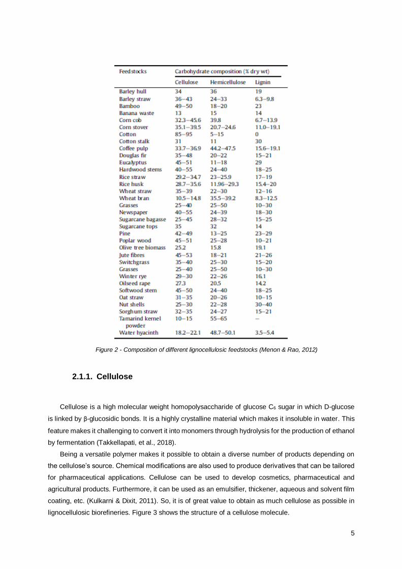

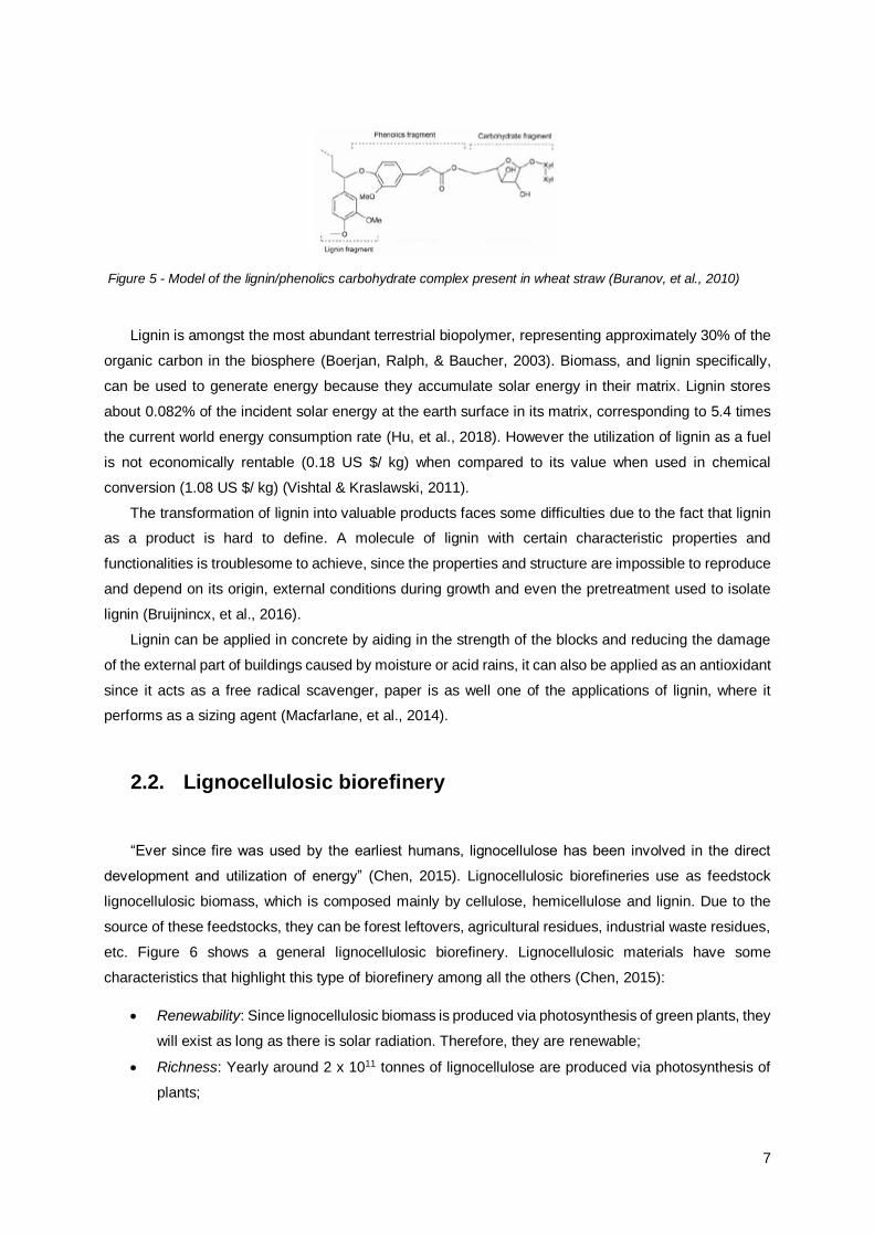


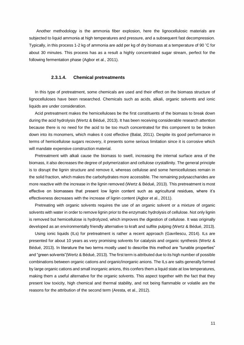


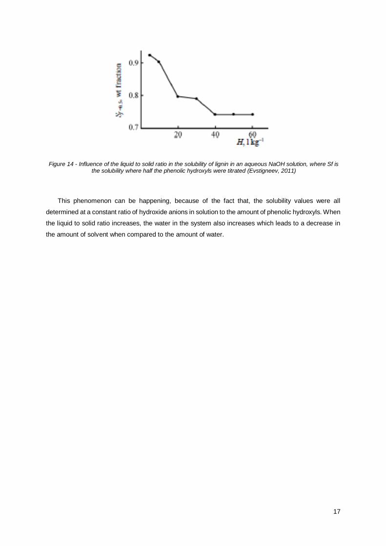


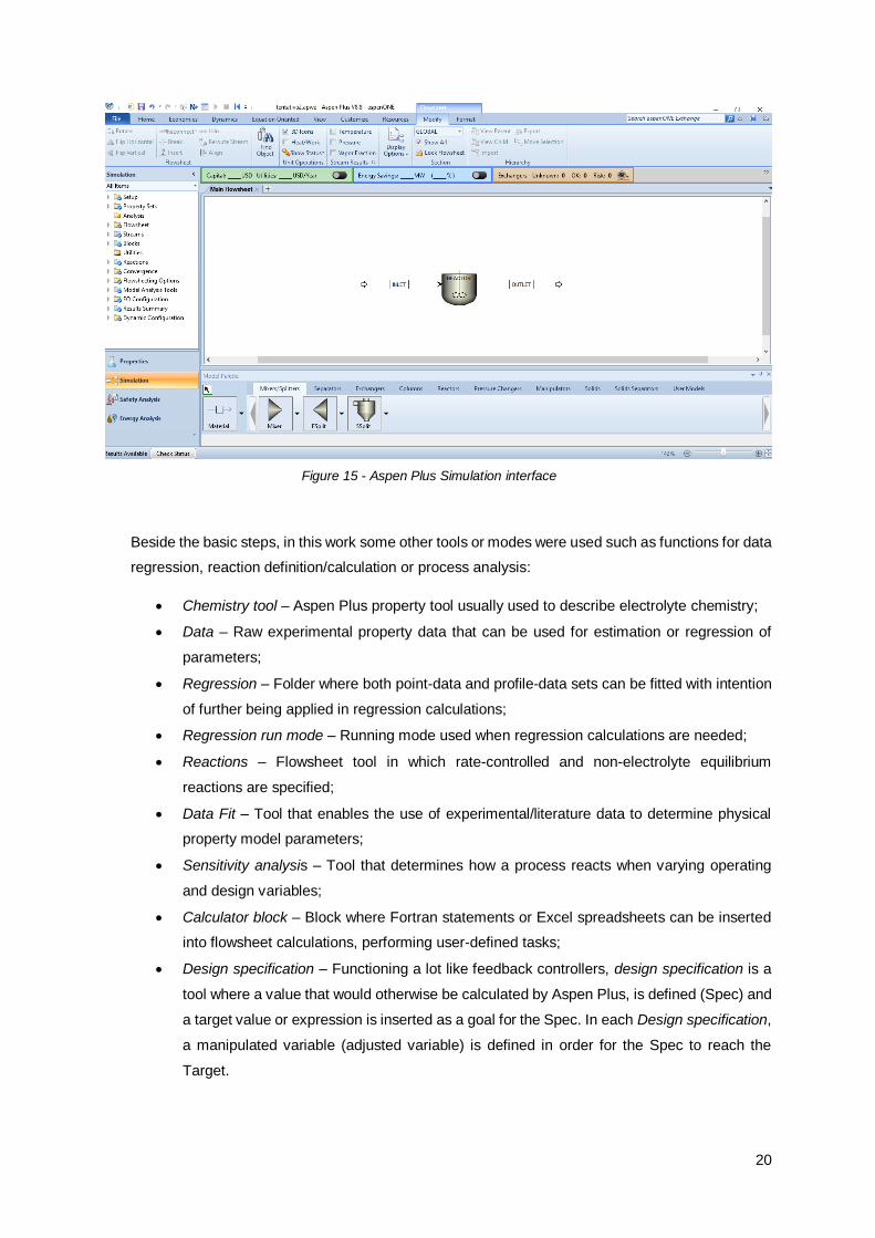

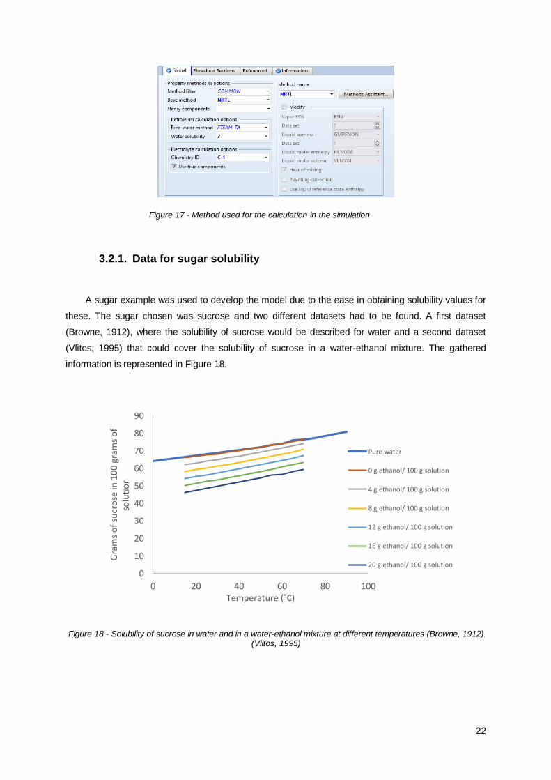


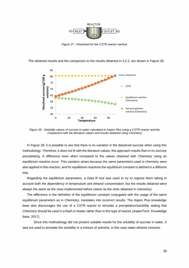

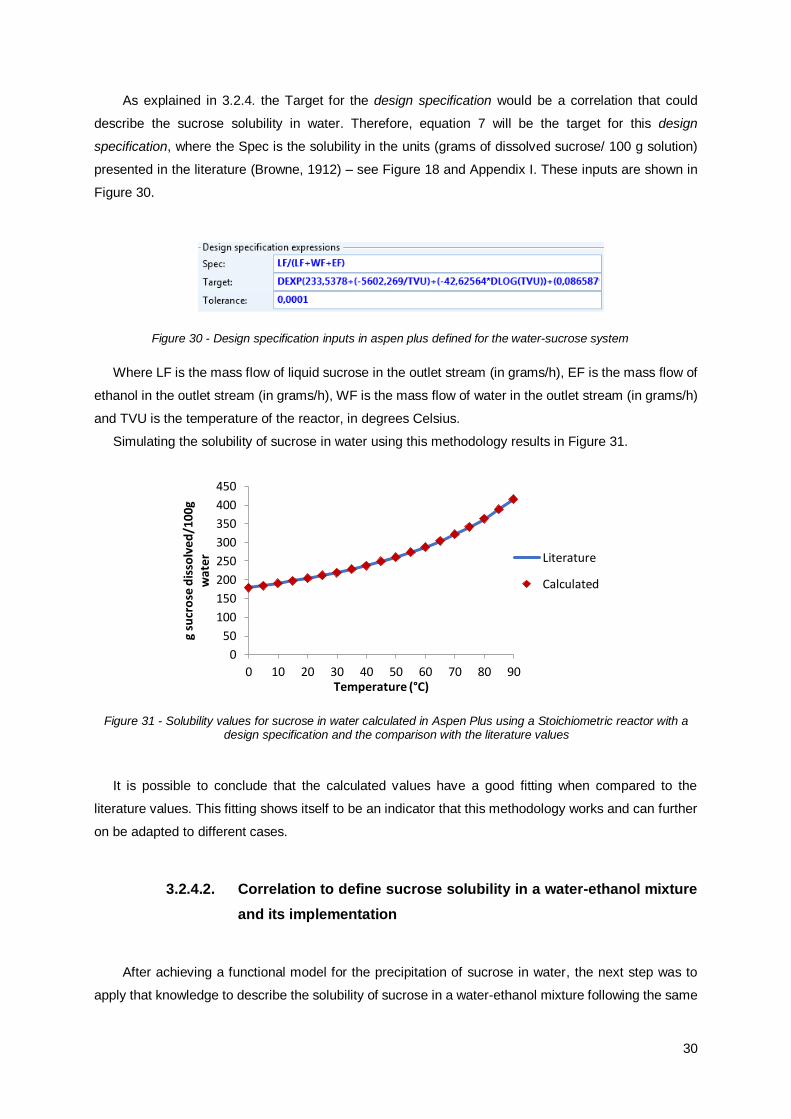
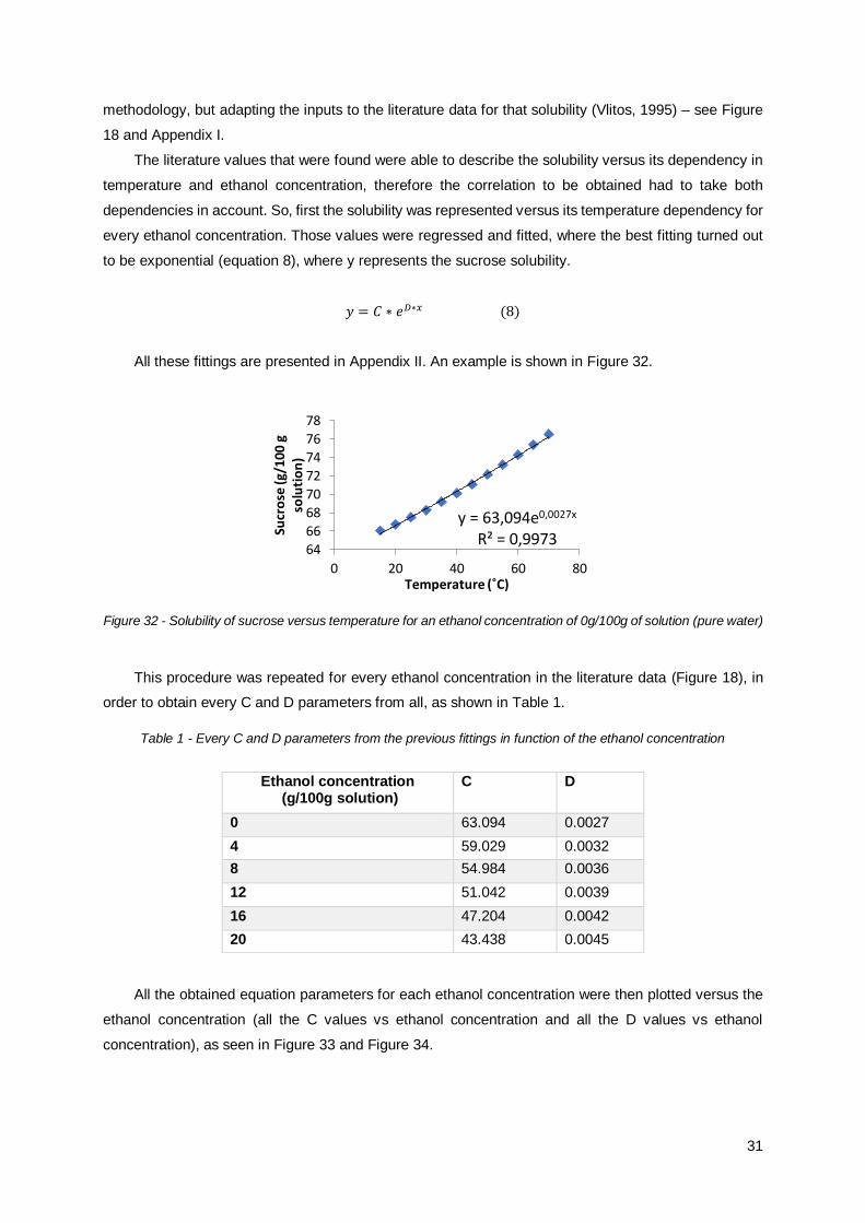
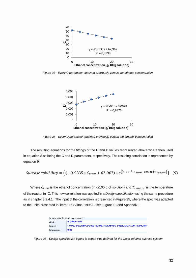


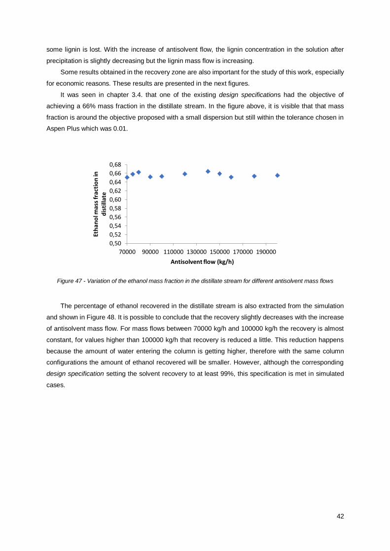


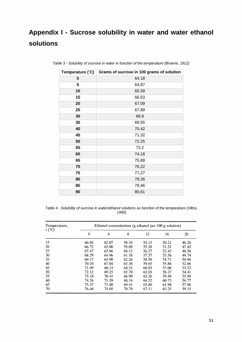


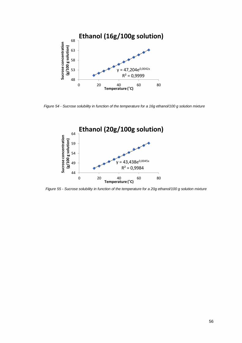
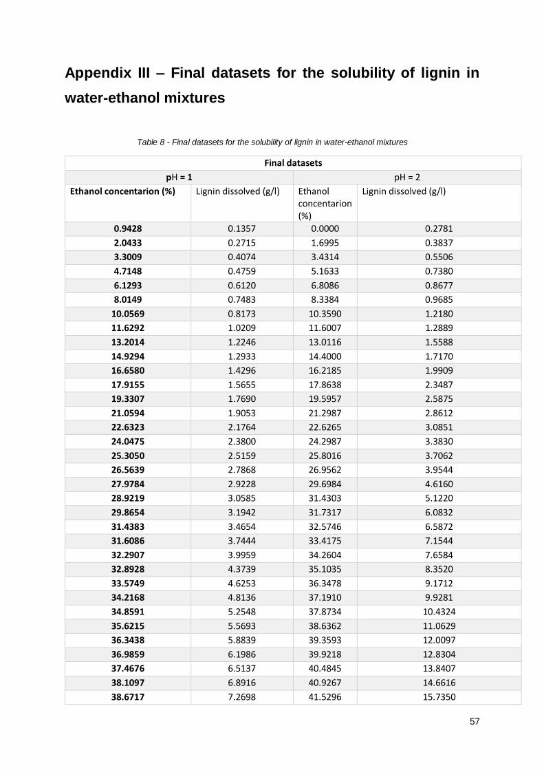


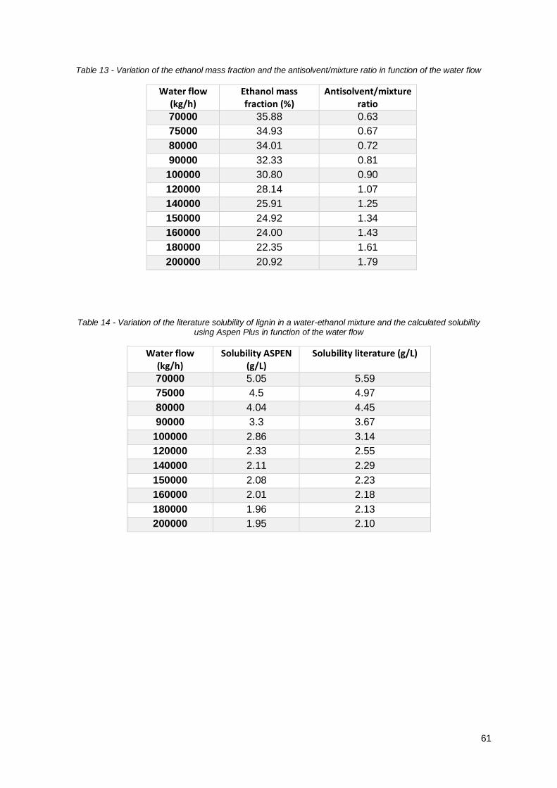


![Decrease of AOX with Various External Effluent Treatments · phite pulp mill [18]. An alternative lignin precipitation process is the lignin removal process (LRF’) [20] which uses](https://static.documents.pub/doc/80x56/5f4194da5d981c52071cc730/decrease-of-aox-with-various-external-effluent-treatments-phite-pulp-mill-18.jpg)


