Modeling and Simulation of Molecular Biology Systems using Petri

November 5, 2004 11:6 WSPC/185-JBCB 00076

Journal of Bioinformatics and Computational BiologyVol. 2, No. 4 (2004) 619–637c© Imperial College Press

MODELING AND SIMULATION OF MOLECULAR BIOLOGYSYSTEMS USING PETRI NETS: MODELING GOALS

OF VARIOUS APPROACHES

SIMON HARDY

Computer Engineering Department, Ecole Polytechnique de MontrealP.B. 6079, succ. Centre-Ville

Montreal, Quebec H3C 3A7, [email protected]

PIERRE N. ROBILLARD

[email protected]

Received 24 October 2003Revised 10 February 2004Accepted 29 March 2004

Petri nets are a discrete event simulation approach developed for system representation,in particular for their concurrency and synchronization properties. Various extensions tothe original theory of Petri nets have been used for modeling molecular biology systemsand metabolic networks. These extensions are stochastic, colored, hybrid and functional.This paper carries out an initial review of the various modeling approaches based onPetri net found in the literature, and of the biological systems that have been success-fully modeled with these approaches. Moreover, the modeling goals and possibilities ofqualitative analysis and system simulation of each approach are discussed.

Keywords: Biochemical pathways modeling; petri net; qualitative analysis; simulation.

1. Introduction

The completion of the human genome sequencing project, the rapid developmentof bioinformatics and the phenomenal accumulation of biological data have madethe understanding biological processes and cellular functions a growing researchinterest. This post-genomic wave is called “systems biology”, and with it has arisena greater interest in the modeling and simulation of biological systems.1 Manyformalisms from the fields of biology, mathematics and the computer sciences areused to integrate, represent and analyze the vast amount of biological data.

A traditional representation uses ordinary differential equations (ODEs) tomodel biological systems. It is widely used and many tools are based on this

619


620 S. Hardy & P. N. Robillard

approach.2 Appropriate for representing and simulating the kinetic equations ofbiochemical reactions, ODEs are mostly used to study the dynamics of a metabolicprocess. The software packages Gepasi3 and E-CELL4 have been developed to sup-port modeling with this analytical representation. Boolean logic and state machinesare also used for modeling biological systems. Even though boolean models aresimple representations, they can be used to express characteristics of biologicalphenomena.5 For example, a logic model of the Endo16 gene of Strongylocentrotuspurpuratus predicted an internal cis-regulatory switch.6 Stochastic models areanother approach used in molecular biology modeling. Processes like genetic expres-sion and regulation, signal transduction and cellular reproduction exhibit a stochas-tic behavior.7 A stochastic kinetic analysis of the phage λ lysis-lysogeny decisioncircuit resulted in statistics on regulatory outcomes.8 Many literature reviews pre-senting these modeling approaches and others have been published, and some booksintroducing the subject are available.9–12

Discrete event simulation is another interesting approach for molecular biologymodeling. Categorized in this last family of approaches, Petri nets can serve tomodel, analyze and simulate biological processes. The use of Petri nets in biologywas suggested for the first time by Reddy et al., who qualitatively analyzedmetabolic pathways.13 Since then, several types of biological processes have beenmodeled and simulated with Petri nets, mainly molecular biology systems, but alsoin epidemic and ecologic modeling.14–16 Peleg et al. assessed Petri nets and ten othertypes of model from the fields of software engineering, business and biology to eval-uate their appropriateness for representing and simulating biological processes.17

Their conclusions were that the combination of two of the assessed types of model,workflow and Petri net models, was the most suitable notation. Aptness of Petrinets for biological research is also demonstrated in recent articles.18–23 Furthermore,software tools for molecular biology modeling and simulation based on a Petri netarchitecture are being developed.24–26

Despite the various works with different Petri net approaches, Chen et al.emphasized that “they lack unity in their concepts, notations and terminologies.This makes it very difficult for new scientists to understand the potential appli-cations of Petri nets due to the various interpretations presented by differentauthors.”27 The aim of this paper is to analyze the modeling of biological sys-tem with the various types of Petri nets. For the complete methodology underlyingeach approach, the referenced articles should be consulted in their entirety. In thenext section, elements from Petri net theory and the earliest attempts at usingthem for modeling are introduced. Then, the modeling and simulation of biolog-ical process with stochastic, colored and hybrid Petri nets are presented and thecharacteristics of each approach are discussed. The glycolysis pathway, modeledwith three different types of Petri net, is illustrated. The formal definition of eachPetri net type and the definitions of some of their properties are included witheach presentation. Petri nets have also been used to analyze metabolic pathway


Modeling and Simulation of Molecular Biology Systems Using Petri Nets 621

databases.28 In this kind of application, Petri nets are useful for comparing datafrom various sources, but this is not within the scope of this paper.

2. Elements of Petri Net Theory and the Earliest Attemptsat Biological Modeling

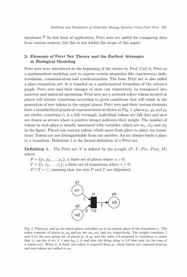
Petri nets were introduced at the beginning of the sixties by Prof. Carl A. Petri asa mathematical modeling tool to express system properties like concurrency, inde-terminism, communication and synchronization. The basic Petri net is also calleda place/transition net. It is founded on a mathematical formalism of the orientedgraph. Petri nets and their changes of state can respectively be transposed intomatrices and matricial operations. Petri nets are a network where tokens located inplaces will initiate transitions according to given conditions that will result in thegeneration of new tokens in the output places. Petri nets and their various elementshave a standardized graphical representation as shown in Fig. 1: places p1, p2 and p3

are circles, transition t1 is a full rectangle, individual tokens are full dots and arcsare drawn as arrows where a positive integer indicates their weight. The number oftokens in each place is usually associated with variables, which are m1, m2 and m3

in the figure. Places can contain tokens which move from place to place via transi-tions. Tokens are not distinguishable from one another. An arc always binds a placeto a transition. Definition 1 is the formal definition of a Petri net.

Definition 1. The Petri net N is defined by the n-tuple (P , T , Pre, Post, M)where:

P = {p1, p2, . . . , pu}, a finite set of places where u > 0;T = {t1, t2, . . . , tv}, a finite set of transitions where v > 0;P ∩ T = �, meaning that the sets P and T are disjointed;

Fig. 1. Places p1 and p2 are input places and place p3 is an output place of the transition t1. Thetoken contents of places p1, p2 and p3 are m1, m2 and m3 respectively. The weight constants 1and 3 on the arcs going out of places p1 et p2 and the value 1.0 attached to transition t1 meanthat t1 can fire if m1 ≥ 1 and m2 ≥ 3, and that the firing delay is 1.0 time unit (in the case ofa timed net). When t1 is fired, one token is removed from p1, three tokens are removed from p2

and two tokens are added to p3.



Pre = P × T → N, is the input incidence mapping (weights of the arcs goingfrom places to transitions) and where N is the set of natural numbers;

Post = P × T → N, is the output incidence mapping (weights of the arcs goingfrom transitions to places);

M = P → N, is the marking of the net which is a vector of u components(m1, m2, . . . , mu), where mi is the number of tokens contained in the place pi.M0 is the initial marking.

The marking M of the network gives the state of the Petri net. It is a vec-tor indicating the number of tokens M(p) at each place p. When a transition isfired, there is a change in the state of the net, and consequently a modification ofthe marking. A firing can occur when all the input places of a transition containthe minimal number of tokens defined by the Pre relation. In other words, when thenumber of tokens of all input places is greater than or equal to the weight of thearc linking them to a transition, this transition can fire. Then, the tokens are con-sumed by the transition and withdrawn from the input places, just as other tokensare created and added to the output places of the same transition. The numberof tokens created is specified by the Post relation. Figure 1 illustrates how a Petrinet transition works. For a more formal and complete coverage of traditional Petrinets and an analysis of their structural properties, consult Reisig’s introduction onthe subject.29 Many extensions have been added to the initial model, the purposeof which is to transform models into a more compact form, to elevate the abstrac-tion level or to give Petri nets new capabilities. Some of them have been used formodeling and simulation in biology, and these will be briefly presented in the fol-lowing sections. The similarities between modeling in molecular biology and Petrinet theory are thoroughly discussed.23

Traditional Petri nets were originally suggested for biological pathway model-ing by Reddy et al., and the bridging of molecular species and chemical reactionswith Petri net places and transitions was achieved for the first time by them.13

The association of places with molecular species and transitions with chemicalreactions is used for all types of Petri net model presented in this review. However,special situations necessitate more than one place for one species, for example,when distinguishing between an enzyme in an activated or a deactivated state, or ametabolite in various sites of the cell. The number of tokens indicates the quantityof substance and it corresponds to a predefined measure unit according to the scaleof the model, such as the exact number of molecules, mole, millimole, etc. Reddydemonstrated that the Petri net approach was an appropriate tool for a preliminaryqualitative analysis of biopathways. Behavioral and structural properties of Petrinets, like liveness, boundedness and invariants were used to identify some charac-teristics of models (see Definitions 2 to 6). This analysis approach was applied tothe erythrocyte pentose phosphate pathway and to the main glycolytic pathway(see Fig. 2 for model and Tables 1 and 2 for symbols definition).30 The analysisof these pathways showed boundaries for certain molecular species, conservation



Fig. 2. The Petri net model of the combined metabolism of the glycolytic and pentose phosphatepathways of an erythrocyte cell transforming glucose into lactate (pentose phosphate pathway isabstracted by transition t13). Places labeled with an asterisk are, in fact, one place only, whichhas been divided for reasons of clarity. ATP, for example, has only one place. See Tables 1 and 2for elements definition. Model inspired after Fig. 8 from Reddy et al .30

Table 1. Mapping between metabolites in the pathway and places in the Petri netmodels of Figs. 2, 3 and 6.

Metabolite/Compound

Marking Variable AssociatedAbbreviation to Concentration Name

Gluc m1 GlucoseG6P m2 Glucose-6-phosphateF6P m3 Fructose-6-phosphateFBP m4 Fructose biphosphateDHAP m5 Dihydroxyacetone phosphateGAP m6 Glyceraldehyde-3-phosphate1,3-BPG m7 1,3-Biphosphoglycerate3PG m8 3-Phosphoglycerate2PG m9 2-PhosphoglyceratePEP m10 PhosphoenolpyruvatePyr m11 PyruvateLac m12 LactateATP m13 Adenosine triphosphateADP m14 Adenosine diphosphateNAD+ m15 Nicotinamide adenine dinucleotide,

oxidized formNADH m16 Nicotinamide adenine dinucleotide,

reduced formPi m17 Orthophosphate, ionic form

properties, regenerative reactions and situations leading to a deadlocking of thesystem.

Definition 2. Reachability. A marking M is reachable if it can be reached fromthe current marking Mi in a finite firing sequence.



Table 2. Mapping between reactions in the pathway andtransitions in the Petri net models of Figs. 2, 3 and 6.

Index Enzyme/Reaction

t1 Hexokinaset2 Phosphoglucose isomerase (forward reaction)t3 Phosphofructokinaset4 Aldolaset5 Triosephosphate isomerase (forward reaction)t6 Triosephosphate isomerase (reverse reaction)t7 Glyceraldehyde-3-phosphate dehydrogenaset8 Phosphoglycerate kinaset9 Phosphoglycerate mutaset10 Enolaset11 Pyruvate kinaset12 Lactate dehydrogenaset13 Pentose phosphate pathway abstractiont14 Phosphoglucose isomerase (reverse reaction)

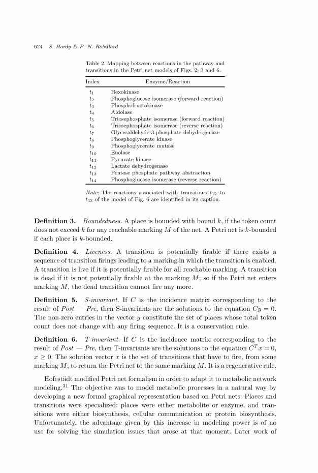
Note: The reactions associated with transitions t12 tot43 of the model of Fig. 6 are identified in its caption.

Definition 3. Boundedness. A place is bounded with bound k, if the token countdoes not exceed k for any reachable marking M of the net. A Petri net is k-boundedif each place is k-bounded.

Definition 4. Liveness. A transition is potentially firable if there exists asequence of transition firings leading to a marking in which the transition is enabled.A transition is live if it is potentially firable for all reachable marking. A transitionis dead if it is not potentially firable at the marking M ; so if the Petri net entersmarking M , the dead transition cannot fire any more.

Definition 5. S-invariant. If C is the incidence matrix corresponding to theresult of Post — Pre, then S-invariants are the solutions to the equation Cy = 0.The non-zero entries in the vector y constitute the set of places whose total tokencount does not change with any firing sequence. It is a conservation rule.

Definition 6. T-invariant. If C is the incidence matrix corresponding to theresult of Post — Pre, then T-invariants are the solutions to the equation CT x = 0,x ≥ 0. The solution vector x is the set of transitions that have to fire, from somemarking M , to return the Petri net to the same marking M . It is a regenerative rule.

Hofestadt modified Petri net formalism in order to adapt it to metabolic networkmodeling.31 The objective was to model metabolic processes in a natural way bydeveloping a new formal graphical representation based on Petri nets. Places andtransitions were specialized: places were either metabolite or enzyme, and tran-sitions were either biosynthesis, cellular communication or protein biosynthesis.Unfortunately, the advantage given by this increase in modeling power is of nouse for solving the simulation issues that arose at that moment. Later work of



Hofestadt and Thelen suggested a solution to this problem: the application of aPetri net extension corresponding more to the biological context.32 This extensionis the self-modified Petri net, first defined by Valk and now known as the functionalPetri net (see Definition 7).33 The main feature of this augmented formalism isthe possibility of assigning to Petri net arcs an equation using marking variablesinstead of a positive integer. The result is that network marking dynamically mod-ifies the weight of the arcs. In the case of a biochemical process model, this featureis particularly useful for simulating the influence of the variation in concentrationon the kinetic rate of biocatalytic reactions. In other words, concentrations, rep-resented by the number of tokens in the net, are variables for the functions thatdefine the weight of the arcs. Thus, the reaction rate of a transition is modifiedaccording to the concentration of the various substances involved. Hofestadt andThelen suggested that quantitative simulations with self-modified Petri nets wouldhelp detect metabolic bottlenecks in some defective processes.

Definition 7. The functional Petri net N is defined by the n-tuple (P , T , Pre,Post, V , M) where:

(P , T , Pre, Post, M) is a Petri net as described in Definition 1;V = {ga(m1, . . . , mu), a ∈ Pre∪Post | g : p1 × · · · × pu → N}, a set of functions

assigned to arcs of the net using its marking (m1, . . . , mu) as parameters.

3. Stochastic Petri Nets

The random nature of molecular interactions at low concentration has beenobserved in several experiments. However, the Kolmogorov equations of the stochas-tic model corresponding to a biological system rapidly become impossible to solveanalytically. Goss and Peccoud used stochastic Petri nets (SPN)34 as a tool forbiological modeling of stochastic models.7 They implied that the Petri net formal-ism and its modeling power can reduce model implementation delays. With theirmodel, they successfully analyzed the stabilizing effect of the ROM protein on thegenetic network controlling the replication of ColEl plasmid replication.35 Morerecently, the response of transcription factor σ32 to a heat shock and the intra-cellular kinetics of a viral invasion have been studied through simulation of SPNmodels.36,37

In the SPN model of a system composed of molecular interactions, each placecorresponds to a particular molecular species. Tokens represent molecules and tran-sitions between places are chemical reactions involving reactants (input places) andproducts (output places). At any time, the marking of the system indicates thenumber of molecules of each species involved. The values of arcs originating frominput places and ending at output places are the equivalent of stochiometric coef-ficients. As in traditional place/transition nets, if the number of tokens at inputplaces is higher than the weight of all the input arcs of a transition, this transi-tion can fire. In molecular terms, the firing of a transition means that a chemical



reaction is occurring. The particularity of SPN is that the firing of a transitionis not instantaneous. There is a delay following a probabilistic distribution, thusthe delay is a random variable (see Definition 8). In SPN biological models, thisdelay is interpreted as the reaction rate, and it is given by the weight function ofthe corresponding transition. The delay mean time is obtained by the transitionreaction rate, which is a function of a stochastic rate constant and the quantityof each molecular species involved as a reactant or a catalyst. This constant takesinto account volume, temperature, pH and other environmental factors. It is alsorelated to the deterministic rate of the reaction. Several types of SPN exist, but,in the type discussed here, the same type that is used by Goss and Peccoud formodeling a biological process, the weight function will take into account the mark-ing of the net in order to correctly calculate reaction rates. When the number ofmolecules is sufficiently large, the stochastic constant of the reaction rate is equalto the deterministic rate.

Definition 8. The stochastic Petri net N is defined by the n-tuple (P, T, Pre,

Post, F, λ, M) where:(P, T, Pre, Post, M) is a Petri net as described in Definition 1;F = {Ft, t ∈ T | Ft: [0,∞) → [0, 1]}, a set of probability density functions for

the net firing delays. Their average is 1 and they are independent of the marking;λ = {λt, t ∈ T | λt: N → R

+}, a set of firing rates, which are function of themarking (a set of natural integers) and where each element is associated with atransition t. This rate, a positive real number from the set R

+, is used to calculatethe probability density function for the transition t.

Stochastic models are applicable when molecules are considered as a discreteamount. Then, a deterministic change in concentrations, quantified by reactionkinetic rates of the incessant flux of transformation of reactants in products,becomes a random event where reactions are ruled by probabilistic laws. SPN canhelp build these models from their reaction equations and simulate them. It conse-quently becomes possible to study a system with the simulation results.

The software Mobius (or UltraSAN in its earlier version) has been used for allthe systems modeled with SPN mentioned in this section.38 This SPN simulationtool — not exclusive to biology — also has a model numerical resolution option.With this tool, the molecular species distribution can be studied and the occurrenceprobability of certain events can be calculated. For example, in the analysis of thestabilizing effect of the ROM protein on a genetic network, the probability that acell will divide without having replicated its plasmid was estimated.

4. Colored Petri Nets

The differentiation between categories of tokens when modeling large systems withPetri nets was considered in order to reduce the size of models. Thus, Petri netswere enhanced with this new feature by adding colors. The resulting high-level



net, colored Petri net (CPN), is composed of tokens identified by a color (seeDefinition 9). With this augmentation of the formalism, it is possible to represent,in the same model, different dynamic behaviors modeled by different token colors.39

Two research teams modeled and simulated biological processes with CPN. In allprojects, Design/CPN software, consisting of a set of edition and simulation toolsfor CPN, has been used.40 However, each team had a different modeling goal andthe conceptual meaning of the token colors was not the same.

Definition 9. The colored Petri net N is defined by the n-tuple (P, T, Pre, Post,

C, M) where:(P, T, Pre, Post, M) is a Petri net as described in Definition 1 and the tokens

of M are identified by a color;C = {C1, C2, . . .}, a set of colors. The incidence mappings Pre and Post are

functions of the token colors.

Genrich et al. modeled an enzymatic reaction with a colored Petri nettransition.41 This transition is connected to places representing substrates likere-actant, product, enzyme and inhibitor. In this model, tokens are identifiedby two colors, one associated with the substance name and the other withits concentration. The CPN used for this modeling also has functional fea-tures because an execution model is called upon, after every firing of thetransition, to calculate and modify substrate concentration. These reactionrate calculations are performed according to the Michaelis–Menten biochemi-cal equation, augmented by an additional term for the free reaction energy.The specific constants associated with each enzyme needed for these calcu-lations are extracted from the BRENDA biochemical database.42 This tran-sition is, in fact, a sub-model integrated into the glycolysis and citric acidmetabolic models. A chain of enzymatic reactions constitutes the metabolicnetwork to be quantitatively simulated. Another interesting part of the Gen-rich et al. paper is to propose rules for automatic pathway identification fromdatabases, after which the pathways are modeled as Petri nets for simulationpurposes.

Although the CPN was used in their work to model a metabolic system, Heiner,Koch and Voss proceeded differently to accomplish a qualitative analysis of steadystates in pathways.43,22 The objectives of this approach are compatible with thework of Reddy, but the modeling power and the communication capacity of themodel are enhanced by the addition of colors. They refined the initial Reddy modelof glycolysis and pentose phosphate pathways in an erythrocyte cell by the inclusionof reversible reactions and flux modes (see Fig. 3 for model). Unlike to Genrich, theintention in using colors was to separate branches of a metabolic pathway and todifferentiate molecules of the same species (thus, tokens of the same place) accordingto their origin and destination reaction. The analysis of the invariants of the CPNmodel found a preservation law for the amounts of all metabolites in the systemand confirmed regenerative reactions and their partial order.



Fig. 3. Colored Petri net model of the glycolysis and pentose phosphate pathways of an erythrocytecell. The colors used in this model are C, D and H′. The variable X means any color. Three fluxmodes are represented in the original model. The first mode is glycolysis, associated with theguard [X <> C] of t13, which means that tokens of color C cannot travel through the pentosephosphate pathway. The two other modes are combined in the pentose phosphate pathway (alldetails are not shown), one of them is associated with the guard [X <> H′]. Model inspired afterFig. 3 from Heiner et al .43

5. Hybrid Petri Nets and Supplementary Extensions

An intuitive way for representing a molecular species concentration is with tokensof a continuous nature instead of a discrete nature. The hybrid Petri net (HPN)offers this possibility with a new continuous type of places and transitions (seeDefinition 5).44 In HPN, discrete places and transitions, with their number of tokensrepresented by integers and their possible firing delay, are unchanged. But, in thenew continuous places, tokens are replaced by a non-negative real number calleda mark, and a variable called speed is assigned to the new continuous transitions.The continuous transition speed is a rate of quantity transformation from inputplaces to output places. Thus, the modeling of metabolic reactions and geneticregulation, usually performed with ODEs, can now be accomplished with hybridPetri nets. Figure 4 explains how a continuous HPN transition operates, and Fig. 5shows the HPN elements graphically. Matsuno et al.45 and Chen and Hofestadt18

have demonstrated the feasibility of modeling biological systems with HPN.

Definition 10. The hybrid Petri net N is defined by the n-tuple (P, T, Pre,

Post, h, M) where:(P, T, Pre, Post, M) is a Petri net as described in Definition 1, where M is

a combination of integers for the number of tokens in discrete places and of realnumbers for the mark of continuous places;

h: P ∪ T → {D, C}, called a hybrid function, indicates for each place andtransition, if it is discrete (h(pi) = D and h(tj) = D) or continuous (h(pk) = C

and h(t1) = C);



Fig. 4. Places p1, p2 and p3 are continuous places having content m1, m2 and m3 respectively.The function m1 − m2/2 is assigned to the continuous transition t1 as its firing speed, t1 can befired if m1 > 0 and m2 > 0. The contents of p1 and p2 are consumed with the speed m1 − m2/2,and the content of p3 increases with the same speed when the transition t1 is fired.

Fig. 5. Graphical representations of the elements of hybrid Petri nets.

A delay dt is assigned to all discrete transitions and a speed vt is assigned to allcontinuous transitions.

Matsuno et al. modeled the genetic switching mechanism of the λ phage withHPN45 by using the Visual Object Net++ tool.46 Part of their work demonstratedthat the HPN approach constitutes a more intuitive modeling tool than the ODE,because of its graphical notation as much as for its power as a simulation tool.The variations in expressed protein concentration, resulting from the simulations,correspond to the biological data on that system.

To be able to adapt the HPN modeling approach to biological processesmore accurately, functional Petri net properties have been added to create anew extension: the hybrid functional Petri net (HFPN).24 This twinning allowsa dynamic adaptation during the execution of the Petri net like that in the Genrichet al. work.41 The attribution of a value to the net arcs makes it possible to modelbiochemical reaction rate equations like the Michaelis–Menten equation. Moreover,two new arc types, different from “normal” arcs, are included in the HFPN to modelbiological aspects. Firstly, inhibitory arcs model the inhibition function of moleculesin some reactions. An inhibitory arc with weight r enables the transition to fireonly if the content of the place at the source of the arc is less than or equal to r.



Secondly, test arcs verify the presence of content at its source place when the relatedtransition fires without consuming anything. Unlike inhibitory arcs, some content isnecessary in a place connected with a test arc to a transition about to fire. With theinhibitory arc, the repressing function of an operator on gene transcription can berepresented. With the test arc, the action of an enzyme in a metabolic reaction,where the enzyme is required but not consumed by the reaction, can be modeled.From the HFPN architecture, the Matsuno team has developed biosimulation soft-ware for biologists called Genomic Object Net (GON).25,26,47

Many biological processes and systems have already been modeled and simulatedusing HFPN. Some processes are related to genetic regulation: the λ phage geneticcontrol mechanism,45 circadian rhythms in Drosophila19 and the control mecha-nism of the lac operon of E. coli.20 Others are metabolic networks: the glycolyticpathway32 (see Fig. 6) and the urea cycle.18 The transduction signal system ofapoptosis induced by the Fas ligand was also modeled with HFPN.19 The patternformation by a multicellular system due to interactions between cells with Delta-Notch signaling was simulated.48 In this last experiment, a cellular boundary forma-tion in Drosophila and other abnormal patterns could be analyzed with simulationresults, corroborating observations from laboratory experiments.

The scientists who originated the HFPN architecture are continuing its elabo-ration by planning the incorporation of extensions to enhance its modeling powerand simulation precision.19 To achieve this, more complex information like the

Fig. 6. Hybrid functional Petri net model of the glycolytic pathway and lac operongene regulatory mechanism. Transitions t12–t23 are the natural degradation of substratesand their firing speed is given by the formula mX/10000 where X = 1, 2, . . . , 10, 12, 13.Production rate of enzymes (t24, t26, . . . , t42) has a speed set to 1 and their degradation rate(t25, t27, . . . , t43) has a speed given by the formula (enzyme concentration)/10. The reactions inthe main pathway (t1, t2, . . . , t11) have the Michaelis–Menton equation for speed: VmaxmX

Km+mXwhere

X = 1, 2, . . . , 10, Vmax is the maximum reaction speed and Km is a Michaelis constant. Modelinspired after Fig. 9 of Ref. 20.



localization of biological objects or intercellular interactions at the molecular levelmust be incorporated into the models. One of these extensions makes it possible fora Petri net place to have various data types, like integers or real numbers, vectorsand strings. Also, a conversion module implementing the procedure will be capableof converting biological models represented with ODEs in the E-CELL softwareformat to HFPN models.49

6. Discussion

To make the modeling power of Petri nets richer and to adapt them to diverseproblems, several extensions have been added to Professor Petri’s theory. However,enhancements given by the extensions presented in this review do not offer thesame modeling and simulation possibilities. Colored Petri nets (CPN) were createdto diminish model size and so allow the models to manage more information withoutrendering its structure too complex. Stochastic Petri nets (SPN) are a specializedmember of the timed Petri net family where firing delays are random variables.The need to represent discrete and continuous quantities in the same model moti-vated the development of hybrid Petri nets. Finally, the dynamic modification of arcweight through net marking is possible with functional Petri nets. Other extensionswere developed to solve other problems. With the variety of Petri net types avail-able, the context of use of the various extensions for biological process modelingand simulation can be called into question.

To analyze each approach and its biological modeling possibilities, it is pertinentto recall the compromise discussed by Reddy et al. between the modeling andsimulation power and the decision-making power of Petri net.30 According to thiscompromise, the addition of modeling power to a Petri net with extensions willdecrease its analytic capabilities. Indeed, augmenting modeling power amplifies thecomplexity of the determination of some properties, even to the point of indecision.For example, inhibitor arcs expand the richness of concepts expressed by a model,but greatly complicate its mathematical analysis. Thus, it is important to choosethe Petri net extension that will be used for modeling judiciously, in accordancewith the objectives to be attained.

In the literature, there are two categories of goals of Petri net biologicalmodeling: qualitative and quantitative analysis. One can either learn more aboutthe properties of the system under study with a qualitative approach or study thesystem dynamics with simulation. When one wants to analyze a complex system ofbiochemical reactions, for example by identifying invariants, the presence of bound-aries or the liveness in the system model, the Petri net extension chosen must enablethose properties to be determined. By contrast, one may want to study the model’sbehavior by simulating it and thus obtain concentration graphs, and/or observethe achievability of a steady state, without any concern for property decidability.In that case, modeling power is more important. Thus, it is possible to identifymodeling goals for each Petri net extension (see Table 3).



Table 3. Biological modeling goals of Petri net extensions.

Petri Net AvailableExtension Modeling Goal Analysis Type Process Type Software References

Colored Analysis of Qualitative Metabolic Design/CPN 22, 42, 44biologicalsystemproperties

Stochastic Simulation of Quantitative Any biological Mobius 7, 36, 37, 38biological stochasticsystems processwith lowconcentrations

Hybrid Simulation of Quantitative Metabolic, Genomic 18, 19, 24, 25,functional biological Regulatory Object Net 26, 46, 49

systems networks, Signaltransduction

As was the case for the earliest modeling attempts with Petri net by Reddy et al.,where a qualitative analysis was performed using place/transition nets, CPN cangive some insights into a biological system.43 Thus, a rigorous preliminary analysiscan guide the elaboration of experiments when quantitative data is missing. Tokencolor does not reduce the decidability power of Petri nets because it is alwayspossible to convert each CPN mode into a traditional net. One advantage of usingCPN is the possibility of discriminating metabolites on the basis of their chain ofreactions in a model. However, the size of the model must not exceed a certain limitbecause if the model complexity is too great, the state space will explode and itscomplete exploration and analysis will be impossible. Consequently, the analysis ofcomplex systems is still a difficult task. Until now, this method has only been usedon classic metabolic systems (like the Krebs cycle or glycolysis) to demonstrateits potential, but has also been incorporated in algorithms to find new metabolicpathways between two compounds.28 Little information is needed to perform aqualitative analysis: the stoichiometry and the reversibility of the system reactions.

Hybrid and stochastic net attributes are intended for simulation, and tokenactivity in the model is the main aspect considered in reproducing the behaviorof a system. Wanting to model a system in order to quantitatively simulate it isin accordance with the modeling goals of Hofestadt and Thelen.32 The criterion ofchoice between the stochastic and the hybrid extensions is the nature of the systemto be modeled. If, for example, a model deals with a small number of molecules,such that their individuality has to be taken into account, its stochastic naturehas to be represented and SPN are appropriate. By contrast, for models where thenumber of molecules is high enough to be represented in a satisfying way as a con-tinuous quantity or as a concentration, HPN is the appropriate modeling approach.It is interesting to note, however, that, if the discrete transition delay in HPN is



modified to become a random variable, then it is possible to fuse HPN with SPN.Matsuno et al. mentioned that their architecture could be easily modified to allowthis blending.45 It is also important to recall that the twinning of the functional andhybrid extensions, as in the HFPN, facilitates the modeling of metabolic reactions.

To accomplish a quantitative analysis of a biological system, kinetic parameterslike reaction rates have to be available. This kind of analysis provides means to testnew hypothesis and to evaluate the impact of the variation of conditions in which asystem evolves. It has proven its usefulness in several biology research projects.As mentioned above, the stabilizing effect of the ROM protein on the geneticnetwork controlling the replication of ColE1 plasmid replication was successfullyanalyzed with a SPN model35 and a cellular boundary formation in Drosophilacould be analyzed with simulation results of a HFPN model, corroborating obser-vations from laboratory experiments.48

The work of Genrich et al.41 is an exception to the classification shown inTable 3. In their model, the color of the tokens is associated with the concentrationof the molecular species in order to make a quantitative analysis. This demonstratesthat the classification is not absolute. However, in addition to the colored extension,the Petri net type used in that model also includes an executable component whichis called upon at every transition firing to calculate the concentration variationsaccording to the Michaelis–Menten equation. Despite the validity of this approach,it is less intuitive and harder to implement than an approach using HFPN.

Using the Petri net for biological modeling offers many advantages. First, twoPetri net properties, identified by Reddy et al., are pertinent to the modeling ofbiochemical systems: extendibility and abstraction.30 These two features are relatedto model hierarchization. Extendibility is the property of adding new sections to anet — for example, when supplementary information becomes available to completea model, or when one wants to combine two complementary models — withouthaving to considerably modify the structure of the resulting model. Abstractionis the property of neglecting the modeling of some aspects which do not concernthe system under study by representing the sub-model by a transition. An exampleof abstraction is the transition t13 of the Figs. 2 and 3 representing the pentosephosphate pathway.

Second, many theoretical elements of Petri nets with a mathematical basis areuseful as a preliminary analysis tool for biological pathways. Zevedei–Oancea andSchuster thoroughly discuss this.23 Oliveira et al. developed and defined rigorouslya computational approach based on Petri nets to identify interesting sub-circuitpathways in biochemical networks and applied their methodology to the Krebscycle.50,21 Petri net invariants can be associated with flux modes and conservationrelations. Furthermore, special sets of places known as siphons and traps can beidentified. The places constituting a siphon stay empty once they have no tokens.At the other extreme, places forming a trap cannot lose one token when theyreach a certain marking. Traps and siphons are of interest in biochemical modeling



because these notions can be associated with the storage and consumption of systemresources. Finally, the liveness of a net or its deadlocked condition are also propertieswhich provide information about the biological system.

Third, biologists can easily model a biological system with the Petri net, andstudy it with the simulation capabilities of Petri net tools. The graphical aspects ofthe Petri net are quite similar to biochemical network representation, and this givessuperior communication ability to models and facilitates their design. Moreover,the Petri net is readily comprehensible and necessitates little related knowledgeon the part of biologists. Its mathematical basis makes it possible to accomplishcomplex simulations and to visualize results. The development of software basedon the Petri net and specific to biology, like the Genomic Object Net tool,25,26,47

and the proposal of a data exchange format for models, the “Biology Petri NetMarkup Language” (BioPNML)27,51 leave few obstacles for the adoption of a Petrinet approach by biologists. A powerful analysis and simulation environment can beimplemented from this modeling technique to study hundreds, even thousands, ofinterconnections formed by the various genetic and metabolic networks in the cell.

Several types of formal representation other than Petri nets are required tomodel biological processes. It was demonstrated that ordinary differential equationscan be substituted by HFPN, but other biological phenomena involving spatialmodeling, like diffusion, or molecular motions modeling, like molecular motors, donot have an equivalent in Petri net modeling. Because of the potential extensibilityof Petri net formalism, it is possible to think that scientists will go beyond thesemodeling limits. Thus, we could also say that these biological phenomena do nothave an equivalent in Petri net modeling yet.

7. Conclusion

In this paper, analysis, modeling and simulation of molecular biology systems usingPetri nets have been presented and an overview of various approaches using colored,stochastic, hybrid and functional Petri nets was made. The modeling goal of eachapproach was identified, thus providing a starting point to interested new users.

Petri net is a formalism with many advantages for biologists. It has analyticaland simulation capabilities which provide means to test hypotheses and gatherinformation that might help the elaboration of experiments. As we learn more aboutmetabolic pathways, gene regulatory networks and signalling pathways, powerfulmodeling tools like Petri net will be needed to understand the complexity of livingsystems.

Acknowledgments

We would like to thank Prof. Hanifa Boucheneb for her insightful comments and thetwo anonymous reviewers for their useful remarks about this article. This work wassupported in part by NSERC grant A-0141 and a Canada Graduate Scholarship.



References

1. Kitano H, Computational systems biology, Nature 420:206–210, 2002.2. Heinrich R, Schuster S, The modelling of metabolic systems. Structure, control and

optimality, Biosystems 47:61–77, 1998.3. Mendes P, GEPASI: a software package for modelling the dynamics, steady states and

control of biochemical and other systems, Comput Appl Biosci 9(5):563–571, 1993.4. Tomita M, Hashimoto K, Tabahaski K, Shimizu T, Matsuzaki Y, Miyoshi F, Saito K,

Tanida S, Yugi K, Venter JC, Hutchison C, E-CELL: Software for whole cell simula-tion, Bioinformatics 15:72–84, 1999.

5. Kauffman SA, The Origins of Order: Self-Organization and Selection in Evolution,Oxford University Press, New York, 1993.

6. Yuh CH, Bolouri H, Davidson EH, Cis-regulatory logic in the endo 16 gene:switching from a specification to a differentiation mode of control, Development128:617–629, 2001.

7. Goss PJE, Peccoud J, Quantitative modeling of stochastic systems in molecularbiology by using stochastic Petri nets, Proc Natl Acad Sci USA 95:6750–6755, 1998.

8. Arkin A, Ross J, McAdams HH, Stochastic kinetic analysis of developmental path-way bifurcation in phage lambda-infected Escherichia coli cells, Genetics 149:1633–1648, 1998.

9. de Jong H, Modeling and simulation of genetic regulatory systems: a literature review,J Comput Biol 9(1):67–103, 2002.

10. Endy D, Brent R, Modelling cellular behavior, Nature 409:391–395, 2001.11. Bower JM, Bolouri H, Computational Modeling of Genetic and Biochemical Net-works,

MIT Press, Cambridge, MA, 2001.12. Collado-Vides J, Hofestadt R, Gene Regulation and Metabolism — Postgenomic

Computational Approaches. MIT Press, Cambridge, MA, 2002.13. Reddy VN, Mavrovouniotis ML, Liebman MN, Petri net representation in metabolic

pathways, Proc First ISMB, 328–336, 1993.14. Bahi-Jaber N, Pontier D, Modeling transmission of directly transmitted infectious

diseases using colored stochastic Petri nets, Math Biosci 185:1–13, 2003.15. Gronewold A, Sonnenschein M, Event-based modelling of ecological systems with

asynchronous cellular automata, Ecol Modelling 108:37–52, 1998.16. Sharov A, Self-reproducing systems: structure, niche relations and evolution,

Biosystems 25(4):237–249, 1991.17. Peleg M, Yeh I, Altman RB, Modelling biological processes using workflow and Petri

net models, Bioinformatics 18(6):825–837, 2002.18. Chen M, Hofestadt R, Quantitative Petri net model of gene regulated metabolic net-

works in the cell, In Silico Biol 3, http://www.bioinfo.de/isb/2003/03/0030/, 2003.19. Matsuno H, Tanaka Y, Aoshima H, Doi A, Matsui M, Miyano S, Biopath-ways

representation and simulation on hybrid functional Petri net, In Silico Biol 3,http://www.bioinfo.de/isb/2003/03/0032/, 2003.

20. Matsuno H, Fujita S, Doi A, Nagasaki M, Miyano S, Towards biopathways modelingand simulation, Lect Notes Comput Sci 2679:3–22, 2003.

21. Oliveira JS, Bailey CG, Jones-Oliveira JB, Dixon DA, Gull DW, Chandler ML,A Computational model for the identification of biochemical pathways in the Krebscycle, J Comput Biol 10(1):57–82, 2003.

22. Voss K, Heiner M, Koch I, Steady-state analysis of metabolic pathways using Petrinets, In Silico Biol 3, http://www.bioinfo.de/isb/2003/03/0031/, 2003.

23. Zevedei-Oancea I, Schuster S, Topological analysis of metabolic networks based onPetri net theory, In Silico Biol 3, http://www.bioinfo.de/isb/2003/03/0029/, 2003.



24. Matsuno H, Doi A, Hirata Y, Miyano S, XML documentation of biopathways andtheir simulations in Genomic Object Net, Genome Inform 12:54–62, 2001.

25. Nagasaki M, Doi A, Matsuno H, Miyano S, Genomic Object Net: I. A platform formodeling and simulating biopathways, App Bioinform 2(3):181–184, 2003.

26. Doi A, Nagasaki M, Fujita S, Matsuno H, Miyano S, Genomic Object Net: II. Mod-eling biopathways by hybrid functional Petri net with extension, App Bioinform2(3):185–188, 2003.

27. Chen M, Freier A, Kohler J, Ruegg A, The biology Petri net markup language, ProcPromise 2002, 150–161, 2002.

28. Kuffner R, Zimmer R, Lengauer T, Pathway analysis in metabolic databases viadifferential metabolic display (DMD), Bioinformatics 16(9):825–836, 2000.

29. Reisig W, Petri Nets: An Introduction, Monographs on Theoretical Computer Science,Springer–Verlag, 1985.

30. Reddy VN, Liebman MN, Mavrovouniotis ML, Qualitative analysis of bio chemicalreaction systems, Comput Biol Med 26(1):9–24, 1996.

31. Hofestadt R, A Petri net application of metabolic processes, J System Analysis,Modeling and Simulation 16:113–122, 1994.

32. Hofestadt R, Thelen S, Quantitative modeling of metabolic processes, In Silico Biol1, http://www.bioinfo.de/isb/1998/01/0006/, 1998.

33. Valk R, Self-modifying nets, a natural extension of Petri nets, Lect Notes Comput Sci62(ICALP), 464–476, 1978.

34. Ajmone Marsan M, Balbo G, Chiola G, Conte G, Donatelli S, Fransces-chinis G,An introduction to generalized stochastic Petri nets, Microelectron Reliab31(4): 699–725, 1991.

35. Goss PJE, Peccoud J, Analysis of the stabilizing effect of Rom on the genetic networkcontrollin ColE1 plasmid replication, Pac Symp Biocomput 4:65–76, 1999.

36. Srivastava R, Peterson MS, Bentley WE, Stochastic kinetic analysis of the Escherichiacoli stress circuit using σ32-targeted antisense, Biotechnol Bioeng 75(1):120–129, 2001.

37. Srivastava R, You L, Summers J, Yin J, Stochastic versus deterministic modeling ofintracellular viral kinetics, J Theor Biol 218:309–321, 2002.

38. Mobius and UltraSAN, http://www.crhc.uiuc.edu/PER.FORM/.39. Jensen K, Coloured Petri Nets: Basic Concepts, Analysis Methods and Practical Use,

Monographs on Theoritical Computer Science, Springer–Verlag (1992).40. Design/CPN, http://daimi.au.uk/designCPN/.41. Genrich H, Kuffner R, Voss K, Executable Petri net models for the analysis of

metabolic pathways, Int J STTT 3(4):394–404, 2001.42. BRENDA, http://www.brenda.uni-koeln.de:80/.43. Heiner M, Koch I, Voss K, Analysis and simulation of steady states in metabolic

pathways with Petri nets, in Third Workshop and Tutorial on Practical Use of ColoredPetri Nets and CPN Tools, Univ. of Aarhus, DAIMI PB-554, 15–34, 2001.

44. Alla H, David R, Continuous and hybrid Petri nets, J Circuits Syst Comp8(1):159–188, 1998.

45. Matsuno H, Doi A, Nagasaki M, Miyano S, Hybrid Petri net representation of generegulatory network, Pac Symp Biocomput 5:338–349, 2000.

46. Visual Object Net++, http://www.systemtechnik.tu-ilmenau.de/∼drath/visual.htm.47. Genomic Object Net, http://genomicobject.net.48. Matsuno H, Murakani R, Yamane R, Yamasaki N, Fujita S, Yoshimori H, Miyano S,

Boundary formation by Notch signaling in Drosophila multicellular systems: experi-mental observations and gene network modeling by Genomic Object Net, Pac SympBiocomput 8:152–163, 2003.



49. Matsui M, Doi A, Matsuno H, Hirata Y, Miyano S, Biopathways model conversionfrom E-CELL to Genomic Object Net, Genome Inform 12:290–291, 2001.

50. Oliveira JS, Bailey CG, Jones–Oliveira JB, Dixon DA, An algebraic-combinatorialmodel for the identification and mapping of biochemical pathways, Bull Math Biol63:1163–1196, 2001.

51. Chen M, Modelling and simulation of metabolic networks: Petri net approach andperspective, Proc ESM 2002, 441–444, 2002.

Simon Hardy is a Ph.D. student at Ecole Polytechnique deMontreal, where he also received a B.Ing. and M.Sc. A. in Com-puter Engineering. He is a member of the Software engineeringresearch laboratory since 2001.

His research interests are biopathways modeling and simula-tion, software developement for bioinformatic applications andsoftware process.

Pierre N. Robillard Ph.D, P Eng. is chairman of the computerengineering department and professor of Software engineeringwith Ecole Polytechnique, Montreal, Canada, where he leads theSoftware Engineering Research Laboratory. His research inter-ests include bioinformatics, software process, software cognitionand software quality assurance.

He has been involved in various industrial software develop-ment tool projects, including Petri net simulation engines and

software process tools. He has published over 200 papers, conferences proceedingsand co-authored 3 books on software engineering related topics. The latest book isSoftware Engineering, Addison Wesley, 2003.

Date post:	09-Feb-2022
Category:	Documents
Upload:	others
View:	0 times
Download:	0 times

Modeling and Simulation of Molecular Biology Systems using Petri

Documents