Modeling and simulation of temperature profiles in a reactive

Chemical and Process Engineering Research www.iiste.org

ISSN 2224-7467 (Paper) ISSN 2225-0913 (Online)

Vol.10, 2013

51

Modeling and Simulation of Temperature Profiles in a Reactive

Distillation System for Esterification of Acetic Anhydride with

Methanol

N.Asiedu*, D.Hildebrandt

*, D.Glasser

*

Centre of Material and Process Synthesis, School of Chemical and Metallurgical Engineering, University of

Witwatersrand, Private mail Bag X3, Wits 2050, Johannesburg, South Africa.

*Authors to whom correspondence may be addressed:

Emails: [email protected], [email protected], [email protected]

ABSTRACT

This paper pertains to an experimental and theoretical study of simulation of temperature profiles in a one- stage

adiabatic batch distillation/reactor for the production of methyl acetate and acetic acid from the esterification of

acetic anhydride with methanol. Basically it deals with the development of a mathematical model for

temperature predictions in the reactor. The reaction kinetics of the process was modeled using information

obtained from experimental temperature –time data during the esterification processes. The simulation results

were then compared with the experimental data.

The maximum deviation of the model –predicted temperature form the corresponding experimentally measured

temperature was less than 4% which is quite within the acceptable deviation range of experimental results..

Keywords: Modeling, Simulation, Reactive distillation, Temperature, Esterification, Acetic anhydride,

Methanol

INTRODUCTION

The concept of reactive distillation was introduced in the 1920,s to esterification processes, Key (1932). Reactive

distillation has thus become interesting alternative to conventional processes. Recently this technology has been

recommended for processes of close boiling mixtures for separation. In the last years investigations of kinetics,

thermodynamics for different processes have been made, Bock et al (1997), Teo and Saha (2004), Kenig at al

(2001). Reactive distillation is also applied in process production of fuel ether, Mohl et al (1997). Popken (2001)

studied the synthesis and hydrolysis of methyl acetate using reactive distillation technique using structured

catalytic packing. The synthesis of methyl acetate has been has also been studied by Agreda et al (1990) and

Kerul et al (1998). In this paper, the process considered the reactions of acetic anhydride-methanol for the

production methyl acetate and acetic acid. Most of the works done on the synthesis of synthesis of methyl acetate

through reactive distillation considered acetic acid and methanol reactions. This paper looks at the modeling of

the kinetics of the methanol-acetic anhydride process and develops and simulates a mathematical model for the

temperature-time of the reaction as the process proceed in an adiabatic batch reactor ( one stage batch distillation

process).

THE MATHEMATICAL MODEL OF THE REACTING SYSTEM

Given an adiabatic batch reactor the mathematical model is made up of a set of differential equations resulting

from the mass and energy balances referred only to the reaction mixture because there is no heat transfer.

The stoichiometry of the reaction studied is given below:

(CH3CO)2O + CH3OH → 2CH3COOH + CH3COOCH3

∆H (298K) = -66kJ/mol (1)

For a constant –volume batch reactor one can write:

The energy balance equation can be established as:

Heat generated = Heat absorbed by reactor contents +

Heat transferred through reactor walls (3)



Vol.10, 2013

52

where (ε) is the extent of reaction, we can rearrange eq(6) to give eq(8) below:

Assume that heat given by stirrer speed (Qstrirrer ) is negligible. Integrating eq(4) gives

The LSH of eq(7) can be used to correct experimental data to adiabatic conditions. It is assumed that the reaction

is independent of temperature, hence correcting the experimental data the adiabatic temperature rise parameter

(∆Tad) can be obtained from the experimental result for the process. This adiabatic temperature rise is equal to

the RHS of eq(9) or we can write;

From eq(9) one can easily show that the energy balance equation of an adiabatic batch reactor reduces to a linear

form given by eq(7) as:

Theoretically the adiabatic temperature rise is by definition obtained when extent of reaction (ε) =1 or

conversion (x) = 1, with respect to the reactant of interest and its value can be computed in advance from the

initial conditions (temperature and heat capacities) of the reacting species. Equation (9) also allows one to find

extent of reaction and or conversion at any instant under adiabatic conditions by using only one measure of

temperature. Then from the initial concentrations of the reactants the concentrations products can be monitored

at any instant in the reactor.

THE EXPERIMENTAL SET-UP

The experimental set- up as shown in figure (6.1) below were used in all the reactions studied. The adiabatic

batch reactor used in the experiments is 18/8 stainless steel thermos-flask of total volume of 500mL equipped

with a removable magnetic stirrer. The flask is provided with a negative temperature coefficient thermistor

connected on-line with a data-logging system. The signal from the sensor (thermistor) is fed to a measuring and a

control unit amplifier and a power interface. The acquisition units are connected to a data processor. A process

control engineering support data management. All physically available analog inputs and outputs as well as

virtual channel are all automatically monitored and the process values are stored. The process values are

transmitted in such a way that the computer screen displays profiles of voltage-time curves. Data acquisition

software was used to convert the compressed data form of the history file on the hard disk into text file format.

The text files are converted to excel spreadsheet and the data are then transported into matlab 2010a for analysis.



Vol.10, 2013

53

THE THERMISTOR CALIBRATION

This section describes the experimental details concerning the measurements of liquid phase reactions by

temperature-time techniques. Temperature changes are a common feature of almost all chemical reactions and

can be easily measured by a variety of thermometric techniques.

Following the temperature changes is useful especially for fast chemical reactions where the reacting species are

not easily analyzed chemically. This section thus describes the theory and the calibration of the thermistor used

in the experiments described in this paper.



Vol.10, 2013

54

The Circuit Theory

From Kirchhoff law’s we can write:

Vout – Voltage measured by thermistor during the course of reaction.

VTH – Voltage across resistance (RTH).

From (12) one can write:

From the circuit VTH and Itotal are unknowns. RTH is resistance due to the thermistor, and Itotal is the same through

the circuit and can be determine as :



Vol.10, 2013

55

Vout is known from experimental voltage –time profile and R (150kΩ) is also known from the circuit. Thus when

Itotal is determined from eq(13), RTH which is the thermistor’s resistance and related to temperature at any time

during the chemical reaction can be determine as:

THE THERMISTOR CALIBRATION

The thermistor used in the experiments was negative temperature coefficient with unknown thermistor constants.

The calibrations involve the determination of the thermistor constants and establish the relationship between the

thermistor’s resistance and temperature.

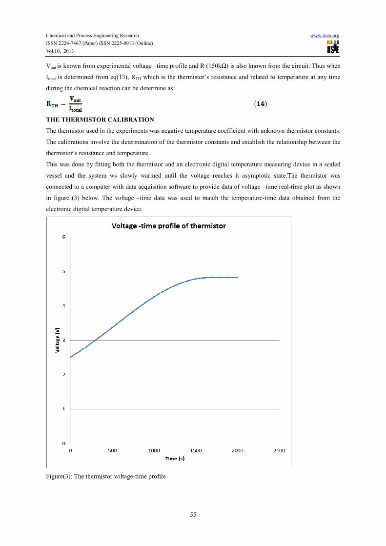
This was done by fitting both the thermistor and an electronic digital temperature measuring device in a sealed

vessel and the system ws slowly warmed until the voltage reaches it asymptotic state.The thermistor was

connected to a computer with data acquisition software to provide data of voltage –time real-time plot as shown

in figure (3) below. The voltage –time data was used to match the temperature-time data obtained from the

electronic digital temperature device.

Figure(3): The thermistor voltage-time profile



Vol.10, 2013

56

Figure(4): The thermistor temperature-time profile

RELATIONSHIP BETWEEN THERMISTOR RESISTANCE AND

TEMPERATURE

Thermistor resistance (RTH) and Temperature (T) in Kelvin was modeled using the empirical equation given

developed by Considine (1957)

or



Vol.10, 2013

57

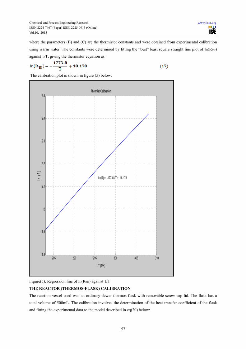
where the parameters (B) and (C) are the thermistor constants and were obtained from experimental calibration

using warm water. The constants were determined by fitting the “best” least square straight line plot of ln(RTH)

against 1/T, giving the thermistor equation as:

The calibration plot is shown in figure (5) below:

285 290 295 300 305 31011.8

11.9

12

12.1

12.2

12.3

12.4

12.5

1/T (1/K)

Ln

(R

)

Thermist Calibration

Ln(R) = -1773.8/T + 18.178

Figure(5): Regression line of ln(RTH) against 1/T

THE REACTOR (THERMOS-FLASK) CALIBRATION

The reaction vessel used was an ordinary dewer thermos-flask with removable screw cap lid. The flask has a

total volume of 500mL. The calibration involves the determination of the heat transfer coefficient of the flask

and fitting the experimental data to the model described in eq(20) below:



Vol.10, 2013

58

In this experiment 400.00g of distilled water at 361K (TO) was injected into the reaction vessel and left the

system temperature to fall over a period of time until the temperature-time profile reaches its asymptotic state or

the steady-state temperature (TS). The figure (6) below shows the temperature-time profile of the cooling

process.

0 10 20 30 40 50 60 70 80290

300

310

320

330

340

350

360

370

Time (hrs)

Tem

pera

ture

(K

)

Temperature -time Curve of cooling water in reaction vessel

T = T(s) + [(T(o) -T(s)]exp[-UA/mCp .t]

Fig (6) : Thermos-flask cooling curve at T(0) =361K

From eq(20) the values of To and Ts were obtained from fig(6.6). Rearrangement of eq(18) gives;

Since T and t values are known least square regression analysis was performed and a straight plot of ln(β)

against time is shown in figure (7) below:



Vol.10, 2013

59

0 500 1000 1500 2000 2500 3000 3500 4000-5

-4.5

-4

-3.5

-3

-2.5

-2

-1.5

-1

-0.5

0

Time(s)

Ln

(Y)

A Graph of Ln(Y) against Time of Cooling Water

Initial Temperature of water =361K

Ln (Y) = -0.0013.t

Mass of water = 400.0g

Fig (7) :Regression line of heat transfer coefficient of reactor

The slope of the straight line of fig(7) is given by 0.0013s-1

(min-1

) which corresponds to the value of the heat

transfer coefficient of the flask.

EXPERIMENTAL PROCEDURES AND RESULTS

Analytical reagent grade acetic anhydride was used in all the experiments. In all experiments about 1.0 mol of

acetic anhydride was poured into the reaction vessel followed by 3.0mols of the methanol. These volumes were

used so that at least 60% of the length of the sensor (thermistor) would be submerged in the resulting mixture.

Reactants were brought to a steady-state temperature before starting the stirrer. In course of the reaction the

stirrer speed was set 1000/ min and the resulting voltage-time profiles were captured as described above and the

corresponding temperature-time curve was determined using the thermistor equation derive in equation (17)

above. Runs were carried out adiabatically at the following initial temperatures: 290K, 294K and 300K.



Vol.10, 2013

60

DETERMINATION OF UA/mCp FOR THE REACTION MIXTURE

For a given system (reaction vessel and content) one can write:

In this experiment different amount of water (mw) (200g, 300g and 400g) was injected into the reaction flask at

343.08K, 347.77K and 347.85K and allowed to cool until the temperature reaches a steady-state temperature

(TS). Figures (8a), (9a) and (10a) of the cooling processes are shown below. The cooling process thus follows

equation (18) above. A nonlinear least-square regression analysis was performed on all the three experimental

curves. Using eq(19), the value of UA/mCP for each cooling curve was obtained. Figures (8b),(9b) and (10b)

shows the regression lines.

Fig (8a): Thermos-flask cooling curve at T(0) =343.08K



Vol.10, 2013

61

Fig (8b): Regression line of heat transfer coefficient of reactor



Vol.10, 2013

62




Vol.10, 2013

63




Vol.10, 2013

64




Vol.10, 2013

65


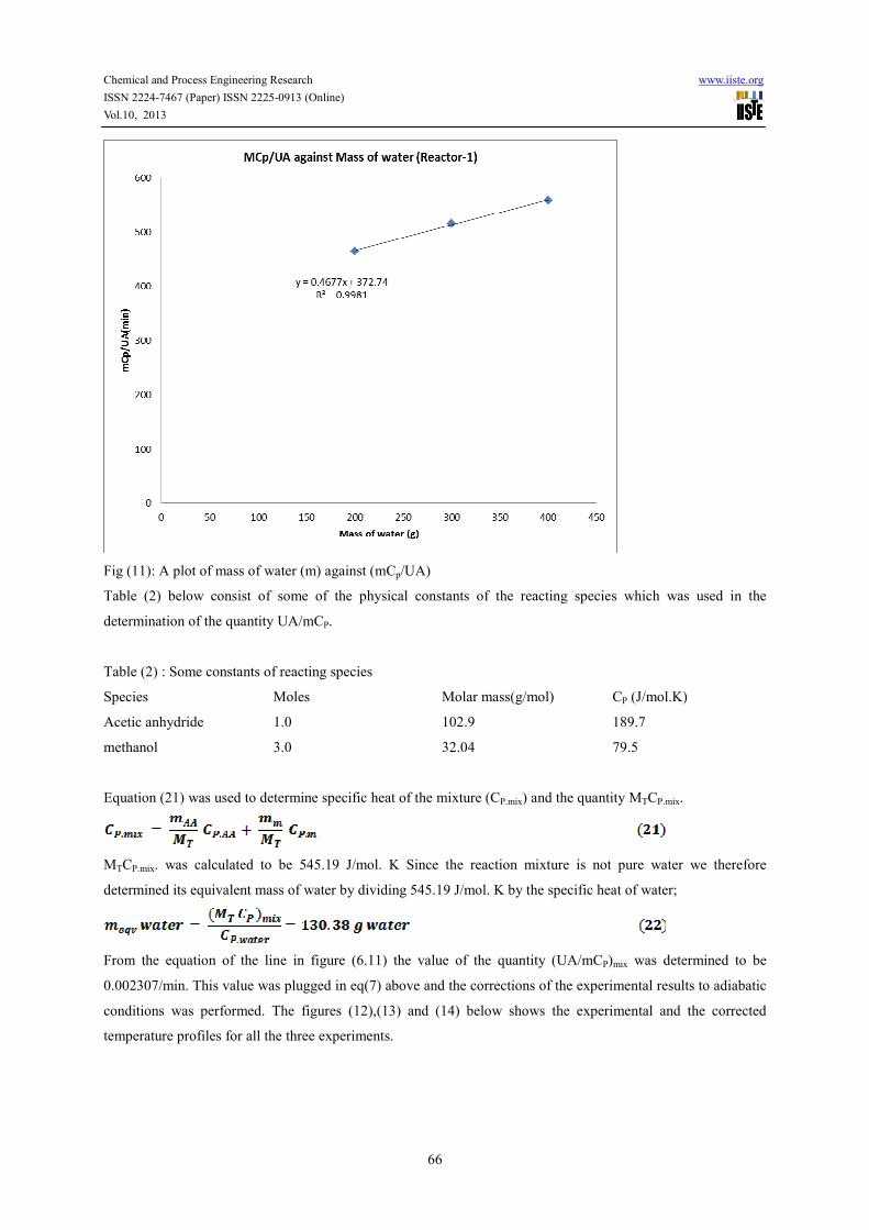
Table (1): Summary of characteristics of figures (6.8)-(6.10)

Mass of water(g) Initial Temperature(K) Final Temperature(K) UA/mCp (min-1

)

200 343.08 292.13 0.00215

300 347.77 293.00 0.00189

400 347.84 293.38 0.00178

From table (1) a plot of mass of water (m) against (mCp/UA) is shown in figure(11) below:



Vol.10, 2013

66

Fig (11): A plot of mass of water (m) against (mCp/UA)

Table (2) below consist of some of the physical constants of the reacting species which was used in the

determination of the quantity UA/mCP.

Table (2) : Some constants of reacting species

Species Moles Molar mass(g/mol) CP (J/mol.K)

Acetic anhydride 1.0 102.9 189.7

methanol 3.0 32.04 79.5

Equation (21) was used to determine specific heat of the mixture (CP.mix) and the quantity MTCP.mix.

MTCP.mix. was calculated to be 545.19 J/mol. K Since the reaction mixture is not pure water we therefore

determined its equivalent mass of water by dividing 545.19 J/mol. K by the specific heat of water;

From the equation of the line in figure (6.11) the value of the quantity (UA/mCP)mix was determined to be

0.002307/min. This value was plugged in eq(7) above and the corrections of the experimental results to adiabatic

conditions was performed. The figures (12),(13) and (14) below shows the experimental and the corrected

temperature profiles for all the three experiments.



Vol.10, 2013

67

0 50 100 150 200 250290

300

310

320

330

340

350

Time(min)

Te

mp

era

ture

(K

)

Experimental curve

Adiabatic curve

Fig(12): Experimental and Adiabatic curves of experiment-1



Vol.10, 2013

68

0 20 40 60 80 100 120 140 160 180 200290

300

310

320

330

340

350

Time (min)

Te

mp

era

ture

(K)

Experimental curve

Adiabatic curve




Vol.10, 2013

69

0 50 100 150 200 250 300290

300

310

320

330

340

350

Time(min)

Te

mp

era

ture

(K

)

Experimental curve

Adiabatic curve


Table (3) : Summary of the characteristics of the above temperature-time plot

Experiment T(0)(K) Tmax(adiabatic)(K) ∆Texp(adiabatic)(K)

1 290.01 345.80 55.69

2 294.00 345.60 51.9

3 299.20 345.30 46.13

From eq(9) the variation of acetic anhydride concentration with temperature/time was deduces as:

The constant (β) in eq(23) was calculated using the initial concentration of the acetic anhydride 4.364 mol/L and

the adiabatic theoretical temperature change (∆T)adiabatic. The figures (15),(16) and (17) show how acetic

anhydride concentration varies with time for the three experiments.



Vol.10, 2013

70

0 50 100 150 200 2502.6

2.8

3

3.2

3.4

3.6

3.8

4

4.2

4.4

4.6

Time(min)

Co

nc

en

tra

tio

n (

mo

l/L

)

Fig (15): Concentration-time plot of acetic anhydride-Exp(1)



Vol.10, 2013

71

0 20 40 60 80 100 120 140 160 180 2002.8

3

3.2

3.4

3.6

3.8

4

4.2

4.4

Time (min)

Co

nc

en

tra

tio

n(m

ol/

L)

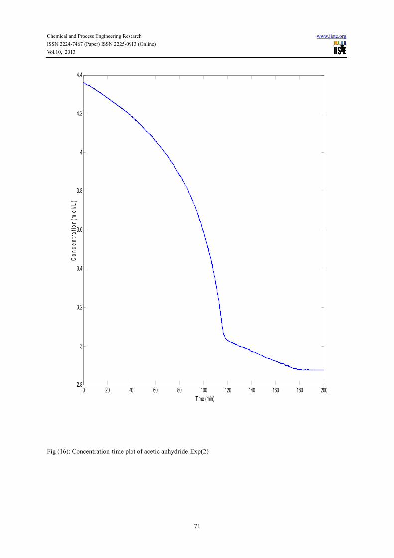
Fig (16): Concentration-time plot of acetic anhydride-Exp(2)



Vol.10, 2013

72

0 50 100 150 200 2503

3.5

4

4.5

Time (min)

Co

nc

en

tra

tio

n(m

ol/

L)

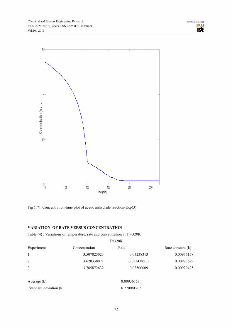
Fig (17): Concentration-time plot of acetic anhydride reaction-Exp(3)

VARIATION OF RATE VERSUS CONCENTRATION

Table (4) : Variations of temperature, rate and concentration at T =320K

T=320K

Experiment Concentration Rate Rate constant (k)

1 3.507025023 0.03238313 0.00936158

2 3.620338071 0.033438511 0.00923629

3 3.765872632 0.03500009 0.00929425

Average (k) 0.00936158

Standard deviation (k) 6.27008E-05



Vol.10, 2013

73

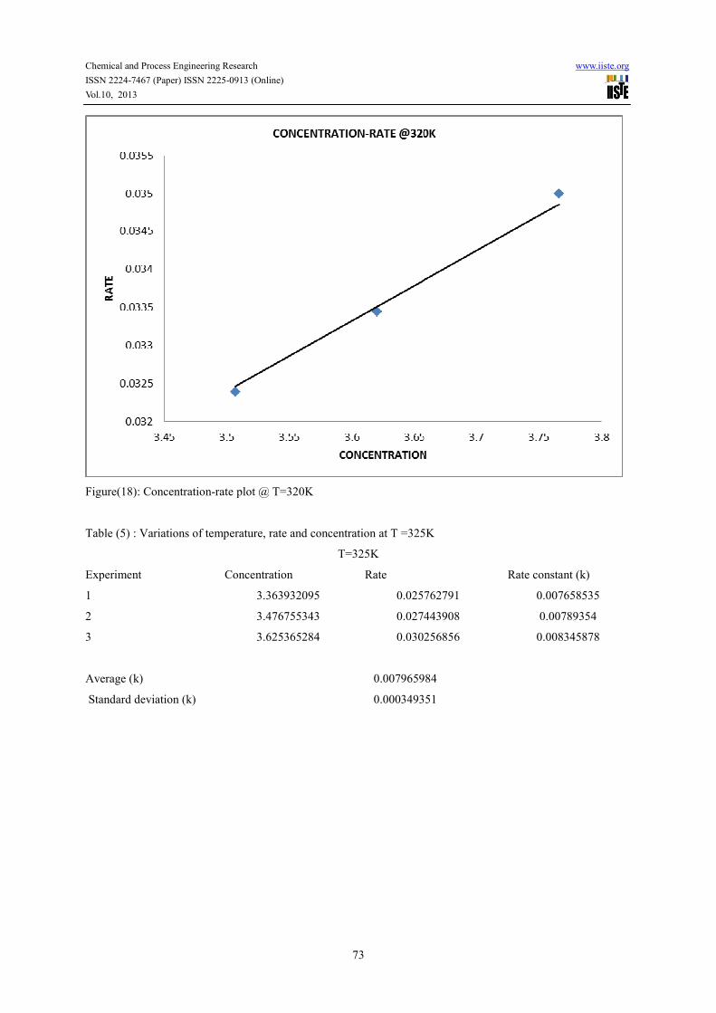
Figure(18): Concentration-rate plot @ T=320K


T=325K


1 3.363932095 0.025762791 0.007658535

2 3.476755343 0.027443908 0.00789354

3 3.625365284 0.030256856 0.008345878

Average (k) 0.007965984

Standard deviation (k) 0.000349351



Vol.10, 2013

74

Figure(19): Concentration-rate plot @ 325K


T=335K


1 3.077605537 0.041685326 0.013544727

2 3.186062023 0.04299617 0.013495082

3 3.339671258 0.045253824 0.013550382

Average (k) 0.013530064

Standard deviation (k) 3.04267E-05



Vol.10, 2013

75

Figure(20): Concentration-rate plot @ 335K

KINETICS AND THERMODYNAMIC ANALYSIS OF THE

EXPERIMENTS

The rate information obtained from the concentration-time plot enabled one to calculated specific rate constant

k(T) of the processes at any time (t) and temperature (T).

Arrhenius plots was thus generated from which kinetic parameters of the runs was extracted. The figures (21),

(22) and (23) below show the Arrhenius plots for all the three experiments.



Vol.10, 2013

76

Figure (21): Arrhenius plot of experiment-1



Vol.10, 2013

77




Vol.10, 2013

78


The values obtained for the specific rate constants as a function of temperature are given in equations (24),(25)

and (26) below:



Vol.10, 2013

79

The thermodynamic information extracted from the experiments was the heat of the reaction (∆Hrxn). This was

assumed to be independent of temperature and was determined by using eq(10). Table(7) below shows ∆Hr

values of the various experiments.

Table (7): Thermodynamic information of the experiments

Experiment 1 2 3

∆Hrxn(kJ/mol) 61.59 61.58 61.58

MODELING APPROACH

The experimental work discussed has shown that the reactions between the acetic anhydride and methanol

occurring in adiabatic batch reactor (thermos-flask) exhibit a first order reaction kinetics with respect to the

acetic anhydride. This is discussed in the section 6.8 above. The kinetic parameters of the reactions are discussed

in section 6.9 above. Thus for a first order adiabatic batch process, one can write design equation, rate law

expression and stiochiometry equations describing the process are as follow:

a) Design Equation:

b) Rate law:

c) Stiochiometry:

It assumed that since there is negligible or no change in density during the course of the reaction, the total

volume (V) is considered to be constant. Combining equations (27) –(29), a differential equation describing the

rate of change of conversion (X) with respect to time can be written as:

The kinetic parameters, pre-exponential constant (A) and the activation energy (EA) has been determined

experimentally in all the three reactions as discussed in section 6.9 above. The adiabat of the processes can be

written as:

Differentiating equation (32) with respect to time and plugging in equation (30) gives equation (33):



Vol.10, 2013

80

For a given process, given To, ∆Ta, A and Ea as initial starting points, simultaneous solution of equations (33)

and (34) with the help of Matlab (R2010a) program was used in the simulations process.

MODEL VALIDATION

The formulated models were validated by direct analysis and comparison of the model –predicted temperature

(T) and the values obtained from experimental measurements for equality. Analysis and the comparison between

the model predicted temperature values and the experimentally measured temperature values show some amount

of deviation of the model-predicted temperature values from the experimentally measured values. The deviation

in model equations results may be due to non-incorporation of some practical conditions in the model equation

and solution strategy. Also assumptions made in the model equation’s development may be responsible in the

deviation of the model results. This can be improved by refining the model equation, and introduction of

correction factor to the bring model- predicted temperature values to those of the experimental values.Percentage

deviation (% Dmodel) of model-predicted temperature from experimentally measured values is given by equation

(35) below:

where the correction factor (β) = -(Dmodel) (36)

and (M)-model-predicted temperature, and (E)-experimentally measured temperature.

The model is also validated by considering the correlation coefficients (R2 ) of the model-predicted temperature

and the experimentally measured temperature.



Vol.10, 2013

81

RESULTS

Figure (24a): Comparison of the model- predicted and experimentally measured temperature for experiment (1)



Vol.10, 2013

82

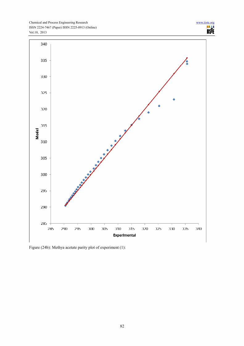
Figure (24b): Methya acetate parity plot of experiment (1):



Vol.10, 2013

83

Figure (24c): Variation of model-predicted temperature with its associated deviation from experimental results-

Experiment (1)



Vol.10, 2013

84

Figure (24d): Variation of model-predicted temperature with its associated correction factor-Experiment (1)



Vol.10, 2013

85

Figure (25a): Comparison of the model- predicted and experimentally measured temperature against time for

experiment (2)



Vol.10, 2013

86

Figure (25b) show the parity plot of model-predicted and experimentally measured temperature of experiment

(2):



Vol.10, 2013

87


Experiment (2)



Vol.10, 2013

88




Vol.10, 2013

89

Figure (26a): Comparison of the model- predicted and experimentally measured temperature against time for

experiment (3)



Vol.10, 2013

90

Figure (26b) show the parity plot of model-predicted and experimentally measured temperature of experiment

(3)



Vol.10, 2013

91


Experiment (3)



Vol.10, 2013

92


DISCUSSIONS

By direct comparison of model-predicted temperature profiles and experimentally measure temperature profiles

it is seen if figures 24a, 25a and 26a the model proposed agree quite well in predicting the experimentally

measure temperatures. The parity plots shown in figures 24b, 25b and 26c are also used as a means of validation

of the proposed model. It is seen from the plots that there is good agreement between model-predicted

temperatures and experimentally measured temperatures. An ideal comparison testing validity of the model is



Vol.10, 2013

93

achieved by considering the r-squared values (coefficient of determination). Comparing the data from both the

model and the experiment it was noticed that the r-squared values were 0.980,0.991 and 0.994 respectively for

experiments 1, 2 and 3. This suggest proximate agreement between model-predicted temperatures and that of the

experimentally measure temperatures. The maximum percentage deviations of the model-predicted temperatures,

from the corresponding experimental values are 3.18%, 1.83% and 3.86% for experiments 1, 2 and 3. The

deviations are depicted graphically in figures 24c, 25c and 26c. The deviation values are quite within the

acceptable deviation range of experimental results and give an indication of the reliability the usefulness of the

proposed model. The correction factors which were the negative form of the deviations are shown in figures 24d,

25d and 26d. The correction factors take care of the effects of all the issues that were not considered during the

experiments and the assumptions which were not catered for during the model formulation. The model as it

stands can be used to predict liquid- phase temperature of the esterification process of acetic anhydride and

methanol. The predicted temperatures can then be used to predict the liquid phase composition with the help of

equation (9) above during reactive distillation process until the reaction reaches the maximum steady boiling

temperature of 335K. At this near boiling temperature one expects the vapor-phase of the system to consist of

some reactants and products species and by thermodynamic considerations the vapor-phase compositions can be

predicted. This then constitute a step toward the preliminary design of reactive distillation system of the

esterification process of acetic anhydride with methanol.

CONCLUSIONS

The mathematical models developed have shown satisfactory results in simulating the liquid-phase temperatures

of the esterification of acetic anhydride with methanol. The results were found in good agreement with

experimental results. The maximum deviation of the model-predicted temperatures was found to be not more

than 4% in all cases which is quiet within acceptable range of experimental results. Nonetheless, further work

should incorporate more process parameters into the model with the aim of reducing the deviations of the model-

predicted temperature values from those of the experimentally measured observed values. The findings from the

simulation results can be used to develop the technology (reactive distillation) to convert acetic anhydride-

methanol system to methyl acetate and acetic acid.

LIST OF SYMBOLS

∆Hrxn-heat of reaction (KJ/mol)

H-Enthalpy

Ho- Initial Enthalpy

∆T (ad) –adiabatic temperature change (K)

∆ε –extent of reaction

A –preexponential factor

B,C – thermistor constants

CA-concentration of A (mol/L)

CP –specific heat capacity

CP,AA –specific heat capacity of acetic anhydride

CP,m –specific heat capacity of methanol

CP,mix-constant heat capacity of reaction mixture (kJ/mol.K)

CP,W –specific heat capacity of water

Ea – activation energy

Itotal – total current of the circuit

Ko

eqm –Equilibrium constant

m –mass

MAA –Mass of acetic anhydride

Mm –Mass of methanol

Meqv –Equivalent amount of water

MT-mass of reaction mixture(Kg)

NA –mole of A (mol)

Q-heat produced by stirrer

R – molar gas constant

R2 – known resistance in the circuit

-rA –rate of reaction of (A)

RTH – Thermistor resistance

t – time

Tamb –ambient temperature



Vol.10, 2013

94

Tmax –maximum temperature (K)

To –initial temperature

T-reactor temperature (K)

TS – steady state temperature (K)

U –heat transfer coefficient (J/m2 s.K)

v – total voltage of the circuit

V-Volume of vessel

Vout – voltage measured by thermistor

VTH – voltage across thermistor resistance

X- conversion

β- constant

REFERENCES

Agreda, V. H., Partin, L. R., Heise, L. R., (1990), “High-Purity Methyl Acetate via Reactive Distillation”, Chem.

Eng. Prog. Vol 86 No.2, 40-46.

Bock, H., Jimoh, M., Wozny, G. (1997), “Analysis of Reactive Distillation using the Esterification of Acetic

Acid as an example”, Chem. Eng. Technol. 20 182 -191.

Kenig, E. Y., Bäder, H., Górak, A., Beβling, B., Adrian, T., Schoenmakers, H., (2001),“Investigation of Ethyl

Acetate Reactive Distillation Process”, Chem. Eng. Sci.”,6185 -6193.

Keys, D. B., (1932), “ Esterification Processes and Equipment”, Ind. Eng. Chem., Vol. 24, 1096 -1103.

Kreul, U. L., Gorak, A., Dittrich, C., (1998), “Catalytic Distillation: Advanced Simulation and Experimental

Validation”, Comp. Chem. Eng. Vol 22, 371 -373

Mohl, K, D., Kienle, A., Gilles, E. D., Rapmund, P., Sundmacher, K., Hoffmann, U. (1997), “Nonlinear

Dynamics of Reactive Distillation Processes for the Production of Fuel Ether”, Comp. Chem. Eng. Vol 21, S983-

S994.

Popken, T., Steinigeweg, S., Gmehling, J., (2001), “Synthesis and Hydrolysis of Methyl Acetate Reactive

Distillation using Structured Catalytic Packing: Experiments ans Simulation”, Ind. Eng. Chem. Res., Vol. 40,

1566 -1574.

Teo, H. T. R., Saha, B., (2004),” Heterogeneous Catalysed Esterification of Acetic Acid with Isoamyl Alcohol:

Kinetic Studied”, J. Catal. 228 174 -182.

Date post:	11-May-2015
Category:	Technology
Upload:	alexander-decker
View:	114 times
Download:	2 times

Modeling and simulation of temperature profiles in a reactive

Technology