+ All Categories
Home > Documents > Modeling and Simulation of the ECOSat-III Attitude ...€¦ · Modeling and Simulation of the...

Modeling and Simulation of the ECOSat-III Attitude ...€¦ · Modeling and Simulation of the...

Date post: 30-Apr-2020
Category:
Upload: others
View: 3 times
Download: 0 times
Share this document with a friend
130
Modeling and Simulation of the ECOSat-III Attitude Determination and Control System Duarte Otero de Morais Alves Rondão Thesis to obtain the Master of Science Degree in Aerospace Engineering Supervisor: Prof. Afzal Suleman Examination Committee Chairperson: Prof. João Manuel Lage de Miranda Lemos Supervisor: Prof. Afzal Suleman Member of the Committee: Prof. Paulo Jorge Coelho Ramalho Oliveira April 2016
Transcript

Modeling and Simulation of the ECOSat-III AttitudeDetermination and Control System

Duarte Otero de Morais Alves Rondão

Thesis to obtain the Master of Science Degree in

Aerospace Engineering

Supervisor: Prof. Afzal Suleman

Examination Committee

Chairperson: Prof. João Manuel Lage de Miranda LemosSupervisor: Prof. Afzal SulemanMember of the Committee: Prof. Paulo Jorge Coelho Ramalho Oliveira

April 2016

ii

Acknowledgments

I would like to thank my supervisor Dr. Afzal Suleman for the research opportunity on such an exciting field and

for his assistance during the research and writing of this thesis. Additionally, I want to thank the ECOSat team of

the Center for Aerospace Research at the University of Victoria for providing a hands-on experience in satellite

mission design in a whole new continent. I wish the team the best of luck for the development of the mission in

the future.

I wish to express my gratitude to Prof. Fernando Lau for taking the time to carefully review this dissertation and

for his helpful insight on the matter.

I would also like to thank the experts consulted during this research project: Dr. Daniel Choukroun of the Space

Engineering department at the Delft University of Technology, and Mr. Alireza Khosravian of the College of

Engineering & Computer Science at the Australian National University. Without their valuable participation and

input, this research thesis could not have been successfully conducted.

During my course as an aerospace engineering student in Lisbon, Delft and Victoria, I had the pleasure of meeting

different people from around the world who are, unfortunately, far too many to enumerate but who have made this

journey far more pleasant than what it already was. Thank you.

I would like to conclude by thanking my family for their everyday support, for pushing and encouraging me to take

a chance and to follow my ambitions.

Lisbon, Portugal

02/04/2016Duarte Rondão

iii

iv

Resumo

A determinação e controlo de atitude em CubeSats é desafiante devido a restrições de volume e à falta de

pequenos sensores de atitude. Adicionalmente, os sistemas de controlo de atitude nestes satélites utilizam tipi-

camente “magnetorquers” como actuadores, que têm eficácia reduzida a inclinações orbitais menores e sofrem

de uma precisão inferior comparativamente a rodas de reacção. Deste modo, a maioria dos designs de controlo

para CubeSats contêm erros de atitude consideráveis. Nesta tese é proposto um sistema de determinação de

atitude e controlo (ADCS) que utiliza sensores e actuadores de baixo custo e permite obter uma precisão de di-

recionamento superior a 4.78 deg. Realiza-se o desenvolvimento e comparação de quatro diferentes algoritmos

de estimação que utilizam medições provenientes de um sensor solar, magnetómetro, e giroscópio de sistemas

micro-electromecânicos (MEMS). O “multiplicative extended Kalman filter” (MEKF) é implementado como base

comparativa para os outros três algoritmos: o “unscented quaternion Kalman filter” (UQKF), o “two-step optimal

estimator” (2STEP), e o “constant gain geometric attitude observer” (GEOB). Para o controlo de atitude, uma ver-

são melhorada da lei “B-dot” que utiliza “magnetorquers” é implementada para o “detumbling”. Um controlador

em “sliding mode” é empregado para a fase nominal de “Earth-tracking” utilizando um sistema especial de rodas

de reacção (RWS). Um sistema de “dumping” de momento utilizando os “torquers” é implementado para garantir

que o RWS evita a saturação. São realizadas simulações no âmbito do satélite ECOSat-III. O ADCS proposto

garante um erro de direcionamento abaixo dos 2 deg e um “detumbling” em 3.5 órbitas.

Palavras-chave - Determinação de atitude, controlo de atitude, CubeSat, estimação não-linear, controlo não-

linear, filtro de Kalman

v

vi

Abstract

Attitude determination and pointing control in cube satellites is challenging mainly due to volumetric constraints

and lack of small attitude sensors. In addition, the attitude control systems in CubeSats typically employ magne-

torquers as the main actuators, which become less effective at lower orbital inclinations and suffer from reduced

pointing accuracy when compared to reaction wheels. As a result, most CubeSat control designs are character-

ized by considerable pointing errors. In this thesis, an attitude determination and control system (ADCS) using

low-cost sensors and actuators that allows for a pointing accuracy better than 4.78 deg is proposed. The de-

velopment and comparison of four attitude estimation algorithms is performed using sun sensor, magnetometer,

and micro-electromechanical systems (MEMS) gyro measurements. The multiplicative extended Kalman filter

(MEKF) is implemented as a benchmark for the other three algorithms: the unscented quaternion Kalman filter

(UQKF), the two-step optimal estimator (2STEP), and the constant gain geometric attitude observer (GEOB).

For attitude control, an enhanced version of the B-dot control law using magnetorquers is implemented for the

detumbling stage. A three-axis sliding mode controller is employed for the nominal, Earth-tracking phase, using a

specially designed reaction wheel system (RWS). A momentum dumping system using the magnetic torquers is

also devised to ensure that the RWS does not reach saturation. Simulations are performed in an environment for

the ECOSat-III CubeSat. The proposed ADCS yields a pointing error lower than 2 deg and detumbles the satellite

in 3.5 orbits.

Keywords - Attitude determination, attitude control, CubeSat, nonlinear estimation, nonlinear control, Kalman

filtering

vii

viii

Contents

Acknowledgments . . . . . . . . . . . . . . . . . . . . . . . . . . . . . . . . . . . . . . . . . . . . . . iii

Resumo . . . . . . . . . . . . . . . . . . . . . . . . . . . . . . . . . . . . . . . . . . . . . . . . . . . v

Abstract . . . . . . . . . . . . . . . . . . . . . . . . . . . . . . . . . . . . . . . . . . . . . . . . . . . vii

List of Tables xiii

List of Figures xv

List of Algorithms xvii

List of Theorems and Definitions xix

List of Acronyms and Abbreviations xxii

List of Symbols xxviii

1 Introduction 1

1.1 Context . . . . . . . . . . . . . . . . . . . . . . . . . . . . . . . . . . . . . . . . . . . . . . . . . 1

1.2 The Enhanced Communications Satellite Project . . . . . . . . . . . . . . . . . . . . . . . . . . . 2

1.2.1 Mission Objectives . . . . . . . . . . . . . . . . . . . . . . . . . . . . . . . . . . . . . . . 2

1.2.2 Pointing Requirements . . . . . . . . . . . . . . . . . . . . . . . . . . . . . . . . . . . . . 3

1.2.3 ADCS Operation Modes . . . . . . . . . . . . . . . . . . . . . . . . . . . . . . . . . . . . 4

1.3 Literature Study . . . . . . . . . . . . . . . . . . . . . . . . . . . . . . . . . . . . . . . . . . . . 5

1.4 Motivation and Goals . . . . . . . . . . . . . . . . . . . . . . . . . . . . . . . . . . . . . . . . . 6

1.5 Overview of the Dissertation . . . . . . . . . . . . . . . . . . . . . . . . . . . . . . . . . . . . . . 7

2 Theoretical Background 8

2.1 Parameterizations of the Attitude . . . . . . . . . . . . . . . . . . . . . . . . . . . . . . . . . . . 8

2.1.1 Direction Cosine Matrix . . . . . . . . . . . . . . . . . . . . . . . . . . . . . . . . . . . . 8

2.1.2 Euler Axis/Angle . . . . . . . . . . . . . . . . . . . . . . . . . . . . . . . . . . . . . . . . 9

2.1.3 Quaternion . . . . . . . . . . . . . . . . . . . . . . . . . . . . . . . . . . . . . . . . . . . 9

2.1.4 Modified Rodrigues Parameters . . . . . . . . . . . . . . . . . . . . . . . . . . . . . . . . 11

2.2 Frames of Reference . . . . . . . . . . . . . . . . . . . . . . . . . . . . . . . . . . . . . . . . . . 11

2.2.1 Spacecraft Body Frame . . . . . . . . . . . . . . . . . . . . . . . . . . . . . . . . . . . . 12

2.2.2 Earth-Centered Inertial Frame . . . . . . . . . . . . . . . . . . . . . . . . . . . . . . . . . 12

2.2.3 Earth-Centered/Earth-Fixed Frame . . . . . . . . . . . . . . . . . . . . . . . . . . . . . . 12

2.2.4 Local-Vertical/Local-Horizontal Frame . . . . . . . . . . . . . . . . . . . . . . . . . . . . . 13

2.3 Stability Theory for Nonlinear Systems . . . . . . . . . . . . . . . . . . . . . . . . . . . . . . . . 14

2.3.1 Stability Definitions . . . . . . . . . . . . . . . . . . . . . . . . . . . . . . . . . . . . . . . 14

2.3.2 Stability of the Origin . . . . . . . . . . . . . . . . . . . . . . . . . . . . . . . . . . . . . . 15

2.3.3 Stability Theorems . . . . . . . . . . . . . . . . . . . . . . . . . . . . . . . . . . . . . . . 15

2.3.4 Global Stabilization of Spacecraft Rotational Motion . . . . . . . . . . . . . . . . . . . . . 16

ix

3 Spacecraft Mechanics 17

3.1 Orbital Mechanics . . . . . . . . . . . . . . . . . . . . . . . . . . . . . . . . . . . . . . . . . . . 17

3.2 Attitude Kinematics . . . . . . . . . . . . . . . . . . . . . . . . . . . . . . . . . . . . . . . . . . 19

3.3 Attitude Dynamics . . . . . . . . . . . . . . . . . . . . . . . . . . . . . . . . . . . . . . . . . . . 20

3.4 Spacecraft Perturbations . . . . . . . . . . . . . . . . . . . . . . . . . . . . . . . . . . . . . . . . 22

3.4.1 Perturbative Forces . . . . . . . . . . . . . . . . . . . . . . . . . . . . . . . . . . . . . . 22

3.4.2 Perturbative Torques . . . . . . . . . . . . . . . . . . . . . . . . . . . . . . . . . . . . . . 25

4 Sensor and Actuator Hardware 28

4.1 Sensors . . . . . . . . . . . . . . . . . . . . . . . . . . . . . . . . . . . . . . . . . . . . . . . . 28

4.1.1 Inertial Sensors . . . . . . . . . . . . . . . . . . . . . . . . . . . . . . . . . . . . . . . . 29

4.1.2 Reference Sensors . . . . . . . . . . . . . . . . . . . . . . . . . . . . . . . . . . . . . . . 29

4.2 Actuators . . . . . . . . . . . . . . . . . . . . . . . . . . . . . . . . . . . . . . . . . . . . . . . . 30

4.2.1 Momentum and Reaction Wheels . . . . . . . . . . . . . . . . . . . . . . . . . . . . . . . 31

4.2.2 Magnetic Torquers . . . . . . . . . . . . . . . . . . . . . . . . . . . . . . . . . . . . . . . 31

4.2.3 Other Actuators . . . . . . . . . . . . . . . . . . . . . . . . . . . . . . . . . . . . . . . . 32

4.3 Hardware Selection . . . . . . . . . . . . . . . . . . . . . . . . . . . . . . . . . . . . . . . . . . 32

5 Recursive Attitude Determination 36

5.1 Kalman Filtering . . . . . . . . . . . . . . . . . . . . . . . . . . . . . . . . . . . . . . . . . . . . 36

5.2 The Extended Kalman Filter . . . . . . . . . . . . . . . . . . . . . . . . . . . . . . . . . . . . . . 40

5.2.1 The Additive EKF . . . . . . . . . . . . . . . . . . . . . . . . . . . . . . . . . . . . . . . . 42

5.2.2 The Multiplicative EKF . . . . . . . . . . . . . . . . . . . . . . . . . . . . . . . . . . . . . 43

5.3 Unscented Filtering . . . . . . . . . . . . . . . . . . . . . . . . . . . . . . . . . . . . . . . . . . 48

5.3.1 The Unscented Quaternion Kalman Filter . . . . . . . . . . . . . . . . . . . . . . . . . . . 49

5.4 The Two-Step Optimal Estimator . . . . . . . . . . . . . . . . . . . . . . . . . . . . . . . . . . . 52

5.5 Geometric Observers . . . . . . . . . . . . . . . . . . . . . . . . . . . . . . . . . . . . . . . . . 56

5.5.1 Constant Gain Geometric Attitude Observer . . . . . . . . . . . . . . . . . . . . . . . . . 57

6 Attitude Control 59

6.1 Nominal Mode . . . . . . . . . . . . . . . . . . . . . . . . . . . . . . . . . . . . . . . . . . . . . 59

6.1.1 Optimal Sliding-Mode Controller . . . . . . . . . . . . . . . . . . . . . . . . . . . . . . . . 60

6.2 Momentum Dumping . . . . . . . . . . . . . . . . . . . . . . . . . . . . . . . . . . . . . . . . . . 62

6.3 Detumbling Mode . . . . . . . . . . . . . . . . . . . . . . . . . . . . . . . . . . . . . . . . . . . 63

7 Simulation Environment 65

7.1 Spacecraft Mechanics Simulator . . . . . . . . . . . . . . . . . . . . . . . . . . . . . . . . . . . 65

7.1.1 Eclipse Calculation . . . . . . . . . . . . . . . . . . . . . . . . . . . . . . . . . . . . . . . 65

7.2 Hardware Models . . . . . . . . . . . . . . . . . . . . . . . . . . . . . . . . . . . . . . . . . . . 66

7.2.1 Gyroscope Model . . . . . . . . . . . . . . . . . . . . . . . . . . . . . . . . . . . . . . . 66

7.2.2 Magnetometer Model . . . . . . . . . . . . . . . . . . . . . . . . . . . . . . . . . . . . . 67

7.2.3 Sun Sensor Model . . . . . . . . . . . . . . . . . . . . . . . . . . . . . . . . . . . . . . . 68

7.2.4 Magnetorquer System Model . . . . . . . . . . . . . . . . . . . . . . . . . . . . . . . . . 68

7.2.5 Reaction Wheel System Model . . . . . . . . . . . . . . . . . . . . . . . . . . . . . . . . 69

7.3 Attitude Determination and Control System . . . . . . . . . . . . . . . . . . . . . . . . . . . . . . 70

x

8 Testing 71

8.1 Results . . . . . . . . . . . . . . . . . . . . . . . . . . . . . . . . . . . . . . . . . . . . . . . . . 71

8.2 Discussion . . . . . . . . . . . . . . . . . . . . . . . . . . . . . . . . . . . . . . . . . . . . . . . 74

9 Closure 79

9.1 Conclusions . . . . . . . . . . . . . . . . . . . . . . . . . . . . . . . . . . . . . . . . . . . . . . 79

9.2 Recommendations . . . . . . . . . . . . . . . . . . . . . . . . . . . . . . . . . . . . . . . . . . . 80

A Review of Vector and Tensor Algebra 81

A.1 Vector and Tensor Notation . . . . . . . . . . . . . . . . . . . . . . . . . . . . . . . . . . . . . . 81

A.2 Matrix Representation of Vectors and Tensors . . . . . . . . . . . . . . . . . . . . . . . . . . . . 83

A.3 Change of Basis . . . . . . . . . . . . . . . . . . . . . . . . . . . . . . . . . . . . . . . . . . . . 83

A.4 Time Variation of Vectors . . . . . . . . . . . . . . . . . . . . . . . . . . . . . . . . . . . . . . . 85

B Hardware Parameters 86

B.1 Sensor Trade-off . . . . . . . . . . . . . . . . . . . . . . . . . . . . . . . . . . . . . . . . . . . . 86

B.2 Sensor Error Parameters . . . . . . . . . . . . . . . . . . . . . . . . . . . . . . . . . . . . . . . 86

C Supplementary Algorithms 88

C.1 DCM to Quaternion Mapping . . . . . . . . . . . . . . . . . . . . . . . . . . . . . . . . . . . . . 88

C.2 Attitude Estimation Flowcharts . . . . . . . . . . . . . . . . . . . . . . . . . . . . . . . . . . . . 89

C.3 Eclipse Calculation . . . . . . . . . . . . . . . . . . . . . . . . . . . . . . . . . . . . . . . . . . . 94

Bibliography 95

xi

xii

List of Tables

4.1 Effect of payload pointing directions on ADCS design for 3-axis controlled spacecraft . . . . . . . . 33

4.2 Effect of control accuracy on sensor selection and ADCS design . . . . . . . . . . . . . . . . . . 33

4.3 CRS09-01 characteristics . . . . . . . . . . . . . . . . . . . . . . . . . . . . . . . . . . . . . . . 34

4.4 RM3100 characteristics . . . . . . . . . . . . . . . . . . . . . . . . . . . . . . . . . . . . . . . . 34

4.5 NanoSSOC-A60 characteristics . . . . . . . . . . . . . . . . . . . . . . . . . . . . . . . . . . . . 34

4.6 Magnetorquer characteristics for individual rods . . . . . . . . . . . . . . . . . . . . . . . . . . . 35

4.7 RWS characteristics for individual flywheel/motor . . . . . . . . . . . . . . . . . . . . . . . . . . . 35

8.1 General simulation parameters . . . . . . . . . . . . . . . . . . . . . . . . . . . . . . . . . . . . 71

8.2 Estimator parameters . . . . . . . . . . . . . . . . . . . . . . . . . . . . . . . . . . . . . . . . . 72

8.3 Estimator run time parameters per iteration . . . . . . . . . . . . . . . . . . . . . . . . . . . . . . 72

8.4 Control gains . . . . . . . . . . . . . . . . . . . . . . . . . . . . . . . . . . . . . . . . . . . . . . 72

B.1 Performance and price comparison of MEMS gyros . . . . . . . . . . . . . . . . . . . . . . . . . 86

B.2 Performance and price comparison of magnetometers . . . . . . . . . . . . . . . . . . . . . . . . 86

B.3 Performance and price comparison of Sun sensors . . . . . . . . . . . . . . . . . . . . . . . . . . 87

B.4 HG1700 gyro error parameters per sensor axis . . . . . . . . . . . . . . . . . . . . . . . . . . . . 87

B.5 MAGIC error parameters per sensor axis . . . . . . . . . . . . . . . . . . . . . . . . . . . . . . . 87

xiii

xiv

List of Figures

1.1 ECOSat-III spacecraft and payloads . . . . . . . . . . . . . . . . . . . . . . . . . . . . . . . . . . 2

1.2 Concept of pointing . . . . . . . . . . . . . . . . . . . . . . . . . . . . . . . . . . . . . . . . . . 4

2.1 Definition of various reference frames . . . . . . . . . . . . . . . . . . . . . . . . . . . . . . . . . 12

3.1 Geometry of a spacecraft in an elliptical orbit about the Earth . . . . . . . . . . . . . . . . . . . . 18

3.2 Classical orbital elements . . . . . . . . . . . . . . . . . . . . . . . . . . . . . . . . . . . . . . . 19

4.1 Selected sensors for ECOSat-III . . . . . . . . . . . . . . . . . . . . . . . . . . . . . . . . . . . . 33

4.2 Selected actuators for ECOSat-III . . . . . . . . . . . . . . . . . . . . . . . . . . . . . . . . . . . 34

5.1 Operation of the Kalman filter . . . . . . . . . . . . . . . . . . . . . . . . . . . . . . . . . . . . . 37

7.1 Top hierarchical level of the ECOSat-III Simulink R© simulation environment . . . . . . . . . . . . . 66

7.2 Matlab R© Simulink R© gyroscope model . . . . . . . . . . . . . . . . . . . . . . . . . . . . . . . . 67

7.3 Matlab R© Simulink R© magnetometer model . . . . . . . . . . . . . . . . . . . . . . . . . . . . . . 67

7.4 Matlab R© Simulink R© Sun sensor model . . . . . . . . . . . . . . . . . . . . . . . . . . . . . . . . 68

7.5 Matlab R© Simulink R© magnetorquer model . . . . . . . . . . . . . . . . . . . . . . . . . . . . . . 68

7.6 Matlab R© Simulink R© reaction wheel model . . . . . . . . . . . . . . . . . . . . . . . . . . . . . . 69

8.1 Performance of attitude estimators in Case 1 . . . . . . . . . . . . . . . . . . . . . . . . . . . . . 73

8.2 Performance of attitude estimators in Case 2 . . . . . . . . . . . . . . . . . . . . . . . . . . . . . 73

8.3 Performance indicators in Case 3 . . . . . . . . . . . . . . . . . . . . . . . . . . . . . . . . . . . 74

8.4 Performance indicators in Case 4 . . . . . . . . . . . . . . . . . . . . . . . . . . . . . . . . . . . 75

xv

xvi

List of Algorithms

C.1 Computation of the best mapping from the DCM to the quaternion in terms of numerical accuracy . 89

C.2 MEKF algorithm flowchart . . . . . . . . . . . . . . . . . . . . . . . . . . . . . . . . . . . . . . . 90

C.3 UQKF algorithm flowchart . . . . . . . . . . . . . . . . . . . . . . . . . . . . . . . . . . . . . . . 91

C.4 2STEP algorithm flowchart . . . . . . . . . . . . . . . . . . . . . . . . . . . . . . . . . . . . . . . 92

C.5 GEOB algorithm flowchart . . . . . . . . . . . . . . . . . . . . . . . . . . . . . . . . . . . . . . . 93

C.6 Computation of eclipse status using a ray-sphere intersection method . . . . . . . . . . . . . . . . 94

xvii

xviii

List of Theorems and Definitions

2.1 Definition (L-Stability) . . . . . . . . . . . . . . . . . . . . . . . . . . . . . . . . . . . . . . . . . 14

2.2 Definition (Instability) . . . . . . . . . . . . . . . . . . . . . . . . . . . . . . . . . . . . . . . . . . 14

2.3 Definition (Attractive Solution) . . . . . . . . . . . . . . . . . . . . . . . . . . . . . . . . . . . . . 14

2.4 Definition (Asymptotic Stability) . . . . . . . . . . . . . . . . . . . . . . . . . . . . . . . . . . . . 14

2.5 Definition (Exponential Stability) . . . . . . . . . . . . . . . . . . . . . . . . . . . . . . . . . . . . 14

2.6 Definition (Global Asymptotic Stability) . . . . . . . . . . . . . . . . . . . . . . . . . . . . . . . . 15

2.1 Theorem (L-Stability) . . . . . . . . . . . . . . . . . . . . . . . . . . . . . . . . . . . . . . . . . . 15

2.2 Theorem (Asymptotic Stability) . . . . . . . . . . . . . . . . . . . . . . . . . . . . . . . . . . . . 15

2.3 Theorem (Global Asymptotic Stability) . . . . . . . . . . . . . . . . . . . . . . . . . . . . . . . . 15

2.4 Theorem ((Global) Exponential Stability) . . . . . . . . . . . . . . . . . . . . . . . . . . . . . . . 15

2.5 Theorem (Instability) . . . . . . . . . . . . . . . . . . . . . . . . . . . . . . . . . . . . . . . . . . 16

xix

xx

List of Acronyms and Abbreviations

2STEP two-step optimal estimator

ADC analog-to-digital converter

ADCS attitude determination and control system

AEKF additive extended Kalman filter

ARW angle random walk

BLDC brushless direct current

CAN controller area network

CCD charge-coupled device

CINEMA CubeSat for Ions, Neutrals, Electrons and MAgnetic

fields

CMG control moment gyro

CMOS complementary metal-oxide-semiconductor

COTS commercial-off-the-shelf

CSDC Canadian Satellite Design Challenge

CSS coarse Sun sensor

DC direct current

DCM direction cosine matrix

DSS digital Sun sensor

ECEF Earth-Centered/Earth-Fixed

ECI Earth-Centered Inertial

EGM96 Earth Gravitational Model 1996

EKF extended Kalman filter

EMF electromotive force

FOV field-of-view

GEOB constant gain geometric attitude observer

GMST Greenwich Mean Sidereal Time

GPS Global Positioning System

GRP generalized Rodrigues parameter

IGRF-12 International Geomagnetic Reference Field

IMU inertial measurement unit

JPL Jet Propulsion Laboratory

KF Kalman filter

LEO low Earth orbit

LLMSE linear least mean squares estimator

LOS line-of-sight

LVLH Local-Vertical/Local-Horizontal

MAGIC MAGnetometer from Imperial College

MEKF multiplicative extended Kalman filter

MEMS micro-electromechanical systems

MRP modified Rodrigues parameter

MSE mean square error

xxi

NORAD North American Aerospace Defense Command

NRLMSISE-00 Naval Research Laboratory Mass Spectrometer

and Incoherent Scatter Radar Exosphere

OBDH on-board data handling

PD proportional-derivative

PDF probability density function

PID proportional–integral–derivative

QUEST QUaternion ESTimator

RAAN right ascension of the ascending node

RG rate gyroscope

RGB red, green and blue

RIG rate-integrating gyroscope

RL resistor-inductor

RRW rate random walk

RV random variable

RWS reaction wheel system

S/C spacecraft

SMC sliding-mode control

SPARS Space Precision Attitude Reference System

SRP solar radiation pressure

SS Sun sensor

TAM three-axis magnetometer

UF unscented filter

UQKF unscented quaternion Kalman filter

USD United States dollars

USQUE unscented quaternion estimator

UVIC University of Victoria

VSCMG variable speed control moment gyro

xxii

List of Symbols

Vectors are written in a lowercase, boldface, slanted type. Tensors are denoted in an uppercase, boldface, slanted

type. Column matrices are written in a lowercase, boldface, unslanted type, while two-dimensional matrices are

displayed in an uppercase, boldface, unslanted type. Scalars are shown in a lightface type, and can be either

lowercase or uppercase. Roman and Greek symbols bear no special distinction. Bases and reference frames

are typed in a calligraphic font.

For boldface quantities, subscripts are typically reserved for indexes and reference frame specifications. Distinc-

tive symbols are usually placed in superscript instead.

Greek letters

α Euler angles column vector

β gyroscope bias

β estimated gyroscope bias

∆β gyroscope bias estimation error

∆ω angular velocity estimation error

ε eccentricity vector

ε eccentricity; norm of ε

Γ noise input matrix

λL Lagrange multiplier

µ observer innovation

µÊ standard gravitational parameter of the Earth

ν sliding vector

ω shorthand for ωB/I

ω shorthand for ωB/IB

Ω right ascension of the ascending node

ωB shorthand for ωB/IB

ωB/I angular velocity of frame B with respect to frame I

ωB/IB components of ωB/I in frame B

ωc commanded angular velocity

ω estimated angular velocity

ωwi rotor spin rate of the i-th reaction wheel of the RWS

Φ state transition matrix

xxiii

φ spacecraft latitude

$ argument of perigee

ψ spacecraft longitude

σss Sun sensor measurement standard deviation

σtam magnetometer measurement standard deviation

σu gyroscope rate random walk standard deviation

σv gyroscope angle random walk standard deviation

τ external torque

τB components of τ in frame B

τcB components of the external control torque in frame B

τpB components of the external perturbative torque in frame B

τwB components of the RWS torque in frame B

τwcB components of the RWS control torque in frame B

θ true anomaly

υ filter innovation

ϕ Euler angle of rotation

ζ Earth-generated external magnetic field flux density

Roman letters

A shorthand for ABI

a orbit semi-major axis

ap perturbative acceleration

apI components of ap in frame I

ABI direction cosine matrix from frame I to frame B

A shorthand for AIB

B spacecraft body frame of reference

δq multiplicative quaternion error

e vector part of q

ep pointing error

F Earth-Centered/Earth-Fixed frame of reference

fp perturbative force

g specific orbital angular momentum of the spacecraft relative to the Earth

xxiv

G universal gravitational constant

h angular momentum of the spacecraft about its center of mass

H measurement matrix

H Hessian matrix

H first-step measurement matrix

hw angular momentum generated by the RWS with respect to the center of mass of the spacecraft

I identity tensor

i orbit inclination

I Earth-Centered Inertial frame of reference

In n× n identity matrix

Iq Identity quaternion

J Second moment of inertia tensor of the spacecraft

J shorthand for JB

JB components of J in frame B; matrix of inertia of the spacecraft

J Jacobian matrix

J cost function

Jsi spin axis inertia of the i-th reaction wheel of the RWS

J ti transverse axis inertia of the i-th reaction wheel of the RWS

K Kalman gain matrix

l orbit semi-latus rectum

MÊ mass of the Earth

M mass of the spacecraft

mc external magnetic control dipole

n Euler axis of rotation

norb mean orbital angular rate

O Local-Vertical/Local-Horizontal frame of reference

P covariance matrix

p modified Rodrigues parameters

P first-step covariance matrix

Q process noise covariance matrix

q shorthand for qBI

xxv

q4 scalar part of q

qBI quaternion of rotation from frame I to frame B

qc commanded quaternion

q estimated quaternion

r position of the spacecraft with respect to the center of mass of the Earth

R measurement noise covariance matrix

r norm of r; spacecraft distance to the center of the Earth

rI components of r in frame I

s Sun line-of-sight vector

Torb orbital period

U gravitational potential function

v velocity of the spacecraft with respect to the center of mass of the Earth

v measurement noise column vector

V magnetic field potential function

vI components of v in frame I

V Lyapunov function

w process noise column vector

wi spin axis of the i-th reaction wheel of the RWS

Wm magnetorquer distribution matrix

Ww RWS distribution matrix

x state vector

x state estimate

y predicted measurement

y measurement column vector

y first-step state vector

0m×n m× n null matrix

z reference direction

z measured direction

Functions and Operators

|| absolute value

normalization

xxvi

estimation

[×] cross product

δ() Dirac delta function

diag[] diagonal matrix

vector temporal derivative in inertial frame

vector temporal derivative in rotating frame

scalar temporal derivative

E, expected value

exp() exponential function

H() Heaviside function

mod, modulo operator

n nominal value

‖‖ norm

overbar operator; R3 7→ R4

⊗ quaternion multiplication

sat() saturation function

sign() signum function

measurement

Subscripts

Ê Earth

k discrete time-point tk

orb orbital

ss Sun sensor

tam three-axis magnetometer

Superscripts

+ updated

− propagated

a aerodynamic

c (external magnetic) control

† pseudoinverse

g gravity

xxvii

m magnetic

p perturbative

s solar radiation pressure

T matrix transpose

w wheel

xxviii

Chapter 1

Introduction

1.1 Context

Small satellites, or smallsats, are characterized as those with mass generally under 500 kg. The smallsat market

has been growing continuously over the years based on cost-trimming factors such as the miniaturization and

standardization of satellite components and parts. The increasing feasibility of smallsat constellations is pushing

the liberalization of services such as space-based Internet and high-resolution Earth imaging, which is no longer

limited to government-based organizations. These service applications are highly attractive to investors: space-

based internet, for instance, would allow the introduction of new markets into the global web where access to

it is still limited or nonexistent; satellite imagery, especially in real-time, would provide companies the ability to

monitor all of their assets simultaneously and to generate data for trading [1]. It is projected that more than five

hundred smallsats will be launched between 2015 and 2019 with a market value estimated at 7.4 billion USD [2].

A particular type of smallsat is the CubeSat. A CubeSat (formed by the agglutination of the words “cube” and

“satellite”) is a 10 cm cube with a mass of up to 1.33 kg. Each cube defines a “U”, or unit; a CubeSat can

be formed by combining several “U”s, each respecting the original volume and mass constraint. The CubeSat

project1 was born in 1999 from a joint effort between Cal Poly and Stanford University. The purpose of the project

is to provide a standard for the design of smallsats to reduce cost and development time, increase accessibility to

space and sustain frequent launches. The CubeSat project currently counts on an international collaboration of

over one hundred universities, high-schools and private firms developing smallsats containing scientific, private

and government payloads [3].

From this outline, it becomes evident that CubeSats are subjected to not only mass and volume constraints, but

also strict cost and power limitations. A typical attitude determination and control system (ADCS), in particular,

constitutes a very large percentage in terms of these four budgets for a regular satellite. Therefore, classical atti-

tude determination and control strategies must not be expected to work on a CubeSat without some adaptation,

which by itself is not an easy task. If the development of components appropriate for minisatellites (satellites with

a mass range of 100–500 kg) and microsatellites (mass range of 10–100 kg) is challenging, for CubeSats—which

are inserted in the nanosatellite/picosatellite category (mass ranges of 1–10 kg and 0.1–1 kg, respectively)—it is

even more so. This leads to CubeSat designs characterized by poor pointing accuracies. This market gap has

been seen as an opportunity for some, and everyday more commercial-off-the-shelf (COTS) attitude hardware is

becoming available for the regular consumer. In addition, it is also possible to conduct an in-house customized

manufacture of these hardware components.

In this thesis, these issues are addressed and an ADCS for cube satellites is fully conceptualized and evalu-

ated. The system is designed in the framework of the ECOSat-III satellite, the Phase-II of satellite project of the

University of Victoria (UVIC) for the Canadian Satellite Design Challenge (CSDC).

1http://www.cubesat.org/

1

Solar Panel (3x)

Hyperspectral

camera

Antenna

Reaction wheel

and motor (4x)

Batteries (8x)

Radiator (3x)

PCB (2x)

ADCS

b1

b2b3

Figure 1.1: ECOSat-III spacecraft and payloads.

1.2 The Enhanced Communications Satellite Project

The CSDC is a competition spanning twelve Canadian universities consisting in the development and design

of a 3U CubeSat and the scientific missions it will conduct. The challenge promotes the creation of smallsat

infrastructure, as well as knowledge and research into the practical and commercial applications of nanosatellite

technologies in Canada. The teams must go through preliminary and critical design reviews, as well as vibration

testing of their prototype. A large focus of the CSDC is to reach out to the community and students to promote sci-

ence, engineering, and space as exciting and viable career paths as well as to promote Canada’s place in space

technology. The created nanosatellite prototype for the competition has to have all the critical functionality of a

larger satellite such as the power, payload, attitude determination and control, communication, and operations.

The UVIC ECOSat Team is a student group who has competed in the CSDC since 2011. It is comprised of a

diverse group of graduate and undergraduate students, passionate about space technology and technological

innovation in general. The initial satellite developed by UVIC placed third in the national competition in 2012.

Furthermore, ECOSat achieved first place in 2014 with the ECOSat-II CubeSat, securing a launch into low Earth

orbit. Notably, rather than purchasing existing hardware and adopting third party software, the command and

data handling systems, mechanical construction, payload development, and power system have been designed

and developed primarily in-house at UVIC.

The current team project is the ECOSat-III CubeSat (Figure 1.1). ECOSat-III is a three-axis stabilized 3U CubeSat

to be launched to a nominal orbit of 800 km in height that will further UVIC’s contribution to the geophysical

service and to the research and development of communication systems on nanosatellites. The satellite will

be flying a primary hyperspectral imaging payload, supported by an experimental communications system and

attitude control system. The mission objectives are: A) to provide hyperspectral imagery of Canada at 150 m

resolution; B) to downlink the hyperspectral imagery over a custom-developed 40 Mbit communications system;

C) to extend UVIC’s experience in attitude determination and control systems with the addition of reaction wheels

and more complex attitude determination algorithms; D) to provide accurate initial orbit determination and low

rate telemetry through the use of an experimental below-the-noise-floor communications system. The mission

objectives and ADCS modes are expanded upon in the following subsection.

1.2.1 Mission Objectives

ECOSat-III is being developed entirely at the University of Victoria. The project provides undergraduate and

graduate students with hands-on experience developing a satellite from the ground up. Every system on ECOSat-

2

III is being designed from scratch by students, from the on-board computer to the payload to the communications

system. The following mission objectives were defined for the ECOSat-III CubeSat:

Mission A - Hyperspectral Imaging: Hyperspectral cameras collect data using several methods, but the most

common one is spectral scanning, which works on the principle that light entering a prism becomes sep-

arated (diffracted) based on its wavelength. A single line of the image is scanned through a slit and fed

into a special prism called a diffraction grating, which converts the 1-D line to a 2-D image which is imaged

by a charge-coupled device (CCD) or complementary metal-oxide-semiconductor (CMOS) sensor. The

horizontal pixels represent spatial information, while the vertical pixels represent wavelength (spectral) in-

formation. The process is then repeated for each line of the image. The result is a hyperspectral data cube,

or hypercube. ECOSat-III will seek to accomplish similar performance to a large hyperspectral satellite at a

small fraction of the cost. Over the course of at least one year, ECOSat-III will continuously image Canada

at 150 m spatial resolution with a spectral range of forty bands covering 400-1000 nm.

Mission B - S-band Communications: Cube satellites have traditionally had very limited amounts of data band-

width. ECOSat-III will operate in the S-band Earth Exploration Satellite Service with a raw downlink ca-

pability of 10 Mbit—a first for a cube satellite. This communications system is being developed entirely

in-house at UVIC.

Mission C - Attitude Determination and Control System: To further the experience and knowledge within the

University of Victoria, ECOSat-III will host more advanced ADCS algorithms along with a reaction wheel

system (RWS) developed in-house.

Mission D - Below-the-Noise-Floor Communications System: For a cube satellite, the determination of its

orbit for ground station pointing is often done with resort to radar tracking. For ECOSat-III, however, the

ground station requires such a narrow beamwidth that North American Aerospace Defense Command

(NORAD) orbital elements will likely prove unreliable. Instead, the satellite itself will determine and transmit

its position in orbit. This will be accomplished using a very low-rate communications system capable of

operating well below the noise floor. Using a combination of spread-spectrum techniques and channel

coding, a low-rate signal on the order of five hundred characters per minute can be received from the

communications system that is tens of decibels below the noise floor and effectively independent of Doppler

shift. Receiving a signal so far below the noise floor means that a directional antenna is not required for

initial contact. Instead, a conventional omnidirectional turnstile antenna is used, which will constantly listen

for the signal from the satellite. The satellite will continuously transmit a short data packet containing

its current time, state vector, and health. From these data, the computation of the orbit can be done

precisely, and once the pointing direction of the ground station dish is determined, a switch to the high-

rate communications system is done. This system represents a significant step forward in initial contact

procedure for cube satellites. Satellite builders will identify their satellites’ orbits as soon as they overfly

their ground stations and will not have to worry about the accuracy of radar determination on initial orbits.

1.2.2 Pointing Requirements

The pointing requirements shall be the main driver for the design of the ADCS. The concept of pointing is illus-

trated in Figure 1.2 and is defined as the orientation of the spacecraft, done in term of its body axes b1, b2, b3,

to a target with a specific geographic location on Earth [4]. The target orientation is the direction in which the

spacecraft should be directed. However, the realized, or true, orientation may be different than the target due to

several error sources, namely the estimation, or knowledge, error (ee), which is the error between the realized

and measured orientations that is estimated using measurements from attitude sensors; the control error (ec),

the error between the target and measured orientations; and the pointing, or performance, error (ep), the error

3

Satellite

epes

ee

ec

TargetMeasured

Realized

b1

b2

b3

Figure 1.2: Concept of pointing. Adapted from [4].

between the target and realized orientations. A fourth error is termed the stability, or jitter, error (es), which is the

system’s ability to stay within a bounded range at an equilibrium under given bounded disturbances. This type of

error is not considered in this work.

To define the pointing requirements for ECOSat-III, a simple rationale is used. The spacecraft shall be launched

to a nominal orbit of 800 km in height. This orbit yields a 67 km overlap in the ground swath (at the USA-Canada

border). In this way, the maximum pointing error is computed as

ep = arctan

(67 km

800 km

)≈ 4.78 deg (1.1)

This is the maximum allowable error while still being able to image all of Canada.

1.2.3 ADCS Operation Modes

The following operation modes are defined for the satellite:

Detumbling: The detumbling of the satellite after separation from the launch vehicle, characterized by large

angular rates, is performed. This is the initial task of the ADCS.

Nominal: The spacecraft must then be able to adjust its attitude from an arbitrary orientation in order to align

its hyperspectral camera with nadir. This alignment is smoothly mantained throughout the orbit it what is

called nominal mode.

Targeting: During passes over Victoria, BC, the satellite may be required to enter targeting mode to point its

antenna directly to the ground station.

Power Safe: It may also be required to enter power safe mode, where the solar panels are aligned with the Sun’s

direction to maximize power generation.

Deorbiting: After its expected lifetime is reached, the spacecraft must be safely removed from its orbit.

4

1.3 Literature Study

In the literature it is often made a distinction between attitude determination and attitude estimation. In this

thesis, however, the terms “estimation” and “determination” are used interchangeably and instead the concepts

of static attitude determination and recursive attitude determination are introduced. Static attitude determination

comprises memory-less approaches that determine the attitude point-by-point in time, often disregarding the

statistical properties of the attitude measurements; while recursive attitude determination refers to approaches

with memory, i.e. those that use a dynamic model of the spacecraft’s motion in a filter that retains information

from a series of measurements taken over time [5].

As shall be seen in Chapter 2, three independent parameters define the attitude. Chapter 4 provides insight on

the type of attitude parameters that sensors provide and, as it also shall be seen, each single measurement only

provides two of these parameters at a time. Static attitude determination methods employ two—the minimum to

determine the attitude—or more vector measurements at once. The TRIAD algorithm [6] is the earliest published

method for determining the attitude using exactly two vector measurements. The use of more than two measure-

ments originated in 1965 as a problem posed by Grace Wahba [7] that consisted in finding an orthogonal matrix

that minimized a given cost function dependent on at least two measurements. This matrix, termed the direction

cosine matrix (DCM), represents the spacecraft’s attitude (see Chapter 2). In 1977, Davenport presented the first

successful application of Wahba’s problem to spacecraft attitude determination (as reported by Keat [8]) using

the quaternion parameterization of the DCM with the q-Method algorithm. In 1979 (as reported by Shuster and

Oh [9]) the QUaternion ESTimator (QUEST) algorithm appeard as an alternative to the q-Method. Although less

robust than the q-Method, QUEST is the most used algorithm for Wahba’s problem [10]. Many other solutions to

Wahba’s problem have been developed since then; reference [10] provides a valuable summary on the develop-

ment of other static attitude determination methods. QUEST’s popularity, however, has not been trumped due to

its adequacy for implementation in on-board processors.

Recursive attitude determination has two advantages over the aforementioned methods. First, the inclusion of

information from the past generally provides more attitude accurate solutions. Secondly, it can provide estimates

when less than two measurements are available, which would be insufficient in the other case. The most popular

recursive algorithm for attitude estimation is the Kalman filter (KF) [10]. Since the spacecraft dynamics and mea-

surement models are nonlinear, an extension of the KF—the extended Kalman filter (EKF)—is instead used. The

KF and the EKF are discussed in Chapter 5. The earliest published reference to the aplication of Kalman filtering

to spacecraft attitude determination dates back from 1970 and used Euler angles to represent the attitude [11].

In the mid-1970’s, however, the quaternion parameterization was gaining proiminence, as referenced in a survey

paper by Lefferts [12]. In the same paper, the problem of a conventional EKF using the quaternion parameteriza-

tion resulting in a singular covariance matrix is solved by using a local three-dimensional parameterization of the

attitude error. This problem, and its solution, are also addressed in Chapter 5. While the attitude estimation of

most missions was performed on the ground up until then, the EKF earned a reputation in its ability for on-board

real-time estimation, being characterized as the “workhorse” of spacecraft attitude determination [13]. For the

past fifteen years, the EKF has been the prime choice in ADCS designs for CubeSats [14–26]. Reference [13]

provides an excellent review of several nonlinear attitude estimation methods which have been arising in an at-

tempt to obtain a better performance relative to the EKF. Three of these alternatives are explored in this master’s

thesis and compared to the EKF. The first belongs to the realm of unscented filtering, which shows a performance

improvement in terms of convergence properties. Unscented filtering has also been studied for CubeSat attitude

estimation [27–32]. The second is part of a category termed two-step filtering. The two-step filter divides the

estimation process into a first-step that uses an auxiliary state in which the measurement model is linear and

an iterative second-step to recover the desired attitude states. While both these approaches have some basis in

5

Kalman filtering and acknowledge the stochastic properties of the measurements, the third alternative approach

belongs to the realm of nonlinear observers, which are formulated solely in terms of the attitude error dynamics.

Observers often feature global stability proofs, i.e. they can converge from any initial condition, which makes

them quite attractive for the spacecraft attitude determination problem. Although they are a relatively new topic in

attitude estimation, nonlinear observers have already been considered for CubeSats [33, 34]. These alternatives

are developed in Chapter 5. Other alternatives to the EKF include particle filtering, QUEST filtering (an extension

of the static algorithm reference in the previous paragraph), adaptive filtering, among others.

While spacecraft attitude estimation is relatively well documented, attitude control is less known, partially due

to the fact that it was deemed classified by governments during the early days of spaceflight; a good synopsis

on the history of attitude control, however, is done in reference [5]. Early satellites in the 1950s-60s were simply

spheres without any kind of pointing requirements. Other spacecraft used passive stabilization methods, i.e. spin-

stabilization, a momentum wheel providing a constant angular momentum bias, or gravity-gradient stabilization.

Control torque commands were not common and were computed on the ground and transmitted to the spacecraft.

As pointing requirements became more demanding and on-board computers became more capable, the design of

spacecraft control systems has shifted towards active designs, namely three-axis stabilization. For CubeSats and

other resource-limited spacecraft, magnetorquers—magnetic rods or coils that interact with the Earth’s magnetic

field in order to generate a torque—are often the primary actuator for attitude control due to their simplicity and

low cost. For a better pointing accuracy, some CubeSat designs are adopting reaction/momentum wheels as

the primary actuator and using magnetorquers for momentum dumping. This is made possible due to the rising

advances in miniaturized satellite components, namely of the flywheels, which are normally characterized by a

large diameter and mass to provide maximum momentum storage [21, 35]. Chapter 4 provides a description of

these actuators.

1.4 Motivation and Goals

ECOSat-II featured an ADCS composed of an angular rate sensor, a magnetometer and a Sun sensor to obtain

measurements and a magnetorquer as the sole actuator. In terms of algorithms, the design featured an EKF for

attitude estimation, a proportional-derivative (PD) controller for the nominal phase and a proportional controller

for the detumbling phase. The design is documented in reference [36]. ECOSat-III will feature a RWS as the main

actuator. A new suite of sensors and complementing actuators must therefore be chosen for the new satellite,

based on the recent advances in CubeSat technology, which comprises part of the motivation of this master’s

thesis. The other part relates to the continuation of the effort done in the framework ECOSat-II, particularly in

improving the analysis methods used in [36], which includes not only the study and testing of new, more complex

algorithms for estimation and control, but also the development of an orbital simulator capable of generating

realistic data that is fed into the proposed ADCS, allowing it to be rigorously tested. In this way, the goals of this

master’s thesis are summarized as follows:

I. Select an adequate sensor suite and, if necessary, a secondary actuator suite for ECOSat-III.

II. Implement and compare four attitude determination algorithms: the multiplicative extended Kalman filter

(MEKF), the unscented quaternion Kalman filter (UQKF), the two-step optimal estimator (2STEP), and the

constant gain geometric attitude observer (GEOB).

III. Select and implement attitude controllers for functional nominal, momentum dumping and detumbling

modes.

IV. Create a framework that simulates the spacecraft’s environment and allows the generation of realistic in-

orbit data inputs.

V. Design and simulate an attitude determination and control system for ECOSat-III within 4.78 deg pointing

6

accuracy.

Goals I-IV lead, in their essence, to Goal V. The development of the work in the scope of ECOSat-III shall

ultimately give an answer to this master’s thesis research question: can an attitude pointing accuracy equal to or

better than 4.78 deg be achieved for a 3U CubeSat using low-cost hardware?

1.5 Overview of the Dissertation

The structure of the thesis is organized as follows:

Chapter 2 includes a summary of the required background concepts for the current research, namely several

representations of the attitude; the frames of reference that are used throughout the work; and the stability

theory definition for nonlinear systems.

Chapter 3 characterizes the motion of the spacecraft. This motion is divided fundamentally in two parts: the

orbital motion, concerned with defining the position and velocity of the spacecraft; and the attitude motion,

which is studied in terms of the dynamic and kinematic equations. The perturbations that influence this

motion are also described.

Chapter 4 provides a review of the different types of sensors and actuators for spacecraft attitude determination

and control. The hardware for ECOSat-III is appropriately selected.

Chapter 5 is concerned with recursive attitude determination methods. In particular, the theory behind the four

studied estimation algorithms is presented. Special attention is given to Kalman filtering, which has a basis

in three of the four algorithms.

Chapter 6 describes the selected algorithms for attitude control. Methods are presented for the nominal mode,

momentum dumping mode and detumbling mode, providing the basis for a fully functional attitude control

system that respects the mission requirements.

Chapter 7 documents the development of a simulation environment for the ADCS of ECOSat-III. The simulator

is developed using Matlab R© Simulink R© and is capable of simulating the orbital and angular motion of the

spacecraft, the outputs of attitude sensors and actuators and the integration of the estimation and control

algorithms from Chapters 5 and 6, respectively.

Chapter 8 describes the testing procedure and results performed for the implemented estimation and control

methods. A discussion of the obtained results is accomplished.

Chapter 9 recaps the work performed with a conclusion and gives recommendations for future work.

7

Chapter 2

Theoretical Background

In this chapter, the elementary concepts of spacecraft attitude determination and control are introduced as a

gateway to the remaining parts of the research. Section 2.1 deals with the parameterizations of the attitude, i.e.

the several ways how the orientation of the spacecraft can be mathematically represented. In Section 2.2, the

frames of reference ordinarily used in the field, and in particular for this thesis, are described. Lastly, in Section

2.3, the idea of stability of the spacecraft rotational motion as a dynamical system and methods to prove it are

defined. In addition, the reader is invited to read Appendix A before refering to this chapter, where a review of

vector and tensor algebra is carried out, along with a description of the notation used in this thesis.

2.1 Parameterizations of the Attitude

Let B = b1, b2, b3 be an orthogonal, right-handed basis whose axis and origin are fixed in the spacecraft body.

The definition of “spacecraft attitude” portends the orientation of this basis, and therefore of the rigid spacecraft

body, relative to a certain reference system,R = r1, r2, r3. This reference system is usually celestial or Earth-

oriented [10]. Several mathematical representations of this orientation exist. The lowest-parameter representation

of attitude uses three parameters; however, the lowest dimensionality possible for a globally non-singular attitude

representation is achieved using four parameters [37]. Therefore, the problem of attitude parameterization en-

dures the dilemma of using a representation that is either singular or redundant. Four of these representations,

in particular, are discussed in this section: the direction cosine matrix, the Euler axis/angle, the quaternion and

the modified Rodrigues parameters.

2.1.1 Direction Cosine Matrix

Specifying the components of b1, b2 and b3 along the three axes of the reference frame R requires nine param-

eters. These elements form a 3×3 matrix that maps vectors from the reference frame to the body frame. This

matrix is the direction cosine matrix (DCM) introduced in Appendix A [38]:

A =

b1 • r1 b1 • r2 b1 • r3

b2 • r1 b2 • r2 b2 • r3

b3 • r1 b3 • r2 b3 • r3

=

(b1)TR

(b2)TR

(b3)TR

(2.1)

where (b1)R, (b2)R, (b3)R are the representations of the B-frame axes in theR-frame. It is shown in Appendix A

that the DCM is a proper orthogonal matrix, which means that the transformation represented by A is a rotation

and preserves scalar products.

The representation of an arbitrary vector v in frame R, vR, is rotated to frame B through the DCM, yielding

vB = ABRvR (2.2)

where vB is the representation of v in B and the sub/superscript BR was added to point out that the rotation occurs

8

from frame R to B. Since the DCM is orthogonal, the rotation from frame B to R is given by

ABR =

(ARB)T

(2.3)

A rotation through an intermediate frame K is achieved with the matrix product

ABR = AB

KAKR (2.4)

The order of composition is important as rotations, generally, do not commute [10].

The DCM is the most fundamental representation of the attitude [38, 10]. However, it is quite inefficient, since

six of its nine parameters are redundant, which shifts the preference of parameterizing the attitude to other, more

efficient, representations.

2.1.2 Euler Axis/Angle

Euler’s rotation theorem states that the most general displacement of a rigid body with one point fixed is a rotation

about some axis that runs through the fixed point. This is a consequence of the fact that an orthogonal matrix has

at least one eigenvector with eigenvalue unity, i.e. there exists a unit vector, n, that is unchanged by the DCM

[38]:

An = n (2.5)

The unit vector n has the same components in both frames B and R and is thus a vector along the axis of

rotation. Consider again the arbitrary vector v and the motion of frame B with respect to R. As B rotates about

n through an angle ϕ, it will appear to an observer fixed in R that v is rotating about n through an angle −ϕ.

To this observer, the rotation corresponds to v → v′. This vector rotation is equivalent to the frame rotation of

Eq. (2.2), where vR are the components of v′ in R and vB are the components of v in B. The rotation between

frames can then by modeled in terms of the Euler axis/angle and is given by Rodrigues’ rotation formula [10]:

A(n, ϕ) = (cosϕ) I3 + (1− cosϕ) nnT − sinϕ [n×] (2.6)

where n is the representation of n in either frame, I3 is the 3 × 3 identity matrix and [n×] is the cross-product

matrix for n computed according to Eq. (A.22) in Appendix A. This parameterization is dependent on four pa-

rameters, but only three of them are independent because of the unit constraint on n. It has the advantage of

a clear physical interpretation; however, apart from having one redundant parameter, it bears a singularity when

the axis becomes undefined at sinϕ = 0. Additionally, the use of trigonometric functions makes the axis/angle

parameterization unattractive for on-board applications.

2.1.3 Quaternion

The quaternion was defined in 1844 by William R. Hamilton [39]. Hamilton characterized the quaternion in a

right-handed Cartesian space. However, as it is common practice in spacecraft attitude determination and control

applications, this document follows the JPL quaternion convention [40] for quaternions, which are defined in a left-

handed space. Note that this change in definition impacts the respective formulas for rotation and composition,

among others, but preserve the basic properties of quaternions as rotation operators [41]. The quaternion is thus

defined as

q ≡ q1i+ q2j + q3k + q4 (2.7)

9

where i, j, k are hypercomplex numbers that satisfy

i2 = j2 = k2 = −ijk = −1, −ij = ji = k, −jk = kj = i, −ki = ik = j (2.8)

The quantity q4 is the real or scalar part of the quaternion and q1i + q2j + q3k is the imaginary or vector part.

When these four components are subject to a norm constraint, they form a quaternion of rotation [42]:

q ≡[

e

q4

]= [q1 q2 q3 q4]T , qTq = 1 (2.9)

with

e ≡ n sinϕ

2(2.10a)

q4 ≡ cosϕ

2(2.10b)

where n = [n1 n2 n3]T is the Euler axis of rotation and ϕ is the angle of rotation. The unit-norm constraint given

in Eq. (2.9) must be included in order to be a parameterization of the attitude. Henceforth, whenever a quaternion

is mentioned, it is implied to be a quaternion of rotation, which can thus be done without loss of generality.

The DCM can be expressed as a quadratic function of the elements of q, evading the use of transcendental

functions, as

A(q) =(q24 − eTe

)I3 + 2eeT − 2q4 [e×] , (2.11)

The inverse mapping is shown in Appendix C, Section C.1. Equation (2.11) shows that q and −q represent the

same rotation. The addition of two quaternions, q and q′, along with the multiplication by a scalar, c, are defined

as

q + q′ =

[e + e′

q4 + q′4

](2.12)

cq =

[ce

cq4

](2.13)

The product of two quaternions is denoted by the operator ⊗ and is also a quaternion [43]:

q⊗ q′ =

[q4I3 − [e×] e

−eT q4

][e′

q′4

]=

[q4e′ + q′4e− [e×] e′

q4q′4 − eTe′

](2.14)

It is useful to define the matrices Ξ(q) and Ψ(q) as [44]

Ξ(q) ≡[q4I3 + [e×]

−eT

], Ψ(q) ≡

[q4I3 − [e×]

−eT

](2.15)

so that Eqs. (2.14) may be written in a more compact manner:

q⊗ q′ =[Ψ(q) q

]q′ =

[Ξ(q′) q′

]q (2.16)

Quaternion multiplication is associative and distributive but not commutative in general [10]. The identity quater-

10

nion is defined as

Iq =

[03×1

1

](2.17)

where 03×1 is a 3 × 1 column matrix of zeros. The quaternion conjugate is formed by reversing the sign of the

vector part:

q∗ =

[−e

q4

](2.18)

The rotation of a three-component column vector can be implemented by quaternion multiplication. Define the

overbar operator, , that transforms a 3× 1 column matrix v into a 4× 1 column matrix as

v =

[v

0

], Av =

[Av

0

](2.19)

where A is the 3× 3 DCM. Then, the rotation from vR to vB is given by

vB = qBR ⊗ vR ⊗(qBR)∗

= A(qBR)vR (2.20)

Consider again an intermediate rotation through a frame K. It can be shown that the method for performing

successive quaternion rotations is given by [5]

vB = qBK ⊗[qKR ⊗ vR ⊗

(qKR)∗]⊗

(qBK)∗

= A(qBK)A(qKB)vR = A

(qBK ⊗ qKB

)vR (2.21)

The quaternion is a useful parameterization of the attitude as it is more compact that the DCM, requiring only four

parameters instead of nine, and it is free from singularities. In fact, the quaternion has the lowest dimensionality

possible for a globally non-singular attitude representation. As will be seen in Chapter 3, the quaternion kinematic

equation is of particularly simple form, which is also an advantage. It still bears the disadvantage of one redundant

parameter and no obvious physical interpretation.

2.1.4 Modified Rodrigues Parameters

The modified Rodrigues parameters (MRPs) are defined as [10]

p =e

1 + q4(2.22)

where e and q4 are the vector and scalar parts of the quaternion, respectively, as defined in Eq. (2.9). Equation

(2.22) represents a three-dimensional stereographic projection of the four-dimensional quaternion sphere: one

hemisphere projects onto the closed unit sphere ‖p‖ ≤ 1 and the other hemisphere projects onto the exterior of

this sphere ‖p‖ ≥ 1. This means that if the angle of rotation is bounded and less than 2π, the MRPs provide a

continuous representation of rotations. If the angle of rotation is not bounded, singularities or discontinuities may

occur [42].

2.2 Frames of Reference

As described in the previous sections, parameterizing the attitude fundamentally involves determining the orien-

tation of a certain frame of reference with respect to another. However, defining several other frames of reference

proves useful in the context of attitude determination and control. The most important of these are shown in

11

Direction of

motion

Orbital

plane

ϓ

Equator

North Pole

Geocentric

Spacecraft

Radius Vector

Spacecraft

EarthθGMSTı1

,

ı2

ı3

o1

o2

o3

b1

b2

b3

f1

f2

f3

Figure 2.1: Definition of various reference frames. Adapted from [5].

Figure (2.1) and are discussed in this section.

2.2.1 Spacecraft Body Frame

The spacecraft body frame is designated by B = b1, b2, b3. The origin of the frame is typically fixed at

the center of mass of the spacecraft and the axes rotate with it. The conventioned orientation depends on

the spacecraft manufacturer. In the case of ECOSat-III, the b3 axis points in the direction of the hyperspectral

camera’s field-of-view, the b1 is aligned with the normal of the bottom plate adjacent to the antenna, and b2completes the right-handed system.

2.2.2 Earth-Centered Inertial Frame

The Earth-Centered Inertial (ECI) reference frame is designated by I = ı1, ı2, ı3. The ı1 axis is aligned with

the vernal equinox direction, denoted by à in Figure 2.1, which is the intersection of the Earth’s equatorial plane

with the plane of the Earth’s orbit around the Sun, in the direction of the Sun’s position relative to the Earth on

the first day of spring. The ı3 axis is aligned with the Earth’s North pole. Lastly, the ı2 axis completes the right-

handed triad. Since neither the polar axis nor the vernal equinox direction are inertially fixed, the ECI axes are

defined to be mean orientations at a fixed epoch time [5]. The used epoch is the current standard epoch, J2000.

The necessity for defining an inertial reference frame comes from the fact that the equations of motion that

describe orbital motion become simpler than for an accelerated or rotating frame. Note that the ECI frame is not

exactly inertial since the center of the Earth is accelerating in its orbit about the Sun. For many applications,

however, including the scope of this master’s thesis, however, it may be assumed that the ECI reference frame is

inertial without adverse effects.

2.2.3 Earth-Centered/Earth-Fixed Frame

The Earth-Centered/Earth-Fixed (ECEF) reference frame is indicated by F = f1, f2, f3. Its origin is fixed at

the center of the Earth. As its name suggests, and unlike the ECI frame, the ECEF frame rotates with the Earth.

The f3 axis is aligned with the north pole, the f1 axis points in the direction of the Earth’s prime meridian, and

the f2 axis completes the right-handed triad. The rotation angle, represented by θGMST in Figure 2.1 is termed

12

the Greenwich Mean Sidereal Time (GMST) angle [5].

The rotation matrix AFI that maps vectors resolved in the I-frame to the F -frame is dependent on θGMST and

given by

AFI =

cos θGMST sin θGMST 0

− sin θGMST cos θGMST 0

0 0 1

(2.23)

The angle θGMST is given by

θGMST =1

240·mod

24 110.548 41 + 8 640 184.812 866T0 + 0.093 104T 2

0

−6.2× 10⁻⁶T 30 + 1.002 737 909 350 795(3600hh+ 60mm+ ss), 86 400

(2.24)

where T0 is the number of Julian centuries elapsed from the J2000 epoch and mod, is the modulo operator.

It is sometimes convenient to express the position of a body, such as the spacecraft, in a rotating frame charac-

terized in spherical coordinates. To this end, define frame S = s1, s2, s3. If r is the body radius with respect

to the origin of frame S—which is the Earth’s mass center, as in frame F—φ is the body latitude and ψ is the lon-

gitude, then the unit vectors s1, s2, s3 point in the direction of increasing r, φ, ψ, respectively. Then, the rotation

matrix ASF that maps vectors resolved in the F frame to the S frame is given by

ASF =

sinφ cosψ sinφ sinψ cosφ

cosφ cosψ cosφ sinψ − sinφ

− sinψ cosψ 0

(2.25)

2.2.4 Local-Vertical/Local-Horizontal Frame

The Local-Vertical/Local-Horizontal (LVLH) reference frame is designated by O = o1, o2, o3. Also denoted by

the orbital reference frame. It is especially convenient for Earth-pointing spacecraft, being attached to its orbit.

The o3 axis points along the nadir vector towards the center of the Earth, the o2 axis is aligned with the negative

orbit normal, and the o1 axis completes the right-handed system.

The rotation matrix AIO that maps vectors resolved in the O frame to the I frame is given by

AIO =

[(o1)I (o2)I (o3)I

](2.26)

with

(o3)I = − rI‖rI‖

≡ −g3rI (2.27a)

(o2)I = − rI × vI‖rI × vI‖

≡ −g2(rI × vI) (2.27b)

(o1)I = (o2)I × (o3)I = g2g3

[‖rI‖2 vI − (rTI vI)rI

](2.27c)

where (o1)I , (o2)I and (o3)I are the representations of the O-frame axes in the I-frame, and rI and vI are the

spacecraft position and velocity in the I-frame, respectively.

13

2.3 Stability Theory for Nonlinear Systems

One of the objectives of this master’s thesis is to employ algorithms to effectively estimate and control ECOSat-

III’s attitude. While simulations are performed to observe the behavior of the system driven by these algorithms,

it is usually of interest to predict what this behavior will be. In particular, it is desired that the system be driven

to a stable state, which, in broad terms, means that it should not be adversely affected by the disturbances to

which it is inevitably subjected. In this work, the concept of Lyapunov stability is used to describe the behavior of

a system. The stability theory developed in this section follows from [45] and [46].

2.3.1 Stability Definitions

Consider the differential system

y = g(y, t) (2.28)

Given the initial condition y = y0 at t = t0, existence and uniqueness of the solution to Eq. (2.28) is assumed;

the particular solution is the trajectory denoted by y(t; y0, t0). Next, consider all solutions starting at t0 which are

different from y0 by an amount ∆y0. The resulting trajectory, y(t; y0 + ∆y0, t0) will be different from the original

trajectory by an amount

∆y(t; y0,∆y0, t0) ≡ y(t; y0 + ∆y0, t0)− y(t; y0, t0) (2.29)

The quantity ∆y0 is a disturbance whose effect ∆y is propagated in time. This effect ∆y is defined as the

perturbation and y + ∆y is then the perturbed trajectory. The solution y(t; y0, t0) is said to be stable in the

sense of Lyapunov, or simple L-stable, if the perturbation ∆y is arbitrarily small for all subsequent time t > t0 if

the disturbing cause ∆y0 is sufficiently small:

Definition 2.1 (L-Stability). The solution y(t; y0, t0) is said to be Lyapunov stable (L-stable) if there exists a

number δ > 0 such that, for any preassigned ε > 0, one can mantain ‖∆y‖ < ε for all t ≥ t0, by choosing any

∆y0 subject to the constraint that ‖∆y0‖ < δ.

Further definitions prove useful, particularly that of instability:

Definition 2.2 (Instability). The solution y(t; y0, t0) is said to be unstable if it is not L-stable.

L-stability is typically not strong enough in practice. While in the previous cases the sole disturbance ∆y0 was

defined for t = t0, no further disturbances were considered for t > t0. In real applications, the system is

constantly affected by disturbances which may be bounded but whose cumulative effect may not be sufficiently

bounded. The concept of asymptotic stability arises as a better property for engineering applications:

Definition 2.3 (Attractive Solution). The solution y(t; y0, t0) is said to be attractive if there exists a number

δA > 0 such that ‖∆y‖ → 0 as t→∞ for all ‖∆y0‖ < δA.

Definition 2.4 (Asymptotic Stability). The solution y(t; y0, t0) is said to be asymptotically stable if it is both

L-stable and attractive.

A particular case of asymptotic stability is exponential stability, which is a stronger definition since the rate of

convergence for a system satisfying this property can be determined:

Definition 2.5 (Exponential Stability). The solution y(t; y0, t0) is said to be exponentially stable if there exist

numbers δ > 0, k > 0, and λ > 0 such that ‖∆y‖ ≤ k‖∆y0‖ exp(−λt) for all t ≥ 0, by choosing any ∆y0

subject to the constraint that ‖∆y0‖ < δ.

14

All the aforementioned definitions of stability reflect local properties of the trajectory y(t; y0, t0). This is a reflec-

tion of the fact that, for an ε of interest, δ, or δA in the case of asymptotic stability, may have to be extremely

small. If δA can be arbitrarily large and still yield ‖∆y‖ → 0 as t→∞ for all ‖∆y‖ < δA, asymptotic stability is

said to be global:

Definition 2.6 (Global Asymptotic Stability). The solution y(t; y0, t0) is said to be globally asymptotically stable

if it is L-stable and every trajectory converges to it as t→∞.

The definition is analogous to global exponential stability. A related definition is that of almost global asymptotic

(exponential) stability, which follows Definition 2.6 in the sense that almost every initial point is asymptotically

(exponentially) attracted to the solution y(t; y0, t0) with unitary probability. It is a weaker notion of stability, but it

is of interest in cases where global stability cannot be achieved.

2.3.2 Stability of the Origin

From the development of the stability definitions so far, it is clear that the reference (unperturbed) solution

y(t; y0, t0) is always ∆y = 0. Let the notation x replace the perturbation ∆y in the reference solution, i.e.

x(t) ≡ y(t; y0 + ∆y0, t0)− y(t; y0, t0) (2.30)

Then,

x(t) = y(t; y0 + x, t0)− y(t; y0, t0) = g(t; y0 + x, t0)− g(t; y0, t0) (2.31)

By defining f(x, t) ≡ g(t; y0 + x, t0)− g(t; y0, t0), then Eq. (2.28) can be written as

x = f(x, t), f(0, t) = 0 (2.32)

The form of Eq. (2.32) has the advantage that the reference solution is always the origin, in which case one refers

to the stability of the origin.

2.3.3 Stability Theorems

The definitions enumerated thus far would seemingly require that an infinitude of neighboring trajectories be ex-

amined, each for an infinite period of time. To surpass this obstacle, mechanisms known as Lyapunov’s methods

are employed to test the stability of nonlinear systems. Lyapunov’s direct, or second, method involves finding a

positive-definite function V(x) dependent on the system that satisfies certain conditions; the function is called a

candidate Lyapunov function. Then, considering the autonomous system x = f(x), the following theorems give

sufficient conditions on stability:

Theorem 2.1 (L-Stability). The solution x = 0 of the system x = f(x), f(0) = 0, is L-stable if there exists a

positive-definite function V(x) such that V(x) is negative-semidefinite.

Theorem 2.2 (Asymptotic Stability). The solution x = 0 of the system x = f(x), f(0) = 0, is asymptotically

stable if there exists a positive-definite function V(x) such that V(x) is negative-definite.

Theorem 2.3 (Global Asymptotic Stability). The solution x = 0 of the system x = f(x), f(0) = 0, is global

asymptotically stable if there exists a positive-definite function V(x) such that V(x) is negative-definite and

V→∞ as x→∞.

Theorem 2.4 ((Global) Exponential Stability). The solution x = 0 of the system x = f(x), f(0) = 0, is expo-

nentially stable if there exists a positive-definite function V(x) and numbers k1 > 0, k2 > 0, k3 > 0, a > 0 such

15

that k1‖x‖a ≤ V(x) ≤ k2‖x‖a and V ≤ −k3‖x‖a. If the assumptions hold globally, then x = 0 is globally

exponentially stable.

Theorem 2.5 (Instability). The solution x = 0 of the system x = f(x), f(0) = 0, is unstable if there exists a

positive-definite or sign-indefinite function V(x) such that V(x) is positive-definite.

In the case that the candidate function V(x) does not satisfy the stated conditions, the stability question is still

debatable. If it does satisfy the conditions of one of these theorems, V(x) is called a Lyapunov function.

Lyapunov’s direct method, in particular Theorems 2.1 through 2.5, can be extended to non-autonomous systems

of the general form x = f(x, t). The focus of this thesis, however, is not intended to be a fully theoretical

description of the stability properties of each considered estimator and controller. Indeed, this work encompasses

an engineering project which entails the selection and simulation of said estimators and controllers, providing in

the end the modeling of the whole ADCS subsystem. The purpose of this section is then to introduce concepts

such that the notion of stability of each algorithm can be understood, not to recreate the stability proof itself, which

is readily available from any of the cited references. Therefore, further extensions of Lyapunov’s direct method

are not documented here.

2.3.4 Global Stabilization of Spacecraft Rotational Motion

The evolution of a physical system can be studied in terms of a dynamical system evolving on the physical state

space, which is the set of all states of the physical system. In the problem of studying the attitude dynamics of a

rigid body, or the attitude of a spacecraft, in particular, the state space is the special orthogonal group SO(3) =

A ∈ O(3) : det(A) = 1 (see Appendix A), i.e. the group of rotation matrices. Due to the global topology

of SO(3), no continuous vector field on SO(3) has a globally asymptotically stable equilibrium. This means that

mechanical systems with rotational degrees of freedom cannot be globally asymptotically stabilized to a rest

configuration. This has the implication that the attitude of the spacecraft cannot be globally stabilized through

continuous feedback [47]. As an example, consider the quaternion parameterization of SO(3), as discussed

in Section 2.1. The fact that the quaternion representation is ambiguous, as q and −q represent the same

attitude, may lead to unnecessary large distances traveled to reach the desired attitude even if the initial and

final positions are arbitrarily close to each other. This phenomenon is termed unwinding. A continuous feedback

attitude controller written in terms of the quaternion will have two closed-loop equilibria, thus ruling out global

asymptotic stability.

16

Chapter 3

Spacecraft Mechanics

Spacecraft mechanics is concerned with the laws that describe the motion of the spacecraft under the influence

of a system of forces and torques. In Section 3.1, a general introduction to orbits is presented and the terminology

used in orbit analysis is defined. In Section 3.2, the spacecraft attitude kinematics, i.e. the change in orientation of

the spacecraft regardless of what phenomena cause it, is considered. In Section 3.3, the inertia of the spacecraft

and the torques acting on it are introduced for an analysis in terms of attitude dynamics. Finally, Section 3.4

characterizes the forces and torques that influence the spacecraft motion when in orbit.

3.1 Orbital Mechanics

An orbit, or trajectory, is defined as the path of a spacecraft or natural body through space [48]. In the 17th

century, Johannes Kepler first succeeded in modeling the laws of planetary orbits using observation data from

Danish astronomer Tycho Brahe. These laws were later formalized with the advent of calculus by Isaac Newton,

who described the motion of two celestial bodies, or primaries, with masses m1 and m2 orbiting their common

center of mass as [49]

r = −G(m1 +m2)

‖r‖3r (3.1)

where r is the position vector of m2 relative to m1, G is the universal gravitational constant, and r is the inertial

second time derivative, or acceleration, of the position vector r. It is imperative that the temporal derivative and

the position vector be measured in an inertial reference frame in order for the relations in Eq. (3.1) to hold [5, 46].

The motion of a spacecraft under the influence of a celestial body can be approximated by Eq. (3.1), ignoring

the non-spherical symmetry of the primaries, the perturbations due to other bodies, and non-gravitational forces,

which is thus termed a Keplerian orbit. For this case, a further simplification is made by assuming that the mass

of the Earth, MÊ, is much greater than that of the spacecraft, i.e. MÊ = m1 m2. In this way, the center of

mass of the system is coincident with that of the Earth and r becomes the position of the spacecraft with respect

to the Earth’s center of mass. As such, it becomes convenient to describe the motion of the spacecraft in an

inertial frame with its origin at the Earth’s center of mass, such as frame I, as defined in Chapter 2. Then, Eq.

(3.1) resolved in frame I is given by

rI = −µÊr3

rI (3.2)

where µÊ ≡ GMÊ is the standard gravitational parameter of the Earth and r ≡ ‖r‖. The the specific orbital

angular momentum is defined as the angular momentum per unit of mass of the spacecraft relative to the Earth

and denoted by gI . It is constant for a Keplerian orbit, meaning the position and velocity of the spacecraft remain

in a fixed plane perpendicular to gI which is called the orbital plane [5]. It can be shown that the orbital shape in

17

Focus

(Earth)

Spacecraft

PerigeeApogeeLine of Apsides

a

b

l

a a(1- )

r

ǫ ǫ

θ

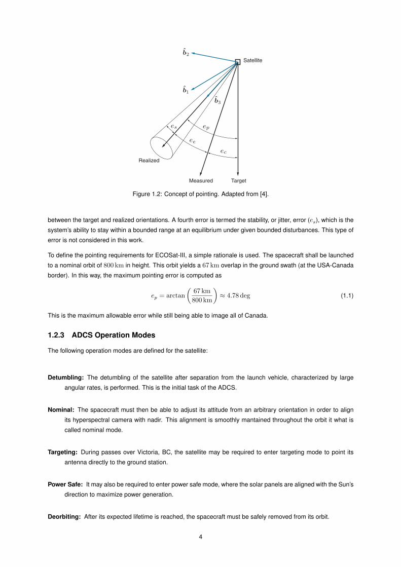
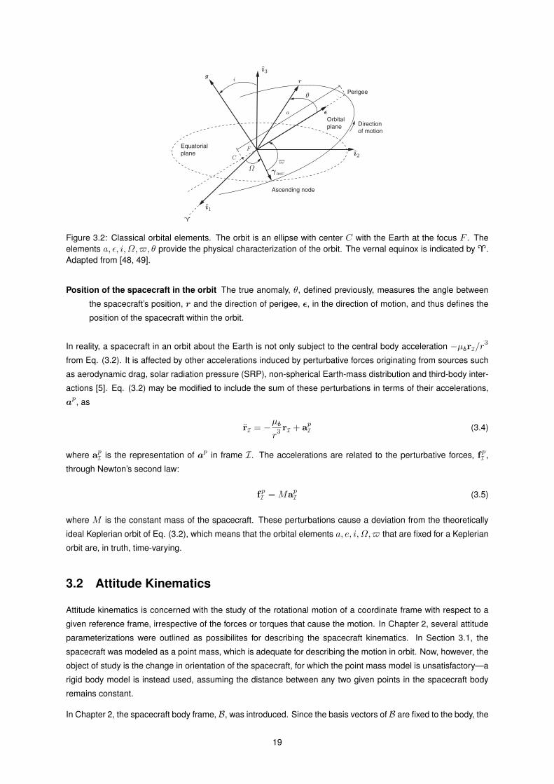
Figure 3.1: Geometry of a spacecraft in an elliptical orbit about the Earth with semi-major axis a, semi-minor axisb, semi-latus retum l and eccentricity ε < 1. Adapted from [49].

the orbital plane is defined by the following relation [49]:

r(θ) =l

1 + ε cos θ(3.3)

where ε ≡ ‖ε‖ is the norm of the eccentricity vector, or Laplace vector, ε, l is a constant geometric parameter

termed the semi-latus rectum, and θ is the angle between r and ε. The shape defined by the orbit equation, Eq.

(3.3), is a conic section with one of its foci at the center of the Earth. The parameter l previously introduced is

the length of the chord drawn from the focus to the trajectory. It has a semi-major, a, whose geometrical meaning

is dependent on the eccentricity, ε. For ε < 1, the orbit is an ellipse, with a, l > 0, as it can be seen in Figure

3.1. In this case, a is one half of the line segment that runs through both foci, connecting the point of minimum

separation of the two bodies, the perigee, to the point of maximum separation of the two bodies, the apogee2.

The semi-minor axis, b is the line segment at a right angle with a with one end at the center of the ellipse. The

circle is a particular case of the ellipse with ε = 0 and r = a = l. Elliptic orbits are the only closed orbits and are

therefore the only type of orbit featured in this work, contrary to parabolic (ε = 1, 1/a = 0) and hyperbolic (ε > 1,

a < 0) ones [49].

The Cartesian position and velocity are convenient to use for computational applications but provide little intuitive

understanding of the overall features of the orbit [48]. A total of six parameters are required to fully define the

spacecraft’s orbit in three-dimensional space: two for the orbit size and shape, two for the orientation of the orbital

plane in space, one for the orientation of the orbit within the plane, and one for the position of the spacecraft within

the orbit. These are represented in Figure 3.2 and described as follows.

Orbit size and shape The size and shape of a Keplerian orbit are fully defined by the semi-major axis, a, and

the eccentricity, ε, introduced previously.

Orientation of the orbital plane The inclination, i, is defined as the angle between the orbital plane and a given

reference plane (the equatorial plane for Earth satellites [48, 49]). The line of nodes is the intersection of

the orbital and equatorial planes and the ascending node designates the point on the line of nodes where

the orbit crosses the equatorial plane from the south to the north. The vector γasc specifies the position of

the ascending node with respect to the Earth’s center of mass (see Figure 3.2). Then, the second degree

of freedom to orient the orbital plane is defined by the right ascension of the ascending node (RAAN), Ω,

which is the angle between γasc and the vernal equinox, à, introduced in Chapter 2.

Orientation of the orbit within the plane This is equivalent to specifying the orientation of the major axis, or

line of apsides, within the orbital plane. This is accomplished by defining the argument of perigee, $,

which is the angle between γasc and the eccentricity vector (which defines the direction of perigee), ε,

measured in the direction of the spacecraft’s motion.

2Given the subject of this thesis, this chapter was developed for the case of a satellite orbiting the Earth. However, the theory is valid forany body orbiting a given primary, for which general case the terms “periapsis” and “apoapsis” apply.

18

gr

ϓ

i

a

Equatorial

planeF

C

Ascending node

Perigee

Orbital

plane Direction

of motion

ǫ

θ

Ω

ı1

ı2

ı3

γasc

Figure 3.2: Classical orbital elements. The orbit is an ellipse with center C with the Earth at the focus F . Theelements a, ε, i, Ω,$, θ provide the physical characterization of the orbit. The vernal equinox is indicated by à.Adapted from [48, 49].

Position of the spacecraft in the orbit The true anomaly, θ, defined previously, measures the angle between

the spacecraft’s position, r and the direction of perigee, ε, in the direction of motion, and thus defines the

position of the spacecraft within the orbit.

In reality, a spacecraft in an orbit about the Earth is not only subject to the central body acceleration −µÊrI/r3

from Eq. (3.2). It is affected by other accelerations induced by perturbative forces originating from sources such

as aerodynamic drag, solar radiation pressure (SRP), non-spherical Earth-mass distribution and third-body inter-

actions [5]. Eq. (3.2) may be modified to include the sum of these perturbations in terms of their accelerations,

ap, as

rI = −µÊr3

rI + apI (3.4)

where apI is the representation of ap in frame I. The accelerations are related to the perturbative forces, fpI ,

through Newton’s second law:

fpI = MapI (3.5)

where M is the constant mass of the spacecraft. These perturbations cause a deviation from the theoretically

ideal Keplerian orbit of Eq. (3.2), which means that the orbital elements a, e, i, Ω,$ that are fixed for a Keplerian

orbit are, in truth, time-varying.

3.2 Attitude Kinematics

Attitude kinematics is concerned with the study of the rotational motion of a coordinate frame with respect to a

given reference frame, irrespective of the forces or torques that cause the motion. In Chapter 2, several attitude

parameterizations were outlined as possibilites for describing the spacecraft kinematics. In Section 3.1, the

spacecraft was modeled as a point mass, which is adequate for describing the motion in orbit. Now, however, the

object of study is the change in orientation of the spacecraft, for which the point mass model is unsatisfactory—a

rigid body model is instead used, assuming the distance between any two given points in the spacecraft body

remains constant.

In Chapter 2, the spacecraft body frame, B, was introduced. Since the basis vectors of B are fixed to the body, the

19

kinematic equations of motion of the spacecraft are specified by the time-dependent relationship between B and

a reference. This reference is taken to be the ECI frame, I. This assumption will also be used for the dynamic

equations of motion in Section 3.3. Denote ω ≡ ωB/I as the angular velocity vector of frame B with respect to I.

Then, the kinematic differential equation for the DCM ABI that maps a rotation from I to B is given by

ABI (t) = − [ωB(t)×] AB

I (t) (3.6)

where ABI is the time derivative of AB

I , ωB ≡ ωB/IB = [ω1 ω2 ω3]T is the representation of ω in B and [ωB×]

is computed according to Eq. (A.22). Eq. (3.6) is the fundamental equation of attitude kinematics [5, 50]. This

relation can also be written in terms of the quaternion as [5]

qBI (t) =1

2ωB(t)⊗ qBI (t) (3.7)

Applying Eq. (2.14) to Eq. (3.7) gives

qBI (t) =1

2Ω [ωB(t)] q

BI (t) =

1

2Ξ[qBI (t)

]ωB(t) (3.8)

with

Ω(ωB) ≡[− [ωB×] ωB

−ωTB 0

](3.9)

and Ξ(qBI ) given by Eq. (2.15).

A significant advantage of the quaternion parameterization is that the kinematic equation, Eq. (3.8), is linear in

the quaternion. This, associated to the other advantages outlined in Chapter 2 and to the immense popularity of

the quaternion in attitude determination and control works, makes the quaternion the parameterization of choice

for the attitude in this master’s thesis.

3.3 Attitude Dynamics

In the previous section, the attitude motion was described in terms of the angular velocity, ω, of the body frame Bfixed to the spacecraft with respect to an inertial reference frame, I. Attitude dynamics tends to the determination

of this angular velocity by studying the moments, or torques, applied to the spacecraft.

Euler’s second law of motion for a rotating frame of reference states [46]

h+ ω × h = τ (3.10)

where h is the spacecraft’s angular momentum about its own center of mass, h is the temporal derivative of h

evaluated in the rotating frame of reference B and τ is the net applied moment about the center of mass. A

simple expression for h is given by

h = J ′ · ω (3.11)

The quantity J ′ is the second moment of inertia tensor of the rigid body with respect to its center of mass, defined

as

J ′ ≡∫

[(ρ · ρ) I − ρρ] dm (3.12)

20

where the integration is computed over the rigid body of the spacecraft (S/C), ρ is the position of an element of

mass dm with respect to the center of mass, ρρ is the dyadic product of ρ with itself and I is the identity tensor.

J ′ is typically time-varying. Its representation in the body frame, however, is constant [46]. It is therefore useful

to write the equation of dynamics in the B-frame. Then, Eq. (3.10) becomes

hB + [ωB×] hB = τB (3.13)

Inserting Eq. (3.11) in Eq. (3.13), noting that J′B = 0, yields

J′B ωB = − [ωB×] J′BωB + τB (3.14)

where ωB is the time-derivative of the representation of ω in frame B. J′B is termed the matrix of inertia of the

spacecraft about its center of mass expressed in the body frame. It is a symmetric and positive-definite matrix

computed as [46]

J′B ≡∫ (

ρTB ρBI3 − ρBρTB)

dm (3.15)

where ρB is the representation in frame B of ρ defined previously.

In some cases, the modeling of spacecraft as a single rigid body is insufficient to describe dynamical motion.

A more complex model consists in analyzing the spacecraft as a number of rigid bodies connected by joints

and having several degrees of rotational freedom. Some of these bodies may generate internal torques. In

contrast to external torques, internal torques result in, or are a result of, the exchange of angular momentum

between components of the spacecraft without changing the net system momentum [5]. Internal torques can be

generated by control mechanisms, such as reaction wheels, to change the orientation of the spacecraft.

Consider now the case of a system composed of the spacecraft and a RWS (S/C + RWS) consisting of K axially

symmetric reaction wheels about their spin axis. The i-th reaction wheel rotates about its spin axis, wwi with

a rotor spin rate ωwi with respect to frame B. Its moment of inertia about the spin axis is Jsi and its moment

of inertia about any axis transverse to the spin axis is J ti . Let W = ww1 , w

w2 , · · · , ww

K be a reference frame

whose coordinate axes are the spin axes of each reaction wheel. Then, a 3×K distribution matrix Ww is defined

as

Ww =[ww

1 ww2 · · · ww

K

](3.16)

where wwi ≡ (ww

i )B is the spin axis of the i-th wheel resolved in frame B. The total angular momentum of the

system about its center of mass represented in the B-frame is now given by [46]

hB = JBωB + hwB (3.17)

Now, JB is the moment of inertia matrix of the system with respect to the center of mass represented in the

B-frame, defined as [51]

JB = J′B +

K∑

i=1

J ti(ww′i

)B

(ww′i

)TB + J ti

(ww′′i

)B

(ww′′i

)TB (3.18)

where J′B is the moment of inertia matrix of the S/C without the RWS as defined in Eq. (3.15) and(ww′i

)B ,(ww′′i

)B

are any two vectors resolved in the B-frame perpendicular to wi and to each other3.3Eq. (3.18) is a particularization of the general case of a system with variable speed control moment gyros (VSCMGs), i.e. actuators that

consist in a reaction wheel mounted on a gimbal whose spin axis is perpendicular to the flywheel’s spin axis wwi , allowing it to tilt with respect

to B. The third axis completes the right-handed triad. For a RWS, there is no gimbal, so if the flywheel is axially symmetric, then wwi is the

only fully defined axis.

21

The term hwB is the angular momentum with respect to the center of mass of the system resolved in B generated

by the RWS when the wheels are spinning, which is equal to

hwB = Ww[hw1 hw2 · · · hwK

]T(3.19a)

hwi = Jsi

[ωwi + (ww

i )T ωB

], i = 1, 2, . . . ,K (3.19b)

Inserting Eq. (3.17) in Eq. (3.13) yields the dynamic equation of motion of a S/C + RWS system:

JB ωB = − [ωB×] (JBωB + hwB )− hwB + τB (3.20)

where

hwB = Ww[hw1 hw2 · · · hwK

]T(3.21a)

hwi = Jsi

[ωwi + (ww

i )T ωB

]≈ Jsi ωwi , i = 1, 2, . . . ,K (3.21b)

is the torque generated by the RWS. As expected, this torque generates an opposite reaction in the system—a

momentum exchange—hence the minus sign in Eq. (3.20). The term dependent on ωB in Eqs. (3.21) is generally

small and does not significantly impact the evolution of the wheel speeds, so it can be set to zero [52]. It becomes

clear that the matrix of inertia of the system, as defined by Eq. (3.18), does not include any term dependent on

the wheel speed inertia, Jsi , as that contribution is contained in hwB .

Denoting the RWS torque as τw and separating the external torques into external perturbations, τ p, and external

control torques, τ c, represented in B as

τwB ≡ hwB , τB ≡ τpB + τcB (3.22)

then Eq. (3.20) takes the form

JB ωB = − [ωB×] (JBωB + hwB )− τwB + τpB + τcB (3.23)

3.4 Spacecraft Perturbations

Spacecraft perturbations are defined as any contribution to the terms apI and τpB in Eqs. (3.4) and (3.23), respec-

tively. The former are called perturbative accelerations, which are induced by perturbative forces, while the latter

are perturbative torques. Perturbative forces cause a time-variation in the orbital elements, as mentioned in Sec-

tion 3.1, causing the orbit to deviate from a Keplerian model. Perturbative torques cause a unintentional change

in the angular rate of the spacecraft. In this section, perturbative forces and torques that affect the spacecraft are

discussed and modeled.

3.4.1 Perturbative Forces

Perturbative forces which modify simple Keplerian orbits may be divided into four classes: nongravitational forces,

third-body interactions, nonspherical mass distributions and relativistic mechanics [38, 53]. The primary non-

gravitational forces consist of aerodynamic drag and solar radiation pressure. For most applications relativistic

mechanics may be completely neglected and for spacecraft in low Earth orbit (LEO) third-body interactions are

not significative [38]. As such, these effects will not be modeled.

22

Aerodynamic Drag

Drag is a hindering force due to atmospheric friction and with a direction opposite to the spacecraft’s velocity.

Since the density of the atmosphere, to which drag is proportional, decreases exponentially with an increase

in altitude, the effects of this perturbation are more severe at the perigee of the orbit. As the drag slows the

spacecraft at each perigee passage, the apogee height and, consequently, the semi-major axis and eccentricity

are reduced. The perigee height and argument of perigee remain approximately the same [38].

To model the aerodynamic drag force acting on the spacecraft, the following assumptions are made [46]: the

momentum of molecules arriving at the surface is totally lost to the surface; the mean thermal motion of the

atmosphere is much smaller than the speed of the spacecraft through the atmosphere; momentum transfer

from molecules leaving the surface is negligible; and for spinning vehicles, the relative motion between surface

elements is much smaller than the speed of the mass center.

The expression for the aerodynamic drag force acting on the spacecraft is given by

fa =

∫H(cosα)ρa

(vR)2

cos(α)dAvR (3.24)

where vR ≡ ‖vR‖ and vR ≡ vR/vR is a unit vector in the direction of vR and H(x) is the Heaviside function.

Here, vR is the velocity of the local atmosphere relative to a surface element of the spacecraft dA such that

vR = vcR − ω × ρ (3.25)

where vcR is the velocity of the atmosphere with respect to the spacecraft’s center of mass, ω is the angular

velocity of the spacecraft body frame B relative to I and ρ now locates dA with respect to the spacecraft’s center

of mass. The quantity ρa is the density of the local atmosphere and α is the angle of attack defined as

cosα = vR · nA (3.26)

where nA is a unit inward normal to the surface at dA. The computation of Eq. (3.24) depends on the spin of the

spacecraft. If the spacecraft is not spinning, then vR is constant over the surface, as seen from Eq. (3.25), and

the aerodynamic force represented in the B-frame is given by

faB =[ρa(vR)2Ap

]vRB (3.27)

where vRB is the representation of vR in B and the integral defined as

Ap ≡∫H(cosα) cos(α)dA (3.28)

is the total projected area seen by the atmospheric flow. If the spacecraft is rotating, the aerodynamic force is

instead

faB = ρavcRAp

[vcR − (caB)

T ωB

]vcRB + [cpB×] ωB

(3.29)

where vcR ≡ ‖vcR‖, vcR ≡ vcR/vcR and vcRB is the representation of vcR in B. The quantities cpB and caB are the

representations of the pressure and aerodynamic centers in frame B, respectively, defined as

cpB ≡1

Ap

∫H(cosα) cosαρB dA, caB ≡

1

Ap

∫H(cosα) [ρB×] dAB (3.30)

23

with dAB defined as

dAB ≡ nABdA (3.31)

where nAB is the representation in frame B of the unit normal nA. The aerodynamic drag-induced acceleration aaB

can then be computed through Newton’s second law, Eq. (3.5).

Nonspherical Mass Distribution

The Earth’s rotation about its axis accounts for its equatorial bulge and flattening at the poles. Indeed, the Earth is

not exactly spherically symmetric, but rather has an approximate configuration of an oblate spheroid with a polar

radius 21.4 km larger than its equatorial one. Besides this, it has a superficial pear-like shape at the equator and

several minor mass anomalies (i.e. continents and mountains) [48].

The oblateness of the Earth causes an effect termed the regression of the nodes, which is the motion of the line

of nodes opposite the direction of the spacecraft’s motion. The other main oblateness perturbation is the motion

of the line of apsides. This is equivalent to a cumulative, secular variation of the elements $ and Ω, while a, e,

and i undergo short period variations that average to zero over an orbit [38].

Due to the conservative nature of the gravitational field, the vector form of Eq. (3.2) may be rewritten as the

gradient of a scalar potential [38]:

r = −∇U (3.32)

where r is the acceleration suffered by the spacecraft in orbit with respect to the mass center of the Earth and

∇U is the gradient of the potential function U . Due to the approximate spherical symmetry of the Earth, it is

convenient to develop the expression for U in spherical coordinates. To this end, let rS = [r φ ψ]T denote

the position of the spacecraft in the rotating frame S. Then, U is expressed as

U = −µÊr

+B(r, φ, ψ) (3.33)

where −µÊ/r is the Newtonian gravitational potential that leads to Eq. (3.2) in its ideal, Keplerian form and

B(r, φ, ψ) is the spherical harmonic expansion that corrects the previous term for the Earth’s asymmetric mass

distribution, given by [54]

B(r, φ, ψ) =µÊr

[ ∞∑

n=2

Jn

(RÊ

r

)nPn(sinφ) +

∞∑

n=2

n∑

m=1

Jnm

(RÊ

r

)nPnm(sinφ) cosm(ψ − ψnm)

](3.34)

Here, r, φ and ψ are the spacecraft’s radius, latitude and longitude. RÊ is the mean equatorial radius of the Earth.

The quantities Jn, Jnm and ψnm are numerical coefficients. The functions Pn(x) and Pnm(x) are Legendre’s

polynomial of degree n and the associated Legendre function of degree n and order m, respectively. The terms

related to Legendre’s polynomials constitute the zonal harmonics, which describe deviations in the north-south

direction of the potential from the Newtonian one. The terms having Jnm, n 6= m, as factors are the tesseral har-

monics; those having Jnm, n = m, are the sectorial harmonics. The tesseral and sectorial harmonics represent

deviations in an east-west direction [54]. By far, the strongest perturbation due to the shape of the Earth arises

from the J2 zonal coefficient, which is closely related to the oblateness of the Earth [54], with J3 being more than

400 times smaller [5].

Taking the gradient of U in spherical coordinates in Eq. (3.32) yields the inertial perturbative acceleration due to

24

the non-spherical Earth represented in frame S as

agS =

[−∂B∂r

−1

r

∂B

∂φ− 1

r sinφ

∂B

∂ψ

]T(3.35)

The perturbative acceleration represented in frame I is obtained with the rotation matrices defined in Chapter 2:

agI = AIFA

FS a

gS (3.36)

Solar Radiation Pressure

Solar radiation pressure affects the spacecraft through momentum exchange between the spacecraft and photons

incident on its surface. Contrary to aerodynamic drag, SRP only contributes at times when the spacecraft is not

in eclipse. Solar radiation pressure causes periodic variations in all of the orbital elements [53].

To model the SRP acting on the spacecraft, the following assumptions are made [46, 5]: the momentum of

photons arriving at the surface is totally absorbed by the surface; the force due to thermal radiation emitted from

the spacecraft is ignored; the Sun is the only source of radiation interacting with the spacecraft; the spacecraft’s

self-shadowing is ignored; and for spinning vehicles, relative surface velocities are negligible when compared to

the speed of light.

The pressure of radiation originating from the Sun is essentially constant in the vicinity of the Earth and equal to

pÊ. The force exerted on the spacecraft body due to pÊ is [46]

fs = −pÊAps (3.37)

where s is a unit vector pointing from the spacecraft in the direction of the Sun (the Sun line-of-sight vector) and

Ap is given by Eq. (3.28) with α now defined as

cosα ≡ −s • nA (3.38)

where nA is the inward unit normal to the surface element dA. Eq. (3.37) is written in body frame components

directly as

fsB = −pÊApsB (3.39)

The result given in Eq. (3.39) is resolved in the B-frame, so it needs to be mapped using the DCM from B to I,

AIB = (AB

I )T . Then, the SRP-induced acceleration asI in the ECI frame is then computed using Eq. (3.5).

3.4.2 Perturbative Torques

Perturbative forces may be classified as being either internal or external. Internal perturbative torques are typically

caused by the pointing rotation of solar arrays, antennas or cameras; the deployment of antennas, solar arrays,

instruments or booms; propellant slosh; flexible appendages; and reaction wheel imbalances. They are generally

much smaller than the external torques, needing to be accounted for in high-precision pointing systems [55]. As

such, they are not modeled in this work. The principal external torques acting on a spacecraft are the gravitational

torque, the aerodynamic torque, the SRP torque and the magnetic torque [46].

25

Aerodynamic Torque

To compute the aerodynamic torque, the same assumptions that where used to model the aerodynamic force

(Subsection 3.4.1) are used. The expression for the torque is given by [46]

τ a =

∫H(cosα)ρa

(vR)2

cos(α)ρdA× vR (3.40)

where vR is the velocity of the local atmosphere relative to dA given by Eq. (3.25), vR is its norm and vR is a

unit vector pointing in its direction; α is given by Eq. (3.26); H(x) is the Heaviside function; ρ is the position of

dA with respect to the center of mass; and ρa is the density of the local atmosphere. When the spacecraft is not

rotating, the expression for the torque in components of frame B becomes

τaB = ρa(vR)2Ap [cpB×] vR

B (3.41)

where Ap is the integral given by Eq. (3.28), cpB is the center of pressure defined by Eq. (3.30) and vRB is the

representation of vR in frame B.

If the spacecraft is rotating, then Eq. (3.40) instead becomes

τaB = ρavcR[vcRAp [cpB×] vcR

B −(JAB +

[vcRB ×]JA′

B

)ωB

](3.42)

where vcRB is the unit vector in the direction of vcR represented in B, the velocity of the atmosphere with respect

to the spacecraft’s mass center, and vcR is the norm of vcR; ωB is the representation in B of the angular velocity

of B with respect to I; and the geometrical integrals JAB and JA′

B are given by

JAB ≡

∫H(cosα)

(ρTB ρBI3 − ρBρTB

)cosα dA (3.43)

JA′

B ≡∫H(cosα)ρB dAT

B [ρB×] (3.44)

where ρB is the representation in frame B of ρ and dAB is defined in Eq. (3.31).

Gravity Gradient Torque

The non-uniformity of the gravitational field over a rigid body in space leads to a torque about its mass center.

This effect is termed the gravity gradient affecting the spacecraft. In order to model this torque, the following

assumptions are taken [46]: only the influence of the Earth as a primary needs to be considered; the Earth

possesses a spherically symmetrical mass distribution; the spacecraft is small compared to its distance from the

mass center of the Earth; and the spacecraft consists of a single body.

Indeed, contrary to what was done in Subsection 3.4.1 for the modeling of the non-spherical mass distribution

force, the Earth is assumed to have a spherically symmetrical mass distribution for gravity gradient torque con-

siderations. This assumption is valid considering the magnitude of the gravity gradient torque compared to the

magnitude of the other external torques [38].

The expression for the gravity gradient torque is given directly in frame B by [46]

τgB = 3

(µÊ

r3

)[(o3)B×] JB(o3)B (3.45)

where where µÊ is the standard gravitational parameter of the Earth, r is the distance from the center of the Earth

26

to the center of mass of the spacecraft, JB is the inertia matrix of the spacecraft in components of frame B and

(o3)B is the representation of o3 in frame B, i.e. the third column of the DCM ABO from frame O to B.

Solar Radiation Pressure Torque

To model the torque caused by SRP, the same assumptions as those made in Subsection 3.4.1 are taken for the

SRP force. The torque expressed in components of frame B is given by the cross product between the center

of pressure, cpB, defined in components of B in Eq. (3.30) with α given by Eq. (3.38), and the SRP force, fsB ,

expressed in components of B in Eq. (3.39) [46]:

τsB = −pAp [cpB×] sB (3.46)

where p is the pressure of solar radiation, Ap is given by Eq. (3.28) and sB is the unit vector pointing from the

spacecraft in the direction of the Sun represented in B.

Magnetic Torque

The Earth generates a magnetic field which interacts with spacecraft in its vicinity. When the spacecraft has a

magnetic moment, m, this interaction translates in to a torque mechanism expressed by [46]

τm = m× ζ (3.47)

where ζ is the external magnetic flux density. The magnetic moment m is the net magnetic moment of the

spacecraft. Sources that contribute to m include permanent magnets, current loops, electronic systems and

scientific instruments [46].

Similarly to the gravitational potential described in Subsection 3.4.1, the magnetic flux density generated by the

Earth may be computed through the gradient of a scalar potential [46]:

ζ = −∇V (3.48)

The scalar potential V may be written as [56]

V (r, φ, ψ) = RÊ

[ ∞∑

n=1

n∑

m=0

(gnm cosmψ + hnm sinmψ)

(RÊ

r

)n+1

Pnm(cosφ)

](3.49)

where r, φ, ψ are the spacecraft’s radius, latitude and longitude, respectively; R is the mean equatorial radius of

the Earth; gnm, hnm are termed Gauss coefficients and describe internal sources; and Pnm(x) is the associated

Legendre function. The accuracy of the model will depend on this order and degree n,m to which Eq. (3.49) is

computed, which is done numerically.

Taking the gradient of V in spherical coordinates in Eq. (3.48) yields the magnetic flux density generated by the

Earth represented in frame S as

ζS =

[−∂V∂r

−1

r

∂V

∂φ− 1

r sinφ

∂V

∂ψ

]T(3.50)

Then, the magnetic torque represented in frame B is given by

τgB = [mB×] ABS ζS (3.51)

where mB is the representation of m in frame B and ABS = AB

EAES is the DCM from frame S to frame B.

27

Chapter 4

Sensor and Actuator Hardware

In this chapter, the ADCS is analyzed from the perspective of hardware. In Section 4.1, characteristic examples of

spacecraft sensors are outlined. Sensors are employed to carry out attitude measurements, i.e. the measurement

of a quantity that contains information relative to the orientation of the S/C. These can be, for example, the

magnetic field flux density vector ζ, the direction of the Sun s (or another celestial body); or the angular rate

of the spacecraft ω. In Section 4.2, the actuators that allow for the control of the spacecraft are discussed. In

Section 4.3, an adequate sensor and actuator suite for ECOSat-III that will allow the fulfillment of the mission

objectives planned in Chapter 1 is selected based on the previous sections.

4.1 Sensors

Attitude determination requires a combination of both sensors and mathematical models. Depending on the

nature of the performed measurement, sensors may be divided into two categories: reference sensors and

inertial sensors [28].

Reference sensors produce vector observations in the satellite body-fixed frame with respect to certain known

references. They are called absolute attitude measurements [57]. These vector observations may be unit vectors

in the case when only a direction is measured, as is the case with Sun sensors (SSs), Earth horizon sensors

or star sensors. However, they may also measure a magnitude, such as a magnetometer used to measure

the local geomagnetic field. Let z be a certain three-dimensional vector. A reference sensor would measure

the components of z in the body frame, zB, while a mathematical model is used to determine the reference, or

inertial, direction, zI . The vector z can be, for instance, the Sun vector s. In this case, a Sun sensor produces

a measurement zB of s, while the reference zI is computed with resort to planetary ephemerides. An attitude

determination algorithm is then employed to find a rotation matrix ABI , or equivalent parametrization, such that,

ideally zB = ABIzI .

Note that a sensor does not necessarily produce a line-of-sight (LOS) measurement directly. Indeed, Sun sen-

sors convey information on the three components of s in the body frame by measuring two spatial angles [58].

However, any reference sensor output may be converted into vector form in what is known as the LOS measure-

ment model, which is the most widely used observation equation in attitude determination [59]. As such, this

section does not intend to expand upon sensor mathematical models as it is assumed that every measurement

is obtained in such form.

As indicated in Chapter 2, three independent parameters define the attitude. However, the magnitude of a vector

has no information relevant to attitude determination, so any absolute attitude measurement bears a unit-norm

constraint and contains only two independent scalar pieces of attitude information [10]. The problem of attitude

determination is then unique in the sense that it is both underdetermined, as one measurement is not enough,

and overdetermined, as two measurements is too many [60]. As a result, it is required to have at least two

non-collinear measurements (static attitude determination) or to incorporate previous information from the past

(recursive attitude determination). Recursive attitude determination is the subject of Chapter 5.

28

When considering the latter approach, some knowledge of system dynamics is required to propagate attitude

information from the past to the current time [10]. This can be done, for instance, with the inclusion of an

inertial sensor, namely a gyroscope. Inertial sensors measure motion relative to an inertial frame; gyroscopes,

in particular, provide angular rates by integrating the sensed angular acceleration. This integration generates a

drift, which is why the information provided by them must be updated by reference sensors [10, 15].

4.1.1 Inertial Sensors

Inertial sensors measure linear acceleration or angular velocity. The former are called accelerometers, while

the latter are termed gyroscopes. Accelerometers are typically used to complement a propulsion system and

therefore are not discussed in this work [14]. Gyros used in spacecraft ADCS are typically divided into two

categories: rate gyroscopes (RGs) and rate-integrating gyroscopes (RIGs) [38].

Rate gyros directly measure the spacecraft angular velocity, or rate, about a fixed axis with respect to an inertial

frame. Rate-integrating gyros, on the other hand, measure integrated rates or angular displacements [5]. They

can also be classified by the physical mechanisms they use: spinning mass gyros, optical gyros and vibrating

gyros [61]. Spinning mass gyros have a mass of controlled rotational speed and known moment of inertia that is

spinning steadily about an axis. The rotation of the mass tends to keep the direction of its spin axis constant. A

rotational input to the gyro, other than in the spin axis, caused by the turn of the spacecraft generates a predictable

rotational response in an expected output axis, a process termed gyroscopic precession. Optical gyros are based

on the Sagnac effect which states that the phase shift between two waves originating from the same light source

but propagating in opposite directions inside in a rotating ring interferometer is proportional to the angular velocity

of the ring. Lastly, vibrating gyros are dependent on the Coriolis effect to determine the angular rate: the spinning

wheel is replaced with a vibrating body that is acted upon by torques when subject to Coriolis accelerations. By

measuring the amplitude of the resulting vibration, the angular rate is determined.

MEMS Gyroscopes

The integration of conventional gyros in CubeSat structures is troublesome due to the tight constraints in size,

weight and power. The miniaturization of spinning mass gyros itself is quite difficult, which is currently leading to

their decline and consequent market opening for optical and vibrating gyros that can be effectively made smaller

[61]. This lead to the development of micro-electromechanical systems (MEMS) gyros, which are miniaturized

vibrating angular rate sensors. Silicon and quartz-based MEMS gyros have a reduced cost, size, weight and

power consumption and, unlike inertial-grade and some tactical-grade gyros, are commercially available devices

with a broad range of applications, including traction control systems in automobiles, gaming consoles, anti-jitter

systems in digital cameras and wireless 3D pointing devices [61]. Altough bearing the aforementioned desired

characteristics, MEMS gyros also have a lower performance and shorter lifetime compared to other gyros [5].

4.1.2 Reference Sensors

Sun Sensors

Sun sensors measure the direction of the sun relative to the spacecraft. They are the most widely used sensor

type, as the Sun is sufficiently bright to allow them to be simple, reliable and have minimal power requirements; in

addition, many missions rely on thermal or power constraints related to the Sun and, consequently, are concerned

with the orientation and evolution in time of the Sun vector in body coordinates [38].

There are three basic classes of Sun sensors: analog sensors, Sun presence or coarse sensors, and digital sen-

sors. Analog Sun sensors are composed of silicon solar cells, or photocells, whose output current is proportional

to the cosine of the angle of incidence of the solar radiation. For this reason, analog sensors are frequently called

29

cosine detectors. A mask can be applied to shadow a portion of one or more photocells which can be configured

to yield a two-axis sensor. Coarse Sun sensors (CSSs) generate a step function response that indicates when

the Sun is within the field-of-view (FOV) of the detector. These are typically employed as a crude method to easily

determine if a part of the S/C is sunlit so as to protect on-board instrumentation or position the S/C for an experi-

ment. They are also used to activate hardware. Digital Sun sensors (DSSs) have a superior accuracy to analog

Sun sensors and CSS arrays and are typically composed of two parts: a command unit and a measurement unit.

The command unit is a Sun-presence detector composed of two slits and a photocell and the measurement unit

provides a digital output which is a representation of the Sun incidence angle with respect to the sensor face nor-

mal when the Sun is in the FOV of the command unit. Two-axis DSSs consist of two measurement components

mounted at right angles.

Magnetometers

Magnetometers are sensors that provide both the direction and magnitude of the magnetic field. Along with Sun

sensors, magnetometers are extensively used in ADCS in particular for the readiness associated with vector

sensing, as well as their reliability, light weight, low power requirements, operation over a wide temperature range

and the fact that they have no moving parts [38]. Magnetometers require a magnetic field model to predict the field

direction and magnitude at the spacecraft’s position, which essentially limits their use in attitude determination to

LEO [5].

Other Reference Sensors

As discussed, Sun sensors and magnetometers are among the most universally utilized attitude determination

sensors. Other more complex and expensive sensors include Earth horizon sensors, star trackers and Global

Positioning System (GPS) receivers.

Earth horizon sensors, or simply horizon sensors, detect points on the Earth’s horizon. Multiple points can then

be used to compute the nadir vector. Horizon sensors can be of two types: static sensors that look in fixed

directions and scanning sensors that bear a detector with a moveable FOV across the Earth [5].

Star trackers are digital cameras with a focal plane consisting of CCD or CMOS pixels [5]. These sensors measure

the coordinates of stars in the body frame which are then compared with known directions obtained from a star

catalog or almanac. Star trackers are generally the most accurate attitude sensors, attaining accuracies up to

the arc-second range. However, they come with a considerable cost, being heavy, expensive and requiring more

power than most attitude sensors [38].

Attitude information is contained in the phase difference between a GPS wave received by two spatially separated

antennas. The achievable accuracy is dependent on the precision to which the phase can be measured [10]. The

use of GPS receivers for attitude determination is not yet very widespread and is currently a complimentary

technology used to provide reliable velocity and positioning information. However, the integration of GPS data

is becoming a solid method in correcting attitude information obtained from MEMS-based inertial measurement

units (IMUs) [62].

4.2 Actuators

In this section, a review of spacecraft control actuators is done. Two main actuators, momentum/reaction wheels

and magnetorquers, are highlighted. Other spacecraft actuators are also briefly reviewed.

30

4.2.1 Momentum and Reaction Wheels

Momentum wheels and reaction wheels are structures composed of a rotating flywheel, a wheel or disk used

to store or transfer momentum; an internal brushless DC electric motor; and associated electronics [5]. As

introduced in Chapter 3, reaction wheels (and also momentum wheels) generate internal torques, which means

that the net system momentum stays constant during their operation.

The fundamental difference between a momentum wheel and a reaction wheel is in the mode of operation.

Some sources use the convention that a momentum wheel is designed to operate at a biased momentum, while

a reaction wheel is designed to operate at zero bias [38]. However, reaction wheels seldom operate around

null reference speed rates as they exhibit a non-linear response in that neighborhood due to friction, causing

an irregular motion of the spacecraft [50, 63]. This is solveable by running the reaction wheels with a “small”

reference bias, whereas the momentum wheels operate with a “large” reference bias; since the momentum

transfer is dependent upon the moments of inertia of the wheels and the spacecraft, the concepts of “small”

and “large” are ambiguous and the definition is not rigorous. A more suitable definition would be as follows.

Reaction wheels respond to disturbances on the spacecraft, i.e. a pointing error computed by the controller

creates a signal which speeds up the wheel from its nominal speed rate, correcting the orientation. RWSs are

used for three-axis stabilization and precision pointing setups, for which a minimum number of three flywheels

are necessary. Momentum wheels, on the other hand, are run at a nearly constant speed in order to provide

gyroscopic stiffness to the vehicle. These are employed for momentum bias stabilization, where often just one

flywheel is used with its spin axis mounted along the pitch axis, normal to the orbit plane [53].

When using a RWS to counter external perturbations, a periodic disturbance torque along one spacecraft axis

typically results in a cyclic variation in the angular rate of the wheel directed along that axis, while a secular

disturbance leads to a linear increase in angular rate, as the wheel would be accelerated at a constant rate in

order to transfer to it the excess angular momentum due to the external disturbance (see Eq. (3.21)). This is only

sustainable up to a physical limit for the spin rate of the wheel, termed the saturation speed. A process called the

desaturation of the wheels must be carried out, which consists in the generation of external torques, supplied by

an additional suite of actuators, so as to dump momentum from the spacecraft [64].

4.2.2 Magnetic Torquers

Magnetic torquers, or magnetorquers, are actuators that generate magnetic dipole moments. This magnetic

dipole mc interacts with the Earth’s local magnetic field according to Eq. (3.47) to yield a control torque τ c:

τ c = mc × ζ (4.1)

where ζ is the Earth’s magnetic field flux density. Eq. (4.1) shows that the magnetic control torque can only

be applied to the spacecraft in a plane orthogonal to the instantaneous direction of the Earth’s magnetic field.

This implies that the spacecraft is instantaneously underactuated if attitude control is done relying only in mag-

netometers. This is a strong deterrent for the use of magnetorquers as primary actuators in spacecraft and

they usually play a secondary role, such as the detumbling after launch and the momentum dumping of reaction

wheels [65]. However, magnetorquers do not require any propellant, have low power requirements, and have an

unlimited lifetime, as well as no moving parts. These features make them quite popular, simple to manufacture

and inexpensive actuators which are commonly featured as a primary system on CubeSats [50].

Magnetorquers are built from magnetic coils or electromagnets (rods) whose magnetic moment depends on the

number of coil windings, the cross-sectional area of the coil, and on the amount of current that passes through

the coil [50]

31

4.2.3 Other Actuators

Besides magnetorquers, other actuators that provide an external torque to the spacecraft are gas jets or thrusters.

These work by expelling propellant, creating thrust in the opposite direction. Thrusters not only produce torques,

but also generate forces and, besides being used for attitude control and momentum dumping, are used also to

control spin rates, nutation and to adjust obits. In LEO, either thrusters or magnetorquers can be used for many

of the same purposes and, despite providing larger torques, the propellant supply required for thrusters is a major

limitation on their use [38]; this is particularly restrictive for CubeSats, which fall under strict mass requirements.

With respect to momentum exchange, other actuators include control moment gyros (CMGs) and variable speed

control moment gyros (VSCMGs). A CMG consists in a flywheel mounted on a gimbal; the flywheel’s speed

is made constant but the gimbal allows the spin axis to rotate with respect to B. A VSCMG is a CMG where

the flywheel’s speed is also variable. These actuators are advantageous in the sense that the extra degree of

freedom makes it harder for the flywheel to saturate—or impossible in the case of CMGs. However, they often

bear highly complex control laws [51].

4.3 Hardware Selection

The design of the sensor and actuator suite for an ADCS is performed based on the mission requirements and

the trade-off process that needs to be taken into consideration when designing a satellite with strict limitations,

such as a CubeSat. While the principal actuator has been decided upon prior to this work, as the ECOSat-III

will feature reaction wheel actuators for enhanced pointing accuracy respective to ECOSat-II, the main challenge

of this sub-task lies in proposing an adequate sensor suite. When selecting sensors for a CubeSat design, one

must consider three main criteria: the available volume, the weight and the financial budget. The choice of this

selection must be thoroughly justified.

There is not a straightforward algorithm that yields the most adequate ADCS sensor selection. In fact, what is

usually done in the space industry is a more subjective approach: typically, one identifies candidate sensor suites

and conducts a trade study to determine the best, most cost-effective approach. In such studies, the existence of

COTS components and software can strongly influence the outcome. The selection is most directly influenced by

the required orientation of the spacecraft and its accuracy. Other influences include redundancy, fault tolerance,

field of view requirements, and available data rates. These provide some guidelines which aid to the selection

[53].

Table 4.1 describes the effects of payload pointing on the hardware selection process. Payload pointing not only

influences the class of sensors used, but also the number and kind of actuation devices and the control method.

In this case, the differences are categorized into whether the S/C is Earth-pointing (the target is somewhere

on Earth or scanning) or inertial pointing (Sun, other celestial targets). Since ECOSat-III’s payload shall be

pointed at a ground station, it classifies as Earth-pointing. Given this, it can be said that sensors such IMUs and

magnetorquers for momentum-dumping are adequate. Liberty to choose between horizon, Sun or star sensing

still exists and will be considered for trade-off.

Table 4.2 displays which sensors and actuators are adequate to use given the required precision. The first row

describes what is typically called coarse “sun-mag” attitude determination, relying on the use of sun sensors

and magnetometers to provide the two minimum vector measurements for absolute attitude determination. The

use of sun sensors has the problem of susceptibility to data loss in case of eclipse. IMUs such as gyros are

often included to provide relative attitude observations between measurements. To reach 1 deg accuracy, horizon

sensors are often employed. Star sensors only come into play when one desires an accuracy better than 1 deg.

Note that star sensors are much more expensive and consume more power than the other discussed sensors.

32

Table 4.1: Effect of payload pointing directions onADCS design for 3-axis controlled spacecraft. Adaptedfrom [53].

Requirement Effect on ADCS

Earth-pointing

horizon sensor for local vertical reference (pitchand roll)

Sun or star sensor for third axis

reaction wheels, momentum wheels or controlmoment gyros for accurate pointing

magnetorquers for momentum dumping

IMUs for maneuvers and attitude determination

Inertial-pointingtypically sun sensors, star-trackers and IMUs

typically reaction wheels and thrusters

Table 4.2: Effect of control accuracy on sensor selectionand ADCS design. Adapted from [53].

Requiredaccuracy(3σ) [deg]

Effect on ADCS

> 5major cost savings

Sun sensors and magnetometers adequate

1 - 5Sun sensors and horizon sensors adequate

Reaction wheels adequate

magnetorquers and magnetometers useful

0.1 - 1

star tracker or horizon sensors

gyros

reaction wheels

magnetorquers and magnetometers feasible for light S/C

< 0.1 star sensor needed

(a) CRS09-01 MEMS gyroscope (b) RM3100 magnetometer (c) NanoSSOC-A60 sun sensor

Figure 4.1: Selected sensors for ECOSat-III [66–68].

Regarding the sensor hardware, based on this analysis the safest approach would be to design a suite including

a gyro, a magnetometer, a Sun sensor and a horizon sensor. However, several points may be argued against the

inclusion of the latter. A horizon sensor is costly compared to the other three sensors, which are approximately

in the same category in terms of price. The addition of an horizon sensor would also increase substantially

the mass and volume of the CubeSat. It is therefore difficult to evaluate whether the extra precision gained

from including a horizon sensor is worth the negative impact. The required precision of 4.78 deg is quite close

to the 5 deg threshold of Table 4.2. In fact, recent CubeSat designs equipped with gyros, magnetometers and

Sun sensors from the last five year have performed quite well in terms of attitude determination performance,

obtaining results in terms of angular error ranging from 0.2 deg to 3 deg during the sunlit orbital phase and from

2 deg to a worst-case scenario of 18 deg during eclipse in the studied cases [22, 25, 28, 30–32]. The sensor

market is an evolving one and sensors for smallsats becoming smaller, more precise, less power consuming and

less expensive. Therefore, a reasonable choice for the first iteration of the ECOSat-III ADCS suite consists in a

gyro, a magnetometer and a Sun sensor.

With respect to the actuator suite, in addition to the RWS, it is clear from the analysis in this chapter that magne-

torquers are to be chosen to dump the momentum of the reaction wheels. Magnetorquers are also used for the

detumbling of the spacecraft, when the angular rates are too high for an effective control of the RWS.

Gyro: Silicon Sensing CRS09-01

The selected gyro for ECOSat-III is the Silicon Sensing CRS09-01 MEMS gyroscope. It is displayed in Figure

4.1a. Its main characteristics are displayed in Table 4.3 . It is one of the best commercially available MEMS

gyros [61], selected from a trade-off with three others: the Systron Donner QRS116, the Honeywell HG1900 and

the Analog Devices ADIS16135. Being a COTS equipment, it costs only 900 USD. This price is beaten by the

ADIS16135, which costs 200 USD less; however, the noise figures in the ADIS16135 were deemed too high for

33

Table 4.3: CRS09-01 characteristics[66].

Parameter Unit Value

Rate range deg s−1 ±200

Resolution deg h−1 27

Angle random walk deg h−1/2 0.1

Bias instability deg h−1 3

Rate random walk deg h−3/2 0.4323

Material - Silicon

Power supply V 5

Power consumption mA 100

Mass g 59

Cost USD 900

Table 4.4: RM3100 characteristics[67].

Parameter Unit Value

Field measurement range µT ±800

Resolution nT 13

Noise level nT 15

Power supply V 2

Power consumption mA 50

Mass (b2, b3-sensors) g 0.06

Mass (b1-sensor) g 0.09

Cost USD 61

Table 4.5: NanoSSOC-A60 charac-teristics [68].

Parameter Unit Value

Accuracy (3σ) deg 0.5

FOV deg ±60

Power supply V 5

Power consumption mA 2

Mass g 4

Cost USD 2360

(a) ISIS Space iMTQ MagnetorquerBoard (illustrative)

(b) Flywheel cross-section (c) 1202H006BH motor

Figure 4.2: Selected actuators for ECOSat-III [70].

this application, making it impossible to achieve the mission requirements. The other gyros considered in the

trade-study had prices in the order of thousands of dollars, which is very much above the ADCS budget. The

CRS09-01 was thus deemed the best choice for quality with respect to price.

Magnetometer: PNI RM3100

The three-axis magnetometer (TAM) used in this work is the PNI RM3100. It is displayed in Figure 4.1b. Its

main characteristics are displayed in Table 4.4. The RM3100 is the successor of the discontinued MicroMag3,

a magnetometer developed also by PNI which has a CubeSat flight legacy aboard the RAX-2 satellite, built

by the University of Michigan, and the Aeneas CubeSat, built by the University of Southern California. Other

magnetometers considered in the trade study have their cost in the order of hundreds of dollars; the RM3100

costs only 61 USD and has a similar performance to the other magnetometers considered.

Sun sensor: Solar MEMS Technologies NanoSSOC-A60

The two-axis sun sensor considered in this work is the Solar MEMS Technologies NanoSSOC-A60 analog sun

sensor for nano-satellites. It is displayed in Figure 4.1c. Its main characteristics are displayed in Table 4.5. Apart

from less precise photocells and in-house developed sensors, the SSBV sun sensor is the typical choice for

CubeSat sun sensing. However, Solar MEMS Techologies’ alternative NanoSSOC-A60 sensor costs 1000 USD

less, with a similar accuracy and a wider FOV. The digital edition, NanoSSoc-D60, was also considered. However,

it is 1500 USD more expensive than its analog counterpart. Adding a microcontroller with an analog-to-digital

converter (ADC) attached to the controller area network (CAN) bus to fit an analog sun sensor has essentially a

negligible cost compared to the alternative [69].

Magnetorquer: Custom-Built Torque Rods

ECOSat-III’s three-axis magnetorquer is constituted by six orthogonally-oriented magnetic torque rods, two per

axis. An illustrative example of a three-axis magnetorquer system constituted by two torque rods and one coil

34

Table 4.6: Magnetorquer characteristics for individual rods[71].

Parameter Unit b1-rods b2, b3-rods

Magnetic moment A m2 14.908 0.913

Turns per layer - 619 127

Number of layers - 2 2

Inductance H 2.8326 0.9830

Resistance Ω 3.621 0.6931

Power supply V 3 1.3

Maximum power consumption A 0.8284 1.876

Mass g 83.61 43.64

Length m 0.25 0.065

Width m 7.965× 10⁻³ 1.1567× 10⁻²

Wire diameter m 4.04× 10⁻⁴ 5.11× 10⁻⁴

Table 4.7: RWS characteristics for individualflywheel/motor [72].

Parameter Unit Value

Nominal rotational speed rpm 18 400

Maximum rotational speed rpm 36 800

Damping coefficient N m s 4.96× 10⁻⁹

Inductance H 35

Resistance Ω 16

Back-EMF N m A−1 8.98× 10⁻⁴

Torque constant N m A−1 9.02× 10⁻⁴

Power supply V 4

Power consumption mA 200

Motor mass g 1.1

Flywheel mass g 3.85

Spin inertia kg m2 5.67× 10⁻⁷

Transverse inertia kg m2 2.87× 10⁻⁷

Cost USD 280

is the ISIS Space iMTQ magnetorquer board used in the PW-SAT 2 CubeSat displayed in Figure 4.2a. The

magnetorquer main characteristics are displayed in Table. These torque rods were designed for ECOSat-II and

optimized for the lowest supply voltage that yields the highest possible magnetic dipole moment, considering the

size constraints and power budget of the satellite, and deemed fit for use in ECOSat-III [71]. The torque core

chosen for the design was the SMA 50, an alloy which consists of roughly 50% iron and 50% nickel. This material

was selected because of its is lightness and high permeability and saturation induction. The wire to be used will

have to have proper insulation with good off-gassing properties, temperature tolerances and resistance to gamma

radiation. So far, the type of insulation has been narrowed down to three choices: fluorinated ethylene propylene,

polytetrafluoroethylene and crosslinked ethylene tetrafluoroethylene. All three are equally suitable for the task.

The end decision will be based on cost and availability. There is not yet a cost estimate for the custom-built

magnetorquers, but it is theorized that it will be negligible with respect to the total ADCS cost.

Reaction Wheels: Custom-Built RWS

ECOSat-III will feature a specially designed RWS for precision pointing [72]. The designed flywheel is rendered in

Figure 4.2b and the chosen motor is represented in Figure 4.2c. The RWS characteristics are displayed in Table

4.7. The RWS consists of four flywheels and motors configured in a pyramidal array. The optimal configuration

was designed to minimize power consumption. It is able to generate a maximum torque of 8.3125× 10⁻⁶ N m

and is targeted for a lifetime of two years.

35

Chapter 5

Recursive Attitude Determination

As introduced in Chapters 1 and 4, the mechanisms for determining the attitude are divided into two major

approaches: static attitude determination, which encompasses deterministic methods using at least two sensor

measurements at any given time; and recursive attitude determination, which is able to provide information when

less than two observations are available using stochastic methods. There are essentially three main reasons to

propose stochastic system models in lieu of deterministic ones [73]. Firstly, no mathematical model is perfect.

Any such model includes only the characteristics that are of interest for the application, where several parameters

are left unmodeled, leading to sources of uncertainty. Secondly, dynamic systems are driven not only by control

inputs but also by disturbances which cannot be controlled nor modeled deterministically. Lastly, sensors do

not provide perfect and complete data about a system. These reasons justify the focus on recursive attitude

determination methods in this thesis.

In Section 5.1, the Kalman filter, which is the basis of three of the attitude estimation algorithms considered in

this work, is presented. In Section 5.2, the extended Kalman filter, the most prominent application of the Kalman

filter to nonlinear estimation, is reviewed. In particular, the multiplicative extended Kalman filter is developed.

In Section 5.3, an alternative to extended Kalman filtering, unscented filtering, which leads to the unscented

quaternion Kalman filter, is described. In Section 5.4, the two-step optimal estimator is presented. Lastly, in

Section 5.5, geometric observers as an alternative to stochastic filtering are discussed. Notably, the constant

gain geometric attitude observer is developed.

5.1 Kalman Filtering

The Kalman filter (KF) is an optimal recursive data processing algorithm [73]. The word “optimal” is referent to the

minimization of errors in a certain aspect. In the present case, this minimization is done with respect to the mean

square error (MSE) between the estimated and the true state. For this reason, the KF has also been called the

linear least mean squares estimator (LLMSE) [74]. The term “recursive” alludes to the fact that the filter requires

only the data from the previous iteration to be kept in memory. Lastly, the concept of “filter” simply refers to a data

processing algorithm, incorporating discrete-time measurement samples instead of continuous time inputs.

Kalman filtering assumes that the system can be described through a linear model corrupted by process and

measurement noises that are white and Gaussian. The white noise assumption undertakes that the noise value

is uncorrelated in time, i.e. knowing the noise value at a certain time-step does not allow the prediction of its value

at any other time. White noise does not actually exist in nature, but is instead a mathematical contraption that

simplifies greatly the concoction of the filter. The Gaussian assumption, apart from added tractability, is justified

by the fact that when a number of independent random variables are added together, the summed effect is closely

described by a Gaussian probability density function (PDF), regardless of the shape of the individual densities

[73].

The state space of the dynamic system is modeled as a Gaussian random variable (RV) X such that x ∈ X is

36

Initialization

Propagation

Update

Estimates

Covariance

Observations

Propagation PropagationUpdate

time

errorx ,0 P0

x ,−k+1 P−

k+1

x ,+k+1 P+

k+1

˜k+1y

x ,−k P−

k

˜k+1y˜ky

x +k-1 x −k x +

k x −k+1

tk+1tk-1 tk

Figure 5.1: Operation of the Kalman filter. An a priori estimate x−k+1 and covariance P−k+1 for the next measure-ment instance is obtained from a process model. The measurement yk+1 is used to update the estimate to x+

k+1

and covariance to P+k+1, reducing the estimation error. Adapted from [75].

the state vector4 of the system. The n−dimensional column vector x holds the state variables to be estimated.

Following the notation of reference [74], x is used also when referring to RVs, replacing the notation X, implicitly

assuming that X is the RV under consideration. The optimal estimate of x is given by

x ≡ Ex (5.1)

where E is the expected value operator and the wide caret denotes estimation. The relation in Eq. (5.1) is

independent of the probability distribution involved [74]. In addition, x is an unbiased estimate, i.e. one whose

expected value is the same as that of the quantity being estimated, and the minimum variance estimate, i.e. the

linear estimate whose variance is less than that of any other linear unbiased estimate [74, 73]. The variable x

has an associated covariance matrix, or second central moment, written as [73]

P ≡ E

(x− x) (x− x)T

(5.2)

The matrix P is a symmetric, positive semi-definite matrix whose diagonal elements are equal to the variance of

the elements of x and the MSE is given by the trace of P.

The operation of the KF is schematized in Figure 5.1. It first undergoes the initialization stage, where an initial

state of the system, x0, and associated covariance matrix, P0, are specified. From here on, the filter performs

recursively and switches between two stages. The first stage is termed the propagation, or prediction, stage,

where the estimate is propagated from time tk to tk+1 to yield x−k+1 and P−k+1 based on a process model de-

scribing the system dynamics. Then follows an update, or correction stage, where the a priori estimate x−k+1 and

covariance P−k+1 suffer a correction based on the observation, or measurement, yk+1, yielding the a posteriori

state estimate x+k+1 and covariance P+

k+1 for time tk+1. Hence, the superscript − is used to denote a value at a

time prior to the inclusion of a measurement, or observation, whereas + denotes the corresponding value after

the measurement. x+k+1 and P+

k+1 are then fed back to the filter and used to calculate the a priori values for time

tk+2. Since, for each iteration, x minimizes the trace of P, it is an optimal estimate of the variables of interest

contained in x [73].

4Following the terminology seen in most references, the term “vector” is used to avoid the inelegance of designating a “state columnmatrix” . The mathematical notation introduced in Appendix A, however, remains unchanged.

37

The system dynamics model is written as a continuous-time linear state differential equation given by

x(t) = F(t)x(t) + B(t)u(t) + G(t)w(t) (5.3)

where x(t) is the n× 1 state vector, x(t) is the time derivative of x(t), u(t) is a n× 1 deterministic control input,

F(t) and B(t) are n × n matrices, G(t) is an n × s matrix and w(t) is an s × 1 white Gaussian noise process

of mean zero and covariance given by

E

w(t)wT (a)

= Q(t)δ(t− a) (5.4)

where Q(t) is a spectral density matrix that represents the strength of w(t) and δ(t − a) is the Dirac delta

function. The process noise w(t) can also be described using the shorter notation w(t) ∼ N(0,Q(t)), where

N stands for “normal distribution”, the first argument is the mean and the second argument is the (strength of

the) covariance. Invoking the principle of separation for linear systems [5], the control system can be designed

without considering the estimator and vice-versa. Thus, the control input u(t) can be made null for the design of

the KF.

The measurements are also described through a continuous-time measurement model:

y(t) = H(t)x(t) + v(t) (5.5)

where y(t) is an m× 1 measurement vector, H(t) is m× n measurement matrix and v(t) is a zero mean white

Gaussian noise process with covariance given by

E

v(t)vT (a)

= R(t)δ(t− a) (5.6)

where R(t) is a spectral density matrix representing the strength of v(t).

Since white noise does not actually exist, a rigorous solution to Eq. (5.3) cannot be obtained [73]. Instead, Eq.

(5.3) is rewritten as a linear stochastic differential equation. Making u(t) = 0, one obtains

dx(t) = F(t)x(t)dt+ G(t)dκ(t) (5.7)

where κ(t) is an s× 1 vector Brownian motion process of diffusion Q(t) such that

E κ(t) = 0, E

[κ(t)− κ(a)] [κ(t)− κ(a)]T

=

∫ t

a

Q(t′)dt′ (5.8)

The corresponding vector white Gaussian noise, w(t), would be the hypothetical time derivative of the vector

Brownian motion, κ(t). For most engineering applications, Eq. (5.3) can be used to describe a system model,

with the underlying assumption that it is a representation of the more rigorous form of Eq. (5.7) [73].

The solution to Eq. (5.7) is given by [73]

x(t) = Φ(t, t0)x(t0) +

∫ t

t0

Φ(t, a)G(a)dκ(a) (5.9)

where Φ(t, t0) is the state transition matrix that satisfies the differential equation and initial condition

Φ(t, t0) = F(t)Φ(t, t0), Φ(t0, t0) = In (5.10)

where In is the n × n identity matrix. Furthermore, if F is a constant matrix, or slowly varying, the transition

38

matrix can be expressed as the matrix exponential (and the corresponding series expansion)

Φ(t, t0) = Φ(t− t0) = exp F(t− t0) = In +

∞∑

i=1

1

i!Fi(t− t0)i (5.11)

Eq. (5.9) relates the continous time system model of Eq. (5.3) to the equivalent discrete time model, which is

written as an equivalent stochastic difference equation [73]:

xk+1 = Φkxk + Γkwk (5.12)

where Φk ≡ Φ(tk+1, tk), Γk is an n × s noise input matrix and wk is an s × 1 discrete time zero-mean white

Gaussian noise process with covariance given by

Ewkwj

=

Qk, if k = j

0, if k 6= j(5.13)

Similarly to the continuous-time case, the process noise may also be described by wk ∼ N(0,Qk). The sub-

scripts k, k + 1 denote the discrete times tk, tk+1 (analogous for j in Eq. (5.13)). For discrete time models and

matrices, this notation—already introduced in Figure 5.1 and its corresponding paragraph—is used to distinguish

variables from their continuous time counterparts, whose time dependency is denoted with parenthesis.

If the matrix F(t) and matrix product G(t)Q(t)GT (t) are time-invariant or slowly varying and sample period

∆t = tk+1 − tk is short when compared to the transient of the system, approximate expressions for Φk and Qk

as a function of the continuous time matrices of Eq. (5.3) are given as [44, 73]

Φk ≈ In + F(tk)∆t (5.14a)

ΓkQkΓTk ≈ G(tk)Q(tk)GT (tk)∆t (5.14b)

The discretization of Eq. (5.5) is straightforwardly given by [44]

yk = Hkxk + vk (5.15)

where vk is an m× 1 discrete-time zero-mean white Gaussian measurement noise with covariance given by

Evkvj

=

Rk, if k = j

0, if k 6= j(5.16)

or, more precisely, vk ∼ N(0,Rk), where Rk is termed the measurement noise covariance matrix. It is related

to R(t) by

Rk =R(tk)

∆t(5.17)

Note that the measurement matrix Hk = H(tk) remains unchanged. The combination of Eqs. (5.12) and (5.15)

form the discrete-time truth model of the system. Using this model, the KF algorithm is developed.

Let x−k denote an a priori estimate of x at time point tk, as introduced earlier. At this time, a measurement of x,

yk, is also available. The linearity requirement of the KF means that the a posteriori estimate of x, x+k , is given

by [76]

x+k = K′kx

−k + Kkyk (5.18)

39

where K′k,Kk are n × n, n ×m gain matrices, respectively. Using the unbiasedness property of the KF, it can

be shown that [76]

K′k = In −KkHk (5.19)

which, when replaced in Eq. (5.18), yields

x+k = x−k + Kk

(yk −Hkx

−k

)(5.20)

The matrix Kk is termed the Kalman gain. Defining the estimation errors ∆x−k ≡ xk− x−k and ∆x+k ≡ xk− x+

k ,

the covariance matrix associated to the error ∆x+k is given by

P+k ≡ E

∆x+

k (∆x+k )T

= (In −KkHk) P−k (In −KkHk)

T+ KkRkK

Tk (5.21)

where P−k is the covariance matrix of ∆x−k . The Kalman gain matrix that minimizes P+k is given by

Kk = P−k HTk

(HkP

−k HT

k + Rk

)−1(5.22)

The remaining quantities x−k and P−k —or, analogously, x−k+1 and P−k+1, in order not to overburden the ma-

trix notation—are propagated from the previous step. Taking the expectation of Eq. (5.12) and noting that

Ewk = 0, the expression for the propagation of x+k to yield x−k+1 is obtained:

x−k+1 = Φkx+k (5.23)

The covariance matrix of the error ∆x−k+1 ≡ xk+1 − x−k+1 is given by [76]

P−k+1 = ΦkP+k ΦT

k + ΓkQkΓTk (5.24)

In conclusion, the Kalman filter algorithm is comprised of a time propagation stage, given by Eqs. (5.23) and

(5.24), and a measurement update stage, given by Eqs. (5.22), (5.20) and (5.21).

5.2 The Extended Kalman Filter

In the assumptions made for the development of the Kalman filter in Section 5.1, it was mentioned that the

system could be described by a linear model. A nonlinear estimation problem can be tackled by performing a

linearization about the current best estimate. Then, the theory from Section 5.1 can be applied. Several methods

exist to produce a linearized version of the Kalman filter. The most common approach is the extended Kalman

filter (EKF) which has been successfully applied to many nonlinear systems and is the de facto workhorse of

satellite attitude estimation [13].

Consider the following nonlinear model in continuous-time:

x(t) = f(x(t), t) + G(t)w(t), w(t) ∼ N(0,Q(t)) (5.25a)

y(t) = h(x(t), t) + v(t), v(t) ∼ N(0,R(t)) (5.25b)

where f(x(t), t),h(x(t), t) are continuously differentiable, nonlinear functions; x(t), y(t), G(t), w(t), v(t),

Q(t), R(t) follow exactly from Section 5.1 and control inputs have again been disregarded5. This nonlinear5In fact, there is not a general separation theorem for nonlinear systems. However, the pointing requirements for most space missions

have been satisfied by designing the attitude determination and control systems separately [5].

40

model bears the issue that a Gaussian output is not guaranteed by a Gaussian input, contrary to the linear case

of Section 5.1. To solve this problem, the EKF assumes that the true state is sufficiently close to the estimated

state and thus the error dynamics can be represented by a linearized first-order Taylor series expansion [44]. The

first-order expansion of f(x(t), t) and h(x(t), t) about a nominal state nx(t) is given by

f(x(t), t) ≈ f(nx(t), t

)+

∂f

∂x

∣∣∣∣nx(t)

[x(t)− nx(t)] (5.26a)

h(x(t), t) ≈ h(nx(t), t

)+∂h

∂x

∣∣∣∣nx(t)

[x(t)− nx(t)] (5.26b)

where ∂/∂x|nx(t) denotes a partial derivative with respect to x evaluated at nx(t). The current estimate x is used

for the nominal state, nx so that n

x(t) = x(t). It can be shown that the error dynamics equation is therefore linear

and given by [44]

∆x(t) = − [F(t)−K(t)H(t)] ∆x(t)−G(t)w(t) + K(t)v(t) (5.27)

where ∆x(t) = x(t)− x(t), K(t) is the continuous-time Kalman gain matrix and

F(t) ≡ ∂f

∂x

∣∣∣∣x(t)

, H(t) ≡ ∂h

∂x

∣∣∣∣x(t)

(5.28)

Since the error equation is linear, the EKF is formulated in terms of the error estimation.

Similarly to what was shown in Section 5.1, the model of Eqs. (5.25) has a discrete-time equivalent given by

xk+1 = fk(xk) + Γkwk, wk ∼ N(0,Qk) (5.29a)

yk = hk(xk) + vk, vk ∼ N(0,Rk) (5.29b)

where fk(xk),hk(xk) are discrete-time differentiable, nonlinear functions. In order to obtain a linear measure-

ment update, define the innovation (also termed measurement residual or effective measurement) given at time

tk by [76]

υk = yk − yk = yk − hk(x−k ) (5.30)

where it is again noted that Evk = 0 and x−k is the a priori state estimate propagated from the previous time-

step. Analogously to Eqs. (5.26), Eq. (5.30) can be expanded in a Taylor series expansion. Then, a first-order

approximation for υk is given by

υk ≈ Hk∆x−k + vk, Hk ≡∂hk∂x

∣∣∣∣x−k

(5.31)

where ∆x−k = xk − x−k . Since the measurement equation, Eq. (5.31), is linear, the measurement update stage

of the Kalman filter is applied to obtain an estimate of ∆x−k :

Kk = P−k HTk

(HkP

−k HT

k + Rk

)−1(5.32a)

∆x+k = Kk

[yk − hk(x−k )

](5.32b)

x+k = x−k + ∆x+

k (5.32c)

P+k = (In −KkHk) P−k (In −KkHk)

T+ KkRkK

Tk (5.32d)

41

where In is the n× n identity matrix and Kk,P−k ,P

+k follow from Section 5.1. The measurement update of the

EKF is summarized as follows. At time point tk, the uncertainty between the estimated state and the true state

is ∆x−k . With resort to a measurement, ∆x−k is estimated as ∆x+k . This estimate is used to improve the state

estimate x−k , yielding the a posteriori state estimate x+k according to Eq. (5.32c). This reduces the uncertainty

to ∆x+k . Note that the term ∆x−k does not appear in Eq. (5.32b). This is because the estimate of the uncertainty

is not explicitly propagated, but rather propagated as a part of x+k . For this reason, Eq. (5.32c) is often called the

“full reset” [76]. It is, however, necessary to define it in order to obtain an expression for the propagation of the

covariance.

A first-order Taylor series expansion of the discrete-time system model given by Eq. (5.29a) yields the following

expression for the propagation of the uncertainty from tk to tk+1 [76]:

∆x−k+1 = Φk∆x+k + Γkwk, Φk ≡

∂fk∂x

∣∣∣∣x+k

(5.33)

In turn, noting that Ewk = 0, Eq. (5.33) leads to the expression for the covariance propagation:

P−k+1 = ΦkP+k ΦT

k + ΓkQkΓTk (5.34)

which has the same structure as Eq. (5.24) for the KF. Regarding the propagation of the state estimate itself, it is

done with resort to the nonlinear dynamics matrix. Taking the expectation of Eq. (5.29a):

x−k+1 = fk(x+k ) (5.35)

In summary, the extended Kalman filter yields the first-order approximate matrices Φk,Hk defined in Eqs. (5.33)

and (5.31), respectively, to generate a linear equation for the error dynamics (represented in continuous-time

in Eq. (5.27)). This allows a parallelism with the Kalman filter, and the EKF thus admits a propagation stage

comprised by Eqs. (5.35) and (5.34), and a measurement update stage given by Eqs. (5.32).

5.2.1 The Additive EKF

As mentioned in the opening paragraph of Section 5.2, real-time spacecraft attitude estimation generally makes

use of the EKF. Despite being the fundamental representation of the attitude, the direction cosine matrix bears

nine parameters, six of which are redundant, as seen in Chapter 2. In this way, most EKFs resort to lower-

dimensional parameterizations of the attitude. As seen, the quaternion is both the most popular and the lowest-

dimensional representation for this, which leaves one redundant degree of freedom. This can be addressed in

two ways. The first treats the four components of the quaternion as independent parameters and is termed the

additive extended Kalman filter (AEKF). The AEKF is the object of study of this subsection. The second option

uses a three-component representation for the deviation from the quaternion attitude reference and is named the

MEKF. The MEKF is treated in Subsection 5.2.2.

The design of the AEKF hinges on the application of the quaternion kinematics model discussed in Chapter 3,

Eq. (3.8), directly in the EKF equations treated in Section 5.2 [44]. Given a quaternion q ≡ qBI that maps a

rotation from frame I to B, where the sub/superscript is dropped for convenience, this means that

q = q + ∆q (5.36)

where q ≡ E q is the estimate of q and ∆q is the additive estimation error or uncertainty. This definition leads

42

to the relation [77]

E‖q‖2

= E

‖q + ∆q‖2

= ‖q‖2 + E

‖∆q‖2

≥ ‖q‖2 (5.37)

The equality in Eq. 5.37 is only verified if ∆q is equal to zero. If q has unit norm and is not error-free, then

the norm of its expectation must be less than one. This is one of several conceptual problems with the additive

quaternion approach, since it is desirable for the optimal estimate to be a normalized quaternion. The second

problem is of computational nature. It can be shown that the linearization of the dynamics leads to a covariance

matrix that is proportional to [77]

P = E

∆q∆qT∝[

14Pa 1

2pc

12

(pc)T

pn

](5.38)

where Pa is the 3×3 attitude covariance, pn is the quaternion norm variance and pc is the vector of attitude/norm

covariances. As ∆q becomes small, pn tends to zero as a result of measurement processing, which leads to

the covariance matrix becoming singular. The accumulation of round-off error may even lead to a negative

eigenvalue, causing P to lose positive semi-definiteness, which in turn leads to the divergence of the EKF. The

third problem is simply related to efficiency. The AEKF offers no advantage in computing 4 × 4 covariance and

state transition matrices when alternative formulations, such as the MEKF, employ 3× 3 matrices [10].

Several strategies have been employed in an attempt to fix the issues of the AEKF. The simplest one is to plainly

apply a brute-force normalization of the quaternion. This normalization, however, constitutes an outside interfer-

ence in the EKF algorithm which has to be compensated with the addition of second order expressions. Another

response utilizes a “quaternion pseudo-measurement”, where it is assumed that the quaternion is measured by

an imaginary device and the output of such device is a normalized quaternion plus a small white measurement

error. Then, a measurement update is performed based on the quaternion measurement [78]. None of these

methods address the covariance singularity problem. A different approach ignores the quaternion unit-norm re-

quirement and, instead of the parameterization of A(q) of Eq. (2.11), employs an expression that guarantees the

attitude matrix to be orthogonal by using the normalized quaternion q/‖q‖ instead as A(q/‖q‖). This approach,

termed the ray representation AEKF, is equivalent to the MEKF in the limit of continuous measurements and has

been applied to at least two spacecraft missions [13]. None of these approaches, however, address the third

problem, therefore rendering the AEKF inefficient [10].

5.2.2 The Multiplicative EKF

The MEKF algorithm was first developed in 1969 to showcase the Space Precision Attitude Reference System

(SPARS) structure, consisting of an IMU, a star sensor assembly and a digital computer subsystem. It emerged

from the lack of real success in applying optimal estimation to spacecraft attitude determination that was caused

by the inability to model the system dynamics accurately [10]. The formulation of the MEKF for attitude estimation

begins with the quaternion kinematics model, shown in Chapter 3, where Eq. (3.8) is here repeated:

q =1

2Ω(ω)q (5.39)

where q is the quaternion that represents the rotation from frame I to frame B, q is the time-derivative of q,

ω ≡ ωB is the representation in frame B of the angular velocity of frame B with respect to frame I, where the

subscript was dropped for convenience, and Ω(ω) is given by Eq. (3.9). Eq. (5.39) is used in the EKF for

the propagation of the dynamics. This equation, however, depends on the angular velocity ω(t), which is time-

varying, according to Eq. (3.23). Therefore, the filter also requires information on the evolution of ω(t). This is

typically done by including the estimation of ω in the design of the MEKF itself, by defining an augmented state

43

vector as

x(t) =

[q(t)

ω(t)

](5.40)

However, as suggested in the opening paragraph of this subsection, the dynamics of spacecraft are not simple to

model and may include error sources such as uncertainties in the inertia matrix JB, for instance. A more accurate

way involves using angular rate sensors to measure ω (Chapter 4). Then, the augmented state x includes error

components of the angular velocity measurements, such as the sensor bias. This is the method developed

originally in [12] and the one followed in this work.

The MEKF replaces Eq. (5.36) with a multiplicative representation of the estimation error:

q = δq⊗ q (5.41)

where δq ≡ [δeT δq4]T is used to denote the multiplicative error as opposed to the additive error ∆q. Solving

Eq. (5.41) with respect to δq and taking its time-derivative yields

δq = q⊗ q−1 + q⊗•

q−1

(5.42)

Taking the expectation of Eq. (5.39), in turn, results in

q =1

2Ω(ω)q (5.43)

Using Eqs. (5.42) and (5.43) and defining the error angular velocity as ∆ω ≡ ω− ω it can be shown that the

time-evolution for δq is given by [44]

δq = −[ω×] δe +1

2∆ω⊗ δq (5.44)

where the overbar operator is defined in Eq. (2.19) and [ω×] is computed according to Eq. (A.22). Note that

Eq. (5.39) for the quaternion kinematics is exact, so no additive process noise appears in the equation; it can

only enter the propagation through ∆ω [10]. The first-order approximation of Eq. 5.44 produces the following

linearized model [44]:

δe = − [ω×] δe +1

2∆ω (5.45a)

δq4 = 0 (5.45b)

Eqs. (5.45) approximate the fourth error quaternion component as constant. Indeed, it was stated in Section

5.2 that the EKF assumes that the true state is close to the estimated state, i.e. the estimation error is small,

which means, according to Eq. (5.41), that δq is close to the identity quaternion. By definition, q is then a unit

quaternion, which is the fundamental conceptual advantage of the MEKF [77].

To continue with the development of MEKF, a method to model the output of angular rate sensors is presented. It

is assumed that a rate-integrating three-axis gyroscope is used to measure ω, for which a continuous-time model

is frequently used and given by the first order Markov process [13]

ω(t) = ω(t) + β(t) + ηv(t) (5.46a)

β(t) = ηu(t) (5.46b)

where ω(t) is the measured rate, β(t) is the gyro bias, or drift, and ηv(t), ηu(t) are independent zero-mean

44

Gaussian white noise processes with

Eηv(t)η

Tv (a)

= σ2

vδ(t− a)I3, Eηu(t)ηTu (a)

= σ2

uδ(t− a)I3 (5.47)

where I3 is the 3 × 3 identity matrix and σ2v , σ

2u are noise variances. The quantities σv and σu are performance

indicators of the gyro sensor and are called the angle random walk (ARW) and rate random walk (RRW), respec-

tively. The discrete-time equivalent of Eqs. (5.46) is given by [79]

ωk = ωk + βk + ηvk (5.48a)

βk+1 = βk + ηuk(5.48b)

where ηvk , ηukare independent zero-mean Gaussian white noise processes with covariances respectively given

by

Nvk=

(σ2v

∆t+

1

3σ2u∆t

)I3, Nuk

= σ2u∆tI3 (5.49)

and ∆t is the gyro sample rate. Noting that Eηv = 0 in Eq. (5.46a), the estimated angular velocity is then

ω= ω− β (5.50)

Defining ∆β≡ β− β, Eq. (5.45a) becomes

δe = − [ω×] δe− 1

2(∆β+ ηv) (5.51)

It was stated in Chapter 2 that the attitude has no global, non-singular, three-dimensional parameterization.

However, it has several local non-singular, three-dimensional parameterizations. The MEKF uses such a repre-

sentation to parameterize δq [10]. Since δq represents a small rotation, the following relation is valid [77]:

δq(α) = Iq +1

2α+ O

(‖α‖2

)(5.52)

whereα is a three-component column vector and O(‖α‖2) denotes higher order terms. The MEKF estimates the

parameter α to counter the redundancy of the four-component quaternions δq and q, while using the correctly

normalized q to ensure a globally non-singular representation of the attitude. The recognition of q as the attitude

estimate signifies that α is a three-component representation of the attitude error in the body frame, having

components of roll, pitch and yaw error angles [77]. This gives a direct physical meaning to the state error

covariance [44].

Using this simplification, Eq. (5.51) becomes

δα = − [ω×] δα− (∆β+ ηv) (5.53)

Finally, the continuous-time linearized MEKF error model is given by [44]

∆x(t) = F(t)∆x(t) + G(t)w(t) (5.54)

where the 6-dimensional error state ∆x(t) = [δαT (t) ∆βT (t)]T includes terms related to gyro bias estimation.

45

The process noise w(t) ≡ [ηTv (t) ηTu (t)]T has a spectral density

Q(t) =

[σ2vI3 03×3

03×3 σ2uI3

](5.55)

and the state dynamics and noise input matrices are given respectively by

F(t) =

[− [ω(t)×] −I3

03×3 03×3

], G(t) =

[−I3 03×303×3 I3

](5.56)

The development of the filter from the error model now follows from [44]. Expressions for the state and covari-

ance propagation are achieved through numerical integration techniques. Given post-update estimates of the

quaternion, q+k , and the angular velocity, ω+k , the propagated quaternion is found through the discretized version

of Eq. (5.43) using a power series approach:

q−k+1 = Ωk

(ω+k)q+k (5.57)

where

Ωk

(ω+k)≡

cos

(12‖ω

+k ‖∆t

)I3 −

[ψ+k ×]

ψ+k

−(ψ+k

)Tcos(

12‖ω

+k ‖∆t

) , ψ+

k ≡ sin

(1

2‖ω+k ‖∆t

)ω+k‖ω+k ‖

(5.58)

and ∆t is the gyro sampling interval. Since•

β= 0 in Eq. (5.46b), the post-update angular velocity and gyro bias

are given by

ω+k = ωk − β+k (5.59a)

β−k+1 = β+k (5.59b)

The propagation of the covariance matrix is done following Eq. (5.34):

P−k+1 = ΦkP+k ΦT

k + ΓkQkΓTk (5.60)

with

Γk =

[−I3 03×303×3 I3

](5.61)

and the discrete error-state transition matrix is given by

Φk =

[Φ11 Φ12

Φ21 Φ22

](5.62)

with

Φ11 = I3 −[ω+k ×

] sin(‖ω+k ‖∆t

)

‖ω+k ‖+[ω+k ×

]2 1− cos(‖ω+k ‖∆t

)

‖ω+k ‖2(5.63a)

Φ12 =[ω+k ×

] 1− cos(‖ω+k ‖∆t

)

‖ω+k ‖2− I3∆t−

[ω+k ×

]2 ‖ω+k ‖∆t− sin(‖ω+k ‖∆t

)

‖ω+k ‖3(5.63b)

Φ21 = 03×3 (5.63c)

46

Φ22 = I3 (5.63d)

The discrete process noise covariance matrix is approximated by

Qk =

(σ2v∆t+ 1

3σ2u∆t3

)I3

(12σ

2u∆t2

)I3(

12σ

2u∆t2

)I3

(σ2u∆t

)I3

(5.64)

As specified in the beginning of Chapter 4, the LOS measurement model is adopted and discrete-time attitude

observations for a single sensor are given by

zi = A(q)zi + %i (5.65)

where zi ≡ (zi)B stands for the i-th 3× 1 measurement direction, A ≡ ABI is the DCM from frame I to frame B,

zi ≡ (zi)I is the i-th known 3 × 1 reference direction, and %i is the sensor error column vector which is a zero

mean Gaussian white noise process satisfying

E%i%

Ti

= σ2

siI3 (5.66)

where σsi is the noise standard deviation of the i-th sensor. The sensor error corrupts the measurement, straying

it from the ideal value zi ≡ (zi)B. For the time being, consider only one sensor measurement is available at each

time point, for which case one has

yk = A(qk)zk + %k ≡ hk(xk) + vk (5.67)

where vk ∼ N(0,Rk) is the discrete-time measurement noise with covariance matrix given by

Rk = σ2sI3 (5.68)

The measurement matrix is given by

Hk =[[

A(q−k )(zk)×]

03×3]

(5.69)

Lastly, the error state is updated using the EKF equations from Section 5.2:

Kk = P−k HTk

(HkP

−k HT

k + Rk

)−1(5.70a)

∆x+k = Kk

[yk −A(q−k )zk

](5.70b)

P+k = (In −KkHk) P−k (In −KkHk)

T+ KkRkK

Tk (5.70c)

where ∆x+k ≡ [(δα+

k )T (∆β+k )T ]T . The quaternion and bias are then updated:

q+k =

[12δα

+k

1

]⊗ q−k (5.71a)

β+k = β−k + ∆β+k (5.71b)

Two considerations in the computation of the MEKF algorithm are worthy of mention. Firstly, according to the

theory developed herein, the updated quaternion q+k has unit-norm to within first-order. Nonetheless, due to

floating-point arithmetic errors and, partly, to the linearization it is a good practice to conduct a brute-force nor-

malization to guarantee the constraint and consequently the good behaviour of the filter, i.e. that (q+k )T q+

k = 1.

47

Secondly, the theory for Kalman filtering so far has only considered and update with a single measurement. In fact,

the KF, and the MEKF in particular, is able to process any N measurements. The most straightforward choice to

incorporate this is to modify Eqs. (5.67), (5.69) and (5.68), augmenting them with the nmeasurements, reference

data and sensor variances, respectively, and performing the update for every measurement simultaneously. This,

however, leads to the burdensome calculation of the inverse of a 3N × 3N matrix in the gain equation, Eq.

(5.70a). Since the MEKF update is linear, the principle of superposition is applicable and the update stage can

simply be run repeatedly for each measurement at a time before the next propagation stage, thus maintaining the

developed filter structure. This is known as Murell’s method [44].

Appendix C, Section C.2 summarizes the attitude estimation algorithms developed in this thesis in the form of

flowcharts. The MEKF algorithm for N measurements using Murell’s method is summarized in Algorithm C.2.

Filter Stability

The theory of stability for nonlinear systems of Chapter 2 can be directly applied to estimators based on the error

dynamics of the system. A class of such estimators are the geometric observers, which are the subject of Section

5.5. Proving the stability of a stochastic estimator, such as the EKF, is not as straightforward. Despite a large

number of EKF applications shown to be stable and work as intended in practice, stability for the general case

has demonstrated to be particularly complex and hard to state theoretically. Indeed, aspects like stability and

convergence of the EKF have not been explored as in depth as one would assume from the widened use of the

filter.

Reference [80] provides an excellent state-of-the art of the research done on the stability of the EKF up to present

time. In summary, two main points were concluded on the topic of EKF stability. Firstly, the estimation error is

bounded if the system satisfies certain criteria, namely if the solution of the Riccati equation6 remains positive

definite and bounded, the initial estimation error is small, the noise terms are small and the nonlinearities of the

system are continuous. Secondly, it was shown that the EKF is an exponential observer if certain assumptions

on the boundedness of the filter matrices and innovation terms are held true. Ultimately, however, demonstrating

the stability of the EKF is usually done per application and relies on empirical proof.

5.3 Unscented Filtering

As mentioned in Section 5.2, the EKF is the most widely applied estimation algorithm for spacecraft attitude. It

was also seen that the EKF depends on a linearization procedure to propagate the mean and covariance of the

system. Consider now the nonlinear transformation

y = h(x) (5.72)

where x is an n-dimensional random vector whose random variables are independent and their probability density

functions are symmetric around their means (e.g. Gaussian or uniform), and y is the output of h(x). Given a

Taylor series expansion of the mean of the transformation of Eq. (5.72) around the nominal state nx and its

corresponding covariance, reference [81] shows that the EKF solely makes use of the first term in said expansion

to update the mean of the state and to approximate the covariance of the estimation error, respectively. These

approximations can result in meaningful errors if the functions f(x(t), t) and h(x(t), t) in Eqs. (5.29a) and (5.29b)

are highly nonlinear.

In short, the EKF applies an approximation to the known nonlinear model functions rather than to the state

6The Riccati equation is a nonlinear iterative equation with respect to the prediction error covariance, P−k+1. It can be derived from Eqs.

(5.60), (5.70a) and (5.70c).

48

probability distribution, modeled in the form of a mean and covariance estimate, which is not accurately known.

First developed in 1995, the unscented filter (UF) is a nonlinear extension of the Kalman filter that stands on the

premise that it is easier to approximate a probability distribution than it is to approximate an arbitrary nonlinear

function. The UF defines a fixed number of parameters, termed the sigma points, that are the elements of a

discrete probability distribution, whose mean and covariance are equal to the given mean and covariance of

the system state. This distribution may then be propagated exactly by applying the nonlinear functions to each

point. [82]. The UF generally involves more computations than the EKF, but has the advantages of an expected

error lower than the EKF; the possibility of application to non-differentiable functions; the absence of of Jacobian

matrices; and the validity to higher-order expansions than the EKF [44].

5.3.1 The Unscented Quaternion Kalman Filter

The UF was applied to the problem of spacecraft attitude estimation in 2003 under the name unscented quater-

nion estimator (USQUE) or unscented quaternion Kalman filter (UQKF). For this work, the latter term is chosen

to describe the algorithm. The following development of the filter is based on [83], [84] and [44].

The UQKF is developed directly in discrete-time and the system model follows exactly from Eqs. (5.29), where

xk is the n× 1 state vector and yk is the m× 1 measurement vector. The process noise wk and measurement

noise vk are zero-mean Gaussian white noise processes with covariances given by Qk and Rk, respectively.

Similarly to the MEKF in Subsection 5.2.2, the UQKF denotes the local-error quaternion as δq ≡ [δeT δq4T ]T .

However, it is now parameterized in using a vector of generalized Rodrigues parameters (GRPs):

δp ≡ f δe

c+ δq4(5.73)

where c is a parameter ranging from 0 to 1 and f is a scale factor. This generalized representation allows

the singularity that is inherent to three-component attitude representations to be placed anywhere from π rad to

2π rad, and for small errors the attitude part of the corresponding covariance is related to the attitude estimation

errors multiplied by a given factor. The vector of MRPs (Chapter 2), in particular, linearizes to quarter angles.

In this development, the relation c = 1, f = 4 is taken so that δp is interpreted as α. However, other choices

leading to the same second-order approximation are possible. Note that since δp is only used as a representation

for the error, the singularity is never encountered in practice. The state vector is defined as

xk ≡[δpk

βk

](5.74)

where β is the gyro bias vector at time tk, which means that the system has dimensionality n = 6. The propaga-

tion stage starts with the computation of the following set of sigma points:

σk ← 2n columns from ±√

(n+ λ)(P+k + Qk

)(5.75a)

χk(0) = x+k (5.75b)

χk(i) = σk(i) + x+k , i = 1, 2, . . . , 2n (5.75c)

where x+k = [(δp+

k )T (β+k )T ]T , P+k are the previous post-update state estimate and covariance matrix, re-

spectively. Note, however, that the UQKF performs a reset of the attitude error to zero after the update stage, as

in the MEKF, which means that δp+k = 0. The process noise covariance matrix Qk is computed according to

Eq. (5.64). In addition, the same rate gyro model from Eqs. (5.46) is used. The matrix square root operation in

Eq. (5.75a) may be evaluated using a Cholesky decomposition. The scaling parameter λ is given by

λ = α2(n+ κ)− n (5.76)

49

The constant α determines the spread of the sigma points and is generally set to a small positive value; typically

1× 10⁻⁴ ≤ α ≤ 1 [44]. The symmetric nature of the set of 2n sigma points signifies that its odd central moments

are zero, so its first three moments are the same as the original Gaussian distribution. The constant κ is a

secondary scaling parameter which is usually set to 0 or 3 [84] and provides an extra degree of freedom to

fine-tune the higher order moments.

The sigma points are of the form

χk(i) =

[χδpk (i)

χβk(i)

], i = 0, 1, . . . , 2n (5.77)

where χδpk is from the attitude error part and χβk is from the giro bias part. These allow the computation of the

error quaternions δq+k (i) ≡ [(δe+

k )T (i) (δq+4k)T (i)]T , which is done using the inverse of the transformation of

Eq. (5.73):

δe+k (i) = f−1

[c+ δq+4k(i)

]χδpk , i = 1, 2, . . . , 2n (5.78a)

δq+4k(i) =−c∥∥∥χδpk (i)

∥∥∥2

+ f

√f2 + (1− c2)

∥∥∥χδpk (i)∥∥∥2

f2 +∥∥∥χδpk (i)

∥∥∥2 , i = 1, 2, . . . , 2n (5.78b)

The corresponding sigma point quaternions are evaluated according to

q+k (0) = q+

k (5.79a)

q+k (i) = δq+

k (i)⊗ q+k , i = 1, 2, . . . , 2n (5.79b)

where q+k is the post-update quaternion estimate from the previous iteration. The quaternions are propagated in

time using the discrete nonlinear state dynamics equation that was developed in Subsection 5.2.2:

q−k+1(i) = Ωk

[ω+k (i)

]q+k (i), i = 0, 1, . . . , 2n (5.80)

where Ωk is given by Eq. (5.58) and the estimated angular velocities are computed as

ω+k (i) = ωk − χβk(i), i = 0, 1, . . . , 2n (5.81)

where ωk is the measured angular rate at time point tk. The propagated error quaternions are now determined

using

δq−k+1(i) = q−k+1(i)⊗[q−k+1(0)

]−1, i = 0, 1, . . . , 2n (5.82)

with δq−k+1(i) = [(δe−k+1)T (i) (δq−4k+1)T (i)]

T . The propagated sigma points are lastly calculated using the

transform of Eq. (5.73):

χδpk+1(0) = 0 (5.83a)

χδpk+1(i) = fδe−k+1(i)

c+ δq−4k+1(i), 1, 2, . . . , 2n (5.83b)

In addition, from Eq. (5.59b):

χβk+1(i) = χβk(i), i = 0, 1, . . . , 2n (5.84)

50

The predicted state mean and covariance are given respectively by

x−k+1 =

2n∑

i=0

Θm(i)χk+1(i) (5.85a)

P−k+1 =

2n∑

i=0

Θc(i)[χk+1(i)− x−k+1

] [χk+1(i)− x−k+1

]T+ Qk (5.85b)

where Θm(i),Θc(i) are weighing matrices defined as

Θm(0) =λ

n+ λ(5.86a)

Θc(0) =λ

n+ λ+ (1− α2 + %) (5.86b)

Θm(i) = Θc(i) =1

2(n+ λ), i = 1, 2, . . . 2n (5.86c)

where the parameter % is used to incorporate further higher order effects by adding the weighting of the zeroth

sigma point of the calculation of the covariance. For Gaussian distributions, % = 2 is optimal [44].

The update stage of the UQKF is nonlinear, as stated in the section opening. As such, Murell’s method is not

applicable. Considering, as in previous sections for briefness in notation, that the update is performed at time-

step tk, the measurement model instead integrates a concatenation of all the available observations at that time,

which are used simultaneously to update the state. Eq. (5.67) then becomes

yk =

A(q)z1

A(q)z2...

A(q)zN

k

+

%1

%2...

%N

k

(5.87)

where A is the DCM from frame I to B, zj is the j-th reference direction out of the N available at tk, and %j is

the noise of the j-th sensor. The predicted observation is therefore given by

yk =

2n∑

i=0

Θm(i)γk(i), γk(i) =

A[q−(i)

]z1

A[q−(i)

]z2

...

A[q−(i)

]zN

k

, i = 0, 1, . . . , 2n (5.88)

where χk(i), q−k (i) are the propagated sigma points and quaternions, respectively.

The output covariance, innovation covariance and cross-correlation matrix are respectively computed as

Pyyk =

2n∑

i=0

Θc(i) [γk(i)− yk] [γk(i)− yk]T (5.89a)

Pυυk = Pyy

k + Rk (5.89b)

Pxyk =

2n∑

i=0

Θc(i)

2n∑

i=0

[χk(i)− x−k

][γk(i)− yk]

T (5.89c)

and now the measurement noise covariance matrix is defined as

Rk = diag[σ2s1

σ2s2

. . . σ2sN

](5.90)

51

where σsj is the sensor noise standard deviation of the j-th measurement. The Kalman gain is computed as

Kk = Pxyk (Pυυ

k )−1 (5.91)

The state vector and covariance are updated as

x+k = x−k + Kk (yk − yk) (5.92a)

P+k = P−k −KkP

υυk KT

k (5.92b)

with x+k ≡ [(δp+

k )T (β+k )T ]T . The updated quaternion is then obtained through

q+k = δq+

k ⊗ q−k (0) (5.93)

where δq+k ≡ [(δe+

k )T (δq+4k)T ]T is obtained from Eq. (5.78):

δe+k = f−1

[c+ δq+4k

]δp+

k (5.94a)

δq+4k =−c∥∥∥δp+

k

∥∥∥2

+ f

√f2 + (1− c2)

∥∥∥δp+k

∥∥∥2

f2 +∥∥∥δp+

k

∥∥∥2 (5.94b)

Lastly, δp+k is reset to zero for the following propagation stage. The UQKF method is schematically illustrated in

Appendix C, Algorithm C.3.

5.4 The Two-Step Optimal Estimator

The 2STEP algorithm was developed in 1996 as an alternative to the EKF. The 2STEP develops a linear measure-

ment update on a certain mapping of the desired states, acting to optimally filter the sensor noise. A second-step

then computes the optimal desired states. The two-step filter has several advantages. In particular, a completely

linear filter can be formulated for the first-step states. The covariance propagation is also simplified, removing

the need to formulate reduced form propagations, as was done in the EKF and UQKF. The two-step formulation

also provides an explicit consideration of the quaternion constraint. The following development of the 2STEP filter

follows from [85] and [86].

Similar to the MEKF and the UQKF, the 2STEP system model follows from Eqs. (5.29), along with the familiar

zero-mean Gaussian white noise assumptions, where xk is now the n × 1 second-step state. The second-step

state is selected to hold the desired quantities to estimate and is therefore defined as

xk =

[qk

βk

](5.95)

where qk, βk are the quaternion and gyro bias at time tk, respectively, and now one has n = 7. Next, a first-step

state y is defined as a nonlinear mapping of x and in which the measurement model is linear, that is

yk = Fk(xk) (5.96a)

yk = Hkyk + vk (5.96b)

where Fk is a nonlinear mapping function, Hk is a linear measurement matrix and vk is a zero-mean Gaussian

white measurement noise with covariance matrix Rk. This linear measurement update defines the first state. As

52

seen, the unit vector LOS model used throughout this work, despite being quadratic in the quaternion, is linear in

the attitude matrix. The first-step state can therefore be chosen to include the elements Aij , i, j = 1, 2, 3 of the

DCM A as

yk =

[y′kβk

], y′k =

[A11 A12 A13 A21 . . . A33

]T(5.97)

Then, the matrix Hk for a single measurement is given by

Hk =

zTk 01×3 01×3 01×301×3 zTk 01×3 01×301×3 01×3 zTk 01×3

(5.98)

where zk is the reference direction in the inertial frame corresponding to the measurement at time tk. Since Eq.

(5.96b) is linear, Murrell’s method (Subsection 5.2.2) may be used to employ additional measurements. Note

that the first-step estimate is not to be used as an estimate of attitude as the six constraints in the DCM have

not been accounted for, i.e. the first-step state does not necessarily form an orthogonal matrix. It is not until the

second-step minimization that the best attitude estimate, which is subject to constraints, becomes available.

The 2STEP algorithm begins with the initialization of the first-step. Given a first estimate for the second-step state

and covariance, x0 and P0, the initial value for y is given by

y0 = F(x0) (5.99)

In order to find the initial first-step covariance, P0, a Monte-Carlo approach is employed. Let xi denote a random

sample from a multivariate Gaussian distribution with zero-mean and covariance P0, to which an equivalent

first-step sample is yi = F(xi). Then, the first-step covariance is found by averaging M samples:

P0 =1

M

M∑

i=1

(yi − y0) (yi − y0)T (5.100)

The number of averages, M , should be large enough to ensure a good estimate of P0. Note that this step is

performed prior to the operation of the filter, imposing no additional computational burden on the actual estimation

process. A typical value is M = 5× 10⁴ [85].

The continuous-time propagation of the first-step state partition y′ is given by

y′k(t) = Ω′(ω)y′(t) (5.101)

where Ω′ is given by

Ω′(ω) ≡

03×3 ω3I3 −ω2I3

−ω3I3 03×3 ω1I3

ω2I3 −ω1I3 03×3

(5.102)

and ω≡ [ω1 ω2 ω3]T is the angular velocity of B with respect to I in components of B. Again, ω is assumed

to be obtained with a rate-gyro using the models of Eqs. (5.46). Rather than assuming a constant angular velocity

during each time interval ∆t, 2STEP uses a first-order hold for the angular velocity between samples:

ω(t) ≈ ωk +

(t− tk

∆t

)(ωk+1 − ωk) , t ∈ ]tk, tk+1[ (5.103)

53

Eqs. (5.103) and (5.48) are inserted into Eq. (5.101) and integrated from tk to tk+1 to yield the discrete-time

propagation equation for y′ as

y′k+1 =

[Φk exp

−Ω′

[∆βk +

1

2

(ηuk

+ ηvk+1+ ηvk

)]∆t

](y′+k + ∆y′+k

)(5.104)

withΦk = exp

Ω′[

1

2(ωk+1 + ωk)− βk

]∆t

(5.105)

where ωk, ωk+1 are the measured angular rates at times tk and tk+1, respectively; ηuk, ηvk , ηvk+1

follow from

Eqs. (5.48); ∆β+k ≡ βk− β+k ; ∆y′+k ≡ y′k− y′+k and y+k ≡ [(y′+k )T (β+k )T ]T is the post-update first-step state

estimate. Noting that the first-step covariance matrix is partitioned as

P+k ≡

E

∆y′+k (∆y′+k )T

E

∆y′+k (∆β+k )T

E

∆β+k (∆y′+k )T

E

∆β+k (∆β+k )T

=

[Pyk PyβkPβyk Pβk

](5.106)

then taking the expectation of Eq. (5.105) leads to the expression for the propagation of y′:

y′−k+1 = Φky′+k − ΦkL

(Pβyk

)∆t (5.107)

with

L(Pβyk

)= E

Ω′(∆β+k )∆y′+k

=[Pβyk34 − Pβyk27 Pβyk35 − Pβyk28 Pβyk36 − Pβyk29 Pβyk31 + Pβyk17 Pβyk32 + Pβyk18

Pβyk33 + Pβyk19 Pβyk21 − Pβyk14 Pβyk22 − Pβyk15 Pβyk23 − Pβyk16

](5.108)

where Pβykij , i = 1, 2, 3, j = 1, 2, . . . , 9 are the elements of Pβyk . The matrix exponential Φk can be computed

using the series expansion of Eq. (5.1).

Since the gyro model remains the same, it is straightforward to see that once more the bias estimate remains

constant during the propagation:

β−k+1 = β+k (5.109)

It can be shown that the covariance matrix partitions that are propagated as

Pyk+1 = ΦkPykΦ

Tk − ΦkP

yβk Ξ′T

(y′+k)ΦTk ∆t− ΦkΞ

′(y′+k)Pβyk ΦT

k ∆t+ ΦkΞ(y′+k)PβkΞ′T

(y′+k)ΦTk ∆t2

+5

4ΦkΞ

′(y′+k)Nvk

Ξ′T(y′+k)ΦTk ∆t2 +

1

4ΦkΞ

′(y′+k)Nuk

Ξ′T(y′+k)ΦTk ∆t2 (5.110a)

Pβyk+1 = Pβyk ΦTk − PβkΞ′T

(y′+k)ΦTk ∆t− 1

2Nuk

Ξ′T(y′+k)ΦTk ∆t (5.110b)

Pyβk+1 =(Pβyk+1

)T(5.110c)

Pβk+1 = Pβk + Nuk(5.110d)

which are then used to constitute P−k+1, with

Ξ′(y′+k)

=

0 0 0 y′+k7 y′+k8 y′+k9 −y′+k4 −y′+k5 −y′+k6−y′+k7 −y′+k8 −y′+k9 0 0 0 y′+k1 y′+k2 y′+k3y′+k4 y′+k5 y′+k6 −y′+k1 −y′+k2 −y′+k3 0 0 0

(5.111)

54

where y′+ki , i = 1, 2, . . . , 9 is the i-th element of y′+k . The propagation stage of the 2STEP differs from that of

the standard EKF in the sense that the only linearization made was in the time-step, ∆t, having no assumptions

been made about the estimation error and its size.

Since the measurement matrix Hk (Eqs. (5.96b), (5.98)) is linear in the first-step state, the first-step update at

time tk is performed using the standard KF equations (Section 5.1):

Kk = P−k HTk

(HkP

−k H

Tk + Rk

)−1(5.112a)

y+k = y−k + Kk

(yk −Hky

−k

)(5.112b)

P+k = (I12 −KkHk)P−k (I12 −KkHk)

T+ KkRkK

Tk (5.112c)

where y−k , P−k are the propagated first-step state and covariance matrix, respectively; Kk is the Kalman gain; Rk

is the measurement noise covariance matrix given by Eq. (5.68); yk is the measurement at tk; yk is the single

measurement at tk; I12 is the 12× 12 identity matrix; and y+k , P+k are the updated first-step state and covariance

matrix, respectively.

The next and final step in the 2STEP algorithm involves computing the second-step state as the minimum of the

cost function

J(xk, λL) =1

2

[y+k − F(xk)

]T (P+k

)−1 [y+k − F(xk)

]+λL2

(xTkBxk − 1

)(5.113)

where xk is the second-step state and F is the mapping from the second-step state to the first-step state. The min-

imum of J can be found using a numerical least-squares algorithm such as the Gauss-Newton method. Since xk

includes the attitude parameterized by the quaternion, Eq. (5.113) is augmented with a Lagrange multiplier λL to

include the norm constraint. The matrix B filters out the quaternion in xk to this effect, i.e. B ≡ diag[I4 03×3].

To apply the Gauss-Newton method to this minimization problem, the derivative of the cost function J(xk, λL)

is equaled to zero and solved for the next iteration of the second-step state estimate, xki+1, and the Lagrange

multiplier, λLi+1, which can be shown to yield the following recursive subprogram:

λLi+1= λLi

+Jλ −HxλH

−1x J

Tx

HxλH−1x H

Txλ

(5.114a)

xki+1= xki −H

−1x

[JTx + H

Txλ

(λLi+1

− λLi

)](5.114b)

where Jx,Jλ are the Jacobian matrices given by

Jx ≡∂J

∂xk

∣∣∣∣xki

,λLi

= −[y′+k − F(xki)

]T (P+k

)−1 ∂F

∂xk

∣∣∣∣xki

+ λLixTkiB (5.115a)

Jλ ≡∂J

∂λL

∣∣∣∣xki

= xTkiBxki (5.115b)

and Hx,Hxλ are the Hessian matrices given by

Hx ≡∂2J

∂x2k

∣∣∣∣∣xki

,λLi

≈ ∂F

∂xk

∣∣∣∣T

xki

(P+k

)−1 ∂F

∂xk

∣∣∣∣xki

+ λLiB (5.116a)

Hxλ ≡∂2J

∂xk∂λL

∣∣∣∣∣xki

,λLi

= xTkiB (5.116b)

55

The partial derivative is easily calculated:

∂F

∂xk

∣∣∣∣xki

=

2q1k −2q2k −2q3k 2q4k2q2k 2q1k 2q4k 2q3k2q3k −2q4k 2q1k −2q2k2q2k 2q1k −2q4k −2q3k−2q1k 2q2k −2q3k 2q4k 09×32q4k 2q3k 2q2k 2q1k2q3k 2q4k 2q1k 2q2k−2q4k 2q3k 2q2k −2q1k−2q1k −2q2k 2q3k 2q4k

03×4 I3

∣∣∣∣∣∣∣∣∣∣∣∣∣∣∣∣∣∣∣∣∣∣∣∣∣∣∣∣xki

(5.117)

where qk = [q1k q2k q3k q4k ]T . The subroutine is iterated until the variation in the change of the cost

function complies to some relative accuracy or a maximum number of iterations is reached. Typical values for

these conditions are 1 part in 1× 10⁻⁴ or 5 iterations [85].

An approximate expression for the second-step covariance matrix is obtained through a first-order expansion of

the estimation error as

Pk ≈ C−1k + λ2LC−1k BxkxTkBTC−1k (5.118)

with

Ck =∂F

∂xk

∣∣∣∣T

xk

(P+k

)−1 ∂F

∂xk

∣∣∣∣xk

(5.119)

In Subsection 5.2.1, the possibility of the covariance matrix becoming singular due to the additive quaternion

error was discussed. In the case of the 2STEP, the first-step covariance matrix does not necessarily become

singular because of the relation among the states. This, in fact, would only happen in the case of a linear

relationship. The covariance matrix of the second-step state, however, does eventually become nonsingular

because of the linearization used to write Eq. (5.118). However, this does not affect the performance of the filter

as the covariance matrix for the second-step is not used in the next measurement update. The 2STEP method is

schematically illustrated in Appendix C, Algorithm C.4.

5.5 Geometric Observers

All of the three estimation methods developed in the previous sections featured the Kalman filter as a common

basis. As seen, the implementation of these methods is occasionally complex: the structure of the KF involves the

manipulation of multidimensional and often sparse matrices, which could be particularly challenging for embed-

ded systems with limited hardware resources. In addition, the tuning of the KF frequently implicates non-intuitive

and trial-and-error-based operations.

Geometric observers encompass a group of techniques designed to provide a less demanding estimation method

than Kalman filtering. They are calculated from specified estimator error dynamics, i.e. on how fast and stable

the designer wants the estimates to converge to the real values. Stochastic signals acting on the system are

not in focus. In this way, the estimate of each desired variable is expressed in terms of quantities with clear

56

geometrical meaning [87, 88]. Geometric observers are particularly useful since they are often accompanied

with global stability proofs, which implies a property of guaranteed convergence from any initial condition that is

especially desired by designers of spacecraft attitude estimation applications [13].

5.5.1 Constant Gain Geometric Attitude Observer

This subsection introduces the constant gain geometric attitude observer (GEOB). The original formulation of the

GEOB was developed in [89] as an explicit complementary filter with bias correction using the kinematics of the

rotation matrix from the body frame to the inertial frame, denoted by A ≡ AIB. Then, the transformation A ≡ AI

I

denotes a rotation from I, the estimator frame, to the true inertial frame I. The estimation error is the defined as

A ≡ ATA (5.120)

and the goal of the attitude estimate is to drive A −→ I3. The kinematics of the true system is given by

A = A [ω×] = [Aω×]A (5.121)

The observer is designed directly as a kinematic system for the attitude estimate A and is comprised of a

prediction term based on the measurement of ω and an innovation or correction term µ= µ(A) that is derived

from the error A. The general form of the observer is thus given by

A =[(Aω+ kP Aµ

)×]A, A(0) = A0 (5.122)

where kP > 0 is a positive gain. Eq. (5.122) is termed a complementary filter since it reclaims the block diagram

structure of a classical complementary filter. In practice, the true rotation matrix A is not available, which leads

to the formulation of the explicit complementary filter. Let zi ≡ (zi)I , i = 1, . . . , N , N ≥ 2 denote a set of N

known inertial directions. The measurement model is then given by

yi = AT zi + v′i (5.123)

where v′i is a noise process. Note that no statistical assumption on the distribution of v′i is taken; it is simply

assumed to be a corruptive term in the measurement yi. The measurement estimate is defined as

yi = AT z (5.124)

The measured angular rate is rewritten as

ω= ω+ β (5.125)

where the bias β is now assumed to be constant or slowly varying. The estimated angular rate is given by

ω= ω− β, where β is the estimated bias. The explicit complementary filter with bias correction is thus formulated

as

A = A(

[ω×] + kP [µ×]), A(0) = A0 (5.126a)

β= −kIµ (5.126b)

µ≡N∑

i=1

kiyi × yi, i = 2, 3, . . . , N (5.126c)

with kP , kI , ki > 0. It it possible to derive a discrete-time version of the observer in Eqs. (5.126) using a

57

quaternion to parameterize the rotation from I to B. Using q ≡ qBI , Eq. (5.126a) is replaced with the quaternion

kinematic equation from Chapter 3:

q =1

2

(ω+ kP µ

)⊗ q =

1

2

[Ω(ω+ kP µ

)]q (5.127)

where q is the estimate of the quaternion and Ω is defined in Eq. (3.9). The discretization of Eq. (5.127) may be

conducted following the same approach that was used for the MEKF, i.e. using Eqs. (5.57) and (5.58), while Eq.

(5.126b) is discretized using a zeroth-order hold [90]. Then, the GEOB algorithm is given by

qk+1 = Ωk

(ωk+1 + kP µk+1

)qk (5.128a)

βk+1 = βk − kIµk+1∆t (5.128b)

µk+1 =

N∑

i=1

kiyik × yik , i = 2, 3, . . . , N (5.128c)

with

ωk+1 = ωk+1 − βk+1 (5.129)

where ∆t is the gyro sampling interval and Ωk is given by Eq. (5.58). The GEOB method is schematically

illustrated in Appendix C, Algorithm C.5.

Observer Stability

The stability properties of the observer of Eqs. (5.128) are dependent on its inputs. In reference [89], the

observer is shown to be almost globally asymptotically stable when the reference directions are stationary, i.e. zi

is constant for every i. The proof is shown in terms of the error dynamics of Eqs. (5.126). The resulting system

is shown to contain a non-autonomous term, so the proof goes beyond the scope of the theorems introduced in

Chapter 2. The equilibria of the attitude error dynamics A(n, ϕ), where n, ϕ are the axis and angle, respectively,

of the Euler axis-angle parameterization of A, are the points ϕ = 0, π rad. However, global stabilization of

ϕ = 0 rad is not possible due to the topological obstacle to achieve continuous global stabilization on SO(3), as

was discussed in Chapter 2. Therefore, almost global asymptotic stability refers to the limitations imposed on the

stability proof that result in the exclusion of ϕ = π rad from the region of attraction.

In reference [91], the observer is applied to the case of estimation with bias-free gyro measurements and is

proven to be almost globally exponentially stable, where again the point ϕ = π rad is excluded from the region of

attraction. The core aspect of this application that differentiates it from reference [89] is that the time-variation of

the reference directions is a necessary and sufficient condition for the exponential convergence of the observer.

In the same work, convergence using a gyro and a single direction measurement is achieved. In the presence of

gyro bias, however, the observer needs at least two direction measurements to work robustly [90].

In sum, the GEOB has proven stability properties when either the reference directions are stationary, or the

reference vectors are time-varying but the gyro measurements are bias-free. In this work, the case when the

reference directions are time-varying and the gyro measurements are biased is tested with simulations for the

case of ECOSat-III. In addition, the case whether the angular estimation error is close to ϕ = π rad is indeed a

concern in practice is also investigated.

58

Chapter 6

Attitude Control

In Chapter 5, algorithms for recursive attitude determination were discussed. In this chapter, methods to achieve

the desired orientation using the estimated attitude and the actuators presented in Chapter 4 are developed.

Three attitude control modes are developed: the nominal mode (Section 6.1) , the momentum dumping mode

(Section 6.2) and the detumbling mode (Section 6.3). In each section, the respective control law is developed

and its stability discussed, when applicable.

6.1 Nominal Mode

ECOSat-III is an Earth-pointing satellite. As such, the nominal control is an Earth-tracking mode where the

satellite’s b3 axis is aligned with the geocentric spacecraft radius vector so that the side of the spacecraft that

contains the payload (hyperspectral camera and antenna) is facing nadir. Mathematical, the nominal control

mode drives

qOB = Iq (6.1)

where qOB is the quaternion that rotates the body frame B to the orbital frame O and Iq is the identity quater-

nion, i.e. B is superimposed on O. Since frame O is in motion relative to the inertial reference frame I, the

commanded, or reference, quaternion qc ≡ (qc)BI from I to B that satisfies Eq. (6.1) is time-varying with a

commanded angular rate ωc ≡ (ωc)B/IB .

For Earth-tracking mode, ECOSat-II employed a simple PD controller with quaternion and angular rate feedback.

The PD controller was able to achieve convergence in 3.3 h during dynamic attitude tests [36]. Besides there

being potential for improvement in terms of convergence time, continuous feedback control with unit quaternion

feedback originates an unstable phenomenon termed unwinding, discussed in Chapter 2. Additionally, the system

model is not perfect and may be subject to unmodeled dynamics and external disturbances which are, in practice,

not known. The design of control laws for a closed-loop system must take into account the presence of these

modeling errors.

To this end and to fulfill the mission objectives, for ECOSat-III a sliding-mode control (SMC) approach is studied

for use with the RWS. SMC is a method in which the structure of the control law varies (switches) based on the

position of the state trajectory [92, 5]. Consider the nonlinear system (linear with respect to control)

x = f(x) + B(x)u + d(x) (6.2)

where x is the n × 1 system state, u is the m × 1 control input, the vector function f(x) and matrix B(x)

are assumed to be continuously differentiable, and d(x) represents the unknown parameter uncertainties and

59

external disturbances. Then, the control input u(x) is chosen as a discontinuous function of the system state:

u(x) =

u(x), for ν(x) > 0

u(x), for ν(x) < 0(6.3)

where ν(x) is a continuously differentiable function. The control signal u(x) is discontinuous at ν(x) = 0 and is

not a continuous function of time. The term ν(x) is called the sliding vector and the points of discontinuity of u(x)

encompass the sliding manifold S = x : ν(x) = 0 of dimension (n−m). The control input u(x) is designed

such that the tangent vectors of the state trajectory are oriented towards S. When the manifold S is reached, the

state is forced back onto the manifold whenever a deviation takes place. Assuming infinitely fast switching in Eq.

(6.3), the system will move along the manifold after finite time in what is called the sliding mode.

The SMC theory applied to spacecraft attitude control presents several advantages when compared to the con-

tinuous control setup of ECOSat-II. In particular, the low sensitivity to modeling errors is especially useful given

the potential uncertainty in the computation of the S/C inertia matrix and the existence of the external torques

described in Chapter 3. However, this robustness comes at the price of potentially high control activity. Namely,

chattering may cause deviations from the ideal system motion described in the previous chapter. Chattering con-

sists in the finite-amplitude, high-frequency oscillations of the controlled structure which can cause a decrease in

control accuracy, high wear of moving mechanical parts, or even damage of the controlled system [92].

6.1.1 Optimal Sliding-Mode Controller

The sliding-mode controller for the nominal control of ECOSat-III was developed in [93]. An optimal control law

for reaction wheels for asymptotic tracking of spacecraft maneuvers using SMC is used, producing a maneuver

to the reference attitude trajectory in the shortest distance.

To select the optimal sliding vector, the following cost function is minimized:

J(ω) =1

2

∫ ∞

ts

[kδeT δe + (ω− ωc)T (ω− ωc)

]dt (6.4)

subject to the quaternion kinematic equation

q =1

2Ω(ω)q =

1

2Ξ(q)ω (6.5)

where k is a scalar gain, ts is the time of arrival at the sliding manifold, Ξ is defined in Eq. (2.15), ω is the angular

rate of B with respect to I in components of B and ωc is the command angular rate. The error quaternion is

defined by

δq ≡[δe

δq4

]= q⊗ (qc)

−1 (6.6)

where q is the quaternion that rotates I to B and qc is the command quaternion. It can be shown that the optimal

sliding vector, i.e. ν such that the solution to ν= 0 minimizes Eq. (6.4) is given by

ν= (ω− ωc) + kcΞT (qc)q (6.7)

where kc is a scalar gain. Eq. (6.7) is modified to yield the shortest possible distance to the sliding manifold:

ν= (ω− ωc) + kc sign [δq4(ts)] ΞT (qc)q (6.8)

60

where sign() is the signum function.

The dynamic equation of motion follows from Chapter 3:

Jω= − [ω×] (Jω+ hw)− τwc (6.9)

where J is the S/C matrix of inertia, hw is the angular momentum generated by the RWS with respect to the S/C

center of mass, τwc is the RWS control torque and every vector is resolved in the B-frame (the subscripts are

removed for brevity).

The sliding mode is satisfied for ν= 0 [5]. Taking the time derivative of Eq. (6.8), equating it to 0 and using Eq.

(6.9) yields the control law

τwc = J

1

2kc sign(δq4)

[ΞT (qc)Ξ(q)ω−ΞT (q)Ξ(qc)ωc

]− ωc + Gϑ

− [ω×] (Jω+ hw) (6.10)

where G is a 3× 3 positive definite, diagonal matrix and the i-th component of ϑ = [ϑ1 ϑ2 ϑ3]T is given by

ϑi = sat(νi, εi), i = 1, 2, 3 (6.11)

where sat(, ) is the saturation function defined as

sat(νi, εi) ≡

1, for νi > εiνiεi, for |νi| ≤ εi

−1, for νi < −εi

, i = 1, 2, 3 (6.12)

and νi is the i-th element of ν = [ν1 ν2 ν3]T , εi is a small positive quantity termed the boundary layer

thickness and || denotes absolute value. The discontinuous term Gϑ is added to Eq. (6.10) to account for

model uncertainties. The saturation function is used instead of the typical sign function in order to minimize

chattering in the control torques.

Controller Stability

The stability of the closed-loop system using the optimal sliding-mode controller is evaluated using the following

candidate Lyapunov function:

V =1

2νT ν (6.13)

Using Eqs. (6.9), (6.7) and (6.10), it can be shown that the derivative of Eq. (6.13) is given by

V = −νTGϑ (6.14)

The condition V ≤ 0 is satisfied if and only if G is positive-definite. Hence, according to Theorem 2.3, global

asymptotic stability is proven.

Torque Transfer

Eq. (6.10) yields the 3 × 1 control torque in the B-frame that rotates the S/C to the desired attitude. In order to

transfer that requested torque to the actual RWS composed of K reaction wheels, the 3 ×K distribution matrix

Ww defined in Chapter 3, Eq. (3.16) is used. Let τwcW be the resolution of the RWS control torque vector in the

61

W-frame, also introduced in Chapter 3, so that the K components of τwcW are simply the control motor torques of

each individual wheel. Then,

τwcB = WwτwcW (6.15)

where τwcB is the result of Eq. (6.10). In the case of K = 3, given τwcB , the computation of the motor torques is

trivial and given by τwcW = (Ww)−1τwB . As stated in Chapter 4, the ECOSat-III RWS is composed of four reaction

wheels; the configuration is therefore redundant. Being so, two possible ways exist of computing the requested

torque: the pseudoinverse and the minimax methods [5]. The adopted one during the RWS design was the

pseudoinverse method [94] and hence the transfer is done as

τwcW = (Ww)†τwcB (6.16)

where † represents the Moore-Penrose pseudoinverse of a matrix.

6.2 Momentum Dumping

As referred in Chapter 4, the reaction wheels are subject to saturation. In order to circumvent this problem,

momentum dumping using external actuators (magnetorquers in the case of ECOSat-III) is necessary.

The oldest and simplest momentum dumping algorithm is the so-called cross-product law, which consists on

driving the RWS angular momentum to a given nominal value [95]:

mc = k [∆hw×] ζ (6.17)

where ∆hw ≡ hw −n

hw; hw,n

hw are the RWS angular momentum and its nominal value, respectively; mc is the

commanded magnetorquer dipole moment; k is a scalar gain; ζ is the Earth’s magnetic field flux density and all

quantities are resolved in the body frame. This control strategy is sufficient in the case of three reaction wheels.

However, in a redundant system, there is no guarantee that the RWS angular momentum reaches the nominal

valuen

hw, as a set of more than three reaction wheels span a three-dimensional space in a way that allows for

non-unique control solutions, i.e. there are an infinite number of wheel speeds that may generate a given hw.

In this way, a momentum management technique with redundant reaction wheels was implemented in this work.

This strategy follows from [52]. The total wheel motor torque obeys the equation

τwW = JwW ωwW (6.18)

where JwW = diag[Js1 Js2 . . . J

sK ] is the diagonal matrix of the wheels’ spin inertia and ωwW = [ωw1 ω

w2 . . . ωwK ]T

is the column vector of the wheels’ angular accelerations, as per Eq. (3.21). To manage the momentum of the

RWS, a de-spin torque is imposed on each wheel using a feedback on the spin rates as

τwfW = −kfJwW (ωwW − nωwW) (6.19)

where kf is a scalar gain, ωwW is the column vector of wheel spin rates and nωwW is the column vector of nominal

wheel spin rates. The term nωwW represents the desired speed biases. However, the use of the feedback law of

Eq. (6.19) in addition to the control law of Eq. (6.10) results in an excess torque on the spacecraft of

∆τiB = −WwτwfW (6.20)

62

In order to counteract this, the magnetorquers are used. Similarly to what was done in Section 6.1 for the RWS,

given a system of ` torque rods, let M = wm1 , w

m2 , · · · , wm

` be a reference frame whose coordinate axes

are the alignment axis of each torque rod, and let Wm ≡ [wm1 wm

2 · · · wm` ] be the equivalent 3× ` distribution

matrix, with wmi ≡ (wm

i )B. The magnetic torque is then designed to offset the excess wheel torque as

− [ζB×] WmmM = WwτwfW (6.21)

where mM is the column vector of the dipole moment of each torque rod. Since the magnetorquer configuration

may also be redundant, the solution for the commanded dipoles is given by

mcM = − ([ζB×] Wm)

†WwτwfW (6.22)

The resulting magnetic dipoles produce a torque on the spacecraft given by

τcB = − [ζB×] WmmcM (6.23)

In the ideal case, ∆τiB + τcB = 0. In practice, however, this rarely happens as the magnetorquers are unable to

generate torque in the direction of the magnetic field, as dicussed in Chapter 4. This may cause an imbalance

between ∆τiB and τcB that results in a perturbation on the S/C that will cause it to drift from the desired attitude.

This is accounted for by adding the following corrective motor torque:

∆τwW = (Ww)† (τcB −WwτwfW

)(6.24)

This correction ensures that −Ww(τwfW + ∆τwW)− [ζB×] WmmcM = 0 is true, i.e. the resulting torque acting on

the S/C due to the desaturation process is null and does not influence the nominal control solution of Eq. (6.10).

The momentum dumping controller may be applied continuously. The total commanded RWS motor torque is

then given by

τwW = τwcW + τwfW + ∆τwW (6.25)

6.3 Detumbling Mode

After its launch, the spacecraft is said to be tumbling, as it is characterized by very large angular rates which

cannot be effectively controlled by RWS. The ADCS therefore also has the responsibility of detumbling the S/C,

i.e. drive its angular velocity to zero so that it may enter the nominal control mode. The detumbling mode employs

either thrusters or magnetorquers. For ECOSat-II, the detumbling mode was designed for use of magnetorquers

and a proportional controller using angular rate feedback was tested. The S/C was successfully stabilized in

183.33 min (approximately 3 h) [36]. Following this study, it was suggested that the B-dot detumbling algorithm

be tested, implying it could yield a better performance.

The B-dot control law [96] consists in issuing the following dipole commands:

mc = k ζ (6.26)

where k is a column matrix of positive gains and all vectors are resolved in frame B. The time-derivative of the

body frame components of the Earth’s magnetic field flux density, ζ, may be obtained directly by differentiating

the output of the on-board magnetometers. In [96], this law was accompanied with proof that the time derivative of

the kinetic energy of the actuated system would be less than or equal to zero, but only demonstrating empirically

63

that the residual motion is almost canceled.

For ECOSat-III, an improvement of the B-dot control law is studied for the detumbling mode. The used control

law follows from [97] and is given by

τc = −kω(I3 − ζζT

)ω (6.27)

where τc is the magnetic control torque, kω is a scalar gain, I3 is the 3 × 3 identity matrix, ζ ≡ ζ/‖ζ‖, ω is the

angular rate of the body frame B with respect to the inertial frame I and all vectors are resolved in the body frame.

Since τ = m× ζ, the magnetorquer dipole moment m that lies in the plane perpendicular to the Earth’s magnetic

field generates the maximum control torque τc. In order to avoid producing ineffective dipole components along

ζ, the orthogonality condition mT ζ = 0 is introduced. Then, the commanded dipole moment to generate the

torque in Eq. (6.27) is given by

mc = − kω‖ζ‖

[ζ×]ω (6.28)

Eq. (6.28) is resolved in the B-frame, yielding mcB, which can then be converted into the requested dipole moment,

i.e. in theM-frame, as mcM = (Wm)†mc

B.

Reference [97] also provides a gain design procedure derived from the analysis of the closed-loop dynamics of

the component of ω perpendicular to the Earth’s magnetic field, which ultimately yields

kω = 2norb (1 + sin ξm) Jmin (6.29)

Here, norb ≡ 2π/Torb is the mean orbital rate, where Torb is the orbital period. The term ξm is the inclination of

the spacecraft orbit relative to the geomagnetic equatorial plane, and Jmin ≡ mini=1,2,3

Jii, is the minimum moment

of inertia, where Jii is a diagonal element of the S/C matrix of inertia in the B-frame, J.

Controller Stability

Let the rotational kinetic energy be chosen as the candidate Lyapunov function:

V =1

2ωTJω (6.30)

Deriving 6.30 and substituting Eq. (6.27) yields

V = ωT ζ = −kωωT(I3 − ζζT

)ω (6.31)

which is negative semi-definite. Theorem 2.3 cannot be directly applied to prove global asymptotic stability as Eq.

(6.31) vanishes not only when ω→ 0 but also whenever ω becomes parallel to ζ. In reference [97], however, it

is shown that the latter condition is never met in practice and a proof of global asymptotic stability is derived.

64

Chapter 7

Simulation Environment

In order to test the ADCS of ECOSat-III, a simulation environment is developed. This simulator should be able to

generate a truth-model capable of describing the spacecraft’s orbit and attitude, including realistic disturbances.

It should also include sensor and actuator models that connect the developed estimation and control algorithms

and the data generated by the truth-model. The simulator is implemented in Matlab R© as a Simulink R© model.

Figure 7.1 depicts the main hierarchy of the model, which is composed of a spacecraft mechanics simulator block

(Section 7.1), a hardware models block (Section 7.2) and an ADCS block (Section 7.3). The conception of the

model was started after the design of ECOSat-II’s ADCS, but it was in a non-functional state before the study of

ECOSat-III began. Most of the contributions to it were done in the scope of this master’s thesis and consist in the

following:

I. Implementation and integration of the spacecraft equations of motion.

II. Implementation of the magnetic-based orbital perturbation and bug-fixing of the remaining perturbations.

III. Bug-fixing of the eclipse detector.

IV. Implementation of the hardware models (sensors and actuators).

V. Re-coding of extrinsic functions into intrinsic ones and overall polishing for improved performance.

In each section, the corresponding Simulink R© block is characterized.

7.1 Spacecraft Mechanics Simulator

In essence, this block uses the theory from Chapter 3 to compute the motion of the spacecraft in time. The

differential equations of orbital dynamics, attitude dynamics and attitude kinematics—Eqs. (3.4), (3.8) and (3.23),

respectively—are integrated to yield ECOSat-III’s inertial position, velocity, angular rate and attitude. The motion

is influenced by the orbital perturbations described in Section 3.4, which are also computed for each point in time.

The Earth’s magnetic field is computed using the 12th generation of the International Geomagnetic Reference

Field (IGRF-12) [98]. The geopotential model of the Earth used to compute the spherical harmonics is the Earth

Gravitational Model 1996 (EGM96) [99]. To compute the atmospheric density for the drag perturbation, the

2001 United States Naval Research Laboratory Mass Spectrometer and Incoherent Scatter Radar Exosphere

(NRLMSISE-00) model is used [100]. Lastly, the position of the Sun in the I-frame is obtained using the Jet

Propulsion Laboratory (JPL) DE423 planetary ephemeris model [101].

7.1.1 Eclipse Calculation

The spacecraft mechanics simulator block is capable of determining if ECOSat-III is in eclipse, i.e. if the sunlight

reaching the spacecraft is blocked by the Earth. This is modeled using a ray-sphere intersection method [102].

Given a ray, defined by a point and a unit vector, and a sphere, the problem consists in determining if they intersect

or not. The ray represents the unit Sun vector s from the spacecraft to the Sun, with origin on the spacecraft, and

the sphere represents the Earth. The method is schematized in Appendix C, Algorithm C.6. It returns a Boolean

flag, Lit, whose value is “0” when the S/C is in eclipse and “1” otherwise.

65

ω_meas

s_m_meas

s_s_meas

s_m (ECI)

s_s (ECI)

Lit

r (ECI)

v (ECI)

h^w (Body)

ω^w (Wheel)

τ^c (Body)

ω_hat

q_hat

q_c

τ^wc (Body)

τ^wf + Δτ^w (Wheel)

m^c (MTQ)

Attitude Determination

and Control System

s_m (Body)

s_s (Body)

Lit

ω (Body)

τ^wc (Body)

τ^wf + Δτ^w (Wheel)

m^c (MTQ)

s_m_meas

s_s_meas

ω_meas

τ^w (Body)

h^w (Body)

ω^w (Wheel)

τ^c (Body)

Hardware Models

τ^c (Body)

τ^w (Body)

h^w (Body)

s_m (Body)

s_s (Body)

s_m (ECI)

s_s (ECI)

Lit

ω (Body)

r (ECI)

v (ECI)

v (Body)

q

JD

[s_m_B]

[s_s_B]

[Lit]

[omg_B]

[r_I]

[v_I]

[q]

[s_m_B]

[s_s_B]

[Lit]

[omg_B]

[s_m_meas]

[s_s_meas]

[omg_meas]

[r_I]

[v_I]

[h_w_B]

[h_w_B]

[tau_w_B][tau_w_B]

[h_w_B]

[T_wc]

[q_c]

[T_wc]

[omg_w_W]

[omg_w_W]

[Df_tau_w_W][Df_tau_w_W]

[m_c_M]

[tau_c_B]

[tau_c_B][m_c_M][tau_c_B]

[omg_meas]

[s_m_meas]

[s_s_meas]

[s_m_I]

[s_m_I]

[s_s_I]

[s_s_I]

[Lit]

[omg_hat]

[q_hat]

Spacecraft Mechanics Simulator

Figure 7.1: Top hierarchical level of the ECOSat-III Simulink R© simulation environment.

7.2 Hardware Models

The hardware models block simulates the real output of sensors and actuators used in ECOSat-III’s ADCS. While

the spacecraft mechanics simulator computes the true Sun, magnetic and angular rate vectors resolved in the

B-frame, sB, ζB, ωB, respectively, this block converts those inputs into what real-life sun sensors, magnetometers

and gyros would yield. Similarly, given the ideal commanded RWS torques and magnetometer dipole moments,

τwW and mcM, respectively, calculated in the ADCS block, this block modifies them based on real limitations of the

actuators.

7.2.1 Gyroscope Model

The gyroscope model is based on references [103] and [19] and is depicted in Figure 7.2. The true angular

velocity vector is first modified with scale factor and axis alignment errors. This is equivalent to the matrix product

of the truth-model angular velocity and a orthogonality matrix defined as [104]

Λ ≡

gg1 sinφg1 cosψg1 gg1 sinφg1 sinψg1 gg1 cosφg1gg2 sinφg2 cosψg2 gg2 sinφg2 sinψg2 gg2 cosφg2gg3 sinφg3 cosψg3 gg3 sinφg3 sinψg3 gg3 cosφg3

(7.1)

where gg1 , gg2 , g

g3 are the scale factor gains between the true angular rate values and the measured values for

each of the sensor’s axes, and φg1, φg2, φ

g3, ψg1 , ψ

g2 , ψ

g3 , are the elevation and azimuthal angles of each of the

sensor’s axes with respect to the B-frame axes, respectively. Typically these angles are measured with respect

to the nearest B-frame axis, i.e.

φg1 = 90−∆φg1, φg2 = 90−∆φg2, φg3 = ∆φg3

ψg1 = ∆ψg1 , ψg2 = 90 + ∆ψg2 , ψg3 = ∆ψg3(7.2)

where the elevation misalignment angles ∆φg1 and ∆φg2 are measured from the b1− b2 plane, ∆φg3 is measured

with respect to the b3 axis, ∆ψg1 and ∆ψg3 are measured from the b1 axis and ∆ψg2 is measured from the b2 axis.

Eq. (7.2) assumes the angles are measured in deg.

The readings are corrupted by a static, or hard, bias, a drift rate bias driven by the RRW process, and a noise bias

driven by the ARW process. Both the RRW and ARW parameters, already introduced in Chapter 5, are scaled

by ∆t−0.5, where ∆t is the gyro sampling rate, to be used as standard deviations driving the respective noise

66

-C-

RRW

dt_g

dt

-C-

ARW

K*u

Scale Factor

& Alignment Errors

u1

sigma_varw

Noise

dt_g

dt1

u1

sigma_urrw

Noise

g_sen

Sensitivity

(rad/s to counts)

1s

Integrator

int32

Data Type ConversionSaturation

-K-

Scale conversion

(counts to rad/s)

Sampling

-C-

Static

Bias

1

ω (Body)

1

ω_meas

Figure 7.2: Matlab R© Simulink R© gyroscope model.

blocks, which produce a zero-mean Gaussian white noise for each process.

The sensitivity, saturation, data type conversion and scale conversion blocks constitute the quantization error.

The gyro readings in rad s−1 are divided by the sensitivity parameter and converted into unitless integer counts.

These counts are the data effectively measured and stored by a digital sensor. The input is then subject to a

saturation constraint, where the maximum number of counts is dependent on the rate range and the sensitivity.

The counts are then converted back to rad s−1 by multiplying the sensitivity so that the scale can be interpreted.

Lastly, a zero-order hold block is added to simulate the sampling frequency of the sensor.

To model the CRS09-01 MEMS gyro, the parameter values from Chapter 4, Table 4.3, are used. The scale

factor gains, misalignment angles and static bias values were not featured in the sensor datasheet. Instead,

representative values from the Honeywell Aerospace HG1700 IMU, as characterized in reference [105], are

used. These parameters are documented in Appendix B, Table B.4.

7.2.2 Magnetometer Model

The three-axis magnetometer model is based on references [19] and [24] and is depicted in Figure 7.3. The true

magnetic field flux density vector is subject to scale factor and alignment errors and is corrupted by a zero-mean,

Gaussian white noise process with given standard deviation and by a static bias. The magnetometer readings

are also subject to quantization and sampling errors, which are implemented as explained in Subsection 7.2.1.

To model the RM3100 three-axis magnetometer, the parameter values from Chapter 4, Table 4.4, are used. The

scale factor gains, misalignment angles and static bias values were not featured in the sensor datasheet. Instead,

representative values from the MAGnetometer from Imperial College (MAGIC) sensor of the CubeSat for Ions,

Neutrals, Electrons and MAgnetic fields (CINEMA) satellite, as characterized in reference [106], are used. These

parameters are documented in Appendix B, Table B.5.

Noise

1

s_m (Body)

K*u

Scale Factor

& Alignment ErrorsSaturation

-K-

Sensitivity

(T to counts)

int32

Data Type Conversion

-K-

Scale conversion

(counts to T)

1

s_m_measSampling

-C- Static Bias

Figure 7.3: Matlab R© Simulink R© magnetometer model.

67

1

s_s (body)

1

s_s_meas

2

Lit

Switch

-C-

NaN VectorCartesian to

Spherical

Spherical to

Cartesian

Noise

Noise

-K-

Sensitivity

(rad to counts)-K-

Sensitivity

(rad to counts)

Saturation

Saturation

int32

Data Type Conversion

int32

Data Type Conversion

-K-

Scale conversion

(counts to rad)-K-

Scale conversion

(counts to rad)

Sampling

Figure 7.4: Matlab R© Simulink R© Sun sensor model.

7.2.3 Sun Sensor Model

The two-axis sun sensor model is based on references [28] and [24] and is depicted in Figure 7.4. The truth-model

computes the Sun vector in components of frame B as a unit vector in Cartesian coordinates. As mentioned in

Chapter 4, a two-axis sun sensor measures the direction to the Sun with respect to the S/C, not the distance.

Therefore, the Sun vector is first decomposed into spherical coordinates. The radial component remains unaf-

fected, while both the elevation and azimuthal components are subject to errors. Both angles are corrupted by a

zero-mean, Gaussian white noise process whose standard deviation is given by the sensor accuracy. As in the

gyroscope and magnetometer, each component is subject to quantization. The maximum number of counts is

dependent on the number of bits of the ADC used to represent the analog value. A switching logic using the Lit

flag is then employed. If the current value for Lit is 1, the sensor output is the Sun vector. If Lit is 0, the output

is instead a NaN, i.e. not a number, vector. Lastly, the signal is sampled using a zero-order hold.

To model the NanoSSOC-A60 two-axis Sun sensor, the parameter values from Chapter 4, Table 4.5, are used.

The sensitivity and number of bits used by the ADCS were not included in the sensor datasheet. Instead,

representative values from the Adcole Corporation, as documented in reference [38], are used. In particular,

a 0.125 deg sensitivity and a 16 bit ADC resolution are assumed.

7.2.4 Magnetorquer System Model

ECOSat-III will feature a magnetorquer system of six custom-built torque rods. The system was designed in

reference [71]. For this thesis, a Simulink R© model was developed and is illustrated in Figure 7.5 for an individual

torque rod. The system is composed of six rods aligned in pairs with the S/C body axes, which yields the

distribution matrix

Wm =

1 1 0 0 0 0

0 0 1 1 0 0

0 0 0 0 1 1

(7.3)

Each torque rod is modeled as a solenoid with a magnetic core, having a given inductance Lm and resistance

Rm. The commanded voltage V m of the resulting resistor-inductor (RL) circuit is regulated with resort to a

proportional–integral–derivative (PID) controller obeying the equation

V m(t) = kmp ∆mc(t) + kmi

∫ t

0

∆mc(t′)dt′ + kmdd

dt∆mc(t) (7.4)

e V

PID

Controller

Saturation

1

2.666s+0.6931

LR Circuit

-K-

Gain Saturation

1

m^c_in

1

m^c_outDipole Moment

Error

Voltage Current Dipole

Moment

Dipole

Moment

Figure 7.5: Matlab R© Simulink R© magnetorquer model.

68

0.902e-3

35s+16

Armature

-K-

Gain-K-

Gain

1s

Integrator

-K-

Gain

e V

PID

Controller

Nominal

RPM

-K-Gain

s

1/2s+1

Derivation

1

5.795e-7s+4.96e-9

LoadSaturation

1

τ^w_in

1

τ^w_out

2

ω^w

Saturation

-K-

Gain

Angular

Rate

Back EMF

Angular

Rate

Error

Torque

Angular

Rate

VoltageAngular

Rate

Torque Torque

Figure 7.6: Matlab R© Simulink R© reaction wheel model.

where ∆mc ≡ nmc − mc is the error between the nominal (commanded) magnetic moment and the effective

magnetic moment of a single rod, and kmp , kmi , k

md are the proportional, integral and derivative gains. The com-

manded voltage is subject to a saturation limit based on the design characteristics. The resulting rod current Im

is obtained through the RL circuit differential equation implemented as a transfer function block in the Laplace

domain:

Im(s)

V m(s)=

1

Lms+Rm(7.5)

The effective magnetic moment is a function of the rod current and the (constant) rod design parameters:

mc

Im= γm

π`mc wmc

4dmw

[(`mc

wmc

)2− 1

]3/2

(`mc

wmc

)arccosh

(`mc

wmc

)−[(

`mc

wmc

)2− 1

]1/2

− 1

(7.6)

where `mc is the length of the magnetic core,wmc is the width of the core, dmw is the diameter of the wire, arccosh()

is the inverse hyperbolic cosine function and γm is an empirical constant (γm = 2 for two wire layers).

To model the magnetorquer system, the parameter values from Chapter 4, Table 4.6, are used. The chosen gains

for the PID controller were kmp = 0.2525 V A−1 m−2, kmi = 0.3466 V A−1 m−2 s−1, kmd = 0.01 V s A−1 m−2 for

the b1-axis rods; and kmp = 8.817 V A−1 m−2, kmi = 16.24 V A−1 m−2 s−1, kmd = 0.5453 V s A−1 m−2 for the

b2, b3-axes rods.

7.2.5 Reaction Wheel System Model

The RWS for use in ECOSat-III shall be custom-built in-house and was designed in reference [94]. Each reac-

tion wheel is driven by a brushless direct current (BLDC) electric motor. The design process encapsulated the

conception of a Simulink R© model, which is represented for a single wheel in Figure 7.6 for an individual reaction

wheel. As a matter of simplification, the BLDC motor is modeled and analyzed using a simplified DC motor model.

Each wheel takes as input a value for the commanded torque. In case the commanded torque is issued as a 3×1

column vector in the B-frame, e.g. τwcB , it can be converted to theW-frame through the appropriate distribution

matrix (Chapter 6). The RWS configuration for ECOSat-III results in the following distribution matrix:

Ww =

0.3333 −0.3333 −0.3333 0.3333

−0.8165 0.8165 −0.8165 0.8165

−0.4714 −0.4714 0.4714 0.4714

(7.7)

The system is regulated using a closed-loop PID controller. The required wheel torque is converted to a required

angular rate using Eq. (6.18). This angular rate is jump-started to a nominal angular rate in order to avoid the

wheel from operating at a near-zero speed rate. This is done as a reaction wheel in such condition exhibits a

random and nonlinear behavior, which could cause considerable attitude errors and a negative impact on the

wheel’s reliability. The error between the required rate and the actual rate is input to the PID which yields the

69

required voltage, which is subject to a saturation constraint to assure it does not exceed its design limit.

The DC motor differential equations are implemented in closed-loop as

Jsωw(s) + bωw(s) = kτV w(s)− ωw(s)kemf

Rw + Lw(7.8)

where V w is the commanded voltage, τw is the shaft torque, ωw is the angular rate, kτ is the torque constant,

kemf is the back-electromotive force (EMF) constant, Lw is the electric inductance, Rw is the electric resistance,

Js is the wheel spin inertia, and bw is the damping constant of the mechanical system. The commanded voltage

V w is converted to the shaft torque τw and angular rate ωw using the armature and load transfer function blocks,

respectively (see Figure 7.6). The effective angular rate is subject to a saturation constraint given its physical

saturation speed and is then fed back to the PID controller block. Lastly, the effective angular rate is converted

back into the equivalent effective wheel torque. The model also outputs the effective angular rate, which in real

applications can be measured with Hall sensors.

To model the custom RWS system, the parameter values from Chapter 4, Table 4.7, are used. The chosen gains

for the PID controller were kwp = 9.7V rad−1 s, kwi = 0.666V rad−1, kwd = 0.4V rad−1 s2.

7.3 Attitude Determination and Control System

The attitude determination and control system block receives as inputs the sensor measurements modeled by

the hardware models block and is responsible for employing the estimation algorithms of Chapter 5 to compute

the S/C attitude. This output, along with the S/C position and velocity, RWS angular momentum and speed,

and magnetic control torque, is used to generate actuator commands computed from the control algorithms of

Chapter 6. This block is capable of alternating between nominal mode, which is run with continuous momentum

dumping, and the detumbling mode. For the nominal mode, the commanded quaternion from I to B and angular

velocity of B with respect to I, qc and ωc, respectively, must be computed. The calculation of the commanded

quaternion is done with resort to attitude matrices. This was a design choice made by the ECOSat team prior

to this work based on the fact that Simulink R© provides built-in blocks that compute the orientation of the ECEF

frame, F , with respect to the ECI frame, I, in terms of the DCM AFI . The commanded DCM Ac = A(qc) can

be written asAc = AB

OAOI (7.9)

where ABO,A

OI are the DCMs from the orbital frame, O, to the body frame, B and from I to O, respectively. The

DCM AOI is computed in the spacecraft mechanics simulator block by transposing the result of Eq. (2.26). The

relation introduced in Chapter 6, Eq. (6.1), implies that ABO = I3. Therefore, the commanded DCM is given by

Ac = I3(AIO)T

=(AIO)T

(7.10)

The commanded quaternion qc(Ac) is then obtained using Algorithm C.1 from Appendix C, Section C.1. To align

the B-frame with the O-frame, then the commanded angular velocity should be the angular rate of frame O with

respect to frame I written in components of O, i.e. ωc ≡ (ωc)B/IB = ωO/IO , for which one has [5]

ωc =

0

−‖rI × vI‖/‖rI‖2

‖rI‖ [(o2)I • vI ] /‖rI × vI‖

(7.11)

where rI ,vI are the S/C position and velocity, respectively, resolved in the I-frame, and (o2)I is the second

column of the DCM AIO (see Chapter 2, Eqs. (2.26) and (2.27)). The variation of the commanded angular rate,

ωc, is computed numerically.70

Chapter 8

Testing

Test results for the implemented estimation and control methods are presented in this chapter. Simulations are

performed using the Simulink R© model developed for this master’s thesis that was described in Chapter 7. The

general model parameters used are shown in Table 8.1. The orbit is LEO and quasi-circular. The initial true

anomaly is chosen so that the simulations start with the S/C outside of eclipse. A representative starting epoch

is selected. The state variables are updated using a Dormand-Prince Runge-Kutta 8(7) integrator with a 0.1 s

fixed time-step. All sensor measurements are updated at a rate of 10 Hz. The control variables are updated at

a rate of 0.5 Hz for the nominal and momentum dumping control; the delayed time is a result of the dynamics of

the RWS and magnetorquers, which require 2 s to settle on a steady-state value. For the detumbling control, the

magnetometer control variables are updated at 10 Hz due to very high angular rates. The tests are run on an

Intel R© CoreTMi7-5700HQ CPU @ 2.70 GHz, 4 cores.

8.1 Results

In this section, several test cases are devised to emulate realistic scenarios for ECOSat-III. Cases 1 and 2

compare the four attitude determination algorithms described in Chapter 5. Case 3 aims to investigate the

performance of the nominal attitude controller developed in Chapter 6 using the selected attitude estimation

solution based on the previous two cases. Lastly, Case 4 benchmarks the detumbling mode controller also

developed in Chapter 6.

Case 1

For this case, the satellite is assumed to be in a state after detumbling mode and before nominal mode in which

the acquisition of the attitude estimate is desired. No attitude control is active. At the start of the simulation

run, the rotational rate has a magnitude of four times the orbital rate, i.e. ‖ω0‖ = 4norb ≈ 0.24 deg s−1, which

is comparable to the conditions after the detumbling mode [35], and along the direction [1/√

3 1/√

3 1/√

3]T .

The true initial attitude quaternion is assumed to be q0 = [1 0 0 0]T . A combination of four conditions to

Table 8.1: General simulation parameters.

Parameter Symbol Unit Value

Epoch - - 2018-01-01, 00:00:00

Orbit semi-major axis a km 7178.1

Orbit eccentricity ε - 0.000 626 0

Orbit inclination i deg 51.6460

Orbit RAAN Ω deg 45.6495

Orbit argument of perigee $ deg 141.8189

Orbit initial true anomaly θ0 deg 0

Orbital period Torb h 1.68

S/C moments of inertia Jii kg m2 (0.0069, 0.0357, 0.0361)

S/C mass M kg 3.66

S/C residual magnetic dipole (per axis) mres A m2 0.0280

71

Table 8.2: Estimator parameters.

Estimator Parameter Symbol Unit Value

MEKF,UQKF,2STEP

Gyro ARW σv rad s−1/2 2.908 88× 10−5

Gyro RRW σu rad s−3/2 3.493 08× 10−8

TAM std. dev. σtam T 1.5× 10⁻⁵

SS std. dev. σss rad 2.9× 10⁻³

UQKFTuningparameters

α - 1

% - 2

κ - 3

λ - 3

c - 1

f - 4

GEOB

TAM gain ktam rad s−1 0.7

SS gain kss rad s−1 1.2

Bias gain kI rad s−1 1× 10⁻²

Quaterniongain

kP rad s−1 1

Table 8.3: Estimator run time parameters per iteration.

Estimator Average [s] Minimum [s] Maximum [s]

MEKF 2.0161× 10⁻⁴ 1.4711× 10⁻⁴ 5.1436× 10⁻³

UQKF 7.9313× 10⁻⁴ 7.4051× 10⁻⁴ 3.6535× 10⁻²

2STEP 1.6224× 10⁻³ 8.8192× 10⁻⁴ 1.0031× 10⁻²

GEOB 4.7335× 10⁻⁵ 4.3716× 10⁻⁵ 1.4111× 10⁻³

Table 8.4: Control gains.

Controller Gain Unit Value

Nominalkc rad s−1 1.5× 10⁻¹

G rad s−1 1.5× 10⁻³I3εi rad s−1 5× 10⁻³

Momentum dumping kf rad s−1 0.05

Detumbling kω kg m2 s−1 2.5488× 10⁻⁵

initialize the estimators is considered: a moderate initial attitude estimation error with q0 = [√

2/2 0 0√

2/2]T ;

an extreme initial attitude estimation error with q0 = [0 0 0 1]T ; a moderate initial bias estimation error with

β0 = [6.8784× 10⁻³ 7.2609× 10⁻⁴ 1.1594× 10⁻²]T rad s−1; an extreme initial bias estimation error with

β0 = [1.1712× 10⁻² 1.1712× 10⁻² 1.1712× 10⁻²]T rad s−1. These conditions correspond to angular errors

of δϕ = 90 deg and δϕ = 180 deg described about the axis n = [1 0 0]T and to bias estimation errors of

‖∆β0‖ = 100 deg h−1 and ‖∆β0‖ = 2400 deg h−1 in magnitude, respectively. The tuning parameters of the

four estimators are displayed in Table 8.2. The initial covariance matrices for MEKF, UQKF and 2STEP were

fine-tuned in accordance to each initial condition. The four algorithms are run in parallel for each of the four

different conditions. The resulting angular estimation error over time is plotted in Figure 8.1. Run time averages,

maxima and minima are presented in Table 8.3.

Case 2

In a more realistic scenario, the initial conditions are difficult to estimate. Particularly, after the detumbling stage

is completed, the attitude quaternion is random. This makes it impossible to perform an initial covariance matrix

tuning with an a priori knowledge of the initial state. Given GEOB’s convergence properties from Case 1 (see

Figure 8.1 and Section 8.2), it is used for this case to initialize the three other estimators since it does not

make use of covariance data. The circumstances of Case 2 are the same as those for Case 1. Only one initial

condition is considered, with q0 = [0 0 0 1]T and β0 = [1.1712× 10⁻² 1.1712× 10⁻² 1.1712× 10⁻²]T

rad s−1, corresponding to δϕ0 = 180 deg and ‖∆β0‖ = 2400 deg h−1. The tuning parameters of the four

estimators are shown in Table 8.2. Three instances are run in parallel: GEOB is run initially and at t = 700 s,

approximately 12 min after the start of the simulation, the switch to MEKF, UQKF or 2STEP is performed. The

filters are initialized with the last state computed by GEOB and their initial covariance matrices were fine-tuned

assuming convergence. The resulting angular estimation error over time is plotted in Figure 8.2.

Case 3

For Case 3, the performance of the nominal mode and momentum dumping controllers is evaluated. Given the

analysis done for Case 2 (see Figure 8.2 and Section 8.2), the attitude is estimated using UQKF initialized with

GEOB. In order to stress the system, the attitude estimator and controller are activated simultaneously, i.e. no

time is given for the attitude estimate to converge before the control begins. The attitude is controlled using the

RWS while the momentum dumping is performed with the magnetorquers. The momentum dumping controller

is continuously active. As in Case 1 and 2, the S/C is considered detumbled and the initial rotational rate is

72

0 0.5 1 1.5 2 2.5 3 3.5 4 4.5 5 5.5 6t/Torb

10-3

10-2

10-1

100

101

102

103

δϕ[deg]

MEKF

UQKF

2STEP

GEOB

(a) δϕ0 = 90 deg, ‖∆β0‖ = 100 deg h−1

0 0.5 1 1.5 2 2.5 3 3.5 4 4.5 5 5.5 6t/Torb

10-3

10-2

10-1

100

101

102

103

δϕ[deg]

MEKF

UQKF

2STEP

GEOB

(b) δϕ0 = 90 deg, ‖∆β0‖ = 2400 deg h−1

0 0.5 1 1.5 2 2.5 3 3.5 4 4.5 5 5.5 6t/Torb

10-3

10-2

10-1

100

101

102

103

δϕ[deg]

MEKF

UQKF

2STEP

GEOB

(c) δϕ0 = 180 deg, ‖∆β0‖ = 100 deg h−1

0 0.5 1 1.5 2 2.5 3 3.5 4 4.5 5 5.5 6t/Torb

10-3

10-2

10-1

100

101

102

103

δϕ[deg]

MEKF

UQKF

2STEP

GEOB

(d) δϕ0 = 180 deg, ‖∆β0‖ = 2400 deg h−1

Figure 8.1: Performance of attitude estimators in Case 1. The grey vertical bars represent the eclipse condition.

0 0.5 1 1.5 2 2.5 3 3.5 4 4.5 5 5.5 6t/Torb

10-3

10-2

10-1

100

101

102

103

δϕ[deg]

GEOB+MEKF

GEOB+UQKF

GEOB+2STEP

Figure 8.2: Performance of attitude estimators in Case 2 with δϕ0 = 180 deg, ‖∆β0‖ = 2400 deg h−1. The greyvertical bars represent the eclipse condition.

‖ω0‖ = 4norb ≈ 0.24 deg s−1 along the direction [1/√

3 1/√

3 1/√

3]T . The true initial attitude quaternion

is assumed to be q0 = [−0.4950 − 0.1122 − 0.7274 − 0.4619]T , yielding an initial angular error between

the true and commanded attitudes equal to δϕc0 = 180 deg described about the axis n = [1 0 0]T and an

initial error between the true and commanded angular rates equal in magnitude to ‖∆ωc0‖ = 0.2766 deg s−1.

The initial quaternion and bias estimates are taken to be q0 = [0.1122 − 0.4950 − 0.4619 0.7274]T and

β0 = [1.1712× 10⁻² 1.1712× 10⁻² 1.1712× 10⁻²]T , resulting in an initial angular error between the true

and estimated attitudes equal to δϕ0 = 180 deg described about the axis n = [0 0 1]T and to an initial bias

estimation error of ‖∆β0‖ = 2400 deg h−1 in magnitude. The tuning parameters of the two estimators are

shown in Table 8.2. The switch from GEOB to UQKF occurs at t = 700 s. The nominal and momentum dumping

controller gains were fine-tuned and are shown in Table 8.4. The resulting attitude estimation angular error, the

73

0 0.5 1 1.5 2 2.5 3 3.5 4 4.5 5 5.5 6t/Torb

10-2

10-1

100

101

102

103

δϕ[deg]

(a) Attitude estimation angular error

0 0.5 1 1.5 2 2.5 3 3.5 4 4.5 5 5.5 6t/Torb

10-2

10-1

100

101

102

103

δϕc[deg]

(b) Pointing angular error

0 0.5 1 1.5 2 2.5 3 3.5 4 4.5 5 5.5 6t/Torb

-1.5

-1

-0.5

0

0.5

1

1.5

∆ω

w[RPM]

×104

ωw1

ωw2

ωw3

ωw4

(c) RWS wheel speed tracking error

Figure 8.3: Performance indicators Case 3 with δϕc0 = 180 deg, δϕ0 = 180 deg, ‖∆β0‖ = 2400 deg h−1. Thegrey vertical bars represent the eclipse condition.

pointing angular error and the RWS angular speed tracking error are plotted in Figure 8.3.

Case 4

For the last case, the objective is to detumble the S/C. The initial angular rate is set to a very high value of

‖ω0‖ = 57.3 deg s−1 along the direction [1/√

3 1/√

3 1/√

3]T . The true initial attitude quaternion is assumed

to be q0 = [−0.4950 −0.1122 −0.7274 −0.4619]T . No attitude estimation algorithm is active. The detumbling

is performed using the magnetorquers only; the RWS is inactive. The controller gain is computed according to

Eq. (6.29) and is displayed in Table 8.4. The evolution of the S/C body angular rates is plotted in Figure 8.4.

8.2 Discussion

Case 1 compares the performance of the four attitude estimators in the presence of four combinations of adverse

initial conditions. Figure 8.1 plots the angular error between the true quaternion and the estimated quaternion

over time normalized by the orbital period for these four situations. The angular error, δϕ, is computed using the

relation from Eq. (2.10b), δϕ = 2 arccos(δq4), where δq4 is the scalar component of the error quaternion δq that

follows from Eq. (5.41). The angle δϕ is then a quantification of the estimation error ee introduced in Chapter 1.

The bias estimation error is given by ∆β= β− β as defined in Chapter 5.

The analysis of the results in Figure 8.1 is started by looking at the transients of the estimation error of each algo-

rithm. From Figure 8.1a, in the first situation it can be seen that MEKF achieves an error of 1 deg approximately

after one orbital period. A steady state is achieved roughly after 2.7 orbital periods. Increasing the bias estimation

error alone does not appear to have much influence in the properties of MEKF, as seen in Figure 8.1b: while the

74

0 0.5 1 1.5 2 2.5 3 3.5 4 4.5 5 5.5 6t/Torb

0

10

20

30

40

50

60[deg

s−1]

0

0.1

0.2

0.3

0.4

0.5

‖ω‖

(a) Norm of angular velocity

0 0.5 1 1.5 2 2.5 3 3.5 4 4.5 5 5.5 6t/Torb

-10

-5

0

5

10

15

20

25

30

35

ω1[deg

s−1]

(b) First element of ω

0 0.5 1 1.5 2 2.5 3 3.5 4 4.5 5 5.5 6t/Torb

-50-40-30-20-10

01020304050

ω2[deg

s−1]

(c) Second element of ω

0 0.5 1 1.5 2 2.5 3 3.5 4 4.5 5 5.5 6t/Torb

-50-40-30-20-10

01020304050

ω3[deg

s−1]

(d) Third element of ω

Figure 8.4: Performance indicators in Case 4 with ‖ω0‖ = 57.3 deg s−1.

transient state shows an increase of 1 deg maximum in the error, convergence is achieved at the same point in

time. By doubling the initial estimation error (Figure 8.1c), an error of 1 deg is only attained after t/Torb = 3.7 and

convergence occurs at t/Torb = 4. The transient state is characterized by large errors. The worst scenario takes

place in the fourth situation, Figure 8.1d, when both the initial angular and bias estimation errors are increased.

MEKF achieves a steady state after t/Torb = 4.5.

The second estimator, UQKF, appears to follow the same trend as MEKF, albeit with improved convergence

properties. This is easily seen for the first situation in Figure 8.1a, where convergence is quickly achieved at

t/Torb = 0.25. Solely increasing the bias estimation error in the second situation shows no damage to the filter

response. When the initial angular estimation error is increased, however, it can be seen from Figure 8.1c that

convergence is only reached after four orbital periods. The transient in this situation is described by estimation

errors below 20 deg after just one orbit and below 1 deg after three orbits, errors roughly half in magnitude with

respect to those of its MEKF counterpart. Figure 8.1d shows that increasing both initial errors results in a transient

response with double the error with respect to the previous situation; convergence is attained after the same

time. Note, however, that during the tuning of the algorithms, MEKF revealed itself more sensitive to the initial

covariance than UQKF. This makes the latter more likely to converge than the former when the initial conditions

are unknown.

The convergence time for 2STEP for the first situation is identical to its UQKF counterpart. In fact, by analyzing

Figure 8.1, one can observe that the time to achieve a steady state remains approximately the same and equal

to t/Torb = 0.25 for all four situations. After this time, only a difference up to the tenth of a degree is noticeable

in each situation; after t/Torb = 2 this difference is reduced to the hundredth of a degree and barely noticeable.

Still, there is a “price to pay”: 2STEP was found to be the most sensitive to the initial covariance out of the three

filters during testing. In particular, one can notice that between t/Torb = 0.25 and t/Torb = 1 for the second

75

situation (Figure 8.1b) the estimation error is actually lower than that of the first one (Figure 8.1a). This is a

reflection of this sensitivity and of the random process involved in the initialization of the first-step covariance, as

described in Chapter 5, making it difficult to fine-tune the covariance for each initial condition.

Although it has the highest steady state error out of the four algorithms, as shall be discussed ahead, GEOB

has the best convergence properties of all, achieving it at t/Torb = 0.1, or roughly 600 s after the start of the

simulation, independently of the initial conditions.

Next, the steady state conditions of Case 1 are examined. Regarding MEKF, the steady state response is

generally the same for all four situations. The minimum and maximum errors during daylight are 0.018 deg and

0.8 deg, respectively, while those for eclipse are 0.07 deg and 0.9 deg, respectively. As expected, the error during

eclipse is larger than the error during daylight periods, as the Sun sensor measurement is unavailable. For Case

1, however, the difference is not very amplified. This is because the standard deviation of the magnetometer

measurements (see Table 8.2) was tuned to a larger value than its actual noise level, given its scale factor,

alignment and bias errors (see Chapter 7). This raises the “trust” of the filters in the gyro measurements, which

are always available and whose bias error is corrected online, thus blurring the difference. The steady state

response of UQKF is essentially the same as that of MEKF for all situations after both filters have converged.

The minimum errors are significantly better due to the fast convergence in the situation of Figures 8.1a and 8.1b,

with values of 0.009 deg during daylight and 0.026 deg during eclipse; this improvement becomes blurred for the

later situations of Figures 8.1c and 8.1d, though. It can therefore be concluded that the advantage of UQKF over

MEKF lies in improved convergence times. This goes against some studies of CubeSat attitude estimators under

similar conditions, such as in reference [27], where UQKF is claimed to always have a lower error than MEKF,

when in fact the algorithms were simply not given time to converge. Notice in Figures 8.1c and 8.1d that after

t/Torb = 4.5 the performance of MEKF actually becomes slightly better than that of UQKF, although towards the

end of the simulation this is inverted.

During steady state, 2STEP shows minimum and maximum errors of 0.004 deg and 1.3 deg, respectively, in

daylight, and 0.002 deg and 1 deg, respectively, in eclipse. Curiously, from these numbers, it would seem that

2STEP performs better during eclipse. However, by looking at Figure 8.1 one sees that the tendency is still for the

error to rise during eclipse and to lower once the S/C enters daylight and obtains the Sun sensor measurement;

the filter is simply slightly lagging behind due to the extra confidence in the gyro measurements. In particular,

the minimum error in eclipse occurs for the third situation (Figure 8.1c), which indicates that it is likely a result

of the initial first-step covariance randomization that resulting in actually improving the tuned initial second-step

covariance. For all four situations, the performance of 2STEP proves better than that of MEKF and UQKF initially.

After both MEKF and UQKF have converged, though, the performance of the three become comparable. At

t/Torb = 4.5 for all situations 2STEP appears to become more sensitive to the eclipse condition, resulting in

a performance drop of roughly 0.7 deg with respect to the other two filters. Towards the end of the simulation

2STEP is shown to recover.

After its convergence, the steady state response of GEOB is shown to be indistinguishable from one another in

each of the four situations. The observer reaches a minimum and maximum estimation error of 0.005 deg and

11 deg, respectively, during daylight periods, and 1 deg and 68 deg, respectively, during eclipse. As expected,

the algorithm is not robust under eclipse periods. Even during daylight periods the estimation error is still quite

high and superior to the objective pointing error limit. During the process of tuning the observer gains (see Table

8.2), it was noticed that these could be set to yield a lower estimation error at the cost of worse convergence

properties. However, this marginal benefit was deemed not good enough and the gains were therefore tuned to

the compromise between convergence and error seen in Figure 8.1.

Lastly, Table 8.3 shows the average, minimum and maximum times per iteration for each of the four algorithms

76

tested over the four situations for 6 orbital periods each. An average run of UQKF is roughly 4 times more

computationally expensive than one run of MEKF. However, both still take less than one thousandth of a second

to run each iteration on average. 2STEP is the most expensive algorithm, being 8 times slower than MEKF and

2 times slower than UQKF, on average. GEOB is clearly the fastest algorithm: it is 4 times faster than MEKF, 17

times faster than UQKF and 34 times faster than 2STEP, on average.

Next, the results of Case 2 are examined. The estimators in Case 1 were tested considering that the initial

conditions were known. Consequently, the initial covariance matrix (for MEKF, UQKF, and 2STEP) was able to

be fine-tuned for each of them. In reality, the initial conditions are unknown. The initial quaternion, in particular,

is random, making it difficult to produce a reasonable first estimate. As such, it becomes necessary to have an

initialization strategy for the used attitude estimation algorithm. It was seen in Case 1 that GEOB can converge

for even the most extreme initial conditions without requiring any fine-tuning since it does not include a covariance

matrix, but the estimation error was too high. Thus, Case 2 uses GEOB to obtain a state estimate which is then

fed to the other three algorithms. This state estimate is not expected to be free from errors, but it is expected

that these will be much lower than the initial ones, as seen for Case 1. Only one situation is considered for

Case 2, corresponding to extreme angular and bias estimation errors, as specified in Section 8.1. GEOB is

activated in the beginning of the simulation with the initial state estimate. At t = 700 s (t/Torb = 0.115), GEOB

is deactivated and one of the three other algorithms is initialized with the last computed state estimate, with the

initial covariance matrix for each fine-tuned assumming convergence. The switch time was tuned according to

the results from Case 1. The results are plotted in Figure 8.2.

After the switch, the estimation error shows a small transient period of approximately 30 s for all three filters.

The largest transient error corresponds to 2STEP, reaching 14 deg. MEKF and UQKF have a similar response,

reaching 6 deg. However, they quickly reach a steady state at t/Torb = 0.5, or 50.4 min after the start of

the simulation. The steady state performance of the three filters is comparable to those attained in Case 1.

The response of MEKF is hardly distinguishable in Figure 8.2 as its response is quite similar to that of UQKF;

the former is only better than the latter up to the hundredth of a degree. Similar to what was seen in Case

1, 2STEP shows a slightly better performance than the other two filters at first, but then becomes marginally

less robust during eclipse. A choice must now be made on which estimator to select for the mission after the

GEOB initialization. The angular estimation error of the three filters is quite similar. However, based on the

computational effort analysis done for Case 1, it is reasonable to dismiss 2STEP since the marginal gain in

estimation performance that occurs for some segments clearly does not justify the massive extra time it takes

to run. The choice then remains between MEKF and UQKF. One could argue that MEKF is the best choice

since it is the lightest of the three filters. However, as it was mentioned in the discussion of Case 1, MEKF was

found to be more sensitive to the initial covariance tuning than UQKF. This means that in the unlikely event that

GEOB yields a state estimate with larger than usual errors, UQKF is more likely to converge. No limitation on

the computational burden for this mission was imposed for this thesis. Therefore, as a safeguard, an attitude

estimation algorithm using GEOB for the initialization and UQKF for the steady state phase is considered.

In Case 3, the performance of the nominal attitude controller is evaluated. The angular error between the true

and commanded attitude quaternions, δϕc0, is computed from the scalar part of the error quaternion defined

in Eq. (6.6) and is then a quantification of the pointing error ep introduced in Chapter 1. Note that this error

includes the estimation error. Additionally, ∆ωc = ω− ωc, ∆ωwi = ωwi − nωwi denote the error between the true

and commanded S/C body angular rate and the error between the i-th RWS wheel true and nominal spin rate,

respectively. The simulation is started for extreme initial pointing, angular estimation and bias estimation errors.

Figure 8.3a plots the angular estimator error of the GEOB + UQKF algorithm selected in the previous case in this

scenario. The estimation error quickly converges roughly at t/Torb = 0.2. The estimation error is slightly larger

than the one in Case 2. This is likely due to the commanded angular velocity ωc ≈ [0 − 0.05953 0]T deg s−1

77

which bears components very close to zero. As such, the gyro measurements contain resolution and noise errors

that are more prominent than for the previous case. Still, the error is typically maintained under 1 deg during

eclipse and during daylight values as low as 0.05 deg are achieved. The worst one occurs at t/Torb = 0.7 where

the error peaks at 1.8 deg.

Figure 8.3b plots the corresponding pointing error. Convergence is attained at the same point in time as for the

estimation error. By comparing Figures 8.3a and 8.3b it can be seen that the pointing error is generally larger

than the estimation error, although the former follows the same trend as the latter. This shows that the pointing

error observed is mainly due to the estimation error. Other error sources include the torques output by the RWS

and the magnetorquers which are different from the ideal outputs. Overall, Figure 8.3b shows that it is possible

to obtain a steady state pointing control more precise than 2 deg, which is 58% better than the imposed limit

of 4.78 deg, even when starting from extreme initial errors. Unfortunately, it is not possible to compare directly

the pointing error between the work developed in this thesis for ECOSat-III and that developed in reference [36]

for ECOSat-II, since in said reference this error is not explicitly computed and it is only stated that the ADCS

successfully tracks the commanded quaternion. Convergence time can be compared, however: the ECOSat-II

ADCS nominal attitude controller was able to converge in approximately 3 h, which means that the controller

developed herein converges in 11.2% of that time. The RWS wheel speed tracking error is plotted in Figure 8.3c.

All four commanded reactions wheels are commanded to a desired reference of ωwi =18 400 rpm, i = 1, 2, 3, 4.

The plot shows the wheel speeds approach the desired references. Small oscillations can be seen that are due to

the compensation of the external disturbance torques, which are not modeled by the controllers. The saturation

speed of 36 800 rpm is never reached for any wheel. The magnetorquers, used for the desaturation of the RWS,

were observed to never achieve saturation either.

Finally, Case 4 tests the detumbling controller and the capability of the S/C to recover from high angular rates.

An initial angular rate ‖ω0‖ = 57.3 deg s−1 is considered. The evolution of the S/C body angular rate is plotted

in Figure 8.4 in terms of its norm and of its individual components. Considering the S/C is detumbled when the

norm of the angular velocity reaches ‖ω‖ ≈ 4norb, as mentioned in Case 1, then the process is completed

after 3.5 orbits. The wobbling visible in Figures 8.4b, 8.4c and 8.4d is likely due to the asymmetrical mass

distribution of the S/C. However, asymptotic convergence is attained, as seen in Figure 8.4a. At roughly t/Torb =

6, the angular velocity norm reaches a residual value of 99.9% its initial value with ‖ω‖ < 0.0571 deg s−1 and

continues to decrease. The reader is reminded that the chosen initial angular rate is extremely high. In fact,

reference [36] considers a much lower rate for the study of the ECOSat-II ADCS. Although not presented here, a

simulation under the same conditions was performed for ECOSat-III. Reference [36] states a detumble time of 3 h,

although it does not specify the stopping criteria. Using the same criteria as above, ECOSat-III was detumbled in

approximately 2 h and 45 min (1.65 orbits), or in 92.7% of the time.

78

Chapter 9

Closure

The main aim of this thesis was to develop a fully functional ADCS for ECOSat-III. The emphasis was placed on

conducting an analysis that was mindful of the current CubeSat limitations, namely the mass, volume and power

constraints. In addition, being a university project, cost was a major factor to consider. Besides the selection

of the satellite sensor and actuators, which are directly related to the considerations stated above, the adopted

strategy was the comparison of four different algorithms for attitude determination, as the pointing performance is

reliant on the estimation error. Lastly, a nominal Earth-tracking controller, a momentum dumping controller and a

detumbling controller were implemented; these were selected in an effort to tackle issues left unanswered in the

previous study of ECOSat-II and to accommodate the novel RWS designed specially for the mission. Ultimately,

the success of this work is measured by the answer to the research question: can an attitude pointing accuracy

equal to or better than 4.78 deg be achieved for a 3U CubeSat using low-cost hardware?

9.1 Conclusions

The hardware suite for ECOSat-III was first selected. This encases the sensors and actuators to feature on the

spacecraft and was the subject of Chapter 4. The sensors, in particular, determine the quantity and quality of

the measurements available for the ADCS, which will impact the performance of the attitude estimate. Using the

guidelines available in the literature, the sensor suite was chosen to consist in a three-axis MEMS gyroscope,

a three-axis magnetometer and a two-axis Sun sensor. A decision was made not to include an Earth horizon

sensor—at the cost of reduced attitude estimation accuracy—as it would impact the cost considerably. As such,

the overall performance of the developed ADCS will also aim to validate this design choice. A survey of available

COTS sensors for CubeSats was conducted and a trade-off was performed. In order to desaturate the RWS, a

system of magnetorquers was selected as the secondary actuator. These magnetorquers were built for ECOSat-

II, so this decision is quite cost-effective. With the project cost calculated at roughly 63 500 USD, including flight

hardware, development, management, licensing and regulations, the selected ADCS hardware is expected to

make up only 4% of this budget.

Next, an orbital mechanics simulator was developed in Matlab R© Simulink R©. It is not only capable of replicating

the translational and rotational motions of the S/C in orbit about the Earth but it also reproduces the outputs that

real attitude sensors produce and the response of authentic actuators. Using this simulator, the performance of

the four estimation algorithms was evaluated in conditions similar to the environment ECOSat-III will experience

in orbit. All four algorithms were found to converge, even with extreme initial errors, given appropriate tuning of

their parameters. For the case of the stochastic estimators, a similar steady state response was observed. In the

case of MEKF and UQKF, the initial errors were found to generate delayed convergence times; the estimators

showed more sensibility to errors in the initial attitude estimation rather than bias ones and UQKF outperformed

MEKF in every situation at the cost of more computation time. The convergence time of 2STEP was approximately

constant for all conditions and shorter than those of the previous two filters. However, it was the slowest algorithm

by far and the most sensitive one to variations in the initial covariance matrix. The GEOB observer was the fastest

and had the shortest convergence time, but a poor steady state performance. The three filters were tested in a

79

following case with extreme initial attitude and bias errors and an initialization done with GEOB, as the observer

showed good convergence properties. The resulting performance was comparable for the three filters and UQKF

was chosen for the steady state as it is faster than 2STEP and less sensitive to the initial covariance tuning

corresponding to the GEOB-provided initialization than either 2STEP or MEKF.

Subsequently, the attitude controllers were tested. Following the prior work done for ECOSat-II, the B-dot de-

tumbling controller was suggested for implementation. This thesis implements an improved version of the B-dot

controller using magnetorquers. The S/C was successfully detumbled for angular rates as high as 57.3 deg s−1

in 3.5 orbits. This is equivalent to 92.7% of the detumbling time achieved previously for ECOSat-II. While it may

seem a small improvement, the improved controller guarantees asymptotic convergence of the angular rates to

zero, as mentioned in Chapter 6, an aspect which was not previously considered. This prevents the S/C from

becoming “stuck” in a pure spin state, i.e. when all but one component of the angular velocity are reduced to zero.

The decisive test, however, came with the simulation of the nominal mission phase, where the devised estimation

algorithm was used alongside the Earth-tracking and momentum dumping controllers to command the RWS and

the magnetorquers in an effort to point the satellite at the Earth and maintain that orientation. The nominal atti-

tude controller selected was a sliding mode controller so that quaternion unwinding would be avoided. This was

not regarded in the previous work. Starting from extreme initial errors, the pointing was shown to converge before

a quarter of orbit was even completed, roughly 20 min after the start of the simulation. The desired attitude was

shown to be tracked with a precision better than 2 deg and the momentum of the reaction wheels was successfully

managed for the whole simulation, avoiding saturation. The results achieved represent a convergence done in

11.2% of ECOSat-II’s time and a 58% improvement on the imposed pointing error limit. This study shows that an

attitude pointing accuracy better than 4.78 deg can be achieved with a 3U CubeSat using low-cost hardware and

the proposed research question is favorably answered. Overall, a nominal performance of 1 deg during eclipse

and 0.7 deg during daylight can be expected.

9.2 Recommendations

Further work for the development of the ECOSat-III ADCS involves hardware testing. This comprises converting

the developed algorithms into a high-level programming language, such as C, that is capable of running in a

microcontroller similar to the one in the on-board data handling (OBDH) unit of the spacecraft. The algorithm

benchmarks running in the microcontroller must be equivalent to the software results achieved in laboratory. In

addition, the testing must be scrutinized to guarantee that the OBDH does not generate NaN or Inf values, which

would be catastrophic for the mission. Lastly, once the sensors and actuators are obtained, their connectivity to

the OBDH and the capability for real-time attitude estimation and control can be tested. They can also be used

to validate the hardware modeling done in this thesis.

Moreover, the work developed herein incurred in the simplification that the necessary and sufficient condition

for the Sun sensor to generate measurements was that the S/C must be outside of eclipse. In reality, there

is a chance that the Sun is not in the SS’s field of view even during daylight. To this end, a coarse attitude

determination mode using inexpensive photodiodes can be implemented. This mode would provide an attitude

estimate good enough to orient the SS towards the Sun, where the switch to the superior, nominal estimation

mode is then performed. Additionally, the performance of the ADCS using just photodiodes instead of the SS can

be evaluated, given the great margin left for the pointing error that was obtained.

Lastly, the targeting, safe mode and deorbiting controllers are to be implemented. The first one would allow for

enhanced precision in pointing towards targets on Earth, such as the ground station in Victoria, BC; the second

one would maximize the solar power generation; and the last one would allow the safe removal of the S/C from

orbit.

80

Appendix A

Review of Vector and Tensor Algebra

The objective of this appendix is two-fold: firstly, it presents a recap on basic vector and tensor algebra, con-

cepts and terminology. Secondly, it intends to familiarize the reader with the mathematical notation adopted in

this thesis. In Section A.1, vectors and tensors are introduced. In Section A.2, the matrix representation of

these quantities is discussed. In Section A.3, the change of basis is reviewed and the direction cosine matrix is

introduced. Lastly, in Section A.4, the time-variation of vectors is discussed.

A.1 Vector and Tensor Notation

The depiction of vectors, tensors and their matrix representation in this thesis is coherent with the conventions

followed in [42] and [46]. Vectors are written in a lowercase, bold, slanted type (e.g. v) and designate abstract

quantities such as the position or the velocity of the spacecraft. All vectors in three-dimensional space may be

written as

v = v1e1 + v2e2 + v3e3 (A.1)

where the numbers v1, v2 and v3 are the components of v with respect to a basis E formed by the basis vectors

e1, e2, e3. The basis is termed orthogonal if

e1 · e2 = e1 · e3 = e2 · e3 = 0 (A.2)

If the basis vectors are both orthogonal and unit vectors, the basis is said to be orthonormal, and the basis vectors

are typically denoted by a caret (e.g. E = e1, e2, e3). An orthonormal basis that satisfies

e1 × e2 = e3, e2 × e3 = e1, e3 × e1 = e2 (A.3)

is named a right-handed basis. Common algebraic operations between vectors include the dot, or scalar, product

and the cross, or vector, product. If

u = u1e1 + u2e2 + u3e3, v = v1e1 + v2e2 + v3e3 (A.4)

are two arbitrary vectors, then the dot product is given by

u · v =

3∑

i=1

3∑

j=1

δijuivj (A.5)

where δij is the Kronecker delta, defined as

δij =

1, if i = j

0, if i 6= j(A.6)

81

The cross product is specified as

u× v =

3∑

i=1

3∑

j=1

3∑

k=1

εijkuivj ek (A.7)

where εijk is the permutation, or Levi-Civita, symbol, defined as

εijk =

1, if (i, j, k) is an even permutation of (1, 2, 3)

0, if i = j or j = k or k = 1

−1, if (i, j, k) is an odd permutation of (1, 2, 3)

(A.8)

Scalars and vectors are part of a more general concept named tensor. A scalar, v, is a zeroth-order tensor as it

represents a quantity that has magnitude, but not direction. A vector, v, is a first-order tensor since it represents

a quantity with magnitude and direction. A second-order tensor represents a quantity that has magnitude and

two directions. Second-order tensors are written in an uppercase, bold, slanted type (e.g. V ). A second-order

tensor is a linear operator that maps a vector, v, into another vector, u, i.e. [42]

V : v 7−→ u (A.9)

that satisfies

V · (v + au) = V · v + a (V · u) (A.10)

where a is an arbitrary scalar. Several ways exist to represent a second-order tensor. One is the index notation

[107], where tensors are represented with a number of subscript indices equal to the order of the tensor and

repeated indices imply a summation over those indices. Then, the second-order tensor of Eq. (A.9) is taken

compactly as

Vij = uivj (A.11)

where ui and vj are the components of u and v, respectively, as defined in Eq. (A.4). In this sense, the Kronecker

delta, δij is a second-order tensor and the permutation symbol, εijk is a third-order tensor. Second-order tensors

in this thesis, however, shall be represented in dyadic notation [42, 107]. A tensor—or dyadic—V defined by Eq.

(A.9) is obtained through the outer, or dyadic, product of the vectors u and v as

V = uv = u1v1e1e1 + u1v2e1e2 + u1v3e1e3 (A.12)

+ u2v1e2e1 + u2v2e2e2 + u2v3e2e3 (A.13)

+ u3v1e3e1 + u3v2e3e2 + u3v3e3e3 (A.14)

Each pair eiej is called a unit dyad. Eq. (A.14) can be written more summarily as

V = uv =

3∑

i=1

3∑

j=1

Vij eiej (A.15)

with V11 = u1v1, V12 = u1v2, . . . , V33 = u3v3. The difference between Eq. (A.11) and Eq. (A.15) is that the

former defines Vij as the second-order tensor V , independent of any basis, while the latter defines Vij as the

representation of V in a given basis E . In this work, no tensors with an order higher than 2 are considered; for

that reason, the terms “tensor” and “dyadic” are used interchangeably to refer to second-order tensors.

82

A.2 Matrix Representation of Vectors and Tensors

The components of a vector v with respect to E , or the representation of v in E , is written as a 3×1 column matrix

(also called column vector) and denoted by lowercase, bold, unslanted letters carrying the subscript E as

vE ≡

v1

v2

v3

(A.16)

(A.17)

where, for an orthonormal basis,

vi = ei · v (A.18)

The representation of a tensor V in E is written as a 3×3 matrix, or simply matrix, denoted by uppercase, bold,

unslanted letters as

VE ≡

V11 V12 V13

V21 V22 V23

V31 V32 V33

(A.19)

Both matrices and column matrices are accompanied with a subscript denoting the basis. This subscript may,

however, be occasionally dropped for convenience in the cases where there is no ambiguity about the represen-

tation.

The dot and cross products of vectors of Eqs. (A.5) and (A.7) can be written in terms of matrix operations. Let u

and v be the representations of the vectors u and v with respect to a common basis. Then, the dot product of

two vector representations is written as

u · v = uTv (A.20)

The cross product is written as

u× v = [u×] v (A.21)

where

[u×] =

0 −u3 u2

u3 0 −u1−u2 u1 0

(A.22)

is defined as the skew-symmetric (i.e. [u×]T

= − [u×]) cross-product matrix.

A.3 Change of Basis

Let E = e1, e2, e3 and E ′ =e′1, e

′2, e′3

designate two orthonormal bases. The vector v may be represented

in either basis as

v = v1e1 + v2e2 + v3e3 or v = v′1e′1 + v′2e

′2 + v′3e

′3 (A.23)

83

The bases E and E ′ can each be expanded as a function of the other basis as

e′i =

3∑

j=1

Aij ej , ei =

3∑

j=1

A′ij e′j (A.24)

where

Aij = e′i · ej , A′ij = ei · e′j (A.25)

The coefficients Aij and A′ij are termed direction cosines as they are equal to the cosines of the angles between

the two sets of axes. The former coefficients are the elements of a matrix AE ′E ≡ A, while the latter are the

elements of AEE ′ ≡ A′. These 3×3 matrices are termed DCMs. Equation (A.25) implies that A′ij = Aji, i.e.

A′ = AT (A.26)

where AT denotes the transpose of A. From Eqs. (A.18) and (A.24), it follows that

v′i =

3∑

j=1

Aijvj , vi =

3∑

j=1

Ajiv′j (A.27)

or, in matrix notation,

v′ = Av, v = ATv′ (A.28)

By defining I3 as the 3×3 identity matrix, it follows from Eq. (A.28) that

ATA = AAT = I3 (A.29a)

AT = A−1 (A.29b)

i.e. the DCM is an orthogonal matrix. The group of all 3 × 3 orthogonal matrices is denoted O(3). The matrix

A therefore describes an orthogonal transformation from basis E to basis E ′, i.e. one that preserves scalar

products. Since the lengths of vectors and the angles between them are defined by the scalar product, these

quantities are also preserved by the DCM. It remains to be determined whether the orthogonal transformation

represented by the DCM is a proper rotation or an improper rotation (i.e. a rotation followed by a flip). Note that

a DCM with determinant +1 is a proper rotation, and one with a negative determinant −1 is an improper rotation

[42]. From the definition of the determinant, one has [38]

det(A) = e′1 ·(e′2 × e′3

)(A.30)

so the fact that E ′ is a right-handed basis means that det(A) = 1. Therefore, A is a proper orthogonal matrix

and represents a rotation. One can now define the group of all rotations about the origin in R3 as the special

orthogonal group, SO(3), such that

SO(3) = A ∈ O(3) : det(A) = 1 (A.31)

The DCM is typically accompanied by a subscript denoting the former basis and a superscript indicating the target

basis. This sub/superscript may be dropped in the cases where only two bases are being used and there is no

ambiguity about which ones they are.

84

A.4 Time Variation of Vectors

To define the combination of a basis and a point in space defining the origin of said basis, the terms “coordinate

system” or “reference frame” are used. For the sake of simplicity, the same nomenclature used to represent

bases is used to denote reference frames, with the origin defined separately if needed. Consider two reference

frames centered at a point O, a fixed frame E and a frame E ′ which rotates with respect to the fixed one. Let

ωE′/E = ωE

′/E(t) denote the angular velocity of E ′ with respect to E at a given instant. Let v = v(t) be a vector

with varying magnitude and direction in time. The representation of v in both frames is given by Eq. (A.23).

Differentiating the second part of Eq. (A.23), corresponding to the representation of v in E ′, with respect to t and

considering the basis vectors e′1, e′2, e′3 as fixed yields the rate of change of v with respect to the rotating frame

E ′:(

dv

dt

)

E ′= v′1e

′1 + v′2e

′2 + v′3e

′3 (A.32)

To obtain the rate of change of v with respect to the fixed frame E , however, the basis vectors e′1, e′2, e′3 have to

be considered as variable when differentiating [108], which results in

(dv

dt

)

E= v′1e

′1 + v′2e

′2 + v′3e

′3 + v′1

de′1dt

+ v′2de′2dt

+ v′3de′3dt

(A.33a)

=

(dv

dt

)

E ′+ v′1

de′1dt

+ v′2de′2dt

+ v′3de′3dt

(A.33b)

Using the more compact notation ≡ (d/dt)E for the vector time-derivative with respect to a fixed frame E and

≡ (d/dt)E ′ for the vector time-derivative with respect to a rotating frame E ′, then it can be shown that Eq.

(A.33b) is equivalent to [108]

v = v + ωE′/E × v (A.34)

Note that the same notation for the derivative of the representations of v in either base is used unambiguously,

as only components are being dealt with, i.e. vE = [v1 v2 v3]T and vE ′ = [v′1 v′2 v′3]T .

85

Appendix B

Hardware Parameters

This appendix includes additional information on the hardware parameters of the sensors considered in this work.

In Section B.1, comparative information on the sensors used for the trade-off study, as mentioned in Chapter 4,

is presented. In Section B.2, representative parameters from other missions that were used in the simulations,

as referred in Chapter 7, are presented.

B.1 Sensor Trade-off

Tables B.1, B.2 and B.3 contain the hardware parameters of the gyro, magnetometer, and Sun sensor trade-offs,

respectively.

Table B.1: Performance and price comparison of MEMS gyros [66, 109, 110, 61, 105].

PRODUCTParameter Unit QRS116 (Systron

Donner)HG1900 (Honey-well)

CRS09 (Sili-con Sensing)

ADIS16135 (Ana-log Devices)

ARW deg h−1/2 0.12 0.09 0.1 0.75

Bias insta-bility

deg h−1 3 6 3 6.12

RRW deg h−3/2 18 2.384 0.4323 72.282

Resolution deg h−1 14.4 24 27 45

Type - Quartz Silicon Silicon Silicon

Price USD 2900 30 000 900 700

Table B.2: Performance and price comparison of magnetometers [67, 111, 112, 31, 113].

PRODUCTParameter Unit HMR2300r (Hon-

eywellHMC2003 (Honey-well)

MicroMag3(PNI)

RM3100 (PNI)

Noiselevel

µG 70 40 1000 150

Resolution µG 67 4 320 130

Price USD 907.68 328.23 50 61

B.2 Sensor Error Parameters

Table B.4 displays hardware parameters of the HG1700 gyro. Table B.5 contains the parameters of the MAGIC

sensor.

86

Table B.3: Performance and price comparison of Sun sensors [68, 114, 115].

PRODUCTParameter Unit CubeSat Sun Sensor

(New Space Systems)NanoSSOC-A60 SunSensor (Solar MEMS)

NanoSSOC-AD0 SunSensor (Solar MEMS)

Accuracy (3σ) deg 0.75 0.5 0.5

FOV deg 114 120 120

Price USD 3300 2360 3860

Table B.4: HG1700 gyro error parameters per sensor axis [105].

Parameter Unit b1 Axis b2 Axis b3 Axis

Scale factor gain - 1.000 15 1.000 15 1.000 15

Misalignment angle (elevation) deg 0.005 729 577 95 0.005 729 577 95 0.005 729 577 95

Misalignment angle (azimuth) deg 0.005 729 577 95 0.005 729 577 95 0.005 729 577 95

Static bias deg s−1 0.408 696 525 0.049 314 477 4 0.693 135 693

Table B.5: MAGIC error parameters per sensor axis [106].

Parameter Unit Axis 1 Axis 2 Axis 3

Scale factor gain - 1.046 1.125 1.161

Misalignment angle (elevation) deg 1.07 −0.43 −0.01

Misalignment angle (azimuth) deg −0.01 0.31 0.00

Static bias nT −673 309 2082

87

Appendix C

Supplementary Algorithms

In this appendix, additional algorithms—or representations thereof—that were used throughout this dissertation

but which are not required to understand it are presented. In Section C.1, an algorithm that maps a DCM to the

corresponding quaternion is shown. In Section C.2, the attitude estimation algorithms described in Chapter 5

are illustrated in flowcharts. In Section C.3, an algorithm for the computation of the eclipse status, as referred in

Chapter 7 is described.

C.1 DCM to Quaternion Mapping

In Chapter 2, the relation that maps a quaternion of rotation to the corresponding DCM is shown in Eq. (2.11).

The inverse relation, from a DCM to a quaternion, is more complicated, as there are in fact four different inverse

mappings that can be deduced from Eq. (2.11). The following solution is taken from [43]. Consider the four

mappings given by

q1(A) =

√1 + 2A11 − T/2

(A12 +A21)/(4q1)

(A13 +A31)/(4q1)

(A23 −A32)/(4q1)

(C.1a)

q2(A) =

(A12 +A21)/(4q2)√1 + 2A22 − T/2

(A23 +A32)/(4q2)

(A31 −A13)/(4q2)

(C.1b)

q3(A) =

(A13 +A31)/(4q3)

(A23 +A32)/(4q3)√1 + 2A33 − T/2

(A12 −A21)/(4q3)

(C.1c)

q4(A) =

(A23 −A32)/(4q4)

(A31 −A13)/(4q4)

(A12 −A21)/(4q4)√1 + T/2

(C.1d)

with

T ≡ trace(A) = A11 +A22 +A33 = −1 + 4q24 (C.2)

where Aij , i, j = 1, 2, 3 is the element in the i-th row, j-th column of A. Each of these four solutions will be

singular when the pivotal element is zero. However, due to the quaternion norm constraint, at least one will not be.

For maximum numerical accuracy, the form with the largest pivotal element should then be used. The maximum of

|q1|, |q2|, |q3|, |q4| corresponds to the most positive of A11, A22, A33, T. Therefore, a systematic procedure

88

can be set up to yield the best mapping to the quaternion and is represented in Algorithm C.1.

Input : A direction cosine matrixOutput: q(A) corresponding quaternion of rotation

1 Define T ; // according to Eq. (C.2)

2 Define qi(A), i = 1, 2, 3, 4 ; // according to Eqs. (C.1)

3 if A11 = maxA11, A22, A33, T then4 q(A) = q1

5 else if A22 = maxA11, A22, A33, T then6 q(A) = q2

7 else if A33 = maxA11, A22, A33, T then8 q(A) = q3

9 else10 q(A) = q4

11 end

Algorithm C.1: Computation of the best mapping from the DCM to the quaternion in terms of numericalaccuracy.

C.2 Attitude Estimation Flowcharts

The flowchart of the MEKF algorithm is shown in Algorithm C.2, UQKF in Algorithm C.3, 2STEP in Algorithm C.4,

and GEOB in Algorithm C.5.

(The remainder of this page is purposefully left blank.)

89

Initialize

q0

(t0)= q , β(t0)= β0, P(t0)= 0P

Estimate

(5.59a)

ω+k

Compute , , ΓkΦk Qk

(5.62), (5.61), (5.64)

Propagate , ,q−k+1 β−

k+1 P−k+1

(5.57), (5.59b), (5.60)

A( )q−k+1Compute

(2.11)

Compute ,RkHk

(5.69), (5.68)+1 +1

(5.70a)

Compute Kk+1

Update∆x+k+1

(5.70b)

Update , , P+kq+

k β+k+1 +1+1

(5.71a), (5.71b), (5.70c)

i ≤ N?

Reset ∆x+k+1=0

=

=

=

yes no

P+k

q+k

β+k

+1

+1

+1

qk+1

βk+1

Pk+1

−=

=

= P+k

q+k

β+k

+1

+1

qk

βk

Pk

Algorithm C.2: MEKF algorithm flowchart using Murell’s method for N sensor measurements.

90

Initialize

q0

(t0)= q , β(t0)= β0, P(t0)= 0P

x+= (β )T ]T

,

0 [01×3 0

(5.64)

Compute Qk

(5.80), (5.81)

δq+k (i)Compute , q+

k (i)

(5.77)

σk χk(i),Compute

ω+k (i)Compute

(5.83)

Propagate δq−k+1(i) χk+1(i),

(5.84), (5.85), (5.86)

Propagate x−k+1 P−

k+1,(5.87)

ykCompute

(5.90)

+1

Rk Pyyk Pυυ

k

Pxyk Kk

, ,,

,Compute

(5.93), (5.92), (5.94)

+1 +1 +1

+1 +1

(5.95), (5.97), (5.96)

, , ,+1 +1 +1 +1Update x+k P+

k q+kδq+

k

Reset δp+k = 0

P−k

+1q+k

+1P+k

x−k +1x+

k=

=

=q+k

Algorithm C.3: UQKF algorithm flowchart.

91

i ≤ N?yes

no

Initialize

q0

(t0)= q , β(t0)= β0, P(t0)= 0P

Compute Φk

(5.105)

λL xk 0xk+1 =

0

Initialize

,

Compute L(Pβy

k

)

(5.108)

Propagate y′−k+1

(5.104), (5.109), (5.110)

β−k+1 P−

k+1,

Hk RkCompute ,(5.98), (5.68), (5.112a)

Kk+1 +1, +1

y+k P+

k+1 +1,Update

(5.112b-c)

y+k

P+k

+1

+1

y−k+1

P−k+1

==

J( , λL )xk+1Initialize

(5.113)

(5.117)

J0 =

0 0

∂F

∂xk

∣∣∣∣xk i

Compute+1

+1

Jx Jλ Hx Hxλ, , ,Compute

(5.115), (5.116)

(5.114)

λLi+1xk i+1+1Compute ,

y0 P0Initialize ,(5.99), (5.100)

,

J( )Compute

(5.113)

λLi+1xk i+1+1 ,=Ji+1

xk+1yk = F( )+

P+k+1P−

k =

Ji+1 - Ji ≤ tol?or

xk i+1 xk i+1+1=λLi

λLi+1=

Ji+1Ji =

i ≥ L?yesno

Algorithm C.4: 2STEP algorithm flowchart using Murell’s method for N sensor measurements with optimizationsubroutine up to L iterations or a tol error tolerance.

92

Initialize

q0

(t0)= q , β(t0)= β0

==

(5.129)

ωk+1Estimate

µk+1

(5.128c)

Compute

(5.128a-b)

Estimate qk+1 βk+1,

qk+1

βk+1

qk

βk

Algorithm C.5: GEOB algorithm flowchart.

93

C.3 Eclipse Calculation

In this section, a procedure to compute whether the S/C is in eclipse or not using a ray-sphere intersection method

is described in Algorithm C.6 [102]. It takes as input the normalized Sun vector s, the radius of the Earth RÊ, and

the spacecraft position vector with respect to the Earth’s center r. It returns a Boolean flag, Lit, whose value is

“0” when the S/C is in eclipse and “1” otherwise.

Input : s Sun vector, RÊ Earth radius, r spacecraft vectorOutput: Lit flag

Define proj(−r, s) ≡ [s • (−r)]s ; // projection of −r onto sif ‖ proj(−r, s)‖ ≤ 0 then // if projection length is negative, spacecraft is between

the Sun and the EarthLit = 1

else if ‖ − r − proj(−r, s)‖ > RÊ then // if projection length is positive and the

distance from center of Earth to Sun line-of-sight is smaller than RÊ,

spacecraft is in eclipseLit = 1

elseLit = 0

end

Algorithm C.6: Computation of eclipse status using a ray-sphere intersection method [102].

94

Bibliography

[1] C. Dillow, “Here’s Why Small Satellites are so Big Right Now,” Available at http://fortune.com/2015/08/04/

small-satellites-newspace (2015/08/2015).

[2] D. Messier, “Euroconsult Sees Large Market for Smallsats,” Available at http://www.parabolicarc.com/2015/

03/02/euroconsult-sees-large-market-smallsats (2015/03/02).

[3] A. Mehrparvar, “The CubeSat Program,” Tech. Rep., 2014.

[4] C. S. Tüfekci, N. Ertongur, C. Yavuzyilmaz, F. Gulmammadov, Ö. Kahraman, and Y. Subasi, “Attitude Per-

formance Requirements and Budgeting for RASAT Satellite,” in Recent Advances in Space Technologies

(RAST), 2011 5th International Conference on. IEEE, 2011, pp. 968–973.

[5] F. L. Markley and J. L. Crassidis, Fundamentals of Spacecraft Attitude Determination and Control, 1st ed.

Springer, 2014, vol. 33.

[6] H. D. Black, “A Passive System for Determining the Attitude of a Satellite,” AIAA journal, vol. 2, no. 7, pp.

1350–1351, 1964.

[7] G. Wahba, “A Least Squares Estimate of Satellite Attitude,” SIAM Review, vol. 7, no. 3, pp. 409–409, 1965.

[8] J. Keat, “Analysis of Least-Squares Attitude Determination Routine DOAOP,” Tech. Rep., 1977.

[9] M. D. Shuster and S. Oh, “Three-axis Attitude Determination from Vector Observations,” Journal of Guid-

ance, Control, and Dynamics, vol. 4, no. 1, pp. 70–77, 1981.

[10] F. L. Markley, “Spacecraft Attitude Determination Methods,” in 40th Israel Annual Conference on Aerospace

Sciences, Tel Aviv and Haifa, Israel, 2000.

[11] J. L. Farrell, “Attitude Determination by Kalman Filtering,” Automatica (Journal of IFAC), vol. 6, no. 3, pp.

419–430, 1970.

[12] E. J. Lefferts, F. L. Markley, and M. D. Shuster, “Kalman Filtering for Spacecraft Attitude Estimation,” Journal

of Guidance, Control, and Dynamics, vol. 5, no. 5, pp. 417–429, 1982.

[13] F. L. Markley, J. L. Crassidis, and Y. Cheng, “Nonlinear Attitude Filtering Methods,” in AIAA Guidance,

Navigation, and Control Conference, 2005, pp. 15–18.

[14] K. Krogh and E. Schreder, “Attitude Determination for AAU CubeSat,” Master’s thesis, University of Aalborg,

2002.

[15] K. Svartveit, “Attitude Determination of the NCUBE Satellite,” Master’s thesis, Norwegian University of

Science and Technology, 2003.

[16] B. O. Sunde, “Sensor Modelling and Attitude Determination for Micro-satellite,” Master’s thesis, Norwegian

University of Science and Technology, 2005.

[17] J. M. Benet, “SwissCube Attitude Determination Algorithm Design and Validation,” Master’s thesis, École

Polytechnique Fédéralde de Lausanne, 2007.

[18] M. R. Greene, “The Attitude Determination and Control System of the Generic Nanosatellite Bus,” Master’s

thesis, University of Toronto, Institute for Aerospace Studies, 2009.

95

[19] J. D. Tuthill, “Design and Simulation of a Nano-satellite Attitude Determination System,” Master’s thesis,

Naval Postgraduate School, Monterey, California, 2009.

[20] K. L. Jenssen and K. H. Yabar, “Development, Implementation and Testing of Two Attitude Estimation

Methods for Cube Satellites,” Master’s thesis, Norwegian University of Science and Technology, 2011.

[21] B. Johnston-Lemke, “High Performance Attitude Determination and Control for Nanosatellites Missions,”

Master’s thesis, University of Toronto, 2011.

[22] E. Dawson, N. Nassiff, and D. Velez, “Attitude Determination And Control System Design For A CubeSat

Mission,” Master’s thesis, Worcester Polytechnic Institute, 2012.

[23] J. C. Springmann, A. J. Sloboda, A. T. Klesh, M. W. Bennett, and J. W. Cutler, “The Attitude Determination

System of the RAX Satellite,” Acta Astronautica, vol. 75, pp. 120–135, 2012.

[24] M. Bezold, “An Attitude Determination System with MEMS Gyroscope Drift Compensation for Small Satel-

lites,” Master’s thesis, University of Kentucky, 2013.

[25] A. Farhat, “Attitude Determination and Control System for CubeSat,” Master’s thesis, Worcester Polytechnic

Institute, 2013.

[26] M. Geers, D. Rondao, M. Salvoldi, and D. Choukroun, “Attitude Determination Experiment for the European

Student Earth Orbiter (ESEO) Mission,” 55th Israel Annual Conference on Aerospace Sciences, 2015.

[27] O. X. Diaz, “Analysis and Comparison of Extended and Unscented Kalman Filtering Methods for Spacecraft

Attitude Determination,” Master’s thesis, Naval Postgraduate School, Monterey, California, 2010.

[28] K. F. Jensen and K. Vinther, “Attitude Determination and Control System for AAUSAT3,” Master’s thesis,

Aalborg University, 2010.

[29] H.-N. Shou, J.-S. Sheu, and J.-H. Wang, “Micro-satellite Detumbling Mode Attitude Determination and

Control: UKF Approach,” in Control and Automation (ICCA), 2010 8th IEEE International Conference on

Control and Automation. IEEE, 2010, pp. 673–678.

[30] K. Vinther, K. Fuglsang Jensen, J. A. Larsen, and R. Wisniewski, “Inexpensive CubeSat Attitude Estimation

using Quaternions and Unscented Kalman Filtering,” Automatic Control in Aerospace, vol. 4, no. 1, 2011.

[31] J. C. Springmann, “Satellite Attitude Determination with Low-Cost Sensors,” Ph.D. dissertation, University

of Michigan, 2013.

[32] M. T. Nasri, “An Improved Approach for Small Satellites Attitude Determination and Control,” Master’s

thesis, University of Manitoba, Winnipeg, Manitoba, 2014.

[33] I.-K. Waarum, “Stability Analysis of Nonlinear Attitude Determination and Control Systems,” Master’s thesis,

Norwegian University of Science and Technology, 2007.

[34] H. Nøkland, “Nonlinear Observer Design for GNSS and IMU Integration,” Master’s thesis, Norwegian Uni-

versity of Science and Technology, 2011.

[35] J. Reijneveld and D. Choukroun, “Attitude Control of the Delfi-n3Xt Satellite,” in AIAA Guidance, Navigation

and Control Conference, 2012.

[36] J. M. V. C. Lousada, “Design and Development of the ECOSat’s Attitude Determination and Control System

(ADCS) Onboard Software,” Master’s thesis, Instituto Superior Técnico, 2013.

96

[37] F. L. Markley, “Attitude Error Representations for Kalman Filtering,” Journal of Guidance, Control, and

Dynamics, vol. 26, no. 2, pp. 311–317, 2003.

[38] J. R. Wertz, Spacecraft Attitude Determination and Control. Kluwer Academic Publishers, 2002, vol. 73.

[39] W. R. Hamilton, “LXXVIII. On quaternions; or on a new system of imaginaries in Algebra: To the editors of

the Philosophical Magazine and Journal,” Philosophical Magazine, 1844.

[40] W. Breckenridge, “Quaternions: Proposed Standard Conventions,” Tech. Rep., 1999.

[41] J. Sola, “Quaternion kinematics for the error-state KF,” Tech. Rep., 2015.

[42] M. D. Shuster, “A Survey of Attitude Representations,” The Journal of the Astronautical Sciences, vol. 41,

no. 4, pp. 439–517, 1993.

[43] N. Trawny and S. I. Roumeliotis, “Indirect Kalman Filter for 3D Attitude Estimation,” Tech. Rep., 2005.

[44] J. L. Crassidis and J. L. Junkins, Optimal Estimation of Dynamic Systems. CRC Press, 2011.

[45] H. K. Khalil and J. Grizzle, Nonlinear systems, 3rd ed. Prentice Hall New Jersey, 2001, vol. 3.

[46] P. C. Hughes, Spacecraft Attitude Dynamics. Courier Corporation, 2004.

[47] S. P. Bhat and D. S. Bernstein, “A Topological Obstruction to Continuous Global Stabilization of Rotational

Motion and the Unwinding Phenomenon,” Systems and Control Letters, vol. 30, pp. 63–70, 2000.

[48] J. R. Wertz, Orbit & Constellation Design & Management, 1st ed. 233 Spring Street, New York, NY 10013

USA: Springer, 2001, vol. 13.

[49] A. Tewari, Atmospheric and Space Flight Dynamics: Modeling and Simulation with MATLAB R© and

Simulink R©, 9th ed. Springer Science & Business Media, 2007.

[50] M. Macdonald and V. Badescu, The International Handbook of Space Technology, 1st ed. Springer, 2014.

[51] H. Schaub and J. L. Junkins, Analytical Mechanics of Space Systems. AIAA Education Series, 2003.

[52] E. A. Hogan and H. Schaub, “Three-axis Attitude Control using Redundant Reaction Wheels with Contin-

uous Momentum Dumping,” Journal of Guidance, Control, and Dynamics, vol. 38, no. 10, pp. 1865–1871,

2015.

[53] W. J. Larson and J. R. Wertz, Space Mission Analysis and Design, 3rd ed. Microcosm, Inc., 1999.

[54] J. W. Cornelisse, H. Schoyer, and K. F. Wakker, Rocket Propulsion and Spaceflight Dynamics, 1st ed.

Pitman London, 1979, vol. 1.

[55] C. D. Brown, Elements of Spacecraft Design. AIAA Education Series, 2002.

[56] C. C. Finlay, N. Olsen, and L. Tøffner-Clausen, “DTU Candidate Field Models for IGRF-12 and the CHAOS-

5 Geomagnetic Field Model,” Earth, Planets and Space, vol. 67, no. 1, pp. 1–17, 2015.

[57] V. L. Pisacane, Fundamentals of Space Systems, 9th ed. Oxford University Press, USA, 2005.

[58] M. J. Sidi, Spacecraft Dynamics and Control: a Practical Engineering Approach, 1st ed. Cambridge

University Press, 1997, vol. 7.

[59] Y. Cheng, J. L. Crassidis, and F. L. Markley, “Attitude Estimation for Large Field-of-view Sensors,” The

Journal of the Astronautical Sciences, vol. 54, no. 3-4, pp. 433–448, 2006.

97

[60] M. Hall, AOE 4140 Spacecraft Dynamics and Control Lecture Notes: Attitude Determination, Virginia

Polytechnic Institute and State University, Blacksburg, Virginia, 2003, available at http://www.aoe.vt.edu/

%7Ecdhall/courses/aoe4140/attde.pdf (2015/11/07).

[61] M. N. Armenise, C. Ciminelli, F. Dell’Olio, and V. M. Passaro, Advances in Gyroscope Technologies, 1st ed.

Springer Science & Business Media, 2010.

[62] D. Li, R. Landry Jr, and P. Lavoie, “Low-cost MEMS Sensor-based Attitude Determination System by Inte-

gration of Magnetometers and GPS: a Real-data Test and Performance Evaluation,” in Position, Location

and Navigation Symposium, 2008 IEEE/ION. IEEE, 2008, pp. 1190–1198.

[63] H. Yoon, H. H. Seo, and H.-T. Choi, “Optimal uses of Reaction Wheels in the Pyramid Configuration using

a new Minimum Infinity-norm Solution,” Aerospace Science and Technology, vol. 39, pp. 109–119, 2014.

[64] M. Lovera, “Optimal Magnetic Momentum Control for Inertially Pointing Spacecraft,” European Journal of

Control, vol. 7, no. 1, pp. 30–39, 2001.

[65] J. R. Forbes and C. J. Damaren, “Geometric Approach to Spacecraft Attitude Control using Magnetic and

Mechanical Actuation,” Journal of Guidance, Control, and Dynamics, vol. 33, no. 2, pp. 590–595, 2010.

[66] CRS09 Analog Angular Rate Sensor Technical Datasheet, Available at http://www.siliconsensing.com/

media/455035/CRS09-00-0100-132_1_PDF_SSS_-.pdf (2015/11/12), Silicon Sensing.

[67] RM3100 Geomagnetic Sensor Technical Datasheet, Available at http://www.pnicorp.com/wp-content/

uploads/RM3100-Datasheet_r5_11.pdf (2015/11/12), PNI Sensor Corporation.

[68] NanoSSOC-A60 Sun Sensor Datasheet, Available at http://www.solar-mems.com/smt_pdf/Brochure_

NanoSSOC-A60.pdf (2015/11/12), Solar MEMS Technical Technologies.

[69] P. Kazakoff, personal communication, 2015.

[70] P. Jaworski, “PW-SAT2 Preliminary Requirements Review: Attitude Determination and Control System,”

Tech. Rep., May 2014.

[71] D. McLean, “Magnetorquer Design,” Tech. Rep., 2014.

[72] R. Gomes, “Development of a Reliable and Low-Cost Miniaturized Reaction Wheel System for CubeSat

Applications,” in Canadian Space Summit, 2015.

[73] P. S. Maybeck, Stochastic Models, Estimation, and Control. Academic Press, 1979, vol. 1.

[74] M. S. Grewal and A. P. Andrews, Kalman filtering: Theory and Practice with MATLAB, 4th ed. John Wiley

& Sons, 2014.

[75] T. Bak, “Spacecraft Attitude Determination: A Magnetometer Approach,” Master’s thesis, Aalborg Univer-

sity, 1999.

[76] D. Choukroun, ESEO Lecture Course Notes: Spacecraft Attitude Determination Methods and H/W, Univer-

sità di Bologna, Bertinoro, Italy, 2013.

[77] F. L. Markley, “Multiplicative vs. Additive Filtering for Spacecraft Attitude Determination,” in Proceedings of

the 6th Conference on Dynamics and Control of Systems and Structures in Space (DCSSS), vol. 22, 2004.

[78] I. Y. Bar-Itzhack, J. Deutschmann, and F. Markley, “Quaternion Normalization in Additive EKF for Spacecraft

Attitude Determination,” AIAA paper, pp. 91–2706, 1991.

98

[79] J. L. Crassidis, “Sigma-point Kalman Filtering for Integrated GPS and Inertial Navigation,” in In AIAA Guid-

ance, Navigation and Control Conference and Exhibit, number AIAA 2005-6052, 2005.

[80] K. K. Tønne, “Stability Analysis of EKF-based Attitude Determination and Control,” 2007.

[81] D. Simon, Optimal State Estimation: Kalman, H-infinity, and Nonlinear Approaches, 10th ed. John Wiley

& Sons, 2006.

[82] S. J. Julier, J. K. Uhlmann, and H. F. Durrant-Whyte, “A New Approach for Filtering Nonlinear Systems,” in

Proceedings of the 1995 American Control Conference, vol. 3. IEEE, 1995, pp. 1628–1632.

[83] J. L. Crassidis and F. L. Markley, “Unscented Filtering for Spacecraft Attitude Estimation,” Journal of Guid-

ance, Control, and Dynamics, vol. 26, no. 4, pp. 536–542, 2003.

[84] Y.-J. Cheon and J.-H. Kim, “Unscented Filtering in a Unit Quaternion Space for Spacecraft Attitude Es-

timation,” in International Conference on Control, Automation and Systems (ICCAS). IEEE, 2005, pp.

66–71.

[85] N. J. Kasdin, “The Two-step Optimal Estimator and Example Applications,” Guidance and Control, vol. 104,

pp. 15–34, 2000.

[86] N. J. Kasdin and T. J. Weaver, “Recursive Satellite Attitude Estimation with the Two-step Optimal Estimator,”

in AIAA Guidance, Navigation and Control Conference and Exhibit, vol. 4462, 2002, pp. 5–8.

[87] F. Haugen, EE4209 Model Based Control Lecture Notes: State Estimation with Observers, Telemark

University College, Porsgrunn, Norway, 2009, available at http://home.hit.no/~hansha/documents/control/

theory/stateestimation_with_observers.pdf (2015/09/20).

[88] V. M. Tereshkov, “A Simple Observer for Gyro and Accelerometer Biases in Land Navigation Systems,”

Journal of Navigation, vol. 68, no. 04, pp. 635–645, 2015.

[89] R. Mahony, T. Hamel, and J.-M. Pflimlin, “Nonlinear Complementary Filters on the Special Orthogonal

Group,” Automatic Control, IEEE Transactions on, vol. 53, no. 5, pp. 1203–1218, 2008.

[90] A. Khosravian, personal communication, 2015.

[91] A. Khosravian and M. Namvar, “Globally Exponential Estimation of Satellite Attitude using a Single Vector

Measurement and Gyro,” in Decision and Control (CDC), 2010 49th IEEE Conference on. IEEE, 2010,

pp. 364–369.

[92] H. Brandtstädter et al., “Sliding Mode Control of Electromechanical Systems,” Ph.D. dissertation, TU

München, 2009.

[93] J. L. Crassidis, S. R. Vadali, and F. L. Markley, “Optimal Variable-structure Control Tracking of Spacecraft

Maneuvers,” Journal of Guidance, Control, and Dynamics, vol. 23, no. 3, pp. 564–566, 2000.

[94] R. F. P. Gomes, “Development of a Reliable and Low-Cost Miniaturized Reaction Wheel System for Cube-

Sat Applications,” Master’s thesis, Instituto Superior Técnico, 2016.

[95] P. J. Camillo and F. Markley, “Orbit-averaged Behavior of Magnetic Control Laws for Momentum Unloading,”

Journal of Guidance, Control, and Dynamics, vol. 3, no. 6, pp. 563–568, 1980.

[96] A. C. Stickler and K. Alfriend, “Elementary Magnetic Attitude Control System,” Journal of Spacecraft and

Rockets, vol. 13, no. 5, pp. 282–287, 1976.

99

[97] G. Avanzini and F. Giulietti, “Magnetic Detumbling of a Rigid Spacecraft,” Journal of Guidance, Control, and

Dynamics, vol. 35, no. 4, pp. 1326–1334, 2012.

[98] National Oceanic and Atmospheric Administration, “IAGA V-MOD Geomagnetic Field Modeling: Interna-

tional Geomagnetic Reference Field IGRF-12,” Available at http://www.ngdc.noaa.gov/iaga/vmod/igrf.html

(2016/02/12).

[99] National Aeronautics and Space Administration, “The Development of the Joint NASA GSFC and the Na-

tional Imagery and Mapping Agency (NIMA) Geopotential Model EGM96,” Available at http://cddis.nasa.

gov/926/egm96/toc.html (2016/02/12).

[100] National Aeronautics and Space Administratione, “NRLMSISE-00 Atmosphere Model,” Available at http:

//ccmc.gsfc.nasa.gov/modelweb/models/nrlmsise00.php (2015/09/02).

[101] Jet Propulsion Laboratory, “Planetary Ephemerides,” Available at http://ssd.jpl.nasa.gov/?ephemerides

(2016/02/10).

[102] “Ray-Sphere Intersection,” Available at http://www.lighthouse3d.com/tutorials/maths/

ray-sphere-intersection (2015/11/15).

[103] Q. M. Lam, N. Stamatakos, C. Woodruff, and S. Ashton, “Gyro Modeling and Estimation of its Random

Noise Sources,” in AIAA Guidance, Navigation, and Control Conference and Exhibit, vol. 1114. AIAA, Inc.

Austin, TX, USA, 2003.

[104] E. L. Kepko, K. K. Khurana, M. G. Kivelson, R. C. Elphic, and C. T. Russell, “Accurate Determination of

Magnetic Field Gradients from four point Vector Measurements,” IEEE Transactions on Magnetics, vol. 32,

no. 2, pp. 377–385, 1996.

[105] S. Moafipoor, L. Bock, J. Fayman, G. Mader, and P. de Jonge, “Development and Assessment of a Low

Dynamic Vehicle Navigation System,” in Proceedings of International Technical Meeting of the Institute of

Navigation, San Diego, CA, USA, 2011, pp. 24–26.

[106] M. Archer, T. Horbury, P. Brown, J. Eastwood, T. Oddy, B. Whiteside, and J. Sample, “The MAGIC of

CINEMA: First In-flight Science Results from a Miniaturised Anisotropic Magnetoresistive Magnetometer,”

in Annales Geophysicae, vol. 33, no. 6. Copernicus GmbH, 2015, pp. 725–735.

[107] D. D. Schnack, Lectures in Magnetohydrodynamics: With an Appendix on Extended MHD, 1st ed.

Springer, 2009, vol. 780.

[108] F. P. Beer, E. R. Johnston Jr, D. F. Mazurek, P. J. Cornwell, E. R. Eisenberg, and S. Sanghi, Vector Me-

chanics for Engineers, 9th ed. McGraw-Hill Education, 2010, vol. 2.

[109] QRS116 MEMS Quartz Angular Rate Sensor, Available at http://www.systron.com/sites/default/files/

965583_qrs116x.pdf (2015/11/12), Systron Donner.

[110] ADIS16135 Precision Angular Rate Sensor, Available at http://www.analog.com/media/en/

technical-documentation/data-sheets/ADIS16135.pdf?ref=ASC-PR-484 (2015/11/12), Analog Devices.

[111] Smart Digital Magnetometer HMR2300 Datasheet , Available at http://www.digikey.com/product-detail/en/

HMR2300-D21-232/342-1016-ND/334171 (2015/11/12), Honeywell International, Inc.

[112] University of Illinois, “Illinois Tiny Satellite Initiative,” Available at http://cubesat.ece.illinois.edu/Attitude_

Control.html# (2015/11/12).

100

[113] New York University, “Sensor Workshop at ITP,” Available at https://itp.nyu.edu/archive/

physcomp-spring2014/sensors/Reports/ThreeAxisMag2.html (2015/11/12).

[114] NanoSSOC-D60 Sun Sensor Datasheet, Available at http://www.solar-mems.com/smt_pdf/Brochure_

NanoSSOC-D60.pdf (2015/11/12), Solar MEMS Technical Technologies.

[115] ISIS - Innovative Solutions in Space, “CubeSat Shop,” Available at http://www.cubesatshop.com

(2015/11/12).

101

102


Recommended