Modeling Bank Risk Levels and Capital Requirements In Brazil

Theodore M. Barnhill barnhill@gwu.edu

Robert Savickas

Marcos Rietti Souto

Department of Finance, The George Washington University

Benjamin Tabak

The Central Bank of Brazil

Synopsis 1• This work has been supported by the Globalization Center at The

George Washington University and Banco Central Do Brasil.

• We implement an integrated market and credit risk simulation model for assessing the risk of single and multiple bank failures (i.e. systemic risk), and assessing capital adequacy.

• We are not aware of other portfolio analytical models that can deal effectively with the integrated market and credit risk issues required to complete a systemic bank risk analysis of this type.

• The work is ongoing and the reported results are of a preliminary nature.

Synopsis 2

• After calibrating the model using an extensive Brazilian database we demonstrate a capacity to model closely Brazilian bank loan credit transition probabilities and defaults.

• This strong credit risk analytical capability supports the belief that reasonable Brazilian bank failure rate simulations are possible.

Synopsis 3

• Simulations of up to three hypothetical banks’ portfolios simultaneously indicate that high initial bank capital ratios, and very wide interest rate spreads on loans produce low bank failure probabilities and low systemic bank risk for selected hypothetical banks.

• These results are conditioned on the assumption that the Brazilian Government does not default on its debts.

Synopsis 4

• If smaller, and internationally more typical, interest rate spreads are assumed then both inter-bank credit risk and loan portfolio credit risk are shown to substantially increase simulated bank default rates and multiple bank default rates.

Synopsis 5• This model can be extended in at least five

directions: – model more than three banks simultaneously;– model stochastic updates for volatilities and

correlations;– develop a methodology for explicitly modeling the

credit risk of consumers loans;– include derivative security exposure in the analysis,

and– model the risk of a correlated government default

(Barnhill and Kopits, 2003) and its impact on banks.

Importance of Risk Assessments

• Forward-looking risk assessment methodologies provide a tool to identify potential risks before they materialize.

• They also allow an evaluation of the risk impact of potential changes in a bank’s asset/liability portfolio composition (credit quality, sector concentration, geographical concentration, maturity, currency, etc.) as well as its capital ratio.

• This allows banks and regulators to make appropriate adjustments to a variety of variables on a bank by bank basis.

Overview of Current Methods 1

• Many institutions hold portfolios of debt, equity, and derivative securities which face a variety of correlated risks including:– Credit,– Market,

• Interest rate

• Interest rate spread,

• Foreign exchange rate,

• Equity price, Real Estate Price, etc.

Overview of Current Methods 2

• Typically market and credit risk are modeled separately and added in ad hoc ways (e.g. Basel). We believe that this practice results in the misestimation of overall portfolio risk (Barnhill and Gleason (2000)).

Integrated Portfolio VaR Assessments

are accomplished by:– Simulating the future financial environment (e.g. 1 year) as a set of

correlated stochastic variables (interest rates, exchange rate, equity indices, real estate indices, etc.).

– Simulating the correlated evolution of the credit rating (and potential default) for each security in the portfolio as a function of the simulated financial environment.

– Revaluing each security as a function of the simulated financial environment and credit ratings.

– Recalculating the total portfolio value and other variables (e.g. capital ratio) under the simulated conditions.

– Repeating the simulation a large number of times.– Analyzing the distribution of simulated portfolio values (capital

ratios) etc.to determine risk levels.

Modeling the Financial Environment

• Simulating Interest Rates (Hull and White, 1994).

• Simulating Credit Spreads (Stochastic Lognormal Spread).

• Simulating Equity Indices, Real Estate Price Indices, and FX Rates (Geometric Brownian Motion).

• Simulating Multiple Correlated Stochastic Variables (Hull, 1997).

Modeling Credit Risk

• Credit risk methodologies estimate the probability of financial assets migrating to different risk categories (e.g. AAA, ..., default) over a pre-set horizon

• The values of the financial assets are then typically estimated for each possible future risk category using forward rates from the term structure for each risk class as well as default recovery rates

ValueCalc Credit Risk Simulation Methodology 1

• The conceptual basis is the Contingent Claims analytical framework (Black, Scholes, Merton) where credit risk is a function of a firm’s:

– debt-to-value ratio; and

– volatility of firm value.

ValueCalc Credit Risk Simulation Methodology 2

• ValueCalc utilizes the following methodology to simulate credit rating transitions:– simulate the return on sector equity market price

indices (e.g. autos, etc.);– using either a one-factor or multi-factor model

simulate the return on equity for each firm included in the portfolio;

– calculate each firm’s market value of equity– calculate each firm’s debt ratio (i.e. total

liabilities/total liabilities + market value of equity);– map simulated debt ratios into simulated credit

ratings for each firm.

Model Viability

• Barnhill and Maxwell (JBF, 2001) demonstrated the viability of the model for U.S. Bond Portfolios:– Simulated credit rating transition probabilities

approximate historical patterns

– The model produces reasonable values for bonds with credit risk

– The model produces very similar portfolio value at risk levels as compared to historical levels.

– The portfolio analysis highlights the importance of diversification of credit risk across a number of fixed income assets and sectors of the economy.

– Portfolios of 15 to 20 bonds have statistical characteristics similar to much larger portfolios.

Modeling Brazilian Banks

Modeling the Macroeconomic/Financial Environment 1

• Variables employed: – Brazilian short-term interest rate, – U.S. short-term interest rate, – foreign exchange rate, – gold, – Brazilian c.p.i., – oil (Brent crude), – Brazilian broad equity market index (IBOVESPA), – 14 Brazilian equity market sectorial indices (banks, chemicals, mining,

oil, paper, telecommunication wireless, textile, tobacco, utility, etc)– 5 seasonally adjusted unemployment rates by geographical regions.

EWMAVolatilities

BR rate 3.29% Beverage 31.10% Tobacco 48.57% US rate 0.18% Chemicals 30.69% Utility 33.90% FX rate 15.85% GenInd 22.09% URBH 20.02% BR c.p.i. 2.47% Metal 30.48% URPA 23.10% oil 26.51% Mining 23.51% URRE 22.49% Gold 24.51% Oil_Sec 49.20% URRJ 22.00% Ibovespa 39.11% Paper 30.61% URSA 16.69% Banks 37.42% TeleWire 34.12% URSP 16.78% BasicInd 26.03% Textile 40.42% URBR 11.19%

EWMA Correlations

Brrate USrate FXrate Brcpi oil Gold Ibov Banks BasInd Bev Chem GenInd Metal MiningBrrate 1 -0.064 0.028 -0.036 0.017 0.064 -0.063 -0.095 -0.091 -0.132 0.051 -0.080 -0.122 0.075USrate 1 -0.042 0.046 0.002 -0.165 0.079 -0.037 0.086 0.010 0.053 0.166 0.157 -0.089FXrate 1 -0.035 0.050 0.541 -0.336 -0.508 -0.041 -0.201 -0.229 -0.258 -0.106 -0.027Brcpi 1 -0.108 -0.058 -0.172 0.039 0.006 -0.030 -0.366 -0.093 0.102 -0.021oil 1 -0.023 0.360 0.274 0.240 0.165 0.363 0.225 0.200 0.049Gold 1 -0.640 -0.462 -0.278 -0.395 -0.255 -0.284 -0.347 0.009Ibov 1 0.745 0.673 0.602 0.449 0.564 0.684 0.171Banks 1 0.418 0.634 0.386 0.463 0.420 0.170BasInd 1 0.581 0.313 0.665 0.934 0.259Bev 1 0.166 0.315 0.490 0.041Chem 1 0.420 0.256 0.478GenInd 1 0.670 0.332Metal 1 0.196Mining 1

Assumed Spreads on Consumer and Business Loans

Average rate on consumer loans 85%Average rate on business loans 51%Base Rate 25%

Assumed Business Loan Interest Rate Spreads In Current Interest

Rate Environment

Rating Category

Default rate

Loss rate given default Loss rate

Assumed Additional Risk Spread

Assumed Spread over base rate

AA 0.68% 85% 0.58% 2% 2.58%A 1.40% 85% 1.19% 15% 16.19%B 1.63% 85% 1.39% 17% 18.39%C 3.08% 85% 2.62% 18% 20.62%D 18.43% 85% 15.67% 19% 34.67%E 26.83% 85% 22.81% 20% 42.81%F 27.63% 85% 23.49% 20% 43.49%G+H 100%

Assumed additional spread on consumer loans = 34%

Assumed Business Loan Interest Rate Spreads In Potential Lower

Interest Rate Environment

Rating Category

Default rate

Loss rate given default loss rate

Assumed risk spread

Assumed spread

AA 0.68% 0.85 0.58% 0.02 2.58%A 1.40% 0.85 1.19% 0.025 3.69%B 1.63% 0.85 1.39% 0.03 4.39%C 3.08% 0.85 2.62% 0.035 6.12%D 18.43% 0.85 15.67% 0.045 20.17%E 26.83% 0.85 22.81% 0.05 27.81%F 27.63% 0.85 23.49% 0.05 28.49%G+H 100%

Assumed additional spread on consumer loans = 17%

Brazilian Banks Balance Sheet

• Significant amount of business and consumers loans (with wide interest rate spreads;

• Large amounts of government loans;

• Insignificant exposure to Real Estate;

Loans Credit Rating Distribution

• Assumption: Consumers loans are modeled in the same way as business loans.

• Brazilian Credit Risk Bureau employs a different credit risk rating system than Moody’s or Standard and Poor.

Business and Consumers’ Loans Distribution – Lower Credit Risk

Total AA A B C D E F G-HOther Sectors 0.25554 0.10437 0.05266 0.06297 0.00908 0.01363 0.00557 0.00238 0.00488Banks 0.00230 0.00230 0 0 0 0 0 0 0Basic Industry 0.00090 0 0.00020 0.00071 0 0 0 0 0Beverage 0.00267 0.00242 0 0 0 0 0.00025 0 0Chemicals 0.04122 0.03716 0.00201 0.00141 0 0 0 0 0.00063General Industry 0.06564 0.01605 0.04321 0.00188 0.00296 0.00098 0 0.00004 0.00052Metal 0.09173 0.03495 0.05446 0.00124 0.00001 0.00000 0.00105 0 0.00002Mining 0.00596 0.00582 0.00014 0 0 0 0 0 0Oil Equity Sector 0.01849 0.01847 0 0.00000 0.00003 0 0 0 0Paper 0.03484 0.02428 0.00953 0.00056 0 0 0 0.00031 0.00016Telecom Wireless 0 0.00000 0 0 0 0 0 0 0Textile 0.02089 0.00157 0.00599 0.01232 0 0 0.00033 0.00010 0.00059Tobacco 0.00900 0.00900 0 0 0 0 0 0 0Utility 0.19417 0.14039 0.05004 0.00098 0.00276 0 0 0 0Region 1 (North) 0.00454 0.00011 0.00098 0.00140 0.00030 0.00037 0.00020 0.00014 0.00105Region 2 (North-East) 0.01378 0.00032 0.00298 0.00424 0.00090 0.00111 0.00060 0.00044 0.00318Region 3 (Central-West) 0.01751 0.00041 0.00379 0.00539 0.00115 0.00141 0.00076 0.00056 0.00404Region 4 (South-East) 0.16374 0.00384 0.03541 0.05041 0.01074 0.01318 0.00714 0.00520 0.03782Region 5 (South) 0.05707 0.00134 0.01234 0.01757 0.00374 0.00459 0.00249 0.00181 0.01318

Total 1 0.40279 0.27374 0.16109 0.03167 0.03526 0.01840 0.01097 0.06607

Business and Consumers’ Loans Distribution – Higher Credit Risk

Total AA A B C D E F G-HOther Sectors 0.2059424 0.0125988 0.0464724 0.0152482 0.0073180 0.0032945 0 0.0447813 0.0750204Banks 0 0.0046215 0 0 0 0.0008630 0 0 0.0003833Basic Industry 0.0071376 0 0.0022266 0.0048691 0 0 0 0 0Beverage 0.0047726 0.0046107 0 0 0 0 0.0001339 0 0Chemicals 0.0265717 0.0059409 0.0161034 0.0033503 0.0000162 0 0.0002703 0 0.0007347General Industry 0.0387532 0.0200292 0.0105298 0.0023986 0.0008638 0.0002680 0 0.0002758 0.0041606Metal 0.0677511 0.0201477 0.0415661 0.0037555 0.0015234 0 0.0003604 0 0Mining 0.0342590 0.0340512 0 0 0.0000069 0 0 0 0Oil Equity Sector 0.0050048 0.0032910 0 0 0.0000339 0 0 0 0.0016505Paper 0.0245144 0.0103142 0.0069921 0.0004158 0 0 0 0.0060111 0.0006373Telecom Wireless 0 0 0 0 0 0 0 0 0Textile 0.0177983 0 0.0050054 0.0094559 0 0 0.0008321 0.0000443 0.0023562Tobacco 0 0 0 0 0 0 0 0 0Utility 0.0885040 0.0663236 0.0200156 0.0016454 0 0 0 0 0Region 1 (North) 0.0135804 0.0004006 0.0034585 0.0017411 0.0022140 0.0022539 0.0002970 0.0005976 0.0025380Region 2 (North-East) 0.0854431 0.0025206 0.0217597 0.0109542 0.0139297 0.0141806 0.0018687 0.0037598 0.0159683Region 3 (Central-West) 0.0384777 0.0011351 0.0097991 0.0049330 0.0062730 0.0063860 0.0008415 0.0016932 0.0071910Region 4 (South-East) 0.2331296 0.0068774 0.0593709 0.0298884 0.0380069 0.0386914 0.0050988 0.0102586 0.0435692Region 5 (South) 0.1083600 0.0031966 0.0275960 0.0138923 0.0176658 0.0179840 0.0023699 0.0047683 0.0202512

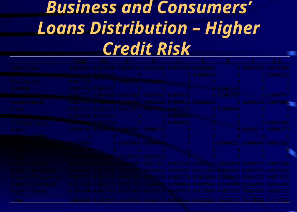
Total 1.0000000 0.1960590 0.2708955 0.1025478 0.0878516 0.0839215 0.0120733 0.0721901 0.1744612

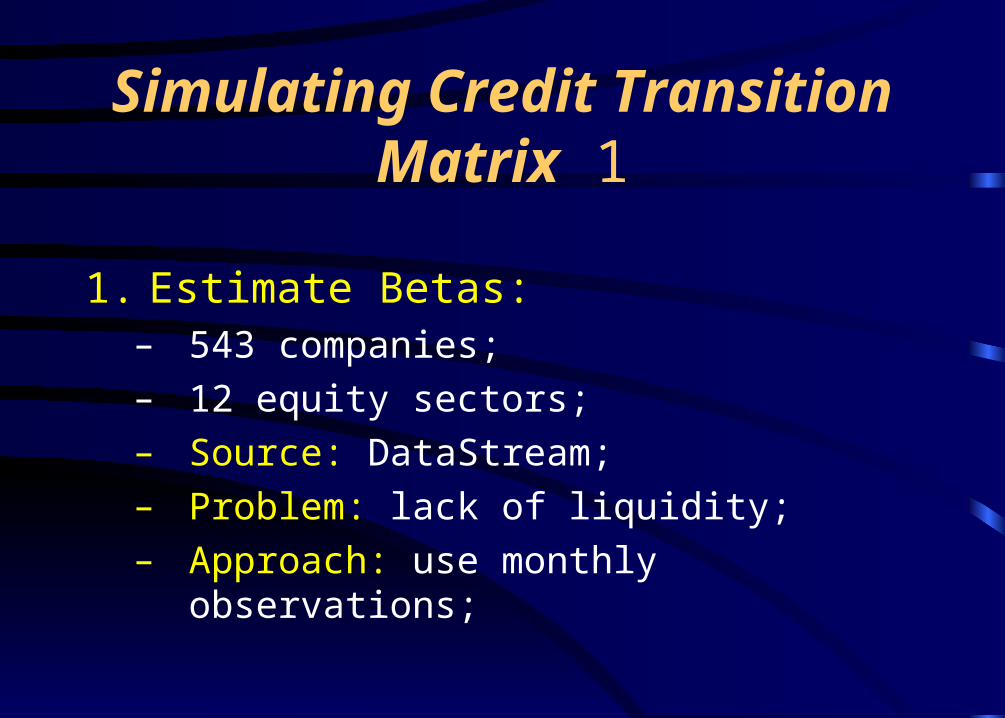
Simulating Credit Transition Matrix 1

1. Estimate Betas:– 543 companies;– 12 equity sectors;– Source: DataStream;– Problem: lack of liquidity;– Approach: use monthly observations;

Simulating Credit Transition Matrix 2

2. Distribute debt-to-value ratios by credit risk category:

– Data source: DataStream.– Credit risk category: weighted average of those

assigned by banks in Brazil.– Distributional Analysis: Analyze the distribution

of company debt-to-value ratios for various credit risk categories.

Simulating Credit Transition Matrix 3

• More on debt-to-value ratios:– Target: the firms’ current and planned future debt-to-value

ratio.– The upper and lower bounds represent the values of debt

ratios at which a company would move to a higher/lower credit rating .

– Example (companies in the B credit level): if the simulated debt ratios increase to more than 0.90 then they would fall to credit rating C.

– Conclusion: credit risk rating deteriorates as systematic and unsystematic components of risk increase, and as debt-to-value ratio increases

AA A B C D E F G + H Debt Ratios Lower bound - 0.51 0.67 0.78 0.79 0.80 0.85 0.96 Target 0.38 0.61 0.82 0.84 0.88 0.89 0.89 0.96 Upper bound 0.53 0.78 0.90 0.92 0.93 0.93 0.95 0.96 Beta 0.67 0.85 1.00 1.10 1.20 1.30 1.36 - Firm-specific risk 0.38 0.55 0.69 0.71 0.77 0.78 0.72 -

Simulating Credit Transition Matrix 4

3. Final step:– For each simulation run, estimate returns on market

index (assumed to follow a GBM) and on companies, via CAPM.

– Use returns to estimate a distribution of possible future equity market values and debt ratios.

– The simulated debt ratios are then mapped into the credit ratings as in the previous table.

–

Panel A: Estimated Transition Matrix, for Brazilian companies, using the PSA approach.

AA A B C D E F G+H AA 90.35% 9.65% 0.00% 0.00% 0.00% 0.00% 0.00% 0.00% A 11.40% 79.63% 8.93% 0.05% 0.00% 0.00% 0.00% 0.00% B 0.40% 4.95% 75.33% 10.00% 3.10% 1.55% 3.45% 1.23% C 0.15% 2.70% 12.60% 68.63% 4.88% 2.23% 5.48% 3.35% D 0.03% 0.70% 4.45% 1.48% 61.48% 4.88% 8.85% 18.15% E 0.00% 0.58% 3.78% 1.25% 0.85% 56.18% 10.48% 26.90% F 0.00% 0.23% 2.33% 1.23% 0.75% 7.30% 60.38% 27.80%

Panel B: Brazilian Credit Risk Bureau’s Transition Matrix (adjusted for repayments, for two large Brazilian banks, and weighted averaged between the periods of June 2000 to June 2001, and June 2001 to June 2002).

AA A B C D E F G+H AA 90.08% 6.43% 2.05% 0.53% 0.18% 0.03% 0.03% 0.68% A 11.90% 69.03% 10.15% 4.73% 2.13% 0.30% 0.43% 1.40% B 3.28% 11.03% 71.88% 9.23% 2.00% 0.48% 0.55% 1.63% C 3.28% 4.18% 15.25% 67.35% 4.65% 0.90% 1.33% 3.08% D 1.08% 1.85% 4.00% 5.13% 60.20% 3.90% 5.43% 18.43% E 0.13% 7.75% 0.53% 0.83% 4.05% 55.80% 4.03% 26.83% F 0.78% 0.60% 1.15% 2.25% 3.10% 7.60% 56.80% 27.63%

Panel C: Difference between simulated and historical transition matrices.

AA A B C D E F G+H AA 0.27% 3.23% -2.05% -0.53% -0.18% -0.03% -0.03% -0.68% A -0.50% 10.60% -1.23% -4.68% -2.13% -0.30% -0.43% -1.40% B -2.88% -6.08% 3.45% 0.78% 1.10% 1.08% 2.90% -0.40% C -3.13% -1.48% -2.65% 1.28% 0.23% 1.33% 4.15% 0.28% D -1.05% -1.15% 0.45% -3.65% 1.28% 0.98% 3.43% -0.28% E -0.13% -7.18% 3.25% 0.43% -3.20% 0.37% 6.45% 0.08% F -0.78% -0.38% 1.18% -1.03% -2.35% -0.30% 3.58% 0.18%

Descriptive Statistics

Mean 0.00002

25th percentile -0.01169

50th percentile -0.00150

75th percentile 0.01081

Maximum 0.10600

Minimum -0.07175

Single Bank Risk Analysis (12/31/2002)

Simulated Capital Ratios: (Assets-Liab)/Assets

Bank NumberInterest Rate Environment

Initial Capital Ratio (Assets-Liab) /Assets Mean Std. DeviationMaximum Minimum 95% 99% Notes

1 Current 0.141080092 0.459732 0.029262 0.526489 0.329407 0.402689 0.368644

Lower 0.141080092 0.333984 0.040558 0.414077 0.149469 0.259208 0.2052

Conc on Highly rated consumer loans

8 Current 0.05076476 0.085325 0.023479 0.141615 0.000477 0.043254 0.017243 Gov. loans .26,Lower 0.05076476 0.04537 0.020547 0.106784 -0.041866 0.008859 -0.010365 Bus .24

Cons. .12

9 Current 0.007268001 0.127821 0.022378 0.196526 0.047793 0.089778 0.067242 Gov. loans .06,Lower 0.007268001 0.05822 0.019731 0.136709 -0.005396 0.007401 0.024984 Bus .32

Cons. .12

10 Current -0.065937796 0.07902 0.007798 0.100615 0.043576 0.065007 0.055333 Gov. loans .4,Lower -0.065937796 0.002516 0.007798 0.017282 -0.015739 -0.008813 -0.015215 Bus .15

Cons. .14

Banking System Systemic Risk Analysis

Systemic risk vs. lower interest rate spread:– Three banks operating simultaneously in the

same macroeconomic/financial environment.– Same asset liability structure (with ‘risk-free’

loans).– Same credit risk exposure (high).– Different inter-bank exposure.– Initial capital level = 15%

Simulation Results 9

• Systemic risk vs. lower interest rate spread (cont.):– Results:

• Probability of a systemic depletion of capital increases substantially.

• Inter-bank exposures becomes an issue (the role of a cascade failure).

Panel A: Target Capital Ratio = 0.01

Simulated Probabilities At least one bank < target1 All three banks < target2

Inter-bank Exposure

lower interest rates

higher interest rates

lower interest rates

higher interest rates

0.00 1.95% 0.65% 0.15% 0.15% 0.01 1.95% 0.65% 0.65% 0.25% 0.03 1.95% 0.65% 0.90% 0.35% 0.05 1.95% 0.65% 1.35% 0.40% 0.07 1.95% 0.65% 1.75% 0.50% 0.09 1.95% 0.65% 1.90% 0.60% 0.10 1.95% 0.65% 1.95% 0.65%

Panel B: Target Capital Ratio = 0.05

Simulated Probabilities At least one bank < target1 All three banks < target2

Inter-bank Exposure

lower interest rates

higher interest rates

lower interest rates

higher interest rates

0.00 6.50% 1.55% 1.25% 0.35% 0.01 6.50% 1.55% 1.95% 0.60% 0.03 6.50% 1.55% 3.35% 1.05% 0.05 6.50% 1.55% 4.40% 1.25% 0.07 6.50% 1.55% 5.25% 1.45% 0.09 6.50% 1.55% 5.90% 1.50% 0.10 6.50% 1.55% 5.95% 1.50%

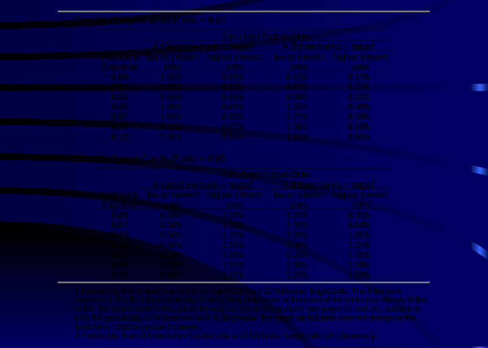
1 Probability that at least one of banks’ capital ratios will fall below target ratio. The inter-bank exposure will affect the probability of defaulting only when at least one of the banks has already fallen below the target capital ratio, given the way we set up this analysis (see pages 23 and 24), and this is why the probability of at least one bank falling below the target capital ratio does not change as the inter-bank credit exposure increases. 2 Probability that all three banks’capital ratio will fall below target ratio simultaneously.

Extensions

• It is quite possible to extend this analysis in at least five directions: – model more than three banks simultaneously;– model stochastic updates for volatilities and

correlations;– develop a methodology for explicitly modeling the

credit risk of consumers loans;– model the risk of a correlated government default

and its impact on banks; and– model correlated derivative security risk exposure.

Conclusions 1• Our preliminary simulations indicated that the risk of

the hypothetical banks studied failing is small, as is the level of systemic bank risk. Further systemic bank risk is not very sensitive to the level of inter-bank credit exposures and to the credit risk profile of loans held by banks. There are at least three potential explanations for this result: (i) the large amount of ‘risk-free’ loans held by banks; (ii) the high capital ratios with which the hypothetical banks operate; and (iii) the large interest rate spreads earned by banks, which are much larger than the default rates on business and consumer loans.

Conclusions 2

• We found the large interest rate spreads to be the most important element on our analysis. When we analyze hypothetical banks earning much more modest (but perhaps typical) interest rate spreads, bank failure risk and systemic bank risk increase substantially. Under this circumstance both inter-bank credit exposure as well as the credit quality of bank loan portfolios become important risk factors.

Conclusions 3

All the conclusions are our own, and do not represent the views of

Banco Central do Brasil