Modeling Basics: 4. Numerical ODE SolvingIn Excel5. Solving ODEs in Mathematica

By Peter WoolfUniversity of Michigan

Michigan Chemical Process Dynamics and Controls Open Textbook

version 1.0

Creative commons

Case study: water storage

Water is vitally important for industry, agriculture, domestic consumption.

Industrial use

Domestic use

Agriculturaluse29.1x1010 m3

3.6x1010 m3

12.1x1010 m3

Data from http://www.newton.dep.anl.gov/askasci/gen01/gen01629.htm

Industrial use

Domestic use

Agriculturaluse29.1x1010 m3

3.6x1010 m3

12.1x1010 m3

Data from http://www.newton.dep.anl.gov/askasci/gen01/gen01629.htm

Industrial use

Domestic use

Agriculturaluse29.1x1010 m3

3.6x1010 m3

12.1x1010 m3

Data from http://www.newton.dep.anl.gov/askasci/gen01/gen01629.htm

Key Question: Have you stored enough water?

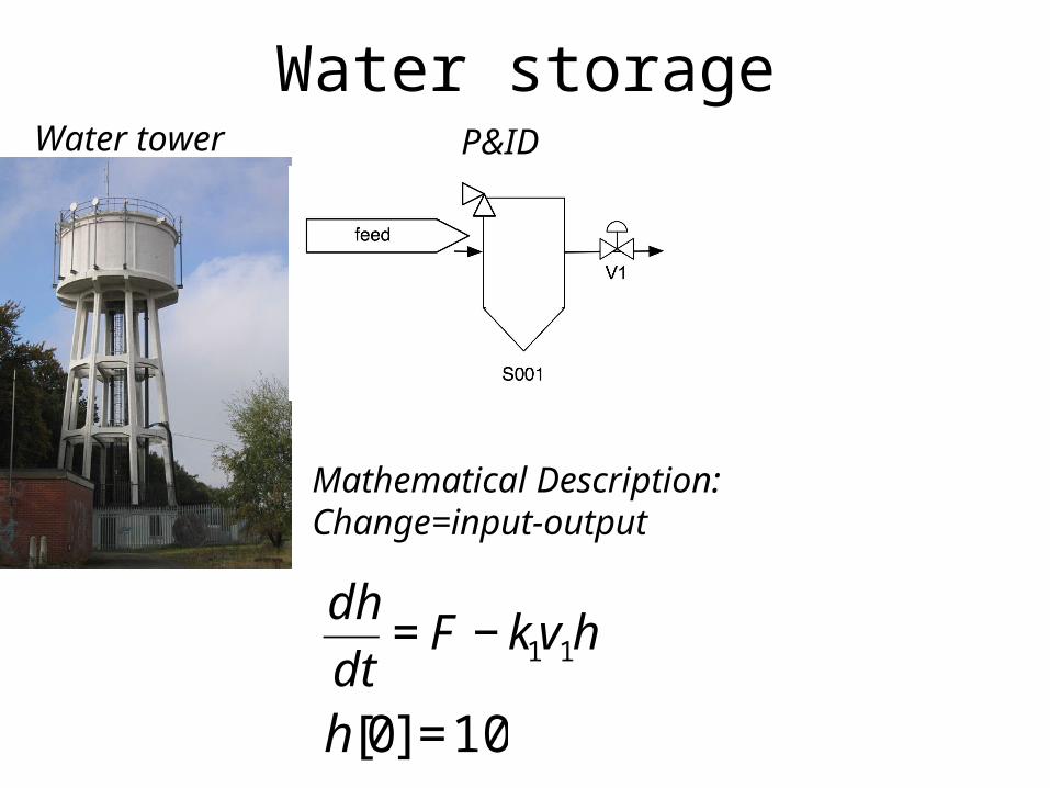
Water storageWater tower P&ID

Mathematical Description:Change=input-output

€

dh

dt= F − k1v1h

€

h[0] =10

€

dh

dt= F − k1v1h

€

h[0] =10

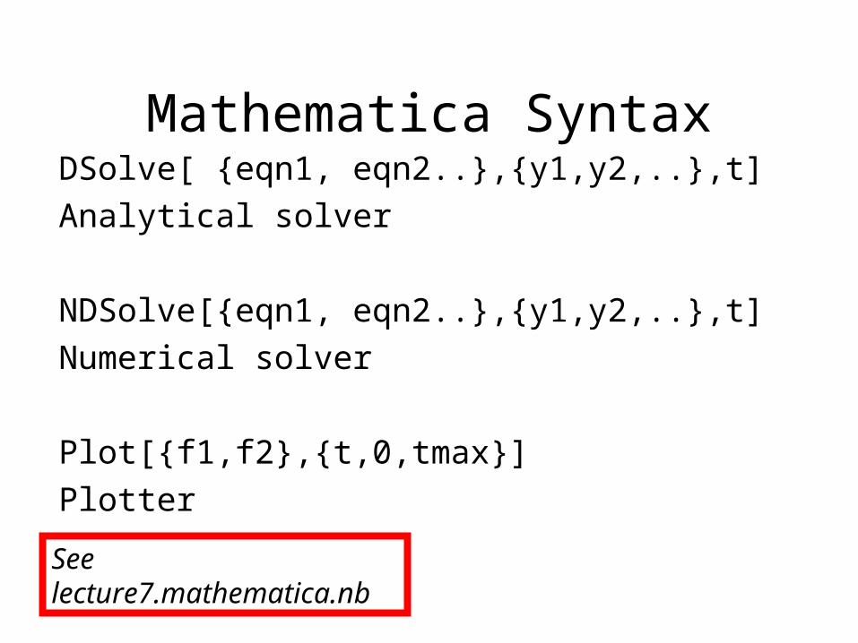
How to solve this set of equations?

• Hand calculation• Software calculation using Mathematica for example• Often not possible for “real” systems• Even if possible, sometimes not useful

• Integrate with software such as Excel or Mathematica (or many others)• Integration can be tricky• Need to know all parameters• Can be computationally demanding

Analytical solutionNumerical solution

Mathematica SyntaxDSolve[ {eqn1, eqn2..},{y1,y2,..},t]

Analytical solver

NDSolve[{eqn1, eqn2..},{y1,y2,..},t]

Numerical solver

Plot[{f1,f2},{t,0,tmax}]

Plotter

See lecture7.mathematica.nb

What if your feed varies in a non-functional way?

Time (hours)

feed

0 1.0

0.5 1.1

1 1.3

1.5 1.4

2 1.2

2.5 0.9

3 0.8

3.5 1.1

Numerical integration!

Numerical ODE solving

time0 0.1

Time step=0.1

Tank depth(h)

True solution

€

dh

dt= F − k1v1h

€

h[0] =10

10

Slope: F-k1v1(10)

€

dh

dt≈

Δh

Δt=hi+1 − hi

Δt= F − k1v1h

€

hi+1 = hi + Δt F − k1v1h[ ]

Euler’s method!

Numerical approx

Numerical ODE solving

time0 0.1

Time step=0.1

Tank depth(h)

10

Slope: F-k1v1(10)

Notes on Euler’s method:• Perfect fit for linear systems• Works well for nonlinear systems if the time step is small (everything is locally linear)• If time step is too large can explode• Small time steps mean slow calculations

Numerical ODE solving

time0 0.1

Time step=0.1

Tank depth(h)

10

Notes on Euler’s method:• Perfect fit for linear systems• Works well for nonlinear systems if the time step is small (everything is locally linear)• If time step is too large can explode• Small time steps mean slow calculations

6.0x103023

Numerical error!

Time step=0.01

Numerical ODE solving

time0 0.1

Time step=0.1

Tank depth(h)

10

Is there a way we could use a larger time step but retain accuracy?

€

hi+1 = hi + Δt slopes [ ]

Solution: take some sort of weighted average of slopes at intermediate points to estimate the next value.

Runge-Kutta methods!

Numerical ODE solving

time0 0.1

Time step=0.1

Tank depth(h)

10

€

hi+1 = hi + Δt slopes [ ]

4th order Runge-Kutta

€

slopes =1

6k1 + 2k2 + 2k3 + k4[ ]

Where

€

k2 = f (0 + Δt /2,ho + k1Δt /2)

€

k3 = f (0 + Δt /2,ho + k2Δt /2)

€

k4 = f (0 + Δt,ho + k3Δt)€

k1 = f (0,ho) Euler’s method

Numerical ODE solving

time0 0.1

Time step=0.1

Tank depth(h)

10

€

hi+1 = hi + Δt slopes [ ]Why stop at 4th order? 5th order is similar but with different weightings

Upsides:1) Larger step sizes possible2) Can be more stable3) Often more

computationally efficientDownsides:1) Complex to implement2) Similar accuracy can often

be achieved using Euler’s method which is easy to implement

Industrial use

Domestic use

Agriculturaluse29.1x1010 m3

3.6x1010 m3

12.1x1010 m3

Data from http://www.newton.dep.anl.gov/askasci/gen01/gen01629.htm

Key Question: Have you stored enough water?

See lecture7.excel.xls

Take home messages

• Numerical simulation of differential equations can help you model very complex systems

• Sometimes slower, simpler method are better as your time is often more valuable than a computers

• Analytical results can be helpful in restricted cases.. Use Mathematica to handle the algebra