Modeling Beacon Period Length of the UWB and 60-GHz mmWave WPANs Based on ECMA-368 and ECMA-387 Standards Hossein Ajorloo and Mohammad Taghi Manzuri-Shalmani Abstract—To evaluate the performance of the distributed medium access control layer of the emerging ultrawideband and 60-GHz millimeter wave (mmWave) wireless personal area networks based on ECMA-368 and ECMA-387 standards, the first step is to determine the beacon period length (BPL) of the superframe in a given network. In this paper, we provide an analytical model for the probability mass function (PMF) of the BPL as a function of the network dimensions, number of beaconing devices, antenna beamwidth, and the transmission range of the devices. To enable devices with steerable directional antennas in the ECMA-387 standard to have simultaneous communications with neighbors in their different antenna sectors, we propose an improvement to the standard for which we computed the PMF of the BPL in its worst case. The effect of beacon period (BP) contraction on the PMF is also considered and modeled. The proposed model for all cases is evaluated by simulating different scenarios in the network and the results show that on average, the model for the average BPL has an error of 1.2 and 2.5 percent in the current definition of the standard and in the proposed modification, respectively, without BP contraction and 0.9 and 1.5 percent, respectively, with BP contraction. Index Terms—Beacon period length, medium access control, ultrawideband, 60-GHz mmWave, wireless personal area network Ç 1 INTRODUCTION M ODELING the medium access control (MAC) layer for emerging wireless technologies can help the standard bodies to resolve shortcomings in their standards and also can provide a good perspective for manufacturers to predict problems associated to any policy defined in the MAC layer, and in some cases can prevent the failure of a standard in global acceptance by the industry. Wireless personal area networks (WPANs) are known as the short- range wireless communication systems providing peer-to- peer connectivity between wireless devices. Two technolo- gies will play the major role in the future high-speed WPANs [1]: UWB and 60-GHz mmWave. UWB is defined at 3.1-10.6 GHz band and can provide data rates of up to 480 Mbps. This band is used by other technologies and hence, a rigorous restriction is applied by the Federal Communications Commission (FCC) to the power level of compliant devices. The 60-GHz technology, on the other hand, is defined in a 9 GHz unlicensed band around the 60 GHz frequency and can provide data rates of more than 2 Gbps. After the failure of the IEEE 802.15.3a in providing a standard for the UWB WPAN, the multiband orthogonal frequency division multiplexing UWB (MB- OFDM UWB) is promoted by the ECMA-368 standard [2] which unlike the IEEE 802.15.3a defines an unstructured communication mechanism. This distributed architecture led to the success and global acceptance of this standard for the UWB WPAN [3]. Because of the high propagation loss at the 60 GHz frequency, the devices should use steerable antenna arrays to provide high data rates and/or successful communica- tion up to 10 meters. The antenna array can be fabricated at the chip level thanks to the very short wavelength of this frequency (about 5 mm). Recent advances in the radio frequency circuitry resulted in the successful on-chip CMOS front-ends at the 60 GHz frequency [4], [5], [6], [7]. For example, a complete 60 GHz communication system is reported in [7] which provides 4 Gbps data rate using on-chip steerable antenna arrays with beam steering latency of less than 1 ms. Three standards are defined for the 60 GHz WPANs, namely, WirelessHD [8], IEEE 802.15.3c [9], and ECMA-387 [10]. While the first two standards define centralized MAC architectures, the last one defines an unstructured MAC mechanism similar to ECMA-368. Because of this distributed architecture, it seems in the future, the ECMA-387 standard will occupy a considerable portion of the 60 GHz WPANs’ market share, similar to UWB technology. There exist lots of valuable works reported in the literature trying to model the policies defined in the MAC layer of these technologies. While most of them provide an analytical model for the throughput and delay criterions [11], [12], [13], [14], [15], [16], [17], [18], [19], a few works are available in the literature about the beaconing mechanism of the ECMA-368 and ECMA-387 standards. For some in- stances, the problem of beacon collision at the association stage of the ECMA-368 is studied by Vishnevsky et al. [3] and an analytical model for the evaluation of the perfor- mance of different slot selection methods is presented. Some works also devoted to the definition of optimum beacon transmission for the IEEE 802.15.3c standard to reduce the communication overhead imposed by the redundant bea- cons [20], [21]. IEEE TRANSACTIONS ON MOBILE COMPUTING, VOL. 12, NO. 6, JUNE 2013 1201 . The authors are with the Department of Computer Engineering, Sharif University of Technology, Azadi Ave., Tehran, Iran. E-mail: [email protected], [email protected]. Manuscript received 30 July 2011; revised 10 Dec. 2011; accepted 29 Mar. 2012; published online 5 Apr. 2012. For information on obtaining reprints of this article, please send e-mail to: [email protected], and reference IEEECS Log Number TMC-2011-07-0428. Digital Object Identifier no. 10.1109/TMC.2012.91. 1536-1233/13/$31.00 ß 2013 IEEE Published by the IEEE CS, CASS, ComSoc, IES, & SPS
Transcript
Modeling Beacon Period Length of the UWBand 60-GHz mmWave WPANs Based on
ECMA-368 and ECMA-387 StandardsHossein Ajorloo and Mohammad Taghi Manzuri-Shalmani
Abstract—To evaluate the performance of the distributed medium access control layer of the emerging ultrawideband and 60-GHz
millimeter wave (mmWave) wireless personal area networks based on ECMA-368 and ECMA-387 standards, the first step is to
determine the beacon period length (BPL) of the superframe in a given network. In this paper, we provide an analytical model for the
probability mass function (PMF) of the BPL as a function of the network dimensions, number of beaconing devices, antenna
beamwidth, and the transmission range of the devices. To enable devices with steerable directional antennas in the ECMA-387
standard to have simultaneous communications with neighbors in their different antenna sectors, we propose an improvement to the
standard for which we computed the PMF of the BPL in its worst case. The effect of beacon period (BP) contraction on the PMF is also
considered and modeled. The proposed model for all cases is evaluated by simulating different scenarios in the network and the
results show that on average, the model for the average BPL has an error of 1.2 and 2.5 percent in the current definition of the standard
and in the proposed modification, respectively, without BP contraction and 0.9 and 1.5 percent, respectively, with BP contraction.
Index Terms—Beacon period length, medium access control, ultrawideband, 60-GHz mmWave, wireless personal area network
Ç
1 INTRODUCTION
MODELING the medium access control (MAC) layer foremerging wireless technologies can help the standard
bodies to resolve shortcomings in their standards and alsocan provide a good perspective for manufacturers topredict problems associated to any policy defined in theMAC layer, and in some cases can prevent the failure of astandard in global acceptance by the industry. Wirelesspersonal area networks (WPANs) are known as the short-range wireless communication systems providing peer-to-peer connectivity between wireless devices. Two technolo-gies will play the major role in the future high-speedWPANs [1]: UWB and 60-GHz mmWave.
UWB is defined at 3.1-10.6 GHz band and can providedata rates of up to 480 Mbps. This band is used by othertechnologies and hence, a rigorous restriction is applied bythe Federal Communications Commission (FCC) to thepower level of compliant devices. The 60-GHz technology,on the other hand, is defined in a 9 GHz unlicensed bandaround the 60 GHz frequency and can provide data rates ofmore than 2 Gbps. After the failure of the IEEE 802.15.3a inproviding a standard for the UWB WPAN, the multibandorthogonal frequency division multiplexing UWB (MB-OFDM UWB) is promoted by the ECMA-368 standard [2]which unlike the IEEE 802.15.3a defines an unstructuredcommunication mechanism. This distributed architectureled to the success and global acceptance of this standard forthe UWB WPAN [3].
Because of the high propagation loss at the 60 GHzfrequency, the devices should use steerable antenna arraysto provide high data rates and/or successful communica-tion up to 10 meters. The antenna array can be fabricatedat the chip level thanks to the very short wavelength of thisfrequency (about 5 mm). Recent advances in the radiofrequency circuitry resulted in the successful on-chipCMOS front-ends at the 60 GHz frequency [4], [5], [6],[7]. For example, a complete 60 GHz communicationsystem is reported in [7] which provides 4 Gbps data rateusing on-chip steerable antenna arrays with beam steeringlatency of less than 1 ms. Three standards are defined forthe 60 GHz WPANs, namely, WirelessHD [8], IEEE802.15.3c [9], and ECMA-387 [10]. While the first twostandards define centralized MAC architectures, the lastone defines an unstructured MAC mechanism similar toECMA-368. Because of this distributed architecture, itseems in the future, the ECMA-387 standard will occupya considerable portion of the 60 GHz WPANs’ marketshare, similar to UWB technology.
There exist lots of valuable works reported in theliterature trying to model the policies defined in the MAClayer of these technologies. While most of them provide ananalytical model for the throughput and delay criterions[11], [12], [13], [14], [15], [16], [17], [18], [19], a few works areavailable in the literature about the beaconing mechanism ofthe ECMA-368 and ECMA-387 standards. For some in-stances, the problem of beacon collision at the associationstage of the ECMA-368 is studied by Vishnevsky et al. [3]and an analytical model for the evaluation of the perfor-mance of different slot selection methods is presented. Someworks also devoted to the definition of optimum beacontransmission for the IEEE 802.15.3c standard to reduce thecommunication overhead imposed by the redundant bea-cons [20], [21].
IEEE TRANSACTIONS ON MOBILE COMPUTING, VOL. 12, NO. 6, JUNE 2013 1201
. The authors are with the Department of Computer Engineering, SharifUniversity of Technology, Azadi Ave., Tehran, Iran.E-mail: [email protected], [email protected].
Manuscript received 30 July 2011; revised 10 Dec. 2011; accepted 29 Mar.2012; published online 5 Apr. 2012.For information on obtaining reprints of this article, please send e-mail to:[email protected], and reference IEEECS Log Number TMC-2011-07-0428.Digital Object Identifier no. 10.1109/TMC.2012.91.
1536-1233/13/$31.00 � 2013 IEEE Published by the IEEE CS, CASS, ComSoc, IES, & SPS
For the synchronization of the devices in an ECMA-368and/or 387 networks, each device (in ECMA-387, devices oftype A/B) transmits its own beacon at the beginning partof the superframe (SF) to provide the required informationfor the synchronization and communication with otherdevices. The remaining slots in the SF are used for datacommunication between devices. Hence, the BPL is variablein a network and each device may sense different number ofdevices around it and so experiences a different value of BPLwith respect to other devices in the same network. Toevaluate the performance of these standards, such asmodeling the throughput, delay, power consumption, andfairness, one should first compute the average BPL of a givennetwork. The lack of such model in the literature motivatedus to theoretically calculate the PMF of the BPL in this paper.
The remainder of this paper is organized as follows: InSection 2, we briefly discuss the beaconing mechanismdefined in the ECMA-368 and 387 standards. Section 3presents the proposed BPL model for the current definitionof the standards. The enhancement to the ECMA-387standard is discussed in Section 4 and the BPL model forthe enhanced version is presented in Section 5. The effectof BP contraction is modeled in Section 6. Correctness ofthe models is evaluated in Section 7. Finally, Section 8concludes the paper.
Notations. The notations of the variables used in thepaper are presented in Table 1. Also, we used capital letterfor the PMFs (P ) and lower case letter for other probabilities(p). Somewhere in the paper, the subscript of P is omittedfor the sake of simplicity.
2 THE BEACONING MECHANISM OF THE ECMA-368AND ECMA-387 STANDARDS
In this section, a brief discussion of the beacon transmissionmechanism of the ECMA-368 and 387 standards is presented.
For the sake of synchronization and data communication,each device (in ECMA-387, each device of type A/B) sendsits own beacon which contains required information forcommunication with other devices in its vicinity. The devicesalign their SFs with the slowest device in the network.
After powering up, a device shall first discover anotherdevice with which it intends to communicate. This is donein a particular channel using a device discovery mechanismbased on the device’s type using robust modulation andcoding schemes in omnidirectional antenna mode. Devicesof type A execute an antenna training mechanism followingthe device discovery.
Each device provides a beacon map (B-map) in whichslots adopted by the neighbor devices are indicated. Fig. 1shows an example of such a B-map sustained by a devicein the network. A device is considered as neighbor by anyother device, if its beacon can be received directly. Adevice will consider any slot as unavailable if it is used byany of its neighbors or by their neighbors. A device shalltransmit a beacon in a beacon slot chosen from up tomBPExtension beacon slots located after the highestnumbered unavailable beacon slot it observed in the lastSF and within mMaxBPLength after the beacon period start
1202 IEEE TRANSACTIONS ON MOBILE COMPUTING, VOL. 12, NO. 6, JUNE 2013
TABLE 1The Notations of Variables and Parameters in the Paper
Fig. 1. An example of the beacon map provided by a device in thenetwork (from [2] and [10]).
time. By this policy, a device will not transmit its beacon inthe slots in which its neighbors are sending their beaconsor listening to their neighbors’ beacon, and hence, thebeacon collision will be avoided.
All devices of ECMA-368 and type B devices of ECMA-387 use omnidirectional antennas. On the other hand, type Adevices in ECMA-387 shall use steerable directional anten-nas and send their beacon in the direction of their recipient.
The beacon period length is variable depending on thenumber of neighbors of the devices. The maximum BPL canreach the mMaxBPLength defined in the standard. The BPLis defined as the maximum unavailable slot index seen byany device. The remaining slots, named data period, areused for data communication between devices. Fig. 2 showsa sample network containing 30 devices with omni (Fig. 2a)and steerable directional antennas (Figs. 2b and 2c) withbeamwidth �=6. Each circle indicates a device, and eachdotted line indicates the neighborhood relation betweentwo devices. The vertical axis shows the BPL values for eachdevice which is indicated by a vertical bar on its circle.In Fig. 2b, we assume that each device sends just one beaconin each SF, but in Fig. 2c we assume that a device sends onebeacon per each antenna sector on which it has at least oneneighbor. The last case is not defined in the standard, butwe propose it in Section 4.
To reduce the BPL and to let the devices to use more slotsfor data communication and prevent the waste of the slots,a BP contraction mechanism is defined in the standards. Adevice shall consider its beacon to be movable if in theprevious SF it found at least one available beacon slotbetween the signaling slots and the beacon slot it indicatesin its beacon in the current SF. A device not involved in abeacon slot collision or a BP merge shall shift its beacon intothe earliest available beacon slot following the signalingbeacon slots in the BP of the next SF.
3 THE PROPOSED MODEL FOR THE PMF OF
THE BPL IN THE CURRENT DEFINITION OF
THE STANDARDS WITHOUT BP CONTRACTION
In this section, we develop an analytical model forcomputation of the PMF of the BPL values. A brief discussion
on the beacon transmission mechanism of the ECMA-368
and 387 standards is given in Section 2. We begin our analysis
by the following assumptions:
. N devices are scattered randomly in the unit squarewith uniform distribution.
. The transmission range (Tx range) and 3 dB antennaarray beamwidth for all devices equal r and �3dB,respectively.
. Each device only sends and receives beacons in its�3dB beam.
. None of the devices miss the beacon of otherdevices more than mMaxLostBeacons consecutiveSFs and so they sustain their connectivity with otherneighbors.
. We consider the network is in the steady-statecondition, i.e., all devices which sense each other,align their SFs and they can retrain their antennasbefore mMaxLostBeacons in small movements andchannel changes, so the network is considered asstable. Moreover, the movements are consideredsmall enough such that the devices do not exit fromeach others’ neighborhood.
Note that with �3dB ¼ 2� the problem reduces to the
omnidirectional case. In this section, we ignore BP contrac-
tion. We shall deal with it in Section 6.We are now going to develop our model for the PMF of
the BPL. Each device computes its BPL as the index of the
highest unavailable beacon slot number, therefore
PBðB ¼ kjN2Þ ¼�1� paðskjN2Þ
� YMj¼kþ1
paðsjjN2Þ; ð1Þ
in which sk denotes the kth slot, and paðskjN2Þ is the
probability of availability of the slot sk, givenN2 “second order
neighbors” (SON). The concept of SON introduced in this
paper means a device which is whether the neighbor or the
neighbor of a neighbor of a given device. Equation (1) holds
since a device announces the maximum index of unavailable
slots in its B-map to be k if slot sk is unavailable and the
remaining M � k slots are available. M ¼ mMaxBPLength
is the maximum allowable BPL (Fig. 1).
AJORLOO AND MANZURI-SHALMANI: MODELING BEACON PERIOD LENGTH OF THE UWB AND 60-GHZ MMWAVE WPANS BASED ON... 1203
Fig. 2. Sample network containing 30 nodes with (a) omni, and (b), (c) steerable antennas with beamwidth �=6, and Tx range of 0.25 normalized tonetwork dimensions. In (b), each device sends just one beacon in the direction of its peer, but in (c) each device sends in all antenna sectors onwhich it has a neighbor. The BPL values are indicated by a vertical bar on each node. The BP contraction is disabled.
A device considers a given slot as available if it ischosen neither by itself nor by none of its SONs for theirbeaconing. Consequently,
paðskjN2Þ ¼�1� pcðskjN2Þ
�N2þ1; ð2Þ
where pcðskjN2Þ denotes the probability that a device withN2 SONs chooses slot sk for its beacon transmission. In (2),we assumed that the probabilities 1� pcðskjN2Þ are inde-pendent. This is not true in all scenarios. In particular, whenN and r take large values, this assumption is no longervalid. However, as we have shown in Section 7, thisequation produces satisfactory results for most scenariosand in typical networks, it leads to acceptable error.
To compute pc, we start by the following conditionalprobability:
pcðskjD ¼ d; U ¼ u;N2Þ
¼
1; d ¼ 1; k ¼ 1
0; d ¼ 1; k > 1
0; d > 1; k ¼ 1
0; d ¼ 2; k > minðmþ 1;MÞ1
minðm;MÞ ; d ¼ 2; 2 � k � minðmþ1;MÞp1
minðuþm;MÞ � dþ 1; d > 2; 1 � k � u
1
minðuþm;MÞ � dþ 1; d > 2; uþ 1 � k
� minðuþm;MÞ0; o:w:;
8>>>>>>>>>>>>>>>>>>>>><>>>>>>>>>>>>>>>>>>>>>:
ð3Þ
in which, m ¼ mBPExtension and
p1 ¼Xd�1
�¼2
�pcðsujD ¼ �;N2Þ
Yd�1
�¼2�6¼�
�1� pcðskjD ¼ �; N2Þ
��: ð4Þ
In (3), pcðskjD ¼ d; U ¼ u;N2Þ denotes the conditionalprobability of choosing slot sk given that the device has N2
SONs and it is the dth device between its SONs that ispowered on and the maximum unavailable slot seen by thisdevice is u. An explanation on (3) is given in Appendix A,which can be found on the Computer Society DigitalLibrary at http://doi.ieeecomputersociety.org/10.1109/TMC.2012.91. As we mentioned in Appendix A, availablein the online supplemental material, this is an approxima-tion on pc. In Appendix B, available in the onlinesupplemental material, the method to obtain the exactvalue for pc is presented which is computationally toocomplex. To compute (3), we need the conditional prob-ability pcðskjD ¼ d;N2Þ which can be obtained using thetotal probability theorem as follows:
pcðskjD ¼ d;N2Þ
¼XMu¼1
pcðskjD ¼ d; U ¼ u;N2ÞpUðU ¼ ujD ¼ d;N2Þ:ð5Þ
Again, the first four conditions of (3) exist for pcðskjD ¼d;N2Þ which are omitted in (5) for the sake of simplicity. In
(5), we need pUðU ¼ ujD ¼ d;N2Þ, the probability that themaximum unavailable slot seen by a device is u given that ithas N2 SONs and it is the dth device which is powered on.This probability can be computed as follows:
pUðU ¼ ujD ¼ d;N2Þ
¼
0; d ¼ 1
1; d ¼ 2; u ¼ 1
0; d ¼ 2; u > 1
0; d > 2; u < d� 1
0; d > 2; u > min�ðd� 2Þmþ 1;M
�p2; o:w:;
8>>>>>>>><>>>>>>>>:
ð6Þ
in which
p2 ¼Xd�1
�¼2
�pcðsujD ¼ �;N2Þ
Yd�1
�¼2�6¼�
YMj¼uþ1
ð1� pcðsjjD ¼ �; N2ÞÞ�:
ð7Þ
An explanation of (6) is given in Appendix C, availablein the online supplemental material.
Note that we arrived at a set of recursive formulas for thecomputation of pcðskjD ¼ d;N2Þ. More precisely, (3)-(7)compute pc for D ¼ d based on pc for D ¼ 2 . . . d� 1. InAppendix D, available in the online supplemental material,an algorithm for computation of pcðskjD ¼ d;N2Þ is given.Using the total probability theorem, we compute pcðskjN2Þas follows:
pcðskjN2Þ ¼XN2þ1
d¼1
pcðskjD ¼ d;N2ÞP ðD ¼ djN2Þ: ð8Þ
In (8), the summation is taken from 1 up to N2 þ 1, becausethe device has N2 SONs, and hence it can be the first-(N2 þ 1)st device between its SONs considering itself whichis powered on. Since, there exists no preference between thedevices, P ðD ¼ djN2Þ follows the uniform distribution asfollows:
P ðD ¼ djN2Þ ¼1
N2 þ 1: ð9Þ
Now, PBðBÞ, the PMF of the BPL can be computed usingthe total probability theorem as follows:
PBðB ¼ kÞ ¼XN�1
N2¼1
PBðB ¼ kjN2ÞP ðN2Þ; ð10Þ
where P ðN2Þ denotes the PMF of the number of the SON.So, we need P ðN2Þ. To compute it, we start by a
conditional probability as follows: for a device to have n2
SONs given that it has n1 first order neighbors (FON) wheren1 � n2, n2 � n1 devices should be the neighbor of at leastone of the n1 neighbors of the considered device, i.e., theylie in its antenna sector range and steer their antenna to thedirection of the neighbor device to choose it as itscommunication peer. N � 1� n2 þ n1 remaining devicesshould be the neighbor of none of the n1 neighbor devices.Therefore, assuming independence between these probabil-ities we arrive at
1204 IEEE TRANSACTIONS ON MOBILE COMPUTING, VOL. 12, NO. 6, JUNE 2013
P ðN2 ¼ n2jN1 ¼ n1Þ
¼N � 1
n2 � n1
� �qn2�n1s 1� qsð ÞN�1�n2þn1 :
ð11Þ
This is a binomial distribution with parametersN � 1 andqs ¼ ð1� ð1� qnÞn1Þð1� qo � qnÞ. qn denotes the probabilitythat a device lies in the antenna sector range of anotherdevice and steers its antenna to the direction of that device tochoose it as its communication peer. This probability can becomputed as follows:
qn ¼qd
N1;avgþ qd
�3dB
2�1� qd
N1;avg
� �; ð12Þ
where qd is the probability that a device lies in the antennasector range of another device. An explanation on (12) isgiven in Appendix E, available in the online supplementalmaterial.
In (12), N1;avg is the average number of FONs of a device,which follows binomial distribution with parameters N � 1and qd, i.e.,
N1;avg ¼XN�1
n¼0
nN � 1n
� �qnd ð1� qdÞ
N�1�n: ð13Þ
When a device powers on, it steers its antenna to thedirection of one of its neighbors around it. This is analogousto consider it as an omnineighbor (the one which lies in thecircle with radius r centered on the device). Hence, if adevice has n1 FONs, one of them is an omnineighbor and theother n1 � 1 neighbors lie in the antenna sector range of thedevice and choose it as their communication peer. Hence,
P ðN1 ¼ n1Þ ¼ðN � 1Þ!
ðn1 � 1Þ!ðN � n1Þ!qoq
n1�1n ; ð14Þ
where qo denotes the probability that a device lies in circlewith radius r around another device. Again, we usedthe approximation that the probabilities that the devices inthe network become the neighbors of a given or a set ofgiven devices are independent.
The PMF of the number of SONs can be computed usingthe total probability theorem as follows:
P ðN2 ¼ n2Þ ¼Xn2
n1¼1
P ðN2 ¼ n2jN1 ¼ n1ÞP ðN1 ¼ n1Þ: ð15Þ
In (12) and (13), qd is the probability that an active device(a device that has a peer) lies in the 3-dB beamwidth and Txrange of a given device and equals
qd ¼�3dB
2�ptqo ð16Þ
in which pt denotes the probability that a given device findsa peer. This probability is defined because a device may notfind any peer. Such devices do not transmit any beacon andhence they do not contribute in the computation of BPL. Adevice (say �) will be able to find a peer if at least one nodelies in its range r and if one of them (say �) is not able tofind a peer, � asks � for antenna training process and theysteer their antenna beams toward direction of each otherand start beaconing. Otherwise, if all of them are active and
transmitting beacons, � lies in the 3-dB beamwidth and
range r of at least one of them. So,
pt ¼ EN1
�1� pN1
t
�þ pN1
t 1� 1� �3dB
2�
� �N1
!( ); ð17Þ
in which EN1f:g takes the average of its argument over N1.
By substituting appropriate values in this equation and by
sorting it based on pt, we arrive at the following equation:
XN�1
k¼1
N � 1
k
� �qkoð1� qoÞ
N�1�k 1� �3dB
2�
� �kpkt
þ pt þ ð1� qoÞN�1 � 1 ¼ 0:
ð18Þ
This is an (N � 1)st order polynomial equation based on
pt which can be solved for pt by numerical approaches. Note
that in the case of omnidirectional antennas, i.e., �3dB ¼ 2�,
(18) reduces to
pt ¼ 1� ð1� qoÞN�1; ð19Þ
which means a device can transmit its beacon if at least onenode lies in its r vicinity.
The value of qo can be computed as follows: qo is theprobability that a node lies in a range less than or equal to rof a given node, i.e.,
qo ¼ FRðrÞ ¼ EX;Y fFRðrjX;Y Þg; ð20Þ
where FRðrjX;Y Þ ¼ P ðR � rjX;Y Þ is the probability that a
device lies in the range r of a given node at position ðX;Y Þof the unit square. This CDF is computed in the Appendix F,
available in the online supplemental material, and equals
FRðrÞ ¼
0; r < 01
2r4 � 8
3r3 þ �r2; 0 � r < 1
� 1
2r4 þ 8r2 þ 4
3
ffiffiffiffiffiffiffiffiffiffiffiffiffir2 � 1p
þ�4 sin�1ð1rÞ � �� 2
�r2 þ 1
3 ; 1 � r <ffiffiffi2p
1; r �ffiffiffi2p
:
8>>>>>>><>>>>>>>:
ð21Þ
Fig. 3 compares the empirical CDF of the distances
between 5,000 pairs of nodes with coordinations randomly
AJORLOO AND MANZURI-SHALMANI: MODELING BEACON PERIOD LENGTH OF THE UWB AND 60-GHZ MMWAVE WPANS BASED ON... 1205
Fig. 3. qo ¼ FRðrÞ, the probability that a device lies in the Tx range of agiven device.
generated in the range ½0; 1�2 to the analytical CDF of (21).This figure shows the correctness of the calculations,empirically. Note that we used the following approximationin our model:
EfBðqoÞg � BðEfqogÞ: ð22Þ
More precisely, instead of computing the BPL, B, interms of the coordinations ðX;Y Þ and then taking theaverage over X and Y , we first took the average of qo over Xand Y and then computed B based on the average value ofqo. However, the exact value for EfBðqoÞg equals
EfBðqoÞg ¼ BðEfqogÞ þB00ðEfqogÞ�2
2
þ � � � þBðnÞðEfqogÞ�nn!þ � � �
ð23Þ
in which BðnÞðEfqogÞ ¼ dn
dqnoBðEfqogÞ, �2 denotes the variance
of qo, and �n¼Efðqo�EfqogÞng is the nth central moment of
qo. However, we used only the first term of (23) in (22)
which is an approximation. However, computing the exact
value leads to a set of complicated equations which should
be solved using numerical methods.The average BPL can be computed from
Bavg ¼XMl¼1
lPBðB ¼ lÞ: ð24Þ
4 THE PROPOSED MODIFICATION TO THE
ECMA-387 STANDARD
In this section, we propose a modification to the ECMA-387 standard to enable a type A device to have connectivityin more than one direction with other devices in itsvicinity. However, in the current version of the standard,since a device is permitted to send only one beacon in eachSF, it can just sustain its connectivity with devices locatedin one of its antenna sectors. If a device needs tocommunicate simultaneously with two devices located inits different antenna sectors, it should send beacons in bothdirections. To provide such facility, we propose to allowdevices to send beacon in any antenna sector they need,i.e., a device is allowed to send multiple beacons in a SF.For this purpose, it is just required to sustain a sector map(S-map) along with the B-map, in which a device says ittransmits/receives beacon in a slot on the indicatedantenna sector. Fig. 4 shows an example of a B-map-S-map pair of a given device. In this figure, for example,device 1 (the owner of B-map-S-map) receives beacon fromdevice 3 in slot 1 on its sector 8 and sends its beacon in slot6 on its sector 4 and in slot 9 on its sector 8. Device 1 in thisexample communicates on its sectors 4 and 8.
When a device tries to find a slot for its beacon, itassumes a slot as available if none of its neighbors in thatdirection choose that slot and if none of them directed in adirection that they cannot receive its beacon in that slot.Note that the devices know their neighbors’ antenna sectorindex meaning since they executed antenna trainingprocedure before the data communication by theirneighbors which they need to communicate. For example,in Fig. 4, slot 1 is available for device 6 to send its beacon
in a direction other than the sector on which it receivesdevice 1’s beacon, if all other neighbors of device 6 in thatdirection can receive its beacon.
On the other hand, this method causes the B-map ofdevices to be larger and so, the average BPL enlarges withrespect to the current definition of the standard. The worstcase arises when all devices in the network transmit beaconin all of their active antenna sectors, i.e., all antenna sectorson which they have at least one neighbor.
Note that in the above we assumed that the devices havejust one radio component which is the case for mostcommercial products. However, if a device has two radios,it can steer its both antenna arrays in two differentdirections to send its beacon in both directions and itshould train its both antennas. This slows down the devices’operation and adds to its complexity and price.
5 THE PROPOSED MODEL FOR THE PMF OF
THE BPL IN THE PROPOSED MODIFICATION
TO THE ECMA-387 STANDARD WITHOUT
BP CONTRACTION
In the following, we compute the PMF of the BPL for theworst case in the modified version of the ECMA-387standard. As we discussed earlier, by the proposedmodification to the ECMA-387 standard, each device oftype A can transmit one beacon per each active sector itpossesses. This enables the device to have connectivity withall devices in its vicinity. In this section, we ignore BPcontraction. We shall deal with it in Section 6.
Equations (1) and (2) hold in this case. To compute pc,two more conditions should be considered: number ofactive antenna sectors, Nas, and current active antennasector, S. In this case, pc can be computed as follows:
pcðskjD ¼ d; U ¼ u; S ¼ s;N2;w; NasÞ ¼1; d ¼ 1; k ¼ 1; s ¼ 1
0; d ¼ 1; k > 1; s ¼ 1
0; d > 1; k ¼ 1
0; s > 1; k ¼ 1
0; d ¼ 2; k > minðmþ 1;MÞ; s ¼ 1
0; d ¼ 1; k > minðmþ 1;MÞ; s ¼ 21
minðm;MÞ ; d ¼ 2; 2 � k � minðmþ 1;MÞ; s ¼ 1
1minðm;MÞ ; d ¼ 1; 2 � k � minðmþ 1;MÞ; s ¼ 2
p3
minðuþm;MÞ�dþ1 ; d > 2; 1 � k < u; s ¼ 1p4
minðuþm;MÞ�sþ1 ; d ¼ 1; 1 � k<u; s>2
1minðuþm;MÞ�dþ1 ; d > 2; uþ 1 � k � minðuþm;MÞ;
s ¼ 11
minðuþm;MÞ�sþ1 ; d ¼ 1; uþ 1 � k � minðuþm;MÞ;s > 2
1206 IEEE TRANSACTIONS ON MOBILE COMPUTING, VOL. 12, NO. 6, JUNE 2013
where p3, p4, and p5 are given by
p3 ¼Xd�1
�¼2
�pcðsujD ¼ �;N2;wÞ
Yd�1
�¼2� 6¼�
�1� pcðskjD ¼ �; N2;wÞ
��;
p4 ¼Xs�1
�¼2
"pcðsujD ¼ d; U ¼ u; s ¼ �;N2;w; NasÞ
Ys�1
&¼1& 6¼�
�1� pcðskjD ¼ d; U ¼ u; S ¼ &; N2;w; NasÞ
�#;
p5 ¼Xd�1
�¼1
"pcðsujD ¼ �;N2;wÞ
"Yd�1
�¼1� 6¼�
�1� pcðskjD ¼ �; N2;wÞ
�#
"Ys�1
&¼1
�1� pcðskjD ¼ d; U ¼ u; S ¼ &; N2;w; NasÞ
�##
þXs�1
�¼1
"pcðsujD ¼ d; U ¼ u; s ¼ �;N2;w; NasÞ
"Yd�1
�¼1
�1� pcðskjD ¼ �; N2;wÞ
�#"Ys�1
&¼1& 6¼�
�1� pcðskjD ¼ d; U ¼ u; S ¼ &; N2;w; NasÞ
�##:
ð26Þ
An explanation on (25) is given in Appendix G, available
in the online supplemental material. To compute (25), we
need the conditional probability pcðskjD ¼ d;N2;wÞ. For this
also, we first need to compute pcðskjD ¼ d; S ¼ s;N2;w; NasÞusing the total probability theorem from
pcðskjD ¼ d; S ¼ s;N2;w; NasÞ
¼XMu¼1
½pcðskjD ¼ d; U ¼ u; S ¼ s;N2;w; NasÞ
pUðU ¼ ujD ¼ d; S ¼ s;N2;w; NasÞ�:
ð27Þ
Again, the first eight conditions of (25) exist for pcðskjD ¼d; S ¼ s;N2;w; NasÞ which are omitted in (27) for the sake of
simplicity. In (27), we needpUðU ¼ ujD ¼ d; S ¼ s;N2;w; NasÞ.This probability can be computed as follows:
pUðU ¼ ujD ¼ d; S ¼ s;N2;w; NasÞ
¼
0; d ¼ 1; s ¼ 1
1; d ¼ 2; u ¼ 1; s ¼ 1
1; d ¼ 1; u ¼ 1; s ¼ 2
0; d ¼ 2; u > 1; s ¼ 1
0; d ¼ 1; u > 1; s ¼ 2
0; u < dþ s� 2; ðd > 2 or s > 2Þ0; u > min
�ðdþ s� 3Þmþ 1;M
�; ðd > 2 or s > 2Þ
p6; o:w:;
8>>>>>>>>>>>>><>>>>>>>>>>>>>:
ð28Þ
in which p6 is given by
p6 ¼Xd�1
�¼1
"pcðsujD ¼ �;N2;wÞ
"Yd�1
�¼1�6¼�
YMj¼uþ1
�1� pcðsjjD ¼ �; N2;wÞ
�#
"Ys�1
&¼1
YMj¼uþ1
ð1� pcðsjjD ¼ d; S ¼ &; N2;w; NasÞÞ##
þXs�1
�¼1
"pcðsujD ¼ d; s ¼ �;N2;w; NasÞ
"Yd�1
�¼1
YMj¼uþ1
�1� pcðsjjD ¼ �; N2;wÞ
�#"Ys�1
&¼1& 6¼�
YMj¼uþ1
�1� pcðsjjD ¼ d; S ¼ &; N2;w; NasÞ
�##:
ð29Þ
An explanation on (28) is given in Appendix H, available in
the online supplemental material.To obtain pcðskjD ¼ d;N2;wÞ, we should first compute
pcðskjD ¼ d;N2;w; NasÞ from
pcðskjD ¼ d;N2;w; NasÞ
¼XNas
s¼1
�pcðskjD ¼ d; S ¼ s;N2;w; NasÞ
Ys�1
�¼1
�1� pcðskjD ¼ d; s ¼ �;N2;w; NasÞ
��:
ð30Þ
Equation (30) states that the probability that a device
chooses slot sk equals to the summation of the probabilities
that the device chooses that slot when it is on its sth sector
and it did not choose that slot in the previous sectors. Now,
pcðskjD ¼ d;N2;wÞ can be computed using the total prob-
ability theorem as follows:
pcðskjD ¼ d;N2;wÞ
¼XNs
Nas¼1
pcðskjD ¼ d;N2;w; NasÞP ðNasjD ¼ d;N2;wÞ;ð31Þ
where Ns ¼ d2�=�3dBe denotes total number of antenna
sectors each device possesses and d:e is the ceiling operator.
Note that in (31), Nas does not depend on the order on
which the devices power on, i.e., D. So,
P ðNasjD ¼ d;N2;wÞ ¼ P ðNasjN2;wÞ: ð32Þ
AJORLOO AND MANZURI-SHALMANI: MODELING BEACON PERIOD LENGTH OF THE UWB AND 60-GHZ MMWAVE WPANS BASED ON... 1207
Fig. 4. A sample B-map-S-map pair announced by device 1 in theproposed method.
To compute PNasðNasjN2;wÞ, we use the total probability
theorem as follows:
P ðNasjN2;wÞ ¼XN�1
N1;w¼0
P ðNasjN2;w; N1;wÞP ðN1;wjN2;wÞ; ð33Þ
where P ðN1;wjN2;wÞ can be obtained from the Bayes’
theorem as follows:
P ðN1;wjN2;wÞ ¼P ðN2;wjN1;wÞP ðN1;wÞPN�1
N1;w¼1 P ðN2;wjN1;wÞP ðN1;wÞ; ð34Þ
in which P ðN2;wjN1;wÞ and P ðN1;wÞ follow the binomial
distribution and can be obtained from (11) and (14),
respectively, replacingN1 withN1;w andN2 withN2;w in them.Note that in (33), P ðNasjN2;w; N1;wÞ ¼ P ðNasjN1;wÞ, be-
cause Nas is a function of N1;w and not N2;w. We now arrive
at the famous problem of throwing n balls in r boxes. To
have Nas active sectors given N1;w neighbors is analogous to
have Nas nonempty boxes after throwing N1;w balls in Ns
boxes. P ðNasjN1;wÞ equals the probability of Ns �Nas empty
boxes. The probability that ith box remains empty equals
qe ¼ 1� 1
Ns
� �N1;w
; ð35Þ
and the probability to have Ns �Nas empty boxes equals
P ðNasjN1;wÞ ¼Ns
Nas
� �qNs�Nase ð1� qeÞNas : ð36Þ
Finally, note that a device becomes active if it finds
another device in its omnineighborhood. As a result,
pt;w ¼ 1� ð1� qoÞN�1: ð37Þ
Note that we again arrived at a set of recursive formulas
for the computation of pcðskjD ¼ d;N2;wÞ. More precisely,
(25)-(31) compute pc for D ¼ d and S ¼ s based on pc for
D ¼ 1 . . . d� 1 and S ¼ 1 . . . s� 1. In Appendix I, available
in the online supplemental material, the algorithm for
computation of pcðskjD ¼ d;N2;wÞ for the worst case is
given. pcðskjN2;wÞ, P ðD ¼ djN2;wÞ, and PBðBÞ are computed
using (8)-(10), respectively.P ðN1;wÞ andP ðN2;wÞ are computed similar to the best case,
using qn ¼ qo, since the probability that a device becomes the
neighbor of another device equals qo in this case.
6 BP CONTRACTION
As we discussed in Section 2, after choosing a slot for
beaconing, each device looks for the earliest available slot
and moves its beacon slot to that location. In this section, we
compute the PMF of the BPL considering that all devices
moved their beacon slot in this manner.Note that the network after the BP contraction by all
devices is analogous to the network in which each device
chooses the first slot for its beaconing when it tries to choose
a slot for the first time. So, we compute the PMF of the BPL
in this scenario instead of computing it by considering the
more complicated scenario with BP contraction.
6.1 The Proposed Model for the PMF ofthe BPL in the Current Definition of theStandards Considering BP Contraction
Equation (1) holds also in this case. However, instead of (2),we can directly compute pa in this case as follows:
paðskjD ¼ d;N2Þ ¼ �dþ1;MðkÞ; ð38Þ
where �a;bðkÞ is the discrete pulse function defined as
�a;bðkÞ ¼41; a � k � b0; o:w:
ð39Þ
Equation (38) states that if the device is the dth devicepowered on between its N2 SONs, the first d� 1 slots aretaken before and it takes the dth slot. Therefore, slots 1 to dare unavailable and slots dþ 1 to M are available from thisdevice’s point of view. paðskjN2Þ can be obtained using thetotal probability theorem as follows:
paðskjN2Þ ¼XN2þ1
d¼1
paðskjD ¼ d;N2ÞP ðD ¼ djN2Þ
¼ 1
N2 þ 1
XN2þ1
d¼1
�dþ1;MðkÞ ¼ mink� 1
N2 þ 1; 1
� �;
ð40Þ
where we used (9). Substituting in (1) and by somemanipulation, we arrive at
PBðB ¼ kjN2Þ ¼N2 þ 1� kN2 þ 1
Ytj¼0
kþ jN2 þ 1
; 1 � k � N2 þ 1
0; o:w:;
8><>:
ð41Þ
where t ¼ minðM � 1� k;N2 þ 1� kÞ. PBðB ¼ kÞ can becomputed using (10).
6.2 The Proposed Model for the PMF of the BPLin the Proposed Modification to the ECMA-387Standard Considering BP Contraction
Again, (1) holds in this case. We start by pa as follows:
paðskjD ¼ d;N2;w; NasÞ ¼ �dþNas;MðkÞ: ð42Þ
Equation (42) states that if the device is the dth devicepowered on between its N2;w SONs and it has Nas activeantenna sectors, the first d� 1 slots are taken before and ittakes slots d to dþNas. Therefore, slots 1 to dþNas � 1 areunavailable and slots dþNas to M are available from thisdevice’s point of view. paðskjN2;w; NasÞ can be obtainedusing the total probability theorem as follows:
paðskjN2;w; NasÞ
¼XN2þ1
d¼1
paðskjD ¼ d;N2;w; NasÞP ðD ¼ djN2;w; NasÞ
¼ 1
N2;w þ 1
XN2;wþ1
d¼1
�dþNas;MðkÞ
¼ max mink�Nas
N2;w þ 1; 1
� �; 0
� �;
ð43Þ
1208 IEEE TRANSACTIONS ON MOBILE COMPUTING, VOL. 12, NO. 6, JUNE 2013
where we used (9) and the fact that P ðD ¼ djN2;w; NasÞ ¼P ðD ¼ djN2;wÞ. To compute paðskjN2;wÞ, we use the totalprobability theorem as follows:
paðskjN2;wÞ ¼XNs
Nas¼1
paðskjN2;w; NasÞP ðNasjN2;wÞ; ð44Þ
where P ðNasjN2;wÞ can be computed using (36).In this case, a closed form for PBðB ¼ kjN2;wÞ cannot be
obtained similar to (41) and it should be computed using(1). Again, PBðB ¼ kÞ can be obtained using (10).
7 SIMULATION RESULTS
For the evaluation of the proposed model in Sections 3, 5,and 6, a simulation environment is set up in the Matlab. Therelevant MAC parameters in the simulation are setaccording to the standard. Each experiment is repeated500;000=N times. In all simulations, we used m ¼ 6 andM ¼ 48, the values suggested by ECMA-387.
Fig. 5 shows the PMF of the BPL computed using theproposed model from (1) and from simulation, forN ¼ f10; 100g, �3dB ¼ f�=6; 2�g, and r ¼ f0:15; 0:4g in thebest and worst case scenarios without BP contraction. Ineach figure, the left plot sketches the PBðBÞ and the rightplot sketches the intermediate parameters, paðskÞ, pcðskÞ,P ðN1Þ, and P ðN2Þ, both from our proposed model andfrom the simulation results. In left plots, the horizontal axisshows the BPL and the vertical axis shows the associatedprobabilities. In right plots, the horizontal axis shows boththe number of devices used for P ðN1Þ and P ðN2Þ and theslot number used for paðskÞ and pcðskÞ. The left vertical axisshows the probabilities associated with P ðN1Þ and P ðN2Þ,and the right vertical axis shows the probabilities asso-ciated with paðskÞ and pcðskÞ. Indeed, in parts (f), (h), (j),and (l), in right plots, we mean N1;w and N2;w instead of N1
and N2, respectively.Parameters paðskÞ and pcðskÞ are averaged over N2 using
the total probability theorem as follows:
paðskÞ ¼XN�1
N2¼0
paðskjN2ÞP ðN2Þ;
pcðskÞ ¼XN�1
N2¼0
pcðskjN2ÞP ðN2Þ;ð45Þ
to have a 1D curve for the comparison.�3dB ¼ 2� corresponds to the omnidirectional case and
�3dB ¼ �=6 is considered as an example of the steerabledirectional antenna case. As it can be seen, the proposedmodel provides a good estimation for the PMF of the BPLand its error is negligible in most cases. The source of errorsis the approximations and simplifying assumptions incomputation of the probabilities, such as assumption ofindependence between different random variables andapplying binomial distribution to some probabilities.
From Fig. 5, the following observations are of the moreimportance:
1. In almost all cases, the proposed model for paðskÞ,pcðskÞ, P ðN1Þ, P ðN2Þ and the PMF of the BPL,PBðBÞ, follows the same value obtained from thesimulations.
2. When �3dB ¼ 2�, the best and worst cases producethe same value for all the mentioned parameters(Figs. 5a and 5d).
3. The mean and variance of the BPL grows up
significantly from the best case to the worst case
for small values of �3dB and large values of N
(compare Fig. 5e with Fig. 5f and Fig. 5k with Fig. 5l)
and for large values of r can bring the network into
the saturation condition (Fig. 5g versus Fig. 5h) in
which some devices cannot send their own beacons
and hence, they cannot communicate.4. Using directional antennas can improve the spatial
reuse and reduce the average BPL considerably in
the best case with respect to the omnidirectional
antennas (Fig. 5g versus Fig. 5b and Fig. 5k versus
Fig. 5d), but in the worst case, the average BPL is
similar to the omni case (Fig. 5a versus Fig. 5f, Fig. 5b
versus Fig. 5h, Fig. 5c versus Fig. 5j, and Fig. 5d
versus Fig. 5l).5. For large values of N , increasing r has no significant
effect in the best case when using directional
antennas (Fig. 5e versus Fig. 5g), while usingomnidirectional antennas and in the worst case of
using directional antennas, increasing r can bring the
network into the saturation (Fig. 5a versus Fig. 5b
and Fig. 5f versus Fig. 5h).6. Comparing the right plots in parts (f) versus (e), (h)
versus (g), (j) versus (i), and (l) versus (k), number ofFONs and SONs in the worst cases are relativelymore than those of the best cases.
Fig. 6 sketches the average value of the BPL in the
network computed by the proposed model and by using the
simulation for different values of N , r, and �3dB without BP
contraction. From this figure, the following remarks can be
concluded:
1. The model behaves precisely, particularly when itsaverage value is considered.
2. For a given value of r and �3dB, before the saturationcondition, the average BPL grows almost linearlywith the number of devices in both the best andworst cases (Figs. 6a and 6b). Similarly, for a givenvalue of N and �3dB, the average BPL grows linearlywith r in both the best and worst cases (Figs. 6c and6d). This is an important result which shows that ifwe double the power or the number of devices in thenetwork, the average BPL also doubles and hence,for typical values of N and r in the indoorenvironments, we assure that in almost all condi-tions the communication between the devices areguaranteed.
3. 7In the omnidirectional case (Figs. 6a and 6b), forlarge values of r, the network rapidly reaches thesaturation by increasing the number of devices,while in the case of directional antennas, much moredevices can coexist in the network with the same r in
AJORLOO AND MANZURI-SHALMANI: MODELING BEACON PERIOD LENGTH OF THE UWB AND 60-GHZ MMWAVE WPANS BASED ON... 1209
the best case (Fig. 6a). However, for large values of r,in the worst case, the saturation is still unavoidableusing directional antennas (Fig. 6b).
4. There exists negligible difference between theaverage BPL for �3dB ¼ �=8 and �=36 in both casesfor different values of r and N (Figs. 6c and 6d).Therefore, to achieve acceptable values for the BPL,
it is not required to reduce the beamwidth from agiven threshold.
5. Considering Fig. 6a, there exists a large differencebetween the average BPL of omnidirectional andthat of steerable directional antennas in the best casefor r ¼ 0:5. This suggests that for improving spatialreuse in the network and to allow much more
1210 IEEE TRANSACTIONS ON MOBILE COMPUTING, VOL. 12, NO. 6, JUNE 2013
Fig. 5. PMF of the BPL (PBðBÞ on the left plots of each figure), PMF of the number of first and SONs (P ðN1Þ and P ðN2Þ, respectively, on the rightplots of each figure, the left vertical axes), probability of availability of each slot and probability of choosing each slot for beaconing by a device (paðskÞand pcðskÞ, respectively, on the right plots of each figure, the right vertical axes) for different values of N , r, and �3dB computed by using the proposedanalytical model and by the simulations without BP contraction.
devices to coexist in the network, it is sufficient touse steerable antenna devices with possible beam-width of �=6.
6. Comparing the best and worst case scenarios, it isnoticeable that the average value of the BPL cangrow orders of magnitude from the best to the worstcase when N and r have large values. However, forsmall values of N or r, the difference is negligible.
7. In the worst case scenario, the 3-dB beamwidth hasno considerable effect on the average BPL (Fig. 6f),i.e., to compute the average BPL for the worst casescenario, one can neglect �3dB in the calculations byjust replacing it with 2�.
8. The saturation condition occurs in the worst casewhen the Tx range is in the order of the areadimensions and the number of active devices is morethan 20, which rarely occurs. Therefore, we canconclude that in the typical networks, the saturationdoes not occur.
Table 2 lists the average BPL values computed from the
proposed analytical model (Ana) with the corresponding
values obtained from the simulation (Sim) in the best (B)
and worst (W) cases for N ¼ f5; 20; 100g, r ¼ f0:05; 0:2; 0:4g,and �3dB ¼ f�=36; �=4; 2�g along with the corresponding
percentage of error both with and without BP contraction.
The percentage of error is computed from
" ¼ Bavg;Ana �Bavg;Sim
M� 100%; ð46Þ
where Bavg;Sim and Bavg;Ana denote the average BPL
computed from the simulation and our analytical model,
respectively. The precision of the proposed model is also
supported by this table, since in most cases the error is
negligible. Note also that the average BPL reduces sig-
nificantly by using the BP contraction to about less than half.The average absolute error for the average BPL in all
scenarios of Fig. 6 and Table 2 is 1.2 percent in the best case
and 2.5 percent in the worst case without BP contraction
and is 0.9 and 1.5 percent, respectively, with BP contraction
which means the proposed model is sufficiently precise in
all scenarios.
AJORLOO AND MANZURI-SHALMANI: MODELING BEACON PERIOD LENGTH OF THE UWB AND 60-GHZ MMWAVE WPANS BASED ON... 1211
Fig. 6. Average BPL: analytical and simulation for different values of N, r and �3dB in the best and worst case scenarios without BP contraction.
8 CONCLUSION
In this paper, we provided an analytical model for the PMFof the BPL of the UWB and 60 GHz WPANs based on theECMA-368 and ECMA-387 standards.
We proposed a modification to the ECMA-387 standardto enable devices with steerable directional antennas tosend multiple beacons in one SF to enable them to havesimultaneous communications with their neighbors locatedin their different antenna sectors. The PMF of the BPL in theworst case in which all devices in the network send abeacon per each antenna sector on which they have at leastone neighbor is also computed analytically.
The proposed model in both cases is evaluated using asimulation environment set up in the Matlab and differentscenarios with different values of the beamwidth, transmis-sion range, and the number of nodes are considered. Theresults show that the model is precise enough in all scenarios.From both analytical model and the simulation results, weconcluded that before the saturation condition, the averageBPL grows almost linearly with the number of devices andwith the transmission range. We also observed that decreas-ing the 3-dB antenna beamwidth from �=4 has no significanteffect on the average BPL in the current definition of thestandard. The 3 dB antenna beamwidth almost has no effect
on the BPL in the proposed method in its worst case.Therefore, to achieve acceptable values for the BPL, it issufficient to use steerable antenna beamwidth of about �=4.
We also modeled the BP contraction effect on the PMF ofthe BPL and showed by simulation and model results that,using BP contraction, the average BPL reduces to less thanhalf in almost all scenarios.
The average error for the average BPL in all scenariosconsidered in this paper was 1.2 percent in the best caseand 2.5 percent in the worst case without BP contraction,and was 0.9 and 1.5 percent, respectively, with BPcontraction, which means the proposed model is suffi-ciently precise in all scenarios.
REFERENCES
[1] C. Park and T.S. Rappaport, “Short-Range Wireless Communica-tions for Next-Generation Networks: UWB, 60 GHz Millimeter-Wave WPAN, and ZigBee,” IEEE Wireless Comm., vol. 14, no. 4,pp. 70-78, Aug. 2007.
[2] ECMA Standard 368, High Rate Ultra Wideband PHY and MACStandard, third ed., ECMA International, http://www.ecma-international.org, Dec. 2008.
[3] V.M. Vishnevsky, A.I. Lyakhov, A.A. Safonov, S.S. Mo, and A.D.Gelman, “Study of Beaconing in Multihop Wireless PAN withDistributed Control,” IEEE Trans. Mobile Computing, vol. 7, no. 1,pp. 113-126, Jan. 2008.
1212 IEEE TRANSACTIONS ON MOBILE COMPUTING, VOL. 12, NO. 6, JUNE 2013
TABLE 2Average BPL for Different Values of N, r, and �3dB in the Best and Worst Cases
Using Simulation and the Analytical Model and Corresponding Percentages of Error
[4] A. Tomkins, R.A. Aroca, T. Yamamoto, S.T. Nicolson, Y. Doi, andS.P. Voinigescu, “A Zero-IF 60 GHz 65 nm CMOS Transceiverwith Direct BPSK Modulation Demonstrating up to 6 Gb/s DataRates over a 2 m Wireless Link,” IEEE J. Solid-State Circuits, vol. 44,no. 8, pp. 2085-2009, Aug. 2009.
[5] D.A. Sobel and R.W. Brodersen, “A 1 Gb/s Mixed-SignalBaseband Analog Front-End for a 60 GHz Wireless Receiver,”IEEE J. Solid-State Circuits, vol. 44, no. 4, pp. 1281-1289, Apr. 2009.
[6] F. Zhang, E. Skafidas, and W. Shieh, “60 GHz Double-BalancedUp-Conversion Mixer on 130 nm CMOS Technology,” IETElectronics Letters, vol. 44, no. 10, pp. 633-634, May 2008.
[7] J.M. Gilbert, C.H. Doan, S. Emami, and C.B. Shung, “A 4-GbpsUncompressed Wireless HD A/V Transceiver Chipset,” IEEEMicro, vol. 28, no. 2, pp. 56-64, Mar.-Apr. 2008.
[8] WirelessHD Specification Overview, Version 1.0a, http://www.wirelesshd.org, Aug. 2009.
[9] IEEE Standard 802.15.3c, Part 15.4: Wireless Medium Access Control(MAC) and Physical Layer (PHY) Specifications for Low-Rate WirelessPersonal Area Networks (WPANs) - Amendment 2: AlternativePhysical Layer Extension to Support One or More of the Chinese314316 MHz, 430434 MHz, and 779787 MHz Bands, IEEE, http://www.ieee802.org/15/pub/TG3c.html, Oct. 2009.
[10] ECMA Standard 387, High Rate 60 GHz PHY, MAC and HDMI PAL,first ed., ECMA International, http://www.ecma-internationa-l.org, Dec. 2008.
[11] L. Zeng, E. Cano, and S. McGrath, “Saturation throughput Analysisof Multiband-OFDM Ultra Wideband Networks,” Proc. Fifth Int’lConf. Broadband Comm., Networks and Systems (BROADNETS ’08),pp. 506-513, Sept. 2008.
[12] K.-H. Liu, X. Ling, X.S. Shen, and J.W. Mark, “PerformanceAnalysis of Prioritized MAC in UWB WPAN with BurstyMultimedia Traffic,” IEEE Trans. Vehicular Technology, vol. 57,no. 4, pp. 2462-2473, July 2008.
[13] K.-H. Liu, X. Shen, R. Zhang, and L. Cai, “Performance Analysis ofDistributed Reservation Protocol for UWB-Based WPAN,” IEEETrans. Vehicular Technology, vol. 58, no. 2, pp. 902-913, Feb. 2009.
[14] N. Arianpoo, Y. Lin, V.W.S. Wong, and A.S. Alfa, “An AnalyticalModel for Prioritized Contention Access in ECMA-368 MACProtocol,” Proc. IEEE Int’l Conf. Comm. (ICC ’08), pp. 246-251, May2008.
[15] N. Arianpoo, Y. Lin, V.W.S. Wong, and A.S. Alfa, “Analysis ofDistributed Reservation Protocol for UWB-Based WPANs withECMA-368 MAC,” Proc. IEEE Wireless Comm. and Networking Conf.(WCNC ’08), pp. 1553-1558, Mar./Apr. 2008.
[16] C.-W. Pyo, F. Kojima, J. Wang, H. Harada, and S. Kato, “MACEnhancement for High Speed Communication in the 802.15.3cmmWave WPAN,” Wireless Personal Comm., vol. 51, no. 4, pp. 825-841, Dec. 2009.
[17] C.-W. Pyo and H. Harada, “Throughput Analysis and Improve-ment of Hybrid Multiple Access in IEEE 802.15.3c mm-WaveWPAN,” IEEE J. Selected Areas in Comm., vol. 27, no. 8, pp. 1414-1424, Oct. 2009.
[18] H. Wu, Y. Xia, and Q. Zhang, “Delay Analysis of DRP in MBOAUWB MAC,” Proc. IEEE Int’l Conf. Comm., pp. 229-233, June 2006.
[19] R. Ruby, Y. Liu, and J. Pan, “Evaluating Video Streaming overUWB Wireless Networks,” Proc. Fourth ACM Workshop WirelessMultimedia Networking and Performance Modeling, pp. 1-8, May2008.
[20] J. Kim and B. Jeon, “Optimal Beaconing for 60 GHz MillimeterWave,” Proc. Sixth IEEE Consumer Comm. and Networking Conf.(CCNC ’09), pp. 1-2, Jan. 2009.
[21] H.-R. Shao, C. Ngo, and C. Kweon, “A New Beacon Mechanismfor 60 GHz Wireless Communication Networks,” Proc. Sixth IEEEConsumer Comm. and Networking Conf. (CCNC ’09), pp. 1-5, Jan.2009.
Hossein Ajorloo received two BSc degrees inelectrical engineering and computer engineeringfrom the Amirkabir University of Technology,Tehran, Iran, in 2002 and 2005, respectively, twoMSc degrees in telecommunication systemsengineering and computer architecture engineer-ing from the Sharif University of Technology,Tehran, Iran, in 2004 and 2007, respectively, andthe PhD degree in computer architecture en-gineering from the Sharif University of Technol-
ogy in 2012. He has published six journal papers, one book chapter, and12 conference papers. His current research interests include wirelessnetworks and high-speed digital communication circuit design.
Mohammad Taghi Manzuri-Shalmani receivedthe BS and MS degrees in electrical engineeringfrom the Sharif University of Technology (SUT),Tehran, Iran, in 1984 and 1988, respectively,and the PhD degree in electrical and computerengineering from the Vienna University ofTechnology, Austria, in 1995. He is currentlyan associate professor in the Computer Engi-neering Department, SUT. His main researchinterests include digital signal processing, sto-
chastic modeling, and multiresolution signal processing.
. For more information on this or any other computing topic,please visit our Digital Library at www.computer.org/publications/dlib.
AJORLOO AND MANZURI-SHALMANI: MODELING BEACON PERIOD LENGTH OF THE UWB AND 60-GHZ MMWAVE WPANS BASED ON... 1213
15
APPENDIX AEXPLANATION OF EQ. (3)The first and second row of Eq. (3) state that whenthe device is the first device between its SONs that ispowered on, it chooses the first slot for its beaconingand leaves the other ones. The 3rd row states thatthe other devices do not choose the first slot, sinceit is chosen by the first device. The 4th and 5throws state that the second device randomly choosesa slot between slot 2 and m + 1 with the uniformdistribution. Rows 6 and 7 state that the other deviceschoose a slot randomly between available slots upto m slots after the maximum unavailable slot withuniform distribution.
Since d − 1 devices have chosen their slots fromslot 1 to slot u, u − d + 1 slots are available inthis range and considering m more slots after slot u,min(u+m,M)− d+1 slots are available to be chosenby the device. Note that we assumed that each slotis chosen only by one SON of the device. However,if two SONs are not neighbors themselves, they maychoose the same slot for their beaconing. We neglectthis case for the sake of simplicity. The numerator inthe 6th row reveals this fact that a slot between slot2 and u − 1 is chosen with the uniform probabilityif it is chosen by none of the second order deviceswhich are powered on, previously. Note again that weassumed these probabilities are independent, i.e., weassumed that the probability that a device does notchoose a slot for its beaconing is independent of thatof the other device. This is another approximation. Infact, these probabilities are not independent. As wehave shown in section 7, this has no significant effectin the final results. It is worth noting that these twoapproximations both lead to a value for pc less thanits exact value.
APPENDIX BCOMPUTATION OF THE EXACT VALUE FORpc(sk) IN THE BEST CASE
In this section, we describe how to compute the exactvalue of pc(sk).
1. If the device was the 1st device which is poweredon between its SONs,
pc(sk) = Γ1,1(k), (47)
where, Γa,b(k) is defined in Eq. (39). The probabilitythat the device was the 1st device which is poweredon equals 1/(N2 + 1).
2. If the device was the 2nd device which is pow-ered on between its SONs,
pc(sk) =Γ1,min(m+1,M)(k)
min(m,M − 1)(48)
The probability that the device was the 2nd devicewhich is powered on equals 1/(N2 + 1).
3. If the device was the 3rd device which is poweredon between its SONs,
pc(sk) =Γ3,min(m+2,M)(k)
min(m,M − 1)min(m,M − 2)
+Γ2,2(k) + Γ4,min(m+3,M)(k)
min(m,M − 1)min(m+ 1,M − 2)
+Γ2,3(k) + Γ5,min(m+4,M)(k)
min(m,M − 1)min(m+ 2,M − 2)
...
+Γ2,min(m,M)(k) + Γmin(m+2,M),min(2m+1,M)(k)
min(m,M − 1)min(2m− 1,M − 2)(49)
The probability that the device was the 3rd devicewhich is powered on equals 1/(N2 + 1).
4. If the device was the 4th device which is poweredon between its SONs,
The probability that the device was the 4th devicewhich is powered on equals 1/(N2 + 1).
These equations should be computed up to N − 1,i.e., when the device was the (N − 1)st device whichis powered on and then the values of pc(sk) shouldbe summed up with equal weights of 1/(N2 + 1).As we proceed toward large values, the equationsbecome more and more complicated and since theseequations cannot be simplified any more, to computethe exact value for pc(sk), all these cases should beconsidered. However, this is a timely task and itcannot be computed using existing supercomputers!So, the approximated form of pc given in Eq. (3) whichis a recursive formula, should be used instead. As wehave shown in our experiments, this approximationleads to satisfactory results.
16
APPENDIX CEXPLANATION OF EQ. (6)The first row of Eq. (6) states that the first device seesno unavailable slot. The 2nd and 3rd rows say that forthe second device, only first slot is unavailable andall other slots are available, and hence the maximumunavailable slot number is 1. The 3rd row also meansthat for other devices, the maximum unavailableslot number cannot be 1, since at least 2 slots aretaken before. The 5th row states that the maximumunavailable slot number for the dth device cannot begreater than min
((d − 2)m + 1,M
), because the first
device has taken slot 1, and d − 2 other devices cantake at most m slots after the slot of the previousdevice. This also means that since d−1 slots are takenbefore, the maximum unavailable slot number can beat least d − 1 which is given by the 4th row. Finally,the 6th row states that the maximum unavailable slotnumber was u from a device’s perspective if slot u istaken by one of the previous devices and all the slotsu + 1 · · ·M was taken by none of the other previousdevices.
APPENDIX DTHE ALGORITHM FOR THE COMPUTATION OFpc(sk|D = d,N2) IN THE BEST CASE
Algorithm 1 describes how to compute pc(sk|D =d,N2) recursively in the best case without BP con-traction. In this algorithm, pc,2D,B and pc,3D,B denoterespectively the pc(sk|D = d,N2) and pc(sk|D =d, U = u,N2). pc,2D,B is an array of size (N − 1)×Mwhere the dimensions are associated with D and sk
input : Scalars N , M and moutput : The 2D array pc,2D,B of size (N − 1)×M
1 initialize pc,2D,B , pc,3D,B and pU,B using the first lines ofeqs. (3) and (6);
2 for d← 3 to N do3 for u← 2 to M do4 if u < d− 1 or u > min
((d− 2) ∗m+ 1,M
)then continue;
5 for k ← 2 to u− 1 do6 compute pc,3D,B [d, u, k] from the 6’th line of
eq. (3)7 end8 for k ← u+ 1 to min(u+m,M) do9 compute pc,3D,B [d, u, k] from the 7’th line of
eq. (3)10 end11 end12 for u← d− 1 to min
((d− 2) ∗m+ 1,M
)do
13 compute pU,B [d, u] from the 7’th line of eq. (6)14 end15 for k ← 1 to M do16 compute pc,2D,B [d, k] from eq. (5)17 end18 end
Algorithm 1: Computation of pc(sk|D = d,N2)in the best case
respectively. pc,3D,B is an array of size (N−1)×M×Mwhere the dimensions are associated with D, U andsk respectively. PU,B is an array of size (N − 1) ×Mrepresenting pU (U = u|D = d,N2) with dimensionsassociated with D and U , respectively. Note that sincethe formulas given for pc(sk|D = d,N2), pc(sk|D =d, U = u,N2) and pU (U = u|D = d,N2) (Eqs. (3)–(7)) are independent of N2, no dimension is associatedwith N2 in these arrays.
APPENDIX EEXPLANATION OF EQ. (12)Eq. (12) states that a device lies in the antennasector of another device with probability qd andchooses that device as its peer, i.e., steers its antennato the direction of that device, with probability1/N1,avg , since it has N1,avg first order neighbor inaverage. Otherwise (with probability 1 − qd/N1,avg),if both devices lie in the antenna sector range ofeach other (with probability q2d), they also becomeneighbor. Note again that considering a binomialdistribution for N2 is another approximation whichassumes that the probabilities that devices in thenetwork become the neighbors of a given or a set ofgiven devices are independent. This approximationhas no significant effect, especially when the numberof devices are low or the Tx range of devices aresufficiently less than the dimensions of the room.This is shown by our experiments in Section 7.
APPENDIX FCOMPUTATION OF THE CDF OF RANGE r:EQ. (21)For computation of FR(r) one should note that it indi-cates the overlap of the circle at center (X,Y ) with ra-dius r and the unit square, which should be averagedover (X,Y ) in the unit square. For computation of thisparameter, 5 different cases occur based on differentvalues of r as shown in Fig. 7. In each case, based onthe location of the node in the unit square, i.e., (X,Y ),different regions (regions A–G in the figure) are madewhere the overlap area has different values in them.In the following, these 5 cases are considered and thevalue of FR(r) is computed by summing up differentvalues of the overlap areas in each region which iswritten before its value in the 〈.〉 sign.
Case 1 (0 � r < 1/2): 4 different types of regionsexist in this case as shown in Fig. 7–a. Based on theseregions, we have the following equation:
FR(r) = 〈A :〉 (1− 2r)2πr2
〈B :〉 + 4(1− 2r)
∫ r
0(πr2 − r2 cos−1 Y
r+ Y
√r2 − Y 2)dY
17
(a) 0 � r < 1/2 (b) 1/2 � r < 5/8 (c) 5/8 � r <√2/2 (d)
√2/2 � r < 1 (e) 1 � r �
√2
Fig. 7. Different cases in the computation of the FR(r).
〈C :〉 + 4
∫ r
0
∫ √r2−Y 2
0
(r2
2(sin−1 Y
r+ sin−1 X
r) +
π
4r2
+XY +Y
2
√r2 − Y 2 +
X
2
√r2 −X2
)dXdY
〈D :〉 + 4
∫ r
0
∫ r
√r2−Y 2
(πr2 − r2 cos−1 Y
r+ Y
√r2 − Y 2
− r2 cos−1 X
r+X
√r2 −X2
)dXdY (51)
Case 2 (1/2 � r < 5/8): 6 different types of regionsexist in this case as shown in Fig. 7–b. Based on theseregions, we have the following equation:
FR(r) = 〈A :〉 4{∫ √
2r−1
0
∫ 1−r
0+
∫ 1−r
√2r−1
∫ √r2−X2
0
}(XY +
1
2Y√
r2 − Y 2 +1
2X√
r2 −X2+
r2
2(3π
2− cos−1 Y
r− cos−1 X
r)
)dY dX
〈B :〉 + 8
{∫ √r2− 1
4
0
∫ 1−√
r2−X2
1−r+
∫ √2r−1
√r2− 1
4
∫ √r2−X2
1−r
}(XY +
1
2Y√
r2 − Y 2 +1
2X√
r2 −X2
+r2
2(3π
2− cos−1 Y
r− cos−1 X
r)
+ (1− Y )√
r2 − (1− Y )2 − r2 cos−1 1− Y
r
)dY dX
〈C :〉 + 8
∫ r
12
∫ √r2−X2
0
(Y +
1
2X√
r2 −X2
+1
2(1−X)
√r2 − (1−X)2
+r2
2(π − cos−1 1−X
r− cos−1 X
r)
)dY dX
〈D :〉 + 8
∫ 12
1−r
∫ 1−r
√r2−X2
(πr2 − r2 cos−1 Y
r
+ Y√
r2 − Y 2 − r2 cos−1 X
r+X
√r2 −X2
− r2 cos−1 1−X
r+ (1−X)
√r2 − (1−X)2
)dY dX
〈E :〉 + 4
∫ 1−r
√2r−1
∫ 1−r
√r2−X2
(πr2 − r2 cos−1 Y
r
+ Y√
r2 − Y 2 − r2 cos−1 X
r+X
√r2 −X2
)dY dX
〈F :〉 +
∫ r
1−r
∫ r
1−r
(πr2 − r2 cos−1 Y
r+ Y
√r2 − Y 2
− r2 cos−1 X
r+X
√r2 −X2
− r2 cos−1 1− Y
r+ (1− Y )
√r2 − (1− Y )2
− r2 cos−1 1−X
r+ (1−X)
√r2 − (1−X)2
)dY dX
(52)
Case 3 (5/8 � r <√2/2) 6 different types of regions
exist in this case as shown in Fig. 7–.c Based on theseregions, we have the following equation:
FR(r) = 〈A :〉 4∫ 1−r
0
∫ 1−r
0
(r2
2(sin−1 Y
r+ sin−1 X
r)
+π
4r2 +XY +
Y
2
√r2 − Y 2 +
X
2
√r2 −X2
)dY dX
〈B :〉 + 8
∫ 1−r
0
∫ 1−√
r2−X2
1−r
(XY +
1
2Y√
r2 − Y 2
+1
2X√
r2 −X2 +r2
2(3π
2− cos−1 Y
r− cos−1 X
r)
+ (1− Y )√
r2 − (1− Y )2 − r2 cos−1 1− Y
r
)dY dX
〈C :〉 + 8
{∫ √2r−1
12
∫ 1−r
0+
∫ r
√2r−1
∫ √r2−X2
0
}(Y +
1
2X√
r2 −X2 +1
2(1−X)
√r2 − (1−X)2
+r2
2(π − cos−1 1−X
r− cos−1 X
r)
)dY dX
〈D :〉 + 4
∫ r
1−√
r2− 14
∫ √r2−(1−X)2
1−√
r2−(1−X)2(1− 1
2(X −
√r2 − Y 2)(Y −
√r2 −X2) +
π
2r2
− r2
2(cos−1 Y
r+ cos−1 X
r)
− 1
2(X
√r2 − Y 2 − Y
√r2 −X2)
− 1
2
(X −
√r2 − (1− Y )2
)(1− Y −
√r2 −X2
)
− r2
2(cos−1 1− Y
r+ cos−1 X
r)
− 1
2
(X√
r2 − (1− Y )2 − (1− Y )√
r2 −X2))
dY dX
〈E :〉 + 4
{∫ √r2− 1
4
1−r
∫ 1−√
r2−X2
1−r
+
∫ 12
√r2− 1
4
∫ √r2−X2
√r2−(1−X)2
}(1 +
3π
4r2
− 1
2
(1−X −
√r2 − Y 2
)(Y −
√r2 − (1−X)2
)
− r2
2(cos−1 Y
r+ cos−1 1−X
r)
18
− 1
2
((1−X)
√r2 − Y 2 − Y
√r2 − (1−X)2
)
− 1
2
(X −
√r2 − (1− Y )2
)(1− Y −
√r2 −X2
)
− r2
2(cos−1 1− Y
r+ cos−1 X
r)
− 1
2
(X√
r2 − (1− Y )2 − (1− Y )√
r2 −X2)
− 1
2
(1−X −
√r2 − (1− Y )2
)(−√
r2 − (1−X)2
+ 1− Y)− r2
2(cos−1 1− Y
r+ cos−1 1−X
r)
− 1
2
((1−X)
√r2 − (1− Y )2
− (1− Y )√
r2 − (1−X)2))
dY dX
〈F :〉 + 4
∫ 12
√r2− 1
4
∫ 12
√r2−X2
(1 + πr2
− 1
2
(X −
√r2 − Y 2
)(Y −
√r2 −X2
)
− r2
2(cos−1 Y
r+ cos−1 X
r)
− 1
2
(X√
r2 − Y 2 − Y√
r2 −X2)
− 1
2
(1−X −
√r2 − Y 2
)(Y −
√r2 − (1−X)2
)
− r2
2(cos−1 Y
r+ cos−1 1−X
r)
− 1
2
((1−X)
√r2 − Y 2 − Y
√r2 − (1−X)2
)
− 1
2
(X −
√r2 − (1− Y )2
)(1− Y −
√r2 −X2
)
− r2
2(cos−1 1− Y
r+ cos−1 X
r)
− 1
2
(X√
r2 − (1− Y )2 − (1− Y )√
r2 −X2)
− 1
2
(1−X −
√r2 − (1− Y )2
)(−√
r2 − (1−X)2
+ 1− Y)− r2
2(cos−1 1− Y
r+ cos−1 1−X
r)
− 1
2
((1−X)
√r2 − (1− Y )2
− (1− Y )√
r2 − (1−X)2))
dY dX (53)
Case 4 (√2/2 � r < 1): 7 different types of regions
exist in this case as shown in Fig. 7–.d Based on theseregions, we have the following equation:
FR(r) = 〈A :〉 4∫ 1−r
0
∫ 1−r
0
(r2
2(sin−1 Y
r+ sin−1 X
r)
+π
4r2 +XY +
Y
2
√r2 − Y 2 +
X
2
√r2 −X2
)dY dX
〈B :〉 + 8
{∫ √2r−1
12
∫ 1−r
0+
∫ r
√2r−1
∫ √r2−X2
0
}(Y +
1
2X√
r2 −X2 +1
2(1−X)
√r2 − (1−X)2
+r2
2(π − cos−1 1−X
r− cos−1 X
r)
)dY dX
〈C :〉 + 4
∫ √r2− 1
4
12
∫ √r2−X2
12
dY dX
〈D :〉 + 4
{∫ √r2− 1
4
12
∫ √r2−(1−X)2
√r2−X2
+
∫ 12+ 1
2
√2r2−1
√r2− 1
4
∫ 1−√
r2−(1−X)2
1−√
r2−X2
}(1 +
π
4r2
− 1
2
(X −
√r2 − Y 2
)(Y −
√r2 −X2
)
− r2
2(cos−1 Y
r+ cos−1 X
r)
− 1
2
(X√
r2 − Y 2 − Y√
r2 −X2))
dY dX
〈E :〉 + 4
{∫ 12+ 1
2
√2r2−1
√r2− 1
4
∫ 1−√
r2−X2
√r2−X2
+
∫ r
12+ 1
2
√2r2−1
∫ √r2−(1−X)2
1−√
r2−(1−X)2
}(1 +
π
2r2
− 1
2
(X −
√r2 − Y 2
)(Y −
√r2 −X2
)
− r2
2(cos−1 Y
r+ cos−1 X
r)
− 1
2
(X√
r2 − Y 2 − Y√
r2 −X2)
− 1
2
(X −
√r2 − (1− Y )2
)(1− Y −
√r2 −X2
)
− r2
2(cos−1 1− Y
r+ cos−1 X
r)
− 1
2
(X√
r2 − (1− Y )2 − (1− Y )√
r2 −X2))
dY dX
〈F :〉 + 4
{∫ √2r−1
12+ 1
2
√2r2−1
∫ 1−√
r2−(1−X)2
√r2−X2
+
∫ r
√2r−1
∫ 1−√
r2−(1−X)2
1−r
}(1 +
3π
4r2
− 1
2
(X −
√r2 − Y 2
)(Y −
√r2 −X2
)
− r2
2(cos−1 Y
r+ cos−1 X
r)
− 1
2
(X√
r2 − Y 2 − Y√
r2 −X2)
− 1
2
(X −
√r2 − (1− Y )2
)(1− Y −
√r2 −X2
)
− r2
2(cos−1 1− Y
r+ cos−1 X
r)
− 1
2
(X√
r2 − (1− Y )2 − (1− Y )√
r2 −X2)
− 1
2
(1−X −
√r2 − (1− Y )2
)(−√
r2 − (1−X)2
+ 1− Y)− r2
2(cos−1 1− Y
r+ cos−1 1−X
r)
− 1
2
((1−X)
√r2 − (1− Y )2
− (1− Y )√
r2 − (1−X)2))
dY dX
〈G :〉 + 8
∫ 1−r
0
∫ 1−√
r2−X2
1−r
(XY +
1
2Y√
r2 − Y 2
+1
2X√
r2 −X2 +r2
2(3π
2− cos−1 Y
r− cos−1 X
r)
+ (1− Y )√
r2 − (1− Y )2 − r2 cos−1 1− Y
r
)dY dX
(54)
Case 5 (1 � r �√2): 3 different types of regions
exist in this case as shown in Fig. 7–e. Based on theseregions, we have the following equation:
FR(r) = 〈A :〉 4∫ √
r2− 14
12
∫ √r2−X2
12
dY dX
〈B :〉 + 4
{∫ 1−√
r2−1
12
∫ √r2−(1−X)2
√r2−X2
19
input : Scalars N , M , m and φ3dB
output : The 2D array pc,2D,W of size (N − 1)×M
1 initialize pc,3D,W , pc,4D,W , pc,5D,W and pU,W using the first lines of eqs. (25) and (28);2 for d← 1 to N do3 for n2 ← 1 to N − 1 do4 for s← 1 to 2π/φ3dB do5 for u← 2 to M do
6 if(u < d + s− 2 or u > min
((d + s− 3) ∗m + 1,M
))and
(d > 2 or s > 2
)then continue;
7 if d > 2 and s = 1 then8 for k ← 2 to u− 1 do9 compute pc,5D,W [d, s, u, k, n2] from the 9’th line of eq. (25)
10 end11 for k ← u + 1 to min(u + m,M) do12 compute pc,5D,W [d, s, u, k, n2] from the 11’th line of eq. (25)13 end14 end15 if d = 1 and s > 2 then16 for k ← 2 to u− 1 do17 compute pc,5D,W [d, s, u, k, n2] from the 10’th line of eq. (25)18 end19 for k ← u + 1 to min(u + m,M) do20 compute pc,5D,W [d, s, u, k, n2] from the 12’th line of eq. (25)21 end22 end23 if d > 1 and s > 1 then24 for k ← 2 to u− 1 do25 compute pc,5D,W [d, s, u, k, n2] from the 13’th line of eq. (25)26 end27 for k ← u + 1 to min(u + m,M) do28 compute pc,5D,W [d, s, u, k, n2] from the 14’th line of eq. (25)29 end30 end31 end32 end33 for s← 1 to 2π/φ3dB do34 if d = 1 and s = 1 then continue;35 for u← 1 to M do36 if
((d = 2 and s = 1) or (d = 1 and s = 2)
)and u = 1 then
37 pU,W [d, s, u, n2]← 1;38 continue;39 end40 if
((d = 2 and s = 1) or (d = 1 and s = 2)
)and u > 1 then continue;
41 if(u < d + s− 2 or u > min
((d + s− 3) ∗m + 1,M
))and
(d > 2 or s > 2
)then continue;
42 compute pU,W [d, s, u, n2] from the 8’th line of eq. (28)43 end44 end45 for s← 1 to 2π/φ3dB do46 if d = 1 and s = 1 then continue;47 if (d = 2 and s = 1) or (d = 1 and s = 2) then continue;48 for k ← 1 to M do49 compute pc,4D,W [d, s, k, n2] from eq. (27)50 end51 end52 if d > 2 then53 for k ← 1 to M do54 compute pc,3D,W [d, k, n2] from eqs. (30)–(31)55 end56 end57 end58 end
Algorithm 2: Computation of pc(sk|D = d,N2) in the worst case
+
∫ √r2− 1
4
1−√
r2−1
∫ 1
√r2−X2
+
∫ 1
√r2− 1
4
∫ 1
1−√
r2−X2
}(1 +
π
4r2
− 1
2
(X −
√r2 − Y 2
)(Y −
√r2 −X2
)
− r2
2(cos−1 Y
r+ cos−1 X
r)
− 1
2
(X√
r2 − Y 2 − Y√
r2 −X2))
dY dX
〈C :〉 + 8
∫ 1−√
r2−1
12
∫ 1
√r2−(1−X)2
(1 +
π
2r2
− 1
2
(X −
√r2 − Y 2
)(Y −
√r2 −X2
)
− r2
2(cos−1 Y
r+ cos−1 X
r)
− 1
2
(X√
r2 − Y 2 − Y√
r2 −X2)
− 1
2
(1−X −
√r2 − Y 2
)(Y −
√r2 − (1−X)2
)
− r2
2(cos−1 Y
r+ cos−1 1−X
r)
− 1
2
((1−X)
√r2 − Y 2 − Y
√r2 − (1−X)2
))dY dX
(55)
By computing the above integrations and by somealgebraic manipulations, one can arrive at Eq. (21).
20
APPENDIX GEXPLANATION OF EQ. (25)
The first and second row of Eq. (25) state that whenthe device is the first device between its SONs thatis powered on and it is on its first active sector, itchooses the first slot for its beaconing and leavesthe other ones. The 3rd row states that the otherdevices do not choose the first slot, since it is chosenby the first device. The 4th row means that thedevices do not choose the first slot on their sectorsabove sector 1. The 5th and 7th rows state that thesecond device randomly chooses a slot between slot2 and m + 1 with the uniform distribution on itsfirst sector. Analogously, The 6th and 8th rows statethat first device randomly chooses a slot betweenslot 2 and m + 1 with the uniform distribution onits second sector. Rows 9 and 11 state that the otherdevices choose a slot randomly between availableslots up to m slots after the maximum unavailableslot with uniform distribution on their first sector.Analogously, rows 10 and 12 state that the first devicechooses a slot randomly between available slots upto m slots after the maximum unavailable slot withuniform distribution on its sectors above sector 2.
The reason for the term min(u + m,M) − d + 1 inthe denominator of the 9th and 11th rows is the samereason discussed for Eq. (3). Since the first devicehas chosen s − 1 slots from slot 1 to slot u, u − s + 1slots are available in this range and considering mmore slots after slot u, min(u+m,M)− s+1 slots areavailable to be chosen by the device. This is why weused this term as the denominator at the 10th and12th rows. The numerator in the 10th row revealsthis fact that a slot between slot 2 and u− 1 is chosenwith the uniform probability if it is chosen in noneof the previous sectors by the device.
Rows 13 and 14 state that devices after the firstdevice on their sectors after the first sector choose aslot randomly between available slots up to m slotsafter the maximum unavailable slot with uniformdistribution. Since the d − 1 devices have chosend − 1 slots from slot 1 to slot u, and also, the deviceitself has chosen s − 1 slots in the same range on itsprevious sectors, u − d − s + 2 slots are available inthis range and considering m more slots after slotu, min(u + m,M) − d − s + 2 slots are available tobe chosen by the device. Again, we neglect the factthat two SONs of a device can choose the same slotif thay are not neighbors. The numerator in the 13throw reveals this fact that a slot between slot 2 andu − 1 is chosen with the uniform probability if it ischosen by none of the second order devices whichare powered on previously, and is chosen on none ofthe previous sectors of the device, itself.
Note again that we assumed these probabilities areindependent, i.e., we assumed that the probabilitythat a device does not choose a slot for its beaconing
is independent of that of the other devices which isan approximation. As we have shown in section 7,this has no significant effect in the final results.
APPENDIX HEXPLANATION OF EQ. (28)The first row of Eq. (28) states that the first devicesees no unavailable slot on its first sector. The secondand 4th rows say that for the second device on its firstsector, only first slot is unavailable and all other slotsare available, and hence the maximum unavailableslot number is 1. Analogously, The 3rd and 5th rowssay that for the first device on its second sector,only first slot is unavailable and all other slots areavailable, and hence the maximum unavailable slotnumber is 1. The 7th row states that the maximumunavailable slot number for the dth device on its sthsector cannot be more than min
((d+ s− 3)m+1,M
),
because the first device has taken slot 1, and d − 2other devices along with device itself can take atmost m slots after the slot of the previous device orthe slot of device itself on the previous sector. Thisalso means that since d+ s− 2 slots are taken before,the maximum unavailable slot number can be atleast d+ s− 2 which is given by the 6th row. Finally,the 8th row states that the maximum unavailableslot number was u from a device’s perspective ifslot u is taken by one of the previous devices or bythe device itself on one of the previous sectors andall the slots u + 1 · · ·M was taken by none of theother previous devices nor by the device itself on theprevious sectors.
APPENDIX ITHE ALGORITHM FOR THE COMPUTATION OFpc(sk|D = d,N2) IN THE WORST CASE
Algorithm 2 describes how to compute pc(sk|D =d,N2) recursively in the best case. In this algorithm,pc,3D,W , pc,4D,W and pc,5D,W denote respectively thepc(sk|D = d,N2), pc(sk|D = d, S = s,N2, Nas) andpc(sk|D = d, U = u, S = s,N2, Nas). pc,3D,W is anarray of size (N − 1)×M × (N − 1) where the dimen-sions are associated with D, sk and N2,w respectively.pc,4D,W is an array of size (N − 1)×M ×M × (N − 1)where the dimensions are associated with D, S, skand N2,w respectively. pc,5D,W is an array of size(N −1)×M ×M ×M × (N −1) where the dimensionsare associated with D, S, U , sk and N2,w respectively.PU,W is an array of size (N − 1) ×M ×M × (N − 1)representing pU (U = u|D = d, S = s,N2, Nas) withdimensions associated with D, S, U and N2,w respec-tively.


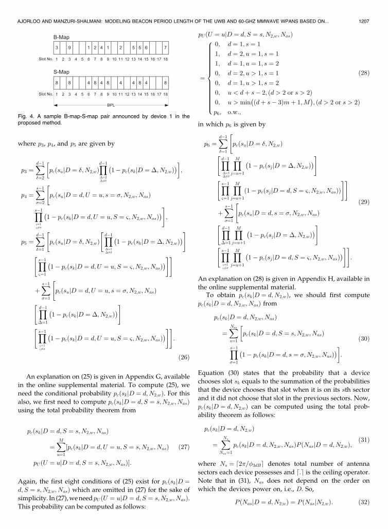


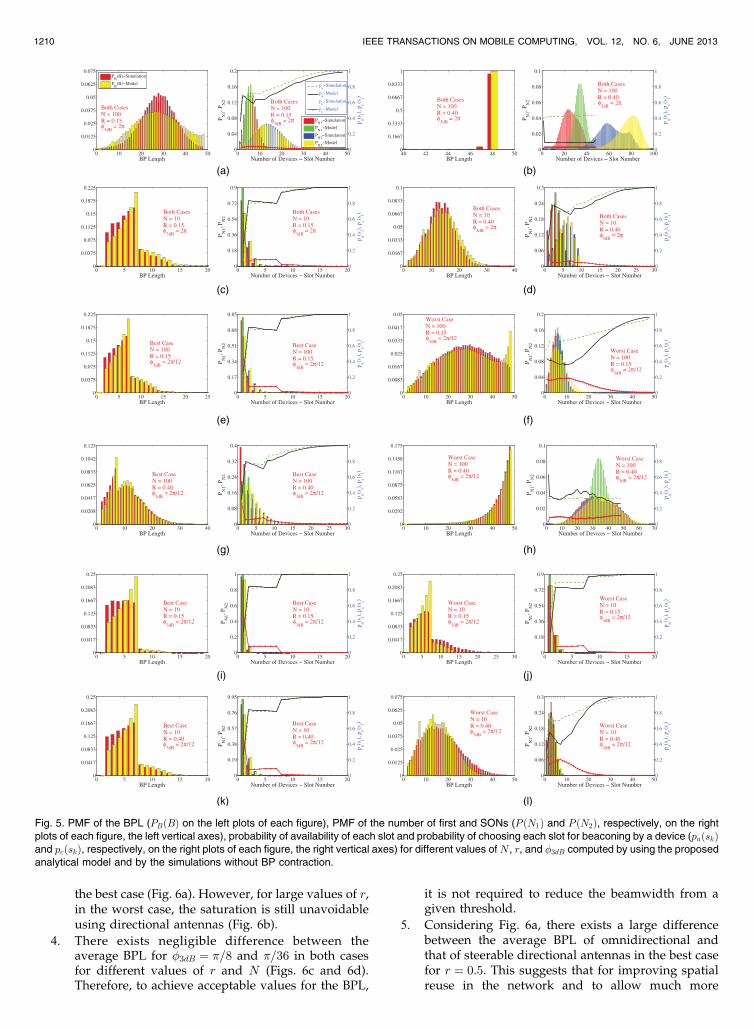


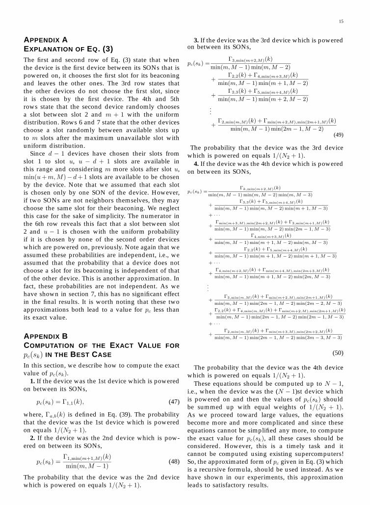
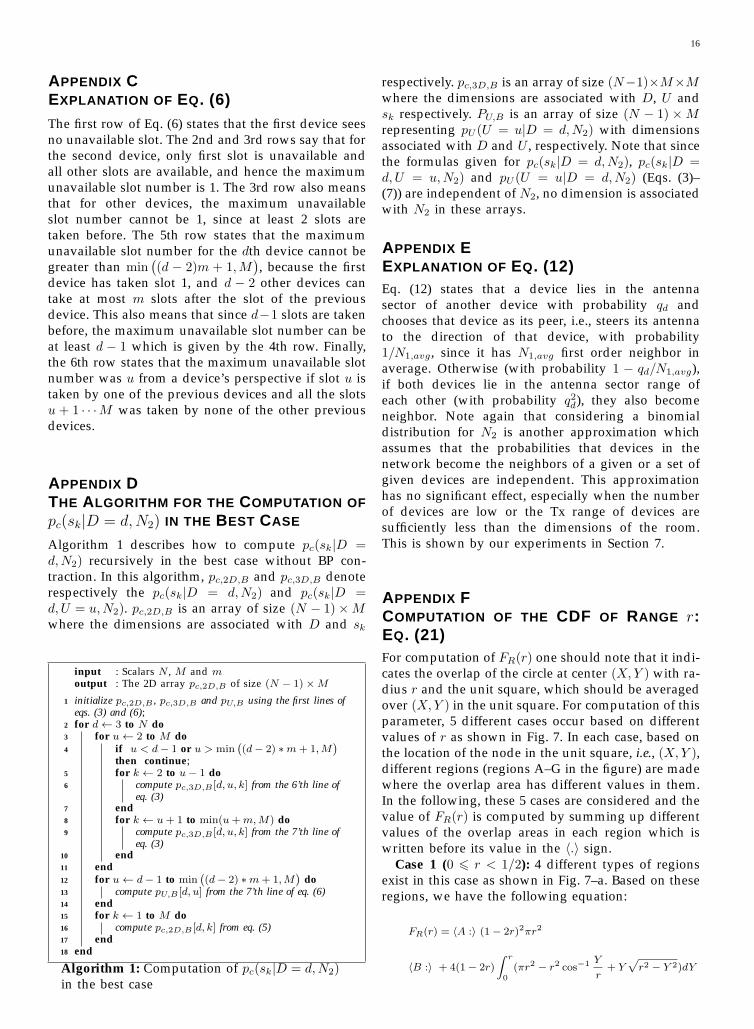
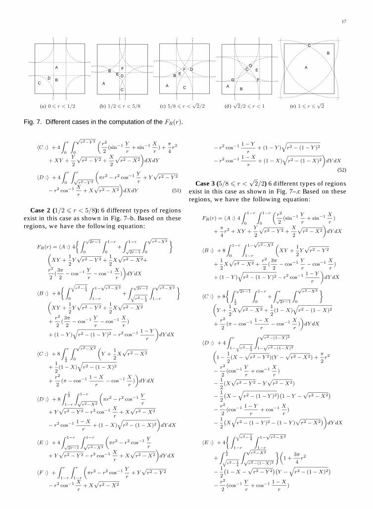

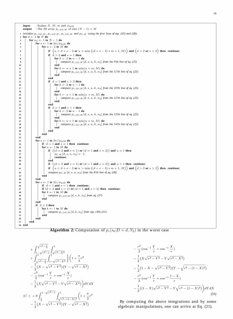
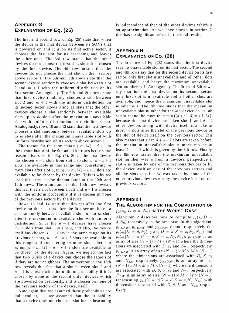

![[MS-WPE376]: WordPad ECMA 376 Standards Support · WordPad ECMA 376 Standards Support](https://static.documents.pub/doc/80x56/5fab533dea0e1c27ad282e55/ms-wpe376-wordpad-ecma-376-standards-support-wordpad-ecma-376-standards-support.jpg)


