Modeling bubble heat transfer in gas–solid fluidized beds using DEM

Amit V. Patil, E.A.J.F. Peters n, T. Kolkman, J.A.M. KuipersMultiphase Reactors Group, Department of Chemical Engineering & Chemistry, Eindhoven University of Technology, P.O. Box 513, 5600 MB Eindhoven,Netherlands

A U T H O R - H I G H L I G H T S

� Non-isothermal Discrete Element Method is implemented and validated.� Results for non-isothermal bubble injection in a gas–solid fluidized bed are presented.� HTC's for bubbles as a function of particle sizes and injection temperature is computed.� Results are compared well with the Davidson and Harrison model for bubble HTC's.

a r t i c l e i n f o

Article history:Received 5 September 2013Received in revised form29 October 2013Accepted 2 November 2013Available online 11 November 2013

Keywords:Fluidized bedsDiscrete Element MethodHeat transfer coefficientDavidson and Harrison bubble model

a b s t r a c t

Discrete element method (DEM) simulations of a pseudo 2-D fluidized bed at non-isothermal conditionsare presented. First implementation details are discussed. This is followed by a validation study whereheating of a packed column by a flow of heated fluid is considered. Next hot gas injected into a colderbed that is slightly above minimum fluidization conditions is modeled. In this study bubbles formed inmonodisperse beds of different glass particle sizes (1 mm, 2 mm and 3 mm) and with a range of injectiontemperatures (300–900 K) are analyzed. Bubble heat transfer coefficients in fluidized beds are reportedand compared with values produced by the Davidson and Harrison model.

& 2013 Elsevier Ltd. All rights reserved.

1. Introduction

Fluidized beds with gas–solid flows are used in a variety ofindustries due to their favorable mass and heat transfer character-istics. Some of the prominent processing applications includecoating, granulation, drying, and synthesis of fuels, base chemicalsand polymers.

Industrial scale fluidized beds working in the bubbling regimehave many gas bubbles forming and rising inside the emulsionphase. Many such gas bubbles collectively affect the overall heatand mass transfer rate and thus affect the overall performance ofthese contactors. Depending on the nature of reactions, i.e.,whether they are exothermic or endothermic, fluidized particlesheat exchange takes place from the emulsion to bubble phase orvice versa.

Hot gas, such as air or steam, is often injected using spouts influidized beds for processes such as coal gasification, see Xiao et al.(2006), Weber et al. (2000) and Ye et al. (1992). Since inlet gas

temperatures are different from the bed temperatures of fluidizedbeds, the bubble phase is at a different temperature compared togas–solid emulsion phase in fluidized beds.

Until recently computational research for fluidized beds waslimited to hydrodynamics of the bed. Now, with the properunderstanding of the hydrodynamics, the frontier has movedtowards heat transfer in fluidized beds. This work focuses onmodeling of this heat transfer in fluidized beds using the discreteelement model (DEM) approach. One reason to choose a computa-tional approach instead of an experimental one is that techniquesfor obtaining energy profiles in fluidized beds without perturbingthe system, e.g., by inserting probes are not readily available.However DEM has the capability to provide all hydrodynamic andthermal properties with ease and reasonable accuracy.

The hydrodynamics of gas–solid flow in DEM is modeled bytreating the gas phase as a continuum (Eulerian) and particulatephase as discrete (Lagrangian). Through two-way-coupling boththe continuum and particulate phase interact with each otherthrough momentum exchange. The particulate mechanics forcollision used in this study is based on the soft sphere model firstproposed by Cundall and Strack (1979). To the DEM hydrodynamicmodel developed by Hoomans et al. (1996), the energy balance for

Contents lists available at ScienceDirect

journal homepage: www.elsevier.com/locate/ces

Chemical Engineering Science

0009-2509/$ - see front matter & 2013 Elsevier Ltd. All rights reserved.http://dx.doi.org/10.1016/j.ces.2013.11.001

n Corresponding author. Tel.: þ31 40 247 3122; fax: þ31 40 247 5833.E-mail address: e.a.j.f.peters@tue.nl (E.A.J.F. Peters).

Chemical Engineering Science 105 (2014) 121–131

modeling heat transfer is added where the continuous phase ismodeled by a convection–conduction equation and the discretephase is treated using an average temperature for each particle.

A DEM with heat transport implementation has been reportedin previous studies (Zhou and Zulli, 2009; Zhou et al., 2010). Thesestudies focus on the overall heating of beds which includesevaluation of overall heat transfer coefficient of the beds. Thecurrent work, however, focuses on the heat transfer of risingbubbles in fluidized beds. Although isothermal bubble formationand rise in fluidized beds have been studied by Caram and Hsu(1986), Nieuwland et al. (1996) and Davidson and Harrison (1966),non-isothermal effects were not considered in these studies.

Previously, mainly experiments have been performed to studyheat transfer in rising bubbles in fluidized beds, e.g., by Wu andAgrawal (2004). These experiments have proposed heat transfercoefficients for rising bubbles in fluidized beds for smaller parti-cles in the range 250–500 μm. However, no DEM or othersimulation-based study has been performed on such systems untilnow. In the current work also heat transfer coefficients of bubblesin fluidized beds are predicted. The obtained heat transfer coeffi-cient values compare well with the theoretical Davidson bubblemodel given in the literature (Kunii and Levenspiel, 1991;Davidson and Harrison, 1963) for smaller particles with deviationsfor larger particles. An analogous experimental work lookingat mass-transfer has been performed (Dang et al., 2013), but thecurrent work is the first of its kind concerning heat transfer.

Heat transfer in fluidized beds can be studied by three mainmodeling methods. They are the direct numerical simulations,discrete element method and the two fluid model. The directnumerical simulation (DNS) which is a highly resolved gas–solidflow study is suited for small scale where studies like bubbleinjection is not feasible because of expensive computations. Thetwo fluid model has a lower flow resolution and needs manyclosure relations from DNS. Thus we choose DEM which is bestsuited for a pseudo-2D bed study and has adequate scale for singlebubble injection.

We will start with stating the governing equations in Section 2and provide details of their implementation in Section 3. Thedeveloped heat transport implementation is verified by compar-ison with analytical solutions before being put to use for thefluidized bed study in Section 4. The system used for thisverification is a packed bed being heated up by a hot stream.Using the developed DEM model bubble injection simulations of a2D bed were performed. The bubble injection is performed byspecifying the proper boundary conditions at a nozzle or spout atthe bottom of the bed. In the simulations different injectiontemperatures and particle sizes are used. This work presents astudy of the formation and rise of hot gas bubbles in beds. Thebubble injection mass flux through the nozzle is fixed to observethe changes in the formed bubble due to temperature. Heattransfer coefficient is determined from the simulations and com-pared with theoretical predictions.

2. Governing equations

2.1. Gas phase modeling

In our model the gas phase is described by volume averagedconservation equations for mass and momentum given by

∂∂tðɛfρf Þþ∇ � ðɛfρfuÞ ¼ 0; ð1Þ

∂∂tðɛfρfuÞþ∇ � ðɛfρfuuÞ ¼ �ɛf∇p�∇ � ðɛf τf ÞþSpþɛfρf g; ð2Þ

where Sp represents the source term for momentum from theparticulate phase and is given by

Sp ¼∑a

βVa

1�ɛfðva�uÞδðr�raÞ �α�βu: ð3Þ

In the right-most equation only β remains as a factor in front ofthe gas velocity due to the definition of the solid-volume fraction(that equals 1�ɛf ) and α collects all momentum creation per unitvolume due to the velocities of the particles. After discretizationsmoothed Dirac-delta functions are used to distribute particleproperties over nearby grid-points. The drag coefficient, β, isevaluated by the Ergun (1952) equation for dense regime andWen and Yu (1966) equation for dilute regimes

Fdrag ¼βd2pμ

¼150

1�ɛfɛf

þ1:75ɛs Rep if ɛf o0:8

34CD Repð1�ɛf Þɛ�2:65

f if ɛf 40:8

8>>><>>>:

ð4Þ

The viscous stress in Eq. (2) is taken to be the usual Newtonianstress expression:

τf ¼ �μð∇uþð∇uÞT Þ�ðλ�23 μÞð∇ � uÞI;with ∇ � ðɛf τf Þ � �Qu: ð5Þ

Here the operator Q is introduced for notational convenience.The thermal energy equation for the fluid is given by

∂ðεfρf Cp;f TÞ∂t

þ∇ � ðεfρfuCp;f TÞ ¼∇ � ðεf kefff ∇TÞþQp; ð6Þ

where Qp represents the source term from interphase energytransport and kefff is the effective thermal conductivity of the fluidphase that can be expressed in terms of fluid thermal conductivityas

kefff ¼ 1� ffiffiffiffiffiffiffiffiffiffiffiffi1�εf

pεf

kf ð7Þ

This equation was first proposed by Syamlal and Gidaspow (1985)and later used in many works such as Kuipers et al. (1992) andPatil et al. (2006). The source term due to the heat-transfer of theparticles to the fluid can be obtained by summing the contribu-tions of all particles using a (smoothed) delta-function as

Qp ¼ �∑aQaδðr�raÞ ¼∑

ahfpAaðTa�Tf Þδðr�raÞ: ð8Þ

Here Qa is the heat transferred from the fluid to particle a. It can beexpressed using a temperature difference and a heat-transfercoefficient (see next section).

2.2. Discrete particle phase

The solid phase is considered to be discrete. The modelingof the particle phase flow is based on tracking the motion ofindividual spherical particles. The motion of a single sphericalparticle a with mass ma and moment of inertia Ia can be describedby Newton's equations:

mad2radt2

¼ �Va∇pþβVa

1�ɛfðu�vaÞþmagþFcontact;a ð9Þ

Iad2Θa

dt2¼ τa ð10Þ

where ra is the position. The forces on the right-hand side ofEq. (9) are due to the pressure gradient, drag, gravity and contactforces due to collisions, τa is the torque, and Θa the angulardisplacement.

The heat transfer to the particles from the fluid is modeledfor DEM by interpolation of the gas temperatures given at grid-points to obtain a temperature, Tf, at the particle position. Theheat balance for particle a gives an evolution-equation for its

A.V. Patil et al. / Chemical Engineering Science 105 (2014) 121–131122

temperature, Ta:

Qa ¼ ρaVaCp;pdTa

dt¼ hfpAaðTf �TaÞ ð11Þ

where hfp is the particulate interfacial heat transfer coefficient forwhich we use the empirical correlation given by Gunn (1978):

Nup ¼ ð7�10εf þ5ε2f Þ½1þ0:7 Re0:2p Pr0:33�þð1:33�2:40εf þ1:20ε2f Þ Re0:7 Pr0:33 ð12Þ

where

Nup ¼hfpdpkf

; Rep ¼dpεfρf ju�vj

μfand Pr¼ μf Cp;f

kf: ð13Þ

3. Numerical solution methods

3.1. Gas phase

Firstly we apply time discretization to the gas-phase equations(1), (2) to obtain

½ɛfρf �nþ1�½ɛfρf �nΔt

¼ �½∇ � ðɛfρfuÞ�nþ1 ð14Þ

½ɛfρfu�nþ1�½ɛfρfu�nΔt

¼ �½∇ � ðɛfρfuuÞ�n�ɛnf ∇pnþ1þQ n

dunþ1

þ½Q ou�n�βnunþ1þαnþ½ɛfρf g�n ð15Þ

In this scheme the operator Q of the viscous stress term as definedin Eq. (5) is split into two parts. The part Q d contains the diagonalpart of the operator needed to compute the shear stress, i.e.,

Q d ¼∇ � ½ɛfμ∇�þdiagð∇½ɛfμ∇��Þ ð16Þand the remainder is put into Q o ¼Q�Q d. Taking part of theviscous stress implicitly gives extra stabilization to the schemeallowing for the use of larger time steps.

Eq. (15) is solved by means of the two-step projection algo-rithm originally developed by Chorin (1968). First an ‘intermedi-ate’ velocity, un, is computed as

ð½ɛfρf �n�ΔtQ ndÞun ¼ ½ɛfρfu�nþΔtð�½∇ � ðɛfρfuuÞ�n

þ½Q ou�nþαnþ½ɛfρf g�nÞ ð17Þ

This requires the solution of a linear matrix-vector equation. Usingthis velocity the second term in Eq. (15) can be written as

½ɛfρfu�nþ1 ¼ ½ɛfρf �nunþΔtð�ɛnf ∇pnþ1þQ n

dðun�unþ1Þ�βnunþ1Þð18Þ

The equation that is solved is this one, but with the termΔtQ n

dðun�unþ1Þ, which is second order in Δt and can beneglected. The term ðun�unþ1Þ is a function of Δt and becomessmall for small Δt. The resulting scheme is very stable and firstorder. Inserting that expression into the continuity equation weobtain a equation for the pressure, where the density is computedby the ideal gas law: ρf ¼ ðM=RTÞp. Then we solve unþ1 and pnþ1

iteratively by

unþ1;kþ1 ¼½ɛfρf �nun�Δtɛnf ∇p

nþ1;k

ɛnþ1f ρnþ1;k

f þβn ð19Þ

�∇ � ðɛnf ∇pnþ1;kþ1Þþɛnþ1f M

RTnþ1Δt2pnþ1;kþ1

¼ �∇ � ½ɛfρf �nun

Δt�βnunþ1;kþ1

!þ½ɛfρf �n

Δt2ð20Þ

Here superscript k indicates the iteration step and initial values areunþ1;0 ¼ un and pnþ1;0 ¼ pn.

Similar to the evolution equations of the hydrodynamic fieldsconvection–conduction equation for the temperature, Eq. (6), issolved using a semi-implicit scheme:

ðεfρf Cp;f �∇ � ðεf kefff ∇ÞÞTnþ1f ¼ ðεfρf Cp;f T f Þn�Δtð∇ � ðεfρfu

nHf Þ�QpÞ:ð21Þ

Because here the gas-velocities at time t¼n are used and inEq. (20) the temperature at the new time is required, first Eq. (21)and next Eqs. (19), (20) are solved.

For the spatial discretization a uniform Cartesian staggered gridis used. The second order dissipative terms, such as the viscousterms and heat conduction, are approximated using centraldifferences. For the convective terms the min-mod total variationdiminishing (TVD) scheme is used (Roe, 1986).

To complete the set of equations boundary conditions areenforced on the velocities (normal and tangential directions),pressure and temperature. In the implementation of these bound-ary conditions the value of the quantity at a ‘boundary cell’ is used.Fig. 1 shows where the different quantities inside the cell aredefined. A boundary cell quantity, ϕb, is represented as a linearcombination of at most 2 neighbouring relevant inner cells (ϕ1

and ϕ2):

ϕb ¼ aϕ1þbϕ2þc: ð22ÞIn the case of first order boundary conditions, as presently used,b¼0. For influx boundaries the value in the boundary cell is setequal to the incoming value (a¼0, b¼0, c¼ϕin). For boundarieswhere the value is set, but there is no influx we use linearinterpolation. This gives a¼ �1, b¼0 and c¼ 2ϕwall, for a cell-centered quantity. The method of evaluation of coefficients hasbeen discussed in more detail in Deen et al. (2012).

For some of the steps in the numerical scheme a linear set ofequations needs to be solved, namely, for Eqs. (17), (20), (21). In allthese cases the matrices involved are positive definite symmetric.Furthermore, due to the Cartesian grid used they have a simplebanded structure. A highly efficient solver that applies the con-jugate gradient method with an incomplete Cholesky precondi-tioner (ICCG) is used to solve these equations. A similarimplementation as applied here for the fluid phase in DEM hasbeen presented by Deen and Kuipers (2013) for DNS immersedboundary simulations.

3.2. Discrete particle phase

As mentioned earlier the particle collision mechanism treatedhere comes from the Cundall and Strack (1979) spring dashpotmodel for particle collision. Along with collision forces all remain-ing contributions of forces coming from drag, gravity and pressuregradient are summed up to get the total force acting on eachparticle. Using the total force, parameters of particles acceleration,velocity and position are evaluated and updated every DEMtime steps.

The integration method used for this operation is the first orderexplicit integration which has been described earlier in the

Fig. 1. The thick solid line is the boundary. The cell with the dotted perimeter tothe left is a boundary cell and to the right are internal cells. Due to the use of astaggered grid quantities are defined at different positions.

A.V. Patil et al. / Chemical Engineering Science 105 (2014) 121–131 123

literature (Hoomans et al., 1996). This is one of the simplest ofintegration methods compared to many number of methods thathave been developed like the Gear and Verlet family of algorithms(Ye et al., 2004). The normal and tangential spring stiffness foreach of the particle sizes are chosen such that under the givenconditions the maximum particle overlap is always less than 1% ofthe particle diameter, for maximum particle relative velocity of1 m/s. Generally in simulation like these relative velocities are lessthan 0.6 m/s therefore an overlap of more than 1% occurs only veryrarely.

Details of these calculations are provided in Cundall and Strack(1979) which also gives the maximum contact time of particlesduring collision. The DEM time step size is set such that it is notless than 1/5 the contact time. The value chosen in these simula-tion is 1/10 the contact time. Thus the Eulerian time step size canbe evaluated which here is taken to be 10 times the Lagrangiantime step size.

4. Implementation test and verification

In this section a verification of the heat transfer couplingimplementation is provided. Tests for the hydrodynamics havealso been performed, but are not presented because they are verysimilar to verifications found in the literature, such as van SintAnnaland et al. (2005). The system that is considered is a fixed bedof initially cold liquid and cold particles that is heated up by a flow

of hot fluid. The hot fluid passes through the fixed bed from thechannel inlet. Thus the temperature of the fluid in the bed risescausing the fixed particles to heat up too.

For the heat transfer test we choose water as fluid and copperas solid particles. The domain size, particle size, particle arrange-ments and water properties assumed for the test are the same asthe Ergun equation test in van Sint Annaland et al. (2005).The Ergun equation test of van Sint Annaland et al. (2005)validates the hydrodynamics which was once again repeated herebut not discussed. Instead here only the heat transfer validation ispresented. The arrangement of particles here is a primitive cubicsystem with particle spacing of 0.05 mm with a bed porosity of0.4935. The hydrodynamic and thermal properties used aretabulated in Table 1.

The model verification is done by using a one dimensionalconvection equation with heat-exchange between the fluid andthe particle phase. Thermal conduction terms are neglected asthey are bound to be small at high enough Péclet number. Forthe chosen settings the Péclet number equals Pé¼83,740. For the1-dimensional model the gas phase energy and particle phaseenergy balance, respectively, are given by

ɛfρf Cp;f∂Tz

∂t¼ �ɛfρuzCp;f

∂Tz

∂z�haðTz�TzpÞ; ð23Þ

ɛpð1�ρf ÞCp;p∂Tzp

∂t¼ haðTz�TzpÞ; ð24Þ

where a is the specific interfacial area given by a¼ 6ð1�ɛf Þ=dp.By integrating Eqs. (23), (24) with appropriate initial and boundaryconditions we can get the analytical equations for the givensystem. The details of the analytical solution method for heattransfer can be found in references Anzelius (1926), Bateman(1932), Hougen and Watson (1947) and Bird et al. (2001). Fig. 2shows the evolution of the temperature profile through the bed ofthe particle phase at several instances in time. In the plot thesimulation results are compared with the analytical solution. Alsothe results of a highly refined grid 1-D discretized simulation ofthe model Eqs. (23), (24) are shown. The agreement between theDEM heat-transfer code and the solutions of the 1-D approxima-tion is very close, as is to be expected in this case. For the profilesof the fluid temperature, not shown here, we found an equallygood correspondence. From this test (among others not reportedhere) we conclude that the code is well verified.

Table 1Properties and grid settings used in the fixed bedverification study.

Stationary particle array 25�25�125Channel diameter 0.1 mChannel length 1.0 mParticle diameter 3.95 mmLiquid density 1000 kg/m3

Liquid viscosity 0.001 Pa sLiquid inlet velocity 0.1 m/sParticle density 8400 kg/m3

Liquid thermal conductivity 0.5 W/mKLiquid heat capacity 4187 J/kg KParticle heat capacity 385 J/kg K

Fig. 2. Unsteady state evolution of the temperature in a bed filled with cold liquid and particles that is heated up by a liquid flow. The graphs show the temperature profilealong the bed length of the copper particles at several instances in time. Good correspondence is found between the DEM simulation results and the solutions (numericaland analytical) of a 1-D approximate model.

A.V. Patil et al. / Chemical Engineering Science 105 (2014) 121–131124

5. Bubble formation and rise by hot gas injection

The main results presented in this section concern singlebubble injections in a pseudo-2D fluidized bed. Hot gas is injectedthrough an incipiently fluidized bed. For the incipient fluidizationthe background gas is maintained slightly above the minimumfluidization velocity and the temperature of this background gas iskept at 300 K in all the simulations. The boundary conditions usedare shown in Fig. 3. A central injection nozzle with a set inlet massflux (see Table 2(b)) is used to generate a gas bubble in the bed.After a time of about 0.18 s the bubble necks and pinches off.

At that time the hot-gas injection is stopped. Cold gas with thesame background velocity as elsewhere now flows from the nozzleand the bubble rises in the fluidized bed.

Table 2(a) summarizes the properties of the gas and particlesthat were used in the simulation. There were 3 sizes of glassparticles used: 1 mm, 2 mm and 3 mm. These particles are of typeD in the Geldart classification. For each of the particle sizes a rangeof injected gas temperature were considered, all at the same massflux. The particle collision parameters and fluidization velocitiesused for these simulations are shown in Table 2(c). Cundall andStrack (1979) give details of how the spring stiffness parameters

Fig. 3. The computational domain divided into grid cells with cell flag (as in the simulation code) that indicate the used boundary conditions. Flags: 1: internal, 2/3: no-slip/adiabatic, 4: prescribed fixed influx, 5: prescribed pressure/zero normal temperature gradient, 7: corner cell, 12: prescribed nozzle influx. (a) Hydrodynamics. (b) Heat-transfer.

Table 2Settings used for bubble-injection DEM simulations.

(a) Global

Particle type glassρp 2526 kg/m3

Norm. coeff. of restit. 0.97Tang. coeff. of restit. 0.33Cp;f 1010 J/kg KCp;p 840 J/kg KΔt (Eulerian) 2.5�10�5 sΔt (Lagrangian) 2.5�10�6 s

(b) Different for each temperature

Mass flux (kg/m2 s) T (K) ρf (kg/m3) uinj (m/s)

17.55 300 1.1700 15.0500 0.7020 25.0700 0.5014 35.0900 0.3901 45.0

11.7 300 1.1700 10.0500 0.7020 16.67700 0.5014 23.33900 0.3901 30.0

(c) Different for each particle size

dp (mm) ubg (m/s) Norm. spring stiffness (N/m) Tang. spring stiffness (N/m) Bed size (m�m�m) Grid size

1 0.6 7000 2248.9 0.21�0.010�0.6 30�2�802 1.1 10,000 3212.7 0.21�0.015�0.6 30�2�803 1.45 19,000 6104.1 0.21�0.018�0.6 15�2�80

A.V. Patil et al. / Chemical Engineering Science 105 (2014) 121–131 125

given in Table 2(c) are used and implemented in the collisionmodel. Table 2(b) gives the respective gas densities and back-ground velocities used for the simulations at each temperature.

The pseudo 2D-bed has a width of 21 cm and a depth that isdifferent for different particle sizes (see Table 2(c)). Through thecentral injection nozzle, with width 1.4 cm (and depth equal to thebed depth) air at different temperatures and ambient pressure isinjected. The temperatures considered are 300–900 K. The massdensity and inlet velocities directly follow from the ideal gas-law(see Table 2(b)).

Fig. 4 shows snapshots of a dynamic bubble formation and risethrough the incipiently fluidized bed. The injection temperature is

700 K here. This figure shows how the temperature profile devel-ops inside a rising gas bubble. As can be observed after theinjection stops at 0.18 s the bubble rises though the fluidized bedwith hot spots forming on the sides of the bubble. As thetemperature of gas in the bubble reduces quickly a new tempera-ture scale is used for each snapshot.

The gas that is in contact with the emulsion phase quickly coolsdown to 300 K due to the efficient heat-transfer to the particles.Since the glass particles have a high heat capacity per unit volumerelative to the air, their temperature does not rise much.

After injection has stopped the hottest part of the gas is nearthe sides of the bubble. The hot gas tends to accumulate herebecause the low background temperature gas moves up throughthe center of the bubble. Part of the gas moves down along theperimeter of the bubble. The particles that are heated at the top ofthe bubble also move down along the perimeter. They end up inthe wake of the bubble where they will heat up the gas passingthrough the middle creating a plume as seen at t¼0.3 s and moreclearly at t¼0.4 s in Fig. 4.

The temperature field along with the gas velocity field att¼0.3 s that is shown in Fig. 5(a) gives a better understanding ofthe temperature distribution in a bubble. It shows how thebackground gas, that is used to keep the bed fluidized, flowsthrough the bubble creating a natural tendency for the hot pocketsto move to the sides. In Fig. 5(b) the theoretical streamlinesaccording to the model of Pyle and Rose (1965) are shown (seealso Davidson and Harrison, 1963). For bubble velocities, Ub,smaller than the interstitial velocities, u0 ¼ umf=ɛmf , there aresmall circulation zones near the side. The (hot) gas in thesezones remains there. The heat can only escape by conduction.This is qualitatively consistent with what is seen in the simulations(Fig. 5(a)).

In our simulations the background gas velocity is slightly largerthan the minimum fluidization velocity. Therefore we can estimateu0 � ubg=ɛmf , where we take the porosity ɛmf of emulsion phase at

Fig. 4. Snapshots at different times of gas injected at 700 K in a 300 K incipientlyfluidized bed. The injection mass flux is 11.7 kg/m2 s. At 1.8 s the injection isstopped. Note that the temperature scales are different for particles and gas andalso change for each snapshot. Due to the high heat capacity per unit volume of thesolids, the gas quickly cools down and the particles only warm up several degrees.For t¼0.2 s and 0.3 s hotter side pockets are seen in the bubbles. For t¼0.3 s and0.4 s particles in the bottom zone heat the gas that passes through it, which givesrise to the hotter plume in the middle.

Fig. 5. A detailed view of a bubble at time t¼0.3 s for a 700 K injection temperature in a 2 mm size particle bed. The injection mass flux is 11.7 kg/m2 s. The left picture in(a) shows the temperature fields of gas and particles. The right picture shows the porosity field and the flow field. The background gas flows through the middle of thebubble. At the sides one sees a small circulation zone. This explains the two side pockets of hotter air. These circulation zones are predicted by the classic theories from Pyleand Rose (1965) and Davidson and Harrison (1963). The streamlines, in the reference frame moving with the bubble, are shown in (b) which is adopted from Pyle and Rose(1965). (a) Simulation. (b) Theory.

A.V. Patil et al. / Chemical Engineering Science 105 (2014) 121–131126

minimum fluidization to be 0.5. The mean bubble rise velocity, Ub,was calculated for the simulation presented here by monitoringthe displacement of the centre of the bubble area with time.Table 3 gives the ratio obtained for different particle sizes from thepresent simulation. It is seen that all our simulations fall inside theregime corresponding to Fig. 5(b) (i.e., u0=Ub41).

Fig. 6 shows the effect of particle size on the formation of thebubbles. It can be observed in this figure that, as particle sizechanges for the same injection temperature and injection massflux, the bubble size is different. For smaller particles the perme-ability of the emulsion phase is less causing a weaker leakage ofgas and heat thus forming a larger bubble and more heatremaining within the bubble. Also, for the smaller particle sizethe hot size pockets in the bubble are larger. This is consistent withthe values reported in Table 3 and the theoretical streamlines inFig. 5(b). For smaller particles the circulation zones are larger.

In Fig. 7 snapshots of bubbles at the same instances in time(i.e. t ¼ 0:2 s, 0.3 s and 0.4 s) created with air injected at differenttemperatures are depicted. The particle size in each of thesesimulation snapshots is the same, namely, 2 mm. The amount ofgas injected in terms of mass is the same, so this corresponds tothe same volume once cooled down to 300 K. The fact that theobserved bubble is bigger for the higher temperatures can beexplained by the fact that the injection velocity is higher. Thismeans that the amount of momentum and kinetic energy suppliedby the injection is larger for higher temperatures. When compar-ing the different bubbles at the same time it is noticed that thebottom positions are the same. The difference is in the rainingdown of the particles from the ceiling. The gas temperaturedistribution is similar, mainly the magnitude differs.

In Fig. 8 the time-evolution of an effective bubble diameterfor several injection temperatures and particle sizes is shown. Thisdiameter is computed from the bubble volume expressed as acylinder (quasi-2D) with this diameter. To compute the volume thebubble was traced using the average porosity in a grid cell.A threshold of 0.75 was used for this.

The graphs initially show a linear growth. Note that the gasinjection is stopped at t¼0.18 s, but the bubbles still grow some-what after that time. Beyond, say, t¼0.25 s the bubble sizes arenearly constant. Note, however, that the data-points at later timesare less trustworthy because of the difficulty of defining thebubble volume when particles are raining down from the roof ofthe bubble. The bubble size for isothermal injection at 300 K in theplot of Fig. 8 matches well with results previously published in theliterature (Olaofe et al., 2011).

Bubbles are larger for higher injection temperatures andsmaller particle sizes. For larger particles the resistance of the airflowing in and out of a bubble is less. Therefore the gas-leakageout of the bubble is larger for systems with larger particles andbubble sizes will be smaller. The graphs in Fig. 8 also show that thebubble size increases with injection temperature. The reason isthat for equal mass flux, higher temperatures mean higher volumeflux and thus larger gas velocities. This gives a higher gasmomentum, which is partly transferred to the particle movingoutward and thus forming a larger bubble.

Table 3The interstitial velocity, u0, in emulsion phase compared to the bubble rise velocity,Ub.

dp (mm) u0 Ub u0=Ub

1 1.16 0.8 1.452 2.2 0.5 4.43 2.8 0.4 7

Fig. 6. Gas bubble formation and rise with 900 K injection temperatureand different particle sizes. The injection mass flux is 11.7 kg/m2 s. Withincreasing particle size the hot side pockets decrease in size and the hot plumein the middle becomes more pronounced. (a) time t¼0.1 s. (b) time t¼0.3 s.(c) time t¼0.4 s.

A.V. Patil et al. / Chemical Engineering Science 105 (2014) 121–131 127

The mean temperature of the bubble with respect to timeis shown in Fig. 9. Let us focus on the 900 K case in Fig. 9(a) fordifferent particle sizes. It is seen that initially the temperature att¼0.1 s in the 1 mm particle bed is smallest. The reason is that forthese small particles the gas leakage out of the bubble is least. Thismeans that hot gas, that is cooled down by the particles, remains(partially) in the bubble. It will flow downward past the sides ofthe bubble where it is cooled by the particles. This decreases thetemperature almost immediately. For the larger particles, initially,most of the gas inside the bubble is the hot gas directly injectedinto it. Therefore, initially, the bubble temperature is nearly equalto the injection temperature for the larger, 3 mm, particle system.

After this initial stage, while still injecting hot gas, there is muchmore leakage in and out of the bubble in case of the larger particles.In fact there is a flow that transports cold background gas into thebubble. This mixing in of cold gas causes the temperature inside thebubble to decrease quicker for the large particles. For the smallerparticles hot gas partly circulates and less background gas enters inthe bubble such that more of the heat is retained.

When the injection is stopped the temperature initially dropsvery fast. This drop is largest for the large particle systems. Thereason is that the hot gas (at the top) leaks out quickly and coldbackground gas enters. Due to the stagnant character of theremaining warm zones the cooling down after the initial quickdrop is much slower.

A simple energy balance for the gas inside the bubble, after theinjection has stopped, is

ρf VbCp;fdTb

dt¼ �hbAbðTb�TeÞ; ð25Þ

where Te is the temperature of the emulsion phase. Here it isassumed that the heat transfer from the bubble to the emulsionphase can be described well by a constant heat-transfer coeffi-cient. Furthermore it is assumed that the size of the bubble doesnot change much, which seems to be valid after t¼0.25 s as seenfrom Fig. 8. The analytical solution of this equation gives expo-nential decay according to

TbðtÞ�Te

Tbðt0Þ�Te¼ exp

�hbAbðt�t0Þρf VbCp;f

" #: ð26Þ

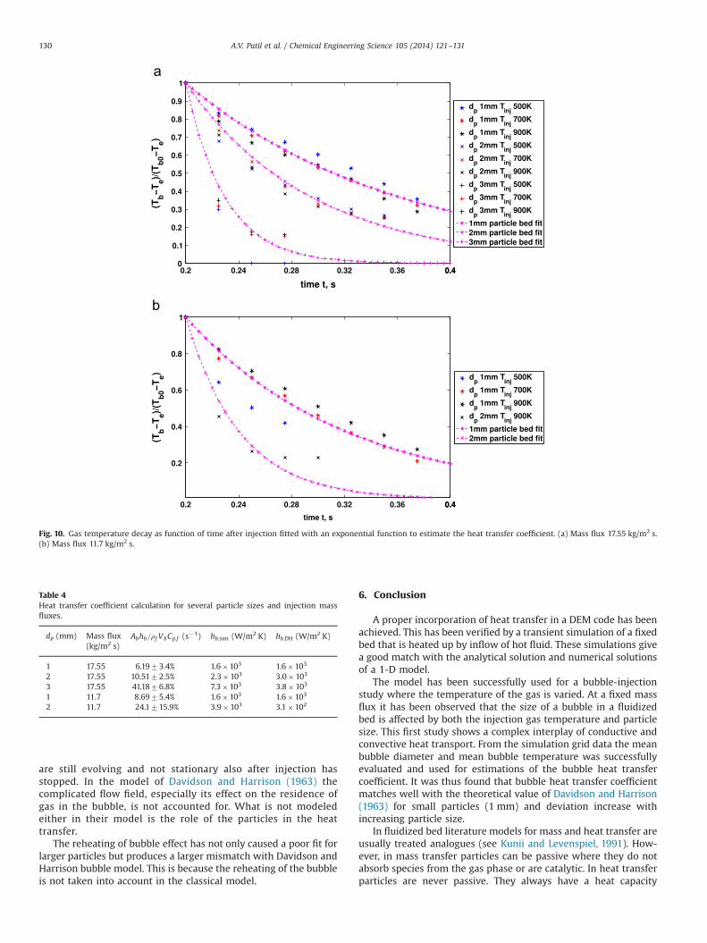
In Fig. 10 the measured temperature decay, after injection hasstopped (t0¼0.2), is fitted to exponentials. The decays for alltemperatures are fitted simultaneously. For the mass flux of11.7 kg/m2 s we have considered only the two smaller particlesizes, because for the 3 mm case the decay is so fast we could notobtain accurate numbers. The reason is that in that case Tbðt0Þ�Te

is too small and dominated by fluctuations.The mean bubble dimensionless temperatures does not fully decay

to zero for the 2 and 3 mm particles in Fig. 10. This is because the hotparticles from the side boundary are continuously collecting in thewake of the bubble and heat the cold gas-stream entering the bubblefrom below. This causes a small resupply of heat to the bubble thoughit is loosing heat from the top thus reducing the decay rate of themean temperature of the bubble. In our fitting this phenomena ofreheating of bubble was not taken into account because we explicitlyassume a decay to zero. It might, however, explain the relatively poorquality of the fit for the larger particle sizes.

From the values of the exponential decay we can find a heat-transfer coefficient. All the needed quantities can be obtained formthe DEM simulation. For the bubble area Ab we used the area of acylinder corresponding to the diameter in the plateau regime of Fig. 8.The value obtained for the heat-transfer coefficients can be comparedto models. When performing the fit the data obtained for differenttemperatures, made dimensionless as in the right-hand-side ofEq. (26), was lumped together. Besides this also an average bubblediameter was taken to convert the decay time to a interfacial heat-transfer coefficient. The values obtained are reported in Table 4.

For our comparison we use the model of Davidson and Harrison(1963) and also presented in Kunii and Levenspiel (1991). In thismodel transfer from the bubble to the emulsion phase takes placeby two mechanisms which are convective flux due to inlet back-ground gas flow and heat conduction from the bubble to emulsiondue to temperature gradients. The latter term is expected to beweak in our case and convective transport is the dominantmechanism determining the heat transfer coefficient. The detailedderivation of the convective and conduction terms are provided inDavidson and Harrison (1963) in terms of mass-transport (Appen-dices A.2 and C) and is not described here.

For a cylindrical bubble Davidson and Harrison (1963) find thatthe flow rate through the bubble is 2ubgdp times the bed depth. Thismeans that the average velocity through the projected area of thebubble is twice ubg. (For a 3D bubble the factor is 3.) By assumingideal mixing inside the bubble we get the convective part ofthe heat-transfer coefficient in this model. The full heat-transfercoefficient including the conductive part according to Davidson and

Fig. 7. Gas bubble rise with varying injection temperature and same particle size of2 mm and with the same injection mass flow of 11.7 kg/m2 s. (a) Time t¼0.2 s.(b) Time t¼0.3 s. (c) Time t¼0.4 s.

A.V. Patil et al. / Chemical Engineering Science 105 (2014) 121–131128

Harrison (1963) is

hb;DH ¼ 2πubgρf Cp;f þ0:6

ðkgρgCpgÞ0:5g0:25

d0:25b

ð27Þ

for a cylindrical bubble.

In Table 4 the heat-transfer coefficient obtained from simula-tions is compared to the Davidson–Harrison model given byEq. (27). Especially for the smaller particle size the comparisonis good. For the larger particle sizes the agreement is much less.This is to be expected since the model is simplified. In thesnapshots shown earlier it can be clearly seen that the bubbles

Fig. 8. Effective bubble diameter varying with time for several injection temperature with inlet mass flux 17.55 kg/m2 s. The injection is stopped at t¼0.18 s but the bubblesstill grow for some time until a plateau region is reached. Bubbles become larger for smaller particle size and larger gas injection temperatures.

Fig. 9. Bubble mean temperature as a function of with time for varying injection temperatures and particle sizes. Two injection mass flows are considered. The injection isstopped at t¼0.18 s. (a) Mass flux 17.55 kg/m2 s. (b) Mass flux 11.7 kg/m2 s.

A.V. Patil et al. / Chemical Engineering Science 105 (2014) 121–131 129

are still evolving and not stationary also after injection hasstopped. In the model of Davidson and Harrison (1963) thecomplicated flow field, especially its effect on the residence ofgas in the bubble, is not accounted for. What is not modeledeither in their model is the role of the particles in the heattransfer.

The reheating of bubble effect has not only caused a poor fit forlarger particles but produces a larger mismatch with Davidson andHarrison bubble model. This is because the reheating of the bubbleis not taken into account in the classical model.

6. Conclusion

A proper incorporation of heat transfer in a DEM code has beenachieved. This has been verified by a transient simulation of a fixedbed that is heated up by inflow of hot fluid. These simulations givea good match with the analytical solution and numerical solutionsof a 1-D model.

The model has been successfully used for a bubble-injectionstudy where the temperature of the gas is varied. At a fixed massflux it has been observed that the size of a bubble in a fluidizedbed is affected by both the injection gas temperature and particlesize. This first study shows a complex interplay of conductive andconvective heat transport. From the simulation grid data the meanbubble diameter and mean bubble temperature was successfullyevaluated and used for estimations of the bubble heat transfercoefficient. It was thus found that bubble heat transfer coefficientmatches well with the theoretical value of Davidson and Harrison(1963) for small particles (1 mm) and deviation increase withincreasing particle size.

In fluidized bed literature models for mass and heat transfer areusually treated analogues (see Kunii and Levenspiel, 1991). How-ever, in mass transfer particles can be passive where they do notabsorb species from the gas phase or are catalytic. In heat transferparticles are never passive. They always have a heat capacity

Fig. 10. Gas temperature decay as function of time after injection fitted with an exponential function to estimate the heat transfer coefficient. (a) Mass flux 17.55 kg/m2 s.(b) Mass flux 11.7 kg/m2 s.

Table 4Heat transfer coefficient calculation for several particle sizes and injection massfluxes.

dp (mm) Mass flux(kg/m2 s)

Abhb=ρf VbCp;f (s�1) hb;sim (W/m2 K) hb;DH (W/m2 K)

1 17.55 6.1973.4% 1.6�103 1.6�103

2 17.55 10.5172.5% 2.3�103 3.0�103

3 17.55 41.1876.8% 7.3�103 3.8�103

1 11.7 8.6975.4% 1.6�103 1.6�103

2 11.7 24.1715.9% 3.9�103 3.1�102

A.V. Patil et al. / Chemical Engineering Science 105 (2014) 121–131130

causing a resupply of heat to the bubble by particles collecting inthe wake. This is the reason of poor quality of fit for larger particlesas well as poor comparison with Davidson bubble model for largerparticles. These effects are not taken into account in the classicmodels.

We have shown that the DEM simulation and models agreereasonably well. DEM can, however, provide more mechanisticinsight into the heat-transfer and non-isothermal effect on bubbledynamics. Using information from DEM simulations and knowingthe bubbling rate in a fluidized beds, predictions on heat transfercoefficient of beds can be made. The data generated in this workcan be used as input to large scale simulations involving discretebubble model for gas–solid fluidized beds.

Notation

β drag coefficientλ dilational viscosityNup particle Nusselt numberPr Prandtl numberRe dimensionless Reynolds numberRep particle based Reynolds numberμ shear viscosityτ f Newtonian stress tensorρf fluid mass densityτa torque on particle aΘa angular velocity particle aɛf fluid volume fractiong gravitational accelerationSp body force exerted by particles on fluidu fluid velocityva velocity particle ava velocity of particle aAa area of particle aCp fluid heat capacity per unit massCD coefficient of drag aCp;p particle heat capacity per unit massdp diameter of particleFcontact;a contact force on particle aH fluid enthalpy per unit masshfp heat transfer coefficient fluid particleIa moment of inertia particle ak thermal conductivity

keff effective thermal conductivity

ma mass particle ap pressureQa heat flow per unit volume from particles to fluidT temperatureVa volume particle a

Acknowledgments

The authors would like to thank the European Research Councilfor its financial support, under its Advanced Investigator Grantscheme, contract number 247298 (Multiscale Flows).

References

Anzelius, A., 1926. Über erwärmung vermittels durchströmender medien. J. Appl.Math. Mech. 6, 291–294.

Bateman, H., 1932. Partial Differential Equations of Mathematical Physics. Cam-bridge University Press.

Bird, R., Stewart, W., Lightfoot, E., 2001. Transport Phenomena. John Wiley andSons.

Caram, H.S., Hsu, K.K., 1986. Bubble formation and gas leakage in fluidized beds.Chem. Eng. Sci. 41, 1445–1453.

Chorin, A.J., 1968. Numerical solution of the Navier–Stokes equations. Math.Comput. 22, 745–762.

Cundall, P., Strack, O., 1979. A discrete numerical model for granular assemblies.Geotechnique 29, 47–65.

Dang, T., Kolkman, T., Gallucci, F., van Sint Annaland, M., 2013. Development ofa novel infrared technique for instantaneous, whole-field, non invasive gasconcentration measurements in gas–solid fluidized beds. Chem. Eng. J. 219,545–557.

Davidson, J., Harrison, D., 1963. Fluidised Particles. Cambridge University Press.Davidson, J., Harrison, D., 1966. The behaviour of a continuously bubbling fluidised

bed. Chem. Eng. Sci. 21, 731–738.Deen, N.G., Kriebitzsch, S.H., van der Hoef, M.A., Kuipers, J., 2012. Direct numerical

simulation of flow and heat transfer in dense fluid particle systems. Chem. Eng.Sci. 81, 329–344.

Deen, N.G., Kuipers, J.A.M., 2013. Direct numerical simulation of fluid flow and masstransfer in dense fluid particle systems. Ind. Eng. Chem. Res. 52 (33),11266–11274.

Ergun, S., 1952. Fluid flow through packed columns. Chem. Eng. Progress 48, 89–94.Gunn, D., 1978. Transfer of heat or mass to particles in fixed and fluidised beds.

Int. J. Heat Mass Transfer 21, 467–476.Hoomans, B., Kuipers, J., Briels, W., van Swaaij, W., 1996. Discrete particle

simulation of bubble and slug formation in a two-dimensional gas-fluidisedbed: a hard-sphere approach. Chem. Eng. Sci. 51, 96–118.

Hougen, O., Watson, K., 1947. Chemical Process Principles: Kinetics and Catalysis.Chemical Process Principles, Wiley.

Kuipers, J.A.M., Prins, W., Van Swaaij, W.P.M., 1992. Numerical calculation of wall-to-bed heat-transfer coefficients in gas-fluidized beds. AIChE J. 38, 1079–1091.

Kunii, D., Levenspiel, O., 1991. Fluidization Engineering. Butterworth–HeinemannSeries in Chemical Engineering. Butterworth–Heinemann Limited.

Nieuwland, J., Veenendaal, M., Kuipers, J., Swaaij, W.V., 1996. Bubble formation at asingle orifice in gas-fluidised beds. Chem. Eng. Sci. 51, 4087–4102.

Olaofe, O., van der Hoef, M., Kuipers, J., 2011. Bubble formation at a single orifice ina 2d gas fluidised beds. Chem. Eng. Sci. 66, 2764–2773.

Patil, D.J., Smit, J., van Sint Annaland, M., Kuipers, J.A.M., 2006. Wall-to-bed heattransfer in gas solid bubbling fluidized beds. AIChE J. 52, 58–74.

Pyle, D.L., Rose, P.L., 1965. Chemical reaction in bubbling fluidized beds. Chem. Eng.Sci. 20, 25–31.

Roe, P.L., 1986. Characteristic-based schemes for the Euler equations. Annu. Rev.Fluid Mech. 18, 337–365.

van Sint Annaland, M., Deen, N., Kuipers, J., 2005. Numerical simulation of gas–liquid–solid flows using a combined front tracking and discrete particlemethod. Chem. Eng. Sci. 60, 6188–6198.

Syamlal, M., Gidaspow, D., 1985. Hydrodynamics of fluidization: prediction of wallto bed heat transfer coefficients. AIChE J. 31, 127–135.

Weber, R., Orsino, S., Lallemant, N., Verlaan, A., 2000. Combustion of natural gaswith high-temperature air and large quantities of flue gas. In: Proceedings ofthe Combustion Institute, vol. 28, pp. 1315–1321.

Wen, Y., Yu, Y., 1966. Mechanics of fluidization. In: Chemical Engineering ProgressSymposium Series, vol. 62, 100–111.

Wu, W., Agrawal, P., 2004. Heat transfer to an isolated bubble rising in a hightemperature incipiently fluidised bed. Can. J. Chem. Eng. 51, 399–405.

Xiao, R., Zhang, M., Jin, B., Huang, Y., Zhou, H., 2006. High-temperature air/steam-blown gasification of coal in a pressurized spout-fluid bed. Energy Fuels 20,715–720.

Ye, B., Lim, C.J., Grace, J.R., 1992. Hydrodynamics of spouted and spout-fluidizedbeds at high temperature. Can. J. Chem. Eng. 70, 840–847.

Ye, M., van der Hoef, M., Kuipers, J., 2004. A numerical study of fluidization behaviorof Geldart a particles using a discrete particle model. Powder Technol 139,129–139.

Zhou, Z., Yu, A., Zulli, P., 2010. A new computational method for studying heattransfer in fluid bed reactors. Powder Technol. 197, 102–110.

Zhou, Z., Zulli, P., 2009. A new computational method for studying heat transfer influid bed reactors. Powder Technol. 197, 102–110.

A.V. Patil et al. / Chemical Engineering Science 105 (2014) 121–131 131