Engineering Discovery Measurement Systems #3 K. Craig 1 Engineering Discovery Modeling, Computing, & Measurement: Measurement Systems # 3 Dr. Kevin Craig Professor of Mechanical Engineering Rensselaer Polytechnic Institute
Transcript
Engineering DiscoveryMeasurement Systems #3
K. Craig1
Engineering Discovery
Modeling, Computing, & Measurement:
Measurement Systems # 3
Dr. Kevin CraigProfessor of Mechanical Engineering
Rensselaer Polytechnic Institute
Engineering DiscoveryMeasurement Systems #3
K. Craig2
What Will We Do Today?
• Finish discussion of the thermal physical system.• Develop a physical model of the thermal physical system.• Develop a mathematical model of the thermal physical system.• Predict, using Excel, the step response (15 volts to the
resistance heater) dynamic behavior, i.e., temperature vs. time,by solving the 1st-order differential equation. This is of the same form as previously solved for the electrical RC circuit. Plot your response as a curve (T vs. t) and then as a straight line.
• Measure the resistance Rheater of the resistive heater on the physical system. Compare to the given 185Ω ± 10%.
Engineering DiscoveryMeasurement Systems #3
K. Craig3
• Determine two ways that you could obtain experimentally the value of the convection coefficient, h ? We used for our predicted response an estimated value of h = 15 W/m2K.
• Breadboard a buffer op-amp and connect the temperature sensor to the buffer op-amp and a resistor acting as a current-to-voltage converter.
• Measure, using the ELVIS DMM and a clock, the voltage vs. time response to a step input in heater voltage of 15 volts. From this plot, determine the value of the convection coefficient, h.
• Use the experimentally-determined values of h and Rheater and update your analytical prediction to a 15-volt step input to the resistance heater.
• Plot the experimental results using Excel, both as a curve and as a straight line. Compare this to your prediction. Note and explain any differences.
Engineering DiscoveryMeasurement Systems #3
K. Craig4
Engineering System For Investigation
plate
fan
sensormicrocontroller
circuitry
System to beModeled, Analyzed,
& Measured:• Aluminum Plate• Resistive Heater
• Ceramic Insulation• Temperature Sensor
Thermal SystemFeedback
TemperatureControl
Engineering DiscoveryMeasurement Systems #3
K. Craig5
• Background– Thermal regulation is a common control problem.– Temperature control systems are found in a host of
commercial products and in many environments.• In our homes, we find temperature regulation
devices that maintain the temperature of our rooms and regulate the temperature of our ovens, toasters, and refrigerators.
• In our cars, we find temperature control mechanisms that regulate the temperature of our engine, which help to preserve the integrity of the lubrication and combustion processes.
Engineering DiscoveryMeasurement Systems #3
K. Craig6
• Automobile interiors have mechanisms which allow us to adjust the temperature of the passenger compartment, and, as we physically sense the temperature and adjust the available mechanisms, we become part of the control process.
• Office equipment, such as xerographic and facsimile machines, has sophisticated control mechanisms that regulate the temperatures of the fuser and thermal transfer rolls in these devices.
– So it is important to be able to control the production of heat energy for the purpose of producing a desired temperature.
Engineering DiscoveryMeasurement Systems #3
K. Craig7
• Overall Objective– Control the temperature of a thin aluminum plate, as
measured by a temperature sensor positioned in the middle of the top of the plate, by regulating the voltage supplied to a resistive heater positioned under the plate.
– The temperature of the plate is to be regulated to a point 20° C above the temperature of the ambient air.
– A fan is positioned next to the plate to act either as a disturbance or a means of temperature control.
Engineering DiscoveryMeasurement Systems #3
K. Craig8
• What Will We Do?– Engineering Computing
• Understand the physical system, develop a physical model on which to base analysis and design, develop a mathematical model of the system, and analyze the system using Excel.
– Engineering Measurement• Experimentally determine and/or validate model
• Make experimental measurements on the physical system and then compare the measurements to the results of the analysis.
Engineering DiscoveryMeasurement Systems #3
K. Craig9
Physical System Description• The physical system consists of an aluminum plate, two
inches square and 1/32 inches in thickness, which we desire to control the temperature of. (Area = 0.00258 m2, Volume = 2.048 E-6 m3)
• This thin plate is heated on its underside by a thin-film resistive heater, which converts electrical energy to thermal energy.
Specification Value Manufacturer Minco Products
Model Number HK-5169-R185-L12-B Heater Resistance 185 ohms ± 10%
Heater Area 4 sq. in. Heater Thickness 0.010 in.
Engineering DiscoveryMeasurement Systems #3
K. Craig10
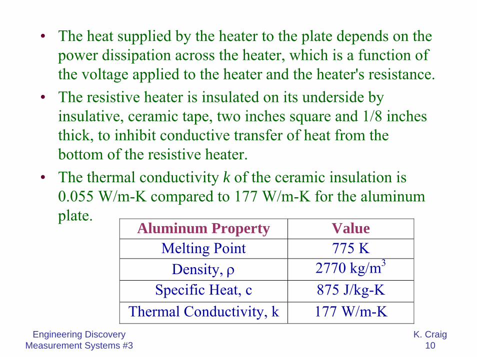
• The heat supplied by the heater to the plate depends on the power dissipation across the heater, which is a function of the voltage applied to the heater and the heater's resistance.
• The resistive heater is insulated on its underside by insulative, ceramic tape, two inches square and 1/8 inches thick, to inhibit conductive transfer of heat from the bottom of the resistive heater.
• The thermal conductivity k of the ceramic insulation is 0.055 W/m-K compared to 177 W/m-K for the aluminum plate.
Aluminum Property Value Melting Point 775 K
Density, ρ 2770 kg/m3 Specific Heat, c 875 J/kg-K
Thermal Conductivity, k 177 W/m-K
Engineering DiscoveryMeasurement Systems #3
K. Craig11
• The top of the thin, heated, aluminum plate is exposed to ambient air.
• Attached to the center of the heated plate is a temperature sensor whose electrical properties vary with the temperature of the surface to which it is bonded.
Engineering DiscoveryMeasurement Systems #3
K. Craig12
• Analog Devices 590 Temperature Sensor
Specification Value Rated Temperature Range -55° C to 150° C
Power Supply (min) 4 volts Power Supply (max) 30 volts
Nominal Output Current @ 298.2 K 298.2 µA Temperature Coefficient 1 µA/K
Calibration Error ± 2.5° C Maximum Forward Voltage 44 volts Maximum Reverse Voltage -20 volts Case Breakdown Voltage ± 200 volts
Engineering DiscoveryMeasurement Systems #3
K. Craig13
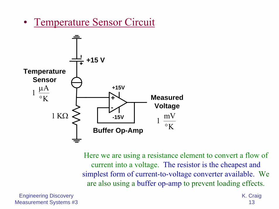
• Temperature Sensor Circuit
+15V
-15V-+
+15 VTemperature
SensorA1 Kµ°
1 KΩ
Buffer Op-Amp
Measured Voltage
mV1 K°
Here we are using a resistance element to convert a flow of current into a voltage. The resistor is the cheapest and
simplest form of current-to-voltage converter available. We are also using a buffer op-amp to prevent loading effects.
Engineering DiscoveryMeasurement Systems #3
K. Craig14
• Physical Model Simplifying Assumptions– Temperature of the plate is uniform– No heat loss through the sides of the plate– Thermal conductivity of the plate is constant– Heat loss due to radiation is negligible compared to
convective heat loss from the plate– Convection coefficient is constant and is evaluated at
the operating temperature of the plate– Heat loss through the insulative layer is negligible– Sensor dynamics are negligible– Ambient air temperature is unaffected by the heat flux
from the plate– Resistive heater is an ideal heat-flow source
Engineering DiscoveryMeasurement Systems #3
K. Craig15
Ambient air
Thin Aluminum Plate
q co
nvec
tion
Heat input qheater
Thin-Film Resistive Heater
Sensor
Ceramic Insulation
Physical Model
Input:Voltage supplied to resistive heater
Output:Plate temperature as measured by sensor on top of plate
Engineering DiscoveryMeasurement Systems #3
K. Craig16
• Electrical Analog
C Ri i ide ei Cdt R
deRC e Ridt
= +
= +
+ =
Kirchhoff’s Current Law
Engineering DiscoveryMeasurement Systems #3
K. Craig17
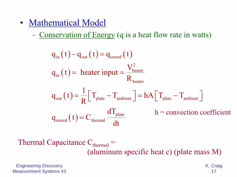
• Mathematical Model– Conservation of Energy (q is a heat flow rate in watts)
( ) ( ) ( )
( )
( )
( )
in out stored
2heater
inheater
out plate ambient plate ambient
platestored thermal
q t q t q t
Vq t heater inputR
1q t T T hA T TR
dTq t C
dt
− =
= =
⎡ ⎤ ⎡ ⎤= − = −⎣ ⎦ ⎣ ⎦
=h = convection coefficient
Thermal Capacitance Cthermal =(aluminum specific heat c) (plate mass M)
Engineering DiscoveryMeasurement Systems #3
K. Craig18
– Combine terms:
– Parameter Values:• Thermal Capacitance Cthermal = Mc = 4.96 J/K• Free Convection h = 5 to 25 W/m2K; choose h = 15
( ) ( ) ( )
( ) ( )
in out stored
2plateheater
plate ambient thermalheater
2plate heater
thermal plate ambientheater
2platethermal heater
plate ambientheater
q t q t q tdTV hA T T C
R dtdT VC hA T hA T
dt RdTC V1T T
hA dt hA R
− =
⎡ ⎤− − =⎣ ⎦
+ = +
⎛ ⎞ ⎡ ⎤+ = +⎜ ⎟ ⎢ ⎥⎣ ⎦⎝ ⎠
Engineering DiscoveryMeasurement Systems #3
K. Craig19
• Mathematical Analysis– How do we solve this differential equation?
– We use a numerical approximation and Excel:
2platethermal heater
plate ambientheater
platethermal plate in ambient
dTC V1T ThA dt hA R
dTRC T Rq T
dt
⎛ ⎞ ⎡ ⎤+ = +⎜ ⎟ ⎢ ⎥⎣ ⎦⎝ ⎠
+ = +
( )
platethermal plate in ambient
platethermal plate in ambient
plate in ambient platethermal
dTRC T Rq T
dtT
RC T Rq Tt1T Rq T T t
RC
+ = +
∆+ = +
∆⎡ ⎤
∆ = + − ∆⎢ ⎥⎣ ⎦
Engineering DiscoveryMeasurement Systems #3
K. Craig20
• Algorithm for Solving this Equation– Step 1: Initialize Variables
( )
( )
( )
thermal22
heaterin
heater
end
plate initial
1 1RhA (15) 0.00258
C 4.96
15VqR 185
t 0t 5 650
t 0.1 10
T 0 C above ambient temperature
= =
=
= =
== τ ≈
∆ < τ ≈
=
τ = RCthermal = 128 s
How did I know this?Is this small enough?
Engineering DiscoveryMeasurement Systems #3
K. Craig21
– Step 2: Increment time and stop when done
– Step 3: Compute qin(t). In this case, it is a constant.– Step 4: Solve
– Step 5: Determine new Tplate
– Step 6: Go back to Step 2
• Now Let’s Solve This in EXCEL and Graph the results!!!
end
t t tIf t t then stop= + ∆=
( )plate in platethermal
1T Rq T tRC⎡ ⎤
∆ = − ∆⎢ ⎥⎣ ⎦
( ) ( )plate plate platenew oldT T T= + ∆
Engineering DiscoveryMeasurement Systems #3
K. Craig22
• Engineers are well known for their ability to plot many curves of experimental data and to extract all sorts of significant facts from these curves.
• The better one understands the physical phenomena involved in a certain experiment, the better is one able to extract a wide variety of information from graphical displays of experimental data.
• Understand The Physical Processes Behind The Data!• When data may be approximated by a straight line, the analytical
relation is easy to obtain; but when almost any other functionalvariation (e.g., exponential, polynomial, complex logarithmic) is present, difficulties are usually encountered.
• It is convenient to try to plot data in such a form that a straight line will be obtained for certain types of functional relationships.
Engineering DiscoveryMeasurement Systems #3
K. Craig23
• The general form of our differential equation is:
• By separation of variables and integration, as shown in class, the response to a step input Kqis is:
• How can we plot this as a straight line?
oo i
dq q Kqdt
τ + =
t
0 isq Kq 1 e−τ
⎛ ⎞= −⎜ ⎟
⎝ ⎠
t
o ist
o
ist
o
is
q Kq (1 e )
q 1 eKq
q1 eKq
−τ
−τ
−τ
= −
= −
− =
tis o
is
tis
is o
Kq q eKq
Kq eKq q
−τ
τ
−=
=−
( ) ( )is
is o
log eKq tlog log e tKq q
⎛ ⎞ ⎡ ⎤= =⎜ ⎟ ⎢ ⎥− τ τ⎣ ⎦⎝ ⎠
• Straight-Line Graph
is
is o
KqlogKq q
⎛ ⎞⎜ ⎟−⎝ ⎠
time
( )log eslope =
τ
Engineering DiscoveryMeasurement Systems #3
K. Craig24
Engineering DiscoveryMeasurement Systems #3
K. Craig25
Voltage Sources & Meters:Ideal and Real
• Ideal Voltage Source– Supplies the intended voltage to the circuit no matter how
much current (and thus power) this might require– Can supply infinite current– Zero output impedance
• Real sources have terminal characteristics that are somewhat different from the ideal cases.
• However, the terminal characteristics of the real sources can be modeled using ideal sources with their associated input and output resistances.
Engineering DiscoveryMeasurement Systems #3
K. Craig26
• Real Voltage Source– Modeled as an ideal voltage source in series with a
resistance called the output impedance of the device.– When a load is attached to the source and current flows,
the output voltage Vout will be different from the ideal voltage source Vs due to voltage division.
– The output impedance of most voltage sources is usually very small (fraction of an ohm).
– For most applications, the output impedance is small enough to be neglected. However, the output impedance can be important when driving a circuit with small resistance because the impedance adds to the resistance of the circuit.
Engineering DiscoveryMeasurement Systems #3
K. Craig27
• Ideal Voltmeter– Infinite input impedance– Draws no current
• Real Voltmeter– Can be modeled as an ideal voltmeter in parallel with an
input impedance.– The input impedance is usually very large (1 to 10 MΩ).– However, this resistance must be considered when
making a voltage measurement across a circuit branch with large resistance since the parallel combination of the meter input impedance and the circuit branch would result in significant error in the measured value.
Engineering DiscoveryMeasurement Systems #3
K. Craig28
Rout
++
-- Ideal Voltage
Source
OutputImpedance
Vs Real VoltageSource
Vout
Engineering DiscoveryMeasurement Systems #3
K. Craig29
IdealVoltmeter
InputImpedance
Rin
RealVoltmeter
+
-
Vin
Engineering DiscoveryMeasurement Systems #3
K. Craig30
The Operational Amplifier
• Op-Amps are possibly the most versatile linear integrated circuits used in analog electronics.
• The Op-Amp is not strictly an element; it contains elements, such as resistors and transistors. However, it is a basic building block, just like R, L, and C.
• We treat this complex circuit as a black box!– Do we know all about the internal details? No!– Do we know how to use it and interface it with other
electronic components? Yes, we must!
Engineering DiscoveryMeasurement Systems #3
K. Craig31
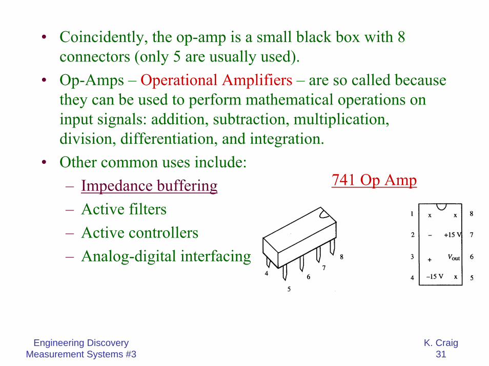
• Coincidently, the op-amp is a small black box with 8 connectors (only 5 are usually used).
• Op-Amps – Operational Amplifiers – are so called because they can be used to perform mathematical operations on input signals: addition, subtraction, multiplication, division, differentiation, and integration.
• Other common uses include:– Impedance buffering– Active filters– Active controllers– Analog-digital interfacing
741 Op Amp
Engineering DiscoveryMeasurement Systems #3
K. Craig32
• The op-amp has two inputs, an inverting input (-) and a non-inverting input (+), and one output. The output goes positive when the non-inverting input (+) goes more positive than the inverting (-) input, and vice versa. The symbols + and – do not mean that that you have to keep one positive with respect to the other; they tell you the relative phase of the output.
OutputInverting
Input+V
-V
-
+Non-Inverting
Input
A fraction of a millivolt between the input
terminals will swing the output over its full
range.
Engineering DiscoveryMeasurement Systems #3
K. Craig33
• Formal Definition of an Op-Amp:– dc-coupled: the op amp can be used with ac and dc
input voltages– differential voltage amplifier: the op amp has two
inputs– single-ended low-resistance output: the op amp has one
output whose voltage is measured with respect to ground.
– very high input resistance– very high voltage gain: op amp is a good voltage
amplifierVout
V2+V
-V
-
+V1
Vin = V1 - V25 6outopen loop
in
V A 10 10V
= ≈ −
Engineering DiscoveryMeasurement Systems #3
K. Craig34
• Since operational amplifiers have enormous and unpredictable voltage gain (106 or so), they are never used without negative feedback.
• Negative feedback is the process of coupling the output back in such a way as to cancel some of the input. This does lower the amplifier’s gain, but in exchange it also improves other op-amp characteristics, such as:– Freedom from distortion and nonlinearity– Flatness of frequency response or conformity to some
desired frequency response– Stability and Predictability– Insensitivity to variation in open-loop gain Aol
Engineering DiscoveryMeasurement Systems #3
K. Craig35
• As more negative feedback is used, the resultant amplifier characteristics become less dependent on the characteristics of the open-loop (no feedback) amplifier and finally depend only on the properties of the feedback network itself. For example:
Vout
Vin
RF
Rin
+V
-V
-
+
F
in
Fout in
in
RGainR
RV VR
=
= −
Basic Inverting Op-Amp
Engineering DiscoveryMeasurement Systems #3
K. Craig36
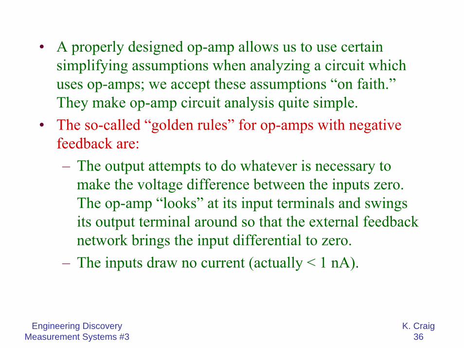
• A properly designed op-amp allows us to use certain simplifying assumptions when analyzing a circuit which uses op-amps; we accept these assumptions “on faith.”They make op-amp circuit analysis quite simple.
• The so-called “golden rules” for op-amps with negative feedback are:– The output attempts to do whatever is necessary to
make the voltage difference between the inputs zero. The op-amp “looks” at its input terminals and swings its output terminal around so that the external feedback network brings the input differential to zero.
– The inputs draw no current (actually < 1 nA).
Engineering DiscoveryMeasurement Systems #3
K. Craig37
• Basic Op-Amp Cautions– In all op-amp circuits, the “golden rules” will be
obeyed only if the op-amp is in the active region, i.e., inputs and outputs are not saturated at one of the supply voltages. Note that the op-amp output cannot swing beyond the supply voltages. Typically it can swing only to within 2V of the supplies.
– The feedback must be arranged so that it is negative; you must not mix the inverting and non-inverting inputs.
– There must always be feedback at DC in the op-amp circuit. Otherwise, the op-amp is guaranteed to go into saturation.
Engineering DiscoveryMeasurement Systems #3
K. Craig38
– Many op-amps have a relatively small maximum differential input voltage limit. The maximum voltage difference between the inverting and non-inverting inputs might be limited to as little as 5 volts in either polarity. Breaking this rule will cause large currents to flow, with degradation and destruction of the op-amp.
– Note that even though op-amps themselves have a high input impedance and a low output impedance, the input and output impedances of the op-amp circuits you will design are not the same as that of the op-amp.
Engineering DiscoveryMeasurement Systems #3
K. Craig39
• Non-Inverting and Unity-Gain Buffer Op-Amps
out 2
in 1
e R1e R
= +
eoutein
R2R1
+V
-V-
+
2
1
R 0R
→→∞
eoutein
+V
-V-
+
out
in
e 1e
=
Unity-Gain, Buffer Op-AmpNon-Inverting Op-Amp
Engineering DiscoveryMeasurement Systems #3
K. Craig40
• Inverting Op-Amp
out 2
in 1
e Re R
= −
1 23
1 2
R RRR R
=+
eout
ein
R2
R1
+V
-V
-
+
R3
Engineering DiscoveryMeasurement Systems #3
K. Craig41
• Summing Op-Amp
3 3out 1 2
1 2
R Re e eR R⎡ ⎤
= − +⎢ ⎥⎣ ⎦
eoute1
R3
R2
+V
-V
-
+
e2
R1
R4
Engineering DiscoveryMeasurement Systems #3
K. Craig42
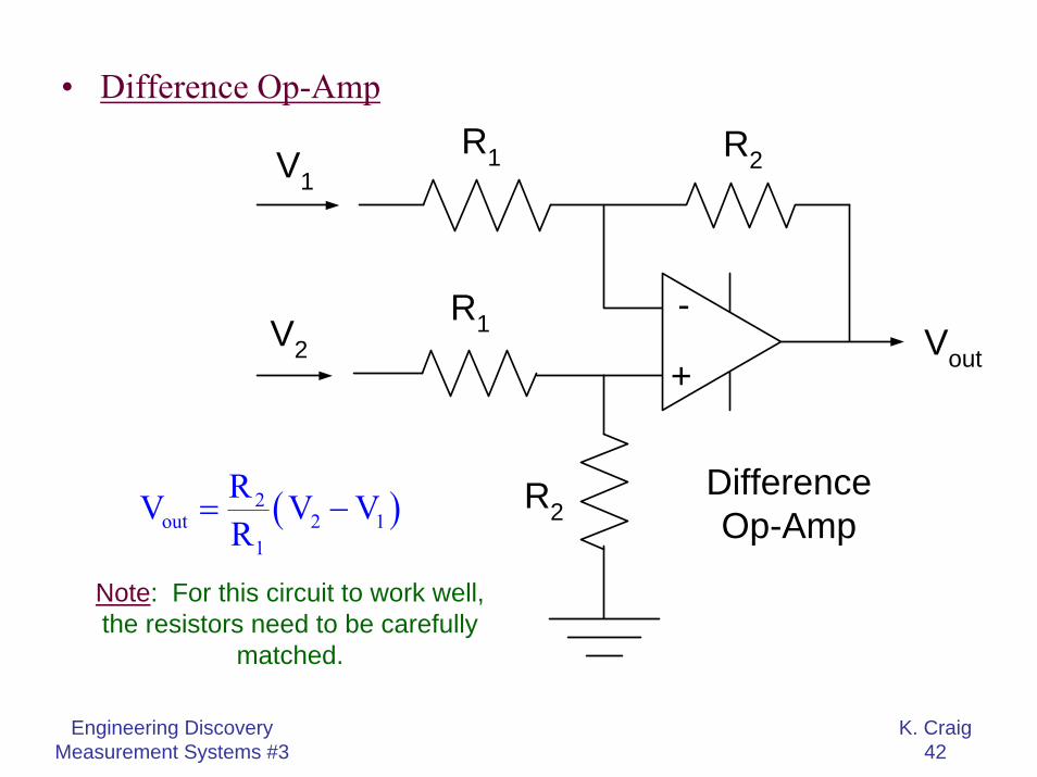
• Difference Op-Amp
( )2out 2 1
1
RV V VR
= −
Note: For this circuit to work well, the resistors need to be carefully