Work ing PaPer Ser ieSno 1646 / March 2014

Modeling eMergenceof the interbank netWorkS

Grzegorz Hałaj and Christoffer Kok

In 2014 all ECB publications

feature a motif taken from

the €20 banknote.

note: This Working Paper should not be reported as representing the views of the European Central Bank (ECB). The views expressed are those of the authors and do not necessarily reflect those of the ECB.

MacroPrUdential reSearch netWork

© European Central Bank, 2014

Address Kaiserstrasse 29, 60311 Frankfurt am Main, GermanyPostal address Postfach 16 03 19, 60066 Frankfurt am Main, GermanyTelephone +49 69 1344 0Internet http://www.ecb.europa.euFax +49 69 1344 6000

All rights reserved.

ISSN 1725-2806 (online)EU Catalogue No QB-AR-14-020-EN-N (online)

Any reproduction, publication and reprint in the form of a different publication, whether printed or produced electronically, in whole or in part, is permitted only with the explicit written authorisation of the ECB or the authors.This paper can be downloaded without charge from http://www.ecb.europa.eu or from the Social Science Research Network electronic library at http://ssrn.com/abstract_id=2397106.Information on all of the papers published in the ECB Working Paper Series can be found on the ECB’s website, http://www.ecb.europa.eu/pub/scientific/wps/date/html/index.en.html

Macroprudential Research NetworkThis paper presents research conducted within the Macroprudential Research Network (MaRs). The network is composed of economists from the European System of Central Banks (ESCB), i.e. the national central banks of the 27 European Union (EU) Member States and the European Central Bank. The objective of MaRs is to develop core conceptual frameworks, models and/or tools supporting macro-prudential supervision in the EU. The research is carried out in three work streams: 1) Macro-financial models linking financial stability and the performance of the economy; 2) Early warning systems and systemic risk indicators; 3) Assessing contagion risks.MaRs is chaired by Philipp Hartmann (ECB). Paolo Angelini (Banca d’Italia), Laurent Clerc (Banque de France), Carsten Detken (ECB), Simone Manganelli (ECB) and Katerina Šmídková (Czech National Bank) are workstream coordinators. Javier Suarez (Center for Monetary and Financial Studies) and Hans Degryse (Katholieke Universiteit Leuven and Tilburg University) act as external consultants. Fiorella De Fiore (ECB) and Kalin Nikolov (ECB) share responsibility for the MaRs Secretariat.The refereeing process of this paper has been coordinated by a team composed of Gerhard Rünstler, Kalin Nikolov and Bernd Schwaab (all ECB). The paper is released in order to make the research of MaRs generally available, in preliminary form, to encourage comments and suggestions prior to final publication. The views expressed in the paper are the ones of the author(s) and do not necessarily reflect those of the ECB or of the ESCB.

AcknowledgementsThe authors are indebted to J. Henry, I. Alves and other participants of an internal ECB seminar who provided valuable comments and to C. Minoiu and VS Subrahmanian who discussed the paper during INET conference in Ancona.

Grzegorz Hałaj (corresponding author)European Central Bank; e-mail: grzegorz.halaj@ecb.europa.eu

Christoffer KokEuropean Central Bank

Abstract

Interbank contagion has become a buzzword in the aftermath of the financial crisisthat led to a series of shocks to the interbank market and to periods of pronounced marketdisruptions. However, little is known about how interbank networks are formed and abouttheir sensitivity to changes in key bank parameters (for example, induced by common ex-ogenous shocks or by regulatory initiatives). This paper aims to shed light on these issuesby modelling endogenously the formation of interbank networks, which in turn allows forchecking the sensitivity of interbank network structures and hence their underlying con-tagion risk to changes in market-driven parameters as well as to changes in regulatorymeasures such as large exposures limits. The sequential network formation mechanismpresented in the paper is based on a portfolio optimisation model whereby banks allocatetheir interbank exposures while balancing the return and risk of counterparty default riskand the placements are accepted taking into account funding diversification benefits. Themodel offers some interesting insights into how key parameters may affect interbank net-work structures and can be a valuable tool for analysing the impact of various regulatorypolicy measures relating to banks’ incentives to operate in the interbank market.

Keywords:interbank network, financial contagion, counterparty risk, financial regulationJEL Codes: G21, C63, C78

1

Non-technical summary

A key characteristic about the recent financial crisis was the potential for shocks hitting spe-cific financial institutions to spread (quickly) across the entire system – the Lehman Brothersdefault in the Autumn 2008 being the most prominent event. These experiences have thereforefostered a wealth of studies on financial contagion, many of which apply network theory, tobetter understand the inherent riskiness of the financial system via the interconnectedness offinancial institutions. A key finding in the literature is that contagion risks in for examplethe interbank market is very much determined by the structure of the network through whichbanks are interconnected. In other words, the scope for contagious losses following an id-iosyncratic or system-wide shock depends on the number of connections and the centrality ofaffected institutions in the network. However, little is known about how financial networks areformed and about their sensitivity to changes in key bank parameters (for example, inducedby common exogenous shocks or by regulatory initiatives).

Focusing on interbank market contagion, this study adds to this literature by modellingendogenously the formation of interbank networks, which in turn allows for checking thesensitivity of interbank network structures and hence their underlying contagion risk to changesin market-driven parameters as well as to changes in regulatory measures. Especially the latterdimension is of relevance from a macro-prudential policy perspective. An in-depth knowledgeabout how network structures are affected by specific macro-prudential policy measures iscrucial for assessing the effectiveness and relevance of such policies. In this paper, we focuson a macro-prudential (and micro-prudential) policy instrument that is embedded in the newBasel standards and are directly related to interbank interconnectedness; namely, the largeexposures limits. However, the modelling approach could also be applied to evaluate othertypes of prudential policy measures, for instance risk weights to other financial institutions.

The methodology proposed in this paper for modelling endogenous network formationis related both to so-called agent-based modelling as well as to game theoretical concepts.Specifically, the sequential network formation mechanism presented in the paper is based on aportfolio optimisation model whereby banks allocate their interbank exposures while balancingthe return and risk related to levels and volatility of market interest rates and counterpartydefault risk and the placements are accepted taking into account funding diversification ben-efits. More precisely, the interbank network is an outcome of a sequential game played bybanks trying to invest on the interbank market and to borrow interbank funding. We take asample of 80 large EU banks and based on their balance sheet composition assume that theyoptimise their interbank assets taking into account risk and regulatory constraints as well asthe demand for the interbank funding. This optimisation process results in a preferred inter-bank portfolio allocation for each bank in the system. For what concerns the funding side,banks define their most acceptable structure of funding sources with the objective of limitingrefinancing (rollover) risk. Banks meet in a bargaining game in which the supply and demandfor interbank lending is determined by allowing banks to marginally deviate from their optimalinterbank allocations and the prices they offer on those. In order to account for the quite com-plex aspects of the interbank market formation we propose a sequential optimisation process,each step of which consisting of four distinctive rounds. The sequential optimisation processis repeated in an iterative manner until a satisfactory level of convergence (i.e. full allocationof interbank assets) is achieved.

The model offers some interesting insights into key parameters affecting interbank network

2

structures and can be a valuable tool for analysing the impact of various regulatory policymeasures relating to banks’ incentives to operate in the interbank market.

We find that the endogenous network model produces realistic, and complex, networkconfigurations. Our approach allows for assessing the derived interbank structures againstrelevant network benchmarks and for verifying their sensitivity to key driving parameters, suchas correlation (Q), loss given default (λ), investment risk aversion (κ), funding risk aversion(κF ), interbank interest rate elasticity (α) and capital allocated to the interbank portfolios(eI). In general, we find that interbank asset correlation appears to have a sizable impact onthe structure of the endogenous network formation whereby high correlation translates into lowdiversification potential which tends to lead to a concentration of exposures in a few banks. Ingeneral, the interbank network structures derived by the model vary in a limited way to changesin key parameters and the variability that is observed tends to have intuitive explanations. Forinstance, increasing investment risk aversion leads on average to the decrease in the number oflinkages. The structure of the endogenously derived interbank network (the number of linkagesbetween banks) is also found to be sensitive to deposit interest rate elasticity and the level ofallocated capital to the interbank portfolios.

In terms of policy experiments, we examine the impact of the network structures and thecontagion risks related to internal risk limit systems and regulatory instruments aimed at limit-ing banks’ risk to counterparty exposures, such as the Credit Valuation Adjustment charge onthe capital allocated to the interbank asset portfolios and the regulatory large exposure limitsalready embedded in current regulatory frameworks. The EU directive on prudential supervi-sion from June 2013 introduces special risk weights for exposures to financial institutions as anew macro-prudential tool and the concept of Credit Valuation Adjustment can be applied totest performance of the risk sensitive risk weights for the exposures to financial institutions.Apart from the evaluation of relevant regulatory instruments, the endogenous network modelcan also be employed in macro-prudential analysis in a broader sense. Namely, it can improvethe assessment of the impact of the materialisation of systemic risks on the banking sectorwhile taking into account the dynamic network formation resulting from changes in key realeconomic and financial variables. In particular, as an adverse shock to the economy wouldtypically result in the deterioration of some counterparties’ creditworthiness (e.g. as reflectedin banks’ CDS spreads) and hence affect the optimal allocation of interbank assets and liabil-ities. In other words, a given adverse scenario is likely to result in a rewiring of linkages inthe interbank market and hence to also affect the interbank contagion risks that ultimatelymay result from such adverse shocks. Our findings suggest that in particular the setting oflarge exposure limits can have a pronounced impact of the level of contagion risks embeddedin the interbank market, whereas the effects from the CVA appear more limited and ambigu-ous. All in all, while the reported results obviously hinges on the specific characteristics ofthe banks included in the network system and on the specific adverse scenarios considered,the overriding conclusion from these policy experiments is that macro-prudential policies canmake a significant difference through their impact on the network formation and ultimatelyon the risk of interbank contagion to adverse shocks. From this perspective, the modelling ap-proach presented in this paper can be employed for conducting impact assessments of selectedmacro-prudential policy instruments and in this way help inform the calibration of such tools.

3

1 Introduction

The interbank market was one of the main victims of the financial crisis erupting in 2007.The crisis led to a general loss of trust among market participants and resulted in severe in-terbank market disruptions. Moreover, failures of some key market players triggered concernsabout risks of interbank contagion whereby even small initial shocks could have potentiallydetrimental effects on the overall system. As a results of these concerns, and also reflecting abroader aim of making the financial sector more resilient, in recent years financial regulatorshave introduced various measures that aim at mitigating (and better reflecting) the risks inher-ent through the bilateral links between banks in the interbank network. These internationalreform initiatives range inter alia from limits on large counterparty exposures, higher capitalrequirements on counterparty exposures related to the OTC derivatives and requirements tosettle standardised OTC derivatives contracts via central counterparty clearing (CCP) houses.While it seems plausible that these initiatives should help alleviate contagion risks in the in-terbank market, there is still only little research aiming to quantify and understand the effectsof these reforms on network structures and the contagion risk that might emerge from thesestructures.

Against this background, this paper aims to help fill this gap in the literature by improvingour understanding of risks stemming from bank interconnectedness and how specific regulatorymeasures can affect interbank network structures and hence contagion risk. When trying toassess how different policy measures are likely to impact on interbank network formation, it willbe crucial to also take into account how banks could be expected to react to these measures.For this reason, the starting point of the analysis presented in this paper is to establish a settingwhereby network structures emerge on the basis of banks’ endogenous reactions to changes inthe environment affecting their optimal asset and liability mix (and hence also their decisionto lend in the interbank market).

For this purpose, the paper presents a model to derive interbank networks that are deter-mined by certain characteristics of banks’ balance sheets, the structure of which is assumedto be an outcome of banks’ risk-adjusted return optimisation of their assets and liabilities.The model of bank balance sheet optimisation is combined with the random network genera-tion technique presented in (Ha laj and Kok, 2013b). This allows us to study the endogenousnetwork formation based on optimising bank behaviour.

The model can thus help to understand the foundations of topology of the interbanknetwork. It furthermore provides a tool for analysing the sensitivity of the interbank structuresto the heterogeneity of banks (in terms of size of balance sheet, capital position, generalprofitability of non-interbank assets, counterparty credit risk) and to changes of market andbank-specific risk parameters. Such parameter changes could for example be due to regulatorypolicy actions (for example, pertaining to capital buffers as well as the size and diversity ofinterbank exposures) aiming at mitigating systemic risk within the interbank system. Theframework developed in this paper can therefore be used to conduct a normative analysis ofmacro and micro-prudential policies geared towards more resilient interbank market structures.

The paper is related to research on network formation which was only recently pursuedin finance. Understanding the emergence process of the interbank networks can be critical tocontrol and mitigate these risks. Endogenous networks (and their dynamics) are a difficultproblem since the behaviour of the agents (banks in particular) is very complex. In other areasof social studies, the network formation was addressed by means of network game techniques

4

(Jackson and Wolinsky, 1996). In financial networks, researchers also applied recently gametheoretical tools (Acemoglu et al., 2013; Cohen-Cole et al., 2011; Babus and Kondor, 2013;Bluhm et al., 2013; Gofman, 2013) or portfolio optimisation (Georg, 2011).1 For instance,Acemoglu et al. (2013) shows that the equilibrium networks generated via a game on a spaceof interbank lending contracts posted by banks can be socially inefficient since financial agents“do not internalize the consequences of their actions on the rest of the network”.2 In Cohen-Cole et al. (2011) banks respond optimally to shocks to incentives to lend. Bluhm et al. (2013)approach to modelling endogenous interbank market is closely related to ours. However, themain distinctions from our approach are: risk neutrality of banks, riskiness of the interbankassets introduced to the model only via capital constraints and not including funding riskas having a potential impact on the interbank structure. Castiglionesi and Lavarro (2011)presented a model with endogenous network formation in a setting with micro-founded bankingbehaviour.3 These advances notwithstanding, owing to the complexity of the equilibrium-basedstudies of network formation, agent-based modeling of financial networks is one promisingavenue that can be followed (Markose, 2012; Grasselli, 2013).

This paper adds to this strand of the literature by taking a model of portfolio optimisingbanks to a firm-level data set of European banks, which in turn allows us to study withinan endogenous network setting the impact of plausible internal limit systems based on creditvaluation adjustments (CVA) accounting for counterparty credit risk (Deloitte and Partners,2013) and various regulatory policy measures on interbank contagion risk. Apart from theasset-liability optimising behaviour that we impose on the agents (i.e. the banks), our net-work formation model also incorporates sequential game theoretical elements. If the portfoliooptimisation of interbank investment and interbank funding does not lead to a full matchingof interbank assets and liabilities, banks will engage in a bargaining game while taking intoaccount deviations in their optimal levels of diversification of investment and funding risks(see e.g. Rochet and Tirole (1996)).4 The sequence of portfolio optimisation and matchinggames is repeated until the full allocation of interbank assets at the aggregate level has beenreached. The outlined mechanism is also related to studies on matching in the loan market (seee.g. (Fox, 2010; Chen and Song, 2013)). Furthermore, to further reduce mismatches betweenbanks’ funding needs and the available interbank credit emerging from the portfolio optimis-ing choices, we introduce an interbank loan pricing mechanism that is related to models ofmoney market price formation (see e.g. (Hamilton, 1998; Ewerhart et al., 2004; Eisenschmidtand Tapking, 2009)). Importantly, as argued by ad A. Kovner and Schoar (2011) such pricingmechanisms can be expected to be more sensitive to borrower characteristics (and risks) duringperiods of stress. The model presented here would be able to account for such effects.

The paper is structured as follows: Section 2 presents the model of network formation underoptimising bank behaviour. In Section 3 some topology results from the network simulationsare presented, while in Section 4 it is illustrated how the model can be applied for studyingvarious macro-prudential policy measures. Section 5 concludes.

1Some earlier contributions incorporating multi-agent network models, albeit with fixed network and staticbalance sheet assumptions, include (Iori et al., 2006; Nier et al., 2007).

2See also Gai and Kariv (2003) for an earlier contribution.3Other studies in this direction include (Babus, 2011; Castiglionesi and Wagner, 2013).4While not explicitly taken into account in this paper, this is related to the literature on interbank lending

where due to asymmetric information banks are not able to perfectly monitor their peers. Such informationasymmetries may be reinforced by adverse shocks as for example experienced during the recent financial crisis,see Heider et al. (2009).

5

Figure 1: The sequential four round procedure of the interbank formation

2) OPTIMISATIONPreferred funding

structure

1) OPTIMISATIONPreferred asset

structure 4) PRICE ADJUSTMENTOffered IB interest rates

3) BILATERAL GAMESBargaining game

STEPS Repeateduntil all IB assetsare allocated

Unallocated IB assets and liabilities

NEW PLACEMENTSPart of unallocated IB assetsplaced in banks as deposits

creating IB linkages

4 ROUNDS

REPEATED

STEPS

Next step

Full allocation IB Network Completed

Partial allocation

INITIAL PARAMETERSAggregate IB lending / borrowing, capital, Risk Weighted Assets,

CDS spreads, market interest ratesConstraints: allocated capital, Large Exposure limits, Credit Valuation Adjustment

2 Model

2.1 Outline

The interbank network described in this paper is an outcome of a sequential game playedby banks trying to invest on the interbank market and to borrow interbank funding. Banksoptimise their interbank assets taking into account risk and regulatory constraints as well asthe demand for the interbank funding and propose their preferred portfolio allocation. Forwhat concerns the funding side banks define their most acceptable structure of funding sourceswith the objective to limit refinancing (rollover) risk. Banks meet in a bargaining game inwhich the supply and demand for interbank lending is determined. In order to account for thequite complex aspects of the interbank market formation we propose a sequential optimisationprocess, each step of which consisting of four distinctive rounds (see the block scheme in figure2.1).

There are three main general assumptions of the model:

1. Banks know their aggregate interbank lending and borrowing as well as those of otherbanks in the system. It is a public information for all the banks in the sample.

2. Banks optimise the structure of their interbank assets, i.e. their allocation across coun-terparties.

3. Banks prefer diversified funding sources in terms of rollover risk (i.e. liquidity risk relatedto the replacement of the maturing interbank deposits).

This first, rather strong assumption has its motivation in the stable over time fraction of

6

interbank assets to total liabilities, confirmed empirically in a sample of 90 largest EU banks.5

In theory, part of that assets and liabilities, in particular with the shortest maturities, can bevolatile since it reacts to volatile banks’ liquidity needs. However, the interbank investmentportfolio and interbank funding portfolio may be much more stable since their volumes shouldresult from a general asset-liability planning within the ALM process defining, inter alia atarget for product mix of assets and funding sources and income parameters. The targetsare managed by a system of limits on exposures or pricing offered by various business linestaking a holistic perspective on the balance sheet and taking into account market conditions,general goals set by executive board and strategies set by the ALCO. We do not model theoutcomes of a preceding ALM process and treat the volumes of interbank assets and liabilitiesas given and deterministic. The uncertainty in the model stems from interest risk, counterpartycredit risk and funding roll-over risk. The second assumption follows the standard portfoliochoice theory. Optimisation is constraint by regulatory liquidity and capital rules and therelationship lending; banks are assumed to optimise their portfolio in a set of counterpartieswith whom they built up relationship lending. The third assumption refers to the set of banks’counterparties. Based on lending relationship, each bank has a subgroup of partners on theinterbank market with whom it is likely to trade. It is reasonable to assume that banks try tominimise funding risk in their subgroups. Notably, there is some empirical evidence (Brauningand Fecht, 2012) that the relationship lending may impact pricing of interbank loans andconsequently also funding structure. All in all, the decision about the funding structure is afunction of diversification needs and build-up of relationship lending.

In the first round, banks specify the preferred allocation of interbank assets by maximisingthe risk-adjusted return from the interbank portfolio. Banks are assumed to be risk aversewhich follows the approach taken in capital management, whereby accepted levels of exposureare commonly managed via RAROC6 and RARORAC ALM indicators (Adam, 2008). Inthe traditional banking literature (Baltensperger, 1980; Boyd and Nicolo, 2005; Pelizzon andSchaefer, 2005) banks are assumed to take investment decisions under risk neutrality assump-tion.7 Risk impacts banks’ decisions via regulatory constraints. We follow an approach froma different strand of literature (Howard and Matheson, 1972; Danielsson et al., 2002; Cuocoand Liu, 2006) where decisions are risk sensitive. In fact, Baltensperger (1980) admits thatjoint modelling of loan or deposit volumes and diversification within these two portfolios canbe approach rather by utility maximisation (implying risk sensitive decisions) than expectedprofit maximisation.

In this optimisation process, each bank first draws a sample of banks according to a pre-defined probability that a bank is related to another bank. The probability map was developedby Ha laj and Kok (2013b) using the geographical breakdown of banks’ exposures disclosedduring the EBA 2011 capital exercise. Second, they make offers of interbank placements ata current market rate trying to maximise the return adjusted by investment risk taking intoaccount:

expected interest income;

risk related to interest rate volatility and potential default of counterparts, and correla-

5A standard deviation of quarterly ratios of interbank assets or interbank liabilities to total assets amountson average to 2.5%.

6Risk-Adjusted Return on Capital and Risk-Adjusted Return on Risk-Adjusted Capital7See also Elyasiani et al. (1995); Balasubramanyan and VanHoose (2013)

7

tion among risks;

internal risk limits for capital allocated to the interbank portfolio, based on the CreditValuation Adjustment (CVA) concept8 and regulatory constraints in form of the LargeExposure limits specifying the maximum size of an exposure in relation to the capitalbase;

exogenous volume of total interbank lending.

Notably, the structure rather then the aggregate volume of lending is optimised. The aggregateinterbank lending and borrowing of banks in the model is exogenous.

Obviously, the recipients of the interbank funding can have their own preferences regardingfunding sources. Therefore, in the second round of the model, after the individual banks’optimisation of interbank assets, banks calculate their optimal funding structure, choosingamong banks that offered funding in the first round. They decide about the preferred structurebased on the funding risk of the resulting interbank funding portfolios. There is a clearmotivation behind separating the optimisation process into interbank investment and fundingchoice. The model operates on two distinct types of portfolios: investment and funding. Assetand liability management process may give different priorities to management actions targetedat interbank assets and at interbank liabilities. For instance, banks may be more sensitive tothe risk in their interbank funding portfolios since they may constitute a sizeable part oftheir funding sources. The setup of the model gives flexibility to parameterise risk aversiondifferently for optimisation of interbank assets and interbank liabilities but in the applicationswe use a common value for the two risk aversion parameters.

The offers of interbank placements may diverge from the funding needs of the other side ofthe interbank market. In the third round we therefore assume that pairs of banks negotiate theultimate volume of the interbank deposit. We model these negotiations by means of a bargain-ing game in which banks may be more or less willing (or sensitive from an utility perspective)to deviate from their optimisation-based preferred asset-liability structures. Notably, also atthis round banks take into account their risk and budget constraints.

Since interbank asset and interbank funding optimisation followed by the game may notresult in full allocation of the predefined interbank assets and in satisfaction of all the interbankfunding needs the prices on the interbank market may be adjusted. In the fourth round bankswith an open funding gap are assumed to propose a new interest rate for the new interbankinvestors depending on the relative size of the gap to their total interbank funding needs.Implicitly, we do not model the role of the central bank which normally stands ready toprovide liquidity.

The four consecutive rounds are repeated with a new drawing of banks to be includedinto sub-samples of banks with which each bank prefers to trade. Consequently, each bankenlarges the group of banks considered to be their counterparties on the interbank market andproposes a new preferred structure of the interbank assets and liabilities for the unallocatedpart in the previous step. In this way, the interbank assets and liabilities are incrementallyallocated among banks.

8This CVA element is not to be mistaken with the CVA capital charge on changes in the credit spread ofcounterparties on OTC derivatives transactions. However, the line of calculation is similar. Some banks useCVA internally to render exposure limits sensitive to the counterparty risk in a consistent, model-based way(Deloitte and Partners, 2013).

8

Modelling the network formation process in sequential terms, is obviously somewhat stylisedas in reality banks are likely to conduct many of the steps described here in a simultaneousrather than sequential fashion. At the same time, the step-by-step approach is a convenientway of presenting the complex mechanisms that determine the formation of interbank linkages,which may realise in a very short time-span, even only several tick long.

The following subsections describe in details how the endogenous networks are derived.Some important notations used thereafter are introduced below.Notation: N stands for set 1, 2, . . . , N, ‘∗’ denotes entry-wise multiplication, i.e. [x1, . . . , xN ]∗[y1, . . . , yn] : = [x1y1, . . . , xNyN ], ‘>’ is transposition operator and – for matrix X – X·j de-notes jth column of X and Xi· denotes ith row of X, #C – number of elements in a set C, IAdenotes indicator function of a set A.

2.2 Banks

First, a description of banks’ balance sheet structures, interbank assets and liabilities in par-ticular, is warranted. It is supposed that there are N banks in the system. Each institutioni aims to invest ai volume of interbank assets and collect li of interbank liabilities. Thesepre-defined volumes are dependent on various exogenous parameters. For instance, individualbanks’ aggregate interbank lending and borrowing can be an outcome of asset and liabilitymodeling (ALM).9. The interest rates paid by interbank deposits depend on:

some reference market interest rates rm (e.g. the 3-month offered interbank rate incountry m),

a credit risk spread (si) reflecting the credit risk of a given bank i,

a liquidity premium qi referring to the general market liquidity conditions and bank i’saccess to the interbank market10,

Loss Given Default (LGD) related to the exposure, denoted λ.

The LGD is assumed to be equal for all banks and exposures and amounting to 40%. Wedo not model maturity structure of the interbank assets and liabilities in the current setting,i.e. all interbank assets and liabilities have the same maturity.

The credit spread si is translated into a bank-specific interest rate paid by bank i to itsinterbank creditors – ri. It is based on the notion of equivalence of the expected returns frominterbank investment to a specific bank and from investing into the reference rate rm,

rm + qi ≡ ripiλ+ (1− pi)ri, (1)

where pi denotes marginal probability of default on the interbank placement extended to banki and is calculated as

pi : = si/λ

Interest rate ri can be interpreted as a rate that realises the expected return of rm given thedefault risk captured by the spread si.

11 We use a very basic approximation of the default

9Georg (2011) or Ha laj (2013) developed frameworks based on the portfolio theory to optimise the structureof investments and funding sources that could be followed.

10We assume for simplicity that q ≡ 0 while indicating how liquidity can be captured in the framework.11Currency risk related to the cross-border lending between countries with different currencies is not addressed

in the model.

9

probability pi derived from the spread si but still we are able to gauge differences in defaultrisk among bank and the definition of pis is not key in developing the modelling frameworkfor endogenous interbank networks.

Moreover, the cost – or a return from the interbank placement perspective – is risky.The riskiness is described by a vector σ : = [σ1 . . . σN ]> of standard deviations of historical(computed) rates ri and correlation matrix Q of these rates calculated from equation 1 takinginto account time series of interbank rates and CDS spreads.12 The riskiness stems fromthe volatility of market rates and variability of default probabilities. Likewise, correlation isrelated to:

the common reference market rate for banks-debtors in one country or co-movement ofreference rates between countries which the cost of interbank funding is indexed to;

to the correlation of banks’ default risk.13

Banks are also characterised by several other parameters not related to the interbankmarket but important in our framework from the risk absorption capacity perspective.

capital ei; and capital allocated to the interbank exposures eIi (e.g. economic capitalbudgeted for treasury management of the liquidity desk);

risk weighted assets RWAi – similarly, RWAIi risk-weighted assets calculated for the

interbank exposures. This may depend on the composition of the portfolio, i.e. exposureto risk of different counterparts.

All the aforementioned balance sheet parameters are used in the following subsections to definebanks’ optimal investment and funding programs.

2.3 First round – optimisation of interbank assets

Each bank is assumed to construct its optimal composition of the interbank portfolio givenmarket parameters, risk tolerance, diversification needs (also of a regulatory nature) and capitalconstraints (risk constraints including the Credit Valuation Adjustments (CVA) introducedwithin Basel III).

2.3.1 Prerequisites

Let Lij denote an interbank placement of bank j in bank i. Bank risk aversion is measuredby κ ≥ 0. CVA is assumed to impact the economic capital and, consequently the potentialfor interbank lending.14 For simplicity, we assume that an interbank exposure of volumeLij requires γiLij to be deducted from capital eIj , for γi being bank specific CVA factor, toaccount for the market based assessment of the credit risk related with bank i. A possibleway to calculate CVA is presented in the appendix. The parameter γ can also be viewed

12Other measures can be applied, e.g. VaR-based, reflecting the tail risks or some multiples of standarddeviation (2-, 3-times standard deviation).

13Reason: banks operate on similar markets, have portfolios of clients whose credit quality depends on similarfactors, their capital base is similarly eroded by the deteriorating market conditions, etc.

14BCBS (2011) stipulates rules to account for the counterparty risk in the regulatory capital. From thatviewpoint and for consistency, eIi can also be treated as regulatory capital.

10

as a risk sensitive add-on to the risk weights applied to the interbank exposures. The laterinterpretation gives rise to the macro-prudential application of the CVA concept and it isillustrated in section 4.

Banks are assumed to trade most likely with banks with which they have an establishedcustomer relationship. This is proposed to be captured by banks’ geographical proximity aswell as the international profile of the bank. It is assumed that banks are more likely to tradewith each other if they operate on the same market. The probability map (P ) of interbanklinkages, introduced by Ha laj and Kok (2013b) and calculated based on the banks’ geographicalbreakdown of exposures, is used to sample banks with which a given bank intends to trade.The maturity is standard and common across the market and the rate is determined by thereference rate and the credit quality of the borrower (see identity 1).

2.3.2 Procedure

Since the formation of the interbank network is modelled in a sequential way, we set the initialvalues of banks’ assets and liabilities to be matched on the interbank market at the stepsk = 1, 2, 3... and of a structure of the interbank network, i.e. for k = 0

l0 = l,

a0 = a,

L0 = 0N×N

Vectors ak, lk denote banks’ aggregate interbank lending and borrowing which is still notallocated among banks before step k. A matrix Lk denotes the structure of linkages on theinterbank market created up to the step k of the algorithm. Additionally, for notationalconvenience we denote B0

j = ∅ the initial empty set of banks in which a given bank j intendsto invest.

At step k, bank j draws a sample of banks Bkj ⊂ N/j. More specifically, each counter-

party i of the bank j is accepted with probability Pij .15 Banks from the set Bk

j are assumed

to enlarge the set of investment opportunities of bank j, i.e. Bkj = Bk−1

j ∪Bkj . At step k, the

bank considers (optimally) extending interbank placements to banks Bkj .

Bank j is assumed to maximise the following risk-adjusted return form the interbankinvestment:

J(Lk1j , . . . , L

kNj) =

∑i|i 6=j

rki Lkij − κj(σ ∗ Lk

·j)>Q(σ ∗ Lk

·j), (2)

where r1 ≡ r and rates rk in steps k ≥ 2 of the endogenous network algorithm can varyaccording to adjustments related to the funding needs of banks that have problems withfinding enough interbank funding sources (see subsection 2.6). The vector of risk measuresσ was defined in section 2.2. The interest rates rk paid by the interbank deposits are thetransaction rates defined by equation 1 and the risk – both related to market interest rate riskand default risk – is captured by the covariance (σ ∗ Lk

·j)>Q(σ ∗ Lk

·j).

Given the drawn sample Bkj , the set of admissible strategies is

Akj : = y ∈ RN

+ |for all n 6∈ Bkj yn = 0

15It can be thought of as a trader of bank j calling they counterparties randomly but potentially with higherchance of selecting banks more closely related in trading with j.

11

subject to further constraints related to risk and regulations. Akj can be interpreted as set of

bank j’s actions allowing for investing only in the drawn subsample. Obviously, starting froma different seed the sampling may cover any configurations of banks which are allowed by theprobability map P .

The maximum value of the functional (2) always exists; however, it may not be unique. Thismay happen if there are banks with the same characteristics of return and risk. Theoreticallyis is highly unlikely, however in practice, we use peers’ parameters for banks with unavailableindividual data on interbank interest rates and credit default spreads. Having two identicalbanks with respect to return and risk parameters means that other market participants can beindifferent to which of them to lend. In our setting, only the size of banks and their customerrelationship P matter. Therefore, we calculate the theoretically optimal breakdown of theinterbank placements taking into account a random representative for a group of identicalbanks and then average out the results.

In the baseline setting of the endogenous networks we do not restrict the size of exposuresa bank is allowed to hold against another bank. However, in practice banks are constrainedby so-called “large exposure limits” (LE).16 To account for such regulations, we impose oneadditional condition:

each exposure should not exceed χ > 0 fraction of the total regulatory capital.

In the current EU Capital Requirements Directive χ is assumed to be equal to 0.25. Moreover,there is the additional requirement that the sum of all exposures that (individually) exceed10 per cent of the capital should not surpass 800 per cent of capital. The second requirementwould introduce a nonlinearity in the set of constraints in our model and we decide not toinclude it. However, the large exposure limit imposed on the individual interbank placementproves to be a more stringent constraint and its severity can be tuned and tested by shifting itsufficiently below 25%. All in all, our baseline setup of the model excludes the large exposurelimit constraints which are introduced for sensitivity analysis of the network structures.17

The maximisation of the functional (2) is subject to some feasibility and capital constraints.

1. budget constraint –∑

j|j 6=i Lkij = akj and Lk

jj = 0, where – just to remind – a0i is exoge-

nously determined;

2. counterpart’s size constraint – Lkij ≤ lki ;

3. capital constraint –∑

i|i 6=j ωi(Lkij + Lk

ij) ≤ eIj − γ · (Lk·j + Lk

·j) or equivalently∑i|i 6=j(ωi + γi)(L

kij + Lk

ij) ≤ eIj ;

4. (optionally) large exposure limit constraint – (Lkij + Lk

ij) ≤ χej .

Given the risk constraints on the one hand and the riskiness of the interbank lending on theother hand, it may not be possible for a bank i to place exactly aki interbank deposits in totalin step k. Therefore, the budget constraint may not be plausible – as a consequence the banki should consider lending less.18 We apply the following compromising iterative procedure.

16See Article 111 of Directive 2006/48/EC that introduces the limits.17More discussions of the LE impact on the structure of the interbank system can be found in Ha laj and Kok

(2013a).18In an extreme case, also the LE constraints may prove to be too severe. The system is not solvable if there

exists a pair (k, j) such that χ∑

j|j 6=k ej < lk, which means that bank k is not able to find the predefinedvolume lk of the interbank funding.

12

The bank is assumed to solve a problem with budget constraint aki replaced with aki − ∆aki ,for some (small enough and positive) ∆aki . If the resulting optimisation has still too stringentconstraints, then the bank continues with aki − 2∆aki , aki − 3∆aki ,... until aki − ni∆aki , withni ∈ N such that aki − ni∆aki > 0 and∑

i|i 6=j

Lkij = aki − ni∆aki

is a feasible constraint.19 The procedure can be interpreted as banks’ gradual adjustments thetotal interbank assets until the risk requirements are satisfied.

To simplify notation, the outcome of all banks’ optimisation of the interbank assets is amatrix LI,k:

(= ak − n∆ak)LI,k11 . . . LI,k

1N...

. . ....

LI,kN1 . . . LI,k

NN

(6=′?′) (3)

The sum of elements in a given column j of matrix LI,k equals aj − kj∆aj but the sum ofelements in row i may also exceed lki . This may happen if a bank is a particularly attractiveborrower on the market given its level of counterparty credit risk. This can also be interpretedas tension between demand for interbank funding resulting from the overall ALM process andthe supply contingent on the banks’ optimal interbank investment plans.

2.4 Second round – accepting placements according to funding needs

The funding side of the market is assumed to accept placements according to their fundingstructure preferences, while applying the funding diversification risk criteria.

In order to quantify the funding risk, let us suppose that Xj is a random variable takingvalues 0 and 1: 0 with probability pj inferred from the credit default spreads sj (see 2.2) and1 with probability 1− pj . Obviously, pj is also a random variable. For a uniformly distributeduj on the interval [0, 1], independent of pj and ui for i 6= j, Xj has the following conciserepresentation:

Xj = Iuj>pj

The variable Xj represents a rollover risk of a bank accepting funding from bank j dueto default probability of j. Let D2

X denote the covariance matrix of [X1, . . . , XN ] with theunderlying correlation of Xis being matrix QX . The covariance has a representation in a closedform formula, the derivation of which is presented in appendix.

Each bank i aims at minimising the funding risk. It is assumed that a default of a creditorresults in an inability to roll over funding which means materialisation of the funding risk. Therisk is measured by the variance of the funding portfolio. For a vector of deposits [Lk

i1, . . . , LkiN ]

it is quantified by F : RN+ → R defined:

F (Lki1, . . . , L

kiN ) = κF [Lk

i1 . . . LkiN ]D2

X [Lki1 . . . Lk

iN ]>, (4)

19In order to guarantee that the iterative procedure gives a solution for some ni, the fraction ∆ should bedefined as aki /K, for some large enough K ∈ N. Then, in the worst case, ni = K is a feasible constraintpreventing bank i from any interbank lending due to the already high risk accumulated in its balance sheet thathas to be covered by the capital base.

13

where κF is funding risk aversion parameter. We assume different risk aversions for the twodifferent optimisation processes reflecting two distinct types of risks (investment and funding).However, in the applications we use the same value for the two parameters.

Banks need to choose the composition of their interbank funding portfolios taking as aconstraint the set Bk

j of banks that, first considered an option to extend a placement to themand, second the total capacity of their counterparties at step k. Formally, the admissible setAF

i of a bank i is defined as:

AFi : = y ∈ RN

+ |j ∈ Bkj ⇒ yj ≤ akj and j 6∈ Bk

j ⇒ yj = 0

In other words, the non-zero components of vectors belonging to AFi can only be those js

that satisfy: Bkj 3 i, i.e. bank j has drawn bank i to be a candidate of a counterparty for its

interbank investment portfolio.Consequently, minimisation of the funding risk for bank i means solving the following

program:

minimise F (y) on AFi

subject to

budget constraint: ∑j

yj = lki ,

limit on cost of funding: (Lki· + Lk

i·)r ≤ rli. Banks are willing to pay ontheir interbank funding rates on average rli. This internal limit is related tothe expected profitability of assets.20 It is assumed that if the average cost offunding exceeds the limit, the bank’s return on interbank liabilities is negative.

The minimising vector is denoted LF,ki . The optimisation of the funding portfolio

is performed by all the banks in the system simultaneously.

The budget constraint may be too stringent simply because of an insufficient supply of theinterbank funding following the first round of the optimisation process. Analogously to theinterbank asset optimisation, bank i tries to solve the funding problem with a slightly relaxedbudget constraint, i.e. replacing lki with lki − ∆lki , lki − 2∆lki ,... until for some nF,ki ∈ N,

depending on the step k, lki − nF,ki ∆lki is a feasible constraint.

The optimisation across all the banks gives an alternative interbank matrix LF,k takinginto account funding needs and risks. The matrix LF,k is composed of vectors LF,k

i in thefollowing way:

LF,k : =

(LF,k

1 )>

...

(LF,kN )

>

20The monitoring of such limiting values are critical for banks’ income management processes. Typically,

limits are implied by budgeting / Funding Transfer Pricing (FTP) systems (see Adam (2008) for definitionsand applications). In order to deactivate this option for a bank i, rli needs to be set to a very large number.

14

2.5 Third round – bargaining game

The interbank structure LI,k may be, as is usually the case, different from LF,k. In thoseinstances banks may need to somewhat deviate from their optimised interbank asset-liabilitystructure and therefore enter into negotiations with other banks in a similar situation. In orderto address the issue about banks’ willingness to accept a counteroffer to the optimisation-basedplacement, we consider each pair of banks entering a type of a bargaining game with utilities (ordisutilities) reflecting a possible acceptable deviation from the optimal allocation of portfolios.The game is performed simultaneously by all pairs of banks. The disutility – which is assumedto be of a linear type – is measured by a change of the optimised functional to a change in theexposure between the preferred volumes LI,k

ij and LF,kij .

More specifically the proposed games give one possible solution to the following question:what may happen if at step k bank j offers a placement of LI,k

ij in bank i and bank i would

optimally fund itself by a deposit LF,kij from bank j, which is substantially different in volume

from the offered one? Perhaps the banks would not reject completely the offer since it may becostly to engage in finding a completely new counterparty. By doing that they may encounterrisk of failing to timely allocate funds or replanish funding since the interbank market isnot granular. Instead, we assume that these 2 banks would enter negotiations to find acompromising volume. We model this process in a bargaining game framework. Banks havetheir disutilities to deviate from the optimisation based volumes. The more sensitive theirsatisfaction is to the changes in the individually optimal volumes, the less willing they areto concede. We assume that each pair of banks play the bargaining game at each step ofthe sequential problem in isolation taking into account their risk constraints. This is a keyassumption bringing the framework to a tractable one. The details of the game setup, rathertechnical, are postponed to appendix D.

The outcome of the game played by each pair of banks (i, j) in step k is the volume ofinterbank lending from j to i denoted Lk

ij . It implies that the interbank network matrix atthe next step k + 1 is given as

Lk+1 : = Lk + LG,k (5)

Since in this way part of unallocated interbank assets before step k is now invested thenthe k + 1 total interbank assets and liabilities are updated in the following way:

lk+1i : = lki +

∑j

LG,kij

ak+1j : = akj +

∑i

LG,kij

2.6 Fourth round – price adjustments

Both the individual optimisation and the bargaining game at round k may not lead to thefull allocation of the interbank assets and there may still be some banks striving for interbankfunding. By construction of the bargaining game, there are no banks with excess fundingsources. In order to increase the chance of supplementing the interbank funding in the nextstep, banks with interbank funding deficiency adjust their offered interest rate. The adjustmentdepends on the uncovered funding gap. Let us assume that the market is characterised by

15

a price elasticity parameter α which translated the funding position into the new offeredprice. If at the step k + 1 the gap amounts to gk+1

i : = li −∑

j Lk+1ij then the offered rate

rk+1i = rki exp(αgk+1

i /li).21

2.7 Repeated steps

The initially drawn sample of banks B1ij may not guarantee a full allocation of interbank

assets across the interbank market. There are various reasons for that: some samples maybe too small, consisting of banks that are not large enough to accept deposits or not willingto accept all offered deposits given their preferred interbank funding structure. Therefore,at each step the samples are enlarged by randomly drawing additional banks (again withthe probability P ). Each step of the sequence composed of the optimisation of the interbankassets (see subsection 2.3) followed by the selection of the preferred interbank funding structure(see subsection 2.4), bargaining game (see subsection 2.5) and price adjustment of interbankdeposits (see subsection 2.6) is repeated for the unallocated assets ak and liabilities lk until nomore placements of significant volume are added to the network. The sequence of rounds 1-4is terminated when the contribution of matrix LG,k is marginal comparing with the interbanknetwork Lk. This is verified by setting an accuracy threshold ε << 1 and comparing it with

maxi

∑j L

G,ki,j

liand max

j

∑i L

G,ki,j

aj(6)

In most of the applications it takes about 10 steps to allocate more then 90% of the predefinedinterbank assets a. A thorough analysis of convergence is presented in subsection 3.2.

3 Results

3.1 Data

The model was applied to the EU banking system. The dataset regarding balance sheetstructures of banks was the same as the one applied by Ha laj and Kok (2013b). Briefly, itcontains:

a sample of banks being a subset of EBA stress testing exercise disclosures of 2011 –N = 80;

Bankscope van Dijk’s data on individual banks’ balance sheet aggregates of total assets(TAi), interbank borrowing and lending, customer loans (Li), securities holding (Si) andcapital position (ei);

Risk Weighted Assets of banks in the sample broken down (if available) by total customerloans, securities and interbank lending. These pieces of information are used to proxy theallocation of capital to the interbank exposures. Assuming the Basel II 20% Risk Weight(RW) for the interbank lending and calculating the average risk weights for customer

21So far, we do not have a good calibration of α at hand and in the applications illustrated in section 4 weassume α = 0. Nevertheless, sensitivity analysis of the model with respect to α is presented in 3.

16

loans and securities in the sample, denoted RWL and RWS , respectively. The allocatedcapital eI is approximated in the following way:

eIi =20%ai

20%ai + RWLLi + RWSSiei

The averages of risk weight of customer loans and securities instead of the bank by bankweight were necessitated by gaps in the data set with respect to the portfolio breakdownof RWAs;

The geographical breakdown of banks’ aggregate exposures allow for parametrisation ofthe probability map P .

The straightforward caveat of the approximation of eI is that the averaging of RWL and RWS

across banks may lead to excessively stringent capital constraints for some of the banks. Thecompromising procedure of replacing of total interbank assets ai with ai − ki∆ai accounts forthat as well.22

Additionally, CDS spreads (s) – for individual banks if available, otherwise country-specific– and 3-month money market rates for EU countries (rm) were used to approximate the bank-specific interbank rates and their riskiness measured by the standard deviation of rates. Someprojected paths of the CDS spreads under the baseline economic scenario were applied tocalculate the CVA of the interbank exposures.23

The estimation of the correlations Q and QX is followed by the testing of the statisticalsignificance of all the entries. Insignificant ones (at the probability level of 5%) are replacedby zeros. Three years of data with monthly frequency are used for the estimation.

3.2 Convergence

The convergence of the proposed procedure has to be proved. In fact, stabilisation of theprocess is obvious – it is a non-decreasing, bounded-from-above process. Conditions underwhich the process converges to full allocation of interbank assets can easily be defined. A verysimple, negative condition is the following:

Let sgn: RN×N → −1, 0, 1N×N be a sign function of elements of a given matrix.Let us assign lP : = sgn(P ) · l and aP : = (a> · sgn(P ))>. Then, all the interbankassets and interbank liabilities cannot be fully matched if there exists bank i suchthat either lPi < ai or aPi < li.

This is a very simple criteria that is easy to verify. It provides information about the inherentinability of bank i to either place a pre-defined volume of money on the interbank or to findsufficient interbank funding sources because of its low connection to the system. The conditionis satisfied in the analysed system.

The condition can be formulated also in expected terms by replacing sgn(P ) with theoriginal matrix P , with the outcome denoted lE and aE accordingly. It could roughly beinterpreted as the average potential allocation across simulations. The comparison of theaverage allocation with the pre-defined total interbank assets a and liabilities l show that on

22Some sensitivity analysis is provided in Appendix D.1, table 1.23The projected series of bank individual CDS spreads were kindly provided to us by M. Gross and calculated

according to a method developed in Gross and Kok (2013).

17

Figure 2: Convergence of the interbank structures

0 5 10 15 20 25 30 35 40 45 500.5

0.6

0.7

0.8

0.9

1

Note: Each curve represents ratios of the total allocated assets to the total initial interbank assets (50

simulations)

Source: own calculations

average 4% of interbank liabilities may not be matched with assets which is a relatively lownumber.24

Being analytically a very complicated problem, we study the convergence numerically. Topresent the convergence in a synthetic way, at each step k the ratio of the total allocatedinterbank assets (

∑j a

kj ) to the total predefined interbank assets (

∑j aj) was computed. The

number of steps was set to a relatively large value of 50 and the interbank structure wassimulated 50 times for various realisations of drawn subsamples of banks (Bk

j )1≤k≤50. Theresults are shown in figure 2. In just a few steps, the algorithm attains an allocation above80% and the convergence pace decreases significantly. After 20 steps almost all paths lie above95% of the allocation ratio. For practical implementation of our algorithm, apart from settingε to 0.1%, in order to reduce the computation time, we choose that kmax : = 20 steps as theadditional stopping criteria for the algorithm.

3.3 Structure of endogenous interbank networks

It is far from obvious how the network resulting from the endogenous mechanism may looklike. Some common statistical measures can help in understanding the structure at large. Ingeneral, the interbank networks are not complete. On average, bank-nodes have a degree ofnot more than 0.20 but the dispersion among nodes is substantial with some nodes having adegree of 0.30, while others only having a degree of 0.05 (see figure 3). The uniformness ismore visibly violated for centrality measures that aim at gauging the importance of a node asa hub in the system. These measures are deemed particularly important for capturing the riskof contagion, by detecting the nodes that may be most prone to spreading contagion acrossthe system. For instance, it is observed that betweenness centrality is several times higherfor some particular nodes. Some studies focus on core / periphery properties which meanthat there is a subset of nodes in the system that is fully connected whereas other nodes areonly connected to that subset. There are various algorithms selecting the core and they maylead to a fuzzy classification – some nodes are ’almost’ core or ’almost’ periphery. In caseof our endogenous networks we have not found any significant classification of nodes to the

24The “4%” was calculated as∑

i(min(1, aEi /li)− 1) ∗ li)/∑

i(li).

18

Figure 3: Endogenous networks vs random graphs generated with parameters inherited fromthe endogenous ones

20 40 60 800

0.05

0.1

0.15

0.2

0.25

0.3

0.35ex

p de

gree

gra

ph

degree

20 40 60 800

0.02

0.04

0.06

0.08

0.1

0.12

0.14

bness

20 40 60 800.1

0.2

0.3

0.4

0.5

0.6

clustering

20 40 60 800

0.1

0.2

0.3

0.4

0.5

0.6

0.7

rand

clu

ster

ed g

raph

degree

20 40 60 800

0.02

0.04

0.06

0.08

0.1

0.12

0.14

bness

20 40 60 800

0.2

0.4

0.6

0.8

1

clustering

Note: x-axis: banks in the sample. y-axis: statistical measure of topological properties. Blue-wide

lines: referring to endogenous networks (average in a random sample of 100 networks). Red-thin lines:

referring to random graphs (top row: random degree graphs; bottom row: randomly clustered graph.

NetworkX library in Python was used to generate and analyse the random graphs.)

Source: own calculations

core and periphery (using the Borgatti and Everett (1999) approach). This is probably due tothe fact that we capture global, internationally active bank-hubs and domestic banks, usuallystrongly connected subsystems of the interbank networks. Overall, these findings suggeststhat the endogenous networks algorithm generates interbank structures that are not easy tobe classified in a simple way by just a few topological parameters.

A usual approach to get a deeper understanding of the network structure is to compare itwith some known, well-studied graphs that possess the same statistical (topological) properties.The best know example of a random graph is Erdos-Renyi model (E-R) constructing an edgebetween two given nodes with a given probability p, independent of all other pairs of nodes.Since we operate with a probability map assigning different probabilities to links betweendifferent banks, it is straightforward to imagine that the E-R approximation of endogenousnetworks should fail.25 A more promising method in terms of accuracy of approximationsis generated based on detailed information about degree and clustering of the endogenousnetworks. An expected degree graph (Chung and Lu, 2002) is the first example. In this model,links between nodes i and j are drawn with probability degidegj/

∑k degk, where degi is

a degree of a node i. The second type of potentially useful graphs is a random clusteredgraph model (Newman, 2009). Given a degree sequence of all nodes and a triangle sequence ofnodes26 the random clustered algorithm chooses linkages uniformly from a joint distribution of

25In order to save space in the paper, we do not report the results of the comparison which only confirmintuition.

26Triangle degree of a node is a number of triangles containing a given node. Triangle sequence is the sequence

19

possible set of triangles complying with the given degree sequence. In this way, the algorithmpotentially has a better control not only of the degree distribution but also of clusteringcoefficients which are important indicators of contagion transmission channels.

The results of the comparison of the endogenous and random graphs are shown in Figure 3.Random graphs are constructed in such a way that for a given endogenous interbank network(EIN):

the expected degree graph is generated using the degree sequence of nodes in EIN;

the random clustered graph is generated with a sequence of pairs consisting of a degreeand triangle degree of all nodes.

We analyse 100 realisations of endogenous networks and 100 corresponding random networks.The generated expected degree networks are almost identical to the endogenous networks withrespect to the degree distribution. It is not surprising, given that degree of nodes is the onlyparameter of the expected degree graph algorithm. However, betweenness centrality, measuringdirect and indirect connectivity of a given node with all other nodes in the system, proves tobe less consistent. Some nodes of the endogenous networks are substantially more importantin terms of centrality. The differences between endogenous and expected degree networks areeven more striking for clustering measures gauging the concentration of linkages. The randomclustered graphs do not perform better, even though their parameters have more degrees offreedom. The algorithm of random clustered networks preserves the ranking of the nodes interms of degree measures but produces graphs with nodes possessing many more links thanin the corresponding endogenous networks. The resulting clustering coefficients are in generalhigher as well. All in all, the complex topology of the endogenously modelled EU interbanknetwork implies that random graphs may oversimplify their structure. This notwithstanding,random graphs offer a valuable benchmarking tool for understanding the relationship betweenvarious topological properties of networks.

4 Policy issues

On the basis of the network formation modelling approach presented in the previous sec-tions, various pertinent policy questions can be addressed. For example, the approach can beemployed to detect the impact of different policy measures on the endogenous emergence ofnetwork structures and the contagion risks related to those.

This is particularly useful for macro-prudential policy analysis purposes. As described inthe following, the model can be used to evaluate the impact on interbank network structuresof some regulatory instruments aimed at limiting banks’ risk to counterparty exposures, suchas the large exposure limits already embedded in current regulatory frameworks. The toolcan therefore be used to help calibrate the optimal configuration of such macro-prudential andregulatory instruments.

Apart from the evaluation of relevant regulatory instruments, the endogenous networkmodel can also be employed in macro-prudential analysis in a broader sense. Namely, forthe assessment of the impact of the materialisation of systemic risks on the banking sectorwhile taking into account the dynamic network formation resulting from changes in key real

of triangle degrees of all the nodes in a graph.

20

economic and financial variables. In particular, as an adverse shock to the economy wouldtypically result in the deterioration of some counterparties’ creditworthiness (e.g. as reflected inbanks’ CDS spreads) and hence affect the optimal allocation of interbank assets and liabilities.In other words, a given adverse scenario is likely to result in a re-formation of linkages in theinterbank market and hence to also affect the interbank contagion risks that ultimately mayresult from such adverse shocks.

The usage of the endogenous network model from these different policy perspectives isdescribed in the following sub-sections.

4.1 Credit Valuation Adjustment

As described in Section 2, the CVA charge on economic capital allocated to interbank assetsportfolio, usually applied by banks in their internal risk management systems, impacts theinterbank asset structure decision-making process via the capital constraint whereby banksengaged in lending to riskier counterparties will generally face a comparatively higher capitalcharge to reflect the default risk of their interbank borrowers. In order to test the impact ofCVA based capital surcharge (or equivalently the CVA based add-on to the risk weights) onthe network structures, constraint 3 from subsection 2.3 including a sensitivity parameter cfor CVA was modified as follows: ∑

i|i 6=j

(ωi + cγi)Lij ≤ eIj

By varying c from 0 to 1, the impact of CVA related to a particular configuration of exposuresL·1,... L·N on the capital base increases gradually. Setting parameter c to 0 reflects no addi-tional capital charges for counterparty risk related to the market perception of the credit riskof exposures against banks, whereas c = 1 portrays regime with the market-based credit riskvaluation of the interbank exposures impacting the allocated capital to the interbank assetportfolio. Figure 4 presents the distribution of the size of linkages in networks constructedwithout and with the CVA add-on. The interbank networks structure does not change sub-stantially except for some smaller (and weaker) banks that are forced to accept less diversifiedfunding sources (in-degree measure drops for some of them). The reason for that is the shiftof banks’ interbank placements to more sound institutions as far as the market perception isconcerned.

4.2 Large Exposure limits

With the objective of limiting counterparty concentration risk banking regulation (e.g. asstipulated in the Basel standards) imposes limits on the size of exposures banks are allowed tohold against other counterparties. As mentioned in subsection 2.3, the current EU standardfor large exposure limits amounts to 25% of total regulatory capital.

In this subsection we test the sensitivity of the network structures to a variation of the25%-threshold. the results are shown in Figures 5 and 6 for in-degree and out-degree measures,respectively. We observe that network structures (e.g. in terms of number of links of individualnodes) are relatively stable around and especially above the 25%-threshold. Raising the largeexposure limits above the 25%-threshold on average would not seem to alter the networkstructure in any material way. By contrast, a more stringent approach to large exposure limits

21

Figure 4: Distribution of the volumes of exposures without and with CVA surcharge

no CVA3.5

4

4.5

5

5.5

6

CVA3.5

4

4.5

5

5.5

6

Note: y-axis: log size of exposures. Upper and bottom lines of the box reflect 75th and 25th percentile,

the line inside the box – the median.

Source: own calculations

(i.e. moving the threshold towards 0%) could trigger substantial changes to the structureof banks’ network connections. Intuitively, as limits on large exposures become more bindingbanks will have to reduce on the size of individual exposures and as result spread their interbankbusiness across a wider range of counterparties. With some notable exceptions, this is indeedwhat we observe as reflected in increasing in- and out-degree measures when moving towardsthe 0%-threshold.

4.3 Effectiveness of policy instruments in adverse market conditions: Stresstesting

The proposed approach to model the interbank networks opens many potential ways to studythe effectiveness of various policy instruments in curbing contagion risk on the interbankmarket. We focus on the performance of the large exposure limits and in adverse marketconditions.

The assessment is related to the dynamic balance sheet model of Ha laj (2013) that char-acterises banks’ asset structures. By optimising the risk-adjusted profitability banks decideabout the allocation of assets to the interbank portfolio. The optimisation involves manyeconomic parameters describing banks’ financial standing and their economic environment.This allows for passing through stress testing scenarios to project the evolution of the assetsstructures under adverse conditions and then – applying the framework for the endogenousinterbank market formation – to analyse changes in the topology of the interbank market.The main drivers of the interbank structure would be (i) the projected bank individual totalinterbank assets, (ii) shifts in the profitability of the interbank investments (or from a differentangle – availability of funding sources) resulting from the macro-financial scenario impact oninterest rates and counterparty credit risk. Furthermore, by imposing large exposure limits un-der different economic and financial conditions the resilience of various structures to contagionpropagation can be studied.

The methodology applied to analyse the impact on network structures under differentmacroeconomic conditions is as follows:

We first compute each bank’s total interbank investment and funding needs under a

22

Figure 5: Interbank network structures in various regimes of the large exposure limits (In-degree)

5 10 15 20 25 30 35 40 45 500

0.05

0.1

0.15

0.2

0.25

0.3

Note: x-axis: limit on exposures relative to the capital level (in %) y-axis: Out-degree of the networks.

The darker the line, the larger the bank.

Source: own calculations

Figure 6: Interbank network structures in various regimes of to the large exposure limits(Out-degree)

5 10 15 20 25 30 35 40 45 500

0.05

0.1

0.15

0.2

0.25

0.3

Note: x-axis: limit on exposures relative to the capital level (in %). y-axis: Out-degree of the networks.

The darker the line, the larger the bank.

Source: own calculations

23

baseline macroeconomic scenario. The framework developed by Ha laj (2013) is usedto translate the macroeconomic shock into the restructuring of the banks assets. Theoutcome of the model is the change of volume of broad balance sheet categories: customerloan portfolio, securities portfolio and interbank lending portfolio. The relative change ofthe volume of the interbank assets of bank j is used to scale the volume of the interbankfunding of j.

Second, we construct the interbank network applying the method proposed in section 2under baseline scenario parameters and total interbank lending and borrowing in variousregimes of Large Exposure limits.

Finally, we impose an adverse macroeconomic shock to banks’ capital position and sub-sequently run a contagion model of banks’ defaults.27 The clearing payments vectorapproach is used to measure the contagion effects (see Eisenberg and Noe (2001); Ha lajand Kok (2013b)).

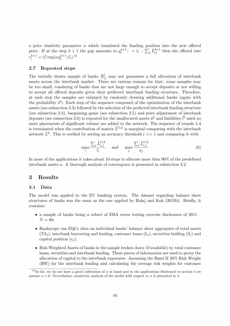
Figure 7 illustrates the impact of an adverse scenario on the interbank network structuresacross different network indicators, as compared to the end-sample starting point. Deviationsfrom the 45 degree line imply that the adverse shocks produce a different network configuration.Overall, it is difficult to gauge any systematic pattern in the responses of banks’ interlinkagesto the shocks. At the same time, it is notable that a considerable number of banks do deviatefrom the initial network characteristics, albeit the direction of the changes goes both ways.Some banks increase their degree of interconnectedness to the network, whereas other decreaseit. In other words, as should intuitively be expected, a change in the macro-financial situationwill endogenously lead to a change in network structures. We used statistical tests of differ-ences in mean (t test), variance (F test) and whole distribution (Kolmogorov-Smirnoff test) ofnetwork measures (in- and out-degree, Katz indicator, DebtRank and betweenness centrality)to verify changes in the network structures. At significance level of 5% only a hypothesisabout differences in variance of Katz ratio and betweenness cannot be rejected, i.e. a one-sided test indicates that in the adverse scenario some nodes become more interconnected withthe whole system comparing to the baseline case. At the level of 10% significance in-degreemeasure shows more connections in the system under baseline scenario (the average numberof linkages in the system is higher under the baseline). The outcomes of the statistical testsare intuitive. Under the adverse scenario, capital constraints and credit quality of some banksdeteriorate resulting in less potential for them to accept interbank deposits (binding capitalconstraint) or to be offered a placement (binding credit quality). The optimisation mechanismproposed in the framework nicely captures the relationship between macro-financial conditionsand network structures.

Apart from assessing whether adverse shocks impact the network formation process, ourmodel can also be employed to evaluate whether contagion losses under an adverse scenariocan be mitigated by adjusting certain regulatory (macro-prudential) instruments, such as largeexposure limits or for example risk weights on exposures to other financial institutions.

For example, Figure 8 illustrates the impact of having different LE limit thresholds in thecontext of an adverse shock. Specifically, the y-axis illustrates the difference between networksformed under a 15% LE limit and under the standard 25% LE limit in terms of the capitalloss following an adverse shock. A positive value implies that contagion losses rise when

27To insure robustness of the results a couple of adverse scenarios was applied.

24

Figure 7: Impact of the adverse scenario on the interbank network structures

−4 −3 −2 −1−4

−3.5

−3

−2.5

−2

−1.5

−1

OutDeg

−4 −3 −2 −1−4

−3.5

−3

−2.5

−2

−1.5

−1

InDeg

19 20 21 22 23 24 2519

20

21

22

23

24

25

DebtRank

−2 0 2 4−2

−1

0

1

2

3

4

Katz

Note: Each circle represents a measures for a bank in a network constructed under end-sample estimates

of the parameters (x-axis, log scale) and under an adverse scenario (y-axis, log scale). The size of a

circle is proportional to bank’s total assets.

Source: own calculations

25

Figure 8: Counterparty credit quality and the impact of LE limits on the losses incurred dueto contagion

0 500 1000 1500 2000 2500−3

−2.5

−2

−1.5

−1

−0.5

0

0.5

1

Note: x-axis: CDS spread (in bps). y-axis: difference of CAR after adverse stress testing shock between

LE=15% and LE=25% regime (in pp, positive number means that by lowering LE limit contagion losses

rise). No CVA adjustment (i.e. γ ≡ 0). The size of a circle is proportional to a bank’s total assets.

Source: own calculations

lowering the LE limit. On the x-axis, we plot the banks according to the size of their riskiness(measured in terms of their CDS spreads). It is observed that more stringent LE limits overalltend to lower contagion risk. Interestingly, this effect is especially pronounced for the groupof banks perceived (by the markets) to be the soundest. In other words, the forced reductionof counterparty concentration risk that would be implied by a lowering of the LE limits wouldseem to particularly benefit the safest part of the banking system whereas the more vulnerablesegments are found to be less affected by changes in the LE limits.

A similar analysis was carried out also for what concerns the CVA based add-on to the riskweights applied to the interbank exposures, see Figure 9. The Art. 458 of the CRDIV/CRR EUDirective28 defines a macro-prudential instrument of specific risk weights attached to exposuresto financial institutions. A rather broad formulation allows for a risk sensitive implementationof the instrument based on the CVA concept. In the context of our model, the parameter γplays a role of that special add-on. As was the case for the large exposure limits, the impact ofthe CVA on contagion risk is mainly affecting the sounder banks. In the case of the CVA basedadd-on, the direction of changes is however not unambiguous as we observe that depending onthe bank contagion risk can both increase and decrease when increasing the CVA charge.

28Directive 2013/36/EU of the European Parliament and of the Council of 26 June 2013 on access to the ac-tivity of credit institutions and the prudential supervision of credit institutions and investment firms, amendingDirective 2002/87/EC and repealing Directives 2006/48/EC and 2006/49/EC

26

Figure 9: Counterparty credit quality and the impact of CVA capital charge on the lossesincurred due to contagion

0 500 1000 1500 2000 2500−1.5

−1

−0.5

0

0.5

1

1.5

Note: x-axis: CDS spread (in bps). y-axis: difference of CAR after adverse stress testing shock between

CVA and no CVA regime (in pp, positive number means that introduction of CVA charge increases

contagion losses). LE= 25%. The size of a circle is proportional to a bank’s total assets.

Source: own calculations

5 Conclusions

In this paper, we have tried to deviate from the standard, mechanistic cascading mechanismemployed in traditional interbank contagion models. Instead, we have developed an agent-based model that is able to account for banks’ dynamic, endogenous responses both in theformation process of the interbank network and in response to contagious shocks.

Apart from analysing network formation processes and the implications for interbank con-tagion risks in a setting where banks are dynamically optimising their actions, our modelapproach can also be used to assess the impact of different regulatory and macro-prudentialpolicy instruments on the structure of interbank networks and their implied contagion risk.In this light, we presented a few policy experiments related to the effects of large exposurelimits on counterparty credit risks. These macro-prudential policy instruments were analysedboth in the context of network formation and in terms of their ability to mitigate interbankcontagion risks under adverse circumstances.

All in all, while the reported results obviously hinges on the specific characteristics of thebanks included in the network system and on the specific adverse scenarios considered, theoverriding conclusion from these policy experiments is that macro-prudential policies can makea significant difference through their impact on the network formation and ultimately on therisk of interbank contagion to adverse shocks. From this perspective, the modelling approachpresented in this paper can be employed for conducting impact assessments of selected macro-prudential policy instruments and in this way help inform the calibration of such tools.

27

Acknowledgements

The authors are indebted to I. Alves, S. Dubecq, J. Henry and other participants of an internalECB seminar who provided valuable comments and to VS Subrahmanian who discussed thepaper during INET conference in Ancona.

References

D. Acemoglu, A. Ozdaglar, and A. Tahbaz-Salehi. Systemic risk and stability in financialnetworks. Working Paper 18727, National Bureau of Economic Research, January 2013.URL http://www.nber.org/papers/w18727.

G. Afonso ad A. Kovner and A. Schoar. Stressed, not frozen: The federal funds market in thefinancial crisis. Journal of Finance, 66(4):1109–1139, 2011.

A. Adam. Handbook of Asset and Liability Management: From Models to Optimal ReturnStrategies. The Wiley Finance Series. John Wiley & Sons, 2008.

A. Babus. Endogenous intermediation in the over the counter markets. Working paper,Imperial College London, 2011.

A. Babus and P. Kondor. Trading and information diffusion in OTC markets. CEPR DiscussionPapers 9271, C.E.P.R. Discussion Papers, January 2013.

L. Balasubramanyan and D. VanHoose. Bank balance sheet dynamics under a regulatoryliquidity-coverage-ratio constraint. Journal of Macroeconomics, 37(0):53–67, 2013. ISSN0164-0704.

E. Baltensperger. Alternative approaches to the theory of the banking firm. Journal ofMonetary Economics, 6(1):1–37, January 1980.

BCBS. Basel III: A global regulatory framework for more resilient banks and banking systems.Technical report, Basel Committee on Banking Supervision, June 2011.

M. Bluhm, E. Faia, and P. Krahnen. Endogenous banks’ networks, cascades and systemicrisk. mimeo, Uni. Frankfurt, March 2013. URL http://www.wiwi.uni-frankfurt.de/

profs/faia/.

S.P. Borgatti and M.G. Everett. Models of core/periphery structure. Quantitative Finance,21:375–395, 1999.

M. Boss, H. Elsinger, S. Thurner, and M. Summer. Network topology of the interbank market.Quantitative Finance, 4:1–8, 2004.

J. H. Boyd and G. De Nicolo. The theory of bank risk taking and competition revisited. TheJournal of Finance, 60(3):1329–1343, 2005.

F. Brauning and F. Fecht. Relationship lending in the interbank market and the price ofliquidity. Discussion Papers 22/2012, Deutsche Bundesbank, Research Centre, 2012.

F. Castiglionesi and N. Lavarro. Fragile financial networks. Mimeo, Tilburg University, 2011.

28

F. Castiglionesi and W. Wagner. On the efficiency of bilateral interbank insurance. Journalof Financial Intermediation, forthcoming, 2013.

J. Chen and K. Song. Two-sided matching in the loan market. International Journal ofIndustrial Organization, 31:145–152, 2013.

F. Chung and L. Lu. Connected Components in Random Graphs with Given Expected DegreeSequences. Annals of Combinatorics, 6(2):125–145, November 2002. URL http://dx.

doi.org/10.1007/pl00012580.

E. Cohen-Cole, E. Patacchini, and Y. Zenou. Systemic risk and network formation in theinterbank market. CEPR Discussion Papers 8332, C.E.P.R. Discussion Papers, April2011.

D. Cuoco and H. Liu. An analysis of VaR-based capital requirements. Journal of FinancialIntermediation, 15(3):362–394, July 2006.

J. Danielsson, B. N. Jorgensen, and C. G. de Vries. Incentives for effective risk management.Journal of Banking & Finance, 26(7):1407–1425, July 2002.

H. Degryse and G. Nguyen. Interbank exposures: An empirical examination of systemic riskin the Belgian banking system. International Journal of Central Banking, 3(2):123–171,2007.

Deloitte and Solum Financial Partners. Counterpary risk and CVA survey. Survey February,Deloitte and Solum Financial Partners, 2013.

L. Eisenberg and T.H. Noe. Systemic risk in financial systems. Management Science, 47(2):236–249, February 2001.

J. Eisenschmidt and J. Tapking. Liquidity risk premia in unsecured interbank money markets.Working Paper 1025, European Central Bank, 2009.

E. Elyasiani, K. J. Kopecky, and D. van Hoose. Costs of adjustment, portfolio separation, andthe dynamic behavior of bank loans and deposits. Journal of Money, Credit and Banking,27(4):955–974, 1995. ISSN 00222879.

C. Ewerhart, N. Cassola, S. Ejerskov, and N. Valla. Liquidity, information and the overnightrate. Working Paper 378, ECB, 2004.

J. Fox. Estimating matching games with transfers. Working paper, Univertity of Michigan,2010.

C. Furfine. Interbank exposures: Quantifying the risk of contagion. Journal of Money, Creditand Banking, 35(1):111–638, 2003.

D. Gai and S. Kariv. Bayesian learning in social networks. Games and Economic Behaviour,45, 2003.

C.-P. Georg. The effect of the interbank network structure on contagion and common shocks.Discussion Paper Series 2: Banking and Financial Studies 2011,12, Deutsche Bundesbank,Research Centre, 12 2011.

29

M. Gofman. Effciency and stability of a financial architecture with too interconnected to failinstitutions. mimeo, University of Wisconsin-Madison, September 2013.

M. Grasselli. An agent-based computational model for bank formation and interbank networks.In J.-P. Fouque and J. Langsam, editors, Handbook on Systemic Risk, 2013.

M. Gross and C. Kok. Measuring contagion potential among sovereigns and banks using amixed-cross-section GVAR. mimeo (forthcoming in the ecb working paper series), Euro-pean Central Bank, March 2013.

G. Ha laj. Optimal asset structure of a bank – bank reactions to stressful market conditions.ECB Working Paper Series) 1533, European Central Bank, April 2013.

G. Ha laj and Ch. Kok. Assessing interbank contagion using simulated networks. ECB WorkingPaper Series 1506, European Central Bank, January 2013a.

G. Ha laj and Ch. Kok. Assessing interbank contagion using simulated networks. ComputationalManagement Science, 10(2-3):157–186, 2013b.

J.D. Hamilton. Measuring the liquidity effect. American Economic Review, 87(1):80–97, 1998.

F. Heider, M. Hoerova, and C. Holthausen. Liquidity hoarding and interbank market spreads.Working Paper 1107, ECB, 2009.

R. A. Howard and J. E. Matheson. Risk-sensitive markov decision processes. ManagementScience, 18(7):356–369, 1972. ISSN 00251909.

G. Iori, S. Jafaray, and F. Padilla. Systemic risk on the interbank market. Journal of EconomicBehavior and Organization, 61:525–542, 2006.

M.O. Jackson and A. Wolinsky. A strategic model of social and economic networks. Journal ofEconomic Theory, 71(1):44–74, October 1996. URL http://ideas.repec.org/a/eee/

jetheo/v71y1996i1p44-74.html.

S. Markose. Systemic risk from global financial derivatives: A network analysis of contagionand its mitigation with super-spreader tax. Working Paper 12/282, IMF, 2012.

M.E.J. Newman. Random graphs with clustering. Physical Review Letters, 103(5), 2009.

E. Nier, J. Yang, T. Yorulmazer, and A. Alentorn. Network models and financial stability.Journal of Economic Dynamics and Control, 31(6):2033–2060, 2007.

L. Pelizzon and S. Schaefer. Pillar 1 vs. Pillar 2 under risk management. NBER WorkingPapers 11666, National Bureau of Economic Research, Inc, October 2005.

J.-C. Rochet and J. Tirole. Interbank lending and systemic risk. Journal of Money, Creditand Banking, 28(4):733–762, 1996.

K. Soramaki, M.L. Bech, J. Arnold, R.J. Glass, and W.E. Beyeler. The topology of interbankpayment flows. Physica A, 379:317–333, 2007.

C. Upper and A. Worms. Estimating bilateral exposures in the German interbank market: Isthere a danger of contagion? European Economic Review, 48(4):827–849, 2004.

30

I. van Lelyveld and F. Liedorp. Interbank contagion in the Dutch banking sector: A sensitivityanalysis. International Journal of Central Banking, 2(2), May 2006.

A Credit Valuation Adjustment

The (OTC) interbank exposures carry risk related to the counterparts default. Banks willbe obliged under Basel III agreement to quantify that risk by calculating the so-called CreditValuation Adjustment (CVA) based on the market parameters reflecting market participants’perception of counterpart credit risk.29 The advanced method of CVA calculation involves theobserved credit default spreads of the counterparts to infer the market-based probability ofdefault and consequently, given the assumed exposures and their maturities, the expected losson the portfolio of the interbank assets. The CVA will become the additional capital chargefor unhedged counterparty risk related to the OTC exposures (balance and off-balance). TheCVA term is calculated in the following way :

CVA = λ∑n≤N

(exp(−sntn/λ)− exp(−sn−1tn−1/λ)

)(EEnd

n + EEn−1dn−1)/2,

where λ is the market based assessment of the loss given default on the exposure against agiven counterparty, tn is the n-th point of time, cdsn is the projected CDS spread at time n,EEn is the projected, netted exposure against the counterparty and dn is a discount factor.Consequently, CVA accounts for the mark-to-market losses on the counterparty risk. If notavailable on the bank specific level, Basel iii allows for it to be replaced by an aggregate onebased on rating, industry and region. Notably, the formula can be used by IRB banks and thenthe main difficulty of its implementation is finding appropriate profile for EE (in particularmaturity tN ). The standardised approach banks are required to apply a simplified formula forwhich the profile of EE does not matter but still the maturity has to be imposed (at least thecontractual of the analysed EAD).

We assume that the netted exposures of a given bank are constant within a given horizontN . It means that EEn is constant, EEn = EE∗ and the vector of proportionality parametersγ used in the definition of the capital constraints have entries defined as:

γi : =CV Ai

EE∗= λ

∑n≤N

(exp(−si,ntn/λ)− exp(−si,n−1tn−1/λ)

)(dn + dn−1)/2

B Modified Jaccard index – similarity of networks

In order to measure similarities between networks structures one can apply the so-called Jac-card index. It counts the number of linkages that appear in the two compared networks andrelates it to the total number of linkages in both graphs. It therefore neglects the weight ofthe links, i.e. the importance of the overlapping linkages relative to the once uniquely presentin one of the networks. We propose a slight modification to the index accounting for that

29The most recent proposal can be found under the following address: http://www.bis.org/publ/bcbs227.htm

31

deficiency. For the 2 given networks N1 and N2 described by weighted adjacency matrices M1

and M2, span on the same set of N nodes, let us define 3 sets:

M12: = (i, j) ∈ N× N|(i, j) ∈ N1 ∧ (i, j) ∈ N2M10: = (i, j) ∈ N× N|(i, j) ∈ N1 ∧ (i, j) /∈ N2M02: = (i, j) ∈ N× N|(i, j) /∈ N1 ∧ (i, j) ∈ N2

They describe the number of links that overlap between the graphs (M12) and those thatare present in on graph but not in the other (M10 and M02). The modified Jaccard index(Jm(N1,N2)) is defined as:

Jm(N1,N2) =#M12

∑(i,j)∈M12(M1

i,j +M2i,j)∑

Z∈M12,M10,M02

(#Z

∑(i,j)∈Z(M1

i,j +M2i,j)) (7)

The number of linkages within a given group (M12, M10 or M02) are weighted by the sum ofexposures related to that links reflecting the importance of a given group of links.

C Covariance of the funding risk X

Default probabilities pj are modelled as random variables with variance estimated based on atime series of CDS spreads. Let (Ω,F ,P) be a probability space containing correlated randomvariables pj taking values from [0,1] and independent (pairwise and with all pjs) randomvariables uj , uniformly distributed on [0,1]. Let us define the σ-field generated by pjs, i.e.

Fp = σ(p−1j (C)|j ∈ N ∧ C ∈ B([0, 1])

),

where B([0, 1]) is a σ-field of Borel set on [0,1]. We use throughout the derivation the followingfact:

For two given random variables Y1 and Y2, a σ-field G, such that Y1 is G-measurableand Y2 is independent of G and an integrable function f ,

E[f(Y1, Y2)|G] = E[f(y, Y2)]|y=Y1

The proof of the fact is standard: first for the elementary functions, then for their linearcombinations and finally in the closure of the resulting subspace in L1(F).

Additionally,Xj : = E [Xj |Fp] = 1− pj

since Fp is independent of uj .Case i 6= j

cov(Xi, Xj) = E [(Xi −EXi)(Xj −EXj)] = E[E[XiXj −EXiEXj |Fp

]]= E

[E[Iui>piIuj>pj

] ∣∣∣(pi,pj)=(pi,pj)

]− (1−Epi)(1−Epj)

(8)

32

the last equality once again following independence of ui, uj and Fp. Then, following inde-pendence of ui and uj

= E(1− pi)(1− pj)− (1−Epi)(1−Epj) = Epipj −EpiEpj = cov(pi, pj) (9)

Case i = j

cov(Xi, Xi) = E[(Iui>pi

)2]− (1−Epi)2

Since Iui>pi takes only values 0 and 1, the square can simply be omitted in the first termunder the expectation operator yielding

= (1−Epi)− (1−Epi)2 = Epi − (Epi)

2 (10)

D Setup and solution to the bargaining game

The aim of the bargaining game defined for all pairs of banks is to find an agreements betweenthe offers of interbank placements and interbank funding needs. The key parameters to definethe game are the sensitivities of a bank’s optimised functional to a move from the optimum tothe second player’s optimum.30 The asset side bank’s satisfaction is measured by risk-adjustedreturn at the optimal allocation. The funding side bank’s utility is gauged by the variance ofthe funding portfolio. Let us focus on a pair (i, j). Bank j is a lender, i is a borrower. For

the bank j we define a function of its satisfaction Ua,kij given a placement x to bank i ceteris

paribus, i.e other volumes retained at the optimum level. Formally,

Ua,kij (x) = J(LI,k

1j , . . . , LI,ki−1j , x, L

I,ki+1j , . . . , L

I,kNj)

Analogously, the utility U l,kij of the bank borrower i accepting placement x from bank j is

measured at the optimal funding volumes from all other banks than j:

U l,kij (x) = −F (LF,k

i1 , . . . , LF,kij−1, x, L

F,kij+1, . . . , L

F,kiN )

Obviously, Ua,k∗ij = Ua,k

ij (LI,kij ) and U l,k∗

ij = U l,kij (LF,k

ij ) are the measures of satisfaction at theoptimum.

If LI,kij 6= LF,k

ij then we define sensitivity measures of satisfaction of player j moving from the

individually optimal allocation LI,kij to LF,k

ij and player i changing the funding volume obtained

from player j from LF,kij to LI,k

ij . We measure the sensitivity by means of the following ratios:

sa,kij = max

(Ua,kij (LI,k

ij )− Ua,kij (LF,k

ij )

|LF,kij − L

I,kij |

, 0

)(11)

sl,kij = max

(U l,kij (LF,k

ij )− U l,kij (LI,k

ij )

|LI,kij − L

F,kij |

, 0

)(12)

30We prefer this definition of sensitivity to an alternative one based on a unit change or derivative to mitigateproblems of missing second order terms. Notably, the optimised functionals in round 1 and 2 are quadratic.

33

In this way, we implicitly assume that banks’ dissatisfaction from abandoning the optimisation-based investment and funding portfolios is growing linearly along the allocation between LI,k

ij

and LF,kij . The max operation accounts for the fact that actions LI,k

ij and LF,kij are not globally

optimal but rather on a constraint set of strategies.In the interbank bargaining game at round k banks maximise the utility functional Gk

ij

defined:Case 1: LI,k

ij > LF,kij ⇒

Gkij(x) =

[U l,k∗ij − sl,kij · (x− L

F,kij )

] [Ua,k∗ij − sa,kij · (L

I,kij − x)

](13)

maximised on [LF,kij , LI,k

ij ]

Case 2: LI,kij < LF,k

ij ⇒

Gkij(x) =

[Ua,k∗ij − sa,kij · (x− L

I,kij )] [U l,k∗ij − sl,kij · (L

F,kij − x)

](14)

maximised on [LI,kij , L

F,kij ]

After basic calculations, the solution can simply be written as:Case 1: the bargaining game equilibrium allocation LG,k satisfies:

LG,kij = max(min(xk∗ij , L

I,kij ), LF,k

ij )

where

xk∗ij =1

2

[LF,kij + LI,k

ij +U l,k∗ij

sl,kij−Ua,k∗ij

sa,kij

]Case 2: the bargaining game equilibrium allocation LG,k satisfies:

LG,kij = max(min(xk∗ij , L

F,kij ), LI,k

ij )

where

xk∗ij =1

2

[LF,kij + LI,k

ij +Ua,k∗ij

sa,kij

−U l,k∗ij

sl,kij

]On aggregate, the outcome of the bargaining game may violate the ak and lk constraint,

since∑

i LG,kij′ > aj′ for some j′ and

∑j L

G,ki′j > li′ for some i′. Therefore, rows and columns of

LG,k are transformed proportionately:

LG,kij → LG,k

ij : = LG,kij ·min(1,

lki∑j L

G,kij

),

LG,kij → LG,k

ij : = LG,kij ·min(1,

akj∑i L

G,kij

)

The ultimate matrix of exposures LG,k realised in the step k is defined as the element-wiseminimum of LG,k and LG,k:

LG,kij = min(LG,k

ij , LG,kij )

34

Figure 10: Incompletness of the interbank network structure with the estimated correlation ofrisks

AT

AT

AT

BE BE

CY CY

DEDEDEDE

DEDE

DEDE

DE DE DEDE

DE

DK

DK

DK

DK

ES

ESES

ESESESES

ES

ES

ES

ESES

ES ES ESES

ES

ES

ES

FR

FR

FR

FR

GB

GB

GB

GB

GR

GR

GR

GR

HU

IE

IE

IE

ITIT

ITIT

IT

LU

NL

NL

NL

NL

NO

PT

PT

PT

PT

SE

SE

SE

SE

SI SI

Note: The darker the line, the higher the probability that the link exists. The circles around the nodes

indicate bank sizes (proportional to log of total assets).

Source: own calculations

D.1 Sensitivity analysis

To make sure that policy conclusions we draw are robust, we assess performance of the modelverifying the interbank structures it produces and their sensitivity to key driving parameters,such as correlation (Q), loss given default (λ), investment risk aversion (κ), funding riskaversion (κF ), interbank interest rate elasticity (α) and capital allocated to the interbankportfolios (eI).

One particular interbank structure estimated in the developed endogenous network modelis presented in Figure 10. It is incomplete with the largest banks being the most interconnectednodes, which is in line with findings elsewhere in the literature.31

The correlation structure should in theory influence the concentration and completenessof the interbank network. Notably, from the perspective of the optimal asset structures, highcorrelation translates into low diversification potential implying that the assets are optimallyallocated in just a few banks. However, it is not a priori clear how the network structures mayrespond to the increasing correlation of the interests paid by the interbank deposits. Figures11 and 12 synthetically show sensitivities of some basic (and commonly used) topologicalmeasures of networks to the decreasing correlation. The systemic importance of some nodesgradually increases as the correlation falls from the estimated one to the state where there isno dependence between interbank interest rates (and default risk that influences the cost offunding). This is slightly more persistent for the larger banks whereas some of the small banks

31For a few representative country-specific studies using real-time overnight transactions data or large expo-sure data as well as entropy approaches, see e.g. Furfine (2003), Upper and Worms (2004), Boss et al. (2004),van Lelyveld and Liedorp (2006), Soramaki et al. (2007) and Degryse and Nguyen (2007).

35

Figure 11: In-degree of banks in the simulated system vs the strength of correlation

0.2 0.3 0.4 0.5 0.6 0.7 0.8 0.9 10

0.05

0.1

0.15

0.2

0.25

0.3

0.35

0.4

Note: x-axis: factor reducing the correlation of risk between banks, e.g. 0.4 means that the applied

correlation matrix Q0.4 is such that for all i 6= j Q0.4(i, j) = (1− 0.4)Q(i, j). The darker the line, the

larger the bank. Investment risk aversion κ = 1. Funding sources diversification parameter is set to

0.5. No CVA adjustment (i.e. γ ≡ 0).

Source: own calculations

react strongly as the correlation becomes close to 0 by spreading their interbank assets morewidely across the system.

Given that the two measures of interconnectedness indicate the increase of linkages ascorrelation vanishes, it is interesting to study the importance of the sizes of linkages and thegeneral network structure differences. In order to address the issues we plotted the distri-bution of the interbank exposures for different strengths of the correlation (see figure 13).The estimated dependence of the return and risk parameters of the interbank deposits, whichis relatively high due to the correlation of the reference interest rates, leads to network withmany banks connected by some very large exposures comparing to the median. As the correla-tion decreases, the network become more and more homogenous in terms of interbank depositvolumes. Notably, in general the size of exposures decreases.

The interbank networks may thus differ a lot for different degrees of correlation. However,it can be observed that the largest linkages, contributing to the core structure of the interbankgraph, are generally stable and that the differences are related mainly to the smaller depositamounts. This is illustrated in the lower pane of figure 14. We compared the original Jaccardindex based on the adjacency matrix with a modified one accounting for the sizes of theexposures. It is observed that the curve produced by the modified index lies above the oneobtained from the original one indicating that the linkages among the largest banks are morestable (i.e. less sensitive to correlation). This notwithstanding, in general correlation appearsto have a sizable impact on the structure of the endogenous network formation.

There are several key parameters of the model that were set in an arbitrary way. We

36

Figure 12: Out-degree of banks in the simulated system versus the strength of correlation ofinterbank returns

0.2 0.3 0.4 0.5 0.6 0.7 0.8 0.9 10

0.05

0.1

0.15

0.2

0.25

0.3

Note: The darker the line, the larger the bank. Investment risk aversion κ = 1. Funding sources

diversification parameter is set to 0.5. No CVA adjustment (i.e. γ ≡ 0)

Source: own calculations

Figure 13: Distribution of linkages in the network vs correlation of the combined interest rateand counteparty risk

estim. correlation3

3.5

4

4.5

5

5.5

6

no correlation3

3.5

4

4.5

5

5.5

6

Note: y-axis: log size of exposures. Upper and bottom lines of the box reflect 75th and 25th percentile,

the line inside the box – the median.

Source: own calculations

37

Figure 14: Network similarity measures versus the strength of the correlation.

0 0.1 0.2 0.3 0.4 0.5 0.6 0.7 0.8 0.9 1

0.65

0.7

0.75

0.8

0.85

0.9

0.95

1

Note: x-axis: factor reducing the correlation of risk between banks, e.g. 0.4 means that the applied

correlation matrix Q0.4 is such that for all i 6= j Q0.4(i, j) = (1 − 0.4)Q(i, j). dashed line – Jaccard

index, solid line – modified Jaccard index (taking into account the size of the exposures (see Appendix

B)).

Source: own calculations

Table 1: Sensitivity of networks structures to parameters

Network measure – avg. weighted relative change vs base-line (%)

Parameter (baseline) Tested value Out-deg In-deg Bness Katz DebtRank

LGD (0.4)0.3 -1.6 0.2 1.3 1.5 2.3

(0.1 ) (0.4 ) (0.0 ) (0.3 ) (0.1 )0.5 1.8 -0.8 -0.5 -1.4 -0.1

(0.2 ) (0.3 ) (0.1 ) (0.1 ) (0.0 )Inv. risk aversion (0.5)

1.5 -3.0 -1.0 0.2 0.5 0.9(0.1 ) (0.2 ) (0.5 ) (0.1 ) (0.3 )

2.5 -3.7 -1.0 -4.2 0.7 1.2(0.1 ) (0.1 ) (0.7 ) (0.2 ) (0.2 )

Fund. risk aversion (0.5)1.5 1.2 0.1 3.4 5.2 3.8

(0.5 ) (0.0 ) (0.5 ) (0.8 ) (0.6 )2.5 2.3 0.1 5.6 5.6 3.7

(0.7 ) (0.0 ) (0.6 ) (0.7 ) (0.1 )Price elast. (0.0)

0.5 4.1 5.2 10.3 -0.6 -1.8(1.7 ) (0.6 ) (2.4 ) (0.3 ) (0.1 )

1.0 4.4 -2.3 12.8 3.2 -1.7(0.5 ) (0.4 ) (1.9 ) (0.3 ) (2.1 )

Alloc. capital (eI)0.9eI 2.6 0.6 10.0 -4.2 -3.7

(0.2 ) (0.3 ) (0.6 ) (0.7 ) (0.8 )1.1eI 5.9 3.4 3.7 -1.6 -2.7

(0.3 ) (0.3 ) (0.6 ) (0.6 ) (0.5 )

Note: relative change with respect to baseline value of the tested parameter; standard deviations inbracketsSource: own calculations

38

Figure 15: Distribution of Bargaining Game adjustment factors

0 0.1 0.2 0.3 0.4 0.5 0.6 0.7 0.8 0.9 1

0

0.2

0.4

0.6

0.8

1

Note: adjustment factor: min(1,lki∑

j LG,kij

) for any index j; distribution based on a simulation of 50

networks of 80 banks with 20 steps of optimisation of assets and liabilities followed by bargaining game

⇒ 80000 calculated ratios.

Source: own calculations

address the issue of how sensitive the results are to the chosen specification and present theresults in Table 1. The structure of the endogenously derived interbank network is mostsensitive to deposit interest rate elasticity and the level of allocated capital to the interbankportfolios. It is most evident for the number of linkages between banks (in- and out-degreemeasures) and betweenness centrality. In general, however, the structures vary in a limitedway and the variability that we do observe tends to have intuitive explanations. For instance,increasing investment risk aversion leads on average to the decrease in the number of linkagesas measured by in- and out-degree. Consequently, some nodes in the network become moresystemic, which can be measured by Katz and DebtRank indicators detecting nodes-hubs thatdirectly and indirectly connect banks in the network.

The proportionate transformation LG → LG is designed to ensure that the budget con-straint of total interbank assets a and liabilities l is satisfied after the bargaining game butmay distort the outcomes of the game. We verified in how many instances the proportionaladjustment is activated. As shown in figure 15 in more than 80% of cases no adjustment isrequired and the remaining part of the distribution is spread uniformly in [0, 1] interval ofadjustments.

39