University of Illinois at Urbana-Champaign, Urbana, IL 61801, USA
This paper focuses on full six degree-of-freedom (6-DOF) aerodynamic modelingof small UAVs at high angles of attack and high sideslip in maneuvers performed us-ing large control surfaces at large deflections for aircraft with high thrust-to-weightratios. Configurations such as this include many of the currently available propeller-driven RC-model airplanes that have control surfaces as large as 50% chord, deflec-tions as high as 50 deg, and thrust-to-weight ratios near 2:1. Airplanes with thesecapabilities are extremely maneuverable and aerobatic, and modeling their aerody-namic behavior requires new thinking because using traditional stability derivativemethods is not practical with highly nonlinear aerodynamic behavior and coupling inthe presence of high propwash effects. The method described in this paper outlines acomponent-based approach capable of modeling these extremely maneuverable smallUAVs in a full 6-DOF realtime environment over the full envelope that is definedin this paper to be the full ±180 deg range in angle of attack and sideslip. Thismethod is the foundation of the aerodynamics model used in the RC flight simula-tor FS One. Piloted flight simulation results for four small RC/UAV configurationshaving wingspans in the range 826 mm (32.5 in) to 2540 mm (100 in) are presentedto highlight results of the high-angle aerodynamics modeling approach. Maneuverssimulated include tailslides, knife edge flight, high-angle upright and inverted flight(“harriers”), rolling maneuvers at high angle (“rolling harriers”) and an invertedspin of a biplane (“blender”). For each case, the flight trajectory is presented to-gether with time histories of aircraft state data during the maneuvers, which arediscussed.
Nomenclature
A = propeller disc areaa = airfoil lift curve slope (2π)c = mean aerodynamic chord; camberCd = drag coefficientCl = lift coefficientCQ = propeller torque coefficient (Q/ρn2D5)CT = propeller thrust coefficient (T/ρn2D4)Cm,c/4 = moment coefficient about quarter chordD = drag; propeller diameterJ = propeller advance ratio based on VN
L = liftM = pitching moment about y-axis (positive nose up)n = propeller rotational speed (revs/sec)
∗Associate Professor, Department of Aerospace Engineering, 104 S. Wright St. Senior Member AIAA.http://www.ae.illinois.edu/m-selig
1 of 35
American Institute of Aeronautics and Astronautics
NP = propeller yawing moment due to angle of attackp, q, r = roll, pitch and yaw ratePN = propeller normal force due to angle of attackQ = propeller axial torqueq = dynamic pressure (ρV 2/2)R = propeller radiusS = reference areaT = propeller axial thrustu, v, w = components of the local relative flow velocity along x, y, z, respectivelyV = flow velocityx, y, z = body-axis coordinates, +x out nose, +y out right wing, +z downyc = airfoil camberTED = trailing edge downTEL = trailing edge leftTEU = trailing edge up
Subscripts
N = normal componentR = relative component
Symbols
α = angle of attack (arctan(w/u))β = sideslip angle (arcsin(v/V ))β′ = angle of attack for vertical surface (arctan(v/u))δa = aileron deflection [(δa,r − δa,l)/2], right +TEU, left +TEUδe = elevator deflection, +TEDδr = rudder deflection, +TELǫ = wing induced angle of attackηs = dynamic pressure ratio for flow shadow (shielding) effectφ, θ, ψ = bank angle, pitch angle, heading angleρ = air densityσ = propeller solidity (blade area/disc area)
Superscripts
( ) = normalized quantity; average quantity
I. Introduction
There is growing interest in modeling and understanding full-envelope aircraft flight dynamics, that is,modeling the aircraft over the full ±180 deg range in angle of attack and sideslip. Flight outside the normalenvelope like this can be encountered in airplane stall/spin situations or more generally upset scenarios thatcan be caused by a host of factors – pilot, aircraft, weather, etc. Moreover, aerobatic airplanes routinelyenter and exit controlled flight “outside-the-envelope” with precision and grace. Interest in full-envelopeaircraft flight dynamics has also been fueled in recent years by the rapid growth in UAVs (both civilian andmilitary) together with synergistic parallel advances in high-performance RC model aircraft.
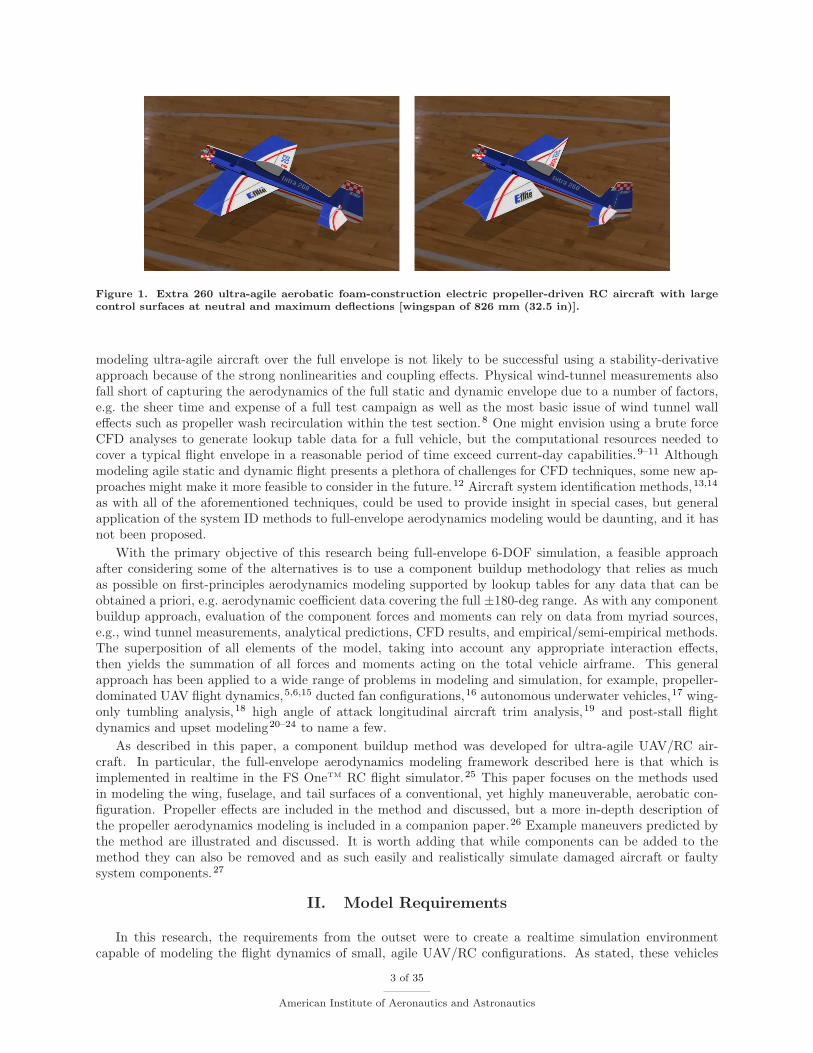
Within the broad spectrum of UAV/RC configurations has emerged a general category that is capableof extremely agile maneuvers such as V/STOL-like flight, hovering, perching, stop-and-stare, defensive andevasive postures and rapid roll, pitch, yaw rates and accelerations.1–7 The high agility derives from havingcontrol surfaces as large as 50% chord with deflections as high as ±50 deg and propeller thrust-to-weightratios of near 2:1. A tractor-propeller-driven fixed-wing RC variant that falls in this category is shown inFigure 1 with the large control surfaces at neutral and then deflected to illustrate their full extent.
These ultra-agile configurations clearly present new challenges to flight dynamics simulation and model-ing because of the combined considerations of high-angle full-envelope flight, large highly-deflected controlsurfaces, strong propeller wash effects, high thrust and concomitant unsteady flow. In the general case,
2 of 35
American Institute of Aeronautics and Astronautics
Figure 1. Extra 260 ultra-agile aerobatic foam-construction electric propeller-driven RC aircraft with largecontrol surfaces at neutral and maximum deflections [wingspan of 826 mm (32.5 in)].
modeling ultra-agile aircraft over the full envelope is not likely to be successful using a stability-derivativeapproach because of the strong nonlinearities and coupling effects. Physical wind-tunnel measurements alsofall short of capturing the aerodynamics of the full static and dynamic envelope due to a number of factors,e.g. the sheer time and expense of a full test campaign as well as the most basic issue of wind tunnel walleffects such as propeller wash recirculation within the test section.8 One might envision using a brute forceCFD analyses to generate lookup table data for a full vehicle, but the computational resources needed tocover a typical flight envelope in a reasonable period of time exceed current-day capabilities.9–11 Althoughmodeling agile static and dynamic flight presents a plethora of challenges for CFD techniques, some new ap-proaches might make it more feasible to consider in the future.12 Aircraft system identification methods,13,14
as with all of the aforementioned techniques, could be used to provide insight in special cases, but generalapplication of the system ID methods to full-envelope aerodynamics modeling would be daunting, and it hasnot been proposed.
With the primary objective of this research being full-envelope 6-DOF simulation, a feasible approachafter considering some of the alternatives is to use a component buildup methodology that relies as muchas possible on first-principles aerodynamics modeling supported by lookup tables for any data that can beobtained a priori, e.g. aerodynamic coefficient data covering the full ±180-deg range. As with any componentbuildup approach, evaluation of the component forces and moments can rely on data from myriad sources,e.g., wind tunnel measurements, analytical predictions, CFD results, and empirical/semi-empirical methods.The superposition of all elements of the model, taking into account any appropriate interaction effects,then yields the summation of all forces and moments acting on the total vehicle airframe. This generalapproach has been applied to a wide range of problems in modeling and simulation, for example, propeller-dominated UAV flight dynamics,5,6,15 ducted fan configurations,16 autonomous underwater vehicles,17 wing-only tumbling analysis,18 high angle of attack longitudinal aircraft trim analysis,19 and post-stall flightdynamics and upset modeling20–24 to name a few.
As described in this paper, a component buildup method was developed for ultra-agile UAV/RC air-craft. In particular, the full-envelope aerodynamics modeling framework described here is that which isimplemented in realtime in the FS OneTM RC flight simulator.25 This paper focuses on the methods usedin modeling the wing, fuselage, and tail surfaces of a conventional, yet highly maneuverable, aerobatic con-figuration. Propeller effects are included in the method and discussed, but a more in-depth description ofthe propeller aerodynamics modeling is included in a companion paper.26 Example maneuvers predicted bythe method are illustrated and discussed. It is worth adding that while components can be added to themethod they can also be removed and as such easily and realistically simulate damaged aircraft or faultysystem components.27
II. Model Requirements
In this research, the requirements from the outset were to create a realtime simulation environmentcapable of modeling the flight dynamics of small, agile UAV/RC configurations. As stated, these vehicles
3 of 35
American Institute of Aeronautics and Astronautics
have high thrust-to-weight ratios near 2:1 and use large control surfaces at high deflections immersed instrong propeller wash. Consequently, the trimmable flight envelope is large, and the range of dynamicmaneuvers is spectacular.
The trimmable flight envelope to be captured in simulation includes all of the nominal trimmed states,e.g., straight flight and turning flight. While normal cruise flight is the nominal condition, these highlymaneuverable UAV/RC aircraft can fly outside the envelope in trim at high angles of attack near 45 degwith large nose-up elevator input – the so-called “harrier” maneuver in RC parlance. This flight conditionrelies on lift from the wing and also the vertical component of thrust to sustain level trimmed flight. Takenfurther with more nose-up elevator and additional thrust the flight can be arrested to a 90-deg angle of attackstationary hovering attitude that uses only thrust to support the aircraft weight. This hover condition canalso be entered from steady knife-edge flight that is extended with large rudder input to an extreme 90-degyaw that again ends in a stationary hovering attitude. All of these conditions were required to be capturedin the simulation.
Apart from trimmed flight, other dynamic maneuvers to be captured by the simulation are much morecomplex. These include the classic stall from upright longitudinal flight and also wing tip stall that canprecipitate into a fully-developed spin. The spin can be characterized by a number of descriptors, e.g., itcan be an upright spin or inverted spin with either a nose-down attitude or flat spin with power added ornot, all resulting in extremely complex aerodynamic states to model. “Blender” is the particular name givento inverted power-on flat spins that are dramatic, and this same maneuver can be entered and momentarilysustained from a level high-speed flight condition. Snaps, tailslides, hammerheads and knife edge stall are alsodynamic maneuvers that are aerobatic in nature and lead to high-angle flight conditions. Modern RC modelswith high thrust capabilities can also perform what are called “rolling harriers,” which is a high angle of attackslow roll condition that requires modulating elevator and rudder input (out-of-phase) to keep a nose-highattitude while simultaneously rolling with near constant aileron input. These rolling harriers can be flownin straight flight, turning flight, loops or horizontal (or vertical) figure eights, etc. Other rapid maneuvers toextreme angle are “walls” (rapid pitch up from level flight to an arrested hovering position), “parachutes”(rapid pitch to level from a vertical downline), and “elevators” which is a deep-stall descent attitude. Apartfrom upset conditions that are accidentally encountered, these aerobatic dynamic maneuvers and others thatare well known (e.g., torque rolls, “waterfalls” and knife-edge loops) clearly depend on varying degrees ofpilot skill to perform. Simulating these maneuvers poses unique and formidable challenges in aerodynamicsmodeling.
Other simulation requirements factored into the original design and having impact on the aerodynamicsmodeling included the following. First, the environment was required to be capable of simulating manydifferent aircraft and thus not be tailored to capturing only the flight dynamics of certain special maneuversunique to one or a few aircraft. Second, simulating the effects of damage or missing parts (e.g., a failed aileronor a missing wing) was key initially because of the commercial market appeal, but including these featureshas longer reach and applies to failures of full-scale aircraft as well. Third, the simulation environment wasrequired to allow for automatic scaling of any native aircraft to any other size, e.g., nano-scale, micro-scale,50%-scale and full-scale. Fourth, because typical small aircraft are subject to relatively high atmosphericturbulence, a robust wind and turbulence model was required in the simulation.
Finally, the simulation framework (including graphics, physics, pilot inputs, recording features, andmore) was required to run in realtime on a standard gaming-level desktop PC. Clearly, this computationalenvironment set additional requirements on the aerodynamics modeling methodology to make it robust andalso capable of simulating nominal, agile and aerobatic flight over a range of situations. The remainder ofthis paper henceforth will focus on the aerodynamics modeling and simulation that achieves all of the broadrequirements that have been outlined in this section.
III. Technical Development Process
The development began with a relatively simple and general approach – that of using stability derivatives.However, during the core development period (3 yrs), each element of the stability derivative approach wasreplaced by methods that could capture the full envelope with enough generality to simulate flight in anyattitude.
Out of this fundamental bottom-up approach arose the capability to simulate highly nonlinear complex
4 of 35
American Institute of Aeronautics and Astronautics
maneuvers that are observed in actual flight across a spectrum of aircraft. In fact, the framework wasapplied equally across an array of more than 30 aircraft covering myriad configurations that ranged fromsimple rudder-elevator glider trainers to ones having propulsion (jet and propeller) with large flaps, ailerons,elevator, and airbrakes.25 The technical development also directly benefited from and depended on theauthor’s 40-yr experience with flying and observing model aircraft as well as physical measurements, flightvideo and feedback from professional RC pilots and aircraft designers.
IV. Component Aerodynamics Models
In the model, the aircraft is divided into basic components such as the wing, horizontal tail, verticaltail, propeller, etc., and for each a separate model is developed to determine the contribution that eachcomponent makes to the total forces and moments on the aircraft at each point in time. For each component,the local relative flow is determined taking into account aircraft speed and rotations (assuming rigid bodykinematics) together with wind, turbulence and any aerodynamic interference effects such as propeller wash,wing induced flow, shielding effects (e.g., tail blanketing in spin), ground effect and more. For most of themodels, the component state (relative flow, surface deflections, and other data as it might apply) is then usedto determine any related aerodynamic coefficient data. The final component dynamic pressure, aerodynamiccoefficient data and respective reference area are then used to determine the forces and moments. This basicapproach applies to the simplest component models, while in most cases additional steps are taken or anentirely different approach is used involving analytical and/or empirical/semi-empirical methods built uponsome physical basis.
A. Wing Aerodynamics
The wing aerodynamics produce the most dominant forces and moments, and thus careful modeling is keyto simulating full vehicle performance. Challenges in predicting this performance include mainly high angle(±180 deg) performance and large control surfaces at high deflections. Other important elements includewing-in-propeller slipstream effects, induced flow produced by the wing, shielding of one wing on another(biplane wings), apparent mass and flow curvature effects. In most cases the reduced frequency in pitch issmall enough that dynamic stall effects are small, and thus this effect is not currently included in the model.
In order to run in realtime, there must be a balance between using on-the-fly fundamental physics methodsand pre-computed data that can be accessed quickly through lookup tables. For the wing, this precomputeddata includes the full aerodynamic coefficients (Cl, Cd, Cm,c/4) and induced angle of attack as a function ofany control surface deflections. These data are local values at stations along the wing, that is, the wing isdiscretized and in the simulation a strip theory approach is applied as will be described.
As a method, strip theory is used for aircraft aeroelastic simulations28 and routinely for blade elementtheory in the rotorcraft field.29 Strip theory approaches have also been applied to wings in a trailing vortexflow and aircraft spin prediction (see Refs. 30–33 and others cited therein). It seems that only recentlyhas the general strip theory approach been applied in realtime simulation for fixed-wing force and momentcalculations.6,23,24†
Various approaches to implementing a strip theory approach have been applied for fixed and rotary wingaircraft. In this work, the approach is to use a nonlinear lifting line code to determine the local inducedangle of attack at each section along the wing over a range of angles of attack and control surface deflections.Thus, lookup tables are created for the local 2D induced angle ǫ as a function of the local 2D angle ofattack α and local control surface deflection. In the method, the local 3D flow for an element of the wing iscomposed of the sum of all velocity components due to aircraft motion, propeller wash, and wind along withcorrections for any shielding that might be modeled on the element. From this direct flow calculation, thelocal 2D angle of attack is obtained and used to find induced angle through lookup tables. A ground effectcorrection is also applied when in ground proximity. Taking all these contributions into account, the angleof attack of the relative flow becomes
α = αdirect flow + ǫ+ ∆αground effect (1)
†In this work in the development of FS One, the strip theory approach was used from the outset beginning in 2003. It shouldbe mentioned that a strip theory approach is used in the X-PlaneTM commercial flight simulator as briefly mentioned online bythe company, see http://www.x-plane.com.
5 of 35
American Institute of Aeronautics and Astronautics
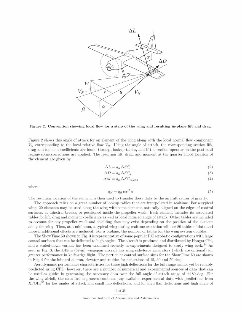
Figure 2. Convention showing local flow for a strip of the wing and resulting in-plane lift and drag.
Figure 2 shows this angle of attack for an element of the wing along with the local normal flow componentVN corresponding to the local relative flow VR. Using the angle of attack, the corresponding section lift,drag and moment coefficients are found through lookup tables, and if the section operates in the post-stallregime some corrections are applied. The resulting lift, drag, and moment at the quarter chord location ofthe element are given by
∆L = qN∆SCl (2)
∆D = qN∆SCd (3)
∆M = qN∆SCm,c/4 (4)
whereqN = qR cos2 β (5)
The resulting location of the element is then used to transfer these data to the aircraft center of gravity.The approach relies on a great number of lookup tables that are interpolated in realtime. For a typical
wing, 20 elements may be used along the wing with some elements naturally aligned on the edges of controlsurfaces, at dihedral breaks, or positioned inside the propeller wash. Each element includes its associatedtables for lift, drag and moment coefficients as well as local induced angle of attack. Other tables are includedto account for any propeller wash and shielding that may exist depending on the position of the elementalong the wing. Thus, at a minimum, a typical wing during realtime execution will use 80 tables of data andmore if additional effects are included. For a biplane, the number of tables for the wing system doubles.
The ShowTime 50 shown in Fig. 3 is representative of some popular RC aerobatic configurations with largecontrol surfaces that can be deflected to high angles. The aircraft is produced and distributed by Hangar 9TM,and a scaled-down variant has been examined recently in experiments designed to study wing rock.34 Asseen in Fig. 3, the 1.45-m (57-in) wingspan aircraft has wing side-force generators (which are optional) forgreater performance in knife-edge flight. The particular control surface sizes for the ShowTime 50 are shownin Fig. 4 for the inboard aileron, elevator and rudder for deflections of 15, 30 and 50 deg.
Aerodynamic performance characteristics for these high deflections for the full range cannot yet be reliablypredicted using CFD; however, there are a number of numerical and experimental sources of data that canbe used as guides in generating the necessary data over the full angle of attack range of ±180 deg. Forthe wing airfoil, the data fusion process combines any available experimental data with predictions fromXFOIL35 for low angles of attack and small flap deflections, and for high flap deflections and high angle of
6 of 35
American Institute of Aeronautics and Astronautics
Figure 3. ShowTime 50 aerobatic RC aircraft configurated with elevator, rudder, ailerons and wing dualside-force generators (graphics rendering by Rick Deltenre).
attack (including reverse flow beyond ±90 deg) semi-empirical techniques are employed to yield results likethose shown in Fig. 5. These particular results are for the ShowTime 50 inboard wing airfoil, but many ofthe trends in the post-stall region are similar across a range of airfoils with differences depending largely onairfoil thickness, camber, control surface size and leading-edge radius. Figures 6 and 7 present the lift anddrag coefficient data as the lift-to-drag (Cl/Cd) ratio and in airfoil polar (Cl-vs-Cd) format, respectively.These are convenient ways of viewing and interpreting the data, and it makes for easy comparison across arange of literature (airfoil data for aircraft, sailing, motorsports, and wind energy). Because the wing airfoilshown in Fig. 4 is symmetrical, the data shown in Figs. 5–7 reflects this fact.
From the known wing geometry and airfoil data as shown, a nonlinear lifting-line code is used to determinethe local induced angle of attack for a given wing angle of attack and control surface deflection. The procedurestarts with an estimated circulation distribution Γi along the wing. From this estimate, the downwashdistribution wi is obtained using Biot-Savart law, and this is used to determine the local lift coefficient Cl
using lookup tables based on data like that shown in Fig. 5. With this lift coefficient and the local geometricproperties, a new estimate for the circulation Γnew is determined. If this new estimate matches the initialvalues within a small, specified tolerance, the solution has converged; otherwise, the iteration continues withunder-relaxation being used to obtain a new estimate for the circulation determined by
Γi+1 = ωΓnew + (1 − ω)Γi (6)
This process is repeated for a 2D sweep over the control surface deflections and angle of attack (nominally−20 deg < α < 20 deg), and the data is saved as a lookup table. During realtime simulation, the inducedangle of attack is tapered to zero at the limits at an absolute angle of attack of 90 deg. Thus, beyond±90 deg, the induced angle of attack is assumed to be zero which is reasonable considering that at 90 degthe wing lift is nearly zero, and beyond this point the aircraft remains in this state (in reverse flow) onlymomentarily while most likely undergoing large angle of attack excursions, e.g., in a tailslide maneuver.
Inboard wingVertical tailHorizontal tail
Figure 4. Airfoil sections used on the ShowTime 50 with control surface deflections of 15, 30 and 50 deg.
7 of 35
American Institute of Aeronautics and Astronautics
Figure 5. Airfoil performance over the full ±180-deg angle of attack range for aileron deflections of 0, ±15, ±30,and ±50 deg.
−180 −135 −90 −45 0 45 90 135 180−60
−40
−20
0
20
40
60
α (deg)
Cl/C
d
Figure 6. Airfoil lift-to-drag characteristics over the full ±180-deg angle of attack range for aileron deflectionsof 0, ±15, ±30, and ±50 deg (see Fig. 5 for legend).
As seen in Fig. 5, around an angle of attack near 90 deg the drag coefficient Cd is ≈ 2 and consistent
8 of 35
American Institute of Aeronautics and Astronautics
Figure 7. Airfoil polar over the ±90-deg angle of attack range for aileron deflections of 0, ±15, ±30, and ±50 deg.
with flat plate theory with corrections that were developed for control surface deflections. For a wing witha moderate aspect ratio, however, the drag coefficient CD at 90 deg is lower than the 2D case,36 thus anadditional correction must be used to take this into account. For a flat plate wing at an angle of attack of90 deg, the pressure on the downstream leeward side is nearly constant because the separated flow cannotsupport a pressure gradient, and this result can be seen in pressure distributions of wind turbine blades at90 deg to the flow.37,38 Consequently, the drag coefficient in the 90-deg case will be nearly constant along theentire wing, and CFD predictions for flat plate wings are consistent with this fact.39 Hence, when the flowis completely separated (beginning after stall), approximately constant pressure on the downstream side ofthe wing is maintained, and as complex as the flow may seem, a 2D assumption and hence the strip theoryapproach can still be used as a model of the flow. This thinking was applied in creating the post-stall 3Dcorrections to the 2D airfoil data.
Figure 8 shows the non-flapped airfoil data for the symmetrical ShowTime 50 airfoil shown in Fig. 5.The data is corrected for 3D post-stall effects as follows. For the 90-deg case alone, various empirical curvefits have been given for the wing drag coefficient CD90
as a function of the wing airfoil drag coefficient Cd90
and wing aspect ratio AR.40 In this development, it is necessary to form a correction that applies not justat 90 deg but over the entire post-stall range of angles of attack. The full-envelope 2D-to-3D correction usedhere begins with a modification of the 90-deg case given by Lindenburg,41 namely
Cd90= 2.2{1 − 0.41[1 − exp(−17/AR)]} (7)
where here the wing aspect ratio AR is used instead of an effective aspect ratio AReff used by Lindenburg.This value Cd90
is simply normalized to provide scaling factor used in the next step, that is
kCd= Cd90
/2.2 (8)
The final drag used for each element of the wing is then given by
Cd,corrected = Cd[1 − w(1 − kCd)] (9)
where w is a cosine weighting function expressed as
w = cos
[
π
(
α− αP,1
αN,2 − αP,1
)
−π
2
]
(10)
where αP,1 and αN,2 define the range over which the correction applies, tapering to zero at the ends. Fur-thermore, to maintain the necessary relationship that CL/CD ≈ 1/ tanα (see Ref. 42), the same correction
9 of 35
American Institute of Aeronautics and Astronautics
Figure 8. Application of post stall correction method for AR = 4.5 showing the uncorrected airfoil data,corrected airfoil data (“3D”), and weighting function w used in the correction for the angle of attack range of0 to 180 deg.
is applied to the local lift coefficient, viz
Cl,corrected = Cl[1 − w(1 − kCd)] (11)
Moreover, since the moment in the post-stall region is driven largely by drag acting on the 50% chord location(the center of pressure), the correction also applies to the moment coefficient, viz
Cm,c/4,corrected = Cm,c/4[1 − w(1 − kCd)] (12)
Figure 8 shows the application of this approach over the range of 0 to 180 deg for the inboard wing airfoillift and drag coefficient data for the zero aileron deflection case that was previously presented in Fig. 5. Theoriginal airfoil data is shown together with the corrected data and the cosine weighting function appliedover the range −25 deg to 160 deg, which approximately defines the post-stall region for this airfoil. Moresophisticated approaches43 could be used for blending in the corrections (via the weighting function, Eq. 10),but the current approach closely models experimental data and has the benefit of being computationallyefficient.
Other important effects modeled include quasi-steady aerodynamics produced by pitch-rate induced airfoilcamber.44,45 A positive pitch rate increases the lift coefficient and moment. Only the pitch-rate effect on liftis discussed here. The effective camber produced by the pitch rate can be approximated from its geometryby
(yc/c)eff = 0.54c
2sin(∆αc/2) (13)
where
∆αc =αc
uR(14)
The pitch-rate increment in section lift coefficient is then obtained from
∆Cl,due to pitch rate = (yc/c)eff
∂Cl
∂(yc/c)(15)
10 of 35
American Institute of Aeronautics and Astronautics
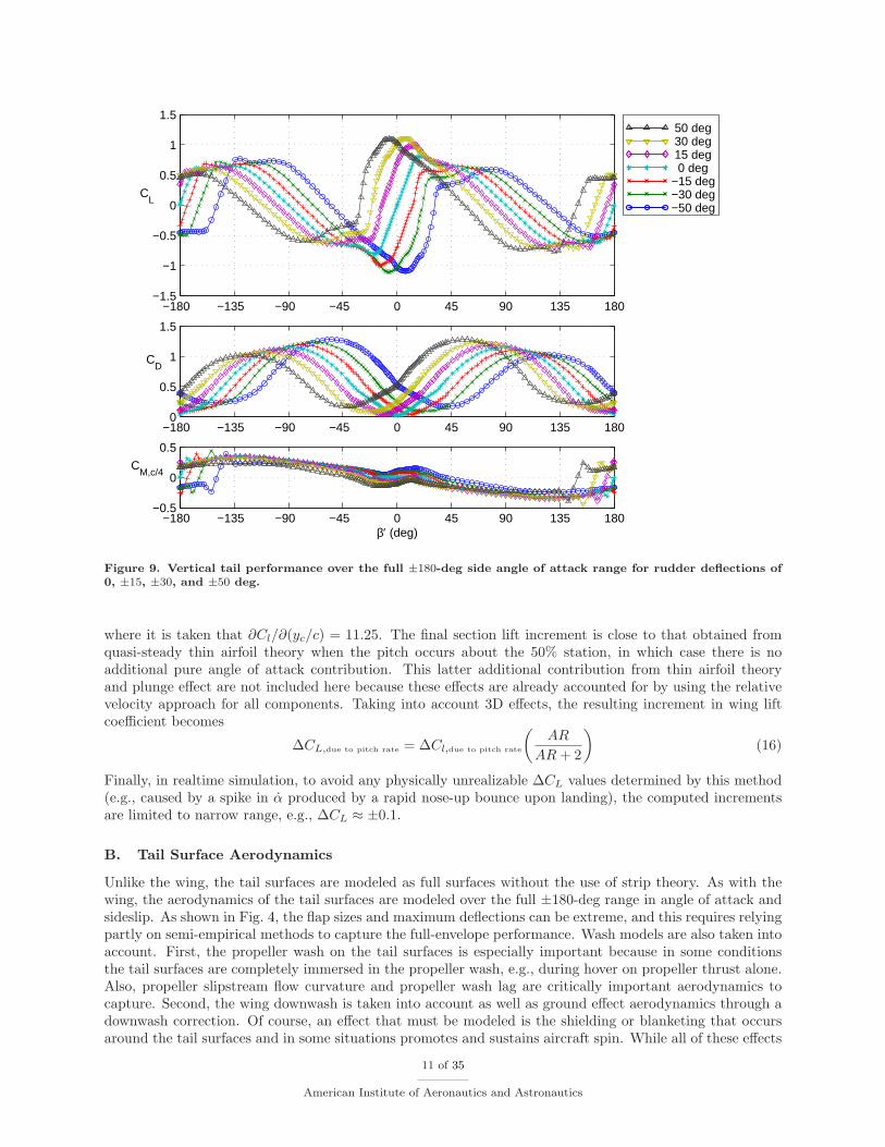
Figure 9. Vertical tail performance over the full ±180-deg side angle of attack range for rudder deflections of0, ±15, ±30, and ±50 deg.
where it is taken that ∂Cl/∂(yc/c) = 11.25. The final section lift increment is close to that obtained fromquasi-steady thin airfoil theory when the pitch occurs about the 50% station, in which case there is noadditional pure angle of attack contribution. This latter additional contribution from thin airfoil theoryand plunge effect are not included here because these effects are already accounted for by using the relativevelocity approach for all components. Taking into account 3D effects, the resulting increment in wing liftcoefficient becomes
∆CL,due to pitch rate = ∆Cl,due to pitch rate
(
AR
AR+ 2
)
(16)
Finally, in realtime simulation, to avoid any physically unrealizable ∆CL values determined by this method(e.g., caused by a spike in α produced by a rapid nose-up bounce upon landing), the computed incrementsare limited to narrow range, e.g., ∆CL ≈ ±0.1.
B. Tail Surface Aerodynamics
Unlike the wing, the tail surfaces are modeled as full surfaces without the use of strip theory. As with thewing, the aerodynamics of the tail surfaces are modeled over the full ±180-deg range in angle of attack andsideslip. As shown in Fig. 4, the flap sizes and maximum deflections can be extreme, and this requires relyingpartly on semi-empirical methods to capture the full-envelope performance. Wash models are also taken intoaccount. First, the propeller wash on the tail surfaces is especially important because in some conditionsthe tail surfaces are completely immersed in the propeller wash, e.g., during hover on propeller thrust alone.Also, propeller slipstream flow curvature and propeller wash lag are critically important aerodynamics tocapture. Second, the wing downwash is taken into account as well as ground effect aerodynamics through adownwash correction. Of course, an effect that must be modeled is the shielding or blanketing that occursaround the tail surfaces and in some situations promotes and sustains aircraft spin. While all of these effects
11 of 35
American Institute of Aeronautics and Astronautics
Figure 10. Vertical tail lift-to-drag characteristics over the full ±180-deg side angle of attack range for rudderdeflections of 0, ±15, ±30, and ±50 deg (see Fig. 9 for legend).
0 0.5 1 1.5−1.5
−1
−0.5
0
0.5
1
1.5
50 deg 30 deg 15 deg 0 deg−15 deg−30 deg−50 deg
CD
CL
Figure 11. Vertical tail polar over the ±90-deg side angle of attack range for rudder deflections of 0, ±15, ±30,and ±50 deg.
and others are modeled in the simulation, not all of these considerations are presented in this paper.
Typically tail surfaces have relatively low aspect ratios, and much data on such wings exists in theliterature, some including flaps and high angle of attack data.45–57 These references were used along withsemi-empirical methods to construct full ±180 deg data. For the vertical fin of the ShowTime 50 model, therudder control surface ratio Sr/S is 0.68, which is extreme (see Fig. 3). Using the methods developed formodeling such surfaces, the data shown in Figs. 9–11 was generated.
The propeller wash on the tail surface begins with the classic momentum theory result58 that the flowthrough the propeller disc is given by
V1 = V∞ + w (17)
where
w =1
2
[
−V∞ +
√
V 2∞ +
(
2T
ρA
)]
(18)
There are a number of additional steps that are considered when extending this basic theory to flow at the tailin the general case of full-envelope flight which can include flight in yawed flow, unsteady aircraft motions,
12 of 35
American Institute of Aeronautics and Astronautics
wake lag effects, and propeller hover and steep descent conditions. These propeller effects are discussed in aseparate companion paper.26
Wing downwash on the horizontal tail is modeled in realtime from the wing lift distribution and thegeometry of the wing relative to the tail. From the lift distribution at any moment in time, the circulationdistribution along the wing is determined. This vorticity is then shed into the wake as discrete filaments,that is, a system of horseshoe vortices that satisfy vortex continuity laws (Helmholtz theorem). The systemincludes vortices trailed from the wing tips and also inboard with alignment on aileron-flap junctures if theyexist. Corrections are applied for wake contraction, angle of attack, sideslip, wall effect and others. Thesewake characteristics are then used to determine the downwash at each tail surface.
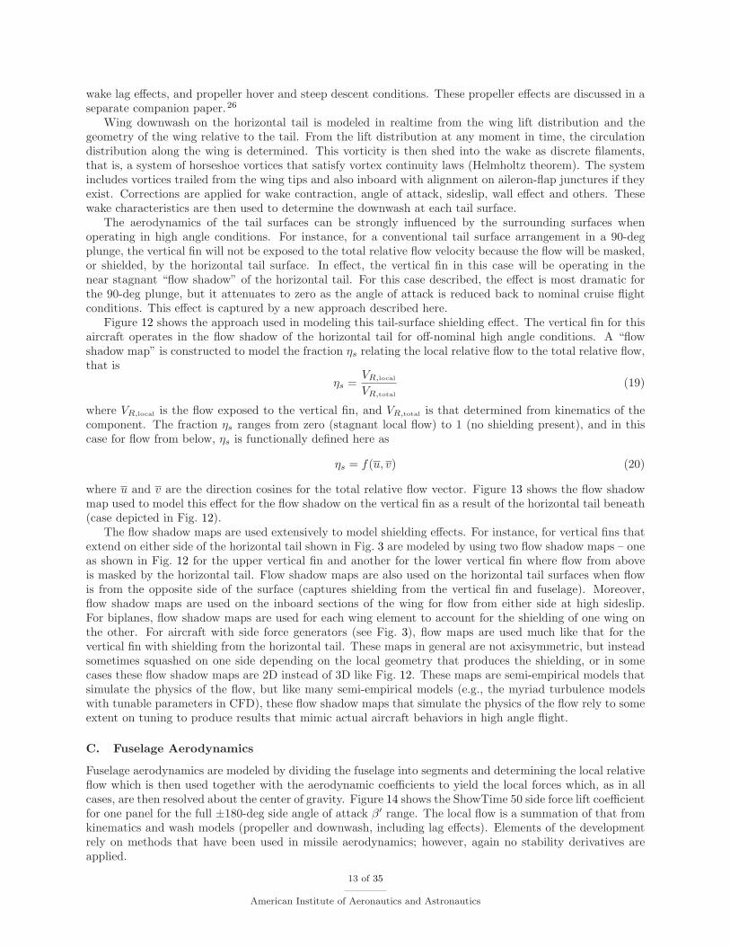
The aerodynamics of the tail surfaces can be strongly influenced by the surrounding surfaces whenoperating in high angle conditions. For instance, for a conventional tail surface arrangement in a 90-degplunge, the vertical fin will not be exposed to the total relative flow velocity because the flow will be masked,or shielded, by the horizontal tail surface. In effect, the vertical fin in this case will be operating in thenear stagnant “flow shadow” of the horizontal tail. For this case described, the effect is most dramatic forthe 90-deg plunge, but it attenuates to zero as the angle of attack is reduced back to nominal cruise flightconditions. This effect is captured by a new approach described here.
Figure 12 shows the approach used in modeling this tail-surface shielding effect. The vertical fin for thisaircraft operates in the flow shadow of the horizontal tail for off-nominal high angle conditions. A “flowshadow map” is constructed to model the fraction ηs relating the local relative flow to the total relative flow,that is
ηs =VR,local
VR,total(19)
where VR,local is the flow exposed to the vertical fin, and VR,total is that determined from kinematics of thecomponent. The fraction ηs ranges from zero (stagnant local flow) to 1 (no shielding present), and in thiscase for flow from below, ηs is functionally defined here as
ηs = f(u, v) (20)
where u and v are the direction cosines for the total relative flow vector. Figure 13 shows the flow shadowmap used to model this effect for the flow shadow on the vertical fin as a result of the horizontal tail beneath(case depicted in Fig. 12).
The flow shadow maps are used extensively to model shielding effects. For instance, for vertical fins thatextend on either side of the horizontal tail shown in Fig. 3 are modeled by using two flow shadow maps – oneas shown in Fig. 12 for the upper vertical fin and another for the lower vertical fin where flow from aboveis masked by the horizontal tail. Flow shadow maps are also used on the horizontal tail surfaces when flowis from the opposite side of the surface (captures shielding from the vertical fin and fuselage). Moreover,flow shadow maps are used on the inboard sections of the wing for flow from either side at high sideslip.For biplanes, flow shadow maps are used for each wing element to account for the shielding of one wing onthe other. For aircraft with side force generators (see Fig. 3), flow maps are used much like that for thevertical fin with shielding from the horizontal tail. These maps in general are not axisymmetric, but insteadsometimes squashed on one side depending on the local geometry that produces the shielding, or in somecases these flow shadow maps are 2D instead of 3D like Fig. 12. These maps are semi-empirical models thatsimulate the physics of the flow, but like many semi-empirical models (e.g., the myriad turbulence modelswith tunable parameters in CFD), these flow shadow maps that simulate the physics of the flow rely to someextent on tuning to produce results that mimic actual aircraft behaviors in high angle flight.
C. Fuselage Aerodynamics
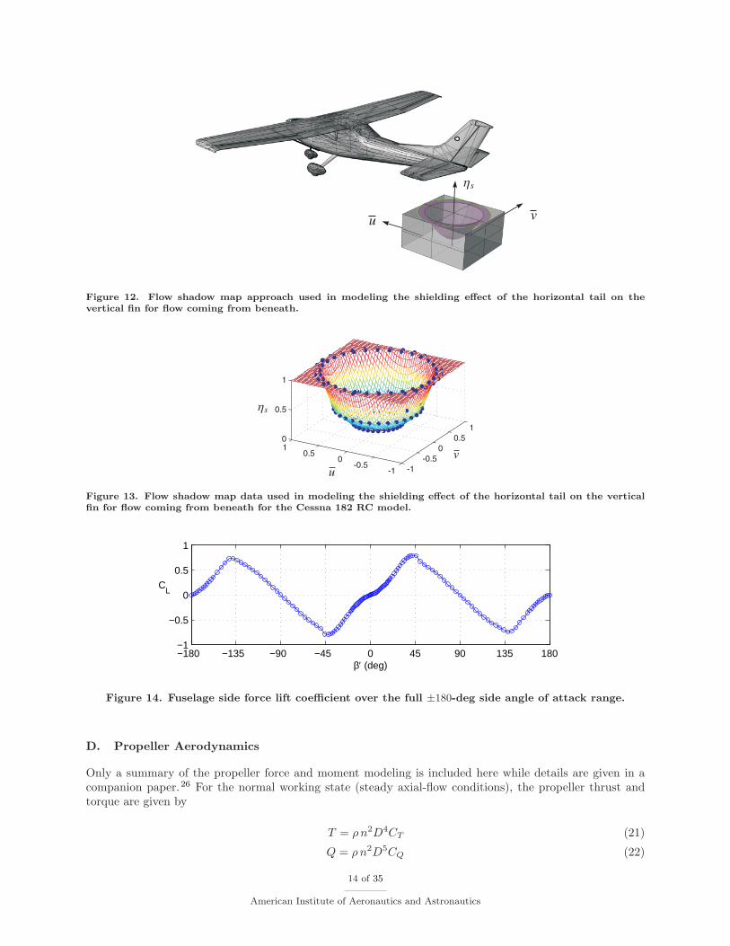
Fuselage aerodynamics are modeled by dividing the fuselage into segments and determining the local relativeflow which is then used together with the aerodynamic coefficients to yield the local forces which, as in allcases, are then resolved about the center of gravity. Figure 14 shows the ShowTime 50 side force lift coefficientfor one panel for the full ±180-deg side angle of attack β′ range. The local flow is a summation of that fromkinematics and wash models (propeller and downwash, including lag effects). Elements of the developmentrely on methods that have been used in missile aerodynamics; however, again no stability derivatives areapplied.
13 of 35
American Institute of Aeronautics and Astronautics
Figure 12. Flow shadow map approach used in modeling the shielding effect of the horizontal tail on thevertical fin for flow coming from beneath.
Figure 13. Flow shadow map data used in modeling the shielding effect of the horizontal tail on the verticalfin for flow coming from beneath for the Cessna 182 RC model.
−180 −135 −90 −45 0 45 90 135 180−1
−0.5
0
0.5
1
β′ (deg)
CL
Figure 14. Fuselage side force lift coefficient over the full ±180-deg side angle of attack range.
D. Propeller Aerodynamics
Only a summary of the propeller force and moment modeling is included here while details are given in acompanion paper.26 For the normal working state (steady axial-flow conditions), the propeller thrust andtorque are given by
T = ρn2D4CT (21)
Q = ρn2D5CQ (22)
14 of 35
American Institute of Aeronautics and Astronautics
where the thrust and torque coefficients are determined through lookup tables on the advance ratio given by
J =VN
nD(23)
In the method, the propeller thrust and torque coefficients are determined from blade element momentumtheory, in particular, using the code PROPID.59–61
Apart from the basic propeller aerodynamics expressed in Eqs. 21 and 22, a number of other factorsmust be considered for any general motion and propeller attitude. These include propeller normal force andP-factor (yawing moment) when the flow is not axial, i.e. when the propeller is at an angle of attack to theflow. These effects are given by58
PN =σqA
2
{
Cl +aJ
2πln
[
1 +
(
π
J
)2]
+π
JCd
}
α (24)
NP =−σqAR
2
{
2π
3JCl +
a
2
[
1 −
(
J
π
)2
ln
(
1 +
[
π
J
]2)]
−π
JCd
}
α (25)
where the average lift coefficient Cl is expressed as
Cl =
(
3J
2π
)[
2
σqA
J
πT + Cd
]
(26)
A number of other significant and important propeller effects are modeled, such as propeller gyroscopicforces, aerodynamic moments from propeller wake swirl on downstream surfaces (wing, fuselage, and tail),propeller wash/tail surface damping effects, and propeller wash lag and wake curvature. The approach tomodeling these effects is described in the companion paper.26
V. Simulation Framework and Validation
The full-envelope aerodynamics modeling methods as described are used in the flight simulator FS One.25
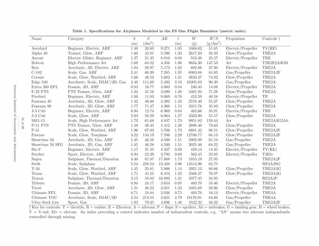
The specific aircraft modeled in the simulator are shown in Table 1, and the same information in Englishunits is given Table 2. The simulation solves the full 6-DOF equations of motion using quaternions, andintegration is carried out using a Runge-Kutta 4-th order scheme running at 300 Hz on a desktop PC. Anefficient interpolation method is incorporated into the code to the extent that upward of 250 tables can beinterpolated in realtime while running the simulation at 300 Hz and rendering the graphics through a typicalPC gaming graphics card at ≈100 Hz or better. The simulator allows for pilot control input through astandard RC transmitter, from any standard USB joystick or from a data file.
The code base is written in C++, is object oriented and includes approximately 600,000 lines of codetogether with 400,000 lines of code (various languages) for aero-physics model development. A large numberof data files for aerodynamics, graphics, ground terrain elevation data, textures, etc. are read at runtimeand make up a substantial part of the overall simulation framework and modeling. The simulator custom-physics engine includes collision detection algorithms between moving aircraft and ground-based objects.“Breakable-parts” physics are also modeled in the simulation to simulate crashes and subsequent missing-part flight dynamics. The simulator has a two-pilot mode where two pilots can fly on one PC using separatepilot controls and split-screen capabilities. Flight dynamics recording features are also embedded in the codeto allow for saving state data to a file which can later be played back as a recording. Recordings can beplayed back as lessons or while actively flying in the simulator in either single-pilot or two-pilot mode.
Wind, the atmospheric boundary layer and turbulence are modeled using a full 3-D turbulent flowfieldenvironment that captures lateral and longitudinal changes along the aircraft extent (wingtip-to-wingtip,nose-to-tail). Tabular turbulence data is generated a priori, read at runtime and used in realtime to obtainthe turbulence quantities for all aircraft components. Also, slope winds and wind shear are modeled andused for slope soaring and dynamic soaring simulation.62
15 of 35
American Institute of Aeronautics and Astronautics
Table 1. Specifications for Airplanes Modeled in the FS One Flight Simulator (metric units).
Name Category b S AR l W W/S Propulsion Controls †(m) (dm2) (m) (g) (g/dm2)
† Key for controls: T = throttle, R = rudder, E = Elevator, A = ailerons, F = flaps, S = spoilers, Ab = airbrakes, G = landing gear, B = wheel brakes,V = V-tail, Elv = elevons. An index preceding a control indicates number of independent controls, e.g. “2A” means two ailerons independentlycontrolled through mixing.
16
of35
Am
erican
Institu
teofA
eronautics
and
Astro
nautics
Table 2. Specifications for Airplanes Modeled in the FS One Flight Simulator (English units).
Name Category b S AR l W W/S Propulsion Controls †(in) (in2) (in) (lb) (oz/ft2)
† Key for controls: T = throttle, R = rudder, E = Elevator, A = ailerons, F = flaps, S = spoilers, Ab = airbrakes, G = landing gear, B = wheel brakes,V = V-tail, Elv = elevons. An index preceding a control indicates number of independent controls, e.g. “2A” means two ailerons independentlycontrolled through mixing.
17
of35
Am
erican
Institu
teofA
eronautics
and
Astro
nautics
−55−50−45−40−35−30−25−20−15−10−5050
5
10
15
−y (m)
−z
(m)
Figure 15. Trajectory of the Extra 260 EFL aerobatic aircraft performing a tailslide [aircraft magnified 2.5times normal size and drawn every 0.55 sec, wingspan of 826 mm (32.5 in)].
The framework described here is the beginning of a new capability for simulation and modeling of full-envelope aircraft flight dynamics. The validation of the approach relies on the validation of the aerodynamicssubsystem component models, which has been accomplished step-by-step for most components described.However, as with any simulation environment, especially in this case involving full-envelope modeling, ele-ments of the simulation must depend to some extent on tuning of parameters to mimic known flight behaviors.Any tuning must result in prescribed data that remains within reasonable physical bounds, such as the ap-proach used here to model the shielding effects at high angles. Where tuning of physical models is used,any of these methods are candidates for refinement by other means as new capabilities become available,e.g. when it is economical to simulate in CFD defined spin states that could be used to advance models foruse in realtime simulations. Finally, in the development of the approach, over 30 aircraft were modeled, andin many cases field tests were performed, recorded on video and used in tuning and refining the methods.Moreover, every airplane in the simulator and hence its underlying models were tested by professional RCpilots (many having more than 30 yrs experience in flying RC models at all levels). The comments by thepilots were in sum that the simulation was very realistic across the broad range of models simulated.
VI. Simulations and Discussion
In this section, flight simulation results of four airplanes performing aerobatic-type maneuvers are dis-cussed. The maneuvers are briefly described using the flight path trajectory and aircraft state data timehistories. Superimposed on the trajectory is a skeleton outline of the aircraft oriented accordingly, and theground trace is shown as a green line. Although the flight dynamics is carried out at 300 Hz, the time historydata is plotted at a rate of 30 Hz, which is the recording rate used for these flights. For several of the flightsdescribed, the maneuver is complex and difficult to ascertain based on these short descriptions and graphicsalone. In these cases, videos of these flights can be viewed online.‡ All of the flights presented here wereperformed by the author, and the results are consistent with observations.
A. Tailslide
The first simulation is a tailslide of the Extra 260 (shown Fig. 1) in longitudinal flight with no control inputsused, and the propeller is static for the duration of the flight. The initial aircraft pitch angle θ is 92 deg,the angle of attack is −178 deg, and the aircraft begins at rest. Figure 15 shows the resulting trajectory inthe y-z plane, and Fig. 16 shows the corresponding time history. As noted in the figure caption, the aircraftis rendered at 2.5 times normal size, and it is drawn every 0.55 sec in this particular case. As the airplanebegins to slide, it is statically unstable in this direction of flight, and thus the nose begins to pitch towardsthe ground (positive q). After 1 sec the airplane flips around nose first. When this happens the followingrapidly occurs: pitch rate peaks, airspeed dips, pitch angle passes through −90 deg and the angle of attackreaches a positive value. Thereafter the gliding airplane zooms and enters the phugoid mode where the angleof attack approaches nearly a constant value before landing.
‡All simulated flights were recorded as videos and are available online at http://www.ae.illinois.edu/m-selig/animations.
18 of 35
American Institute of Aeronautics and Astronautics
Figure 16. Time history of the Extra 260 EFL aerobatic aircraft performing a tailslide (see Fig. 15 fortrajectory).
B. Tailslide with Aileron Input
This next case is the same as before except full left-aileron input (which is opposite that shown in Fig. 1)is used and held constant for the flight. Also, the initial pitch angle is 90 deg. With the flow directly frombehind, the initial angle of attack is 180 deg, and as the airplane falls the flow moves past the 180 deg to−180 deg before flipping around and flying in forward flight. As would be expected, the aircraft in thetailslide first rolls right (positive p) due to reverse flow on the wing, and then after turning around nose firstit rolls left (negative p) as shown in Figs. 17 and 18. When the airplane is released, the initial sideslip anglebegins from a value of 180 deg (relative wind is “in the left ear”), and this value is used in the aerodynamicscalculations. The time history, however, does not show this because the angle plotted is taken from theaircraft state where it is defined per convention to be β = arcsin(v/V ) which is always limited to ±90 deg.
C. Knife Edge Flight
The ShowTime 50 aircraft can be configured with or without wing side force generators (see Fig. 3). Withthe side force generators (SFGs) knife edge flight is enhanced, and this increased performance can be shownin simulation. Figures 19 and 20 are for the ShowTime 50 without SFGs entering a roll and thereaftersustaining knife edge flight with largely right-rudder input. The rudder input is held constant until eventuallythe fuselage stalls in knife edge flight, reaching a sideslip angle of near −65 deg, and rudder input is relievednear 5.5 sec. These same inputs (though truncated in time) were used for the configuration with SFGs, andthe results are shown in Figs. 21 and 22. With SFGs, the aircraft climbs in knife edge flight and initiates aknifed edge loop.
D. High Angle of Attack Flight – Harrier
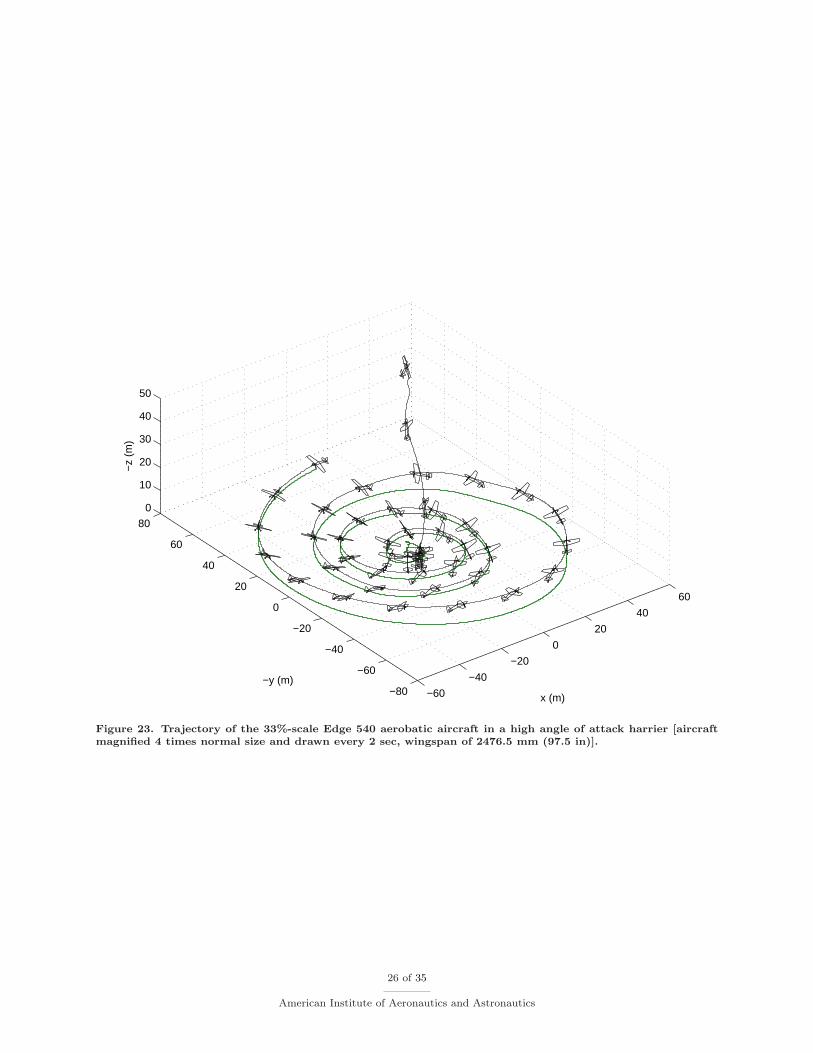
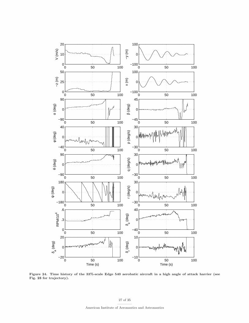
With thrust-to-weight ratios of 2:1, slow flight under power at high angle of attack in the post-stall regimeis possible. In model aviation, this aerobatic maneuver is called a “harrier.” Figures 23 and 24 show a longquasi-steady flight that circles tighter and tighter to a center point where the horizontal speed is ultimatelyarrested, terminating in a vertical exit at the center of the spiral. The aircraft is the 33%-scale Edge 540listed in Table 1 and sketched in Fig. 2.
The flight begins in normal cruise with the angle of attack near 10 deg. As time goes on the up-elevator input is continuously increased. At around 30 sec into the flight, the throttle is advanced because
19 of 35
American Institute of Aeronautics and Astronautics
Figure 17. Trajectory of the Extra 260 EFL aerobatic aircraft performing a tailslide with full left aileron input[aircraft normal size and drawn every 0.2 sec, wingspan of 826 mm (32.5 in)].
the airplane passes from normal flight into the high-drag post-stall regime (around an angle of attack of20 deg). Advancing throttle is required to maintain a height just above ground level. As the flight continues,up-elevator input is increased, the pitch increases, the flight speeds slows, and the throttle is advanced tocounter the increasing drag and loss in wing lift. The resulting slow flight and high pitch are the distinctivehallmarks of a harrier maneuver. This result can be seen in the trajectory where the the pitch increases andthe airplane slows (shorter spacing between aircraft plotted at a time interval of 2 sec). At the center ofthe spiral the airplane is ultimately slowed to a hover position and pointed straight up before advancing thethrottle and climbing out (increasing −z).
E. Upright and Inverted Harrier Sequence
Harriers can be performed upright or inverted, and Figs. 25 and 26 show a flight that includes both for theEdge 540. Apart from the climbing roll at 12 sec (at −y ≈ −50 m in Fig. 25), the aircraft is upright untilapproximately 27 sec into the flight (at −y ≈ 50 m) when the airplane rolls inverted. The transition canbe seen in the angle of attack going from positive to negative and the elevator deflection changing from upelevator to down elevator, which maintains the harrier high angle of attack. What is worth noting are the
20 of 35
American Institute of Aeronautics and Astronautics
Figure 18. Time history of the Extra 260 EFL aerobatic aircraft performing a tailslide with full left aileroninput (see Fig. 17 for trajectory).
accelerations (changes) in roll, pitch, and yaw rates. When upright for the first ≈27 deg, the aircraft is moreunsteady and difficult to fly; whereas, when inverted the excursions are reduced. In real observations, uprightharrier flight of model-scale aircraft are known to wing rock,34 and this characteristic is partly captured bythe simulation as demonstrated here in the time histories.
F. Rolling Harriers
As it sounds, rolling harriers involve rolling flight at slow speeds while maintaining a high angle. The rollis achieved with constant aileron deflection, while the high angle is supported by modulating elevator andrudder input out-of-phase once per roll. As an example, for a left roll, up elevator is used when upright,followed by right rudder when in knife edge. As the roll continues into an inverted attitude, down elevatoris used followed by left rudder when in knife edge. The cycle continues for each harrier roll.
Rolling harriers were simulated using the 46%-scale Ultimate TOC biplane shown in Fig. 27 (see Table 1).Figures 28 and 29 show the rolling harrier maneuver. After takeoff, the left roll starts at 4 sec and ends at
21 of 35
American Institute of Aeronautics and Astronautics
Figure 19. Trajectory of the ShowTime 50 aerobatic aircraft in knife edge flight [aircraft magnified 3 timesnormal size and drawn every 0.5 sec, wingspan of 1448 mm (57 in)].
17 sec as seen in the time history of the roll rate p. During this period of time the aileron input is constantto maintain the constant roll. The high angle is seen in the time histories of the angle of attack and sideslip.These angles modulate out of phase because for the most part the roll is axial with positive pitch θ. Tosustain the high angle, the elevator and rudder are modulated out of phase as seen in their time histories.During the turning part of the trajectory near 10 sec into the flight, the elevator and rudder inputs aremodulated not only out of phase but also biased to the roll angle so that the airplane is turned by theirinputs. Of course, this is difficult to see from the time histories, but in video animation the effect is clearlyvisible. One subtle effect are the slight undulations in the elevation z during the roll. These undulations arecaused by the aircraft falling through the knife edge phases of flight while climbing up during the uprightand inverted harriers phases of the roll. Some skilled professional aerobatic pilots notice this effect andsynchronize throttle burst inputs with the knife edge phases to climb at those points and thus maintaina more constant elevation and thus a more perfect maneuver for visual effect. Finally, it is interesting tosee the total harrier angle (angle of attack and sideslip) start small, grow and then decay. This result is afunction of the total net pilot input (elevator and rudder) that is producing the motion.
G. Inverted Spin – The Blender
The final example here exercises the edges of the aerobatic envelope – the inverted spin. In particular, theentire vertical maneuver from start-to-finish is called the blender, shown in Figs. 30 and 31. From a highaltitude (≈ 340 m) the Ultimate TOC begins a nose down attitude and accelerates along the vertical line atnear 90-deg pitch angle (θ). At 5.7 sec into the flight, a left-aileron pulse input produces a rapid roll rate(p). A fraction of a second after this point, at 6.2 sec, rapid down elevator and right-rudder input causethe airplane to pitch inverted (negative q, increasing θ) and yaw. At this point, the energy in the angularmomentum that was focused around the roll axis (x) is transfer to angular momentum around the yaw axis(z). In the process the total angular momentum is more or less conserved. At just the point where thetransition begins (starts at 6.2 sec), the visual effect is dramatic with the airplane yaw rate peaking and thepitch attitude flattening. Starting at 6.7 sec the aileron input is relieved while the elevator and rudder inputare maintained. The airplane then settles into a steady slow-descent inverted spin at idle throttle setting.As the airplane spins, the heading (ψ) changes continously at a nearly constant rate – 1.46 sec per rotation.
22 of 35
American Institute of Aeronautics and Astronautics
Figure 20. Time history of the ShowTime 50 aerobatic aircraft in knife edge flight (see Fig. 19 for trajectory).
The periodicity can also be seen in the trajectory (Fig. 30) where the interval between aircraft renderingsis 0.365 sec, or once every 90 deg of spin rotation. Once the steady spin develops, the ground trace (greenline in Fig. 30) is nearly circular, and the changes in x and y time histories are thus sinusoidal (see Fig. 31).
23 of 35
American Institute of Aeronautics and Astronautics
Figure 21. Trajectory of the ShowTime 50 SFG aerobatic aircraft in knife edge flight with same input as thatuse in Fig. 19 [aircraft magnified 3 times normal size and drawn every 0.5 sec, wingspan of 1448 mm (57 in)].
Termination of the downline spin begins at 20 sec where rudder input is released followed by advancingthrottle, then corrective opposite aileron input and finally nose-up elevator input before flaring to land atthe pilot station.
VII. Conclusion
This paper shows that complex aerobatic full-envelope maneuvers performed by small ultra-agile RC/UAVconfigurations can be simulated using ±180 deg high-angle data in the component-based approach describedhere. The wings, tail, fuselage, etc. are all modeled separately with corrections applied for any interactions.To capture wide excursions that can occur along the span of the wing, such as in a spin, each wing is subdi-vided into sections and modeled individually, taking into account appropriate downwash effects. It is believedthat this strip theory approach is most likely the best way to capture myriad complex nonlinear aerodynamiceffects in realtime fixed-wing aircraft simulations, and the approximation has many avenues for advancement.The tail surfaces are modeled separately, e.g. right horizontal tail, left horizontal tail, etc. However, eachtail surface component is not subdivided using a lifting-line theory approach but rather modeled as a fullsurface. No stability derivatives are used because it is believed that such an approach is not amenable tomodeling ±180 deg high-angle flight. Rather full aerodynamic coefficients (e.g. Cl, Cd, . . . , CL, CD, . . .) areused. A key element of the current approach involves calculating the local relative flow that takes intoaccount all effects – flight speed, kinematics of the aircraft rotation motions, propeller wash, downwash, andany shielding effects of one surface on another. New approaches to predicting local airfoil section data athigh angle with large control surface deflections are also believed to be key in the success of the method, butthese details are not included in the current paper. This approach in aggregate is able to model challengingproblems in aerodynamics and flight dynamics, including aircraft spin, e.g. as was shown here – the invertedspin of a biplane configuration. The validity of the approach relies on the validity of each sub-model makingup the entire aerodynamics model, and the final results of the simulations are consistent with recorded videoobservations and pilot experience. The approach is readily extended to aircraft of any size, e.g. the approachhas been used to model spin and aerobatic maneuvers of full-scale aircraft. Moreover, the generality of theapproach has been applied to model aircraft with missing, damaged or inoperative parts.
24 of 35
American Institute of Aeronautics and Astronautics
Figure 22. Time history of the ShowTime 50 SFG aerobatic aircraft in knife edge flight with same input asthat use in Fig. 19 (see Fig. 21 for trajectory).
25 of 35
American Institute of Aeronautics and Astronautics
Figure 23. Trajectory of the 33%-scale Edge 540 aerobatic aircraft in a high angle of attack harrier [aircraftmagnified 4 times normal size and drawn every 2 sec, wingspan of 2476.5 mm (97.5 in)].
26 of 35
American Institute of Aeronautics and Astronautics
Figure 25. Trajectory of the 33%-scale Edge 540 aerobatic aircraft in upright and inverted harriers [aircraftmagnified 2 times normal size and drawn every 0.75 sec, wingspan of 2476.5 mm (97.5 in)].
28 of 35
American Institute of Aeronautics and Astronautics
Figure 27. 46%-scale Ultimate TOC biplane used in simulations [rendering taken from simulator, wingspan of2540 mm (100 in)].
−30−20
−100
1020
30
−60
−40
−20
0
20
40
60
0
10
20
x (m)
−y (m)
−z
(m)
Figure 28. Trajectory of the 46%-scale Ultimate TOC aerobatic aircraft performing rolling harriers [aircraftmagnified 2 times normal size and drawn every 0.45 sec, wingspan of 2540 mm (100 in)]
30 of 35
American Institute of Aeronautics and Astronautics
Figure 30. Trajectory of the 46%-scale Ultimate TOC aerobatic aircraft performing a blender / inverted spin[aircraft magnified 2 times normal size and drawn every 0.365 sec, wingspan of 2540 mm (100 in)]
32 of 35
American Institute of Aeronautics and Astronautics
The author would like to thank Brian W. Fuesz and Chris A. Lyon for programming the framework ofthe simulator that includes the methods described in this paper. Also, the aircraft design and developmentgroup at Horizon Hobby is gratefully acknowledged for partly supporting the initial development of thesimulator. The author wishes to acknowledge Pritam P. Sukumar for his efforts in assisting in preparationof some of the plots included in this paper.
References
1Taylor, D. J., OL, M. V., and Cord, T., “SkyTote: An Unmanned Precision Cargo Delivery System,” AIAA Paper2003–2753, July 2003.
2Blauwe, H. D., Bayraktar, S., Feron, E., and Lokumcu, F., “Flight Modeling and Experimental Autonomous HoverControl of a Fixed Wing Mini-UAV at High Angle of Attack,” AIAA Paper 2007–6818, August 2007.
3Frank, A., McGrew, J. S., Valenti, M., Levine, D., and How, J. P., “Hover, Transition, and Level Flight Control Designfor a Single-Propeller Indoor Airplane,” AIAA Paper 2007–6318, August 2007.
4Sobolic, F. M. and How, J. P., “Nonlinear Agile Control Test Bed for a Fixed-Wing Aircraft in a Constrained Environ-ment,” AIAA Paper 2009–1927, April 2009.
5Kubo, D. and Suzuki, S., “Tail-Sitter Vertical Takeoff and Landing Unmanned Aerial Vehicle: Transitional FlightAnalysis,” Journal of Aircraft , Vol. 45, No. 1, 2008, pp. 292–297.
6Stone, R. H., “Aerodynamic Modeling of the Wing-Propeller Interaction for a Tail-Sitter Unmanned Air Vehicle,” Journal
of Aircraft , Vol. 45, No. 1, 2008, pp. 198–210.7Stone, R. H., “Flight Testing of the T-Wing Tail-Sitter Unmanned Air Vehicle,” Journal of Aircraft , Vol. 45, No. 2,
2008, pp. 673–685.8Barlow, J. B., Rae, W. H., Jr., and Pope, A., Low-Speed Wind Tunnel Testing, Third Ed., John Wiley and Sons, New
York, 1999.9Salas, M. D., “Digital Flight: The Last CFD Aeronautical Grand Challenge,” Journal of Scientific Computing, Vol. 28,
No. 213, September 2006, pp. 479–505.10Mavriplis, D. J., Darmofal, D., Keyes, D., and Turner, M., “Petaflops Opportunities for the NASA Fundamental Aero-
nautics Program,” AIAA Paper 2007–4084, June 2007.11Tomac, M. and Rizzi, A., “Creation of Aerodynamic Database for the X-31,” AIAA Paper 2010–501, January 2010.12Ghoreyshi, M., Badcock, K. J., and Woodgate, M. A., “Accelerating the Numerical Generation of Aerodynamic Models
for Flight Simulation,” Journal of Aircraft , Vol. 46, No. 3, May–June 2010, pp. 972–980.13Klein, V. and Morelli, E. A., Aircraft System Identification: Theory and Practice, AIAA Education Series, AIAA,
Reston, VA, 2006.14Jategaonkar, R. V., Flight Vehicle System Identification: A Time Domain Methodology, AIAA Progress in Astronautics
and Aeronautics, AIAA, Reston, VA, 2006.15Tobing, S., Go, T. H., and Vasilescu, R., “Improved Component Buildup Method for Fast Prediction of the Aerodynamic
Performances of a Vertical Takeoff and Landing Micro Air Vehicle,” Computational Fluid Dynamics 2008 , Springer BerlinHeidelberg, 2009, pp. 209–214.
16Guerrero, I., Londenberg, K., Gelhausen, P., and Myklebust, A., “A Powered Lift Aerodynamic Analysis for the Designof Ducted Fan UAVs,” AIAA Paper 2003–6567, September 2003.
17Evans, J. and Nahon, M., “Dynamics Modeling and Performance Evaluation of an Autonomous Underwater Vehicle,”Ocean Engineering, Vol. 31, 2004, pp. 1835–1858.
18Saephan, S. and van Dam, C. P., “Determination of Wing-Only Aircraft Tumbling Characteristics through ComputationalFluid Dynamics,” Journal of Aircraft , Vol. 45, No. 3, May–June 2008, pp. 1044–1053.
19Phillips, W. F., Mechanics of Flight , John Wiley & Sons, New York, 2nd ed., 2010.20Dickes, E. G. and Ralston, J. N., “Application of Large-Angle Data for Flight Simulation,” AIAA Paper 2000–4584,
August 2000.21Foster, J. V., Cunningham, K., Fremaux, C. M., Shah, G. H., Stewart, E. C., Rivers, R. A., Wilborn, J. E., and Gato,
W., “Dynamics Modeling and Simulation of Large Transport Airplanes in Upset Conditions,” AIAA Paper 2005–5933, August2005.
22Gingras, D. R. and Ralston, J. N., “Aerodynamics Modeling for Upset Training,” AIAA Paper 2008–6870, August 2008.23Keller, J. D., McKillip, R. M., Jr., and Wachspress, D. A., “Physical Modeling of Aircraft Upsets for Real-Time Simulation
Applications,” AIAA Paper 2008–6205, August 2008.24Keller, J. D., McKillip, R. M., Jr., and Kim, S., “Aircraft Flight Envelope Determination using Upset Detection and
Physical Modeling Methods,” AIAA Paper 2009–6259, August 2009.25“FS One, Precision RC Flight Simulator,” Software Developed by InertiaSoft, Distributed by Horizon Hobby, Champaign,
IL, 2006.26Selig, M. S., “Modeling Propeller Aerodynamics and Slipstream Effects on Small UAVs in Realtime,” AIAA Paper
2010–7938, August 2010.27Uhlig, D. V., Selig, M. S., and Neogi, N., “Health Monitoring via Neural Networks,” AIAA Paper 2010–3419, April 2010.
34 of 35
American Institute of Aeronautics and Astronautics
28Wright, J. R. and Cooper, J. E., Introduction to Aircraft Aeroelasticity and Loads, Aerospace Series, John Wiley & Sons,England, 2007.
29Johnson, W., Helicopter Theory, Dover, New York, 1980.30McMillan, O. J., Schwind, R. G., Nielsen, J. N., and Dillenius, M. F. E., “Rolling Moments in a Trailing Vortex Flow
Field,” NEAR TR 129, also NASA CR-151961, February 1977.31Poppen, A. P., Jr., “A Method for Estimating the Rolling Moment Due to Spin Rate for Arbitrary Planform Wings,”
NASA TM-86365, January 1985.32Pamadi, B. N. and Taylor, L. W., Jr., “Estimation of Aerodynamic Forces and Moments on a Steadily Spinning Airplane,”
Journal of Aircraft , Vol. 21, No. 12, 1984, pp. 943–954.33Pamadi, B. N., Performance, Stability, Dynamics, and Control of Airplanes, AIAA Education Series, AIAA, Reston,
VA, 1998.34Johnson, B. and Lind, R., “Characterizing Wing Rock with Variations in Size and Configuration of Vertical Tail,” Journal
of Aircraft , Vol. 47, No. 2, March–April 2010, pp. 567–576.35Drela, M., “XFOIL: An Analysis and Design System for Low Reynolds Number Airfoils,” Low Reynolds Number Aero-
dynamics, edited by T. J. Mueller, Vol. 54 of Lecture Notes in Engineering, Springer-Verlag, New York, June 1989, pp. 1–12.36Ostowari, C. and Naik, D., “Post-Stall Wind Tunnel Data for NACA 44XX Series Airfoil Sections,” SERI/STR-217-2559,
January 1985.37Sørensen, N. N., Johansen, J., and Conway, C., “CFD Computations of Wind Turbine Blade Loads During Standstill
Operation KNOW-BLADE,” Risø National Laboratory, Task 3.1 Report, Risø-R-1465(EN), June 2004.38van Rooij, R. P. J. O. M., “Analysis of the Flow Characteristics of Two Nonrotating Rotor Blades,” Journal of Solar
Energy Engineering, Vol. 130, August 2008, 031015 (13 pages).39Sørensen, N. N. and Michelsen, J. A., “Drag Prediction for Blades at High Angle of Attack Using CFD,” Journal of
Solar Energy Engineering, Vol. 126, No. 4, November 2004, pp. 1011–1016, [DOI:10.1115/1.1807854 ].40Spera, D. A., “Models of Lift and Drag Coefficients of Stalled and Unstalled Airfoils in Wind Turbines and Wind
Tunnels,” NASA CR-2008-215434, October 2008.41Lindenburg, C., “Stall Coefficients,” Energy Research Center of the Netherlands, Petten, ECN-RX-01-004, January 2001,
Presented at IEA Symposium on the Aerodynamics of Wind Turbines, National Renewable Energy Laboratory, Golden, CO,December, 2000.
42Tangler, J. L. and Ostowari, C., “Horizontal Axis Wind Turbine Post Stall Airfoil Characteristics Synthesization,”Presented at the Horizontal-Axis Wind Turbine Technology Conference, Cleveland, OH, May, 1984.
43Montgomerie, B., “Methods for Root Effects, Tip Effects and Extending the Angle of Attack Range to ±180 deg, withApplication to Aerodynamics for Blades on Wind Turbines and Propellers,” Swedish Defence Research Agency, FOI-R-1305-SE,ISSN 1650-1942, June 2004.
44Ericsson, L. E., “Vortex Characteristics of Pitching Double-Delta Wings,” Journal of Aircraft , Vol. 36, No. 2, March–April 1999, pp. 349–356.
45Leishman, J. G., Principles of Helicopter Aerodynamics, Cambridge Aerospace Series, Cambridge University Press,Cambridge, 2000.
46Zimmerman, C. H., “Characteristics of Clark Y Airfoils of Small Aspect Ratios,” NACA TR-431, 1933.47Zimmerman, C. H., “Aerodynamic Characteristics of Several Airfoils of Low Aspect Ratio,” NACA TN-539, 1935.48Silverstein, A. and Katzoff, S., “Aerodynamic Characteristics of Horizontal Tail Surfaces,” NACA TR-688, 1940.49Bates, W. R., “Collection and Analysis of Wind-Tunnel Data on the Characteristics of Isolated Tail Surfaces with and
without End Plates ,” NACA TN-1291, 1947.50Whicker, L. F. and Fehlner, L. F., “Free-Stream Characteristics of a Family of Low-Aspect-Ratio, All-Movable Control
Surfaces for Application to Ship Design,” David Taylor Model Basin, Report 933, Washington, DC, December 1958.51Koenig, D. G., “Low-Speed Tests of Semispan-Wing Models at Angles of Attack from 0◦ to 180◦,” NASA MEMO
2-27-59A, April 1959.52Kerwin, J. W., Mandel, P., and Lewis, S. D., “An Experimental Study of a Series of Flapped Rudders,” Journal of Ship
Research, Vol. 16, No. 4, December 1972, pp. 221–239.53Marchaj, C. A., Sail Performance, Adlard Coles Nautical, London, 1996.54Marchaj, C. A., Aero-Hydrodynamics of Sailing, Dodd, Mead & Company, New York, 1979.55Torres, G. and Mueller, T., “Low-Aspect-Ratio Wing Aerodynamics at Low Reynolds Numbers,” AIAA Journal , Vol. 42,
No. 5, May 2004, pp. 865–873.56Desabrais, K. J., “Aerodynamic Forces on an Airdrop Platform,” AIAA Paper 2005–1634, May 2005.57Cosyn, P. and Vierendeels, J., “Numerical Investigation of Low-Aspect-Ratio Wings at Low Reynolds Numbers,” Journal
of Aircraft , Vol. 43, No. 3, May–June 2006, pp. 713–722.58McCormick, B. W., Aerodynamics, Aeronautics, and Flight Mechanics, John Wiley & Sons, New York, 2nd ed., 1995.59Hibbs, B. and Radkey, R. L., “Calculating Rotor Performance with the Revised PROP Computer Code,” Tech. rep.,
Wind Energy Research Center, Rockwell International, Golden, CO, RFP-3508, UC-60, 1983.60Selig, M. S. and Tangler, J. L., “Development and Application of a Multipoint Inverse Design Method for Horizontal
Axis Wind Turbines,” Wind Engineering, Vol. 19, No. 5, 1995, pp. 91–105.61Selig, M. S., “PROPID - Software for Horizontal-Axis Wind Turbine Design and Analysis,”
http://www.ae.illinois.edu/m-selig/propid.html, 1995–.62Sukumar, P. P. and Selig, M. S., “Dynamic Soaring of Sailplanes over Open Fields,” AIAA Paper 2010–4953, June 2010.
35 of 35
American Institute of Aeronautics and Astronautics