MODELING GROUNDWATER-SURFACE WATER INTERACTIONS IN AN OPERATIONAL SETTING BY LINKING RIVERWARE WITH MODFLOW by ALLISON MARIE VALERIO B.S., University of Michigan, 2000 A thesis submitted to the University of Colorado in partial fulfillment of the requirement for the degree of Master of Science Department of Civil, Environmental, and Architectural Engineering 2008
Transcript
MODELING GROUNDWATER-SURFACE WATER INTERACTIONS IN AN
OPERATIONAL SETTING BY LINKING RIVERWARE WITH MODFLOW
by
ALLISON MARIE VALERIO
B.S., University of Michigan, 2000
A thesis submitted to the University of Colorado in partial fulfillment of the
requirement for the degree of
Master of Science
Department of Civil, Environmental, and Architectural Engineering
2008
This thesis entitled: Modeling Groundwater-Surface Water Interactions in an Operational Setting by
Linking RiverWare with MODFLOW written by Allison M. Valerio
has been approved for the Department of Civil, Environmental, and Architectural Engineering
______________________________________________
Harihar Rajaram
______________________________________________
Edith Zagona
______________________________________________
Roseanna Neupauer
Date ____________
The final copy of this thesis has been examined by the signatories, and we Find that both the content and the form meet acceptable presentation standards
Of scholarly work in the above mentioned discipline.
iii
Valerio, Allison (M.S., Civil, Environmental and Architectural Engineering) Modeling Groundwater-Surface Water Interactions in an Operational Setting by Linking RiverWare with MODFLOW Thesis directed by Dr. Edith Zagona and Professor Harihar Rajaram
Accurate representation of groundwater-surface water interactions is
critical to modeling low river flow periods in riparian environments in the semi-arid
southwestern United States. This thesis presents a modeling tool with significant
potential for improved operational decision-making in river reaches influenced by
surface-groundwater interactions.
A link between the object-oriented decision support model RiverWare and the
United States Geological Survey (USGS) quasi three-dimensional finite difference
groundwater flow model MODFLOW was developed. An interactive time stepping
approach is used to link the two models, in which both models run in parallel
exchanging data after each time-step. This linked framework incorporates several
features critical to modeling groundwater-surface interactions in riparian zones,
including riparian evapotranspiration, localized variations in seepage rates, irrigation
return flows and rule-based water allocations to users and/or environmental flows.
The performance of the linked RiverWare-MODFLOW model is illustrated
through applications on the Rio Grande near Albuquerque, New Mexico, where over-
appropriation of human water use adversely impacts the habitat of the endangered Rio
Grande silvery minnow. Improved management practices during low river flow
conditions could prevent channel desiccation and habitat destruction. The linked
model simulations were evaluated against historic data and two current models for the
region. Historic river flows were adequately reproduced by the linked model.
Additionally, an investigation of the linked model’s sensitivity to low river flow
iv
conditions was performed and compared against the two existing regional models. It
was found that the gain/loss between the river and aquifer estimated by the linked
model was not overly sensitive to changes in river flow. In fact, the model produced
similar downstream flows as one of the current models, while displaying less
river/aquifer gain/loss sensitivity to the change in river flow conditions. However,
when compared against the other current model of the region large discrepancies were
apparent in the produced downstream flows. Further analysis revealed that some of
these discrepancies may be attributed to model configuration differences. Overall,
the RiverWare-MODFLOW linked model offers an improved tool for management of
river operations accounting for the relatively rapid groundwater-surface water
interactions in riparian zones.
v
ACKNOWLEDGEMENTS
I wish to extend my gratitude to all persons whom have provided me with
guidance and support. This thesis would not have been possible without you.
In particular, I would like to thank Dr. Edie Zagona and Professor Hari
Rajaram for their continued and consistent commitment to this project. Without their
council and insight I would have been lost. I am truly grateful for your
encouragement.
I would like to thank Nabil Shafike at the New Mexico Interstate Stream
Commission, Mike Roark at the United States Geological Survey, Marc Sidlow at the
U.S. Army Corps of Engineers, and Michael Gabora, for their time, patience, and
models. I would also like to recognize the Albuquerque District U.S. Army Corps of
Engineers and the Albuquerque Area Office of the Bureau of Reclamation for
providing funding for this work.
I would like to acknowledge, Professor Roseanna Neupauer for serving on my
committee and for her grammatical critique of this documentation, thank you.
I would also like to thank Thomas Phillips for his help with ArcGIS and
everyone at CADSWES for their advice and support. The love and reassurance from
my friends and family during the past couple of years has been indispensable to me
and instrumental in my success, thank you all.
Lastly, I would like to thank my husband Joseph Valerio for just being Joe (or
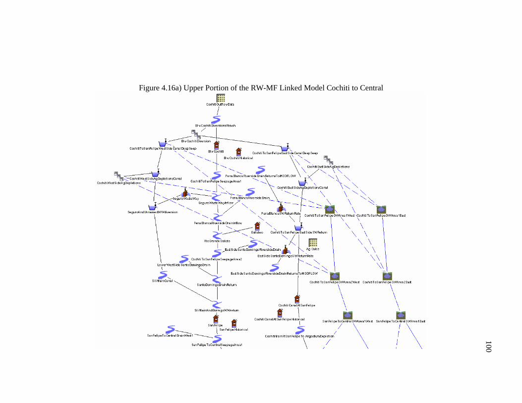
Figure 1.1) Rio Grande Basin ................................................................................... 5 Figure 1.2) Location of the Middle Rio Grande Basin in New Mexico .................... 6 Figure 1.3) Major Physiographic Features of the Middle Rio Grande Basin in New Mexico ........................................................................................... 7 Figure 1.4) Example Depiction of the Middle Rio Grande Irrigation Network ...... 11 Figure 1.5) Rio Grande Silvery Minnow Habitat .................................................... 17 Figure 1.6) Middle Rio Grande Regional Groundwater Model............................... 24 Figure 1.7) URGWOM RiverWare Model .............................................................. 25 Figure 1.8) Riparian Groundwater Models Overlain on the Regional Groundwater Model .............................................................................. 26 Figure 3.1) Plan and Cross Section Views of RiverWare-MODFLOW Interaction ............................................................................................. 49 Figure 3.2) Mapping of MODFLOW Cells to RiverWare Reach and GroundWater Objects for Interpolation and Summation...................... 58 Figure 4.1) Test Model - RiverWare........................................................................ 64 Figure 4.2) Test Model - MODFLOW Model Grid with Stream Segments Marked .................................................................................................. 65 Figure 4.3) Test Model - MODFLOW Model Grid with RiverWare Objects Marked .................................................................................................. 66 Figure 4.4) Test Model - RiverWare with Drain Inflows/Outflows Marked........... 68 Figure 4.5) Upper Albuquerque MODFLOW Model.............................................. 78 Figure 4.6) Cochiti MODFLOW Model.................................................................. 79 Figure 4.7) Rio Grande Below Cochiti Gage Daily Flow Hydrograph 1999-2000 ............................................................................................. 81 Figure 4.8) Rio Grande at San Felipe Gage Daily Flow Hydrograph 1999-2000 ............................................................................................. 82 Figure 4.9) Rio Grande at San Felipe Gage Daily Flow Hydrograph 1999-2000 from RW-MF Linked model .............................................. 82 Figure 4.10) Rio Grande Below Cochiti Gage Daily Flow Hydrograph 1976-1977 ............................................................................................. 86 Figure 4.11) Rio Grande at San Felipe Gage Daily Flow Hydrograph 1976-1977 ............................................................................................. 86 Figure 4.12) Rio Grande Below Cochiti Gage Daily Flow Hydrograph 1984-1985 ............................................................................................. 89 Figure 4.13) Rio Grande at San Felipe Gage Daily Flow Hydrograph 1984-1985 ............................................................................................. 89 Figure 4.14) URGWOM Planning Model Cochiti to Central.................................... 92 Figure 4.15) Upper and Lower Portions of the URGWOM Planning GW Objects Model Cochiti to Central ......................................................... 96 Figure 4.16) Upper and Lower Portions of the RW-MF Linked Model Cochiti to Central................................................................................ 100 Figure 4.17) MODFLOW General Head Boundary Flux/Lateral Boundary Flux for the Upper Portion of the Cochiti to Central Models 1999-2000 ........................................................................................... 106
xi
FIGURES CONTINUED
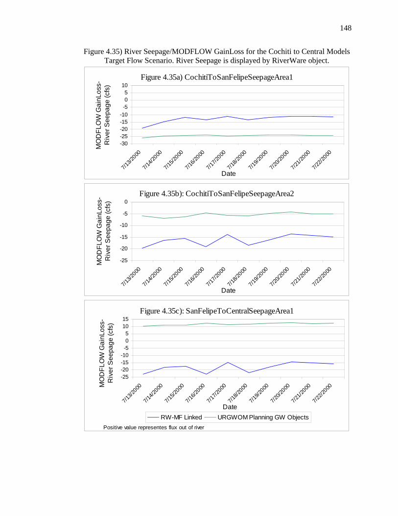
Figure 4.18) MODFLOW General Head Boundary Flux/Lateral Boundary Flux for the Lower Portion of the Cochiti to Central Models 1999-2000 ........................................................................................... 108 Figure 4.19) River Seepage/MODFLOW GainLoss for the Upper Portion of the Cochiti to Central Models 1999-2000........................................... 110 Figure 4.20) River Seepage/MODFLOW GainLoss for the Lower Portion of the Cochiti to Central Models 1999-2000........................................... 111 Figure 4.21) River Seepage/MODFLOW GainLoss Cochiti to Central 1999-2000 ........................................................................................... 112 Figure 4.22) MODFLOW Local Return Flow/RiverWare Drain Inflows for the Cochiti to Central Models 1999-2000................................................. 113 Figure 4.23) Head Difference – Upper Portion of the Cochiti to Central Models 1999-2000 (Cochiti)............................................................................ 115 Figure 4.24) Head Difference – Lower Portion of the Cochiti to Central Models 1999-2000 (UpperAlbuquerque)......................................................... 116 Figure 4.25) Flow at Gages in Cochiti to Central Models for 1999-2000............... 124 Figure 4.26) Flow at Gages in Cochiti to Central Models for 2000 ........................ 126 Figure 4.27) Flow at Below Cochiti Gage in Cochiti to Central Models 1976-1977 ........................................................................................... 133 Figure 4.28) Flow at Cochiti Canal at San Felipe Gage in Cochiti to Central Models 1976-1977 .............................................................................. 134 Figure 4.29) Flow at San Felipe Gage in Cochiti to Central Models 1976-1977 .... 135 Figure 4.30) Flow at Central Gage in Cochiti to Central Models 1976-1977 ......... 136 Figure 4.31) Flow at Gages in Cochiti to Central Models for Artificial Low Flow Scenario...................................................................................... 140 Figure 4.32) River Seepage/MODFLOW GainLoss for the Cochiti to Central Models Artificial Low Flow Scenario ................................................ 142 Figure 4.33) River Seepage/MODFLOW GainLoss for the Cochiti to Central Models Artificial Low Flow Scenario ................................................ 144 Figure 4.34) Flow at Gages in Cochiti to Central Models for Target Flow Scenario............................................................................................... 147 Figure 4.35) River Seepage/MODFLOW GainLoss for the Cochiti to Central Models Target Flow Scenario............................................................. 148 Figure 4.36) River Seepage/MODFLOW GainLoss for the Cochiti to Central Models Target Flow Scenario............................................................. 150 Figure 4.37) Water Balance for Cochiti to Central Models – Water Balance Investigation........................................................................................ 154 Figure 4.38) Flow at Gages in Cochiti to Central Models – Water Balance Investigation........................................................................................ 156 Figure 4.39) Lower Region Diversions Cochiti to Central Models – Water Balance Investigation.......................................................................... 158 Figure 4.40) Canal Inflow at the Top of the Lower Region Cochiti to Central Models – Water Balance Investigation ............................................... 159
xii
FIGURES CONTINUED
Figure 4.41) Lower Region: Total Flow Lost to Canal Seepage and Deep Percolation Cochiti to Central Models – Water Balance Investigation........................................................................................ 160 Figure 4.42) Lower Region: Canal Water Consumed by Irrigation Cochiti to Central Models – Water Balance Investigation ................. 161 Figure 4.43) Lower Region: Flow Remaining in Canal After Irrigation and
Deep Seepage/Percolation Losses Cochiti to Central Models – Water Balance Investigation ............................................................... 161
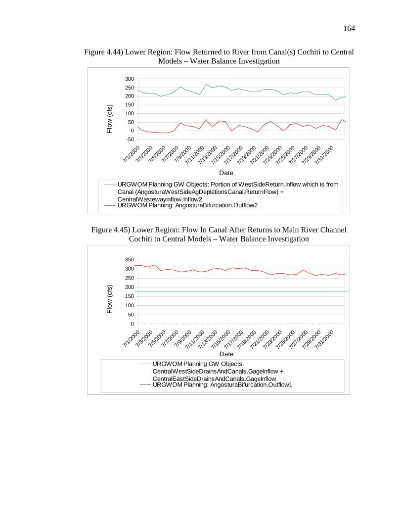
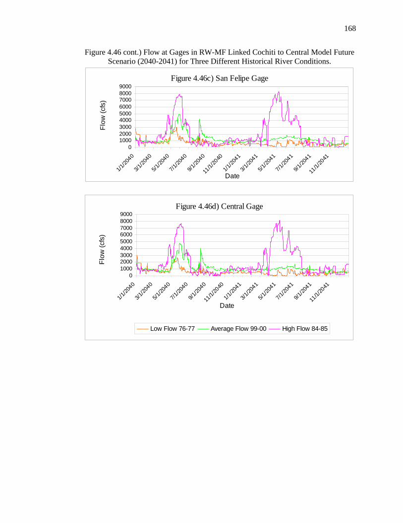
Figure 4.44) Lower Region: Flow Returned to River from Canal(s) Cochiti to Central Models – Water Balance Investigation ................. 164 Figure 4.45) Lower Region: Flow In Canal After Returns to Main River Channel Cochiti to Central Models – Water Balance Investigation .. 164 Figure 4.46) Flow at Gages in RW-MF Linked Cochiti to Central Model Future Scenario (2040-2041) for Three Different Historical River Conditions ................................................................................. 167 Figure 4.47) River Seepage/MODFLOW GainLoss for the RW-MF Linked
Cochiti to Central Model Future Scenario (2040-2041) for Three Different Historical River Conditions................................................. 169
Figure 4.48) River Seepage/MODFLOW GainLoss for the RW-MF Linked Cochiti to Central Model Future Scenario (2040-2041) for Three Different Historical River Conditions................................................. 171
xiii
TABLES
Table 3.1) Data Exchange Summary ........................................................................ 50 Table 4.1) Data Exchanged Between RiverWare and MODFLOW RIV Package............................................................................................. 71 Table 4.2) Data Exchanged Between RiverWare and MODFLOW GHB Package........................................................................................... 73 Table 4.3) Data Exchanged Between RiverWare and MODFLOW STR Package ............................................................................................ 75 Table 4.4) Data Exchanged Between RiverWare and MODFLOW SFR Package ............................................................................................ 75 Table 4.5) RiverWare Object to MODFLOW Cell/Segment Mapping for the Cochiti to Central Case Study RiverWare Models .......................... 102 Table 4.6) Cochiti to Central Models Target Flow Scenario Data Table ............... 151 Table 4.7) Water Balance Investigation Table ....................................................... 155
1
CHAPTER 1 - INTRODUCTION
Interaction between surface water and groundwater is an integral process in
watersheds, governed by climate, geology, surface topology, and ecological factors.
Freeze and Cherry (1979) state a “watershed should be envisaged as a combination of
both the surface drainage area and the parcel of subsurface solid and geologic
formations that underlie it”. However, hydrologic components, such as surface water
and groundwater, have historically been treated as separate units and modeled
accordingly. In the 1960’s the first groundwater surface water interaction studies
focused on the interaction between lakes and groundwater with particular emphasis
on effects related to acid rain and eutrophication (Sophocleous, 2002). By 1970,
groundwater pumping in several regions was found to influence in-stream flows and a
number of studies for conjunctive management of the two resources were conducted
(Barlow and Granato, 2007; and Barlow et al., 2003). More recently, the interaction
between surface water and groundwater along river corridors has received increased
interest due to ecological and climatic concerns (Sophocleous, 2002; S.S.
Papadopulos and Associates and New Mexico Interstate Stream Commission
[NMISC], 2005; Barlow and Granato, 2007).
Many components make up the hydrologic system of a region; accordingly
multiple physical processes must be considered in order to quantify groundwater
surface water interaction along a river corridor such as: overland and in-channel
surface flow; groundwater flow; hyporheic exchange; surface water evaporation; and
riparian evapotranspiration. The extent to which these processes have an effect on a
2
given region depends heavily on the climate, geology, and topography of the region.
In addition to the physical processes, human consumption of available surface water
and groundwater must be considered, especially in arid and semi-arid regions where
supplies are limited and fully appropriated. Strategies for water management
including man-made structures (dams, reservoirs, drains, canals, etc.) add more
complexity to the system. Thus, to adequately quantify groundwater - surface water
interaction, man-made structures and processes such as groundwater withdrawals and
surface water diversions must be taken into account.
The sustainability of human populations and irrigated agriculture in arid
regions, with highly variable climate and surface water flows, is dependent on well
planned management of water resources, which in turn requires a thorough
understanding of the physical processes that govern water movement (Tidwell et al.,
2004; Sallenave and Cowley, 2004). Physical process and operational management
alternatives can be evaluated using hydrologic system models, and in regions where
surface water and groundwater interaction is significant, it is important to be able to
adequately represent the exchange between the two regimes. An example of such an
arid region with an expanding population and widespread agriculture is the Middle
Rio Grande Basin in New Mexico. In this region water managers operate multiple
man-made river structures that provide support for flood control and storage to meet
downstream demands. A couple examples of surface water demands in the region
include irrigation diversions and in-stream flow requirements which sustain
endangered species.
3
To date, the amount of water needed to sustain environmental flows during
times of drought in the Rio Grande Basin has been difficult to predict and the best
strategies for retaining flows have yet to be identified (Cowley, 2006). Here, a better
estimate of flow in the main river channel is needed so that more precise river
operation policies can be developed for low flow conditions. Inadequate estimates of
the interaction between surface and groundwater has been identified as a possible
reason for the poorly predicted flows (Roark, 2007). As such, water managers need a
tool that is able to simulate both the physical processes of flow and management
objectives in order to meet demands. To fulfill this need, a linkage between two
modeling tools, a surface water model RiverWare (Zagona et al., 2001; Zagona et al.,
2005) and a groundwater model MODFLOW (Harbaugh et al., 2000; McDonald and
Harbaugh, 1988) was proposed. This thesis documents the development and testing
of a modeling framework linking RiverWare and MODFLOW, as well as a
description of its application to the Middle Rio Grande.
1.1 Middle Rio Grande Basin Site Background
The Rio Grande flows approximately 1,885 miles, from its headwaters in the
Colorado San Juan Mountains, through New Mexico, Texas, and Mexico before
emptying into the Gulf of Mexico (Kernodle et al., 1987 and United States Geologic
Survey [USGS], 1998). The Rio Grande Basin spans 182,200 square miles and is
divided into multiple subbasins (Figure 1.1). The Middle Rio Grande Basin, one
subbasin of the Rio Grande, is located in central New Mexico (Figures 1.2 and 1.3).
More than 10 million people inhabit the Rio Grande Basin (USGS, 1998) and
approximately 690,000 of them occupy the Middle Rio Grande region (McAda and
4
Barroll, 2002). The Middle Rio Grande Basin encompasses parts of Santa Fe,
Sandoval, Bernalillo, Valencia, Socorro, Torrance, and Cibola Counties with the city
of Albuquerque as the largest population center. Other communities in the Middle
Rio Grande Basin include Rio Rancho, Los Lunas, Belen, Corrales, Bernalillo,
Bernardo, and Isleta (Bartolino and Cole, 2002). In the Middle Rio Grande Basin, a
system of drains and canals spreads laterally away from the river (McAda and
Barroll, 2002). These structures were created to support agriculture (McAda and
Barroll, 2002) and currently there are approximately 55,000 irrigated acres of
agricultural land in the region (Gensler et al., 2007). The location of the Middle Rio
Grande Basin boundaries varies depending on the source quoted. Either the basin
extends from Cochiti to San Acacia or from Cochiti to Elephant Butte. The main
sources (McAda and Barroll, 2002; Thorn et al., 1993; and Kernodle et al., 1995)
referenced in this document define the basin boundaries as Cochiti to San Acacia.
Thus, the use of the term Middle Rio Grande Basin in this document refers to the
region between Cochiti and San Acacia. This region is also sometimes referred to as
the Albuquerque Basin.
5
Figure 1.1) Rio Grande Basin (figure taken from USGS, 1998).
6
Figure 1.2) Location of the Middle Rio Grande Basin in New Mexico (figure taken from McAda and Barroll, 2002).
7
Figure 1.3) Major Physiographic Features of the Middle Rio Grande Basin in New Mexico (figure taken from Bartolino and Cole, 2002).
The Middle Rio Grande Basin is a desert landscape where surface water and
groundwater interaction is of particular interest due to a great degree of water
movement between the two regimes (Bartolino and Cole, 2002). The canals and
drains of the irrigation system, as well as riparian evapotranspiration, have a strong
8
influence on groundwater-surface water interaction in the region (McAda and Barroll,
2002). The following subsections describe the climatic, geologic, hydrologic, and
ecologic features of the Middle Rio Grande Basin. Additionally, summaries of
previously published surface water and groundwater models for the region are
provided.
1.1.1 Climate
Climate in the Middle Rio Grande Basin is semi-arid, with mean annual
precipitation observed from 7.9 to 12.2 centimeters per year, depending on location in
the basin (Dahm et al., 2002). Annual precipitation values of 3.29 to 15.88 inches
(Thorn et al., 1993), with a mean of 8.67 inches (Western Regional Climate Center
[WRCC], 2005) have been recorded for the City of Albuquerque. The mean annual
temperature also varies by location and ranges from 38 to 56 degrees Fahrenheit
(Thorn et al., 1993). The Middle Rio Grande Basin has been defined as a desert and
historically droughts have occurred in the region every 20 to 70 years (Cleverly et al.,
2006). Recent droughts occurred in 1942 -1956, 1976-1977, and 2000-2006. The
predominant surface water supply for the Rio Grande is snowmelt and scattered
summer monsoon thunderstorms (Ward et al., 2006). These recent droughts and
declines of up to 11 percent of mountain snow-pack (as discussed further in
subsection 1.1.5) (New Mexico Drought Task Force, 2006) may be signs of a
predicted drying trend in the region (Seager et al., 2007).
9
1.1.2 Geologic Features
The Middle Rio Grande Basin spans an area of approximately 3,060 square
miles (Figures 1.2 and 1.3). The Middle Rio Grande Basin or depression is one of the
largest basins formed by the Rio Grande Rift. The rift may be described as a set of
North-South trending basins created by crustal extension (Thorn et al., 1993). The
northern boundary of the Middle Rio Grande Basin is defined by the Jemez and
Nacimiento uplifts at an elevation of roughly 6,500 feet above sea level. The Eastern
boundary is defined by the Sandia, Manzano, and Los Pinos uplifts. The Western
boundary, by far the most subdued boundary, is defined by the Rio Puerco Fault Zone
and the Lucero Uplift. The southern boundary of the Basin near San Acacia is
bounded by the convergence of the Eastern and Western boundaries and is at an
elevation of roughly 4,500 feet above sea level (McAda and Barroll, 2002 and Thorn
et al., 1993).
Sedimentary fill in the Middle Rio Grande Basin was deposited as the rift
separated (Thorn et al., 1993). Middle Tertiary to Quaternary Santa Fe Group
sediments constitute the majority of fill in basin and comprise the Santa Fe Aquifer
system. Hawley and Haase (1992) divide the 14,000 thick Santa Fe Aquifer system
into three zones: upper, middle, and lower (McAda and Barroll, 2002). The upper
zone is up to 1,500 feet thick and contains the primary water bearing unit. These
water yielding sediments are marked by intertonguing basin-floor fluvial deposits
(ancestral Rio Grande Channel) and pediment-slope alluvial deposits (Sandia
Mountains) which display anisotropic properties (McAda and Barroll, 2002 and
Thorn et al., 1993).
10
1.1.3 Surface Water Features
The Rio Grande is the fifth largest river in North America. It is a perennial
stream in which some reaches may go dry during years of drought. The Rio Grande
constitutes the greatest surface water inflow to the Middle Rio Grande Basin with an
annual inflow of approximately 1,000,000 acre-feet. The largest tributary to the Rio
Grande in the middle valley is the Jemez River with an average inflow of
approximately 45,000 acre feet, annually. Additional ephemeral tributaries within the
basin include the Santa Fe River, Galisteo Creek, Tijeras Arroyo, Abo Arroyo, Rio
Puerco, and Rio Salado (McAda and Barroll, 2002). The basin is extensively
irrigated. It is estimated that 30 to 40 percent of water consumption is for agriculture
(Shafike, 2008) with the Rio Grande noted as the principal irrigation water source
(McAda and Barroll, 2002). The Middle Rio Grande Conservancy District manages
agricultural water distribution in the basin using a network of 1230 kilometers of
canals, laterals, and ditches (Tidwell et al., 2004).
The Rio Grande valley is wide with a relatively narrow floodplain. Channel
bank stabilization and floodway constriction measures have been implemented to
prevent lateral river migration throughout the basin. Essentially, the natural course of
the river has been restricted, and in the Albuquerque region portions of the river have
become completely disconnected from the historical floodplain (SWCA
Environmental Consultants and New Mexico Interstate Stream Commission
[NMISC], 2007).
Man made river flow management structures in the Middle Rio Grande Basin
include reservoirs, flood retention dams, and a system of irrigation canals and drains.
11
The reservoirs include: Cochiti Lake, Jemez Canyon Reservoir, and Galisteo
Reservoir; the flood retention dams are located near Albuquerque and Rio Rancho;
and the system of irrigation canals and drains span laterally away from the main river
channel (Figure 1.4). River flow is diverted for irrigation at four main points within
the Basin located at Cochiti Dam, Angostura, Isleta, and San Acacia (Figure 1.3). In
addition to natural tributary inflows other sources of inflow (returns) to the main river
channel include: treated wastewater from the cities of Bernalillo, Rio Rancho,
Albuquerque, Los Lunas, and Belen; irrigation diversion return flows; and canal/drain
inflows (see further discussion below) (Bartolino and Cole, 2002).
Figure 1.4) Example Depiction of the Middle Rio Grande Irrigation Network. Riverside drains and irrigation canals are shown (figure taken from Bartolino and
Cole, 2002).
12
In the early 1900’s, leaky unlined irrigation canals, applied irrigation, river
seepage and river channel aggradation from extensive diversion created water-logged
soil conditions in the Rio Grande valley. Interior and riverside drains were installed
along the Rio Grande as part of the solution to mitigate the water logged soils (Thorn
et al., 1993). An example depiction of the drains and canals in the region is shown in
Figure 1.4. When constructed, the drain beds were at an elevation less than the
shallow groundwater heads and were in direct contact with the aquifer. The intent of
the drains was to intercept seepage from the main river channel or leakage in regions
of applied irrigation and/or canals. The drain design allows collected flow to be
returned into the main river channel at a few locations (McAda and Barroll, 2002). In
the past few decades extensive groundwater pumping has led to declining
groundwater levels (S.S. Papadopulos and Associates and NMISC, 2005) and the
elevation of numerous interior drains is now higher than shallow groundwater heads.
Therefore, many interior drains no longer serve their intended purpose. Currently,
during the irrigation season, portions of the riverside drains and some interior drains
are utilized as conveyance channels (McAda and Barroll, 2002).
1.1.4 Groundwater Features
Thorn et al. (1993) describe the Santa Fe Group aquifer system as ranging in
thickness from 2,400 to 14,000 feet, with thickness increasing towards the center of
the basin. The greatest water bearing unit is the upper zone of the Santa Fe Group
which ranges from approximately 1,000 to 1,500 feet in thickness. Up to two-
hundred feet of newer valley fill overlays the Santa Fe Group sediments and functions
as the hydraulic connection between the surface and the Santa Fe Group aquifer
13
(Thorn et al., 1993). These upper 150 to 200 feet of sediments are referred to as the
shallow aquifer (S.S. Papadopulos and Associates and NMISC, 2005) with the
sections beneath referred to as the deep aquifer. Overall groundwater flow is from
the boundaries towards the center of the basin where it trends southwest (McAda and
Barroll, 2002). Within the middle Rio Grande, the two largest rivers, the Rio Grande
and Jemez, are predominantly losing reaches, and thus the main source of recharge to
the aquifer system. However, there are some regions in the basin where the aquifer
discharges to the river. In these reaches surface water and groundwater interaction is
complex and has been difficult to quantify. Additional groundwater recharge and
discharge sources in the basin include canals, irrigated agricultural land,
reservoirs/lakes, subsurface recharge from adjacent basins, precipitation, mountain
front recharge, tributary recharge, and riparian evapotranspiration (McAda and
Barroll, 2002).
Groundwater in the Middle Rio Grande Basin is primarily utilized as a water
source for municipalities and industries. Municipal withdrawal includes well fields
located in the cities of Bernalillo, Rio Rancho, Albuquerque, Bosque Farms, Los
Lunas, and Belen. Additionally, several smaller communities utilize shared well
fields, such as the Mutual Domestic Water Consumers Associations; some pueblos
have well fields; and some single family households have domestic wells. For
industrial use, several corporations have their own wells, with Intel being the largest
consumer of this type (Bartolino and Cole, 2002). By far the city of Albuquerque is
the largest consumer of groundwater (McAda and Barroll, 2002), withdrawing about
100,000 acre-feet annually (Shafike, 2008).
14
1.1.5 Climate Change Concerns
There is increasing concern that anthropogenic climate change will likely have
adverse effects on the available water supply in the Southwestern North America. A
recent study which analyzed multiple climate models predicts that a drying trend in
the American Southwest has already begun and is expected to continue throughout
the century (Seager et al., 2007). Seager et al’s (2007) discussion focused on the rate
of change of precipitation minus evaporation over the region in the various models
which, overall, concluded a decrease in the rate. Future projections are based on
global scale changes in humidity (a humidity increase due to increasing atmospheric
temperatures which reduces moisture divergence over the subtropics) and
atmospheric circulation patterns. In the Rio Grande Basin the climatology record
from 1960 to 2000 was examined, and with moderate-to-strong confidence it was
found that warming is occurring January to March and that spring streamflow has
increased substantially (Hall et al., 2006). In a report compiled by the New Mexico
Office of the State Engineer/Interstate Stream Commission (2006), snowpack in the
Rio Grande Basin was found to be below average for 10 out of 16 years (1990
through 2006). These conditions could be indicative of a possible warming trend.
Panagoulia and Dimou (1996) looked at the sensitivity of groundwater-
streamflow interaction to climate change in a central mountain catchment in Greece
with similar climate as seen in parts of the American Southwest. They utilized a soil
moisture accounting model based on mass balance tracking of percolation and soil
moisture storage coupled with a snow accumulation and ablation model to show that
snowmelt and runoff changes from increasing temperatures had a significant effect on
15
groundwater surface water interaction. They found that increasing temperatures
tended to shift peak water distribution to earlier in the year, for instance to February
instead of April, and that decreased precipitation and increased temperatures
produced lower levels of groundwater storage and streamflow, especially in summer
and fall months. They concluded that surface-groundwater interaction was affected
by temperature changes. In particular, they found that a seasonal shift in snow
accumulation (caused by increased temperatures) yielded a higher groundwater to
stream flow ratio. Observations by Hall et al. (2006) note a shift in spring runoff has
already begun in the northern portions of the Rio Grande Basin, thus this seasonal
shift may have an impact on groundwater surface-water interaction in the Basin. Hall
et al. (2006) also state that seasonal timing and amplitude changes in streamflow
could affect the region both economically and environmentally.
1.1.6 Ecological Concerns
The Rio Grande Silvery Minnow classified in the genus Hybognathus species
amarus (U.S. Fish and Wildlife Service, 2007) was listed as endangered 1994; it is a
pelagic spawner that inhabits the Rio Grande (SWCA Environmental Consultants and
NMISC, 2007) in the 174 mile stretch between Cochiti Reservoir and Elephant Butte
Reservoir, which is approximately 7% of the region it was known to historically
occupy from the confluence of the Rio Chama to the Gulf of Mexico (U.S. Fish and
Wildlife Service, 2007) (Figure 1.5). The Rio Grande silvery minnow once was one
of the most abundant species in the Rio Grande and since being classified as
endangered, the population continued to decline. Its remaining habitat is divided into
four sections by three dams: Angostura Diversion Dam, Isleta Diversion Dam, and
16
San Acacia Diversion Dam (Figure 1.5) (U.S. Fish and Wildlife Service, 2007). The
decreasing silvery minnow population is related to habitat modifications due to the
addition of river management structures (e.g. dams, canals, and levees) which prevent
upstream and downstream movement (U.S. Fish and Wildlife Service, 2002) and have
altered the magnitude and variability of flow including increased and prolonged
desiccation events and decreased peak-flow events. Additionally, during low flow
periods pollutants from municipal and agricultural discharge are found to be elevated
relative to periods of average flow, and these elevated concentrations adversely affect
the Rio Grande silvery minnow. It is found that the Rio Grande silvery minnow tends
to occupy portions of the river that have low to moderate water velocity, and high-
flow events in May or June (e.g. spring runoff and summer storms) trigger it to
release its semi-buoyant, non-adhesive eggs over approximately a three day period.
Spiked releases from Cochiti Reservoir have also been found to trigger spawning
(U.S. Fish and Wildlife Service, 2007). Lack of water has been defined as the “single
most important limiting factor for the survival of the species” (U.S. Fish and Wildlife
Service, 2002). Estimates suggest at least 50 cubic feet per second (cfs) of
streamflow is needed to sustain the species and current federal mandates require 0 to
100 cfs depending on the type of hydrological year in the San Acacia reach (U.S. Fish
and Wildlife Service, 2003). River capsucker, flathead chub, common carp, western
mosquitofish, and red shiner are a few of the 21 native species of fish found in the
New Mexico portion of the Rio Grande. It is estimated that several additional species
have been extirpated from this stretch of the river (SWCA Environmental Consultants
and NMISC, 2007).
17
Figure 1.5) Rio Grande Silvery Minnow Habitat (figure taken from U.S. Fish and Wildlife Service, 2007)
Alterations to natural seasonal flows have had a negative effect on native
species and riparian vegetation throughout the southwestern United States (Cowley,
2006). One example was observed in the Cosumnes River in California where fall
season flows have decreased over the past few decades. These low river flows are a
18
likely contributor to the declining Chinook Salmon population since they occur at the
height of spawning season (Fleckenstein et al., 2004). Fleckenstein et al. (2004)
suggest that low flows are caused by the disconnection of the Cosumnes River and
the underlying aquifer, a common consequence of artificially lowered groundwater
levels (Sophocleous, 2002). Fleckenstein et al. (2004) present several scenarios for
maintaining and/or increasing fall season flows and it was determined that long term
groundwater and surface water management strategies are necessary to improve river
conditions. Their recommendation for an immediate and future increase in fall
season flows combines reduced year round pumping and seasonal surface water
augmentations.
In addition to aquatic species many amphibians, reptiles, mammals, and birds
rely on the Rio Grande and inhabit its riparian corridor (SWCA Environmental
Consultants and NMISC, 2007). Herbaceous and shrubby vegetation predominate the
riverbank ecosystems. Native and non-native invasive species are present including
cottonwood, willow, sleep willow, New Mexico olive, Russian olive and salt cedar
(U.S. Army Corps of Engineers [USACE] et al., 2007). Distribution and composition
of vegetation in these regions is influenced by the quantity of water available.
Shallow groundwater and seepage from the river support these habitats. Over the past
century the density of riparian vegetation has continually increased due to
anthropogenic modifications along the river corridor (Cleverly et al., 2006). Several
researches have estimated the annual uptake of groundwater by riparian
evapotranspiration in the Middle Rio Grande Basin at values ranging from 75,000 to
195,000 acre-feet (McAda and Barroll, 2002), and it has been stated that about two-
19
thirds of the surface water consumption in the basin is from open water surface
evaporation and riparian evapotranspiration (Bartolino and Cole, 2002). Thus,
evapotranspiration constitutes a major component in the water budget of the region.
Seepage from unlined irrigation ditches along the Rio Grande was measured
near Alcalde in Northern New Mexico by Fernald and Guldan (2006), and a
consistent seasonal pattern of elevated shallow groundwater levels were observed
during the irrigation season. They found approximately 5% of flow from the unlined
ditches seeped to the shallow aquifer, except in the near vicinity of the Rio Grande.
In the near vicinity of the Rio Grande (approximately 60 meters from the river)
shallow groundwater levels were less effected by the onset of the irrigation season,
suggesting additional factors such as evapotranspiration and river interaction have a
great influence on shallow aquifer levels in the riparian corridor. In southern New
Mexico between Socorro and San Antonio, river management alternatives have been
tested including the type of riparian vegetation present and alteration of existing
canal/drain system effects on river seepage, with a goal of optimizing Rio Grande
conveyance and in-stream flows (Wilcox et al., 2007). The effects of reduced
riparian evapotranspiration were tested using a MODBRANCH model (see Section
2.1.1.1 for MODBRANCH description). A reduction of 50% from current (year
2000) evapotranspiration rates produced a decrease of approximately 6% of river
seepage, while lesser evapotranspiration reductions of 5% and 20% produced a less
significant decrease to river seepage of 1-2%. Again using a MODBRANCH model
the effects of filling in the LFCC (Low Flow Conveyance Channel) which currently
acts as a riverside drain (no water is diverted into this channel from the river) were
20
tested. River seepage was significantly decreased by the removal of the LFCC (67-
72% reduction), however the desired result of increased water conveyance was not
met and an additional undesired effect of water logged soils downstream was
produced.
1.1.7 River Management
Rio Grande managers are confronted with challenges faced by many arid
regions throughout the world: increasing demands, limited water supplies, and over-
allocation of the existing water supply (Ward et al., 2006). In a system that has fully
appropriated its water, understanding the physical processes that govern its movement
is crucial. The primary goals of river management are daily operations and future
planning including flooding and droughts. Insuring system stability in times of
drought is a high priority and rightly so, with drought occurrence and severity likely
to increase in the region due to a changing climate (Ward et al., 2007).
In New Mexico several state and federal agencies share the responsibility of
managing water resources in the basin: the New Mexico Office of the State Engineer
and Interstate Stream Commission; the Bureau of Reclamation, USACE, and local
Pueblos. Surface water flow in the basin is considered fully appropriated, with the
Rio Grande Compact as the main governing legal contract. The Rio Grande Compact
is a multi-state agreement between Colorado, New Mexico, and Texas for water
allocation. As described in subsection 1.1.3 multiple river management structures
exist along the Rio Grande and coordinated operations are needed to ensure water
demands are met. River managers have used many different modeling schemes to
track and quantify the water budget in the region and a description of existing
21
operational and physical process models, as well as a discussion of economic model
findings for the Basin, are provided below.
Specific surface water management priorities and goals along the Rio Grande
include: flood and sediment control; fish and wildlife enhancement; recreation;
diversion and delivery of irrigation and municipal water; power generation; Native
American water rights; water storage; storage and delivery of San Juan Chama water;
and Rio Grande Compact delivery requirements (U.S. Fish and Wildlife Service,
2008).
1.1.7.1 Middle Rio Grande Operational and Physical Process Models
The USGS has completed multiple reports and several government agencies
have developed groundwater and surface water models of the Rio Grande Basin. For
analyzing groundwater flow in the basin the USGS developed and has continually
updated the Middle Rio Grande Regional Groundwater Model (Kernodle et al., 1987;
Tiedeman et al., 1998; and McAda and Barroll, 2002) (Figure 1.6). The model is
intended as a tool to help water managers quantify available groundwater resources
with in the basin. From here on this model will be referred to as the Regional
Groundwater Model. The Regional Groundwater model uses MODFLOW to model
flow within the Santa Fe Group aquifer and valley fill deposits. MODFLOW is a
three-dimensional, numeric, finite difference, porous medium flow model. At its
core, MODFLOW is a porous medium flow solver which contains several finite-
difference solution methods to the groundwater flow equations. Multiple hydrologic
processes can be incorporated into the basic groundwater flow equations, such as
aquifer withdrawals, surface water gain/loss, and evapotranspiration. The Regional
22
Groundwater model spans from Cochiti to San Acacia and extends up to 9,000 feet in
depth. Nine layers are used which represent changing aquifer properties with well
production predominately from the top five layers. Additionally, several future
projection scenarios have been examined using the Regional Groundwater Model
(Kernodle et al., 1995; Bexfield and McAda 2001; and Bexfield et al., 2004).
For managing surface water in the basin the USACE, Bureau of Reclamation,
USGS, several other federal agencies, and the NMISC have created and maintained
the Upper Rio Grande Water Operations Model (URGWOM) (USACE, 2007)
(Figure 1.7) which is written in the modeling program RiverWare. The URGWOM’s
main functions are long-term planning and evaluation of operations, seasonal
forecasting, and day to day river and reservoir operations, including water accounting.
Current river operations managers use URGWOM to help determine their release and
delivery schedules along the Rio Grande. RiverWare is a surface water object
oriented physical process model that employs user selectable algorithms to represent
each desired physical process. RiverWare is a tool created to help manage basin wide
water allocations in river systems containing management structures (e.g. reservoirs
and diversion dams). RiverWare contains features for: reservoir storage and release
operations; hydropower management; water right and allocation priority rankings (i.e.
law of the river); parameter optimization; and seasonal forecasting. The URGWOM
models the region from Colorado-New Mexico state line to Elephant Butte Reservoir.
While both the URGWOM and Regional Groundwater Model have been in
use for nearly a decade, in the past couple of years a set of riparian-zone groundwater
models were developed by S.S. Papadopulos and Associates and NMISC (2005 and
23
2007). These high resolution MODFLOW models are more refined than the Regional
Groundwater Model and span small sections of the river corridor (Figure 1.8). The
riparian models are similar to the Regional Groundwater Model since they were
created using some of the same data sets as the Regional Groundwater Model and
outputs from the Regional Groundwater Model have been incorporated as boundary
conditions in the Riparian models. These models were developed to evaluate shallow
groundwater conditions in specific river reaches from Cochiti to Elephant Butte
Reservoir for purposes of habitat restoration and river management.
24
Figure 1.6) Middle Rio Grande Regional Groundwater Model (taken from McAda and Barroll, 2002)
25
Figure 1.7) URGWOM RiverWare Model
26
Figure 1.8) Riparian Groundwater Models Overlain on the Regional Groundwater Model. Active model grid is shown for the Regional Groundwater
Model, the full model boundaries are shown for the Cochiti and Upper Albuquerque riparian models in light gray and the active boundaries are shown in dark gray.
27
1.1.7.2 Middle Rio Grande Economic Models
Several studies have been undertaken for regions in the southwestern United
States that address declining flows and forecasted droughts from an economic or cost
network perspective. Ward et al. (2007 and 2006) suggest that water conservation
initiatives tend to be directly linked with the price of water and that economic
damages due to drought conditions could be mitigated by cooperative institutional
water marketing between states. There is a need for models that are able to accurately
incorporate institutional, environmental, and physical processes. Tidwell et al. (2004)
present a planning model that uses systems dynamics or a set of cost-and-effect
relations to model water budget in the Middle Rio Grande region. They found that if
no conservation actions are taken, the rate of groundwater depletion in the basin
increases with time and a deficit accrues when attempting to meet Rio Grande
Compact obligations. While economic models are able to explore water management
alternatives in terms of cost, they are not capable of addressing the physical flow
processes in localized regions to adequately suggest quantities needed to meet flow
targets necessary to protect endangered species and habitat.
1.2 Rationale for Creating the RiverWare-MODFLOW Link
A link between RiverWare (Zagona et al., 2001; Zagona et al., 2005) and
MODFLOW was predicated on the basis that surface water-groundwater interaction
in the Middle Rio Grande Basin have not been adequately addressed by existing
models. The idea stemmed from a need to better predict when and where low flows
will occur along sections of the Rio Grande near Albuquerque, New Mexico. The
28
connection between the river and the aquifer has a significant effect on the quantity of
water in the main channel of the Rio Grande and water managers have had a difficult
time predicting how much water needs to be released from the Cochiti Reservoir in
order to maintain flow in certain sections of the Rio Grande.
The current river operations model (URGWOM) employs the modeling
program RiverWare (see section 1.1.7 for a description of URGWOM and
RiverWare). While RiverWare is a good surface water management tool, it is not well
suited to model the interaction between surface water - groundwater or the small scale
drains and canals present in the basin, due to their small size, large number, and/or
lack of detailed information needed to support these tasks. To rectify this
inadequacy, a proposal was made to link RiverWare with MODFLOW. MODFLOW
was selected for this linkage for several reasons: it is a public domain model; it was
developed so that users with specific needs can easily incorporate new capability into
the system without requiring significant changes to the existing core code; and the
current groundwater flow models for the Rio Grande Basin were constructed using
MODFLOW.
1.3 Linked Model Objective
The basic intent of the linked model is to accurately model a river corridor and
aquifer beneath, including surface water features (e.g. canals, drains, reservoirs) and
surrounding riparian zone, incorporating both natural and human water consumption
from a management perspective. The reasoning behind linking a previously well-
established groundwater model (MODFLOW) with a surface water model
(RiverWare) is to allow each model to handle the processes for which it was
29
designed. It is hoped that by providing water managers with a tool that is able to
simulate both the physical processes of groundwater-surface water flow, water user
demands and associated management objectives, they will be able to adequately
quantify surface flow releases needed during drought periods to meet given
downstream targets.
1.4 Thesis Outline
The following chapters contain a literature review on groundwater-surface
water interaction modeling (Chapter 2), a description of the RiverWare-MODFLOW
Link (Chapter 3), and several Case Studies using the RiverWare-MODFLOW linked
model (Chapter 4), and summary and conclusions (Chapter 5).
30
CHAPTER 2 – LITERATURE REVIEW
The most basic interpretation of surface water-groundwater interaction can be
described by the direction of flux between a surface water body and the underlying
aquifer. Stream reaches may be defined as losing, gaining, or parallel-flow
depending on the elevation difference between stage in the stream and the head in the
aquifer. It should be noted that many in-stream processes are affected by these
interactions such ecological and geochemical processes. However these processes are
beyond the scope of this work and will not be discussed. Instead the reader is
directed to Sophocleous (2002) and Woessner (2000) who provide detailed
descriptions of groundwater surface water interactions and the processes involved,
along with summaries of available literature on the subject.
This chapter focuses on currently available groundwater-surface water
interaction models, a variety of which are available to water resource managers.
Some basic application considerations must be made when selecting an appropriate
model for a project. For instance, what is an acceptable temporal duration and
resolution, spatial dimension, and model solution method (numerical, analytical,
physically based, or data driven)? Various configurations are available for coupling
surface water-groundwater interaction. First, one model could be incorporated into
another or two modeling programs could be run independently. Second, in either
model combination configuration several approaches have been taken to facilitate
data exchange between the two processes (groundwater flow and surface-water flow):
they may be run sequentially with data output from the first process used as input in
31
the second; they may be run in parallel with data exchanged either between time-steps
or by iterative coupling; or they may be intrinsically coupled.
2.1 Coupled Surface Water-Groundwater Models
2.1.1 Physical Process Models
Many of the coupled models discussed in this section model subsurface flow
using MODFLOW, thus a description of this model is provided here. MODFLOW is
a widely used public domain model distributed by the United States Geologic Survey
(USGS). As described in Chapter 1, MODFLOW is a three-dimensional, numeric,
finite difference, porous medium flow model. It contains a porous medium flow
solver with several finite-difference solution methods for the groundwater flow
equations, into which multiple hydrologic processes may be incorporated.
MODFLOW’s formulation allows these hydrologic processes to solve independently
but simultaneously; thus the model is able to represent various combinations of
hydrologic processes at one time. The MODFLOW software was developed to be
adaptable, so users with specific needs would be able to incorporate new capabilities
into its framework without requiring significant changes to the existing core code
(Harbaugh et al., 2000; McDonald and Harbaugh, 1988). Several of the groundwater-
surface water interaction models discussed in this chapter detail user additions to
MODFLOW. Some of these non-standard functions/packages were prepared by the
USGS itself, but were not incorporated into the standard version of MODFLOW.
These include DAFLOW-MODFLOW (Jobson and Harbaugh, 1999) and
MODBRANCH (Swain and Wexler, 1996). The standard MODFLOW 2000 release
does contain several options for modeling surface water features such as lakes,
32
streams, and land-surface recharge and their interaction with the underlying aquifer.
The river/stream packages, STR, SFR, and SFR2 (Prudic, 1989; Prudic et al., 2004;
Niswonger and Prudic, 2005) available in MODFLOW 2000 focus on saturated and
unsaturated flow and route surface channel flow as uniform and steady. The
connection between the stream and aquifer in all three packages is modeled using
Darcy’s Law across the streambed (Prudic, 1989; Prudic et al., 2004; Niswonger and
Prudic, 2005).
2.1.1.1 Groundwater and Surface Channel Flow Models
Two models developed by the USGS, DAFLOW-MODFLOW and
MODBRANCH, employ more advanced channel routing methods than the standard
MODFLOW packages and contain an iterative time stepping approach for coupling
the surface and subsurface interactions. Both models link surface and subsurface
domains using a hydraulic gradient driven flux and assume a saturated subsurface
domain. They both were created from existing surface water routing models and
were restructured and incorporated into MODFLOW. Jobson and Harbaugh’s (1999)
DAFLOW (Diffusion Analogy Surface-Water Flow Model) employs a one
dimensional diffusive wave approximation for in-channel flow while Schaffranek’s
(1987) BRANCH simulates unsteady, non-uniform flow in open channels using an
implicit, weighted four point finite difference approximation for the dynamic wave
equations. BRANCH is referred to as MODBRANCH when incorporated into
MODFLOW (Swain and Wexler, 1996).
In most situations, the temporal scale for modeling groundwater and surface
water systems is intrinsically different - groundwater response is typically modeled
33
on a monthly, seasonal, or yearly time scale while surface water response for
operational purposes is modeled on an hourly, daily or weekly timeframe.
Limitations due to sparse availability of data for groundwater systems is also a time
limiting factor. For example, in the case of Chiew et al. (1992), a monthly time-step
was used for modeling the groundwater system because no data was available to
support a shorter time-step.
Both DAFLOW-MODFLOW and MODBRANCH address the difference
between surface and subsurface modeling time scales using an iterative approach,
whereby the groundwater interval must be an integer multiple of the surface water
time-step. The groundwater head at the beginning and end of a groundwater time-
step is interpolated to obtain a head at the beginning of each surface water time-step
within the interval. For a single groundwater time-step, the surface water and
groundwater routines are repeated until the head and/or stage values compared
between successive iterations fall below a given tolerance.
DAFLOW-MODFLOW was created to simulate flow in upland steams (Jobson and
Harbaugh, 1999) and in their paper Jobson and Harbaugh stated that accuracy
increases with increasing streambed slope. While Lin and Median (2003) use
DAFLOW-MODFLOW in conjunction with MOC3D (a 3-D method-of-
characteristics ground-water flow and transport model integrated in MODFLOW) and
verify contaminant transport results from a tracer test preformed in a mountain
terrain, there are few other published examples which use DAFLOW-MODFLOW.
DAFLOW output is often used in water quality studies as input into BLTM, a
contaminant transport model (Laenen and Risley, 1997; and Broshears et al., 2001).
34
Jobson and Harbaugh do provide several examples in their 1999 report that test the
functionality of the DAFLOW-MODFLOW model. Their scenarios include: stream-
flow resulting from variable recharge; bank storage from flood wave propagation; and
bank storage due to unsteady flow. The first two scenarios use a 7.5 day time-step for
both surface water and groundwater calculations and the third scenario employs
unequal surface and subsurface time-steps with a surface water time-step of 15
minutes and a groundwater time-step that is 30 minutes. From the examples, it
appears that a short time-step on the order of days is appropriate to model the surface
and groundwater interactions using the DAFLOW-MODFLOW model, however this
model is limited in the surface domain features beyond hydraulic routing and is best
suited for modeling steep mountain catchments.
MODBRANCH has been used in several applications, most notably to
examine the effects of raised water levels in the Florida Everglade on a neighboring
residential community in Dade County (Swain et al., 1996). It was also applied in the
Middle Rio Grande Basin to simulate the interaction between surface water and
groundwater in the San Acacia reach (San Acacia to Elephant Butte Reservoir)
(Shafike, 2005). The BRANCH portion of MODBRANCH was used to represent
flow in several proposed canals, where the objective of the canals was to prevent soil
water logging in the residential area. The surface water time-step of 12 hours is an
even multiple of the 5 day groundwater time-step. This model, like DAFLOW-
MODFLOW, is limited in surface water modeling capabilities beyond in-channel
routing, and complex diversion driven operations cannot be represented.
Additionally, MODBRANCH has not been well received by regulatory agencies due
35
to poor performance (Tillery, 2006). Both MODBRANCH and DAFLOW-
MODFLOW are freely available from the USGS.
MODHMS (Hydrogeologic, 1996) goes a step further than DAFLOW-
MODFLOW and MODBRANCH in coupling surface and subsurface flow.
MODHMS is a modified version of MODFLOW that solves a fully three dimensional
saturated/unsaturated subsurface flow equation. Like DAFLOW-MODFLOW,
MODHMS contains a one dimensional diffusive wave approximation for channel
flow. Unlike DAFLOW-MODFLOW, it has an option to solve surface water-
groundwater interactions using a fully implicit procedure and contains a two
dimensional diffusive wave approximation for overland flow and adaptive time
stepping. However, if unequal surface and subsurface timeframes are desired, an
iteratively coupled solution similar to that used in DAFLOW-MODFLOW and
MODBRANCH is employed. MODHMS is not freely available but is distributed by
Hydrogeologic Inc. (Panday and Huyakorn, 2004; and Hydrogeologic, 1996).
MODHMS has been used for large scale basin-wide hydrologic modeling
(Werner et al., 2006; Sedmera et al., 2004). Additionally it has been used to test
management alternatives for water quality control due to seawater intrusion
(Bajracharya et al., 2006; and Werner and Gallagher, 2006; and California Regional
Water Quality Control Board, 2006). The Werner et al. (2006) model employs a
daily time-step for modeling surface features and a monthly time-step for modeling
the subsurface. The other authors did not state what time-step size was used in their
models.
36
Some limitations of the MODHMS model have been identified by the authors
noted above. Werner et al. (2006) ran several scenarios to test MODHMS’s modeling
accuracy and found that when a coarse model scale was used, the model’s ability to
reproduce stream flow processes in the riparian zone was limited. Werner et al.
(2006) and Bajracharya et al. (2006) both encountered numerical errors stemming
from the adaptive time stepping technique. As is the case with MODBRANCH and
DAFLOW-MODFLOW, stream flow management/operation objectives cannot be
represented in MODHMS.
Kollett and Maxwell (2006) present a surface water program coupled with a
variably saturated subsurface system which is similar to MODHMS. They incorporate
a two-dimensional distributed kinematic approximation of overland flow into an
existing model, ParFlow, a parallel three-dimensional finite difference model for
approximating variably saturated groundwater flow. A key difference between
MODHMS and ParFlow is that, in ParFlow, an overland flow boundary condition is
employed instead of a conductance term to bound the interface between surface and
subsurface flow.
Parflow has been used in multiple groundwater modeling applications such as
assessing groundwater level declines in an arid region (Abu-El-Shar’r and Rihani,
2007) and testing of contaminant transport remediation alternatives (Tompson et al.,
1998). However, only one example using Parflow with the overland flow condition
could be found: the Parflow model of Little Washita watershed in Oklahoma
described by Chow et al. (2006) is additionally coupled to an atmospheric model
(APRS). The model was run for a short duration of 48 hours with both surface and
37
subsurface regimes in Parflow using an hourly time-step. Since the authors did not
provide a detailed discussion of the surface/subsurface interaction, no conclusions can
be drawn as to the performance of the model for this process. A drawback of the
Parflow model, as has been previously discussed in terms of the MODLFOW models,
is that surface water management strategies to meet human demands cannot be
incorporated into the model.
2.1.1.2 Groundwater and Watershed Models
Ross et al. (1997) take a different approach to coupling surface and subsurface
flow regimes, in that they look at the surface hydrologic system as a whole and use a
watershed model in lieu of a channel routing model. Their model, the Florida Institute
of Phosphate Research (FIPR) hydrologic model, FHM, simulates the hydrologic
cycle with MODFLOW representing the subsurface domain and Hydrologic
Simulation Program-Fortran (HSPF), a model developed by the Environmental
Protection Agency, representing the surface domain. HSPF is a hydrologic and water
quality model that simulates pervious and impervious surface flow using a lumped
parameter approach. Parameters in the model include overland flow, channel flow,
runoff, aquifer recharge, precipitation, and surface ET. FHM is essentially a shell
program that runs HSPF and MODFLOW and contains a data exchange process
which accommodates spatial and temporal differences between the two models. A
time loop increment is set and the two programs run sequentially. HSPF runs first on
an hourly or shorter basis for one pass through the loop; data is passed to
MODFLOW; and MODFLOW is run for a daily or longer time-step for the same
loop. The looping sequence is repeated until the desired model length is reached.
38
For the coupled models discussed thus far, spatial scale discrepancies
between the surface and subsurface regimes have not needed to be addressed. HSPF
represents the watershed as a collection of subbasins; the spatial extent of each
subbasin is much greater than a single MODFLOW cell - in fact they span large
regions of the MODFLOW domain. The spatial differences between the programs
are handled in a similar fashion as the temporal difference, where data exchange
between the two models is aggregated and disaggregated as necessary. While HSPF
contains methods for tracking flow between surface and unsaturated subsurface
domains, when a continuous simulation is run, flux between the surface and
subsurface is calculated in MODFLOW using the stream or other conductance
concept boundary packages.
FHM was used to evaluate the water budget in the Big Lost River Basin in
Idaho (Said et al., 2005). The surface water - groundwater interaction in the basin are
dynamic; it is noted that precipitation is the main source of groundwater recharge, and
in turn the main water source for the stream is baseflow from the aquifer (Said et al.,
2005). FHM has also been used to model wetland mitigation alternatives and
ecosystem restoration in Saddle Creek in Florida (Tara et al., 2003). The models
presented by Said et al. (2005) and Tara et al. (2003) both employ different time-step
sizes for the surface and groundwater portions of the models. The first uses an hourly
surface water time-step and a daily groundwater time-step, while the latter uses daily
surface water and monthly groundwater time-steps (Said et al., 2005; and Tara et al.,
2003). The FHM model design has multiple limitations including: a total of only
10 diversions can be simulated at one time; the MODFLOW model size must be less
39
than 106 by 60 cells; and all the model simulations involving groundwater-surface
water interaction must be less than one year in length (Ross et al., 1997).
Like FHM, SWAT (Neitsch et al., 2005) is a watershed scale model that
simulates water budget using lumped parameter estimation and has been linked with
MODFLOW to create SWATMOD (Sophocleous and Perkins, 2000). SWAT is a
physically based model which represents a watershed as a group of subbasins.
Lumped hydrologic equations are applied to each subbasin including soil, land use,
and weather data. Alterations were made to MODFLOW’s stream routing package
(STR) to accommodate net surface inflows from SWAT. Spatial differences are a
factor between the two models and a new MODFLOW package was written to
associate data exchange between the SWAT subbbasins and MODFLOW cells.
Additionally, SWAT was modified to accommodate a temporal difference between
SWAT’s daily time-step and larger time-steps on the order of months or a year used
by MODFLOW (Perkins and Sophocleous, 1999; Sophocleous and Perkins, 2000).
SWATMOD uses a time looping procedure similar to that used in FHM.
SWAT has been used mainly for modeling watersheds with a focus on the
impacts of agricultural land use on water supplies, including pollution (Texas Water
Resources Institute, 2007). SWATMOD has been applied to several sites in Kansas
including Rattle Snake Creek and the Lower Republican River Basin (Sophocleous et
al., 1999; and Sophocleous and Perkins, 2000). The goal of both models was to
prevent future declines in the already stressed river system. While SWATMOD is
good for modeling overall water budgeting within a basin the lumped structure of the
surface water portion of the model is not be able to handle individual detailed river
40
diversions, nor can it quantify localized groundwater surface water interaction due to
stream/aquifer flux.
Another linked watershed model, developed by Chiew et al. (1992) employs a
daily rainfall runoff model (Hydrolog) with limited stream routing capabilities.
Hydrolog is integrated with AQUIFEM-N, a quasi three dimensional finite element
model. As with FHM and SWATMOD, spatial and temporal differences exist
between the two flow regimes and are coupled though summation and interpolation.
The Hydrolog-AQUIFEM-N model was used in the Campaspe River Basin in north-
central Australia to estimate fluctuating groundwater recharge. Surface processes
were calculated at a daily time-step and subsurface on a monthly time-step. Like
SWATMOD, Hydrolog-AQUIFEM-N is good for modeling the overall water budget
within a basin, but the lumped structure of the surface water portion of the model
cannot handle multiple river diversions and cannot quantify localized groundwater
surface water interaction.
2.1.2 Operational Models
All the models described above incorporate the physical processes of the
hydrologic cycle and were not designed to handle management and operational
objectives for human demands. Operational management models like RiverWare
were designed to handle management objectives like water allocation. As stated in
Section 1.1.7.1 RiverWare is a surface water object oriented physical process model
that employs user selectable algorithms to represent each desired physical process.
RiverWare is a tool that facilitates management of basin wide water allocations in
river systems containing water management structures (e.g. reservoirs and diversion
41
dams). RiverWare contains features for: reservoir storage and release operations;
hydropower management; water right and allocation priority rankings (i.e. law of the
river); parameter optimization; and seasonal forecasting. Similar to RiverWare,
StateMod, the State of Colorado’s Stream Simulation Model, is a surface water
resources allocation and accounting model. StateMod is capable of modeling
hydrology, water rights, stream management structures (e.g. reservoirs), and
operating rules (State of Colorado, 2004). StateMod is one component of Colorado’s
decision support system (CDSS), a database of hydrologic and administrative
information developed by the Colorado Water Conservation Board and the Colorado
Division of Water Resources (State of Colorado, 2007a). In StateMod a river basin
is represented as a network of connected nodes for which each node represents items
such as stream gauges, diversion structures, and reservoirs. The main components of
the StateMod program include operational rules, return flows, in-stream flows, wells,
base-flows, soil moisture accounting, and diversions. These components combined
can be used for daily operations and future planning (State of Colorado, 2007b).
Models can be set to run at a daily or monthly time-step. Two simplified
groundwater flow mechanisms have been incorporated into StateMod: groundwater
pumping wells and soil moisture accounting. Water from groundwater pumping
wells can be set as inflow sources to surface water features such as diversions and
river flow. Likewise, groundwater sinks such as return flows and river depletions
may be set as surface losses to groundwater. The second feature, soil moisture
accounting, allows for a store of water in the soil zone. The amount of water
available in the soil zone can be controlled using operational rules and can
42
supplement river-base flows (State of Colorado, 2007b). StateMod has been applied
to the Colorado, Gunnison, Yampa, and San Jaun River Basins (State of Colorado,
2007a). The model’s two groundwater features are accounting strategies for
groundwater inflows/outflows to the surface water system and are limited since they
do not model the actual physical process between the two regimes.
The California Water Resources Simulation Model (CalSim) also known as
Water Resources Integrated Modeling System (WRIMS) is a reservoir-river basin
simulation model which employs single time-step optimization (Draper et al., 2004).
It can be used to model operational rules and water allocation by priority ranking.
Like StateMod, CalSim uses a network of connected nodes where each node
represents items (e.g. reservoir) in a stream system. Operational criteria are specified
by weighted priorities within a system of rules and constraints. In CalSim
groundwater is incorporated using a system of interconnected lumped-parameter
basins whose features includes groundwater pumping, irrigation recharge, stream-
aquifer interaction, and inter-basin flow. Draper et al. (2004) state that the
representation of groundwater processes in CalSim is limited. CalSim has been
utilized throughout California in projects such as the Central Valley Project (CVP)
and State Water Project (SWP). The CVP-SWP system models employ a monthly
time-step for applications such as hydrologic behavior, reservoir operations,
hydropower, water quality, and irrigation.
Labadie and Baldo (2000), Fredericks et al. (1998), and Miller et al. (2003)
present MODSIM, a basin-wide and regional river and reservoir operations tool that
employs a minimum cost network flow algorithm satisfying hydrologic mass balance.
43
Like StateMod and CalSim, this surface water management model consists of linked
nodes representing river features such as diversions, inflows, and reservoirs for which
flow distribution can be prioritized to meet management objectives. Interaction of
these features with an underlying aquifer can be incorporated into MODSIM using
response functions generated by MODRSP (Miller et al., 2003) as infiltration and
pumping nodes. The response functions allow transient aquifer recharge conditions
to be incorporated into MODSIM. MODRSP is a modified version of MODFLOW
that generates response functions representing aquifer stresses at each MODFLOW
grid cell. The model was divided into zones based on the output response functions
with each zone containing similar response functions, and each zone is then
correlated to nodes in the MODSIM model.
The MODSIM model with MODRSP response functions has been applied to
several situations involving conjunctive use of surface and groundwater supplies.
The predominant historical use of water in the Snake River Basin was agricultural
irrigation. A desire to increase river stage during low flow seasons to meet
hydroelectricity, recreation, and ecological demands has been expressed (Miller et al.,
2003). Similarly, in the South Platte River Basin increased groundwater pumping
during irrigation season has negatively affected flow in the South Platte River
(Fredericks et al., 1998) and a desire to stabilize and/or increase flows in the river
have been expressed. In order to meet the increased flow demands, the MODSIM
model with MODRSP was used on a monthly time frame to evaluate management
alternatives though increased river diversions for artificial aquifer recharge during
higher flow/less demand periods and their effect on river discharge during low
44
flow/higher demand times (Miller et al., 2003, and Fredericks et al., 1998). While it
was shown in both cases that groundwater recharge augmentation could be tracked
using MODSIM with MODRSP, Miller et al. (2003) admits that that the response
functions cannot be used to quantify riverbed/aquifer flux and both papers agree that
the combined model is best suited for modeling regional basin scales.
While StateMod, CalSim, and MODSIM with MODRSP are good for
modeling large scale surface water operational objectives and contain groundwater
modeling features, none of them are well suited to quantify groundwater-surface
water interaction in localized regions due to the limited scope of their groundwater
features. Thus none of these models would be appropriate to address the
requirements along the Middle Rio Grande.
2.2 Literature Review Findings
The Middle Rio Grande is a desert landscape where surface water and
groundwater interaction is of particular interest due to a great degree of interaction
between the two regimes. In a system that has fully appropriated its water,
understanding the physical processes that govern its movement is crucial. Water
managers must have a tool that is able to simulate both the physical processes of flow
and management objectives in order to meet demands. While multiple models are
available that handle surface water and groundwater interaction, none are able to
incorporate localized physical processes and a complex institutional framework for
water allocation and management.
45
CHAPTER 3 – MODFLOW-RIVERWARE LINK DESCRIPTION
3.1 Introduction
The general framework for coupling RiverWare and MODFLOW is described
in this chapter. This chapter commences with a brief description of the modifications
made to existing RiverWare and MODFLOW codes to facilitate the link (or
coupling). The linked model design is presented using a simplified prototype model
and the chapter concludes with a conspectus on the spatial and temporal variations
between the models.
Throughout the remaining chapters, all RiverWare model objects will be
denoted with bold font and all MODFLOW packages will be denoted in all caps
italics.
3.2 Changes to MODFLOW and RiverWare Models Necessary To
Implement the Link
3.2.1 MODFLOW
MODFLOW 2000 was selected over MODFLOW 2005 because at the
beginning of this undertaking not all standard features available in MODFLOW 2000
were available in MODFLOW 2005. At that time, MODFLOW 2005 was newly
released and had limited capabilities. Selecting MODFLOW 2005 would have
required developers to convert existing models created in MODFLOW 2000 to the
new release. Additionally, it was important to include one non-standard MODFLOW
package, the Riparian Evapotranspiration (RIP-ET) package (Maddock and Baird,
46
2003), which was written into MODFLOW 2000 version 1.15. All modifications
described here were made to the MODFLOW 2000 version 1.15 containing RIP-ET
modifications.
Several MODFLOW subroutines were modified to allow for the MODFLOW
RiverWare coupling. A new MODFLOW FORTRAN library was created and
contains subroutines that are primarily based on MODFLOW’s MAIN procedure,
along with a few additional subroutines. The functionality in the new subroutines and
modified existing subroutines allows RiverWare processes to: start a MODFLOW
computation, advance MODFLOW by one time-step, input data from RiverWare to
MODFLOW, read output data from MODFLOW to be used by RiverWare, and stop a
MODFLOW computation. At this time, a few processes available in MODFLOW
2000 are not supported in the linked model including the Sensitivity (SEN) and
Parameter Estimation (PES) Packages.
3.2.2 RiverWare
As stated previously, RiverWare is an object-oriented, physical process model
for river basins, in which multiple methods are available to represent each process.
RiverWare's Objects represent physical features of the river system such as
reservoirs, river reaches, water users (consumptive use and return flow), diversions,
and shallow groundwater units. Several of RiverWare's existing Objects were
enhanced to accommodate the link with MODFLOW: the Reach, Water User,
Aggregate Diversion Site, and GroundWater objects each contains new methods
that allow an objects’ data to be exchanged with MODFLOW. Essentially, data from
RiverWare that is shared with MODFLOW replaces data that is input by the user in
47
four MODFLOW packages: the General Head Boundary (GHB), River (RIV),
Streamflow-Routing (STR), and updated Streamflow-Routing (SFR). The RiverWare
Computational Subbasin structure was utilized for communication between the
Objects MODFLOW. The role of the Computational Subbasin is described further in
Section 3.3.4.
3.3 System Description with Prototype Model
A description of the linked RiverWare and MODFLOW model is presented
using a prototype RiverWare-MODFLOW interaction. Plan and cross section views
of the prototype are shown in Figure 3.1 and all possible data exchanges are listed in
Table 3.1. Figure 3.1 contains a MODFLOW grid with several surface water features
superimposed on it (bold and dashed black lines), and RiverWare objects designated
as boxes. The model extends across the width of the riparian corridor and all
MODFLOW grid cells shown are considered active. Each data exchange is denoted
with an arrow and is numbered. A few of the data transfers shown (Numbers 8 and 9)
are entirely handled within RiverWare and do not represent an exchange between
RiverWare and MODFLOW and are shown for system illustration purposes.
In the prototype the main river channel is included in both MODFLOW (cells
with square nodes) and RiverWare (boxed Reach object) models. Representing the
river in both RiverWare and MODFLOW affords the following options: multiple
flow routing methods; flow may be subjected to management constraints; and flux
between the river and aquifer may be calculated at a high resolution. Another surface
water feature depicted in the prototype model is a riverside drain/canal: two riverside
drains are shown (dashed black lines) one on either side of the main river channel.
48
The model boundaries are defined using GHB cells in MODFLOW (denoted
with circular markers). These boundary conditions are also incorporated into
RiverWare using the GroundWater object. In the prototype one GroundWater
(GW) object spans all lateral boundary cells in the MODFLOW model.
49
Figue 3.1a) Plan and Cross Section Views of the RiverWare-MODFLOW Interaction – A plan view of a river corridor is shown below containing a main river
channel (bold black lines) and two drains one on either side of the river (dashed lines). A MODFLOW grid is shown with RIV cells denoted with square markers and GHB cells with circular markers, the STR-SFR reaches as the dashed black lines to
the right and left of the river. RiverWare Objects are designated as boxes. Each data exchange is denoted with an arrow and is numbered.
(1) Inflow into riverside drain – in MODFLOW (2) River Stage – to MODFLOW (3) Gain/Loss between river and aquifer – from MODFLOW (4) Diversion from Reach to riverside drain – to MODFLOW (5) Local Inflow/Return Flow from riverside drain to Reach – from MODFLOW (6) GroundWater Head – to MODFLOW (7) Lateral Flux between MODFLOW Lateral Boundary cell and RW GroundWater object head from MODFLOW (8) Diversion from Reach to WaterUser or AggDiversionSite – in RiverWare (9) GroundWater Return Flow – in RiverWare (10) Surface Water Return Flow – to MODFLOW Regional Aquifer Heads – in MODFLOW and RiverWare are input by the user
50
Figue 3.1b) Plan and Cross Section Views of the RiverWare-MODFLOW Interaction - A cross section view of a river corridor is shown below containing a
main river channel and two drains one on either side of the river. A MODFLOW grid is shown with RIV cells denoted with square markers and GHB cells with circular
markers. The STR or SFR package is used to represent the drains these are shown as dips on either side the main river channel. RiverWare Objects are designated as
boxes. Each data exchange is denoted with an arrow and is numbered.
Table 3.1) Data Exchange Summary
Simulation Object Slot
Sum, Interpolation,
or Single Value
MODFLOW Identifier From To
Reach
Total MODFLOW GainLoss
SUM (multiple
cells)
Multiple cells (Layer,Row,
Column) MODFLOW RiverWare
Reach
Inflow Stage and Outflow Stage Interpolation
Multiple cells (Layer,Row,
Column) RiverWare MODFLOW
GroundWater Storage
Lateral Flux from MODFLOW
SUM (multiple
cells)
Multiple cells (Layer,Row,
Column) MODFLOW RiverWare
GroundWater Storage
Previous Elevation Interpolation
Multiple cells (Layer,Row,
Column) RiverWare MODFLOW
Reach
Local Inflow MODFLOW Return Single Value Segment # MODFLOW RiverWare
Reach Diversion Single Value Segment # RiverWare MODFLOW
Water User Surface Return Flow Single Value Segment # RiverWare MODFLOW
AggDiversion Total Surface Return Flow Single Value Segment # RiverWare MODFLOW
51
3.3.1 Main River Channel
In MODFLOW the main river channel is represented using the RIV package
and in RiverWare using a Reach object. The RIV package calculates flow into or out
of a cell from an external source in proportion to the difference between the head in
the cell and the river stage, as shown in the Equations 3.1a) and 3.1b) below
(McDonald and Harbaugh, 1988).
If nkji RBOTh ⟩,, then ( )kjinnn hHRIVCRIVQRIV ,,−= Equation 3.1a
If nkji RBOTh ⟨,, then ( )nnnn RBOTHRIVCRIVQRIV −= Equation 3.1b Where: n is the reach number
nQRIV is the flow between the river and the aquifer, taken as positive if it is directed into the aquifer (L3/T)
nCRIV is the hydraulic conductance of the river-aquifer interconnection (L2/T)
nHRIV is the water level elevation (Stage) in the river (L)
nRBOT is the river bottom elevation (L)
kjih ,, is the head in the cell underlying the river reach (L)
And M
KLWCRIVn = Equation 3.2
Where: K is the riverbed conductivity L is the length of the riverbed W is the width of the riverbed M is the thickness of the riverbed
In RiverWare, the main river channel is represented using a Reach object. In
the linked model, several methods for routing flow are available on the Reach object:
no routing, time lag, variable time lag, and Muskingum Cunge. In addition to the
physical process methods available in RiverWare, Rule-Based Simulation allows for
policy and decision logic to be implemented on river and reservoir operations. For
52
more information about the available routing methods and Rule Based Simulation,
see RiverWare Online Help Documentation (CADSWES, 2007).
As shown in the prototype, the data exchanged between the river and the
aquifer includes stage or river elevation (Figure 3.1 – Number 2) and gain/loss
(Figure 3.1 - Number 3). The river stage elevation as calculated in RiverWare is
transferred to MODFLOW, MODFLOW then calculates the gain/loss between the
main river channel and the shallow groundwater. The purpose of connecting the RIV
package cells with a RiverWare Reach object is to allow the main river channel
calculations, except seepage, to be performed in RiverWare. The RiverWare Reach
object is preferred to the MODFLOW STR and SFR packages for modeling river
operations since policy and decision logic can be applied and RiverWare has more
surface flow routing techniques available.
3.3.2 Riverside or Interior Drain/Canal
A riverside or interior drain or canal may be represented in MODFLOW using
the STR or SFR packages. In STR and SFR packages the continuity equation is used to
route piece-wise steady, uniform, constant-density stream flow (Prudic, 1989 and
Prudic et al., 2004). The STR and SFR packages do not have the capability to
incorporate complex surface water management operation strategies into a
MODFLOW model. Drains/canals typically have few management regulations
governing flow within them. Therefore, the options available in the MODFLOW STR
and SFR packages provide an appropriate representation of these features and thus the
drains/canals would not need to be explicitly represented in RiverWare. Additionally,
drains/canals may have a strong hydraulic connection with the shallow aquifer below,
53
and a high degree of resolution is need to accurately quantify the flux between the
drain/canal and aquifer, and MODFLOW calculations are much better suited for
representing features at high resolution than RiverWare. Since the drain/canal is a
surface water body, an option was added to allow flow between the drain/canal
explicitly represented in MODFLOW and RiverWare surface water bodies. In
MODFLOW’s STR and SFR Packages, stream/river/drain networks are assembled
using reaches and segments. Reaches are joined together to form segments and all
reaches in a segment share the same model properties. A reach can span up to one
model cell, while segments can span multiple cells. Segments are numbered
sequentially starting with the most upstream segment. The reaches in a segment are
also numbered sequentially starting at the most upstream reach.
Four possible exchanges between a drain/canal represented in MODFLOW
and a surface water body represented as a RiverWare object were developed as
described below. For purposes of this discussion a MODFLOW riverside or interior
drain/canal will be referred to as a drain.
1. A diversion from the main river channel to drain is possible (Figure 3.1 – Number
4 and possibly Number 1). This diversion from a RiverWare Reach object is assigned
as inflow into a MODFLOW STR or SFR segment.
2. A return flow from a drain to the main river channel is possible (Figure 3.1 –
Number 5). This return flow diverted from a MODFLOW STR or SFR segment can
be specified as a local inflow into a RiverWare Reach.
54
3. A surface return flow from a WaterUser to a drain is possible (Figure 3.1 –
Number 10). This surface return flow from a RiverWare WaterUser is assigned as
inflow into a MODFLOW STR or SFR segment.
4. A surface return flow from multiple WaterUsers at once to a riverside or interior
drain is possible (Figure 3.1 - Number 10). This surface return flow from a
RiverWare AggDiversion Site is assigned as inflow into a MODFLOW STR or SFR
segment.
3.3.3 Boundary Fluxes
Boundary conditions are a necessary component in a MODFLOW model.
The RiverWare GroundWater object (GW in Figure 3) was modified to incorporate
these boundary conditions into RiverWare and to manage groundwater return flows
from other RiverWare WaterUser objects water users. Several fluxes associated
with boundary conditions are illustrated in the prototype, with only the first pertaining
to a data exchange between RiverWare and MODFLOW (Figure 3.1 – Number 7).
The three remaining fluxes are calculated in RiverWare and accounted for in the
storage equations of the GroundWater objects.
The first flux, which is a lateral boundary flux, is represented in MODFLOW
using the GHB package. Similar to the RIV package, the GHB package simulates flow
into or out of a cell from an external source in proportion to the difference between
the head in the cell and the head assigned to an external source (McDonald and
Harbaugh, 1988). The equation is shown below:
55
( )kjinnn hHBCBQB ,,−= Equation 3.3
Where:
n is the boundary number;
nQB is the flow into cell i,j,k from the boundary, taken as positive if it is directed into the aquifer (L3/T);
nCB is the hydraulic conductance of boundary (L2/T);
nHB is the head elevation (boundary head) assigned to the external source (L);
kjih ,, is the head elevation in cell i,j,k (L)
In this case the external source head is an elevation transferred from RiverWare
(GroundWater object elevation) to MODFLOW (Figure 3.1 – Number 6). Using this
elevation, MODFLOW calculates the flux for each lateral boundary cell. This flux is
then transferred to RiverWare (Figure 3.1 – Number 7) and used in the storage mass
balance equation on the RiverWare GroundWater object LFV in Equation 3.4 below.
GWElevation is the water table elevation in the GroundWater objects’ (L)
( )1−tElevationAdjGW is the adjacent GroundWater objects’ water table elevation at the previous time-step (L); Cond is the conductance between the GroundWater object and the adjacent GroundWater object (L2/T);
( )1−tSGW is the storage on the GroundWater object at the previous time-step (L3);
yS is the specific yield of the GroundWater object;
A is the area of the GroundWater object (L2); The water table elevations in the Groundwater objects are computed from:
( ) ( )AS
tSStElevationElevation
y
GWGWGWGW
11
−−+−= Equation 3.6
Where:
GWElevation is the GroundWater objects’ water table elevation (L);
( )1−tElevationGW is the GroundWater objects’ water table elevation at the previous time-step (L);
GWS is the storage on the GroundWater object (L3);
( )1−tSGW is the storage on the GroundWater object at the previous time-step (L3);
yS is the specific yield of the GroundWater object;
A is the area covered by GroundWater object (L2);
The third flux is a head-based flux PercV between the GroundWater object
and the deep aquifer, which depends on the head difference between them:
PercQ is the flux between the GroundWater object and the Deep Aquifer (L3);
DeepAqCond is the Deep Aquifer Conductance (L3);
( )1−tElevationGW is the water table elevation in the GroundWater object at the previous time-step (L);
( )1−tElevationDeepAq is the head elevation in the Deep Aquifer at the previous time-step (L), shown as Regional Aquifer Head in Figure 3.1;
57
A corresponding deep aquifer boundary should be incorporated into the base layer of
the MODFLOW model using the GHB package. In addition to the fluxes, the
RiverWare GroundWater object accepts return flows from other RiverWare objects,
which are denoted as SWV in Equation 3.4 (Figure 3.1 – Number 9)).
3.3.4 Spatial Considerations of the Linked Model
The conceptual framework of the MODFLOW and RiverWare models are
very different. MODFLOW calculations are performed along a spatial grid, while
RiverWare calculations occur on or between linked objects. Since the model
resolutions may not directly match, some spatial interpolation/summation may be
necessary for data transfer. Since the MODFLOW grid is likely to be at a finer
resolution than the RiverWare objects, a mapping is needed from multiple
MODFLOW cells to a single RiverWare object. Accordingly, spatial interpolation
and summation between some exchanged variables is necessary. This interpolation
and summation is facilitated using the RiverWare Computational Subbasin structure,
in which the user is able to identify which MODFLOW model cells/segments
correspond to a given RiverWare object. Additionally, the linked model framework
allows for multiple MODFLOW models to be associated with a single RiverWare
model. All the objects corresponding with one MODFLOW model are grouped into
single Computational Subbasin. Figure 3.2 presents an example for mapping
MODFLOW cells to RiverWare Groundwater and Reach objects when summation
and interpolation are needed. When a RiverWare Reach is associated with multiple
MODFLOW cells, seepage values are computed for each MODFLOW cell and
58
summed to obtain total seepage over the Reach (Figure 3.2). This seepage is used in
the Reach water balance equation in RiverWare. MODFLOW cells use river stage
values with a higher resolution than RiverWare can provide and stage from the Reach
is therefore interpolated using the computed upstream and downstream values for
each MODFLOW cell, for use in seepage calculation with the RIV package. The
summation and interpolation setup for data exchanged between a GroundWater
object and GHB cells differs from the Reach to RIV cell setup. Because the
GroundWater objects typically represent relatively large regions, elevations from
the GroundWater objects must be interpolated for use in the lateral boundary flux
calculations for GHB cells. Since the GroundWater objects track only one Elevation
(associated with the midpoint of the object), interpolation is needed to represent the
head variation along two adjacent GroundWater objects (Figure 3.2).
Figure 3.2a) Mapping of MODFLOW Cells to RiverWare Reach Object for Interpolation and Summation. RIV cells are denoted with a square marker.
59
Figure 3.2b) Mapping of MODFLOW cells to RiverWare GroundWater object for interpolation and summation. GHB cells are denoted with a circular marker.
3.3.5 Temporal Considerations For The Linked Model
The linked model was designed for regions where groundwater storage
response to changing river conditions is relatively rapid, e.g. on the order of one day.
Therefore, both model components should be run using the same time-step and an
interactive time stepping approach is utilized. RiverWare and MODFLOW run in
parallel exchanging data after each time-step. Essentially, RiverWare and
MODFLOW execute simultaneously. The sequence of operations during a typical
time-step is:
1) RiverWare passes initial conditions to MODFLOW: river stage, groundwater head
elevation, river diversions, water user drain return flows.
2) MODFLOW runs for one time-step and passes appropriate values to RiverWare:
river/aquifer flux, flow in drain/canal, and lateral boundary flux.
60
3) RiverWare runs for the same time-step.
4) Advance to the next time-step. To avoid multiple iterations between the models
during a single time-step, exchanged data may use parameters calculated during the
previous time-step by the other model (explicit coupling).
61
CHAPTER 4 - CASE STUDIES
This chapter contains several model case studies each presented with details
on the model setup and an analysis of the model outputs. The first case study is a
demonstration that the RiverWare-MODFLOW linked model performs all
computations as expected. The second case study shows that, in the absence of river
management operational policy, the RiverWare-MODFLOW linked model performs
similarly to a model run in MODFLOW only. The third case study applies the
RiverWare-MODFLOW model to the Rio Grande near Albuquerque, New Mexico,
and compares its results to two other models of the region as well as historic data.
The fourth case study applies the RiverWare-MODFLOW model to the Rio Grande
near Albuquerque, New Mexico to two different low flow situations: 1) gages in all
three models are compared against one another in an artificial low flow situation;
2) inflow at the most upstream point in the model is determined so that a given target
flow is met at the downstream end of the model. The fifth case study uses the
RiverWare-MODFLOW linked model of the Middle Rio Grande to compare low,
average, and high flow conditions at a future projected scenario. The last section of
this chapter discusses the performance of the RiverWare-MODFLOW model.
All RiverWare model objects are denoted with bold font and all MODFLOW
packages are denoted in all caps italics.
62
4.1 Case Study 1: Demonstration of RiverWare-MODFLOW Link
Functionality
The model described below was used to test the functionality of the
RiveWare-MODFLOW link. Each data exchange in the linked model design is tested
to confirm that it performs as expected. This test model is similar to the prototype
model described in Chapter 3. The test model represents a river corridor containing a
main river channel with two drains, one on either side of main channel. Examples of
movement of water between the surface water features represented in RiverWare and
surface water features represented in MODFLOW are included. There are two
diversions from the main river channel to the drains, two drain outflows into the main
river channel, and two excess surface return flows from water users to the riverside
drains represented in the model.
4.1.1 Description of Test Model
The RiverWare Model contains 6 Reach objects, 11 GroundWater objects,
2 WaterUser objects, and 2 AggDiversionSite objects (Figure 4.1). The Reach
objects model open channel flow. The Reach performs several operations: it can
route flow using several methods (e.g. time lag, Kinematic, and Muskingum); it can
accept outflows and diversions from other objects such as diversions, gains/losses,
and return flows; and it can calculate in-channel flow parameters such as stage and
volume. The GroundWater object is a simple fill-and-spill underground body of
water where the storage and outflow are calculated using a mass balance equation.
Several different configurations of the GroundWater object are possible. In a
RiverWare-MODFLOW linked model the GroundWater objects represent flux
63
between MODFLOW and RiverWare along the model boundaries that represent the
outer edge of the riparian zone. The GroundWater objects can be linked to one
another (Upstream and Downstream) and the flux between objects is head driven.
The GroundWater object can also accept inflows from surface water bodies such as
irrigation groundwater return flows. The WaterUser object simulates the behavior of
a single water user that accepts inflows from other objects. It contains a variety of
methods for calculating the amount of water to be consumed by a given user,
depending on needs of water consumer. It keeps track of the amount of water
delivered to the object (during low flows not all requested water may not be
delivered), and it contains several methods to calculate return flows (i.e. water not
consumed or drained after consumption). The AggDiversion Site object is a
collection of several WaterUser objects. It performs the same calculations as an
individual WaterUser and additionally provides totals over all objects in the set and
allows the user to pick how the objects will solve (lumped, sequentially, etc.).
The MODFLOW model is a rectangular grid of 300 cells, 15 rows by 20
columns, with 20 cells designated as GHB, 30 cells designated as RIV, and 18 STR or
SFR segments defined (Figure 4.2). Two separate MODFLOW models were tested,
one with the drains represented using the STR package and one with the drains
represented using the SFR package. All other inputs in the two MODFLOW models
are identical. In Figures 4.2 and 4.3 the blue cells represent RIV boundary conditions,
the green cells represent GHB boundary conditions, and the pink/purple cells imply
STR or SFR boundary conditions, where the purple cells indicate the beginning of a
MODFLOW STR or SFR segment.
64
Figure 4.1) Test Model - RiverWare
65
Figure 4.2) Test Model - MODFLOW Model Grid with Stream Segments Marked: RIV cells shown in blue, GHB cells are shown in green, cells which are overlain by
STR/SFR segments are shown in pink and purple. The large bold numbers denote the STR/SFR Segment Number.
In Figure 4.2 the stream segment (STR/SFR) numbers are shown with some
cells containing more than one segment. Each Reach object exchanges data with
between four and six MODFLOW RIV cells and each GroundWater object
exchanges data with between two and five MODFLOW GHB cells. Eight of the
MODFLOW STR/SFR segments exchange data with RiverWare, two exchange data
with WaterUser objects, two exchange data with AggDiversionSite objects, and four
exchange data with Reach objects (Figure 4.3 and Figure 4.4).
66
Figure 4.3) Test Model - MODFLOW Model Grid with RiverWare Objects Marked: RIV cells shown in blue, GHB cells are shown in green, cells which are overlain by
STR/SFR segments are shown in pink and purple. The mapping between each RiverWare object and MODFLOW cells is shown. On the RIV cells Reach objects
are denoted in bold with black partitions marking the object boundaries. On the GHB cells GroundWater objects are denoted in bold with the black partitions marking the
division between GroundWater objects for lateral flux summation and the gray partitions marking the division between GroundWater objects for elevation
interpolation. On the STR cells Reach, WaterUser, and AggergateDiversion objects are shown in bold on the cell that exchanges flow with RiverWare.
Figure 4.3 shows a schematic of how the MODFLOW model cells and
segments match up with RiverWare model objects. Figure 4.4 shows a schematic of
the RiverWare model with the data exchanges between surface water bodies in
MODFLOW and in RiverWare marked. For each RiverWare Reach, the stage
interpolation and gain/loss flux summation equations use the same MODFLOW cell
to Reach mapping. Therefore, all blue cells (RIV) between the black dividers are
marked with the matching RiverWare Reach name. For the GroundWater objects,
lateral flux is summed over all cells corresponding to one GroundWater object,
67
while the head is interpolated from between two GroundWater objects. All green
cells (GHB) between the black dividers are summed to obtain the lateral flux for the
indicated GroundWater object. Table 4.2 lists the GroundWater object to GHB cell
mapping for lateral flux interpolation and summation. Heads are interpolated for all
green cells (GHB) between the gray dividers. Table 4.3 shows the MODFLOW STR
to RiverWare object mappings. The MODFLOW segments that exchange data with
RiverWare are set as either tributaries or diversions to/from the main drain segments.
Each of these data exchange segments contain only one reach and are matched with
one RiverWare object. All objects in the RiverWare model were grouped into one
Computational Subbasin called TestSubbasin. All the data exchanged between
RiverWare and MODFLOW is shown for each MODFLOW cell. The RiverWare
object to cell mapping are listed by cell/segment in Tables 4.1 through 4.4.
In the MODFLOW model input files (RIV, GHB and STR/STR), dummy
values were set for variables that receive data from RiverWare. When the data
exchange occurs these dummy values are overwritten with values from RiverWare.
For example, in a RIV cell a stage value is assigned for each stress period in the .riv
input file. The actual stage value used in the calculation is overwritten with a stage
transferred from RiverWare during the simulation.
68
Figure 4.4) Test Model – RiverWare with Drain Inflows/Outflows Marked: The riverside drain inflows/outflows exchanged between the RiverWare and MODFLOW
are marked with a bold arrow and a description of the value exchanged is given.
4.1.2 Test Model Outputs
Data exchanged between the two models can be viewed on the RiverWare
Computational Subbasin. The values shown on the RiverWare Computational
Subbasin are for each individual MODFLOW cell/segment and should correspond to
69
those listed in the MODFLOW output file(s) (.lst or individual output files depending
on the settings selected by the user). The MODFLOW output file (.lst) is structured
by time-step, and contains both inputs and outputs for the RIV, GHB, and STR
packages. It is important to note that the inputs shown in the output file (.lst) may not
reflect the actual value used in the computation. As mentioned previously, a dummy
value must be entered in MODFLOW in order to initiate the MODFLOW run. This
dummy value may appear as the input value in the output file since MODFLOW
writes this portion of the file prior to performing the computations, and thus prior to
RiverWare overwriting the value. All the outputs show in the MODFLOW output
file(s) should correctly match the values shown in RiverWare.
The RiverWare and MODFLOW outputs are presented in
Tables 4.1 though 4.4 for every cell/segment in the Linked Model where data
exchange occurs. A percent difference between the RiverWare and MODFLOW
model outputs is shown and only small rounding errors are noted between the stage,
head, and drain inflow/outflow values extracted from the two models. It is easier to
set RiverWare outputs to contain more digits for precision than MODFLOW outputs.
Thus most of the noted discrepancies are due to lack of precision in the displayed
values in the output file and not the actual values exchanged between the programs.
A good illustration of this discrepancy is to compare the outputs from the STR and
SFR packages; SFR is a newer package than STR and the number of significant
figures included in the output file is greater. Thus the percent differences between the
SFR output and RiverWare output are less than the percent differences between the
STR output and the RiverWare output (Tables 4.3 and 4.4). To verify that the correct
70
stage and head values were transferred from RiverWare and used in MODFLOW, the
last column in each table shows the flux calculated using the RiverWare stage/head
elevation values and the equations employed by MODFLOW. Since these calculated
flux values match well with the outputs from MODFLOW, it can be assumed that the
correct stage/head values were used in the model.
71
Table 4.1a) – Data Exchanged Between RiverWare and MODFLOW RIV Package. Outputs from the RIV Package are listed by MODFLOW cell. The percent difference between MODFLOW (Table 4.1a) and RiverWare (Table 4.1b) Outputs are shown for each
time-step.
71
72
Table 4.1b) – Data Exchanged Between RiverWare and MODFLOW RIV Package. Inputs for the RIV package are listed by MODFLOW cell.
72
73
Table 4.2a) – Data Exchanged Between RiverWare and MODFLOW GHB Package. Outputs from the GHB package listed by MODFLOW cell. The percent difference between MODFLOW (Table 4.2a) and RiverWare (Table 4.2b) Outputs are shown for each
time-step.
73
74
Table 4.2b) – Data Exchanged Between RiverWare and MODFLOW GHB Package. Inputs for the GHB package listed by MODFLOW cell.
74
75
Table 4.3) – Data Exchanged Between RiverWare and MODFLOW STR Package. Outputs for the STR package listed by MODFLOW segment number. The percent difference between MODFLOW and RiverWare Outputs is shown at each time-step.
Table 4.4) – Data Exchanged Between RiverWare and MODFLOW SFR Package. Outputs for the SFR package listed by MODFLOW segment number. The percent difference between MODFLOW and RiverWare Outputs is shown at each time-step.
75
76
4.2 Model Descriptions for Case Studies 2, 3, 4, and 5
Case Studies 2, 3, 4, and 5 include many of the same models with only slight
modifications. In this section a description of each of the models and the variations
between them are provided. All RiverWare model objects are denoted with bold font
and all MODFLOW packages are denoted in all caps italics. The scenarios in case
studies 2, 3, 4, and 5 all simulate 2-year long periods using a daily time-step in both
RiverWare and MODFLOW.
4.2.1 MODFLOW Models
All the MODFLOW models described below are intended to be run while
linked with RiverWare, except for the MFOnly run described in Section 4.2.1.1. The
MFOnly models are MODFLOW model that were used to validate the RiverWare-
MODFLOW linked model.
4.2.1.1 Cochiti to Central 1999-2000
Two MODFLOW groundwater models, Upper Albuquerque Riparian Model
(S.S. Papadopulos and Associates and NMISC, 2005) (Figure 4.5) and Cochiti
Riparian Model (S.S. Papadopulos and Associates and NMISC, 2007) (Figure 4.6),
provided by the NMISC required minor changes to accommodate a link with
RiverWare. The Cochiti MODFLOW Model covers the region from south of the
Cochiti Reservoir to the Angostura Diversion Dam, and the Upper Albuquerque
MODFLOW Model covers the region from Angostura Diversion Dam to Central
Avenue just south of I-40. Data included in the models support a run for the years
1999-2000. Both Riparian models use 125 by 250 foot grid cells with their axis
77
aligned lengthwise along the river. The model grids contain 122 columns by
444 rows (Cochiti) and 255 columns by 458 rows (Upper Albuquerque) of cells. As
discussed in Section 1.1.7.1, the Riparian models were created using input from the
Regional Groundwater model. Each riparian model contains four layers with
thicknesses of roughly 20, 30, 30, and 100 feet. The actual thickness of the first layer
varies with the land surface. These 4 model layers correspond to the top 3 layers in
the Regional Groundwater model. (See description of Regional Groundwater model
in Section 1.1.7.1). Layer 1 in the Regional Groundwater model relates to layer 1 in
the Riparian models; layer 2 in the Regional Groundwater model relates to layers 2
and 3 in the Riparian models; and layer 3 in the Regional Groundwater model relates
to layer 4 in the Riparian models. For a detailed description of the MODFLOW
model file inputs, see the referenced documents (S.S. Papadopulos and Associates
and NMISC, 2005 and 2007). The most crucial adjustments made to the MODFLOW
input files were to accommodate a daily time-step. Changes to several input files
were completed to account for this modification. Additional changes were necessary
to the RIV, STR, and RIP-ET packages.
When the Upper Albuquerque and Cochiti Models are lined up end to end
there is an overlap at the boundary between them. To avoid data duplication in this
region when the models are linked with RiverWare, the top 19 rows in the Upper
Albuquerque model were removed, so the Upper Albuquerque model grid contains
5000cfs, 7000 cfs, and 10,000 cfs; and Upper Albuquerque -100 cfs, 500 cfs,
1000 cfs, 2000 cfs, 3000 cfs, 5000 cfs, 7000 cfs. The RIV input files provided were
written so that each flow rate could be individually simulated. Thus in the set up
provided the MODFLOW model could run with only one RIV flow rate at a time. For
the case-study runs, all the flow rate input files were combined into one file so that
transient river flows could be simulated.
Using the flow rate sets, a staircase function (Figures 4.7 and 4.8) was fitted to
the gage hydrographs for the years of 1999-2000, with data obtained from the USGS
website (USGS, 2007): Rio Grande below Cochiti Dam Site Number 08317400 and
Rio Grande at San Felipe Site Number 08919000. A staircase function was created to
mimic actual river flow, since an input file that contains a river stage and distribution
for all possible river flows would be extremely cumbersome and time consuming to
produce. A daily time-step was used in the case study runs, for which each stress
period (time-step) was set in the RIV input file using the flow rate shown in the
staircase function hydrograph. Since the Upper Albuquerque MODFLOW model is
downstream from the Cochiti MODFLOW model, after an initial run, a new input
hydrograph (Figure 4.9) was created using the middle Reach inflow data,
SanFelipeToCentralSeepage3 (from the Linked Model). The RIV package inputs and
81
stress periods were adjusted based on the new hydrograph and both the Linked Model
and the MFOnly models were rerun using the new data. In addition to the input files
provided by the NMISC, linear interpolation was used to create a few additional input
sets from the existing sets (e.g. 1,000 cfs and 2,000 cfs sets were used to create a
1,500 cfs input set for Upper Albuquerque). Additional sets created include 300 cfs
for both Cochiti and Upper Albuquerque and 1,500 cfs for Upper Albuquerque.
Figure 4.7) Rio Grande Below Cochiti Gage Daily Flow Hydrograph 1999-2000. Daily USGS flow for Site Number 08317400 is shown in blue. The staircase function fitted for MODFLOW RIV input file is shown in pink. Yellow data markers indicate dates for which head difference color contour plots were created for the Linked model
versus the MODFLOW only model comparison.
5/30/1999
9/1/2000
10/19/20000
1000
2000
3000
4000
5000
6000
1/1/
1999
2/1/
1999
3/1/
1999
4/1/
1999
5/1/
1999
6/1/
1999
7/1/
1999
8/1/
1999
9/1/
1999
10/1
/199
9
11/1
/199
9
12/1
/199
9
1/1/
2000
2/1/
2000
3/1/
2000
4/1/
2000
5/1/
2000
6/1/
2000
7/1/
2000
8/1/
2000
9/1/
2000
10/1
/200
0
11/1
/200
0
12/1
/200
0
Date
Flow
(cfs
)
Daily Flow USGS Gage 08317400 Step Function
82
Figure 4.8) Rio Grande at San Felipe Gage Daily Flow Hydrograph 1999-2000. Daily USGS flow for Site Number 08919000 is shown in green. The initial staircase
function fitted for MODFLOW RIV input file is shown in pink.
0
1000
2000
3000
4000
5000
6000
1/1/
1999
2/1/
1999
3/1/
1999
4/1/
1999
5/1/
1999
6/1/
1999
7/1/
1999
8/1/
1999
9/1/
1999
10/1
/199
9
11/1
/199
9
12/1
/199
9
1/1/
2000
2/1/
2000
3/1/
2000
4/1/
2000
5/1/
2000
6/1/
2000
7/1/
2000
8/1/
2000
9/1/
2000
10/1
/200
0
11/1
/200
0
12/1
/200
0
Date
Flow
(cfs
)
Daily Flow USGS Gage 08919000 Step Function
Figure 4.9) Rio Grande at San Felipe Gage Daily Flow Hydrograph 1999-2000 from RW-MF Linked model. Daily flow output from the middle Reach object in the
Lower portion of the Cochiti to Central Linked Model is shown in blue. The final staircase function fitted for MODFLOW RIV input file is shown in pink. Yellow data markers indicate dates for which head difference color contour plots were created for
the Linked model versus the MODFLOW Only model comparison.
10/19/00
5/30/99
9/1/00
0
1000
2000
3000
4000
5000
6000
1/1/
99
2/1/
99
3/1/
99
4/1/
99
5/1/
99
6/1/
99
7/1/
99
8/1/
99
9/1/
99
10/1
/99
11/1
/99
12/1
/99
1/1/
00
2/1/
00
3/1/
00
4/1/
00
5/1/
00
6/1/
00
7/1/
00
8/1/
00
9/1/
00
10/1
/00
11/1
/00
12/1
/00
Date
Flow
(cfs
)
Daily Flow from RiverWare SanFelipeToCentalSeepageArea3.Inflow Step Function
83
The GHB package and RIP-ET package inputs provided by the NMISC were
created for the year 1999. The data sets provided for the RIP-ET package prescribe
variable monthly evapotranspiration rates. As with the RIV input files, an individual
RIP-ET data set was provided for each month and is set up so that only one RIP-ET
monthly input can be simulated during a single model run. For the case study runs,
all the monthly data sets were combined into one RIP-ET input file so that ET
changes during each month of the year could be simulated in a single model run. A
daily time-step was used in the case study runs; each stress period (time-step) was set
to match with the appropriate month based on the day of the year. Since input sets
provided by the NMISC were only for the year 1999, the RIP-ET input and GHB
input for 1999 was repeated using the same sequence in the year 2000.
Additional MODFLOW input packages/files in use but not discussed above
include: basic (BAS), discretization (DIS), output control (OC), preconditioned
and zone file. For a description of each package and a list of the necessary inputs the
reader is referred to the MODFLOW user documentation (Harbaugh et al., 2000; and
McDonald and Harbaugh, 1988). Changes were made to the DIS and RCH files to
accommodate a daily time-step and to the OC file to produce desired outputs. No
changes were made to the remaining files for the 1999-2000 case study runs.
For the Upper Albuquerque region, the S.S. Papadopulos and Associates and
NMISC model as described in the 2005 report uses RIV cells to define the riverside
drains. In the version of the model provided by the NMISC, the riverside drains
representation had been updated and currently uses STR cells. The drains in the
84
Cochiti model were initially developed using STR cells and the model provided by the
NMISC does not vary from the S.S. Papadopulos and Associates and NMISC, 2007
report description. Minor modifications were made to the STR cells, such as
renumbering of segments and reaches, to allow for the link with RiverWare.
While the MODFLOW models are run at a daily time-step, it should be noted
that much of the required input data changes on a monthly/seasonal timescale. For
example, the data inputs for the RIP-ET package change monthly therefore, the same
ET data is used for every day in within the month.
For the MFOnly Cochiti to Central 1999-2000 model runs, all package inputs
are the same as those described above except for the STR package. Modifications
were made to the STR package to incorporate irrigation return flows to the drains
represented in MODFLOW. The amount of irrigation water returned to the drains is
significant enough to warrant their inclusion in the MFOnly run. These return flows
as calculated in the RiverWare portion of the RW-MF Linked model (see description
in Section 4.2.2.4) were incorporated into the daily input for the STR package in the
MFOnly run. These return flows were set in segments 3 and 9 of the Cochiti
MODFLOW model (see Table 4.5 for matching RiverWare objects).
4.2.1.2 Cochiti to Central 1976-1977
The 1999-2000 Upper Albuquerque and Cochiti MODFLOW models
described above were modified for a two year low flow conditions run, 1976-1977.
For the RIV package, using the flow rate sets discussed in the previous section, a
staircase function (Figures 4.10 and 4.11) was fitted to each of the USGS gage
hydrographs (08317400 and 08919000) for the years of 1976 and 1977. Each stress
85
period (time-step) was set in the RIV input file using the flow rate shown in the
staircase function hydrographs. For the GHB package, new inputs for the boundary
head in each cell in layer 4 and for cells in layers 1, 2, and 3 (that do not
communicate with RiverWare) were created. Heads from the Regional Groundwater
model (see description of model in Section 1.1.7.1) produced by stress period 17 -
time-step 6 (this stress period and time-step corresponds to simulated heads for the
end of December 1975) were extracted. These heads were interpolated using inverse
distance weighting. The same interpolated heads were also used to create the initial
head input for all four model layers. The initial heads are specified in the BAS
package; thus this file was modified to use the new heads corresponding to a start
date of January 1, 1976. GHB inputs did not need to be updated for the cells that
exchange data with RiverWare, since these are set by RiverWare (see Section
4.2.2.4). For the RIP-ET package, the stress period input for February was modified
to match correctly with a leap year in 1976. The convergence criteria in the PCG
package were made less stringent to allow the model to run to completion. Midway
through the RW-MF Linked model initial run, the MODFLOW solution failed to
converge and thus the run could not complete. To correct this issue the number of
iterations allowed and the maximum acceptable head change for convergence were
increased in the PCG package. No changes were made to DIS, STR, OC, RCH, LPF,
multiplier file, and zone file.
86
Figure 4.10) Rio Grande Below Cochiti Gage Daily Flow Hydrograph 1976-1977. Daily USGS flow for Site Number 08317400 is shown in blue. The staircase function
fitted for MODFLOW RIV input file is shown in pink.
0
500
1000
1500
2000
2500
3000
3500
1/1/
76
2/1/
76
3/1/
76
4/1/
76
5/1/
76
6/1/
76
7/1/
76
8/1/
76
9/1/
76
10/1
/76
11/1
/76
12/1
/76
1/1/
77
2/1/
77
3/1/
77
4/1/
77
5/1/
77
6/1/
77
7/1/
77
8/1/
77
9/1/
77
10/1
/77
11/1
/77
12/1
/77
1/1/
78
Date
Flow
(cfs
)
Daily Flow USGS Gage 08317400 Step Function
Figure 4.11) Rio Grande at San Felipe Gage Daily Flow Hydrograph 1976-1977. Daily USGS flow for Site Number 08919000 is shown in blue. The staircase function
fitted for MODFLOW RIV input file is shown in pink.
0
500
1000
1500
2000
2500
3000
3500
1/1/
76
2/1/
76
3/1/
76
4/1/
76
5/1/
76
6/1/
76
7/1/
76
8/1/
76
9/1/
76
10/1
/76
11/1
/76
12/1
/76
1/1/
77
2/1/
77
3/1/
77
4/1/
77
5/1/
77
6/1/
77
7/1/
77
8/1/
77
9/1/
77
10/1
/77
11/1
/77
12/1
/77
1/1/
78
Date
Flow
(cfs
)
Daily Flow USGS Gage 08919000 Step Function
87
4.2.1.3 Cochiti to Central 2040-2041
The 1999-2000 Upper Albuquerque and Cochiti MODFLOW models
described above were modified to accommodate three future projections for the years
of 2040-2041. The future groundwater conditions are based on a simulation-
optimization study performed using the Regional Groundwater Model with future
projections from 2006-2040 (Bexfield et al., 2004). For case study 5, three different
scenarios were run for the years 2040 to 2041, whereby, the future projection model
was subjected to three different river flow conditions: low, average, and high (river
flow conditions were created from historic gage flow data of the region).
For this case study it was only necessary to create one new RIV package input
file for 1984-1985 (Figures 4.12 and 4.13). As done previously, a staircase function
was fitted to each of the USGS gage hydrographs (08317400 and 08919000) for the
years of 1984-1985 (historic high flow conditions). For the two remaining scenarios,
the RIV input files created for the 1999-2000 model (historic average flow conditions)
and 1976-1977 model (historic low flow conditions) were used. For the GHB
package, new inputs for the boundary head in each cell in layer 4 and for cells in
layers 1, 2, and 3 that do not communicate with RiverWare were created. Future
simulated heads in the Regional Groundwater model for December 2039 were
extracted (Bexfield et al., 2004). In the Regional Groundwater model simulation-
optimization study, five different approaches for minimizing groundwater impacts in
the year 2040 were specified and a model simulation was created for each approach.
Overall, when comparing the Regional Model 2040 simulated heads to those in 2000,
all five simulations produced greater heads (ranging from a 5 foot to more than 60
88
foot increase) near the city of Albuquerque and lower head in the vicinity of Rio
Rancho (ranging from a 5 foot to 50 foot decline). Heads were extracted from all five
simulations and were interpolated using inverse distance weighting. In the vicinity of
the Riparian models (Cochiti and Upper Albuquerque), no significant differences
were noted between the simulated heads for the five future projections. The heads
simulated by objective 1 were used to create the initial head inputs for all 4 model
layers and the GHB package as described above. The initial heads are specified in the
BAS package, thus it was modified to use the new heads corresponding to starting the
model run on January 1, 2040. The convergence criteria in the PCG package were
made less stringent to allow the model to run to completion, similar to the description
in Section 4.2.1.2 midway through the initial RW-MF Linked Future Run using the
1984-1985 hydrograph, the MODFLOW solution failed to converge and the same
procedure was followed to correct this issue. No changes were made to RIP, DIS,
STR, OC, RCH, LPF, multiplier file, and zone file beyond those made for the
1999-2000 MODFLOW model setup.
89
Figure 4.12) Rio Grande Below Cochiti Gage Daily Flow Hydrograph 1984-1985. Daily USGS flow for Site Number 08317400 is shown in blue. The staircase function
fitted for MODFLOW RIV input file is shown in pink.
0
2000
4000
6000
8000
10000
12000
1/1/
84
2/1/
84
3/1/
84
4/1/
84
5/1/
84
6/1/
84
7/1/
84
8/1/
84
9/1/
84
10/1
/84
11/1
/84
12/1
/84
1/1/
85
2/1/
85
3/1/
85
4/1/
85
5/1/
85
6/1/
85
7/1/
85
8/1/
85
9/1/
85
10/1
/85
11/1
/85
12/1
/85
1/1/
86
Date
Flow
(cfs
)
Daily Flow USGS Gage 08317400 Step Function
Figure 4.13) Rio Grande at San Felipe Gage Daily Flow Hydrograph 1984-1985. Daily USGS flow for Site Number 08919000 is shown in blue. The staircase function
fitted for MODFLOW RIV input file is shown in pink.
0
1000
2000
3000
4000
5000
6000
7000
8000
9000
1/1/
84
2/1/
84
3/1/
84
4/1/
84
5/1/
84
6/1/
84
7/1/
84
8/1/
84
9/1/
84
10/1
/84
11/1
/84
12/1
/84
1/1/
85
2/1/
85
3/1/
85
4/1/
85
5/1/
85
6/1/
85
7/1/
85
8/1/
85
9/1/
85
10/1
/85
11/1
/85
12/1
/85
1/1/
86
Date
Flow
(cfs
)
Daily Flow USGS Gage 08919000 Step Function
90
4.2.2 RiverWare Models
4.2.2.1 URGWOM Planning Model - Cochiti to Central 1999-2000
The USACE provided a truncated version of the URGWOM Planning Model
which covers the region from Cochiti to Central Avenue and contains input for the
years 1999-2000 (Figure 4.14). The model representation for this region is complex -
it contains riverside drains, canals, acequias, laterals, turnouts, and return-flow
wasteways on both the east and west sides of the river. Data inputs in the model
include: river-channel evaporation loss; river-channel leakage; river routing; Middle
Rio Grande Conservancy District (MRGCD) diversions; canal and riverside drain
Two Computational Subbasins were added to the RiverWare model to
accommodate the link with MODFLOW and the appropriate methods were selected
on each. All cells in the RIV package that are classified as in-channel were mapped
to the RiverWare Reach objects listed in Table 4.5. In the RIV package files
provided by the USGS, higher flow rates contain cells for both in-channel and over-
bank flow conditions. Linear interpolation was used to create the upstream and
downstream weights set in the Reach Stage and Gain/Loss Map. The weights were
calculated based on the height of the river bottom (in each cell) from the upstream
and downstream stages corresponding to 0 cfs flow. The stage values corresponding
to 0 cfs flow provided by the USGS, are for in-channel flow conditions only and do
not apply to overbank flow conditions. Therefore, the cells classified as overbank
were not set to exchange data with RiverWare.
On the Computational Subbasin all cells in layers 1, 2, and 3 in the GHB
package were mapped to the GroundWater objects as listed in Table 4.5, except the
cells bounding the northern and southern ends of the river corridor. Linear
interpolation was used to create the upstream and downstream weights set in the
GroundWater Elevation Upstream Map and GroundWater Elevation Downstream
Map. The value of each weight was determined using linear interpolation, for which
the weight assigned to a given cells was based on the distance of the cell from the
boundary of the region corresponding to the upstream and downstream groundwater
objects.
100
Figure 4.16a) Upper Portion of the RW-MF Linked Model Cochiti to Central
100
101
Figure 4.16b) Lower portion of the RW-MF Linked Model Cochiti to Central
101
102
Table 4.5) RiverWare Object to MODFLOW Cell/Segment Mapping for the Cochiti to Central Case Study RiverWare Models
For the RW-MF Linked Model 1976-1977 all the inputs in the RiverWare
model correspond to data for the years 1976-1977; otherwise the setup of the model is
exactly the same as the RW-MF Linked model. The 1976-1977 data provided by the
USGS pertain only to inputs regarding surface flows and not to input on the
GroundWater objects. Initial values for elevation and storage on the GroundWater
objects were set to match with data extracted from the Regional Groundwater Model
(see Section 1.1.7.1). The mean elevation for the GHB cells corresponding to each
GroundWater object was calculated using the heads extracted from layer 1 of the
103
Regional Groundwater Model. In the URGWOM Planning GW Objects model the
initial elevation and storage values set on the GroundWater objects were used as
calibration parameters by the USGS and were adjusted. Therefore, the mean values
calculated for the 1976-1977 were adjusted by the same percentage difference as
those in the URGWOM Planning GW Objects model. The new initial storage values
were set using the elevation change equation from the
SolveGWMBgivenPreviousElevations Dispatch Method as used by RiverWare
(CADSWES, 2007). The elevation and storage from the URGWOM Planning GW
Objects Model 1999-2000, and the new initial elevation were used as inputs in the
equation.
For the RW-MF Linked Model 2040-2041, all inputs are based on the
1999-2000 model except for the inflow hydrograph for the main stem of the river and
the initial storage and elevation set on the GroundWater objects. The same
procedure was used to obtain the initial elevation and storage for the GroundWater
objects in the 2040-2041 simulation as was described in the 1976-1977 discussion in
the paragraph above, except that Regional Groundwater model outputs from the
2006-2040 future projection were used in place of the 1976-1977 Regional
Groundwater model.
4.3 Case Study 2: Comparison of MFOnly Models 1999-2000 with Linked
RiverWare-MODFLOW Model 1999-2000
The intent of this model comparison was to show that a run using a
RiverWare-MODFLOW Linked Model, without operational policies (e.g. logic that
determines reservoir releases or diversions), produces output similar to a model run in
104
MFOnly. The RW-MF Linked model example model uses the RW-MF Linked
1999-2000 RiverWare model linked with the Cochiti and Upper Albuquerque
1999-2000 MODFLOW models. For comparison, the same two MODFLOW models
were executed independently of RiverWare with a slight modification as noted in
Section 4.2.1.1. Throughout this Section, the RiverWare-MODFLOW Linked Model
will be referred to as the RW-MF Linked model and the MODFLOW models when
run individually will be referred to as the MFOnly models.
4.3.1 Results
Results from the MFOnly model runs for the UpperAlbuquerque 1999-2000
and Cochiti 1999-2000 models are compared to results from the RW-MF Linked
1999-2000 model run. This discussion is broken into parts: each subsection below
details the differences in simulated output between a single relevant MODFLOW
package using a MFOnly model run versus the RW-MF Linked model run.
Figures 4.17 through 4.22 show the output versus time for the lateral boundary flux
(Figures 4.17 and 4.18), gain/loss between the river and aquifer (Figures 4.19 through
4.21), and local inflow/MODFLOW return flows (Figure 4.22) (for a description of
these quantities the reader is directed to Chapter 3). For the RW-MF Linked model,
output values for each RiverWare object that contain exchanged fluxes are compared
with the MFOnly outputs. To compare the MFOnly outputs with the RW-MF Linked
model outputs, the individual cell outputs from the MFOnly run were summed over
the corresponding RW-MF Linked model object boundaries. Thus, this discussion is
focused on the differences in simulated output for a given domain that pertain to the
area covered by individual RiverWare objects. For purposes of this discussion the
105
modeled region is grouped into Upper and Lower sections which correspond to the
regions defined by the Cochiti MODFLOW model and the Upper Albuquerque
MODFLOW model, respectively. Summed river gain/loss comparisons for each of
these regions (Upper and Lower) are also provided.
Head difference contours between the RW-MF Linked model and the MFOnly
models were generated on the MODFLOW grids, contours are shown at specified
dates pertaining to peak, average, and low flows observed in 1999-2000 in
Figures 4.23 and 4.24.
106
Figure 4.17) MODFLOW General Head Boundary Flux/MODFLOW Lateral Boundary Flux for the Upper Portion of the Cochiti to Central Models 1999-2000. A summed GHB Flux at the MFOnly model lateral boundaries is displayed for all the GHB cells associated with a RiverWare GroundWater object. The MODFLOW Lateral Boundary Flux is displayed for each GroundWater object in the RW-MF
Linked model. GroundWater object locations are shown Figure 4.16 and the MODFLOW cells associated with a given GroundWater object are listed in Table
4.5.
Figure 4.17a) CochitiToSanFelipeGWArea1East
-10
-5
0
5
10
15
20
1/1/19
99
3/1/19
99
5/1/19
99
7/1/19
99
9/1/19
99
11/1/
1999
1/1/20
00
3/1/20
00
5/1/20
00
7/1/20
00
9/1/20
00
11/1/
2000
1/1/20
01
Date
MO
DFL
OW
Lat
eral
Flu
x[G
HB
Flu
x] (c
fs)
Figure 4.17b) CochitiToSanFelipeGWArea2East
-10
-5
0
5
10
15
20
1/1/19
99
3/1/19
99
5/1/19
99
7/1/19
99
9/1/19
99
11/1/
1999
1/1/20
00
3/1/20
00
5/1/20
00
7/1/20
00
9/1/20
00
11/1/
2000
1/1/20
01
Date
MO
DFL
OW
Lat
eral
Flu
x[G
HB
Flu
x] (c
fs)
Figure 4.17c) SanFelipeToCentralGWArea1East
-10
-5
0
5
10
15
20
1/1/19
99
3/1/19
99
5/1/19
99
7/1/19
99
9/1/19
99
11/1/
1999
1/1/20
00
3/1/20
00
5/1/20
00
7/1/20
00
9/1/20
00
11/1/
2000
1/1/20
01
DateRW-MF Linked MFOnly
Positive value representes flux into aquifer
MO
DFL
OW
Lat
eral
Flu
x[G
HB
Flu
x] (c
fs)
107
Figure 4.17 cont.) MODFLOW General Head Boundary Flux/Lateral Boundary Flux for the Upper Portion of the Cochiti to Central Models 1999-2000. A summed GHB
Flux at the MFOnly model lateral boundaries is displayed for all the GHB cells associated with a RiverWare GroundWater object. The MODFLOW Lateral
Boundary Flux is displayed for each GroundWater object in the RW-MF Linked model. GroundWater object locations are shown Figure 4.16 and the MODFLOW
cells associated with a given GroundWater object are listed in Table 4.5.
Figure 4.17d) CochitiToSanFelipeGWArea1West
-10
-5
0
5
10
15
20
1/1/19
99
3/1/19
99
5/1/19
99
7/1/19
99
9/1/19
99
11/1/
1999
1/1/20
00
3/1/20
00
5/1/20
00
7/1/20
00
9/1/20
00
11/1/
2000
1/1/20
01
Date
MO
DFL
OW
Lat
eral
Flu
x[G
HB
Flu
x] (c
fs)
Figure 4.17e) CochitiToSanFelipeGWArea2West
-10
-5
0
5
10
15
20
1/1/19
99
3/1/19
99
5/1/19
99
7/1/19
99
9/1/19
99
11/1/
1999
1/1/20
00
3/1/20
00
5/1/20
00
7/1/20
00
9/1/20
00
11/1/
2000
1/1/20
01
Date
MO
DFL
OW
Lat
eral
Flu
x[G
HB
Flu
x] (c
fs)
Figure 4.17f) SanFelipeToCentralGWArea1East
-10
-5
0
5
10
15
20
1/1/19
99
3/1/19
99
5/1/19
99
7/1/19
99
9/1/19
99
11/1/
1999
1/1/20
00
3/1/20
00
5/1/20
00
7/1/20
00
9/1/20
00
11/1/
2000
1/1/20
01
DateRW-MF Linked MFOnly
Positive value representes flux into aquifer
MO
DFL
OW
Lat
eral
Flu
x[G
HB
Flu
x] (c
fs)
108
Figure 4.18) MODFLOW General Head Boundary Flux/Lateral Boundary Flux for the Lower Portion of the Cochiti to Central Models 1999-2000. A summed GHB Flux at the MFOnly model lateral boundaries is displayed for all the GHB cells associated with a RiverWare GroundWater object. The MODFLOW Lateral Boundary Flux is
displayed for each GroundWater object in the RW-MF Linked model. GroundWater object locations are shown Figure 4.16 and the MODFLOW cells
associated with a given GroundWater object are listed in Table 4.5.
Figure 4.18a) SanFelipeToCentralGWArea2East
-10
-5
0
5
10
15
20
1/1/19
99
3/1/19
99
5/1/19
99
7/1/19
99
9/1/19
99
11/1/
1999
1/1/20
00
3/1/20
00
5/1/20
00
7/1/20
00
9/1/20
00
11/1/
2000
1/1/20
01
Date
MO
DFL
OW
Lat
eral
Flu
x[G
HB
Flu
x] (c
fs)
Figure 4.18b) SanFelipeToCentralGWArea3East
-10
-5
0
5
10
15
20
1/1/19
99
3/1/19
99
5/1/19
99
7/1/19
99
9/1/19
99
11/1/
1999
1/1/20
00
3/1/20
00
5/1/20
00
7/1/20
00
9/1/20
00
11/1/
2000
1/1/20
01
Date
MO
DFL
OW
Lat
eral
Flu
x[G
HB
Flu
x] (c
fs)
Figure 4.18c) SanFelipeToCentralGWArea4East
-10
-5
0
5
10
15
20
1/1/19
99
3/1/19
99
5/1/19
99
7/1/19
99
9/1/19
99
11/1/
1999
1/1/20
00
3/1/20
00
5/1/20
00
7/1/20
00
9/1/20
00
11/1/
2000
1/1/20
01
Date
RW-MF Linked MFOnlyPositive value representes flux into aquifer
MO
DFL
OW
Lat
eral
Flu
x[G
HB
Flu
x] (c
fs))
109
Figure 4.18 cont) MODFLOW General Head Boundary Flux/Lateral Boundary Flux for the Lower Portion of the Cochiti to Central Models 1999-2000. A summed GHB
Flux at the MFOnly model lateral boundaries is displayed for all the GHB cells associated with a RiverWare GroundWater object. The MODFLOW Lateral
Boundary Flux is displayed for each GroundWater object in the RW-MF Linked model. GroundWater object locations are shown Figure 4.16 and the MODFLOW
cells associated with a given GroundWater object are listed in Table 4.5.
Figure 4.18d) SanFelipeToCentralGWArea2West
-10
-5
0
5
10
15
20
1/1/19
99
3/1/19
99
5/1/19
99
7/1/19
99
9/1/19
99
11/1/
1999
1/1/20
00
3/1/20
00
5/1/20
00
7/1/20
00
9/1/20
00
11/1/
2000
1/1/20
01
Date
MO
DFL
OW
Lat
eral
Flu
x[G
HB
Flu
x] (c
fs)
Figure 4.18e) SanFelipeToCentralGWArea3West
-10
-5
0
5
10
15
20
1/1/19
99
3/1/19
99
5/1/19
99
7/1/19
99
9/1/19
99
11/1/
1999
1/1/20
00
3/1/20
00
5/1/20
00
7/1/20
00
9/1/20
00
11/1/
2000
1/1/20
01
Date
MO
DFL
OW
Lat
eral
Flu
x[G
HB
Flu
x] (c
fs)
Figure 4.18f) SanFelipeToCentralGWArea4West
-10
-5
0
5
10
15
20
1/1/19
99
3/1/19
99
5/1/19
99
7/1/19
99
9/1/19
99
11/1/
1999
1/1/20
00
3/1/20
00
5/1/20
00
7/1/20
00
9/1/20
00
11/1/
2000
1/1/20
01
Date
RW-MF Linked MFOnlyPositive value representes flux into aquifer
MO
DFL
OW
Lat
eral
Flu
x[G
HB
Flu
x] (c
fs)
110
Figure 4.19) River Seepage/MODFLOW GainLoss for the Upper Portion of the Cochiti to Central Models 1999-2000. For the MFOnly model, the total summed RIV Seepage is displayed for all RIV cells associated with a RiverWare Reach object. For
the RW-MF Linked model, the MODFLOW GainLoss is displayed for each Reach object. Reach object locations are shown Figure 4.16 and the MODFLOW cells
associated with a given Reach object are listed in Table 4.5.
Figure 4.20) River Seepage/MODFLOW GainLoss for the Lower Portion of the Cochiti to Central Models 1999-2000. For the MFOnly model, the total summed RIV Flux is displayed for all RIV cells associated with a RiverWare Reach object. For the
RW-MF Linked model, the MODFLOW GainLoss is displayed for each Reach object. Reach object locations are shown Figure 4.16 and the MODFLOW cells
associated with a given Reach object are listed in Table 4.5.
Figure 4.21) River Seepage/MODFLOW GainLoss Cochiti to Central 1999-2000. Total River Seepage is displayed over each reach Cochiti and Upper Albuquerque. For the MFOnly model, the total summed RIV Flux is displayed for the Upper and
Lower regions of the model. For the RW-MF Linked and URGWOM Planning GW Objects models the MODFLOW GainLoss [River Seepage] displayed is the sum of
the values from three Reaches within each region. For the URGWOM Planning model the MODFLOW GainLoss [River Leakage] displayed is for a single Reach in
each region. Reach object locations are shown Figure 4.16.
Figure 4.22) MODFLOW Local Return Flow/RiverWare Drain Inflows for the Cochiti to Central Models 1999-2000. Inflow for each drain is displayed by
RiverWare object. For the MFOnly model, inflow into each drain (river segment) is displayed for the associated RiverWare Reach object. Reach object locations are shown Figure 4.16 and the MODFLOW segment associated with a given Reach
object is listed in Table 4.5.
Figure 4.22a) EastSideSantoDomingoDrain
010203040506070
1/1/19
99
3/1/19
99
5/1/19
99
7/1/19
99
9/1/19
99
11/1/
1999
1/1/20
00
3/1/20
00
5/1/20
00
7/1/20
00
9/1/20
00
11/1/
2000
1/1/20
01
Date
Loc
alR
etur
nFlo
w
[D
rain
Inflo
w]
(cfs
)
Figure 4.22b): LowerWestSideSantoDomingoDrain
010203040506070
1/1/19
99
3/1/19
99
5/1/19
99
7/1/19
99
9/1/19
99
11/1/
1999
1/1/20
00
3/1/20
00
5/1/20
00
7/1/20
00
9/1/20
00
11/1/
2000
1/1/20
01
Date
Loc
alR
etur
nFlo
w
[D
rain
Inflo
w]
(cfs
)
Figure 4.22c): PenaBlancaRiversideDrain
010203040506070
1/1/19
99
3/1/19
99
5/1/19
99
7/1/19
99
9/1/19
99
11/1/
1999
1/1/20
00
3/1/20
00
5/1/20
00
7/1/20
00
9/1/20
00
11/1/
2000
1/1/20
01
Date
RW-MF Linked URGWOM Planning GW Objects MFOnly
Loc
alR
etur
nFlo
w
[D
rain
Inflo
w]
(cfs
)
114
Figure 4.22cont) MODFLOW Local Return Flow /RiverWare Drain Inflows for the Cochiti to Central Models 1999-2000. For the MFOnly model, inflow into each drain (river segment) is displayed for the associated RiverWare Reach object. Reach object
locations are shown Figure 4.16 and the MODFLOW segment associated with a given Reach object is listed in Table 4.5.
Figure 4.23) Head Difference – Upper Portion of the Cochiti to Central Models 1999-2000 (Cochiti). MODFLOW grid plan view is shown with color contours of the head
difference between RW-MF Linked and MFOnly models (RW-MF Linked minus MFOnly). Color contours are shown for nominal dates in 1999-2000: peak flow event 5-30-1999, average flow event 9-1-2000, and low flow event 10-19-2000.
116
Figure 4.24a) Head Difference – Lower Portion of the Cochiti to Central Models 1999-2000 (UpperAlbuquerque). MODFLOW grid plan view is shown with color
contours of the head difference between RW-MF Linked and MFOnly models (RW-MF Linked minus MFOnly). Color contours are shown for nominal dates in 1999-
2000: peak flow event 5-30-1999, average flow event 9-1-2000, and low flow event 10-19-2000.
117
Figure 4.24b) Head Difference – Lower Portion of the Cochiti to Central Models 1999-2000 (UpperAlbuquerque). MODFLOW grid plan view is shown with color
contours of the head difference between RW-MF Linked and MFOnly models (RW-MF Linked minus MFOnly). Color contours are shown for nominal dates in
1999-2000: low flow event 10-19-2000. Note: the scale shown in this figure is greater than the scale in Figure 4.24a.
118
4.3.1.1 GHB Package Comparison
Figures 4.17 and 4.18 display the fluxes calculated by the MODFLOW
general head boundary package plotted against time for the RW-MF Linked and
MFOnly models. One plot is shown for each of the GroundWater objects in the
Upper and Lower portions of the modeled region. From the plots it is evident that the
initial calculated lateral fluxes differ between the RW-MF Linked and MFOnly
models. For example in Figure 4.17a, the fluxes for January 1, 1999 are -5.46
(RW-MF Linked) and 3.16 cfs (MFOnly). This difference in observed initial lateral
fluxes implies that the initial heads set on the RW-MF Linked model GroundWater
objects are not consistent with the boundary heads set in the MFOnly model GHB
package as used in the MFOnly model. This inconsistency is due to adjustments
made to the initial elevations on the GroundWater objects in the RiverWare model.
The initial input elevations were modified by the USGS, during calibration of the
URGWOM Planning GW Objects model 1999-2000 and these changes were carried
over into the RW-MF Linked 1999-2000. Additionally, the differences in the lateral
flux trend as observed throughout the run are likely due to the use of static GHB
boundary heads (the boundary heads are the same in every time-step) for the MFOnly
model, versus the applied dynamic boundary heads in the RW-MF Linked model
(these heads vary by time-step and dependent on the elevation in the RiverWare
GroundWater objects). Overall, the lateral fluxes calculated in the RW-MF Linked
model tend to be larger than those calculated by the MF Only model, with the
direction of flux towards the aquifer in the Upper portion of both models and in the
Lower portion of both models predominately out of the aquifer. This suggests that the
119
difference between the head in the aquifer and the boundary head is greater for the
RW-MF Linked model than for the MFOnly model. An exception to these
observations is noted for the SanFelipeToCentralGWArea4West object domain.
From discussions with the NMISC and USGS, it is suspected that the MODFLOW
model does not accurately quantify the physical processes in the region defined by the
SanFelipeToCentralGWArea4West object and is the likely reason for the noted
discrepancy.
Another input difference between the RW-MF Linked and MFOnly models
that influences the calculated lateral boundary flux is the handling of irrigation
groundwater returns (e.g. the link shown between the
CochitiToSanFelipeEastsideCanalDeepSeep object and the
CochitiToSanFelipeGWArea1West object in Figure 4.16a is an irrigation-surface
water return to groundwater). These returns are only represented in the RW-MF
Linked model and not in the MFOnly model. The influence of these returns can be
seen in the plots especially in the Upper portion of the model. The irrigation returns
occur March through October and an increase in flux to the aquifer is noted during
the specified time period (Figure 4.17).
While the relative differences between the lateral fluxes observed for the two
models tend to be significant, the actual fluxes themselves are at least an order of
magnitude smaller than the river/aquifer gain/loss fluxes discussed below. Thus,
these differences are not likely to significantly impact estimates of river seepage,
which are of primary concern in the river operations.
120
4.3.1.2 RIV Package Comparison
Figures 4.19 and 4.20 display gain/loss (a.k.a. seepage) between the river and
the aquifer rates plotted against time for the RW-MF Linked, MFOnly, and the
URGWOM Planning GW Objects models. One plot (a,b,c) is shown for each of the
Reach objects in the Upper and Lower sections of the modeled region. The
URGWOM Planning GW Objects model is not discussed in this Section. Figure 4.21
shows the total gain/loss summed over all the Reaches in the Upper and Lower
sections of the models. A similar seepage trend is observed in both the MFOnly and
RW-MF Linked model outputs with time. Differences in the modeled seepage flux
rates between the RW-MF Linked and MFOnly are apparent, but in both the RW-MF
Linked and MFOnly models, the river is gaining in the Upper portion of the model
and is losing in the Lower portion of the models (Figure 4.21). Several factors
contribute to the differences in river/aquifer gain/loss calculated by the two models.
One reason for this discrepancy in the calculated river/aquifer gain/losses is due to a
difference in the RIV stage inputs between the two models. In the RW-MF Linked
model, river flow in the RiverWare portion of the model changes on a daily basis and
thus the stages used in the RIV package calculations change on a daily basis. In
contrast, in the MFOnly model, stages used are set at discrete river flow rates which
do not necessarily change on a daily basis (see Section 4.2.1.1 for a description for
the RIV package input values). These variations in model inputs are clearly visible in
Figure 4.20 parts a and b, in which the calculated RW-MF Linked model seepage
curve is much smoother than the MFOnly model seepage curve. It is believed that the
Lower portion of the Cochiti to Central region has more of a groundwater/surface-
121
water hydraulic connection than the Upper portion of the model. This is why the
model input differences are more accentuated in the Lower region.
Another factor influencing the calculated river seepage is the head in the
aquifer. From Figures 4.23 and 4.24 it is apparent that there is a difference between
the position of the potentiometric surface in the two models. In general, as shown in
Figures 4.23 and 4.24 the elevation of the water table in the cells that contain RIV
boundaries tends to be higher in the MFOnly model than in the RiverWare model.
Since this elevation may be used in the river seepage calculation (see RIV package
equations in Section 3.3.1), it may be a reason for the difference in observed
seepages.
One clear advantage of the RW-MF Linked model is that no drastic seepage
changes can be attributed to parameter input changes between stress periods, as is
shown by the sharp peaks in the MFOnly model. Good examples of these peaks are
visible in Figure 4.19b at 1/18/2000 and 5/10/2000 and Figure 4.20c at 11/1/1999 and
1/14/2000.
4.3.1.3 Local Inflow MF Return Comparison
Figure 4.22 displays LocalInflowMFReturn/Drain inflows (flow in a riverside
drain at its confluence with the main channel of the Rio Grande) plotted against time
for the RW-MF Linked and MFOnly models. One plot is shown for each of the
Reach objects in the Cochiti to Central model. The MFOnly and RW-MF Linked
models both show similar flow trends in drain returns with time. The calculated drain
return flows are all lower in the RW-MF Linked model than in the MFOnly model.
This trend is consistent with the uniformly lower heads observed in the RW-MF
122
Linked model (Figures 4.23 and 4.24). (See discussion on GHB package
comparisons for further explanation).
An interesting note on drain flows in the Lower portion of the model is that
the outputs from the drains closely mirror the input hydrograph of the main river
channel (Figure 4.22). As discussed in Section 4.3.1.2 a greater hydraulic connection
between the river and the aquifer is believed to be present in the Lower portion of the
model versus the Upper portion of the model, and this appears to be true for the
riverside drains as well. Thus, the difference in inputs for the RIV package (as
described in the previous Section) has an influence on flow calculated in the riverside
drains. As previously stated, in the RW-MF Linked model, flow in the river changes
on a daily basis (based on input data), whereas in the MFOnly models flow follows a
staircase hydrograph. These same trends are observed in the drains, where in the
RW-MF Linked model drain flow closely matches the daily hydrograph and in the
MFOnly model, drain flow closely matches the staircase function hydrograph. Since
flow in the riverside drain mostly comprises intercepted river seepage (see description
in Section 1.1), it makes sense that a variation in inputs for the river between the two
models is reflected in the riverside drain flow.
4.3.1.4 Heads Differences - Linked and MFOnly models
Figures 4.23 and 4.24 present color contour plots for the head differences
between the RW-MF Linked and MFOnly models. One plot is shown for specified
dates of peak, low, and average flows for the Upper and Lower sections of the
modeled region for 1999-2000. The difference displayed is for the RW-MF Linked
model heads minus MFOnly model heads.
123
Heads in the Cochiti MFOnly model on average tend to be 5 feet higher than
heads in Upper portion of the RW-MF Linked model directly beneath the river and
about 3 feet lower along the east and west boundaries. Heads in the Upper
Albuquerque MFOnly model on average tend to be about 2.5 feet higher than heads
in the Lower portion of the RW-MF Linked model. The greatest head differences are
observed directly beneath the river. Overall the head differences observed between
Linked and MFOnly models were smaller during lower flow periods than during
higher flow periods.
4.3.2 Conclusion
Overall, the differences between the RW-MF Linked and MFOnly models are
considerably larger than anticipated. However, the trends observed for river seepage,
lateral flux and drain return flows are similar between the RW-MF Linked and
MFOnly models and the discrepancies noted in the calculated values may be
attributed to differences in input parameters and model configurations, as discussed
above.
4.4 Case Study 3: Historic Flow Comparison
This third case study compares three models of the Middle Rio Grande during
two flow conditions, a typical/average river flow period (1999-2000) and a nominally
low river flow period (1976-1977). This case study compares the models’ outputs
with one another, as well as with historic data.
124
4.4.1 Scenario 1 - Historic Average Flow Conditions 1999-2000
Historic data is available for four gages within the modeled region. (Gage
locations are shown in Figures 4.14, 4.15, and 4.16). Three of the four gages are
located in the main river channel (BlwCochiti, SanFelipe, and Central) and the fourth
is located in the east side canal (CochitiCanAtSanFelipe). Figures 4.25 and 4.26
present flow hydrographs at each gage as taken from the URGWOM Planning
1999-2000 models. Historic 1999-2000 flows at each gage are also included in these
figures. Figure 4.26 shows flow in the San Felipe and Central gages for the year 2000
only.
Figure 4.25) Flow at Gages in Cochiti to Central Models for 1999-2000. In Figure a, all the three models have identical flow. In Figure b, the RW-MF Linked and
URGWOM Planning GW Objects models have identical flow.
Figure 4.25a) Below Cochiti Gage
0
1000
2000
3000
4000
5000
6000
1/1/19
99
3/1/19
99
5/1/19
99
7/1/19
99
9/1/19
99
11/1/
1999
1/1/20
00
3/1/20
00
5/1/20
00
7/1/20
00
9/1/20
00
11/1/
2000
1/1/20
01
Date
Historic Data RW-MF LinkedURGWOM Planning GW Objects URGWOM Planning
Flow
(cfs
)
125
Figure 4.25 cont.) Flow at Gages in Cochiti to Central Models for 1999-2000. In Figure a, all the three models have identical flow. In Figure b, the RW-MF Linked
and URGWOM Planning GW Objects models have identical flow.
Figure 4.25b) Cochiti Canal at San Felipe Gage
-100
102030405060708090
1/1/19
99
3/1/19
99
5/1/19
99
7/1/19
99
9/1/19
99
11/1/
1999
1/1/20
00
3/1/20
00
5/1/20
00
7/1/20
00
9/1/20
00
11/1/
2000
1/1/20
01
Date
Flow
(cfs
)
Figure 4.25c) San Felipe Gage
-500
500
1500
2500
3500
4500
5500
1/1/19
99
3/1/19
99
5/1/19
99
7/1/19
99
9/1/19
99
11/1/
1999
1/1/20
00
3/1/20
00
5/1/20
00
7/1/20
00
9/1/20
00
11/1/
2000
1/1/20
01
Date
Flow
(cfs
)
Figure 4.25d) Central Gage
-500
500
1500
2500
3500
4500
5500
1/1/19
99
3/1/19
99
5/1/19
99
7/1/19
99
9/1/19
99
11/1/
1999
1/1/20
00
3/1/20
00
5/1/20
00
7/1/20
00
9/1/20
00
11/1/
2000
1/1/20
01
Date
Historic Data RW-MF LinkedURGWOM Planning GW Objects URGWOM Planning
Flow
(cfs
)
126
Figure 4.26) Flow at Gages in Cochiti to Central Models for 2000. In Figure a, all the three models have identical flow. In Figure b, the RW-MF Linked and URGWOM
Planning GW Objects models have identical flow.
Figure 4.26a) Below Cochiti Gage
100300500700900
110013001500
1/1/20
00
2/1/20
00
3/1/20
00
4/1/20
00
5/1/20
00
6/1/20
00
7/1/20
00
8/1/20
00
9/1/20
00
10/1/
2000
11/1/
2000
12/1/
2000
1/1/20
01
Date
Flow
(cfs
)
Figure 4.26b) Cochiti Canal at San Felipe Gage
01020304050607080
1/1/20
00
2/1/20
00
3/1/20
00
4/1/20
00
5/1/20
00
6/1/20
00
7/1/20
00
8/1/20
00
9/1/20
00
10/1/
2000
11/1/
2000
12/1/
2000
1/1/20
01
Date
Flow
(cfs
)
Figure 4.26c) San Felipe Gage
200400600800
10001200140016001800
1/1/20
00
2/1/20
00
3/1/20
00
4/1/20
00
5/1/20
00
6/1/20
00
7/1/20
00
8/1/20
00
9/1/20
00
10/1/
2000
11/1/
2000
12/1/
2000
1/1/20
01
Date
Historic Data RW-MF LinkedURGWOM Planning GW Objects URGWOM Planning
Flow
(cfs
)
127
Figure 4.26 cont.) Flow at Gages in Cochiti to Central Models for 2000
Figure 4.26d) Central Gage
100300500700900
1100130015001700
1/1/20
00
2/1/20
00
3/1/20
00
4/1/20
00
5/1/20
00
6/1/20
00
7/1/20
00
8/1/20
00
9/1/20
00
10/1/
2000
11/1/
2000
12/1/
2000
1/1/20
01
DateHistoric Data RW-MF LinkedURGWOM Planning GW Objects URGWOM Planning
Flow
(cfs
)
River flow entering the region is exactly the same in all three models (inflow
to the river is specified in the CochitiOutflowData object for the years of 1999-2000),
and all three models match the historic gage data fairly well, with the most variation
observed in the gage at the base of the model (Central gage). Overall, the URGWOM
Planning model produces flows that match the historic record most closely, while the
other two models produce flows that are similar to one another and tend to be slightly
greater than historical flows.
As noted in the model description section, differences beyond the calculation
of river gain/loss exist between the URGWOM Planning model and the two other
models (RW-MF Linked and URGWOM Planning GW Objects). One model
configuration difference is apparent by looking at the Cochiti Canal at San Felipe
Gage plots. Since the Cochiti Canal at San Felipe gage is located in the canal, it is a
good indicator of the flow differences caused by the differences in canal
configurations between the models. From Figures 4.25b and 4.26b, the identical
128
diversion schedule and canal configurations in the RW-MF Linked and URGWOM
Planning GW Objects models are immediately obvious, since the two models produce
the same curve. Likewise, the difference between the irrigation canal configuration in
these two models when compared to the URGWOM Planning model is evident by the
very different trends that these model produce (Figures 4.25b and 4.26b). Again by
looking at Figure 4.25b, it is obvious that flow at the Cochiti Canal at San Felipe gage
in the URGWOM Planning model matches historic flow very well. In fact, in the
URGWOM Planning model, the actual flow calculated in this drain is adjusted so that
flow into the gage will match historic data. A comparison between how well the
URGWOM Planning model matches historic flows and how well the other two
models match historic flows at this gage would be misleading, since the URGWOM
Planning model’s flow will always match historic data due to its configuration. Since
flows produced at this gage in the URGWOM Planning GW Objects and RW-MF
Linked models do not match extremely well with historic data, better calibration of
the model in this canal to historic data could enhance model performance.
Overall, the RW-MF Linked and URGWOM Planning GW Objects models
produce flows at the San Felipe and Central gages that are greater than historic flows
Figures 4.25c, 4.25d, 4.26c, and 4.26d. However, both the RW-MF Linked and the
URGWOM Planning GW Objects models are better able to capture the observed low
flows in October 2000 than the URGWOM Planning model. They are also more
consistent in that they tend to over-predict flows at these two gages. In contrast, the
URGWOM Planning model alternates between over-prediction of flow (January
Figure 4.26d) and under-prediction of flow (October Figure 4.26d).
129
The main difference between the URGWOM Planning GW Objects and
RW-MF Linked models is the calculation of river/aquifer gain/loss. In the Cochiti
reach the URGWOM Planning GW Objects model produces lesser gains to the river,
and in the Upper Albuquerque reach it produces greater losses from the river than the
RW-MF Linked model (Figure 4.21). This behavior indicates that in the URGWOM
Planning GW Objects model, fluxes out of the river from the aquifer may be too great
and may produce decreased river flows, or that the RW-MF Linked model may
produce fluxes that are too small, and thus relatively elevated river flows. In either
case there is a slight difference in flow due to the difference in estimated river/aquifer
flux values and this is evident in Figure 4.26d, which shows flows produced by the
URGWOM Planning GW objects as lower than those produced by the RW-MF
Linked model.
For the Cochiti reach, a large difference in the calculated river gain/loss is
evident in the URGWOM Planning model when compared to the other two models.
In fact, the direction of flux as calculated in the URGWOM planning model is out of
the river; however in the other two models flux is into the river (Figure 4.21). As
described in the model description section, the URGWOM Planning model’s river
gain/loss calculation is based on a regression equation for which regression
coefficients were created to match historic flow in this specific model setup.
Additionally, several surface water features that contribute flow to the main river
channel are not present in, or have different configurations than the URGWOM
Planning model (e.g. PenaBlancaRiversideDrain is not present in URGWOM
Planning model). Thus, it is suspected that the regression equation in this reach
130
accounts for river contributions from these sources, and the value calculated by this
equation would not actually represent river gain/loss between the river and the
aquifer. Unlike in the Cochiti reach, the seepage estimates in the URGWOM
Planning model for Upper Albuquerque reach are believed to be a produce an actual
estimate of seepage. However, this value is while more realistic it is are not
necessarily accurate and as shown in Figure 4.21b, the river seepage predicted by the
regression equation tends to favor middle values and all the highs and lows are
The RW-MF Linked 1976-1977, URGWOM Planning Cochiti to Elephant
Butte 1975-1999, and URGWOM Planning GW Objects 1976-1977 models as
described in the model description section, were used in this comparison.
Figures 4.27 to 4.30 present flow at the four model gages during 1976-1977 at
various scales. In part c of Figures 4.27 to 4.30, flow at the gages is displayed for the
months of August, September, and October. In these months some of the lowest, as
well as most varied (change in flow over a short time period is great), historic flows
were recorded during the 1976-1977 time period. In all three models, flow at the top
of the model at the Below Cochiti gage matches historic flow very well (Figure 4.27).
The URGWOM Planning model flows recorded at the Cochiti Canal at San Felipe
gage exactly match historical data, which differs from the flows produced by the
URGWOM Planning GW Objects and RW-MF Linked models. As discussed
previously, differences in the measured flow between the models at this gage are due
to configuration differences in the drains (see discussion in Section 4.4.1). At the San
131
Felipe gage, flow calculated by all three models provides a reasonable approximation
of historic data, with the RW-MF Linked model having the best fit for extremely low
flows as seen in Figure 4.29c during the months of August (days 1-4),
September (days 9-23), and October (days 10-20).
Modeled flows at the Central gage do not match historic record data as well as
they do at the San Felipe gage (Figure 4.30). The URGWOM Planning GW Objects
and RW-MF Linked models tend to over-estimate flow, while the URGWOM
Planning model under estimates or over estimates flow in different portions of the
run. In Figure 4.30c and 4.30d, it is apparent that flow is grossly over-predicted by
all three models for periods (e.g. 8-30-1977 to 9-7-1977; 9-25-1977 to 10-10-1977;
and 10-23-1977 to 11-1-1977). In all these cases the historic flow begins increasing
after having been extremely low (less than 70 cfs) for multiple days. The flows
produced by the models during these instances also increase, but at a much faster rate
and by a larger amount than indicated in the historic record. During these time
periods the RW-MF Linked and URGWOM Planning GW Objects models predict
greater flows than the URGWOM Planning model, and all three models amplify
slight changes in flow as observed by distinct multiple peaks in these relatively
elevated predicted flows. This might indicate that canal returns may be too great
during these periods, and better model performance might be achieved with some
model calibration. A second parameter that could be calibrated for better model
performance is evapotranspiration. Since, the evapotranspiration primarily occurs
during the summer and fall months and is not active in the models during the winter,
it may contribute to the calculated in-stream flow deviation from historic gage data.
132
Another explanation could be that the historic gage data is incorrect. In Figure 4.30b
all three models match well with the historic flow for the first and last few months in
1977. However, the modeled flow diverges from historic data just after spike
increases in flow (Figure 4.30c and d), so it is possible that the gage data at during
these periods may be unreliable due to factors such as a shift in sediment in the
channel from the spiked flow. Another observation regarding these instances is that
the model produced flows reach peak flow a day or two before the historic record.
This could indicate that the routing method selected and/or its configuration in the
lower portion of this model may not sufficiently represent the physical in-channel
flow process for this region.
133
Figure 4.27) Flow at Below Cochiti Gage in Cochiti to Central Models 1976-1977. All the three models have identical flow at this gage.
Figure 4.27a) Below Cochiti Gage
0
500
1000
1500
2000
2500
3000
1/1/19
76
3/1/19
76
5/1/19
76
7/1/19
76
9/1/19
76
11/1/
1976
1/1/19
77
3/1/19
77
5/1/19
77
7/1/19
77
9/1/19
77
11/1/
1977
1/1/19
78
Date
Flow
(cfs
)
Figure 4.27b) Below Cochiti Gage
0200400600800
1000120014001600
1/1/19
77
2/1/19
77
3/1/19
77
4/1/19
77
5/1/19
77
6/1/19
77
7/1/19
77
8/1/19
77
9/1/19
77
10/1/
1977
11/1/
1977
12/1/
1977
1/1/19
78
Date
Flow
(cfs
)
Figure 4.27c) Below Cochiti Gage
0100200300400500600700800
8/1/19
77
8/11/1
977
8/21/1
977
8/31/1
977
9/10/1
977
9/20/1
977
9/30/1
977
10/10
/1977
10/20
/1977
10/30
/1977
DateHistoric Data RW-MF LinkedURGWOM Planning GW Objects URGWOM Planning
Flow
(cfs
)
134
Figure 4.28) Flow at Cochiti Canal at San Felipe Gage in Cochiti to Central Models 1976-1977. The RW-MF Linked and URGWOM Planning GW Objects models have
identical flow at this gage.
Figure 4.28a) Cochiti Canal at San Felipe Gage
-100
1020304050607080
1/1/19
76
3/1/19
76
5/1/19
76
7/1/19
76
9/1/19
76
11/1/
1976
1/1/19
77
3/1/19
77
5/1/19
77
7/1/19
77
9/1/19
77
11/1/
1977
1/1/19
78
Date
Flow
(cfs
)
Figure 4.28b) Cochiti Canal at San Felipe Gage
-100
1020304050607080
1/1/19
77
1/11/1
977
1/21/1
977
1/31/1
977
2/10/1
977
2/20/1
977
3/2/19
77
3/12/1
977
3/22/1
977
4/1/19
77
Date
Flow
(cfs
)
Figure 4.28c) Cochiti Canal at San Felipe Gage
-100
1020304050607080
8/1/19
77
8/11/1
977
8/21/1
977
8/31/1
977
9/10/1
977
9/20/1
977
9/30/1
977
10/10
/1977
10/20
/1977
10/30
/1977
Date
Historic Data RW-MF LinkedURGWOM Planning GW Objects URGWOM Planning
Flow
(cfs
)
135
Figure 4.29) Flow at San Felipe Gage in Cochiti to Central Models 1976-1977.
Figure 4.29a) San Felipe Gage
0
500
1000
1500
2000
2500
3000
1/1/19
76
3/1/19
76
5/1/19
76
7/1/19
76
9/1/19
76
11/1/
1976
1/1/19
77
3/1/19
77
5/1/19
77
7/1/19
77
9/1/19
77
11/1/
1977
1/1/19
78
Date
Flow
(cfs
)
Figure 4.29b) San Felipe Gage
0200400600800
1000120014001600
1/1/19
77
2/1/19
77
3/1/19
77
4/1/19
77
5/1/19
77
6/1/19
77
7/1/19
77
8/1/19
77
9/1/19
77
10/1/
1977
11/1/
1977
12/1/
1977
1/1/19
78
Date
Flow
(cfs
)
Figure 4.29c) San Felipe Gage
0100200300400500600700800
8/1/19
77
8/11/1
977
8/21/1
977
8/31/1
977
9/10/1
977
9/20/1
977
9/30/1
977
10/10
/1977
10/20
/1977
10/30
/1977
DateHistoric Data RW-MF LinkedURGWOM Planning GW Objects URGWOM Planning
Flow
(cfs
)
136
Figure 4.30) Flow at Central Gage in Cochiti to Central Models 1976-1977.
Figure 4.30a) Central Gage
0
500
1000
1500
2000
2500
3000
1/1/19
76
3/1/19
76
5/1/19
76
7/1/19
76
9/1/19
76
11/1/
1976
1/1/19
77
3/1/19
77
5/1/19
77
7/1/19
77
9/1/19
77
11/1/
1977
1/1/19
78
Date
Flow
(cfs
)
Figure 4.30b) Central Gage
0200400600800
1000120014001600
1/1/19
77
2/1/19
77
3/1/19
77
4/1/19
77
5/1/19
77
6/1/19
77
7/1/19
77
8/1/19
77
9/1/19
77
10/1/
1977
11/1/
1977
12/1/
1977
1/1/19
78
Date
Flow
(cfs
)
Figure 4.30c) Central Gage
0100200300400500600700800
8/1/19
77
8/11/1
977
8/21/1
977
8/31/1
977
9/10/1
977
9/20/1
977
9/30/1
977
10/10
/1977
10/20
/1977
10/30
/1977
Date
Historic Data RW-MF LinkedURGWOM Planning GW Objects URGWOM Planning
Flow
(cfs
)
137
Figure 4.30 cont.) Flow at Central Gage in Cochiti to Central Models 1976-1977.
Figure 4.30d) Central Gage
0100200300400500600700800
5/1/19
77
5/11/1
977
5/21/1
977
5/31/1
977
6/10/1
977
6/20/1
977
6/30/1
977
7/10/1
977
7/20/1
977
7/30/1
977
Date
Historic Data RW-MF LinkedURGWOM Planning GW Objects URGWOM Planning
Flow
(cfs
)
4.5 Case Study 4: Investigation of Low Flow Sensitivity
This fourth case study applies two different low inflow scenarios to the
RW-MF Linked, URGWOM Planning GW Objects, and URGWOM Planning models
of the Cochiti to Central region and compares their results. First, model outputs for
an artificial low flow situation are compared, and second, model inflows necessary to
meet a downstream low flow target and the resulting model outputs are compared.
4.5.1 Scenario 1 – Artificial Low Flow Scenario
The URGWOM Planning model 1999-2000 provided by USACE contained a
river inflow hydrograph for 1999-2000 with artificial low flows during July 2000.
This hydrograph was created to mimic extreme low flow conditions that would lead
to flows at the Central gage that were near or less than 100 cfs in the URGWOM
Planning model. River inflows from July 3 through July 23 were decreased by
between 143 and 898 cfs. As a measure of the sensitivity of the models to low flow
138
conditions, the URGWOM Planning 1999-2000, URGWOM Planning GW Objects
1999-2000, and RW-MF Linked 1999-2000 models were run using these artificially
low inflows. All model inputs, except the river inflow (set in the CochitiOutflowData
object using the artificially lowered flows), remain unchanged from the descriptions
provided in the model description section for 1999-2000 model runs.
Figure 4.31 displays plots of flow at the four gages in the models, and Figures
4.32 and 4.33 present plots of the calculated river/aquifer gain/loss (seepage). The
period of artificially lowered inflows is apparent for all three models in the plots of
the gages located in the main river channel. All three models display a similar trend
in flow reduction between July 3 through July 23. All three models produce the same
flow at the Below Cochiti gage, and river flows produced at the Cochiti Canal at San
Felipe gage are identical for the URGWOM Planning GW Objects and RW-MF
Linked models. At the San Felipe and Central gages, a minimal difference is
observed in the flows produced by the URGWOM Planning GW Objects and
RW-MF Linked models (Figure 4.31c and 4.31d). Both of these models, predict
greater flows at these downstream gages than the URGWOM Planning model and a
large difference of approximately 300 cfs is noted during the period of lowered flow
at Central (Figure 4.31d).
As discussed in Case Study 3, the direction of the calculated net seepage flux
in the Upper portion of the URGWOM Planning model is opposite to the direction of
net flux calculated in the URGWOM Planning GW Objects and RW-MF Linked
models (Figure 4.33a), and overall the calculated seepage in URGWOM Planning
model is greater than in the other two models. Between the URGWOM Planning GW
139
Objects model and the RW-MF Linked model, seepage in the URGWOM Planning
GW Objects model appears to be the most sensitive to reduced river inflows,
especially in the lower portion of the river as can be seen in Figures 4.32e, 4.32f, and
4.33b. In these plots the observed change in calculated seepage, at the beginning and
end of the low flow period, is more drastic in the URGWOM Planning GW Objects
model than either of the other two models. The estimated differences between the
URGWOM Planning GW Objects model and the RW-MF Linked model may be
attributed to differences in conductance, area, initial storage, and initial elevation set
on the RiverWare GroundWater objects in both models and on the conductances and
initial elevations set in the MODFLOW portion of the RW-MF Linked model. As
described in the model description section, little effort was made to calibrate the
RW-MF Linked model and adjustment of these parameters could increase/decrease
the models sensitivity to changes in river flow.
140
Figure 4.31) Flow at Gages in Cochiti to Central Models for Artificial Low Flow Scenario. In Figure a, all the three models have identical flow. In Figure b, the RW-
MF Linked and URGWOM Planning GW Objects models have identical flow.
Figure 4.32) River Seepage/MODFLOW GainLoss for the Cochiti to Central Models Artificial Low Flow Scenario. River Seepage is displayed by RiverWare object.
Figure 4.32a) CochitiToSanFelipeSeepageArea1
-60-50-40-30-20-10
010
6/15/2
000
6/22/2
000
6/29/2
000
7/6/20
00
7/13/2
000
7/20/2
000
7/27/2
000
8/3/20
00
8/10/2
000
Date
MO
DFL
OW
Gai
nLos
s-R
iver
See
page
(cfs
)
Figure 4.32b): CochitiToSanFelipeSeepageArea2
-30-20-10
010203040
6/15/2
000
6/22/2
000
6/29/2
000
7/6/20
00
7/13/2
000
7/20/2
000
7/27/2
000
8/3/20
00
8/10/2
000
Date
MO
DFL
OW
Gai
nLos
s-R
iver
See
page
(cfs
)
Figure 4.32c): SanFelipeToCentralSeepageArea1
-30-20-10
010203040
6/15/2
000
6/22/2
000
6/29/2
000
7/6/20
00
7/13/2
000
7/20/2
000
7/27/2
000
8/3/20
00
8/10/2
000
DateRW-MF Linked URGWOM Planning GW Objects
Positive value representes flux out of river
MO
DFL
OW
Gai
nLos
s-R
iver
See
page
(cfs
)
143
Figure 4.32 cont.) River Seepage/MODFLOW GainLoss for the Cochiti to Central Models Artificial Low Flow Scenario. River Seepage is displayed by RiverWare
object.
Figure 4.32d) SanFelipeToCentralSeepageArea2
010203040506070
6/15/2
000
6/22/2
000
6/29/2
000
7/6/20
00
7/13/2
000
7/20/2
000
7/27/2
000
8/3/20
00
8/10/2
000
Date
MO
DFL
OW
Gai
nLos
s-R
iver
See
page
(cfs
)
Figure 4.32e) SanFelipeToCentralSeepageArea3
010203040506070
6/15/2
000
6/22/2
000
6/29/2
000
7/6/20
00
7/13/2
000
7/20/2
000
7/27/2
000
8/3/20
00
8/10/2
000
Date
MO
DFL
OW
Gai
nLos
s-R
iver
See
page
(cfs
)
Figure 4.32f) SanFelipeToCentralSeepageArea4
1020304050607080
6/15/2
000
6/22/2
000
6/29/2
000
7/6/20
00
7/13/2
000
7/20/2
000
7/27/2
000
8/3/20
00
8/10/2
000
DateRW-MF Linked URGWOM Planning GW Objects
Positive value representes flux out of river
MO
DFL
OW
Gai
nLos
s-R
iver
See
page
(cfs
)
144
Figure 4.33) River Seepage/MODFLOW GainLoss for the Cochiti to Central Models Artificial Low Flow Scenario. Total River Seepage is displayed over each reach
Figure 4.35) River Seepage/MODFLOW GainLoss for the Cochiti to Central Models Target Flow Scenario. River Seepage is displayed by RiverWare object.
Figure 4.35a) CochitiToSanFelipeSeepageArea1
-30-25-20-15-10-505
10
7/13/2
000
7/14/2
000
7/15/2
000
7/16/2
000
7/17/2
000
7/18/2
000
7/19/2
000
7/20/2
000
7/21/2
000
7/22/2
000
Date
MO
DFL
OW
Gai
nLos
s-R
iver
See
page
(cfs
)
Figure 4.35b): CochitiToSanFelipeSeepageArea2
-25
-20
-15
-10
-5
0
7/13/2
000
7/14/2
000
7/15/2
000
7/16/2
000
7/17/2
000
7/18/2
000
7/19/2
000
7/20/2
000
7/21/2
000
7/22/2
000
Date
MO
DFL
OW
Gai
nLos
s-R
iver
See
page
(cfs
)
Figure 4.35c): SanFelipeToCentralSeepageArea1
-25-20-15-10-505
1015
7/13/2
000
7/14/2
000
7/15/2
000
7/16/2
000
7/17/2
000
7/18/2
000
7/19/2
000
7/20/2
000
7/21/2
000
7/22/2
000
DateRW-MF Linked URGWOM Planning GW Objects
Positive value representes flux out of river
MO
DFL
OW
Gai
nLos
s-R
iver
See
page
(cfs
)
149
Figure 4.35 cont.) River Seepage/MODFLOW GainLoss for the Cochiti to Central Models Target Flow Scenario. River Seepage is displayed by RiverWare object.
Figure 4.35d) SanFelipeToCentralSeepageArea2
-0.6-0.4-0.2
00.20.40.60.8
11.21.4
7/13/2
000
7/14/2
000
7/15/2
000
7/16/2
000
7/17/2
000
7/18/2
000
7/19/2
000
7/20/2
000
7/21/2
000
7/22/2
000
Date
MO
DFL
OW
Gai
nLos
s-R
iver
See
page
(cfs
)
Figure 4.35e) SanFelipeToCentralSeepageArea3
0
5
10
15
20
25
7/13/2
000
7/14/2
000
7/15/2
000
7/16/2
000
7/17/2
000
7/18/2
000
7/19/2
000
7/20/2
000
7/21/2
000
7/22/2
000
Date
MO
DFL
OW
Gai
nLos
s-R
iver
See
page
(cfs
)
Figure 4.35f) SanFelipeToCentralSeepageArea4
0
5
10
15
20
25
7/13/2
000
7/14/2
000
7/15/2
000
7/16/2
000
7/17/2
000
7/18/2
000
7/19/2
000
7/20/2
000
7/21/2
000
7/22/2
000
DateRW-MF Linked URGWOM Planning GW Objects
Positive value representes flux out of river
MO
DFL
OW
Gai
nLos
s-R
iver
See
page
(cfs
)
150
Figure 4.36) River Seepage/MODFLOW GainLoss for the Cochiti to Central Models Target Flow Scenario. River Seepage is displayed for Upper and Lower sections in
Table 4.6) Cochiti to Central Models Target Flow Scenario Data Table. Individual cell or reach and total volume values over the ten day, July 13 through July 22 test, are provided for CochitiOutflow, Central Gage flow, and river GainLoss/seepage.
151
152
4.5.3 Investigation into Model Water Balance Differences: URGWOM Planning
and URGWOM Planning GW Objects
In both low flow scenarios, a large discrepancy was noted in river flow
between the URGWOM Planning model and the other two models (RW-MF Linked
and URGWOM Planning GW Objects). In Scenario 1, large differences were
observed in the amount of flow modeled at the Central gage, and in Scenario 2 a large
difference was noted in the amount of flow released to meet the target at the Central
gage. Essentially, the URGWOM Planning model requires a larger amount of water
to be released in order to produce flows similar to those in the other two models at
Central. From Scenario 2, it was concluded that some of the differences in modeled
flow are attributed to factors other than seepage; therefore this investigation was
undertaken to identify the additional factors responsible for the differences. This
exercise is meant to track differences in water movement between the URGWOM
Planning model and the other two models; therefore, for the sake of simplicity this
investigation compares the URGWOM Planning model to the URGWOM Planning
GW Objects model only, and no references are made to the RW-MF Linked model.
To identify where differences between the two models (URGWOM Planning
and URGWOM Planning GW Objects) occur, a constant release (inflow on the
CochitiOutflowData object) of 700 cfs was set for July 2000 in the URGWOM
Planning 1999-2000 model and the URGWOM Planning GW Objects 1999-2000
model. The model simulations were run for the full 2 year period but the results are
discussed for July 2000 only. Figure 4.37 shows an overall water balance for the
region. River inflow to the region is identical in both models and is shown in
153
Figure 4.37 as dotted lines. Modeled outflow from the region is shown as solid lines
in Figure 4.37, where outflow is the sum of the river and canal outflows at the base of
the region. It obvious that more water is consumed/lost over the region by the
URGWOM Planning model than by the URGWOM Planning GW Objects model. In
fact a 29 percent difference in total volume of water exiting the modeled region (via
the river and the canals) over the month of July was found (Table 4.7). To get an
initial idea of where the model’s water balances diverge, flows at the four gages are
compared (Figure 4.38). Figure 4.38 displays the modeled flow at the Cochiti Canal
at San Felipe gage, San Felipe gage and Central gage and Table 4.7 provides the total
volume of water that passes each gage as well as the mean daily flow rate at each
gage for the month of July 2000. Modeled flows at the gage below Cochiti were
identical and are not shown. As described in the two low flow Scenarios, slight flow
differences are noted at the Cochiti Canal at San Felipe gage. These differences
(approximately 1 cfs) are minimal when compared with the flow differences observed
at the San Felipe gage (approximately 44 cfs) and Central gage (approximately
243 cfs) (Table 4.7). It is apparent that the largest discrepancy occurs in the Lower
region of the model between San Felipe and Central.
154
Figure 4.37) Water Balance for Cochiti to Central Models - Water Balance Investigation.
300350400450500550600650700750800
7/1/20
00
7/3/20
00
7/5/20
00
7/7/20
00
7/9/20
00
7/11/2
000
7/13/2
000
7/15/2
000
7/17/2
000
7/19/2
000
7/21/2
000
7/23/2
000
7/25/2
000
7/27/2
000
7/29/2
000
7/31/2
000
Date
URGWOM Planning - River Inflow to the RegionURGWOM Planning GW Objects - River Inflow to the RegionURGWOM Planning GW Objects - River and Canal Outflow from the RegionURGWOM Planning - River and Canal Outflow from the Region
Flow
(cfs
)
155
Table 4.7) Water Balance Investigation Table. The total monthly water volume and the mean daily flows for the constant release in the month of July 2000 are shown in the table below for the URGWOM Planning GW Objects Model and the URGWOM Planning
Model
155
156
Figure 4.38) Flow at Gages Cochiti To Central Models - Water Balance Investigation.
Figure 4.38a) CochitiCanalAtSanFelipe.GageInflow
010203040506070
7/1/20
00
7/3/20
00
7/5/20
00
7/7/20
00
7/9/20
00
7/11/2
000
7/13/2
000
7/15/2
000
7/17/2
000
7/19/2
000
7/21/2
000
7/23/2
000
7/25/2
000
7/27/2
000
7/29/2
000
7/31/2
000
Date
Flow
(cfs
)
Figure 4.38b) San Felipe Gage
550560570580590600610620630640650
7/1/20
00
7/3/20
00
7/5/20
00
7/7/20
00
7/9/20
00
7/11/2
000
7/13/2
000
7/15/2
000
7/17/2
000
7/19/2
000
7/21/2
000
7/23/2
000
7/25/2
000
7/27/2
000
7/29/2
000
7/31/2
000
Date
Flow
(cfs
)
Figure 4.38c) Central Gage
050
100150200250300350400
7/1/20
00
7/3/20
00
7/5/20
00
7/7/20
00
7/9/20
00
7/11/2
000
7/13/2
000
7/15/2
000
7/17/2
000
7/19/2
000
7/21/2
000
7/23/2
000
7/25/2
000
7/27/2
000
7/29/2
000
7/31/2
000
Date
URGWOM Planning GW Objects URGWOM Planning
Flow
(cfs
)
157
To rule out any differences due to user input variations, all confluences to and
diversions from the main stem of the river were compared. Figures 4.14 and 4.15
show the locations of the objects within each model that are referenced in the
discussion below. Inflows to the river from Galisteo, BlwJemez,
BernalilloWastewater, RioRanchoWastewater, NorthFloodwayChannel, and
AlbuquerqueWaterUser are identical in both models. Diversions to the Upper region
canal(s) set by the BlwCochitiDiversions object are also identical. Diversions to the
Lower region canal(s) as shown in Figure 4.39 are not identical; instead the
URGWOM Planning model appears to divert less water than the URGWOM
Planning GW Objects model (Table 4.7). The Aggregate Diversion Site object which
handles the Lower region diversions in the URGWOM Planning model
(BlwSanFelipeDiversions) contains one additional Water User (Algodones Drain),
than the Aggregate Diversion Site object in the URGWOM Planning GW Objects
model (Angostura Diversions). The diversions requested by the Algodones Drain are
negative and thus deducted from the total diversion requests for the
BlwSanFelipeDiversions object and cause the total diversion to be lower.
The remaining river confluences and diversions in the URGWOM Planning
model not discussed above include: seepage losses (BlwCochitiToSanFelipeSeepage
and BlwSanFelipeDiversions) and canal returns (CochitiBifurcation and
AngosturaBifurcation). Each of these objects are represented in the Upper and Lower
regions of the model. Since the modeled discrepancies were noted in the Lower
portion of the model the discussion below places more emphasis on the Lower region
and in particular on the differences observed in the canal flow.
158
Figure 4.39) Lower Region Diversions Cochiti to Central Models – Water Balance Investigation.
Figure 4.43) Lower Region: Flow Remaining in Canal After Irrigation and Deep Seepage/Percolation Losses Cochiti to Central Models – Water Balance Investigation.
At this point in the URGWOM Planning model, flow is returned to the main
river channel. The amount of water returned to the river is determined using the Gage
Fractional Flow method (on the CentralCombinedDrainsAndCanals object) and is
based on the sum of what appears to be input gage data for gages which are not
present in the URGWOM Planning GW Objects model (ArmijoAcequia,
AlbRiversideDrainTingley, AtriscoDitchCentral, ArmijoAcequiaCentral). From a
discussion with the USGS, NMISC, and USACE it was noted that the amount of
water remaining in this canal is typically set using a RiverWare rule set, which is not
present in this version of the URGWOM Planning model. Instead the URGWOM
Planning model employs as described above a sum of gage inputs. In some cases, as
shown in Figure 4.44, water is not returned to but extracted from the river in the
URGWOM Planning model to meet the canal flow requirements (July 2, 2000 –
July 5, 2000). In the URGWOM Plannning GW Objects model, all flow in the
western canal is returned to the river. Canal returns to the river occur at two points:
1) UpperCorralesWasteWay and 2) WestSideReturn, which contains the sum of the
reaming canal flow (just below UpperCorralesWasteWay) and the
SanFelipeToCentralDrainWest inflows. Since drain inflows
(SanFelipeToCentralDrainWest4) are not present in the URGWOM Planning model,
the summed total of canal returns shown in Figure 4.44 do not include this drain
return. While all flow from the western canal is returned to the river, some flow is
retained in the eastern canal. The method used to calculate the amount of flow
remaining in the eastern canal is capped at 180 cfs so if 180 cfs is available, then any
remaining flow is sent to the river and if less than 180 cfs is available then a
163
percentage of that flow is returned to the river. As shown in Figure 4.44 and Table
4.7, the mean daily canal returns are approximately 205 cfs less in the URGWOM
Planning model than in the URGWOM Planning GW Objects model. Figure 4.45
shows the quantity of water remaining in the canals after the returns to the river with
a mean daily difference of approximately 109 cfs.
In summary, in the lower portion of the modeled region significant differences
were noted in the values calculated by the two models for diversions, canal inflows,
canal losses to groundwater, and irrigation consumption. Thus, the differences in
model configurations and use of methods in the models produce an inconsistent
picture of the region’s water balance. Further, it is likely that these inconsistencies
affect the quantity of seepage calculated in Scenarios 1 and 2, and currently the
magnitude of these affects on seepage is unknown. The water balance differences
between the URGWOM Planning and the URGWOM Planning GW Objects models
make it difficult to evaluate a direct comparison of the seepage rates as calculated by
the individual models.
164
Figure 4.44) Lower Region: Flow Returned to River from Canal(s) Cochiti to Central Models – Water Balance Investigation
-500
50100150200250300
7/1/20
00
7/3/20
00
7/5/20
00
7/7/20
00
7/9/20
00
7/11/2
000
7/13/2
000
7/15/2
000
7/17/2
000
7/19/2
000
7/21/2
000
7/23/2
000
7/25/2
000
7/27/2
000
7/29/2
000
7/31/2
000
Date
URGWOM Planning GW Objects: Portion of WestSideReturn.Inflow which is fromCanal (AngosturaWestSideAgDepletionsCanal.ReturnFlow) +CentralWastewayInflow.Inflow2URGWOM Planning: AngosturaBifurcation.Outflow2
Flow
(cfs
)
Figure 4.45) Lower Region: Flow In Canal After Returns to Main River Channel Cochiti to Central Models – Water Balance Investigation
and 1984-85 (high flow years) were each run individually in the projected future
scenario model.
Figure 4.46 shows flow at the gages for all three future scenarios. Figures
4.47 and 4.48 display river gain/loss for all three future scenarios by reach and by
RiverWare object. It is important to note that since no predictions for the river
diversions were available the diversion schedule from 1999-2000 was used in all
future scenarios as can be seen in the Cochiti Canal at San Felipe gage in figure
4.46b. From the river gain/losses calculated for the individual Reaches, it is
interesting to note that the greatest gain/loss variation between the low, average, and
high river conditions, as well as, the largest spread in calculated seepage values,
occurred in the SanFelipeToCentralSeepageArea4 the most southern Reach.
166
Figure 4.48 shows river gain/loss to the aquifer in the Upper and Lower regions of the
model for all three future scenarios, as well as the gain/loss calculated by the RW-MF
Linked 1999-2000 model. River gain/loss for average river flow at the projected
future groundwater conditions produced results similar to the 1999-2000 results.
Specifically, river gains estimated in the Upper portion of the model for average river
flow conditions during 2040-2041 are slightly lower than in 1999-2000; and in the
Lower portion of the model slightly greater river losses are predicted in 2040 than in
1999 and likewise for the beginning of 2041, however by the end of 2041 river losses
are estimated to be less than river losses in 2000. Thus, average river flow conditions
would likely have little effect on the projected future groundwater conditions. As
shown in Figure 4.48 river gain/loss to the aquifer is more sensitive to flow changes
in the river in the lower portion of the model than in the upper portion of the model.
This result suggests that in the lower portion of the model at projected future
groundwater conditions lowered river flows would produce drastically decreased
seepage from the river to the aquifer, and could contribute to a lowered water table.
Since the purpose of the 2006-2040 model projection was to minimize future
groundwater drawdown, an extended future drought could substantially affect the
position of the water table, especially if increased pumping were to occur during these
periods. In contrast to the low river flow results, the future projection high river
flows would induce greater river losses in the lower region and lesser river gains in
the upper region, with several instances of river loss (Figure 4.48). These results
suggest that an increase in the elevation of the water table under high river flows is
possible. Based on the assumption that only relatively minor changes are observed in
167
future groundwater conditions (no significant drawdown has occurred) from those
recorded in 1999-2000, the results of the future projection suggest that although
average and high river flow conditions would not have a negative impact on
groundwater levels, however chronic low river flow conditions may have a
significant negative impact.
Figure 4.46) Flow at Gages in RW-MF Linked Cochiti to Central Model Future Scenario (2040-2041) for Three Different Historical River Conditions.
Figure 4.46a) Below Cochiti Gage
0100020003000400050006000700080009000
1/1/20
40
3/1/20
40
5/1/20
40
7/1/20
40
9/1/20
40
11/1/
2040
1/1/20
41
3/1/20
41
5/1/20
41
7/1/20
41
9/1/20
41
11/1/
2041
Date
Flow
(cfs
)
Figure 4.46b) Cochiti Canal at San Felipe Gage
0102030405060708090
1/1/20
40
3/1/20
40
5/1/20
40
7/1/20
40
9/1/20
40
11/1/
2040
1/1/20
41
3/1/20
41
5/1/20
41
7/1/20
41
9/1/20
41
11/1/
2041
Date
Low Flow 76-77 Average Flow 99-00 High Flow 84-85
Flow
(cfs
)
168
Figure 4.46 cont.) Flow at Gages in RW-MF Linked Cochiti to Central Model Future Scenario (2040-2041) for Three Different Historical River Conditions.
Figure 4.46c) San Felipe Gage
0100020003000400050006000700080009000
1/1/20
40
3/1/20
40
5/1/20
40
7/1/20
40
9/1/20
40
11/1/
2040
1/1/20
41
3/1/20
41
5/1/20
41
7/1/20
41
9/1/20
41
11/1/
2041
Date
Flow
(cfs
)
Figure 4.46d) Central Gage
0100020003000400050006000700080009000
1/1/20
40
3/1/20
40
5/1/20
40
7/1/20
40
9/1/20
40
11/1/
2040
1/1/20
41
3/1/20
41
5/1/20
41
7/1/20
41
9/1/20
41
11/1/
2041
Date
Low Flow 76-77 Average Flow 99-00 High Flow 84-85
Flow
(cfs
)
169
Figure 4.47) River Seepage/MODFLOW GainLoss for the RW-MF Linked Cochiti to Central Model Future Scenario (2040-2041) for Three Different Historical River
Conditions. River Seepage is displayed by RiverWare object.
Figure 4.47a) CochitiToSanFelipeSeepageArea1
-40-30-20-10
01020304050
1/1/20
40
3/1/20
40
5/1/20
40
7/1/20
40
9/1/20
40
11/1/
2040
1/1/20
41
3/1/20
41
5/1/20
41
7/1/20
41
9/1/20
41
11/1/
2041
Date
MO
DFL
OW
G
ainL
oss-
Riv
er S
eepa
ge (c
fs)
Figure 4.47b) CochitiToSanFelipeSeepageArea2
-40-30-20-10
01020304050
1/1/20
40
3/1/20
40
5/1/20
40
7/1/20
40
9/1/20
40
11/1/
2040
1/1/20
41
3/1/20
41
5/1/20
41
7/1/20
41
9/1/20
41
11/1/
2041
Date
MO
DFL
OW
G
ainL
oss-
Riv
er S
eepa
ge (c
fs)
Figure 4.47c) SanFelipeToCentralSeepageArea1
-40-30-20-10
01020304050
1/1/20
40
3/1/20
40
5/1/20
40
7/1/20
40
9/1/20
40
11/1/
2040
1/1/20
41
3/1/20
41
5/1/20
41
7/1/20
41
9/1/20
41
11/1/
2041
DateLow Flow 76-77 Average Flow 99-00 High Flow 84-85
Positive value representes flux out of river
MO
DFL
OW
Gai
nLos
s-R
iver
See
page
(cfs
)
170
Figure 4.47 cont.) River Seepage/MODFLOW GainLoss for the RW-MF Linked Cochiti to Central Model Future Scenario (2040-2041) for Three Different Historical
River Conditions. River Seepage is displayed by RiverWare object.
Figure 4.47d) SanFelipeToCentralSeepageArea2
-40-30-20-10
01020304050
1/1/20
40
3/1/20
40
5/1/20
40
7/1/20
40
9/1/20
40
11/1/
2040
1/1/20
41
3/1/20
41
5/1/20
41
7/1/20
41
9/1/20
41
11/1/
2041
Date
MO
DFL
OW
Gai
nLos
s-R
iver
See
page
(cfs
)
Figure 4.47e) SanFelipeToCentralSeepageArea3
-40-30-20-10
0102030405060
1/1/20
40
3/1/20
40
5/1/20
40
7/1/20
40
9/1/20
40
11/1/
2040
1/1/20
41
3/1/20
41
5/1/20
41
7/1/20
41
9/1/20
41
11/1/
2041
Date
MO
DFL
OW
Gai
nLos
s-R
iver
See
page
(cfs
)
Figure 4.47f) SanFelipeToCentralSeepageArea4
-100
1020304050607080
1/1/20
40
3/1/20
40
5/1/20
40
7/1/20
40
9/1/20
40
11/1/
2040
1/1/20
41
3/1/20
41
5/1/20
41
7/1/20
41
9/1/20
41
11/1/
2041
DateLow Flow 76-77 Average Flow 99-00 High Flow 84-85
Positive value representes flux out of river
MO
DFL
OW
Gai
nLos
s-R
iver
See
page
(cfs
)
171
Figure 4.48) River Seepage/MODFLOW GainLoss for the RW-MF Linked Cochiti to Central Model Future Scenario (2040-2041) for Three Different Historical River Conditions. Total River Seepage is displayed over each reach Cochiti and Upper
The time necessary to run the RiverWare-MODFLOW Linked models of the
Middle Rio Grande Basin (2 year run at a daily time-step) was considerable.
Variation in run times occurred depending on the computer and executable used,
where the longest observed run time was, approximately 4.5 days and the shortest
172
19 hours. To date, no performance testing has been conducted on the linked model.
Several reasons for the slow run times are suspected and two suggestions that may
lead to improved performance are provided below.
1) Buddle exchanged data: currently, the network communication between RiverWare
and the MODFLOW server consists of a single network access request for each
exchanged data value (one value per each MODFLOW cell or segment), thus
hundreds of thousands of values pass though the network connection at each time-
step. Bundling data would decrease the amount of network traffic and could decrease
run times.
2) Improve search algorithm within the MODFLOW server: currently, a linear search
algorithm is used to find exchanged data (for replacement and extraction). A more
efficient method for finding the location of the exchanged data within MODFLOW
memory could decrease processing time.
173
CHAPTER 5 - SUMMARY AND CONCLUSIONS
5.1 Model Results Summary and Conclusions
A link between RiverWare and MODFLOW modeling programs was
developed and tested. An interactive time stepping approach is used to link the two
models, in which both models run in parallel exchanging data after each time-step.
Variables associated with MODFLOW’s RIV, STR, SFR, and GHB packages can be
exchanged with RiverWare’s Reach, Groundwater Storage, Water User and
Aggregate Diversion Site objects and vice versa. Exchange of data is handled using
RiverWare’s computational subbasin structure. Since, the MODFLOW grid is likely
to be at a finer resolution than the RiverWare objects the user is able to specify
multiple MODFLOW cells as corresponding to a single RiverWare object.
Accordingly, spatial interpolation and summation of some exchanged variables may
be necessary. RiverWare’s Computational Subbasin structure is used to handle this
interpolation and summation and facilitates the mapping of MODFLOW cells to
specific RiverWare objects. Variables that can be exchanged between the two
modeling programs include: river stage; gain/loss between the river and aquifer;
groundwater elevation; lateral boundary flux; and flow between small scale surface
water bodies and the river channel (e.g. drains/canals).
The RiverWare MODFLOW Linked model structure was tested and verified to
ensure all the linked model features function as intended. Small discrepancies were
noted between the stage, head, and drain inflow/outflow values extracted from the
outputs shown in the RiverWare and MODFLOW components of the linked model
174
and were attributed to rounding errors. The RiverWare-MODFLOW Linked model
was applied to the Middle Rio Grande Basin in New Mexico from just below Cochiti
reservoir to the Central Avenue river gage in Albuquerque, NM and results from the
model were validated. The validation was completed by comparing the RiverWare
MODFLOW Linked model results against the results from the two MODFLOW
models of the region executed independently of RiverWare (MFOnly models). While
some simulated differences between the MFOnly models and the RiverWare-
MODFLOW Linked model were found and could be attributed to input parameter and
model configuration differences, the trends observed for river seepage, lateral flux
and drain return flows were found to be consistent between the two models. Thus,
the results produced by the RiverWare-MODFLOW Linked model were considered
acceptable.
The model results for the RiverWare-MODFLOW Linked model of the
Middle Rio Grande Basin in New Mexico from Cochiti to Central (RW-MF Linked
model) were compared against historic data for two 2-year periods in which different
river flow conditions prevailed (1999-2000 average flow conditions, and 1976-1977
low flow conditions). In both periods, the RW-MF Linked model was able to
acceptably reproduce historic river flows. Results for the same two periods were also
compared to two other models of the region, the URGWOM Planning and the
URGWOM Planning GW Objects models. While all three models simulate
acceptable flow in the river, overall during periods of extremely low flows, the
RW-MF Linked model best matched historic data. The river gains/losses from/to the
aquifer simulated by the RW-MF Linked model and the URGWOM Planning GW
175
Objects models are similar to one another and are very different from those produced
by the URGWOM Planning model. The regression equation used in the URGWOM
Planning model can only calculate seepage as a loss from the river, and this computed
value is tied directly to historic flow data. From the differences noted in the results
between this model and the other two models, it is suspected that several surface
water features not present in the URGWOM Planning model are accounted for in the
regression equation coefficients. Therefore, it can be stated that while the RW-MF
Linked and URGWOM Planning GW Objects models do not necessarily produce
significantly better river flow estimates than the URGWOM Planning model, they do
produce more realistic values for estimated river seepage. As a side note, it was
found that the seepage estimates produced by the URGWOM Planning GW Objects
model were more sensitive to changes in river flow than the RW-MF Linked model
and without further investigation it is not clear which of these models produces a
more accurate estimate.
All three of the Cochiti to Central region models were subjected to two low
inflow scenarios. The RiverWare-MODFLOW Linked model and URGWOM
Planning GW Objects model produced similar river flows in both scenarios, and
significantly different flows from the URGWOM Planning model. It was found that
the URGWOM Planning model required greater river inflows to the region in order to
produce the same volume of river outflow from the region. The large differences in
outflow volumes calculated between the URGWOM Planning model and the other
two models were unexpected, and differences in estimated river seepage could only
account for about half of the noted discrepancy. Thus, an investigation was
176
performed to track the remaining causes for this disparity. Initially, it was obvious
that the representation of the irrigation canals in the two models differed. In the
URGWOM Planning model the irrigation canals are modeled as a single entity which
represents both the eastern and western canals, while in the URGWOM Planning GW
Objects model the canals are modeled as two separate entities representing the eastern
and western sides. When looking at the results from the historic comparison, it
appears as if the model setups are simply two different ways of modeling the same
region. However, from the low inflow simulation results it was found that the values
computed for water losses from the canals and returns to the river from the canals
were significantly different. Based on the above observations and the possibility that
the URGWOM Planning model’s seepage estimates are not realistic, it is
recommended that caution should be exercised when using the URGWOM Planning
model for operational planning during periods of low flow.
The effort necessary to construct the RW-MF Linked model was considerable,
and it took approximately 1 to 5 days to run the 2-year long simulation. In contrast,
the URGWOM Planning GW Objects model took only several minutes to run.
Overall, both the URGWOM Planning GW Objects and RW-MF Linked models
adequately reproduce historic gage flows. Since less effort was needed to create and
run the URGWOM Planning GW Objects model, at this time, the most efficient
model choice for operational modeling in the Cochiti to Central region near
Albuquerque, NM is the URGWOM Planning GW Objects model.
177
5.2 Suggestions and Recommendations for the Middle Rio Grande Model
Improvements
Along the canals, the same features are represented in the URGWOM
Planning and URGWOM Planning GW Objects model with different object/method
configurations. These configuration differences were found to produce inconsistent
values of flow in several RiverWare objects during the low flow simulations. Thus it
is suggested that an effort be made to update the canal computation
methods/configuration/user inputs in the model that is deemed to be less accurate, so
that all the models contain a consistent representation of these features. After
completing this task, a new comparison of the models should undertaken, and will
likely be able to provide more realistic insight into the differences in river seepage
associated with these models.
More effort could be put into calibrating the RW-MF Linked model. Since
the RW-MF Linked model was only run for two 2-year periods, and historic flow data
is available for many additional years, it is suggested that an effort be made to further
calibrate the RW-MF Linked model using additional periods from the historic record.
Additionally, it is not clear which of the two models, RW-MF Linked model or
URGWOM Planning GW Objects model produces better estimates for river gain/loss.
Differences in the observed seepage estimates are due to the differences in
conductance, area, initial storage, and initial elevation set on the RiverWare
GroundWater objects and in the MODFLOW models. Calibration of these
parameters may lead to river flow estimates that better match the historic record. In
addition, adjustment of the selected routing method and its inputs set in the lower
178
portion of the main channel of the river, may also improve modeled flow estimates.
A larger difference between the modeled and historic flows was observed in the lower
half of the modeled region, and there was some indication that the routing method
used may contribute to these differences.
We have demonstrated that MODFLOW can be coupled with an operations
model using an explicit solution exchange at each time-step, and that the coupled
model results compare well with the finite difference solution produced by the
MODFLOW-only model. Although, there are performance issues that need to be
addressed, this study concludes that the linked RiverWare-MODFLOW model is a
promising approach for managing river sections where dynamic groundwater-surface
water interactions dominate surface water flows.
179
REFERENCES
Abu-El-Sha'r, W.Y. and Rihani, J.F., 2007. Application of the high performance computing techniques of parflow simulator to model groundwater flow at Azraq basin. Water Resources Management, 21(2): 409-425. Bajracharya, K., Moser, A., and Heidke, K., 2006. Burnett basin WRP amendment costal Burnett groundwater project: instructional seawater intrusion model report, volume 1 of 2. Queensland Government, Natural Resources, Mines and Water, June 2006. Barlow, P.M., and Granato, G.E., 2007. Simulation-optimization modeling to assist conjunctive management of stream-aquifer systems of Rhode Island. Ground Water News and Views AGWSE Division 4(2): 4-5 November 2007. http://info.ngwa.org/newsletters/newsviews/index.html. Barlow, P.M., Ahlfeld, D.P., and Dickerman, D.C., 2003. Conjunctive-management models for sustained yield of stream-aquifer systems. Journal of Water Resources Planning and Management – ASCE 129(1): 35-48. Bartolino, J.R. and Cole, J.C., 2002. Ground-water Resources of the Middle Rio Grande Basin. USGS Water-Resources Circular 1222. Bexfield, L.M. and McAda, D.P., 2001. Simulated effects of ground-water management scenarios on the Santa Fe group aquifer system, Middle Rio Grande Basin, New Mexico, 2001-40. USGS Water Resources Investigations Report 2003-4040. Bexfield, L.M., Danskin, W.R., and McAda, D.P., 2004. Simulation-optimization approach to management of ground-water resources in the Albuquerque area, New Mexico, 2006-2040. USGS Scientific Investigations Report 2004-5140. Broshears, R.E., Clark, G.M., and Jobson, H.E., 2001. Simulation of stream discharge and transport of nitrate and selected herbicides in the Mississippi River Basin. Hydrological Processes, 15 (7): 1157-1167. California Regional Water Quality Control Board, 2006. Upper Santa Clara River chloride TMDL reconsideration staff report. Los Angeles region, May 2006. Center For Advanced Design of Water and Environmental Systems (CADSWES), 2007. RiverWare online help documentation version 4.9.3. http://cadswes.colorado.edu/PDF/RiverWare/documentation/.
180
Chiew, F.H.S., McMahon, T.A., and O’Neill, I.C., 1992. Estimating groundwater recharge using an integrated surface and groundwater modeling approach. Journal of Hydrology, 131 (1-4):151-186. Chow, F.T., Kollet, S.J., Maxwell, R.M., and Duan, Q., 2006. Effects of soil moisture heterogeneity on boundary layer flow with coupled groundwater, land-surface, and mesoscale atmospheric modeling, AMS 17th Symposium on Boundary Layers and Turbulence, San Diego. Cleverly, J.R., Dahm, C.N., Thibault, J.R., McDonnell, D.E., and Coonrod, J.E.A, 2006. Riparian ecohydrology: Regulation of water flux from the ground to the atmosphere in the Middle Rio Grande, New Mexico. Hydrological Processes, 20 (15): 3207-3225. Cowley, D.E., 2006. Strategies for ecological restoration of the Middle Rio Grande in New Mexico and recovery of the endangered Rio Grande silvery minnow. Reviews in Fisheries Science, 14 (1-2): 169-186. Dahm, C.N., Cleverly, J.R., Allred Coonrod, J.E., Thibault, J.R., McDonnell, D.E., Gilroy, D.J., 2002. Freshwater Biology 47 (4): 831-843. Draper, A. J. Munevar, A., Arora, S.K., Reyes, E., Parker, N.L., Chung, F.I., and Peterson, L.E., 2004. CalSim: Generalized model for reservoir system analysis. Journal of Water Resources Planning and Management – ASCE, 130 (6): 480-489. Fernald, A.G. and Guldan, S.J., 2006. Surface water-groundwater interactions between irrigation ditches, alluvial aquifers, and streams. Reviews in Fisheries Science, 14 (1-2): 79-89. Fleckenstein, J., Anderson, M., Fogg, G., Mount, J., 2004. Managing surface water-groundwater to restore fall flows in the Cosumnes River. Journal of Water Resources Planning and Management-ASCE, 130 (4): 301-310. Fleckenstein, J.H., Niswonger, R.G., Fogg, G.E., 2006. River-aquifer interactions, geologic heterogeneity, and low-flow management. Ground Water, 44 (6): 837-852. Fredericks, J.W., Labadie, J.W., and Altenhofen, J.M., 1998. Decision support system for conjunctive stream-aquifer management. Journal of Water Resources Planning and Management-Asce, 124 (2): 69-78. Freeze, R.A. and Cherry, J.A., 1979. Groundwater. Prentice Hall, Inc., Englewood Cliffs, New Jersey.
181
Gensler, D., Oad R., and Kinzli, K-D., 2007. Irrigation system modernization in the Middle Rio Grande Valley, 10/11/2007. http://mrgcd.com/cms/kunde/rts/mrgcdcom/docs/712740416-10-12-2007-11-33-00.htm. Hall, A.W., Whitfield, P.H., and Cannon, A.J., 2006. Recent variations in temperature, precipitation, and streamflow in the Rio Grande and Pecos River basins of New Mexico and Colorado. Reviews in Fisheries Science, 14 (1-2): 51-78. Harbaugh, A. W., Banta, E.R., Hill, M.C., and McDonald, M.G., 2000. MODFLOW-2000, The U.S. Geological Survey modular ground-water model – user guide to modularization concepts and the ground-water flow process. USGS Open-File Report 00-92. Hawley, J.W. and Haase, C.S., 1992. Hydrogeology framework of the Northern Albuquerque Basin. New Mexico Bureau of Mines and Mineral Resources, Open-File Report 387. Hydrogeologic, Inc., 1996. MODHMS a comprehensive MODFLOW-based hydrologic modeling system, MODHMS software (version 3.0) documentation, volume I: groundwater flow modules. www.hgl.com. Jobson, H.E. and Harbaugh, A.W., 1999. Modifications to the diffusion analogy surface-water flow model (DAFLOW) for coupling to the modular finite-difference ground-water flow model (MODFLOW). U.S. Geological Survey Open File Report 99-217. Kernodle, J.M., McAda, D.P., and Thorn, C.R., 1995. Simulation of ground-water flow in the Albuquerque Basin, central New Mexico, 1901-1994, with projections to 2020. USGS Water Resources Investigations Report 94-4251. Kernodle, J.M., Miller, R.S., and Scott, W.B., 1987. Three-dimensional model simulation of transient ground-water flow in the Albuquerque-Belen Basin, New Mexico, USGS Water Resources Investigations Report 86-4194. Kollet, S.J. and Maxwell, R.M, 2006. Integrated surface-groundwater flow modeling: A free-surface overland flow boundary condition in a parallel groundwater flow model. Advances in Water Resources, 29 (7): 945-958. Labadie, J.W. and Baldo, M.L., 2000. MODSIM: decision support system for river basin management, documentation and user manual. Colorado State University: Department of Civil Engineering. May 2000. Laenen, A. and Risley, J.C., 1997. Precipitation-runoff and streamflow-routing modles for the Willamette river basin, Oregon. USGS Water Resources Investigations Report 95-4284.
182
Lin, Y.C. and Median, M.A., 2003. Incorporating transient storage in conjunctive stream-aquifer modeling. Advances in Water Resources, 26 (9): 1001-1019. Maddock, T. and Baird, K.J., 2003. A riparian evapotranspiration package for MODFLOW-96 and MODFLOW-2000. HWR No. 02-03. Department of Hydrology and Water Resources, University of Arizona Research Laboratory for Riparian Studies, University of Arizona, Tucson, Arizona. McAda, D.P. and Barroll, P., 2002. Simulation of ground-water flow in the Middle Rio Grande Basin between Cochiti and San Acacia, New Mexico. USGS Water Resources Investigations Report 02-4200. McDonald, M.G. and Harbaugh, A.W., 1988. A modular three-dimensional finite-difference ground-water flow model: U.S. Geological Survey Technique of Water-Resources Investigations, book 6, chap. A1, 586 p. Miller, S.A., Johnson, G.S., Cosgrove, D.M., Larson, R., 2003. Regional scale modeling of surface and ground water interaction in the Snake River Basin. Journal of the American Water Resources Association, 39 (3): 517-528. Neitsch, S.L., Arnold, J.G., Kiniry, J.R., Williams, J.R., 2005. Soil and water assessment tool theoretical documentation, version 2005. Grassland, soil and water research laboratory, agricultural research service. January, 2005. 494 pp. Appendices A-B. New Mexico Drought Task Force, 2006. New Mexico Drought Plan Update: December 2006. http://www.nmdrought.state.nm.us/droughtplans.html. Accessed November 2007. New Mexico Office of the State Engineer/Interstate Stream Commission, 2006. The impact of climate change on New Mexico’s water supply and ability to manage water resources. http://www.nmdrought.state.nm.us/ClimateChangeImpact/completeREPORTfinal.pdf Accessed February 2008. Niswonger, R.G. and Prudic, D.E., 2005. Documentation of the streamflow-routing (SFR2) package to include unsaturated flow beneath streams – a modification to SFR1: U.S. Geological Survey Techniques and Methods, book 6, chap. 13, section A, Techniques and Methods 6-A13. Panagoulia, D. and Dimou, G., 1996. Sensitivities of groundwater-streamflow interaction to global climate change. Hydrological Sciences Journal-Journal Des Sciences Hydrologiques, 41 (5): 781-796.
183
Panday, S.P. and Huyakorn, P.S., 2004. A fully coupled physically-based spatially-distributed model for evaluating surface/subsurface flow. Advances in Water Resources, 27 (4): 361-382. Perkins, S.P. and Sophocleous, M., 1999. Development of a comprehensive watershed model applied to study stream yield under drought conditions. Ground Water, 37 (3): 418-426. Purdic, D.E., 1989. Documentation of a computer program to simulate stream-aquifer relations using a modular, finite-difference, ground-water flow model. U.S. Geological Survey Open-File Report 88-729. Purdic, D.E., Konikow, L.F., and Banta, E.R., 2004. A new streamflow-routing (SFR1) package to simulate stream-aquifer interaction with MODFLOW-2000. U.S. Geological Survey Open-File Report 2004-1042. Roark, M., 2007. Middle Rio Grande Valley Upgrade. Scope of work for the Middle Valley provided by email correspondence dated December 19, 2007 from Michael Roark of the USGS. Ross, M.A., Tara, P.D., Geurink, J.S., and Stewart, M.T., 1997. FIPR Hydrologic Model users’ manual and technical documentation. Tampa: University of South Florida. CMHAS Water Resources Report FIPR.97.03. Said, A., Stevens, D.K., and Sehlke, G., 2005. Estimating water budget in a regional aquifer using HSPF-Modflow integrated model. Journal of the American Water Resources Association, 41 (1): 55-66. Sallenave, R. and Cowley, D.E., 2004. Aquatic resources in arid lands: Issues and opportunities – Preface. Aquatic Sciences 66 (4): 343-345. Sedmera, K. A., Duffy, C. J., and Reed, P. M., 2004. Large-scale integrated hydrologic modeling: response of the Susquehanna River Basin to 99-year climate forcing. American Geophysical Union, Spring Meeting 2004, abstract #H31C-04 Publication Date: 05/2004. Schaffranek, R.W., 1987. Flow model for open-channel reach or network, U.S. Geological Survey Professional Paper 1384. Seager R., Ting M.F., Held I., Kushnir, Y., Lu, J., Vecchi, G., Huang, Huang, H-P, Harnik, N., Leetmaa, A., lau, N-C., Li, C., Velez, J., and Naik, N., 2007. Model projections of an imminent transition to a more arid climate in southwestern North America. Science, 316 (5828): 1181-1184.
184
Shafike, N.G., 2005. Linked surface water and groundwater model for Socorro and San Marcial Basins between San Acacia and Elephant Butte Reservoir. In: Final Environmental Impact Statement Volume 2: Technical Team Reports, Appendix J, http://www.spa.usace.army.mil/urgwops/feis/Volume%202/URGWOPS%20FEIS%20Appendix%20J.pdf. Accessed January 2008. Shafike, N.G., 2008. Email correspondence January 23, 2008 and January 24, 2008 with Dr. Nabil Shafike of the New Mexico Interstate Stream Commission. Sophocleous, M., 2002. Interactions between groundwater and surface water: the state of the science. Hydrogeology Journal, 10(1): 52-67. Sophocleous, M. and Perkins, S.P., 2000. Methodology and application of combined watershed and ground-water models in Kansas. Journal of Hydrology, 236 (3-4): 185-201. Sophocleous, M.A., Koelliker, J.K., Govindaraju, R.S., Birdie, T., Ramireddygari, S.R., and Perkins, S.P., 1999. Integrated numerical modeling for basin-wide water management: The case of the Rattlesnake Creek basin in south-central Kansas. Journal of Hydrology, 214 (1-4): 179-196. S.S. Papadopulos and Associtates, Inc. and New Mexico Interstate Stream Commission (NMISC), 2007. Riparian groundwater model for the Cochiti Reach, Middle Rio Grande. April 2007. S.S. Papadopulos and Associates, Inc. and New Mexico Interstate Stream Commission (NMISC), 2005. Riparian groundwater models for the Middle Rio Grande: ESA Collaborative Program FY03. April 2005. State of Colorado, 2004. Colorado’s Decision Support Systems, State of Colorado’s Water Resources Model (StateMod) Users Manual Version 10.42 (2004-09-07). State of Colorado, 2007a. Colorado’s Decision Support Systems, 2006 Annual Report. January 2007. State of Colorado, 2007b. Colorado’s Decision Support Systems, Upper Colorado River Basin Water Resources Planning Model User’s Manual. January 2007. Swain, E.D. and Wexler, E.J., 1996. A coupled surface-water and ground-water flow model (MODBRANCH) for simulation of stream-aquifer interaction: U.S. Geological Survey Techniques of water-resources investigations, book 6, chap. A6. Swain, E.D., Howie, B., and Dixon, J., 1996. Description and field analysis of a coupled ground-water/surface-water flow model (MODFLOW/BRANCH) with modifications for structures and wetland in Southern Dade County, Florida. U.S. Geological Survey, Water Resources Investigations Report 96-4118.
185
SWCA Environmental Consultants and New Mexico Interstate Stream Commission, 2007. Middle Rio Grande riverine restoration project phase II environmental assessment. SWCA Project No. 11100-196, January 2007. Tara, P., Trout, K., Ross, M.A., Vomacka, J.G., and Stewart, M., 2003. Hydrologic investigation of the phosphate-mined Upper Saddle Creek watershed, West-Central Florida. Final Report. University of South Florida: Center for Modeling Hydrologic and Aquatic Systems Department to Civil and Environmental Engineering and Department of Geology. Publication No. 03-118-203. November 2003. Texas Water Resources Institute, 2007. Mimicking nature, computer model helps manage nation’s, world’s waters. September 2007. http://twri.tamu.edu/news/2007/09/20/mimicking-nature/. Accessed November 2007. Thorn, C.R., McAda, D.P., and Kernodle, J.M., 1993. Geohydrologic framework and hydrologic conditions in the Albuquerque Basin, central New Mexico. USGS Water Resources Investigations Report 93-4149. Tidwell, V.C., Passell, H.D., Conrad, S.H., and Thomas, R.P., 2004. System dynamics modeling for the community-based water planning: Application to the Middle Rio Grande. Aquatic Sciences, 66 (4): 357-372. Tiedeman, C., Kernodle, J.W., and McAda, D., 1998. Application of non-linear regression methods to a groundwater flow model of the Albuquerque Basin, New Mexico, USGS Water Resources Investigations Report 98-4172. Tillery, S., Sheng, Z., King, J.P., Creel, B., Brown, C., Michelsen, A., Srinivasan, R., and Granados, A., 2006. The development of a coordinated database for water related resources and flow model in the Paso del Norte watershed. Joint New Mexico State University, Water Resources Research Institute (TR337) and Texas A&M University, Texas Water Resources Institute Technical Report (TR297). December: 98p. http://wrri.nmsu.edu/publish/techrpt/tr337/tr337.pdf Tompson, A.F.B., Falgout, R.D., Smith, S.G., Bosl, W.J., Ashby, S.F., 1998. Analysis of subsurface contaminant migration and remediation using high performance computing. Advances in Water Resources, 22 (3): 203-221. U.S. Army Corps of Engineers (USACE), 2007. Upper Rio Grande water operations model, model documentation introduction. http://www.spa.usace.army.mil/urgwom/docintro.asp. Site accessed December 2007. U.S. Army Corps of Engineers (USACE), U.S. Bureau of Reclamation, and New Mexico Interstate Stream Commission (NMISC), 2007. Final environmental impact statement volume 1. Upper Rio Grande Basin Water Operations Review. April 2007. Appendices A-G. http://www.spa.usace.army.mil/urgwops/finaleis.asp
186
U.S. Army Corps of Engineers (USACE), 2002. Upper Rio Grande Water Operations Model Middle Rio Grande Valley Model Calibration and Validation December 2002 Draft. http://www.spa.usace.army.mil/urgwom/trcdocs/dec2002/middle_valley_cal_ver_17jun2002(CALVAL)(December,%202002).pdf U.S. Fish and Wildlife Service, 2002. Biological opinion and conference report on U.S. Bureau of Reclamation’s amended water management operation on the Middle Rio Grande though December 31, 2002. September 12, 2002. Albuquerque, NM. 41pp. Appendices I-II. U.S. Fish and Wildlife Service, 2003. Biological and Conference Opinions on the Effects of Actions Associated with the Programmatic Biological Assessment of Bureau of Reclamation’s Water and River Maintenance Operations, Army Corps of Engineers’ Flood Control Operation, and Related Non-Federal Actions on the Middle Rio Grande, New Mexico. March 17, 2003. Albuquerque, NM. 128pp. Appendices A-E. U.S. Fish and Wildlife Service, 2007. Draft revised Rio Grande silvery minnow (Hybognathus amarus) recovery plan. Southwest Region, Albuquerque, New Mexico. January 2007. 184 pp. Appendices A-H. U.S. Fish and Wildlife Service, 2008. Dams and Diversions along the Rio Grande. http://www.fws.gov/southwest/mrgbi/Resources/Dams/index.html. Accessed January 2008. USGS, 1998. USGS Fact Sheet FS-083-98 Monitoring the Water Quality of the Nation's Large Rivers, Rio Grande NASQAN Program http://water.usgs.gov/nasqan/progdocs/factsheets/riogfact/engl.html. Accessed January 2008. USGS, 2007. USGS Water Data for the Nation. http://waterdata.usgs.gov/nwis. Surface water daily flow data was accessed for site numbers 08317400 and 08919000. Accessed August 2007. Ward, F.A. and Booker, J.F., 2006. Economic Impacts of Instream Flow Protection for the Rio Grande Silvery Minnow in the Rio Grande Basin. Reviews in Fisheries Sceince, 14 (1-2): 187-202. Ward, F.A., Booker, J.F., and Michelsen, A.M., 2006. Integrated economic, hydrologic, and institutional analysis or policy responses to mitigate drought impacts in Rio Grande Basin. Journal of Water Resources Planning and Management, 132 (6): 488-502.
187
Ward, F.A., Michelsen, A.M., and DeMouche, L., 2007. Barriers to water conservation in the Rio Grande Basin. Journal of the American Water Resources Association, 43 (1): 237-253. Werner, A.D., and Gallagher, M. R., 2006. Characterization of sea-water intrusion in the Pioneer Valley, Australia using hydrochemistry and three-dimensional numerical modeling. Hydrogeology Journal, 14(8): 1452-1469. Werner, A.D., Gallagher, M. R, and Weeks S.W., 2006. Regional-scale, fully coupled modelling of stream-aquifer interaction in a tropical catchment. Journal of Hydrology, 328 (3-4): 497-510. Western Regional Climate Center (WRCC), 2005. Albuquerque WSFO Airport, New Mexico (290234) Period of Record Monthly Climate Summary, Period of Record: 1/1/1914 to 12/31/2005. http://www.wrcc.dri.edu/cgi-bin/cliMAIN.pl?nmalbu. Accessed November 18, 2007. Wilcox, L.J., Bowman, R.S., and Shafike, N.G., 2007. Evaluation of Rio Grande management alternatives using a surface-water/ground-water model. Journal of the American Water Resources Association, 43 (6): 1595-1603. Woessner, W.W., 2000. Stream and fluvial plain ground water interactions: rescaling hydrogeologic thought. Ground Water 38 (3): 423-429. Zagona, E., Magee, T., Frevert, D., Fulp, T., Goranflo, M., and Cotter, J., 2005. RiverWare. In: V. Singh & D. Frevert (Eds.), Watershed Models, Taylor & Francis/CRC Press: Boca Raton, FL, 680pp. Zagona, E., Fulp, T., Shane, R., Magee, T., and Goranflo, H., 2001. RiverWare: A generalized tool for complex reservoir systems modeling. Journal of the American Water Resources Association, 37(4):913-929.