Modeling Illumination Variation with Spherical Harmonics

Ravi RamamoorthiColumbia University

Email: ravir@cs.columbia.edu

0.1 IntroductionIllumination can have a significant impact on the appearance of surfaces, as the patterns of

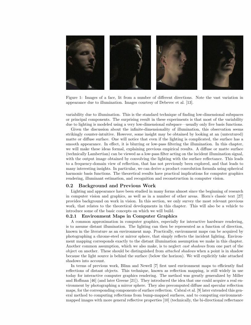
shading, specularities and shadows change. For instance, some images of a face under differentlighting conditions are shown in figure 1. Differences in lighting can often play a much greater rolein image variability of human faces than differences between individual people. Lighting designers inmovies can often set the mood of a scene with carefully chosen lighting. To achieve a sinister effect,for instance, one can use illumination from below the subject—a sharp contrast to most naturalindoor or outdoor scenes where the dominant light sources are above the person.

Characterizing the variability in appearance with lighting is a fundamental problem in many areasof computer vision, face modeling, and computer graphics. One of the great challenges of computervision is to produce systems that can work in uncontrolled environments. To be robust, recognitionsystems must be able to work oudoors in a lighting-insensitive manner. In computer graphics, thechallenge is to be able to efficiently create the visual appearance of a scene under realistic, possiblychanging, illumination.

At first glance, modeling the variation with lighting may seem intractable. For instance, a videoprojector can illuminate an object like a face with essentially any pattern. In this chapter, we willstay away from such extreme examples, making a set of assumptions that are approximately truein many common situations. One assumption we make is that illumination is distant. By this, wemean that the direction to, and intensity of, the light sources is approximately the same throughoutthe region of interest. This explicitly rules out cases like slide projectors. This is a reasonably goodapproximation in outdoor scenes, where the sky can be assumed to be far away. It is also fairlyaccurate in many indoor environments, where the light sources can be considered much further awayrelative to the size of the object.

Even under the assumption of distant lighting, the variations may seem intractable. The illumi-nation can come from any incident direction, and can be composed of multiple illuminants includinglocalized light sources like sunlight and broad area distributions like skylight. In the general case, wewould need to model the intensity from each of infinitely many incident lighting directions. Thus,the space we are dealing with appears to be infinite-dimensional. By contrast, a number of othercauses of appearance variation are low-dimensional. For instance, appearance varies with viewingdirection as well. However, unlike lighting, there can only be a single view direction. In general,variation because of pose and translation can be described using only six degrees of freedom.

Given the daunting nature of this problem, it is not surprising that most previous analytic mod-els have been restricted to the case of a single directional (distant) light source, usually withoutconsidering shadows. In computer graphics, this model is sufficient (but not necessarily efficient) fornumerical Monte Carlo simulation of appearance, since one can simply treat multiple light sourcesseparately and add up the results. In computer vision, such models can be reasonable approxima-tions under some circumstances, such as controlled laboratory conditions. However, they do notsuffice for modeling illumination variation in uncontrolled conditions like the outdoors.

Fortunately, there is an obvious empirical method of analyzing illumination variation. One cansimply record a number of images of an object under light sources from all different directions. Inpractice, this usually corresponds to moving a light source in a sphere around the object or person,while keeping camera and pose fixed. Because of the linearity of light transport—the image undermultiple lights is the sum of that under the individual sources—an image under arbitrary distantillumination can be written as a linear combination of these source images. This observation in itselfprovides an attractive direct approach for relighting in computer graphics. Furthermore, instead ofusing the source images, we can try to find linear combinations or basis images that best explain the

Figure 1: Images of a face, lit from a number of different directions. Note the vast variation inappearance due to illumination. Images courtesy of Debevec et al. [13].

variability due to illumination. This is the standard technique of finding low-dimensional subspacesor principal components. The surprising result in these experiments is that most of the variabilitydue to lighting is modeled using a very low-dimensional subspace—usually only five basis functions.

Given the discussion about the infinite-dimensionality of illumination, this observation seemsstrikingly counter-intuitive. However, some insight may be obtained by looking at an (untextured)matte or diffuse surface. One will notice that even if the lighting is complicated, the surface has asmooth appearance. In effect, it is blurring or low-pass filtering the illumination. In this chapter,we will make these ideas formal, explaining previous empirical results. A diffuse or matte surface(technically Lambertian) can be viewed as a low-pass filter acting on the incident illumination signal,with the output image obtained by convolving the lighting with the surface reflectance. This leadsto a frequency-domain view of reflection, that has not previously been explored, and that leads tomany interesting insights. In particular, we can derive a product convolution formula using sphericalharmonic basis functions. The theoretical results have practical implications for computer graphicsrendering, illuminant estimation, and recognition and reconstruction in computer vision.

0.2 Background and Previous WorkLighting and appearance have been studied in many forms almost since the beginning of research

in computer vision and graphics, as well as in a number of other areas. Horn’s classic text [27]provides background on work in vision. In this section, we only survey the most relevant previouswork, that relates to the theoretical developments in this chapter. This will also be a vehicle tointroduce some of the basic concepts on which we will build.

0.2.1 Environment Maps in Computer GraphicsA common approximation in computer graphics, especially for interactive hardware rendering,

is to assume distant illumination. The lighting can then be represented as a function of direction,known in the literature as an environment map. Practically, environment maps can be acquired byphotographing a chrome-steel or mirror sphere, that simply reflects the incident lighting. Environ-ment mapping corresponds exactly to the distant illumination assumption we make in this chapter.Another common assumption, which we also make, is to neglect cast shadows from one part of theobject on another. These should be distinguished from attached shadows when a point is in shadowbecause the light source is behind the surface (below the horizon). We will explicitly take attachedshadows into account.

In terms of previous work, Blinn and Newell [7] first used environment maps to efficiently findreflections of distant objects. This technique, known as reflection mapping, is still widely in usetoday for interactive computer graphics rendering. The method was greatly generalized by Millerand Hoffman [46] (and later Greene [21]). They introduced the idea that one could acquire a real en-vironment by photographing a mirror sphere. They also precomputed diffuse and specular reflectionmaps, for the corresponding components of surface reflection. Cabral et al. [9] later extended this gen-eral method to computing reflections from bump-mapped surfaces, and to computing environment-mapped images with more general reflective properties [10] (technically, the bi-directional reflectance

distribution function or BRDF [52]). Similar results for more general materials were also obtained byKautz et al. [32, 33], building on previous work by Heidrich and Seidel [25]. It should be noted thatboth Miller and Hoffman [46], and Cabral et al. [9, 10] qualitatively described the reflection mapsas obtained by convolving the lighting with the reflective properties of the surface. Kautz et al. [33]actually used convolution to implement reflection, but on somewhat distorted planar projections ofthe environment map, and without full theoretical justification. In this chapter, we will formalizethese ideas, making the notion of convolution precise, and derive analytic formulas.

0.2.2 Lighting-Insensitive Recognition in Computer VisionAnother important area of research is in computer vision, where there has been much work

on modeling the variation of appearance with lighting for robust lighting-insensitive recognitionalgorithms. Some of this prior work is discussed in detail in the excellent chapter on the effect ofillumination and face recognition by Ho and Kriegman in this volume. Illumination modeling is alsoimportant in many other vision problems, such as photometric stereo and structure from motion.

The work in this area has taken two directions. One approach is to apply an image processing op-erator that is relatively insensitive to the lighting. Work in this domain includes image gradients [8],the direction of the gradient [11], and Gabor jets [37]. While these methods reduce the effects oflighting variation, they operate without knowledge of the scene geometry, and so are inherentlylimited in the ability to model illumination variation. A number of empirical studies have suggestedthe difficulties of pure image-processing methods, in terms of achieving lighting-insensitivity [47].Our approach is more related to a second line of work that seeks to explicitly model illuminationvariation, analyzing the effects of the lighting on a 3D model of the object (here, a face).

Linear 3D Lighting Model Without Shadows: Within this category, a first important result(Shashua [69], Murase and Nayar [48], and others) is that for Lambertian objects, in the absenceof both attached and cast shadows, the images under all possible illumination conditions lie in athree-dimensional subspace. To obtain this result, let us first consider a model for the illuminationfrom a single directional source on a Lambertian object.

B = ρL(ω · n) = L · N , (1)

where L in the first relation corresponds to the intensity of the illumination in direction ω, n is thesurface normal at the point, ρ is the surface albedo and B is the outgoing radiosity (radiant exitance)or reflected light. For a nomenclature of radiometric quantities, see a textbook, like McCluney [45]or chapter 2 of Cohen and Wallance [12].1 It is sometimes useful to incorporate the albedo into thesurface normal, defining vectors N = ρn and correspondingly L = Lω, so we can simply write (forLambertian surfaces in the absence of all shadows, attached or cast) B = L · N .

Now, consider illumination from a variety of light sources L1,L2 and so on. It is straighforwardto use the linearity of light transport to write the net reflected light as

B =∑

i

Li · N =

(

∑

i

Li

)

· N = L · N , (2)

where L =∑

i Li. But this has essentially the same form as equation 1. Thus, in the absence ofall shadows, there is a very simple linear model for lighting in Lambertian surfaces, where we canreplace a complex lighting distribution by the weighted sum of the individual light sources. We canthen treat the object as if lit by a single effective light source L.

Finally, it is easy to see that images under all possible lighting conditions lie in a 3D subspace,being linear combinations of the cartesian components Nx, Ny, Nz, with B = LxNx + LyNy + LzNz.Note that this entire analysis applies to all points on the object. The basis images of the 3D lightingsubspace are simply the Cartesian components of the surface normals over the objects, scaled bythe albedos at those surface locations2.

1In general, we will use B for the reflected radiance, and L for the incident radiance, while ρ will denote the BRDF.For Lambertian surfaces, it is conventional to use ρ to denote the albedo (technically, the surface reflectance that liesbetween 0 and 1), which is π times the BRDF. Interpreting B as the radiosity accounts for this factor of π.

2Color is largely ignored in this chapter; we assume each color band, such as red, green and blue, is treatedseparately.

The 3D linear subspace has been used in a number of works on recognition, as well as otherareas. For instance, Hayakawa [24] used factorization based on the 3D subspace to build modelsusing photometric stereo. Koenderink and van Doorn [35] added an extra ambient term to makethis a 4D subspace. The extra term corresponds to perfectly diffuse lighting over the whole sphereof incoming directions. This corresponds to adding the albedos over the surface themselves to the

previous 3D subspace, i.e. adding ρ =‖ N ‖=√

N2x + N2

y + N2z .

Empirical Low-Dimensional Models: These theoretical results have inspired a number ofauthors to develop empirical models for lighting variability. As described in the introduction, onetakes a number of images with different lighting directions, and then uses standard dimensionalityreduction methods like Principal Component Analysis. PCA-based methods were pioneered for facesby Kirby and Sirovich [34, 72], and for face recognition by Turk and Pentland [78], but these authorsdid not account for variations due to illumination.

The effects of lighting alone were studied in a series of experiments by Hallinan [23], Epsteinet al. [15], and Yuille et al. [80]. They found that for human faces, and other diffuse objects likebasketballs, a 5D subspace sufficed to approximate lighting variability very well. That is, witha linear combination of a mean and 5 basis images, we can accurately predict appearance underarbitrary illumination. Furthermore, the form of these basis functions, and even the amount ofvariance accounted for, were largely consistent across human faces. For instance, Epstein et al. [15]report that for images of a human face, three basis images capture 90% of image variance, while fivebasis images account for 94%.

At the time however, these results had no complete theoretical explanation. Furthermore, theyindicate that the 3D subspace given above is inadequate. This is not difficult to understand. If weconsider the appearance of a face in outdoor lighting from the entire sky, there will often be attachedshadows or regions in the environment that are not visible to a given surface point (these correspondto lighting below the horizon for that point, where ω · n < 0).

Theoretical Models: The above discussion indicates the value of developing an analytic modelto account for lighting variability. Theoretical results can give new insights, and also lead to simplerand more efficient and robust algorithms.

Belhumeur and Kriegman [6] have taken a first step in this direction, developing the illumina-tion cone representation. Under very mild assumptions, the images of an object under arbitrarylighting form a convex cone in image space. In a sense, this follows directly from the linearity oflight transport. Any image can be scaled by a positive value simply by scaling the illumination.The convexity of the cone is because one can add two images, simply by adding the correspondinglighting. Formally, even for a Lambertian object with only attached shadows, the dimension of theillumination cone can be infinite (this grows as O(n2), where n is the number of distinct surfacenormals visible in the image). Georghiades et al. [19, 20] have developed recognition algorithmsbased on the illumination cone. One approach is to sample the cone using extremal rays, corre-sponding to rendering or imaging the face using directional light sources. It should be noted thatexact recognition using the illumination cone involves a slow complex optimization (constrainedoptimization must be used to enforce a non-negative linear combination of the basis images), andmethods using low-dimensional linear subspaces and unconstrained optimization (which essentiallyreduces to a simple linear system) are more efficient and usually required for practical applications.

Another approach is to try to analytically construct the principal component decomposition,analogous to what was done experimentally. Numerical PCA techniques could be biased by thespecific lighting conditions used, so an explicit analytic method is helpful. It is only recently thatthere has been progress in analytic methods for extending PCA from a discrete set of images to acontinuous sampling [40, 83]. These approaches demonstrate better generalization properties thanpure empirical techniques. In fact, Zhao and Yang [83] have analytically constructed the co-variancematrix for PCA of lighting variability, but under the assumption of no shadows.

Summary: To summarize, prior to the work reported in this chapter, the illumination variabilitycould be described theoretically by the illumination cone. It was known from numerical and realexperiments that the illumination cone lay close to a linear low-dimensional space for Lambertianobjects with attached shadows. However, a theoretical explanation of these results was not available.In this chapter, we develop a simple linear lighting model using spherical harmonics. These theoret-ical results were first introduced for Lambertian surfaces simultaneously by Basri and Jacobs [2, 4]and Ramamoorthi and Hanrahan [64]. Much of the work of Basri and Jacobs is also summarized inan excellent book chapter on illumination modeling for face recognition [5].

0.2.3 Frequency-Space Representations: Spherical Harmonics

We show reflection to be a convolution and analyze it in frequency space. We will primarily beconcerned with analyzing quantities like the BRDF and distant lighting, which can be parameterizedas functions on the unit sphere. Hence, the appropriate frequency-space representations are sphericalharmonics [28, 29, 42]. Spherical harmonics can be thought of as signal-processing tools on the unitsphere, analogous to the Fourier series or sines and cosines on the line or circle. They can bewritten either as trigonometric functions of the spherical coordinates, or as simple polynomials ofthe Cartesian components. They form an orthonormal basis on the unit sphere, in terms of whichquantities like the lighting or BRDF can be expanded and analyzed.

The use of spherical harmonics to represent the illumination and BRDF was pioneered in computergraphics by Cabral et al. [9]. In perception, D’Zmura [14] analyzed reflection as a linear operatorin terms of spherical harmonics, and discussed some resulting ambiguities between reflectance andillumination. Our use of spherical harmonics to represent the lighting is also similar in some respectsto previous methods such as that of Nimeroff et al. [56] that use steerable linear basis functions.Spherical harmonics have also been used before in computer graphics for representing BRDFs by anumber of other authors [70, 79].

The results described in this chapter are based on a number of papers by us. This includestheoretical work in the planar 2D case or flatland [62], on the analysis of the appearance of aLambertian surface using spherical harmonics [64], the theory for the general 3D case with isotropicBRDFs [65], and a comprehensive account including a unified view of 2D and 3D cases includinganisotropic materials [67]. More details can also be found in the PhD thesis of the author [61].Recently, we have also linked the convolution approach using spherical harmonics with principalcomponent analysis, quantitatively explaining previous empirical results on lighting variability [60].

0.3 Analyzing Lambertian Reflection using Spherical Harmonics

In this section, we analyze the important case of Lambertian surfaces under distant illumina-tion [64], using spherical harmonics. We will derive a simple linear relationship, where the coeffi-cients of the reflected light are simply filtered versions of the incident illumination. Furthermore, alow frequency approximation with only 9 spherical harmonic terms is shown to be accurate.

Assumptions: Mathematically, we are simply considering the relationship between the irradiance(a measure of the intensity of incident light, reflected equally in all directions by diffuse objects),expressed as a function of surface orientation, and the incoming radiance or incident illumination,expressed as a function of incident angle. The corresponding physical system is a curved convexhomogeneous Lambertian surface reflecting a distant illumination field. For the physical system, wewill assume that the surfaces under consideration are convex, so they may be parameterized by thesurface orientation, as described by the surface normal, and so that interreflection and cast shadowing(but not attached shadows) can be ignored. Also, surfaces will be assumed to be Lambertian andhomogeneous, so the reflectivity can be characterized by a constant albedo. We will further assumehere that the illuminating light sources are distant, so the illumination or incoming radiance can berepresented as a function of direction only.

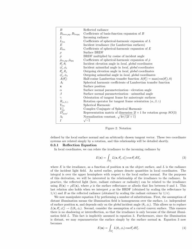
Notation used in the chapter (some of which pertains to later sections) is listed in table 2. Adiagram of the local geometry of the situation is shown in figure 3. We will use two types ofcoordinates. Unprimed global coordinates denote angles with respect to a global reference frame.On the other hand, primed local coordinates denote angles with respect to the local reference frame,

B Reflected radianceBlmn,pq, Blmpq Coefficients of basis-function expansion of BL Incoming radianceLlm Coefficients of spherical-harmonic expansion of LE Incident irradiance (for Lambertian surfaces)Elm Coefficients of spherical-harmonic expansion of Eρ Surface BRDFρ BRDF multiplied by cosine of incident angleρln,pq, ρlpq Coefficients of spherical-harmonic expansion of ρθ′i, θi Incident elevation angle in local, global coordinatesφ′

i, φi Incident azimuthal angle in local, global coordinatesθ′o, θo Outgoing elevation angle in local, global coordinatesφ′

o, φo Outgoing azimuthal angle in local, global coordinatesA(θ′i) Half-cosine Lambertian transfer function A(θ′i) = max(cos(θ′i), 0)Al Spherical harmonic coefficients of Lambertian transfer functionx Surface positionα Surface normal parameterization—elevation angleβ Surface normal parameterization—azimuthal angleγ Orientation of tangent frame for anisotropic surfacesRα,β,γ Rotation operator for tangent frame orientation (α, β, γ)Ylm Spherical HarmonicY ∗

lm Complex Conjugate of Spherical HarmonicDl

mm′ Representation matrix of dimension 2l + 1 for rotation group SO(3)

Λl Normalization constant,√

4π/(2l + 1)I

√−1

Figure 2: Notation

defined by the local surface normal and an arbitrarily chosen tangent vector. These two coordinatesystems are related simply by a rotation, and this relationship will be detailed shortly.

0.3.1 Reflection EquationIn local coordinates, we can relate the irradiance to the incoming radiance by

E(x) =

∫

Ω′

i

L(x, θ′i, φ′

i) cos θ′i dΩ′

i, (3)

where E is the irradiance, as a function of position x on the object surface, and L is the radianceof the incident light field. As noted earlier, primes denote quantities in local coordinates. Theintegral is over the upper hemisphere with respect to the local surface normal. For the purposesof this derivation, we will be interested in the relationship of the irradiance to the radiance. Inpractice, the reflected light (here, radiant exitance or radiosity) can be related to the irradianceusing B(x) = ρE(x), where ρ is the surface reflectance or albedo that lies between 0 and 1. Thislast relation also holds when we interpret ρ as the BRDF (obtained by scaling the reflectance by1/π) and B as the reflected radiance (obtained by scaling the radiant exitance by 1/π).

We now manipulate equation 3 by performing a number of substitutions. First, the assumption ofdistant illumination means the illumination field is homogeneous over the surface, i.e. independentof surface position x, and depends only on the global incident angle (θi, φi). This allows us to replaceL(x, θ′i, φ

′

i) → L(θi, φi). Second, consider the assumption of a curved convex surface. This ensuresthere is no shadowing or interreflection, so that the irradiance is only because of the distant illumi-nation field L. This fact is implicitly assumed in equation 3. Furthermore, since the illuminationis distant, we may reparameterize the surface simply by the surface normal n. Equation 3 nowbecomes

E(n) =

∫

Ω′

i

L(θi, φi) cos θ′i dΩ′

i. (4)

Y’

o

o’θ

’Z

θ

’ Xφi ’

’φ

’i

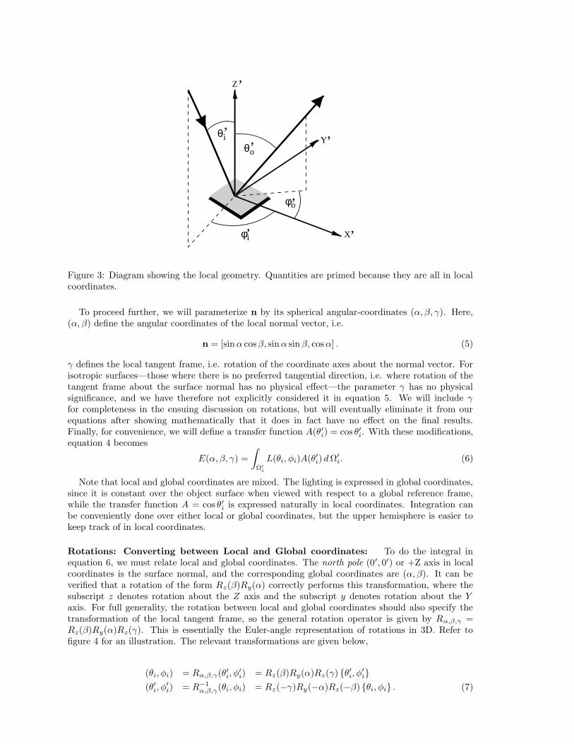
Figure 3: Diagram showing the local geometry. Quantities are primed because they are all in localcoordinates.

To proceed further, we will parameterize n by its spherical angular-coordinates (α, β, γ). Here,(α, β) define the angular coordinates of the local normal vector, i.e.

n = [sin α cosβ, sin α sin β, cos α] . (5)

γ defines the local tangent frame, i.e. rotation of the coordinate axes about the normal vector. Forisotropic surfaces—those where there is no preferred tangential direction, i.e. where rotation of thetangent frame about the surface normal has no physical effect—the parameter γ has no physicalsignificance, and we have therefore not explicitly considered it in equation 5. We will include γfor completeness in the ensuing discussion on rotations, but will eventually eliminate it from ourequations after showing mathematically that it does in fact have no effect on the final results.Finally, for convenience, we will define a transfer function A(θ′

i) = cos θ′i. With these modifications,equation 4 becomes

E(α, β, γ) =

∫

Ω′

i

L(θi, φi)A(θ′i) dΩ′

i. (6)

Note that local and global coordinates are mixed. The lighting is expressed in global coordinates,since it is constant over the object surface when viewed with respect to a global reference frame,while the transfer function A = cos θ′i is expressed naturally in local coordinates. Integration canbe conveniently done over either local or global coordinates, but the upper hemisphere is easier tokeep track of in local coordinates.

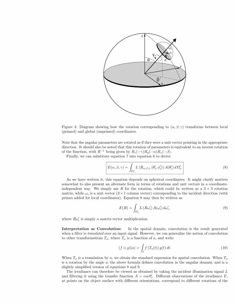
Rotations: Converting between Local and Global coordinates: To do the integral inequation 6, we must relate local and global coordinates. The north pole (0′, 0′) or +Z axis in localcoordinates is the surface normal, and the corresponding global coordinates are (α, β). It can beverified that a rotation of the form Rz(β)Ry(α) correctly performs this transformation, where thesubscript z denotes rotation about the Z axis and the subscript y denotes rotation about the Yaxis. For full generality, the rotation between local and global coordinates should also specify thetransformation of the local tangent frame, so the general rotation operator is given by Rα,β,γ =Rz(β)Ry(α)Rz(γ). This is essentially the Euler-angle representation of rotations in 3D. Refer tofigure 4 for an illustration. The relevant transformations are given below,

(θi, φi) = Rα,β,γ(θ′i, φ′

i) = Rz(β)Ry(α)Rz(γ) θ′i, φ′

i(θ′i, φ

′

i) = R−1α,β,γ(θi, φi) = Rz(−γ)Ry(−α)Rz(−β) θi, φi . (7)

Z

αY’

β

Z’

γ

X’

X

Y

Figure 4: Diagram showing how the rotation corresponding to (α, β, γ) transforms between local(primed) and global (unprimed) coordinates.

Note that the angular parameters are rotated as if they were a unit vector pointing in the appropriatedirection. It should also be noted that this rotation of parameters is equivalent to an inverse rotationof the function, with R−1 being given by Rz(−γ)Ry(−α)Rz(−β).

Finally, we can substitute equation 7 into equation 6 to derive

E(α, β, γ) =

∫

Ω′

i

L (Rα,β,γ (θ′i, φ′

i)) A(θ′i) dΩ′

i. (8)

As we have written it, this equation depends on spherical coordinates. It might clarify matterssomewhat to also present an alternate form in terms of rotations and unit vectors in a coordinate-independent way. We simply use R for the rotation, which could be written as a 3 × 3 rotationmatrix, while ωi is a unit vector (3× 1 column vector) corresponding to the incident direction (withprimes added for local coordinates). Equation 8 may then be written as

E(R) =

∫

Ω′

i

L (Rω′

i) A(ω′

i) dω′

i, (9)

where Rω′

i is simply a matrix-vector multiplication.

Interpretation as Convolution: In the spatial domain, convolution is the result generatedwhen a filter is translated over an input signal. However, we can generalize the notion of convolutionto other transformations Ta, where Ta is a function of a, and write

(f ⊗ g)(a) =

∫

t

f (Ta(t)) g(t) dt. (10)

When Ta is a translation by a, we obtain the standard expression for spatial convolution. When Ta

is a rotation by the angle a, the above formula defines convolution in the angular domain, and is aslightly simplified version of equations 8 and 9.

The irradiance can therefore be viewed as obtained by taking the incident illumination signal Land filtering it using the transfer function A = cos θ′i. Different observations of the irradiance E,at points on the object surface with different orientations, correspond to different rotations of the

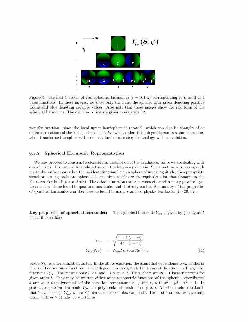
Figure 5: The first 3 orders of real spherical harmonics (l = 0, 1, 2) corresponding to a total of 9basis functions. In these images, we show only the front the sphere, with green denoting positivevalues and blue denoting negative values. Also note that these images show the real form of thespherical harmonics. The complex forms are given in equation 12.

transfer function—since the local upper hemisphere is rotated—which can also be thought of asdifferent rotations of the incident light field. We will see that this integral becomes a simple productwhen transformed to spherical harmonics, further stressing the analogy with convolution.

0.3.2 Spherical Harmonic Representation

We now proceed to construct a closed-form description of the irradiance. Since we are dealing withconvolutions, it is natural to analyze them in the frequency domain. Since unit vectors correspond-ing to the surface normal or the incident direction lie on a sphere of unit magnitude, the appropriatesignal-processing tools are spherical harmonics, which are the equivalent for that domain to theFourier series in 2D (on a circle). These basis functions arise in connection with many physical sys-tems such as those found in quantum mechanics and electrodynamics. A summary of the propertiesof spherical harmonics can therefore be found in many standard physics textbooks [28, 29, 42].

Key properties of spherical harmonics: The spherical harmonic Ylm is given by (see figure 5for an illustration)

Nlm =

√

2l + 1

4π

(l − m)!

(l + m)!

Ylm(θ, φ) = NlmPlm(cos θ)eImφ, (11)

where Nlm is a normalization factor. In the above equation, the azimuthal dependence is expanded interms of Fourier basis functions. The θ dependence is expanded in terms of the associated Legendrefunctions Plm. The indices obey l ≥ 0 and −l ≤ m ≤ l. Thus, there are 2l + 1 basis functions forgiven order l. They may be written either as trigonometric functions of the spherical coordinatesθ and φ or as polynomials of the cartesian components x, y and z, with x2 + y2 + z2 = 1. Ingeneral, a spherical harmonic Ylm is a polynomial of maximum degree l. Another useful relation isthat Yl−m = (−1)mY ∗

lm, where Y ∗

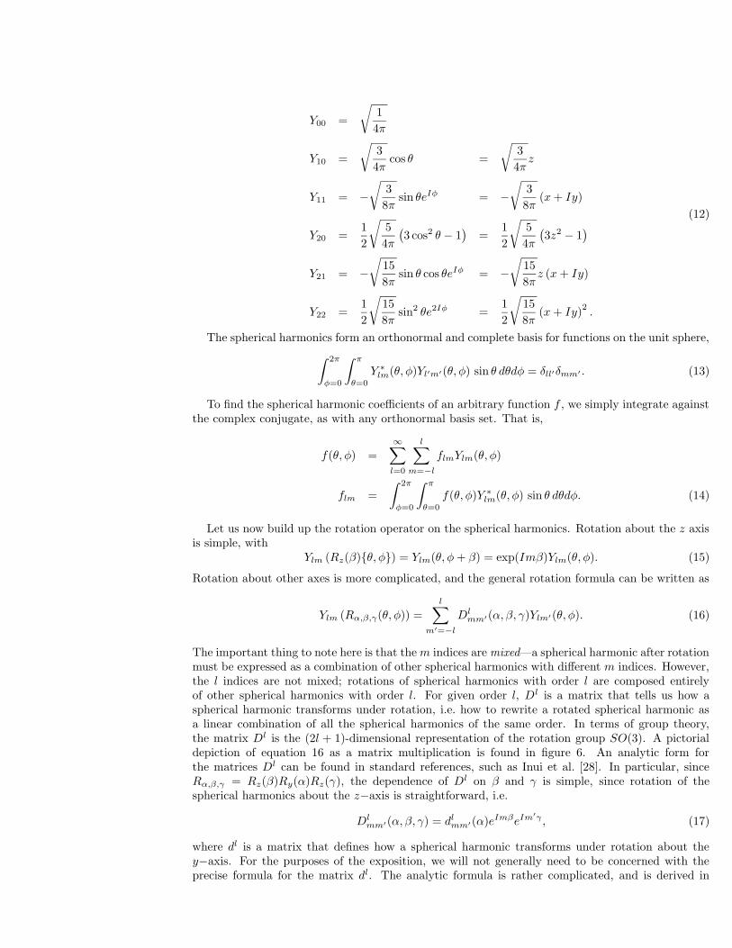
lm denotes the complex conjugate. The first 3 orders (we give onlyterms with m ≥ 0) may be written as

Y00 =

√

1

4π

Y10 =

√

3

4πcos θ =

√

3

4πz

Y11 = −√

3

8πsin θeIφ = −

√

3

8π(x + Iy)

Y20 =1

2

√

5

4π

(

3 cos2 θ − 1)

=1

2

√

5

4π

(

3z2 − 1)

Y21 = −√

15

8πsin θ cos θeIφ = −

√

15

8πz (x + Iy)

Y22 =1

2

√

15

8πsin2 θe2Iφ =

1

2

√

15

8π(x + Iy)

2.

(12)

The spherical harmonics form an orthonormal and complete basis for functions on the unit sphere,

∫ 2π

φ=0

∫ π

θ=0

Y ∗

lm(θ, φ)Yl′m′(θ, φ) sin θ dθdφ = δll′δmm′ . (13)

To find the spherical harmonic coefficients of an arbitrary function f , we simply integrate againstthe complex conjugate, as with any orthonormal basis set. That is,

f(θ, φ) =∞∑

l=0

l∑

m=−l

flmYlm(θ, φ)

flm =

∫ 2π

φ=0

∫ π

θ=0

f(θ, φ)Y ∗

lm(θ, φ) sin θ dθdφ. (14)

Let us now build up the rotation operator on the spherical harmonics. Rotation about the z axisis simple, with

Ylm (Rz(β)θ, φ) = Ylm(θ, φ + β) = exp(Imβ)Ylm(θ, φ). (15)

Rotation about other axes is more complicated, and the general rotation formula can be written as

Ylm (Rα,β,γ(θ, φ)) =

l∑

m′=−l

Dlmm′(α, β, γ)Ylm′(θ, φ). (16)

The important thing to note here is that the m indices are mixed—a spherical harmonic after rotationmust be expressed as a combination of other spherical harmonics with different m indices. However,the l indices are not mixed; rotations of spherical harmonics with order l are composed entirelyof other spherical harmonics with order l. For given order l, Dl is a matrix that tells us how aspherical harmonic transforms under rotation, i.e. how to rewrite a rotated spherical harmonic asa linear combination of all the spherical harmonics of the same order. In terms of group theory,the matrix Dl is the (2l + 1)-dimensional representation of the rotation group SO(3). A pictorialdepiction of equation 16 as a matrix multiplication is found in figure 6. An analytic form forthe matrices Dl can be found in standard references, such as Inui et al. [28]. In particular, sinceRα,β,γ = Rz(β)Ry(α)Rz(γ), the dependence of Dl on β and γ is simple, since rotation of thespherical harmonics about the z−axis is straightforward, i.e.

Dlmm′(α, β, γ) = dl

mm′(α)eImβeIm′γ , (17)

where dl is a matrix that defines how a spherical harmonic transforms under rotation about they−axis. For the purposes of the exposition, we will not generally need to be concerned with theprecise formula for the matrix dl. The analytic formula is rather complicated, and is derived in

Y00

Y1−1

Y10

Y11

Y2−2

Y2−1

Y20

Y21

Y22

. . .

=

D000

D1−1−1 D1

−10 D1−11

D10−1 D1

00 D101

D11−1 D1

10 D111

D2−2−2 D2

−2−1 D2−20 D2

−21 D2−22

D2−1−2 D2

−1−1 D2−10 D2

−11 D2−12

D20−2 D2

0−1 D200 D2

01 D202

D21−2 D2

1−1 D210 D2

11 D212

D22−2 D2

2−1 D220 D2

21 D222

. . .

Y00

Y1−1

Y10

Y11

Y2−2

Y2−1

Y20

Y21

Y22

. . .

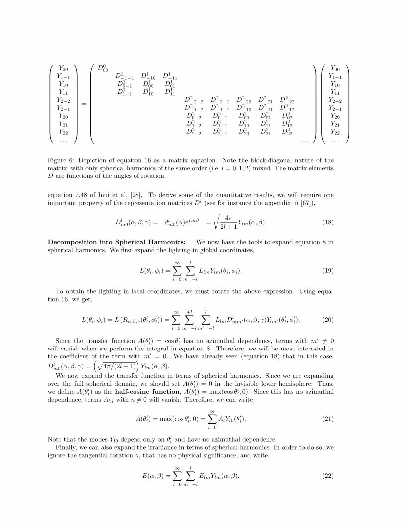
Figure 6: Depiction of equation 16 as a matrix equation. Note the block-diagonal nature of thematrix, with only spherical harmonics of the same order (i.e. l = 0, 1, 2) mixed. The matrix elementsD are functions of the angles of rotation.

equation 7.48 of Inui et al. [28], To derive some of the quantitative results, we will require oneimportant property of the representation matrices Dl (see for instance the appendix in [67]),

Dlm0(α, β, γ) = dl

m0(α)eImβ =

√

4π

2l + 1Ylm(α, β). (18)

Decomposition into Spherical Harmonics: We now have the tools to expand equation 8 inspherical harmonics. We first expand the lighting in global coordinates,

L(θi, φi) =∞∑

l=0

l∑

m=−l

LlmYlm(θi, φi). (19)

To obtain the lighting in local coordinates, we must rotate the above expression. Using equa-tion 16, we get,

L(θi, φi) = L (Rα,β,γ(θ′i, φ′

i)) =

∞∑

l=0

+l∑

m=−l

l∑

m′=−l

LlmDlmm′(α, β, γ)Ylm′(θ′i, φ

′

i). (20)

Since the transfer function A(θ′i) = cos θ′i has no azimuthal dependence, terms with m′ 6= 0will vanish when we perform the integral in equation 8. Therefore, we will be most interested inthe coefficient of the term with m′ = 0. We have already seen (equation 18) that in this case,

Dlm0(α, β, γ) =

(

√

4π/(2l + 1))

Ylm(α, β).

We now expand the transfer function in terms of spherical harmonics. Since we are expandingover the full spherical domain, we should set A(θ′i) = 0 in the invisible lower hemisphere. Thus,we define A(θ′i) as the half-cosine function, A(θ′i) = max(cos θ′i, 0). Since this has no azimuthaldependence, terms Aln with n 6= 0 will vanish. Therefore, we can write

A(θ′i) = max(cos θ′i, 0) =∞∑

l=0

AlYl0(θ′

i). (21)

Note that the modes Yl0 depend only on θ′i and have no azimuthal dependence.Finally, we can also expand the irradiance in terms of spherical harmonics. In order to do so, we

ignore the tangential rotation γ, that has no physical significance, and write

E(α, β) =

∞∑

l=0

l∑

m=−l

ElmYlm(α, β). (22)

0 2 4 6 8 10 12 14 16 18 20−0.2

0

0.2

0.4

0.6

0.8

1

1.2

l −>La

mbe

rtia

n br

df c

oeffi

cien

t −>

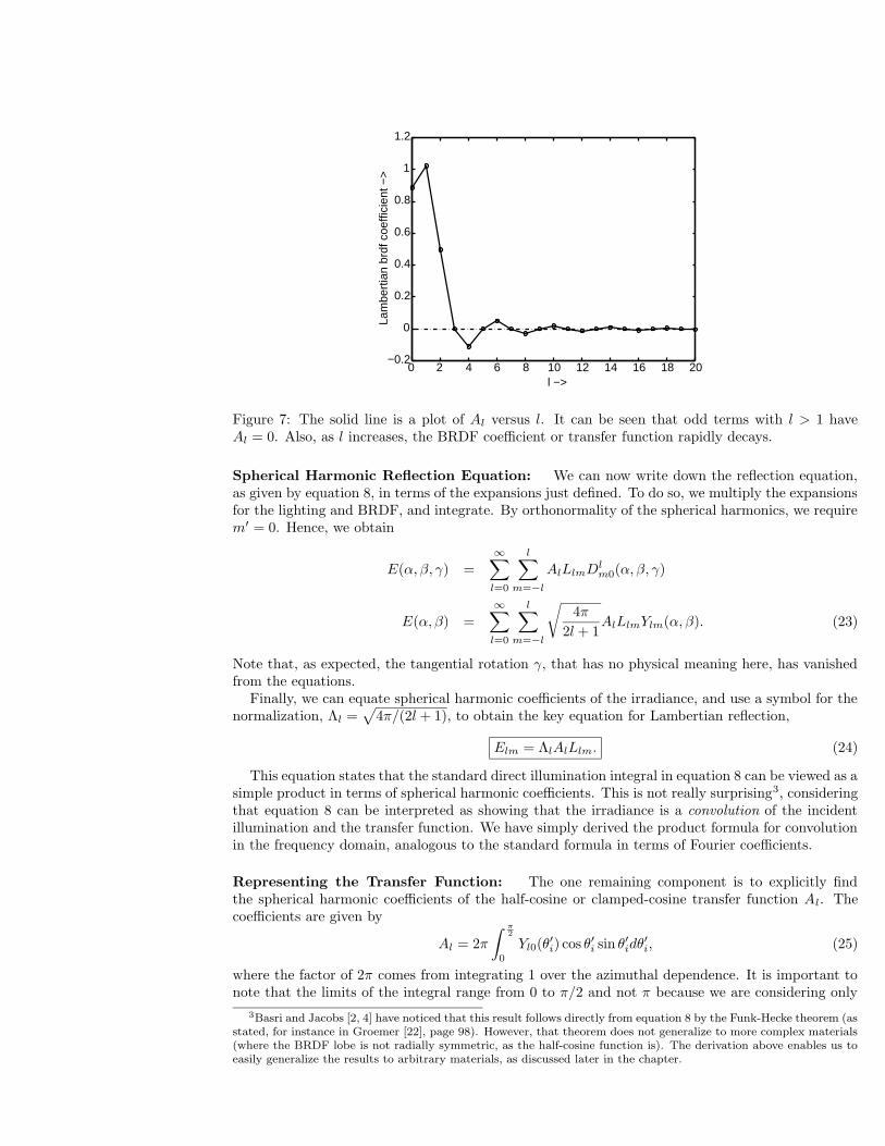
Figure 7: The solid line is a plot of Al versus l. It can be seen that odd terms with l > 1 haveAl = 0. Also, as l increases, the BRDF coefficient or transfer function rapidly decays.

Spherical Harmonic Reflection Equation: We can now write down the reflection equation,as given by equation 8, in terms of the expansions just defined. To do so, we multiply the expansionsfor the lighting and BRDF, and integrate. By orthonormality of the spherical harmonics, we requirem′ = 0. Hence, we obtain

E(α, β, γ) =

∞∑

l=0

l∑

m=−l

AlLlmDlm0(α, β, γ)

E(α, β) =∞∑

l=0

l∑

m=−l

√

4π

2l + 1AlLlmYlm(α, β). (23)

Note that, as expected, the tangential rotation γ, that has no physical meaning here, has vanishedfrom the equations.

Finally, we can equate spherical harmonic coefficients of the irradiance, and use a symbol for thenormalization, Λl =

√

4π/(2l + 1), to obtain the key equation for Lambertian reflection,

Elm = ΛlAlLlm. (24)

This equation states that the standard direct illumination integral in equation 8 can be viewed as asimple product in terms of spherical harmonic coefficients. This is not really surprising3, consideringthat equation 8 can be interpreted as showing that the irradiance is a convolution of the incidentillumination and the transfer function. We have simply derived the product formula for convolutionin the frequency domain, analogous to the standard formula in terms of Fourier coefficients.

Representing the Transfer Function: The one remaining component is to explicitly findthe spherical harmonic coefficients of the half-cosine or clamped-cosine transfer function Al. Thecoefficients are given by

Al = 2π

∫ π

2

0

Yl0(θ′

i) cos θ′i sin θ′idθ′i, (25)

where the factor of 2π comes from integrating 1 over the azimuthal dependence. It is important tonote that the limits of the integral range from 0 to π/2 and not π because we are considering only

3Basri and Jacobs [2, 4] have noticed that this result follows directly from equation 8 by the Funk-Hecke theorem (asstated, for instance in Groemer [22], page 98). However, that theorem does not generalize to more complex materials(where the BRDF lobe is not radially symmetric, as the half-cosine function is). The derivation above enables us toeasily generalize the results to arbitrary materials, as discussed later in the chapter.

0 0.5 1 1.5 2 2.5 3−0.4

−0.2

0

0.2

0.4

0.6

0.8

1Clamped Cosl=0 l=1 l=2 l=4

π/2 π

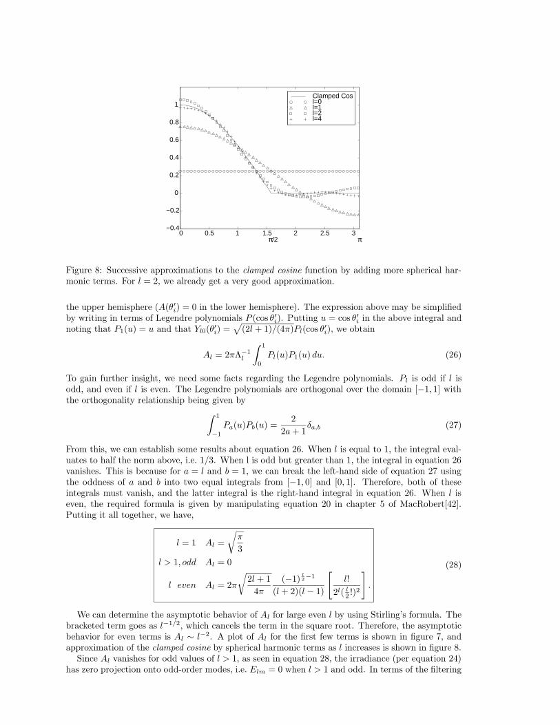
Figure 8: Successive approximations to the clamped cosine function by adding more spherical har-monic terms. For l = 2, we already get a very good approximation.

the upper hemisphere (A(θ′i) = 0 in the lower hemisphere). The expression above may be simplifiedby writing in terms of Legendre polynomials P (cos θ′i). Putting u = cos θ′i in the above integral andnoting that P1(u) = u and that Yl0(θ

′

i) =√

(2l + 1)/(4π)Pl(cos θ′i), we obtain

Al = 2πΛ−1l

∫ 1

0

Pl(u)P1(u) du. (26)

To gain further insight, we need some facts regarding the Legendre polynomials. Pl is odd if l isodd, and even if l is even. The Legendre polynomials are orthogonal over the domain [−1, 1] withthe orthogonality relationship being given by

∫ 1

−1

Pa(u)Pb(u) =2

2a + 1δa,b (27)

From this, we can establish some results about equation 26. When l is equal to 1, the integral eval-uates to half the norm above, i.e. 1/3. When l is odd but greater than 1, the integral in equation 26vanishes. This is because for a = l and b = 1, we can break the left-hand side of equation 27 usingthe oddness of a and b into two equal integrals from [−1, 0] and [0, 1]. Therefore, both of theseintegrals must vanish, and the latter integral is the right-hand integral in equation 26. When l iseven, the required formula is given by manipulating equation 20 in chapter 5 of MacRobert[42].Putting it all together, we have,

l = 1 Al =

√

π

3

l > 1, odd Al = 0

l even Al = 2π

√

2l + 1

4π

(−1)l

2−1

(l + 2)(l − 1)

[

l!

2l( l2 !)2

]

.

(28)

We can determine the asymptotic behavior of Al for large even l by using Stirling’s formula. Thebracketed term goes as l−1/2, which cancels the term in the square root. Therefore, the asymptoticbehavior for even terms is Al ∼ l−2. A plot of Al for the first few terms is shown in figure 7, andapproximation of the clamped cosine by spherical harmonic terms as l increases is shown in figure 8.

Since Al vanishes for odd values of l > 1, as seen in equation 28, the irradiance (per equation 24)has zero projection onto odd-order modes, i.e. Elm = 0 when l > 1 and odd. In terms of the filtering

analogy in signal-processing, since the filter corresponding to A(θ′

i) = cos θ′i destroys high-frequencyodd terms in the spherical harmonic expansion of the lighting, the corresponding terms are not foundin the irradiance. Further, for large even l, the asymptotic behavior of Elm ∼ l−5/2 since Al ∼ l−2.The transfer function A acts as a low pass filter, causing the rapid decay of high-frequency terms inthe lighting.

It is instructive to explicitly write out numerically the first few terms for the irradiance perequations 24 and 28,

E00 = πL00 ≈ 3.142L00

E1m = 2π3 L1m ≈ 2.094L1m

E2m = π4 L2m ≈ 0.785L2m

E3m = 0

E4m = − π24L4m ≈ −0.131L4m

E5m = 0

E6m = π64L6m ≈ 0.049L6m. (29)

We see that already for E4m, the coefficient is only about 1% of what it is for E00. Therefore,in real applications, where surfaces are only approximately Lambertian, and there are errors inmeasurement, we can obtain good results using an order 2 approximation of the illumination andirradiance. Since there are 2l + 1 indices (values of m, which ranges from −l to +l) for order l,this corresponds to 9 coefficients for l ≤ 2—1 term with order 0, 3 terms with order 1, and 5 termswith order 2. Note that the single order 0 mode Y00 is a constant, the 3 order 1 modes are linearfunctions of the Cartesian coordinates—in real form, they are simply x, y, and z—while the 5 order2 modes are quadratic functions of the Cartesian coordinates.

Therefore, the irradiance—or equivalently, the reflected light field from a convexLambertian object—can be well approximated using spherical harmonics up to order 2(a 9 term representation), i.e. as a quadratic polynomial of the Cartesian coordinatesof the surface normal vector. This is one of the key results of this chapter. By a careful formalanalysis, Basri and Jacobs [2, 4] have shown that over 99.2% of the energy of the filter is captured inorders 0,1 and 2, and 87.5% is captured even in an order 1 four term approximation. Furthermore,by enforcing non-negativity of the illumination, one can show that for any lighting conditions, theaverage accuracy of an order 2 approximation is at least 98%.

0.3.3 Explanation of Experimental ResultsHaving obtained the theoretical result connecting irradiance and radiance, we can now address

the empirical results on low dimensionality we discussed in the background section. First, considerimages under all possible illuminations. Since any image can be well described by a linear combina-tion of 9 terms—the images corresponding to the 9 lowest frequency spherical harmonic lights—weexpect the illumination variation to lie close to a 9-dimensional subspace. In fact, a 4D subspaceconsisting of the linear and constant terms itself accounts for almost 90% of the energy. This 4D sub-space is exactly that of Koenderink and van Doorn [35]. Similarly, the 3D subspace of Shashua [69]can be thought of as corresponding to the lighting from order 1 spherical harmonics only. However,this neglects the ambient or order 0 term, which is quite important from our analytic results.

There remain at this point two interesting theoretical questions. First, how does the sphericalharmonic convolution result connect to principal component analysis? Second, the 9D subspacepredicted by the above analysis does not completely agree with the 5D subspace observed in anumber of experiments [15, 23]. Recently, we have shown [60] that under appropriate assumptions,the principal components or eigenvectors are equal to the spherical harmonic basis functions and theeigenvalues, corresponding to how important a principal component is in explaining image variability,are equal to the spherical harmonic coefficients ΛlAl. Furthermore, if we see only a single image, asin previous experimental tests, only the front-facing normals, and not the entire sphere of surfacenormals is visible. This allows approximation by a lower-dimensional subspace. We have shown howto analyze this effect with spherical harmonics, deriving analytic forms for the principal componentsof canonical shapes. The results for a human face are shown in figure 9, and are in qualitative andquantitative agreement with previous empirical work, providing the first full theoretical explanation.

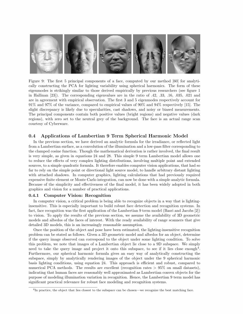
Figure 9: The first 5 principal components of a face, computed by our method [60] for analyti-cally constructing the PCA for lighting variability using spherical harmonics. The form of theseeigenmodes is strikingly similar to those derived empirically by previous researchers (see figure 1in Hallinan [23]). The corresponding eigenvalues are in the ratio of .42, .33, .16, .035, .021 andare in agreement with empirical observation. The first 3 and 5 eigenmodes respectively account for91% and 97% of the variance, compared to empirical values of 90% and 94% respectively [15]. Theslight discrepancy is likely due to specularities, cast shadows, and noisy or biased measurements.The principal components contain both positive values (bright regions) and negative values (darkregions), with zero set to the neutral grey of the background. The face is an actual range scancourtesy of Cyberware.

0.4 Applications of Lambertian 9 Term Spherical Harmonic Model

In the previous section, we have derived an analytic formula for the irradiance, or reflected lightfrom a Lambertian surface, as a convolution of the illumination and a low-pass filter corresponding tothe clamped cosine function. Though the mathematical derivation is rather involved, the final resultis very simple, as given in equations 24 and 28. This simple 9 term Lambertian model allows oneto reduce the effects of very complex lighting distributions, involving multiple point and extendedsources, to a simple quadratic formula. It therefore enables computer vision applications, that had sofar to rely on the simple point or directional light source model, to handle arbitrary distant lightingwith attached shadows. In computer graphics, lighting calculations that had previously requiredexpensive finite element or Monte Carlo integration, can now be done with a simple analytic formula.Because of the simplicity and effectiveness of the final model, it has been widely adopted in bothgraphics and vision for a number of practical applications.

0.4.1 Computer Vision: Recognition

In computer vision, a critical problem is being able to recognize objects in a way that is lighting-insensitive. This is especially important to build robust face detection and recognition systems. Infact, face recognition was the first application of the Lambertian 9 term model (Basri and Jacobs [2])to vision. To apply the results of the previous section, we assume the availability of 3D geometricmodels and albedos of the faces of interest. With the ready availability of range scanners that givedetailed 3D models, this is an increasingly reasonable assumption.

Once the position of the object and pose have been estimated, the lighting-insensitive recognitionproblem can be stated as follows. Given a 3D geometric model and albedos for an object, determineif the query image observed can correspond to the object under some lighting condition. To solvethis problem, we note that images of a Lambertian object lie close to a 9D subspace. We simplyneed to take the query image and project it onto this subspace, to see if it lies close enough4.Furthermore, our spherical harmonic formula gives an easy way of analytically constructing thesubspace, simply by analytically rendering images of the object under the 9 spherical harmonicbasis lighting conditions, using equation 24. This approach is efficient and robust, compared tonumerical PCA methods. The results are excellent (recognition rates > 95% on small datasets),indicating that human faces are reasonably well approximated as Lambertian convex objects for thepurpose of modeling illumination variation in recognition. Hence, the Lambertian 9 term model hassignificant practical relevance for robust face modeling and recognition systems.

4In practice, the object that lies closest to the subspace can be chosen—we recognize the best matching face.

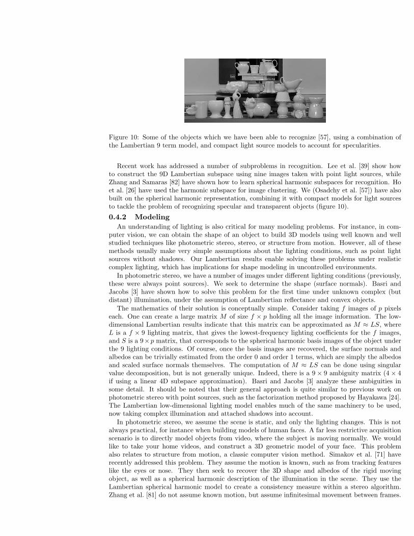
Figure 10: Some of the objects which we have been able to recognize [57], using a combination ofthe Lambertian 9 term model, and compact light source models to account for specularities.

Recent work has addressed a number of subproblems in recognition. Lee et al. [39] show howto construct the 9D Lambertian subspace using nine images taken with point light sources, whileZhang and Samaras [82] have shown how to learn spherical harmonic subspaces for recognition. Hoet al. [26] have used the harmonic subspace for image clustering. We (Osadchy et al. [57]) have alsobuilt on the spherical harmonic representation, combining it with compact models for light sourcesto tackle the problem of recognizing specular and transparent objects (figure 10).

0.4.2 Modeling

An understanding of lighting is also critical for many modeling problems. For instance, in com-puter vision, we can obtain the shape of an object to build 3D models using well known and wellstudied techniques like photometric stereo, stereo, or structure from motion. However, all of thesemethods usually make very simple assumptions about the lighting conditions, such as point lightsources without shadows. Our Lambertian results enable solving these problems under realisticcomplex lighting, which has implications for shape modeling in uncontrolled environments.

In photometric stereo, we have a number of images under different lighting conditions (previously,these were always point sources). We seek to determine the shape (surface normals). Basri andJacobs [3] have shown how to solve this problem for the first time under unknown complex (butdistant) illumination, under the assumption of Lambertian reflectance and convex objects.

The mathematics of their solution is conceptually simple. Consider taking f images of p pixelseach. One can create a large matrix M of size f × p holding all the image information. The low-dimensional Lambertian results indicate that this matrix can be approximated as M ≈ LS, whereL is a f × 9 lighting matrix, that gives the lowest-frequency lighting coefficients for the f images,and S is a 9×p matrix, that corresponds to the spherical harmonic basis images of the object underthe 9 lighting conditions. Of course, once the basis images are recovered, the surface normals andalbedos can be trivially estimated from the order 0 and order 1 terms, which are simply the albedosand scaled surface normals themselves. The computation of M ≈ LS can be done using singularvalue decomposition, but is not generally unique. Indeed, there is a 9 × 9 ambiguity matrix (4 × 4if using a linear 4D subspace approximation). Basri and Jacobs [3] analyze these ambiguities insome detail. It should be noted that their general approach is quite similar to previous work onphotometric stereo with point sources, such as the factorization method proposed by Hayakawa [24].The Lambertian low-dimensional lighting model enables much of the same machinery to be used,now taking complex illumination and attached shadows into account.

In photometric stereo, we assume the scene is static, and only the lighting changes. This is notalways practical, for instance when building models of human faces. A far less restrictive acquisitionscenario is to directly model objects from video, where the subject is moving normally. We wouldlike to take your home videos, and construct a 3D geometric model of your face. This problemalso relates to structure from motion, a classic computer vision method. Simakov et al. [71] haverecently addressed this problem. They assume the motion is known, such as from tracking featureslike the eyes or nose. They then seek to recover the 3D shape and albedos of the rigid movingobject, as well as a spherical harmonic description of the illumination in the scene. They use theLambertian spherical harmonic model to create a consistency measure within a stereo algorithm.Zhang et al. [81] do not assume known motion, but assume infinitesimal movement between frames.

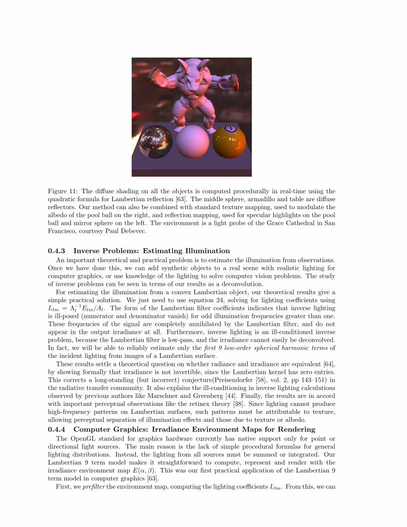
Figure 11: The diffuse shading on all the objects is computed procedurally in real-time using thequadratic formula for Lambertian reflection [63]. The middle sphere, armadillo and table are diffusereflectors. Our method can also be combined with standard texture mapping, used to modulate thealbedo of the pool ball on the right, and reflection mapping, used for specular highlights on the poolball and mirror sphere on the left. The environment is a light probe of the Grace Cathedral in SanFrancisco, courtesy Paul Debevec.

0.4.3 Inverse Problems: Estimating IlluminationAn important theoretical and practical problem is to estimate the illumination from observations.

Once we have done this, we can add synthetic objects to a real scene with realistic lighting forcomputer graphics, or use knowledge of the lighting to solve computer vision problems. The studyof inverse problems can be seen in terms of our results as a deconvolution.

For estimating the illumination from a convex Lambertian object, our theoretical results give asimple practical solution. We just need to use equation 24, solving for lighting coefficients usingLlm = Λ−1

l Elm/Al. The form of the Lambertian filter coefficients indicates that inverse lightingis ill-posed (numerator and denominator vanish) for odd illumination frequencies greater than one.These frequencies of the signal are completely annihilated by the Lambertian filter, and do notappear in the output irradiance at all. Furthermore, inverse lighting is an ill-conditioned inverseproblem, because the Lambertian filter is low-pass, and the irradiance cannot easily be deconvolved.In fact, we will be able to reliably estimate only the first 9 low-order spherical harmonic terms ofthe incident lighting from images of a Lambertian surface.

These results settle a theoretical question on whether radiance and irradiance are equivalent [64],by showing formally that irradiance is not invertible, since the Lambertian kernel has zero entries.This corrects a long-standing (but incorrect) conjecture(Preisendorfer [58], vol. 2, pp 143–151) inthe radiative transfer community. It also explains the ill-conditioning in inverse lighting calculationsobserved by previous authors like Marschner and Greenberg [44]. Finally, the results are in accordwith important perceptual observations like the retinex theory [38]. Since lighting cannot producehigh-frequency patterns on Lambertian surfaces, such patterns must be attributable to texture,allowing perceptual separation of illumination effects and those due to texture or albedo.

0.4.4 Computer Graphics: Irradiance Environment Maps for RenderingThe OpenGL standard for graphics hardware currently has native support only for point or

directional light sources. The main reason is the lack of simple procedural formulas for generallighting distributions. Instead, the lighting from all sources must be summed or integrated. OurLambertian 9 term model makes it straightforward to compute, represent and render with theirradiance environment map E(α, β). This was our first practical application of the Lambertian 9term model in computer graphics [63].

First, we prefilter the environment map, computing the lighting coefficients Llm. From this, we can

compute the 9 irradiance coefficients Elm per equation 24. This computation is very efficient, beinglinear in the size of the environment map. We can now adopt one of two approaches. The first is toexplicitly compute the irradiance map E(α, β) by evaluating it from the irradiance coefficients. Then,for any surface normal (α, β), we can simply look up the irradiance value and multiply by the albedoto shade the Lambertian surface. This was the approach taken in previous work on environmentmapping [21, 46]. Those methods needed to explicitly compute E(α, β) with a hemispherical integralof all the incident illumination for each surface normal. This was a slow procedure (it is O(n2) wheren is the size of the environment map in pixels). By contrast, our spherical harmonic prefilteringmethod is linear time O(n). Optimized implementations can run in near real-time, enabling ourmethod to potentially be used for dynamically changing illumination. Software for preconvolvingenvironment maps is available on our website and widely used by industry.

However, we can go much further than simply computing an explicit representation of E(α, β)quickly. In fact, we can use a simple procedural formula for shading. This allows us to avoid usingtextures for irradiance calculations. Further, the computations can be done at each vertex, insteadof at each pixel, since irradiance varies slowly. They are very simple to implement in either vertexshaders on the graphics card, or in software. All we need to do is explicitly compute

E(α, β) ≈2∑

l=0

l∑

m=−l

ElmYlm(α, β). (30)

This is straightforward, because the spherical harmonics up to order 2 are simply constant, linearand quadratic polynomials. In fact, we can write an alternative simple quadratic form,

E(n) = ntMn, (31)

where n is the 4× 1 surface normal in homogeneous cartesian coordinates and M is a 4× 4 matrix.Since this involves only a matrix-vector multiplication and dot-product, and hardware is optimizedfor these operations with 4 × 4 matrices and vectors, the calculation is very efficient. An explicitform for the matrix M is given in [63]. The image in figure 11 was rendered using this method,which is now widely adopted for real-time rendering in video games.

Note the duality between forward and inverse problems. The inverse problem, inverselighting, is ill-conditioned, with high frequencies of the lighting not easy to estimate. Conversely, theforward problem, irradiance environment maps, can be computed very efficiently, by approximatingonly the lowest frequencies of the illumination and irradiance. This duality between forward andinverse problems has rarely been used before, and we believe it can lead to many new applications.

0.5 Specularities: Convolution Formula for General MaterialsIn this section, we discuss the extension to general materials, including specularities, and briefly

explore the implications and practical applications of these general convolution results. We firstbriefly derive the fully general case with anisotropic materials [61, 67]. An illustrative diagram isfound in figure 12. For practical applications, it is often convenient to assume isotropic materials.The convolution result for isotropic BRDFs, along with implications are developed in [65, 67], andwe will quickly derive it here as a special case of the anisotropic theory.

0.5.1 General Convolution FormulaThe reflection equation, analogous to equation 8 in the Lambertian case, now becomes

B(α, β, γ, θ′o, φ′

o) =

∫

Ω′

i

L (Rα,β,γ (θ′i, φ′

i)) ρ(θ′i, φ′

i, θ′

o, φ′

o) dω′

i, (32)

where the reflected light field B now also depends on the (local) outgoing angles θ′

o, φ′

o. ρ is atransfer function (the BRDF multiplied by the cosine of the incident angle ρ = ρmax(cos θ′

i, 0)),which depends on local incident and outgoing angles.

The lighting can be expanded as per equations 19 and 20 in the Lambertian derivation. Theexpansion of the transfer function is now more general than equation 21, being given in spherical

)(

N

α

N

ο’θ ’

i

α

θ

B

i)(L

θο

θθ

θi

’θiθi

ο θi)(L

θο

LB )(

θi)(

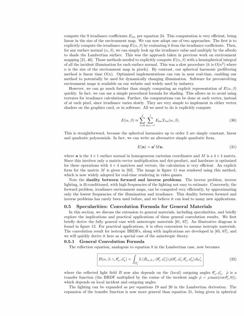
Figure 12: Schematic of reflection in 2D. On the left, we show the situation with respect to onepoint on the surface (the north pole or 0 location, where global and local coordinates are thesame). The right figure shows the effect of the surface orientation α. Different orientations ofthe surface correspond to rotations of the upper hemisphere and BRDF, with the global incidentdirection θi corresponding to a rotation by α of the local incident direction θ′

i. Note that we alsokeep the local outgoing angle (between N and B) fixed between the two figures.

harmonics by

ρ(θ′i, φ′

i, θ′

o, φ′

o) =

∞∑

l=0

l∑

n=−l

∞∑

p=0

p∑

q=−p

ρln,pqY∗

ln(θ′i, φ′

i)Ypq(θ′

o, φ′

o), (33)

where the complex conjugate for the first factor is to simplify the final results.Finally, we need to expand the reflected light field in basis functions. For the Lambertian case, we

simply used spherical harmonics over (α, β). In the general case, we must consider the full tangentframe (α, β, γ). Thus, the expansion is over mixed basis functions, Dl

mn(α, β, γ)Ypq(θ′

o, φ′

o). Withthe correct normalization(equation 7.73 of [28]),

B(α, β, γ, θ′o, φ′

o) =

∞∑

l=0

l∑

m=−l

l∑

n=−l

∞∑

p=0

p∑

q=−p

Blmn,pqClmn,pq(α, β, γ, θ′o, φ′

o)

Clmn,pq(α, β, γ, θ′o, φ′

o) =

√

2l + 1

8π2Dl

mn(α, β, γ)Ypq(θ′

o, φ′

o). (34)

We can now write down the reflection equation, as given by equation 32, in terms of the expansionsjust defined. As in the Lambertian case, we multiply the expansions for the lighting (equation 20)and BRDF (equation 33) and integrate. To avoid confusion between the indices in this intermediatestep, we will use Llm and ρl′n,pq to obtain

B(α, β, γ, θ′o, φ′

o) =

∞∑

l=0

l∑

m=−l

l∑

m′=−l

∞∑

l′=0

l′∑

n=−l′

∞∑

p=0

p∑

q=−p

Llmρl′n,pqDlmm′(α, β, γ)Ypq(θ

′

o, φ′

o)Tlm′l′n

Tlm′l′n =

∫ 2π

φ′

i=0

∫ π

θ′

i=0

Ylm′(θ′i, φ′

i)Y∗

l′n(θ′i, φ′

i) sin θ′i dθ′idφ′

i

= δll′δm′n. (35)

The last line follows from orthonormality of the spherical harmonics. Therefore, we may set l′ = land n = m′ since terms not satisfying these conditions vanish. We then obtain

B(α, β, γ, θ′o, φ′

o) =∞∑

l=0

l∑

m=−l

l∑

n=−l

∞∑

p=0

p∑

q=−p

Llmρln,pq

(

Dlmn(α, β, γ)Ypq(θ

′

o, φ′

o))

. (36)

Finally, equating coefficients, we obtain the spherical harmonic reflection equation or convolutionformula, analogous to equation 24. The reflected light field can be viewed as taking the incident

illumination signal, and filtering it with the material properties or BRDF of the surface,

Blmn,pq =

√

8π2

2l + 1Llmρln,pq. (37)

Isotropic BRDFs: An important special case are isotropic BRDFs, where the orientation of thelocal tangent frame γ does not matter. To consider the simplifications that result from isotropy, wefirst analyze the BRDF coefficients ρln,pq. In the BRDF expansion of equation 33, only terms thatsatisfy isotropy, i.e. are invariant with respect to adding an angle 4φ to both incident and outgoingazimuthal angles, are nonzero. From the form of the spherical harmonics, this requires that n = qand we write the now 3D BRDF coefficients as ρlpq = ρlq,pq.

Next, we remove the dependence of the reflected light field on γ by arbitrarily setting γ = 0. Thereflected light field can now be expanded in coefficients [65],

B(α, β, θ′o, φ′

o) =

∞∑

l=0

l∑

m=−l

∞∑

p=0

min(l,p)∑

q=−min(l,p)

BlmpqClmpq(α, β, θ′o, φ′

o)

Clmpq(α, β, θ′o, φ′

o) =

√

2l + 1

4πDl

mq(α, β, 0)Ypq(θ′

o, φ′

o). (38)

Finally, the convolution formula for isotropic BRDFs becomes

Blmpq = ΛlLlmρlpq. (39)

Finally, it is instructive to derive the Lambertian results as a special case of the above formulation.In this case, p = q = 0 (no exitant angular dependence), and equation 24 is effectively obtainedsimply by dropping the indices p and q in the above equation.

0.5.2 ImplicationsWe now briefly discuss the theoretical implications of these results. A more detailed discussion

can be found in [65, 67]. First, we consider inverse problems like illuminant and BRDF estimation.From the formula above, we can solve them simply by dividing the reflected light field coefficientsby the known lighting or BRDF coefficients, i.e. Llm = Λ−1

l Blmpq/ρlpq and ρlpq = Λ−1l Blmpq/Llm.

These problems will be well conditioned when the denominators do not vanish and contain highfrequency elements. In other words, for inverse lighting to be well conditioned, the BRDF shouldbe an all-pass filter, ideally a mirror surface. Mirrors are delta functions in the spatial or angulardomain, and include all frequencies in the spherical harmonic domain. Estimating the illuminationfrom a chrome-steel or mirror sphere is in fact a common approach. On the other hand, if the filteris low-pass, like a Lambertian surface, inverse lighting will be ill-conditioned. Similarly, for BRDFestimation to be well conditioned, the lighting should include high frequencies like sharp edges. Theideal is a directional or point light source. In fact, Lu et al. [41] and Marschner et al. [43] havedeveloped image-based BRDF measurement methods from images of a homogeneous sphere lit by apoint source. More recently, Gardner et al. [17] have used a linear light source. On the other hand,BRDF estimation is ill-conditioned under soft diffuse lighting. On a cloudy day, we will not be ableto estimate the widths of specular highlights accurately, since they will be blurred out.

Interesting special cases are Lambertian, and Phong and Torrance-Sparrow [77] BRDFs. We havealready discussed the Lambertian case in some detail. The frequency domain filters corresponding toPhong or microfacet models are approximately Gaussian [65]. In fact, the width of the Gaussian inthe frequency domain is inversely related to the width of the filter in the spatial or angular domain.The extreme cases are that of a mirror surface, that is completely localized (delta function) in theangular domain and passes through all frequencies (infinite frequency width), and of a very rough ornear-Lambertian surface that has full width in the angular domain, but is a very compact low-passfilter in the frequency domain. This duality between angular and frequency-space representationsis similar to that for Fourier basis functions. In some ways, it is also analogous to the Heisenberguncertainty principle—we cannot simultaneously localize a function in both angular and frequency

domains. For representation and rendering however, we can turn this to our advantage, usingeither the frequency or angular domain, wherever the different components of lighting and materialproperties can be more efficiently and compactly represented.

Another interesting theoretical question concerns factorization of the 4D reflected light field,simultaneously estimating the illumination (2D) and isotropic BRDF (3D). Since the lighting andBRDF are lower-dimensional entities, it seems that we have redundant information in the reflectedlight field. We show [65] that an analytic formula for both illumination and BRDF can be derivedfrom reflected light field coefficients. Thus, up to a global scale and possible ill-conditioning, thereflected light field can in theory be factored into illumination and BRDF components.

0.5.3 ApplicationsInverse Rendering: Inverse rendering refers to inverting the normal rendering process to es-timate illumination and materials from photographs. Many previous inverse rendering algorithmshave been limited to controlled laboratory conditions using point light sources. The insights from ourconvolution analysis have enabled the development of a general theoretical framework for handlingcomplex illumination. We [61, 65] have developed a number of frequency domain and dual angu-lar and frequency-domain algorithms for inverse rendering under complex illumination, includingsimultaneous estimation of the lighting and BRDFs from a small number of images.

Forward Rendering (Environment Maps with Arbitrary BRDFs): In the forward problem,all of the information on lighting and BRDFs is available, so we can directly apply the convolutionformula [66]. We have shown how this can be applied to rendering scenes with arbitrary distantillumination (environment maps) and BRDFs. As opposed to the Lambertian case, we no longer havea simple 9 term formula. However, just as in the Lambertian case, convolution makes prefilteringthe environment extremely efficient, three to four orders of magnitude faster than previous work.Furthermore, it allows us to use a new compact and efficient representation for rendering, theSpherical Harmonic Reflection Map or SHRM. The frequency domain analysis helps to precisely setthe number of terms and sampling rates and frequencies used for a given accuracy.

Material Representation and Recognition: Nillius and Eklundh [54, 55] derive a low-dimensional representation using PCA for images with complex lighting and materials. This can beseen as a generalization of the PCA results for diffuse surfaces (to which they have also made animportant contribution [53]). They can use these results to recognize or classify the materials in animage, based on their reflectance properties.

0.6 Relaxing and Broadening the Assumptions: Recent WorkSo far, we have seen how to model illumination, and the resulting variation in appearance of

objects using spherical harmonics. There remain a number of assumptions as far as the theoreticalconvolution analysis is concerned. Specifically, we assume distant lighting and convex objects withoutcast shadows or interreflections. Furthermore, we are dealing only with opaque objects in free space,and are not handling translucency or participating media. It has not so far been possible to extendthe theoretical analysis to relax these assumptions. However, a large body of recent theoretical andpractical work has indicated that the key concepts from the earlier analysis—such as convolution,filtering and spherical harmonics—can be used to analyze and derive new algorithms for all of theeffects noted above. The convolution formulas presented earlier in the chapter will of course nolonger hold, but the insights can be seen to be much more broadly applicable.

Cast Shadows: For certain special cases, it is possible to derive a convolution result for castshadows (though not in terms of spherical harmonics). For parallel planes, Soler and Sillion [75]have derived a convolution result, using it as a basis for a fast algorithm for soft shadows. We [68]have developed a similar result for V-grooves to explain lighting variability in natural 3D textures.

An alternative approach is to incorporate cast shadows in the integrand of the reflection equation.The integral then includes three terms, instead of two—the illumination, the BRDF (or Lambertianhalf-cosine function), and a binary term for cast shadows. Since cast shadows vary spatially, reflectionis no longer a convolution in the general case. However, it is still possible to use spherical harmonics

to represent the terms of the integrand. Three term or triple product integrals can be analyzedusing the Clebsch-Gordan series for spherical harmonics [28], that is common for analyzing angularmomentum in quantum mechanics. A start at working out the theory is made by Thornber andJacobs [76]. Most recently, we [51] have investigated generalizations of the Clebsch-Gordan seriesfor other bases, like Haar wavelets, in the context of real-time rendering with cast shadows.

Pre-Computed Light Transport: Sloan et al. [74] recently introduced a new approach to real-time rendering called precomputed radiance transfer. Their method uses low-frequency sphericalharmonic representations (usually order 4 or 25 terms) of the illumination and BRDF, and allowsfor a number of complex light-transport effects including soft shadows, interreflections, global il-lumination effects like caustics, and dynamically changing lighting and viewpoint. Because of thehigh level of realism these approaches provide compared to standard hardware rendering, sphericalharmonic lighting is now widely used in interactive applications like video games, and is incorporatedinto Microsoft’s DirectX API.

We introduce the theory only for Lambertian surfaces—relatively straightforward extensions arepossible for complex materials, including view-dependence. The basic idea is to define a transportoperator T that includes half-cosine, visibility and interreflection effects. We can then write, inanalogy with equations 3 and 6,

E(x) =

∫

Ωi

L(ωi)T (x,ωi) dωi, (40)

where T denotes the irradiance at x due to illumination from direction ωi, and incorporates alllight-transport effects including cast shadows and interreflections. An offline precomputation step(that may involve ray-tracing for instance) is used to determine T for a static scene. We can expandall quantities in spherical harmonics, to write

E(x) ≈l∗∑

l=0

l∑

m=−l

Tlm(x)Llm, (41)

where l∗ denotes the maximum order used for calculations (2 would be sufficient in the absence of castshadows). We repeat this calculation for each vertex x for rendering. The expression above is simplya dot product which can be implemented efficiently in current programmable graphics hardware,allowing real-time manipulation of illumination. Somewhat more complicated, but conceptuallysimilar expressions, are available for glossy materials. For real-time rendering with varying lightingand viewpoint, Sloan et al. [73] precompute a view-dependent operator (a 25×25 matrix of sphericalharmonic coefficients at each vertex) and compress the information over the surface using clusteredprincipal component analysis.

New Basis Functions: Spherical harmonics are the ideal signal-processing representation whenwe have a convolution formula or want to analyze functions in the frequency domain. However,they are not the best representation for “all-frequency” effects—an infinite number of sphericalharmonics will be needed to accurately represent a point source or delta function. Furthermore,some quantities like the BRDF are better defined over the hemisphere rather than the full sphere. Incases where cast shadows and interreflections are involved, we no longer have a convolution formula,so spherical harmonics are sometimes not the preferred representation. Recently, we [50, 51] haveintroduced all-frequency relighting methods using Haar wavelets. These methods can be ordersof magnitude more efficient than previous precomputed light transport techniques using sphericalharmonics. Hemispherical basis functions for BRDF representation have been proposed by Gautronet al. [18] and Koenderink and van Doorn [36].

Near-Field Illumination: Recent theoretical work [16] has tried to remove the limitation ofdistant illumination, by showing a convolution result (with a different kernel) to also hold for near-field lighting under specific assumptions for Lambertian surfaces. A practical solution using sphericalharmonic gradients for rendering is proposed by Annen et al. [1].

Translucency and Participating Media: Like most of computer vision and graphics, we haveso far assumed clear-day conditions, without translucent materials like marble and skin, or partici-pating media like milk, smoke, clouds or fog. Both spherical harmonics and convolution are populartools for subsurface scattering, volumetric rendering and radiative transport problems. Practicalmethods that conceptually use convolution of the incident irradiance with a point-spread functionhave been employed successfully for subsurface scattering [30, 31], and we have recently developedsuch methods for rendering multiple scattering effects in volumetric participating media [49, 59].

0.7 ConclusionMuch of the richness of the visual appearance of our world arises from the effects of illumination,

and the varying appearance of surfaces with lighting. In this chapter, we have seen that there aremany situations in the real world, such as for diffuse Lambertian surfaces, where the appearanceof an object can be relatively simple to describe, even if the lighting is complicated. We haveintroduced new tools to model illumination and appearance using spherical harmonics. With thesetools, we can derive a signal-processing approach to reflection, where the reflected light can bethought of as obtained by filtering or convolving the incident illumination signal by the materialproperties of the surface. This insight leads to a number of new results, and explanations of previousexperimental work, such as the 9 parameter low-dimensional subspace for Lambertian objects. Thereare implications for face modeling, recognition and rendering, as well as a number of other problemsin computer vision, graphics and perception. Already, a number of new algorithms have beendeveloped in computer vision for recognition and modeling, and in computer graphics for bothforward and inverse problems in rendering, with the promise of many further developments in thenear future.

Acknowledgements: Special thanks to all my co-authors and collaborators, with particulargratitude to Pat Hanrahan, David Jacobs, Ronen Basri and Ren Ng. This work was supported inpart by grants #0305322, #0430258 and #0446916 from the National Science Foundation and fromIntel Corporation.

Bibliography

[1] T. Annen, J. Kautz, F. Durand, and H. Seidel. Spherical harmonic gradients for mid-range illumination.In EuroGraphics Symposium on Rendering, 2004.

[2] R. Basri and D. Jacobs. Lambertian reflectance and linear subspaces. In International Conference onComputer Vision, pages 383–390, 2001.

[3] R. Basri and D. Jacobs. Photometric stereo with general, unknown lighting. In CVPR 01, pagesII–374–II–381, 2001.

[4] R. Basri and D. Jacobs. Lambertian reflectance and linear subspaces. PAMI, 25(2):218–233, 2003.

[5] R. Basri and D. Jacobs. Illumination Modeling for Face Recognition, chapter 5, Face RecognitionHandbook. Springer Verlag, 2004.

[6] P. Belhumeur and D. Kriegman. What is the set of images of an object under all possible illuminationconditions? IJCV, 28(3):245–260, 1998.

[7] J. Blinn and M. Newell. Texture and reflection in computer generated images. Communications of theACM, 19:542–546, 1976.

[8] R. Brunelli and T. Poggio. Face recognition: Features versus templates. IEEE Transactions on PatternAnalysis and Machine Intelligence, 15(10):1042–1062, 1993.

[9] B. Cabral, N. Max, and R. Springmeyer. Bidirectional reflection functions from surface bump maps. InSIGGRAPH 87, pages 273–281, 1987.

[10] B. Cabral, M. Olano, and P. Nemec. Reflection space image based rendering. In SIGGRAPH 99, pages165–170, 1999.

[11] H. Chen, P. Belhumeur, and D. Jacobs. In search of illumination invariants. In CVPR 00, pages254–261, 2000.

[12] M. Cohen and J. Wallace. Radiosity and Realistic Image Synthesis. Academic Press, 1993.

[13] P. Debevec, T. Hawkins, C. Tchou, H.P. Duiker, W. Sarokin, and M. Sagar. Acquiring the reflectancefield of a human face. In SIGGRAPH 00, pages 145–156, 2000.

[14] M. D’Zmura. Computational Models of Visual Processing, chapter Shading Ambiguity: Reflectance andIllumination, pages 187–207. MIT Press, 1991.

[15] R. Epstein, P.W. Hallinan, and A. Yuille. 5 plus or minus 2 eigenimages suffice: An empirical investi-gation of low-dimensional lighting models. In IEEE Workshop on Physics-Based Modeling in ComputerVision, pages 108–116, 1995.

[16] D. Frolova, D. Simakov, and R. Basri. Accuracy of spherical harmonic approximations for images oflambertian objects under far and near lighting. In ECCV, pages I–574–I–587, 2004.

[17] A. Gardner, C. Tchou, T. Hawkins, and P. Debevec. Linear light source reflectometry. ACM TOG(SIGGRAPH 2003), 22(3):749–758, 2003.

[18] P. Gautron, J. Krivanek, S. Pattanaik, and K. Bouatouch. A novel hemispherical basis for accurateand efficient rendering. In EuroGraphics Symposium on Rendering, 2004.

[19] A. Georghiades, P. Belhumeur, and D. Kriegman. From few to many: Generative models for recognitionunder variable pose and illumination. In Fourth International Conference on Automatic Face andGuesture Recogniton, pages 277–284, 2000.

[20] A. Georghiades, D. Kriegman, and P. Belhumeur. Illumination cones for recognition under variablelighting: Faces. In CVPR 98, pages 52–59, 1998.

[21] N. Greene. Environment mapping and other applications of world projections. IEEE Computer Graphics& Applications, 6(11):21–29, 1986.

25

[22] H. Groemer. Geometric applications of Fourier series and spherical harmonics. Cambridge UniversityPress, 1996.

[23] P.W. Hallinan. A low-dimensional representation of human faces for arbitrary lighting conditions. InCVPR 94, pages 995–999, 1994.

[24] H. Hayakawa. Photometric stereo under a light source with arbitrary motion. Journal of the OpticalSociety of America A, 11(11):3079–3089, Nov 1994.

[25] W. Heidrich and H. P. Seidel. Realistic, hardware-accelerated shading and lighting. In SIGGRAPH 99,pages 171–178, 1999.

[26] J. Ho, M. Yang, J. Lim, K. Lee, and D. Kriegman. Clustering appearances of objects under varyingillumination conditions. In CVPR, volume 1, pages 11–18, 2003.

[27] B. Horn. Robot Vision. MIT Press, 1986.

[28] T. Inui, Y. Tanabe, and Y. Onodera. Group theory and its applications in physics. Springer Verlag,1990.

[29] J. Jackson. Classical Electrodynamics. John Wiley, 1975.

[30] H. Jensen and J. Buhler. A rapid hierarchical rendering technique for translucent materials. ACMTransactions on Graphics (SIGGRAPH 2002), 21(3):576–581, 2002.

[31] H. Jensen, S. Marschner, M. Levoy, and P. Hanrahan. A practical model for subsurface light transport.In SIGGRAPH 2001, pages 511–518, 2001.

[32] J. Kautz and M. McCool. Approximation of glossy reflection with prefiltered environment maps. InGraphics Interface, pages 119–126, 2000.

[33] J. Kautz, P. Vazquez, W. Heidrich, and H.P. Seidel. A unified approach to prefiltered environmentmaps. In Eurographics Rendering Workshop 00, pages 185–196, 2000.

[34] M. Kirby and L. Sirovich. Application of the Karhunen-Loeve procedure for the characterization ofhuman faces. PAMI, 12(1):103–108, Jan 1990.

[35] J. Koenderink and A. van Doorn. The generic bilinear calibration-estimation problem. IJCV, 23(3):217–234, 1997.

[36] J. Koenderink and A. van Doorn. Phenomenological description of bidirectional surface reflection.JOSA A, 15(11):2903–2912, 1998.

[37] M. Lades, J. Vorbruggen, J. Buhmann, J. Lange, C. von der Malsburg, R. Wurtz, and W. Konen. Dis-tortion invariant object recognition in the dynamic link architecture. IEEE Transactions on Computers,42(3):300–311, 1992.

[38] E. Land and J. McCann. Lightness and retinex theory. Journal of the Optical Society of America,61(1):1–11, 1971.

[39] K. Lee, J. Ho, and D. Kriegman. Nine points of light: Acquiring subspaces for face recognition undervariable lighting. In CVPR, pages 519–526, 2001.

[40] A. Levin and A. Shashua. Principal component analysis over continuous subspaces and intersection ofhalf-spaces. In To appear, ECCV 02, 2002.

[41] R. Lu, J.J. Koenderink, and A.M.L. Kappers. Optical properties (bidirectional reflection distributionfunctions) of velvet. Applied Optics, 37(25):5974–5984, 1998.

[42] T. MacRobert. Spherical harmonics; an elementary treatise on harmonic functions, with applications.Dover Publications, 1948.

[43] S. Marschner, S. Westin, E. Lafortune, and K. Torrance. Image-Based BRDF measurement. AppliedOptics, 39(16):2592–2600, 2000.

[44] S.R. Marschner and D.P. Greenberg. Inverse lighting for photography. In Fifth Color Imaging Confer-ence, pages 262–265, 1997.

[45] R. McCluney. Introduction to Radiometry and Photometry. Artech House, 1994.

[46] G. Miller and C. Hoffman. Illumination and reflection maps: Simulated objects in simulated and realenvironments. SIGGRAPH 84 Advanced Computer Graphics Animation seminar notes, 1984.

[47] Y. Moses, Y. Adini, and S. Ullman. Face recognition: the problem of compensating for changes inillumination direction. In ECCV 94, pages 286–296, 1994.

[48] H. Murase and S. Nayar. Visual learning and recognition of 3-D objects from appearance. IJCV,14(1):5–24, 1995.

[49] S. Narasimhan, R. Ramamoorthi, and S. Nayar. Analytic rendering of multiple scattering in partici-pating media. Submitted to ACM Transactions on Graphics, 2004.

[50] R. Ng, R. Ramamoorthi, and P. Hanrahan. All-frequency shadows using non-linear wavelet lightingapproximation. ACM Transactions on Graphics (SIGGRAPH 2003), 22(3), 2003.

[51] R. Ng, R. Ramamoorthi, and P. Hanrahan. Triple product wavelet integrals for all-frequency relighting.ACM Transactions on Graphics (SIGGRAPH 2004), 23(3):475–485, 2004.

[52] F. E. Nicodemus, J. C. Richmond, J. J. Hsia, I. W. Ginsberg, and T. Limperis. Geometric Considerationsand Nomenclature for Reflectance. National Bureau of Standards (US), 1977.

[53] P. Nillius and J. Eklundh. Low-dimensional representations of shaded surfaces under varying illumina-tion. In CVPR 03, pages II:185–II:192, 2003.

[54] P. Nillius and J. Eklundh. Phenomenological eigenfunctions for irradiance. In ICCV 03, pages I:568–I:575, 2003.

[55] P. Nillius and J. Eklundh. Classifying materials from their reflectance properties. In ECCV 04, pagesIV–366–IV–376, 2004.

[56] J. Nimeroff, E. Simoncelli, and J. Dorsey. Efficient re-rendering of naturally illuminated environments.In Eurographics Workshop on Rendering 94, pages 359–373, June 1994.

[57] M. Osadchy, D. Jacobs, and R. Ramamoorthi. Using specularities for recognition. In ICCV, pages1512–1519, 2003.

[58] R.W. Preisendorfer. Hydrologic Optics. US Dept Commerce, 1976.

[59] S. Premoze, M. Ashikhmin, R. Ramamoorthi, and S. Nayar. Practical rendering of multiple scatteringeffects in participating media. In EuroGraphics Symposium on Rendering, 2004.

[60] R. Ramamoorthi. Analytic PCA construction for theoretical analysis of lighting variability in imagesof a Lambertian object. IEEE Transactions on Pattern Analysis and Machine Intelligence (PAMI),24(10):1322–1333, Oct 2002.

[61] R. Ramamoorthi. A Signal-Processing Framework for Forward and Inverse Rendering. PhD thesis,Stanford University, 2002.

[62] R. Ramamoorthi and P. Hanrahan. Analysis of planar light fields from homogeneous convex curvedsurfaces under distant illumination. In SPIE Photonics West: Human Vision and Electronic ImagingVI, pages 185–198, 2001.

[63] R. Ramamoorthi and P. Hanrahan. An efficient representation for irradiance environment maps. InSIGGRAPH 01, pages 497–500, 2001.

[64] R. Ramamoorthi and P. Hanrahan. On the relationship between radiance and irradiance: Determiningthe illumination from images of a convex lambertian object. Journal of the Optical Society of AmericaA, 18(10):2448–2459, 2001.

[65] R. Ramamoorthi and P. Hanrahan. A signal-processing framework for inverse rendering. In SIGGRAPH01, pages 117–128, 2001.

[66] R. Ramamoorthi and P. Hanrahan. Frequency space environment map rendering. ACM Transactionson Graphics (SIGGRAPH 02 proceedings), 21(3):517–526, 2002.

[67] R. Ramamoorthi and P. Hanrahan. A signal-processing framework for reflection. ACM Transactionson Graphics, 23(4):1004–1042, 2004.

[68] R. Ramamoorthi, M. Koudelka, and P. Belhumeur. A fourier theory for cast shadows. IEEE Transac-tions on Pattern Analysis and Machine Intelligence, 27(2):288–295, 2005.

[69] A. Shashua. On photometric issues in 3D visual recognition from a single 2D image. IJCV, 21:99–122,1997.

[70] F. Sillion, J. Arvo, S. Westin, and D. Greenberg. A global illumination solution for general reflectancedistributions. In SIGGRAPH 91, pages 187–196, 1991.

[71] D. Simakov, D. Frolova, and R. Basri. Dense shape reconstruction of a moving object under arbitrary,unknown lighting. In ICCV 03, pages 1202–1209, 2003.

[72] L. Sirovich and M. Kirby. Low-dimensional procedure for the characterization of human faces. JOSAA, 4(3):519–524, Mar 1987.

[73] P. Sloan, J. Hall, J. Hart, and J. Snyder. Clustered principal components for precomputed radiancetransfer. ACM Transactions on Graphics (SIGGRAPH 03 proceedings), 22(3), 2002.

[74] P. Sloan, J. Kautz, and J. Snyder. Precomputed radiance transfer for real-time rendering in dynamic,low-frequency lighting environments. ACM Transactions on Graphics (SIGGRAPH 02 proceedings),21(3):527–536, 2002.

[75] C. Soler and F. Sillion. Fast calculation of soft shadow textures using convolution. In SIGGRAPH 98,pages 321–332, 1998.

[76] K. Thornber and D. Jacobs. Broadened, specular reflection and linear subspaces. Technical ReportTR#2001-033, NEC, 2001.

[77] K. Torrance and E. Sparrow. Theory for off-specular reflection from roughened surfaces. JOSA,57(9):1105–1114, 1967.

[78] M. Turk and A. Pentland. Eigenfaces for recognition. Journal of Cognitive Neuroscience, 3(1):71–96,1991.

[79] S. Westin, J. Arvo, and K. Torrance. Predicting reflectance functions from complex surfaces. InSIGGRAPH 92, pages 255–264, 1992.

[80] A. Yuille, D. Snow, R. Epstein, and P. Belhumeur. Determining generative models of objects undervarying illumination: Shape and albedo from multiple images using SVD and integrability. IJCV,35(3):203–222, 1999.

[81] L. Zhang, B. Curless, A. Hertzmann, and S. Seitz. Shape and motion under varying illumination:Unifying multiview stereo, photometric stereo, and structure from motion. In International Conferenceon Computer Vision, pages 618–625, 2003.

[82] L. Zhang and D. Samaras. Face recognition under variable lighting using harmonic image exemplars.In CVPR, pages I:19–I:25, 2003.

[83] L. Zhao and Y. Yang. Theoretical analysis of illumination in PCA-based vision systems. PatternRecognition, 32:547–564, 1999.