Modeling Latent Variable Uncertainty for Loss-based Learning Daphne Koller Stanford Universit Ben Packer tanford University M. Pawan Kumar École Centrale Paris École des Ponts ParisTech INRIA Saclay, Île-de-France
Transcript
Modeling Latent Variable Uncertainty for Loss-based Learning
Daphne KollerStanford University
Ben PackerStanford University
M. Pawan KumarÉcole Centrale Paris
École des Ponts ParisTechINRIA Saclay, Île-de-France
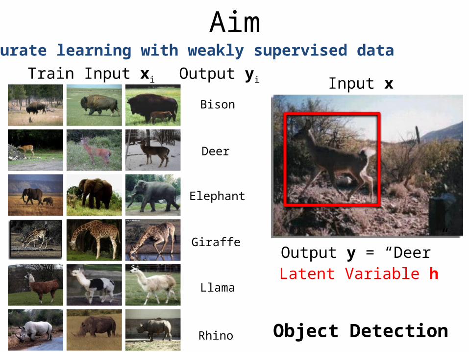
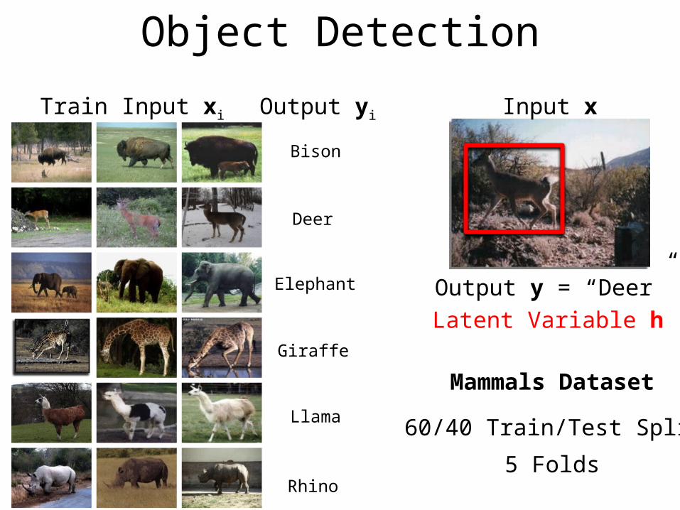
AimAccurate learning with weakly supervised data
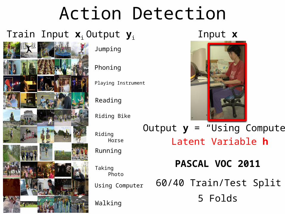
Train Input xi Output yi
Bison
Deer
Elephant
Giraffe
Llama
Rhino Object Detection
Input x
Output y = “Deer”Latent Variable h
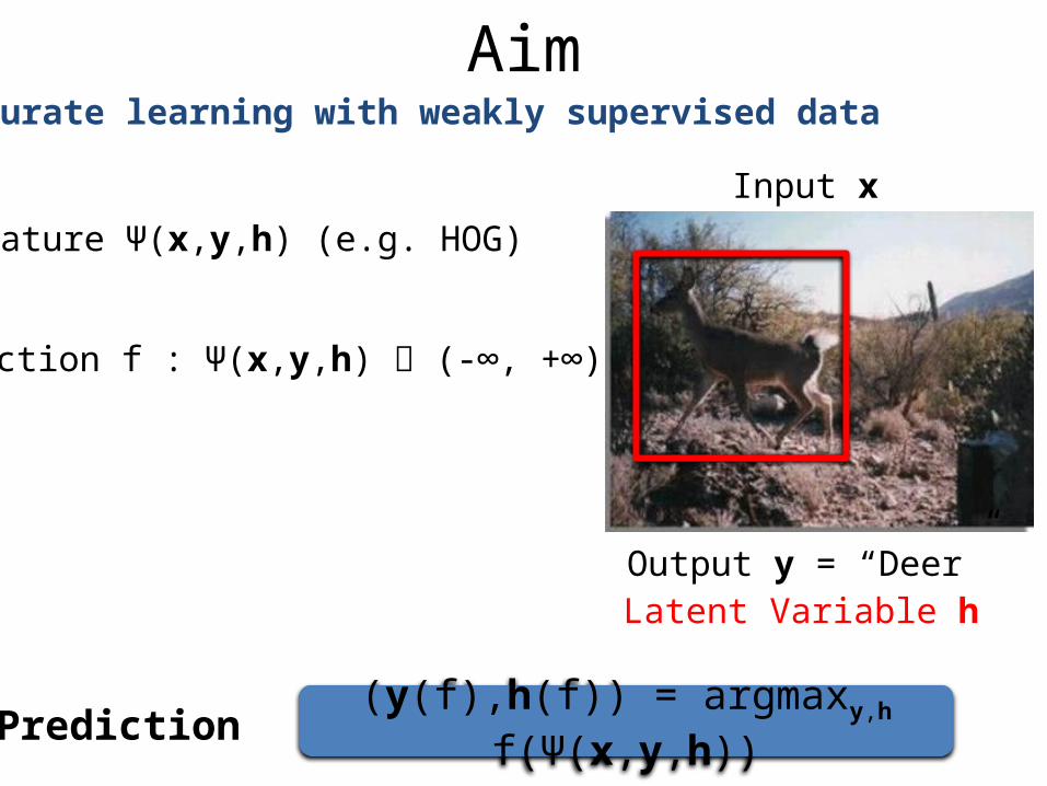
(y(f),h(f)) = argmaxy,h f(Ψ(x,y,h))
AimAccurate learning with weakly supervised data
Feature Ψ(x,y,h) (e.g. HOG)
Input x
Output y = “Deer”
Prediction
Function f : Ψ(x,y,h) (-∞, +∞)
Latent Variable h
f* = argminf Objective(f)
AimAccurate learning with weakly supervised data
Feature Ψ(x,y,h) (e.g. HOG)
Input x
Output y = “Deer”
Function f : Ψ(x,y,h) (-∞, +∞)
Learning
Latent Variable h
AimFind a suitable objective function to learn f*
Feature Ψ(x,y,h) (e.g. HOG)
Input x
Output y = “Deer”
Function f : Ψ(x,y,h) (-∞, +∞)
Learning
Encourages accurate prediction
User-specified criterion for accuracy
f* = argminf Objective(f)
Latent Variable h
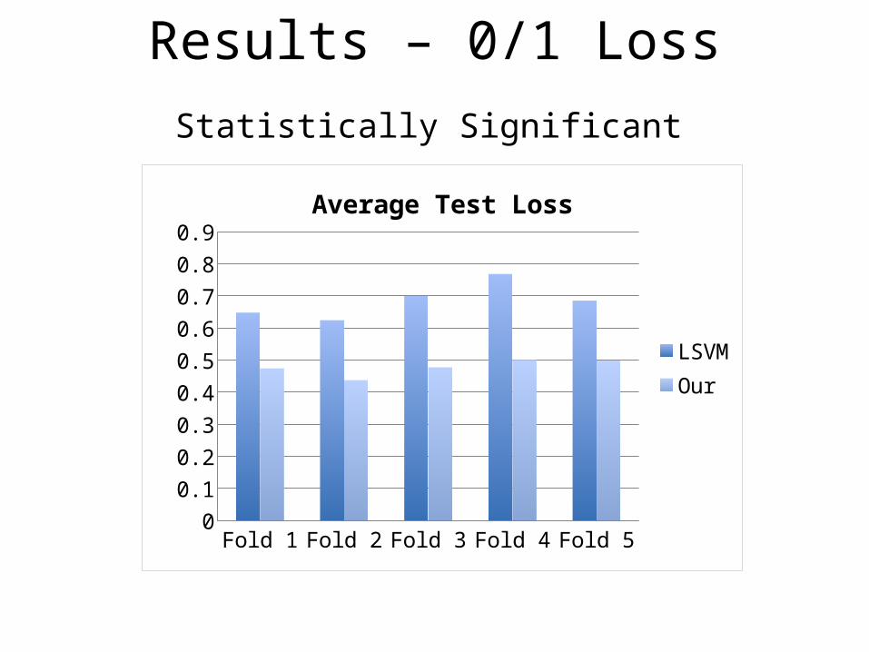
• Previous Methods
• Our Framework
• Optimization
• Results
• Ongoing and Future Work
Outline
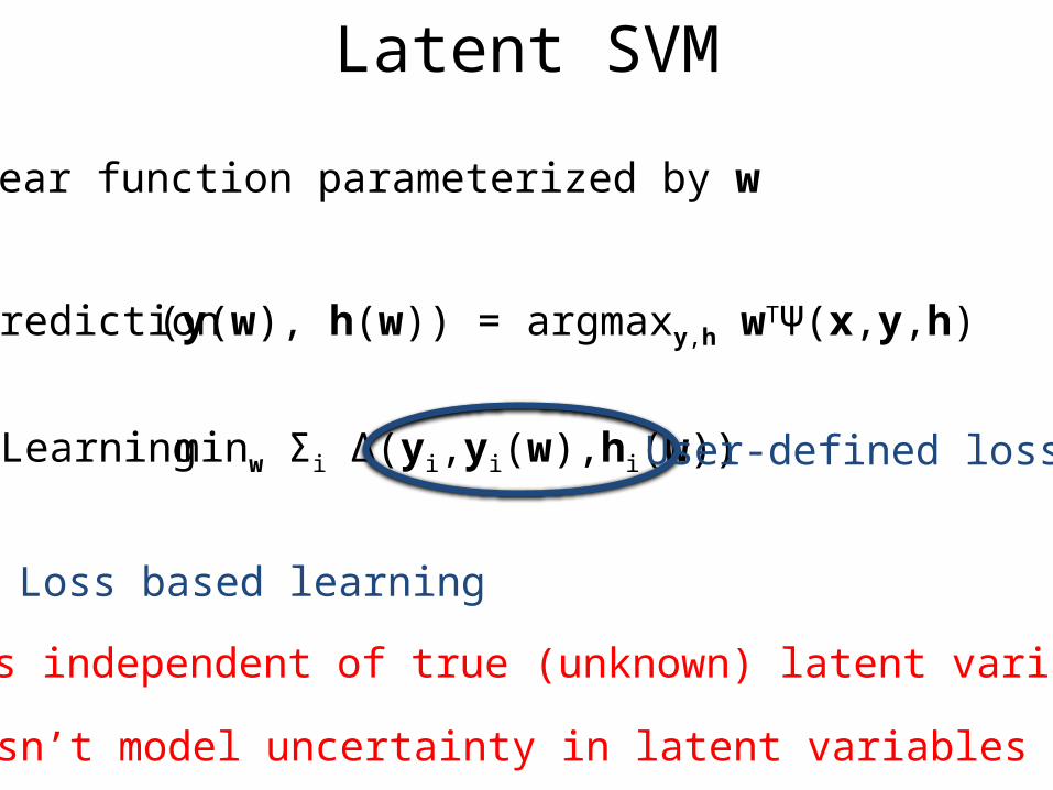
Latent SVM
Linear function parameterized by w
Prediction (y(w), h(w)) = argmaxy,h wTΨ(x,y,h)
Learning minw Σi Δ(yi,yi(w),hi(w))
✔ Loss based learning
✖ Loss independent of true (unknown) latent variable
✖ Doesn’t model uncertainty in latent variables
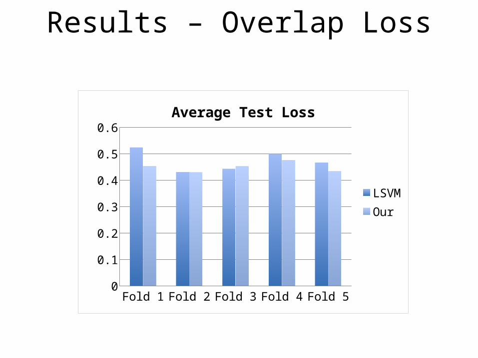
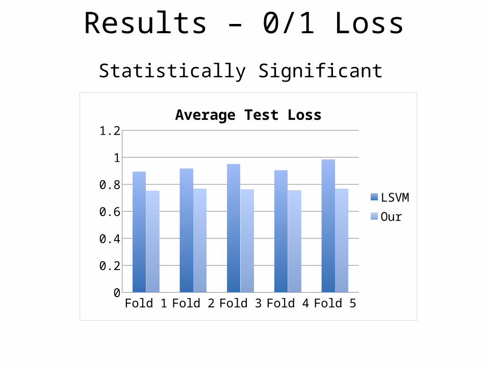
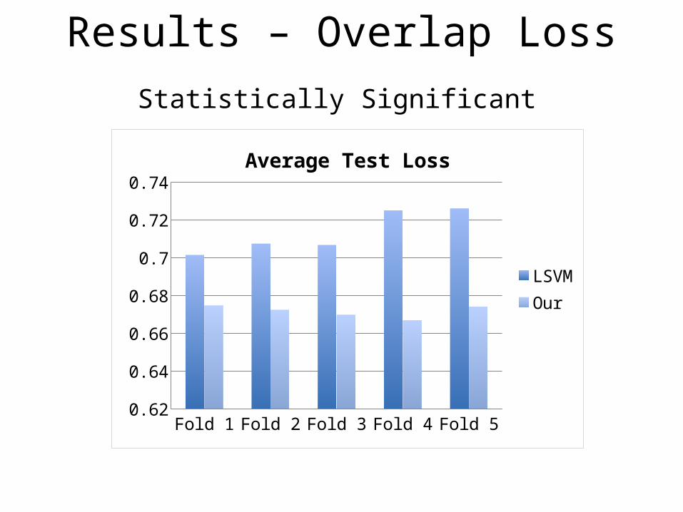
User-defined loss
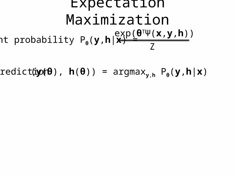
Expectation Maximization
Joint probability Pθ(y,h|x) =exp(θTΨ(x,y,h))
Z
Prediction (y(θ), h(θ)) = argmaxy,h Pθ(y,h|x)
Expectation Maximization
Joint probability Pθ(y,h|x) =exp(θTΨ(x,y,h))
Z
Prediction (y(θ), h(θ)) = argmaxy,h θTΨ(x,y,h)
Learning maxθ Σi log (Pθ(yi|xi))
Expectation Maximization
Joint probability Pθ(y,h|x) =exp(θTΨ(x,y,h))
Z
Prediction (y(θ), h(θ)) = argmaxy,h θTΨ(x,y,h)
Learning maxθ Σi Σhi log (Pθ(yi,hi|xi))
✔ Models uncertainty in latent variables
✖ Doesn’t model accuracy of latent variable prediction
✖ No user-defined loss function
• Previous Methods
• Our Framework
• Optimization
• Results
• Ongoing and Future Work
Outline
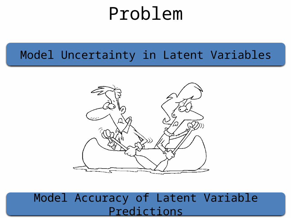
Problem
Model Uncertainty in Latent Variables
Model Accuracy of Latent Variable Predictions
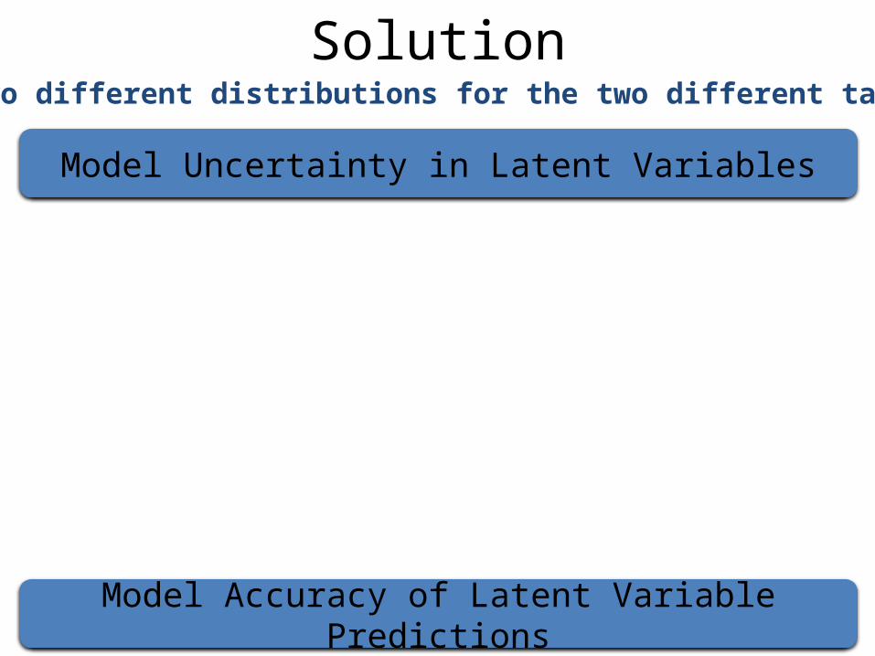
Solution
Model Uncertainty in Latent Variables
Model Accuracy of Latent Variable Predictions
Use two different distributions for the two different tasks
Solution
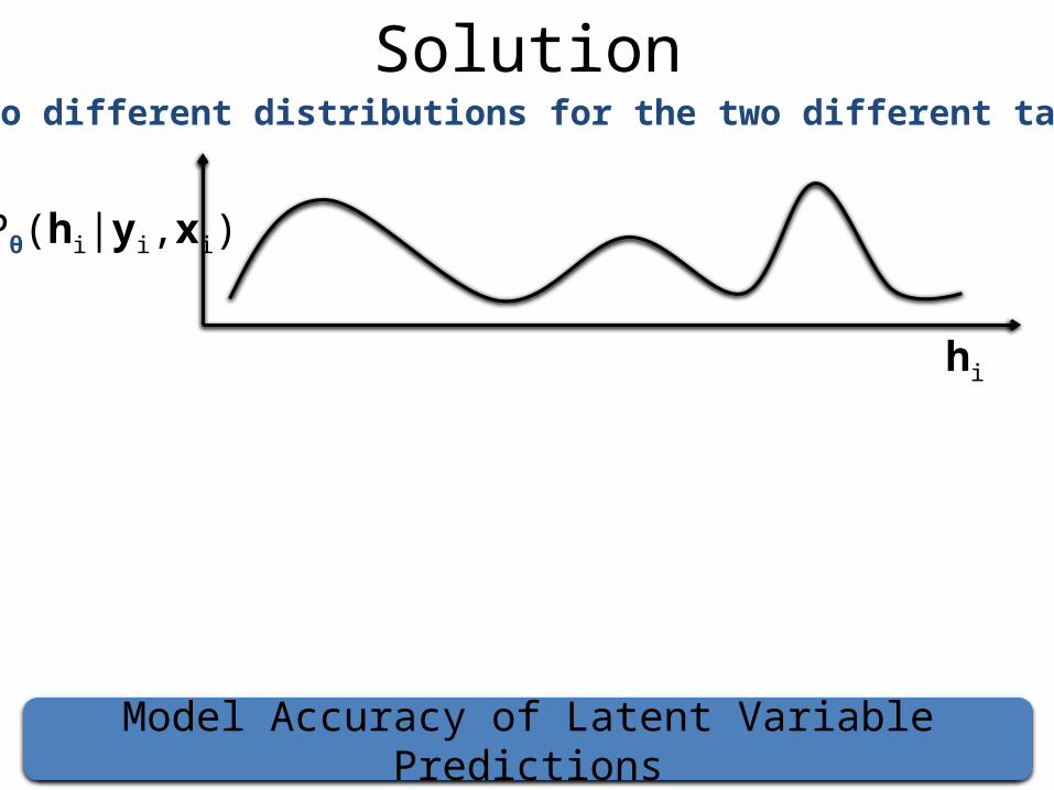
Model Accuracy of Latent Variable Predictions
Use two different distributions for the two different tasks
Pθ(hi|yi,xi)
hi
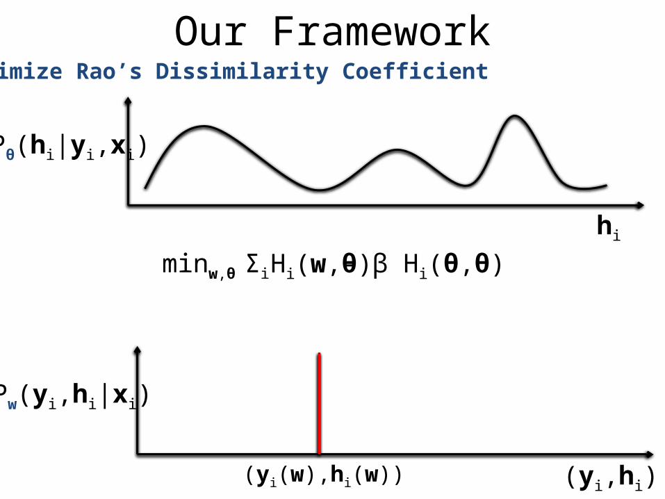
SolutionUse two different distributions for the two different tasks
hi
Pw(yi,hi|xi)
(yi,hi)(yi(w),hi(w))
Pθ(hi|yi,xi)
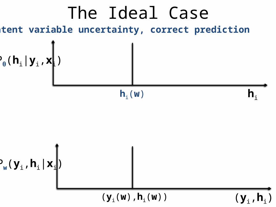
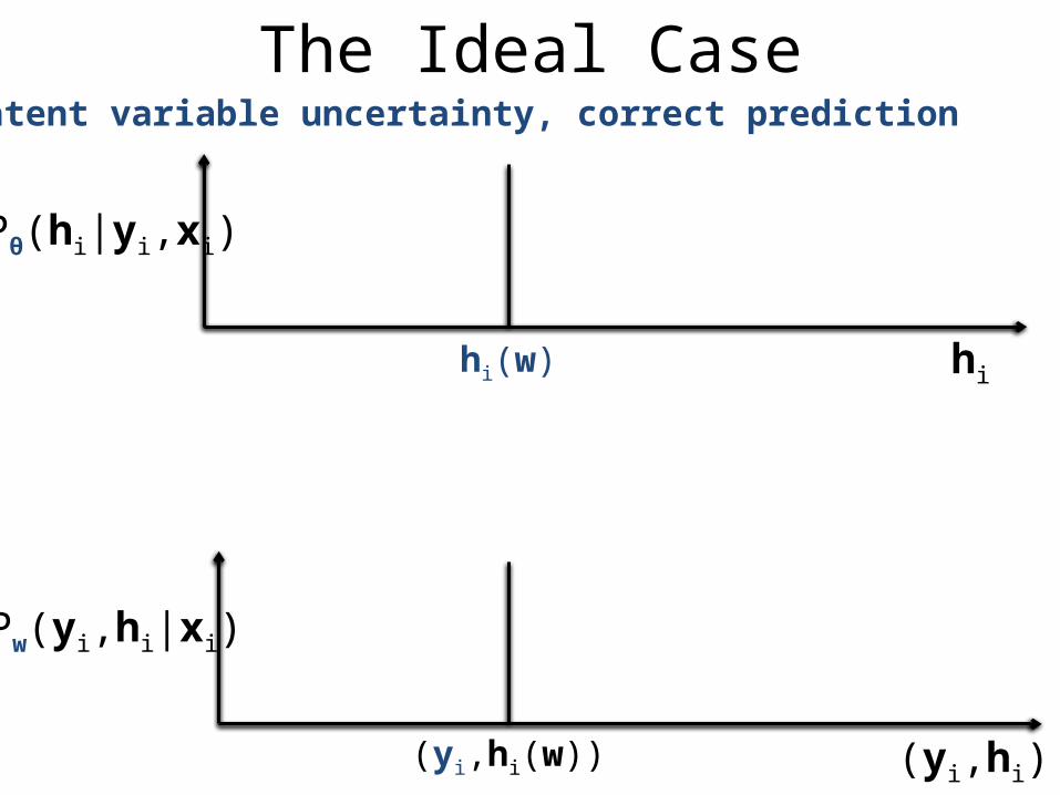
The Ideal CaseNo latent variable uncertainty, correct prediction
hi
Pw(yi,hi|xi)
(yi,hi)(yi(w),hi(w))
Pθ(hi|yi,xi)
The Ideal CaseNo latent variable uncertainty, correct prediction
hi
Pw(yi,hi|xi)
(yi,hi)(yi(w),hi(w))
Pθ(hi|yi,xi)
hi(w)
The Ideal CaseNo latent variable uncertainty, correct prediction
hi
Pw(yi,hi|xi)
(yi,hi)(yi,hi(w))
Pθ(hi|yi,xi)
hi(w)
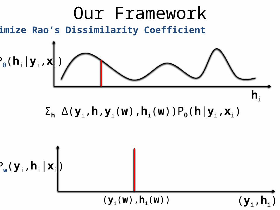
In PracticeRestrictions in the representation power of models
hi
Pw(yi,hi|xi)
(yi,hi)(yi(w),hi(w))
Pθ(hi|yi,xi)
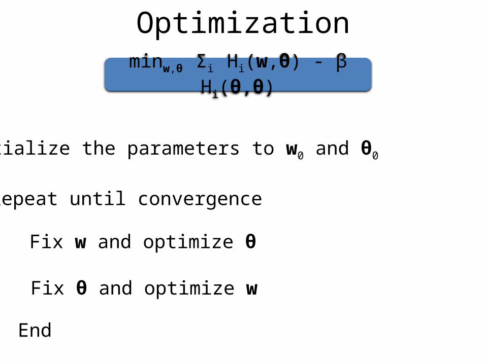
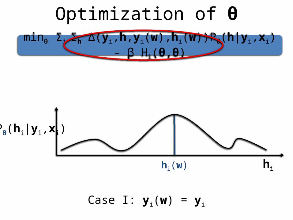
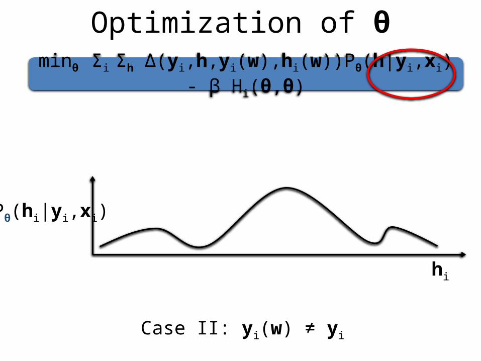
Our FrameworkMinimize the dissimilarity between the two distributions


![EMPA Koller[1]](https://static.documents.pub/doc/80x56/577ccf8e1a28ab9e789008fa/empa-koller1.jpg)


