Pure appl. geophys. 150 (1997) 217–2480033–4553/97/020217–32 $ 1.50+0.20/0

Modeling Low-frequency Magnetic-field Precursors to the LomaPrieta Earthquake with a Precursory Increase in Fault-zone

Conductivity

MOSHE MERZER1 and SIMON L. KLEMPERER2

Abstract—The 1989 Ms=7.1 Loma Prieta earthquake was preceded for 12 days by what have beenclaimed as precursory ultra-low-frequency (ULF) magnetic noise anomalies ten times background, andby a very high peak up to 100 times background just 3 hours before the earthquake. We propose thatthese anomalous fields could have been due to the formation of a long thin highly-conductive region alongthe earthquake fault, which magnified the external electromagnetic waves incident on the earth’s surface.We use a simplified quantitative model, assuming a highly-conductive elliptic cylinder embedded in alayered resistivity structure, which we base on independent magnetotelluric measurements. The magnetic-field anomaly observed 3 hours before the main shock can be modeled by assuming an elliptic conductorextending from the surface to the hypocenter with a conductivity of 5 S · m−1. Our computed anomalymatches the observed anomaly to within a deviation of 35% over an observed frequency range of over2 orders of magnitude, over which the measured anomaly varies from only about twice background (at5 Hz) to about 100 times background (at 0.01 Hz). In addition, other anomalies recorded up to 12 daysbefore the earthquake, can be modeled in detail by varying only the size of the elliptic conductor.

We show that such an increase in conductivity could be caused by a precursory reorganization ofthe geometry of fluid-filled porosity in the fault-zone, which we call a dilatant-conductive effect. Theextreme observed magnetic anomalies can be modeled using the high fault-zone porosity (c. 10%) and fluidconductivity (equivalent to 2 M NaCl) implied by other workers’ magneto-telluric measurements, butwithout requiring the large-scale precursory fluid flow characteristic of other published models for themagnetic-field precursors.

Key words: Earthquake precursors, Loma Prieta earthquake, fault zones, crustal fluids, electromag-netic theory, crustal conductivity.

Introduction

Scope of this Paper

It is impossible to demonstrate that any claimed earthquake precursor was trulyprecursory, that is, forewarning of, rather than merely prior to, the earthquake,because the earthquakes and anomalies cannot be experimentally generated. Onemust judge the claim that a measured anomaly was an earthquake precursor in two

1 RAFAEL, Electromagnetics Dept., P.O. Box 2250 (87), Haifa 31021, Israel.2 Department of Geophysics, Mitchell Building, Stanford University, Stanford CA 94305-2215,

U.S.A. Fax: (415) 725-7344, E-mail: klemp@pangea.stanford.edu.

M. Merzer and S. L. Klemperer218 Pure appl. geophys.,

areas: the reliability of the instrument which recorded it, and the plausibility of thescientific model that accounts for it. Developments in the contentious field ofearthquake prediction therefore require advances on two fronts: improvements inthe quality and quantity of instrumentation; and improvements in our understand-ing of physical processes preceding earthquakes.

In this paper we consider the case of anomalous ultra-low-frequency (ULF)(0.01–10 Hz) magnetic-field observations that have been interpreted (FRASER-SMITH et al., 1990; BERNARDI et al., 1991; FRASER-SMITH et al., 1993) asprecursors to the 10/17/89 Ms=7.1 Loma Prieta earthquake on the San AndreasFault. BERNARDI et al. (1989, 1991) have described the design and operation of therecorders, particularly the instrumental noise levels and susceptibility to groundmotion, and we add nothing to their discussion. Instead, we argue that theanomalous observations might well be explicable by a model of physical processespreceding earthquakes, and that our model offers a possible framework for thedesign of future experiments to search for electromagnetic earthquake precursors.Regardless of the possibly contentious reliability of the FRASER-SMITH et al. (1990)observations, for simplicity we henceforth label them as precursors.

Electromagnetic Precursors to Earthquakes; Other Precursors to the Loma PrietaEarthquake

Electromagnetic precursors have been reported in association with many largeearthquakes, with precursory times ranging from hours to years. Observations havebeen both serendipitous and planned, and have encompassed a wide variety ofmeasurements of electric and magnetic fields, electric currents, and electric conduc-tivity (e.g., RIKITAKE, 1976a; MOGI, 1985; PARROT and JOHNSTON, 1989;BERNARDI et al., 1991; PARK et al., 1993; and refs. loc. cit.). Perhaps because somany of the relevant measurements have been serendipitous, few of the observa-tions are well documented and complete, and few of the observations have beenmade closely adjacent to large earthquakes. One recent exception, which is thesubject of modeling in this paper, is the recording, made only 7 km from theepicenter, of ULF magnetic-field anomalies apparently precursory to the LomaPrieta earthquake on the San Andreas Fault (FRASER-SMITH et al., 1993). Therewere no other recorded electromagnetic precursors to the Loma Prieta earthquake(JOHNSTON, 1993), though several other possible precursors were observed: astream-flow increase (1 hour prior to the Loma Prieta earthquake at 40 km from itsepicenter) (ROELOFFS, 1993); variation in geyser eruption intervals (4 days prior, at180 km) (SILVER and VALETTE-SILVER, 1992; SILVER et al., 1993); a ‘‘foreshock’’,the Lake Ellsman M=5.4 earthquake (70 days prior, at 10 km) (OLSON and HILL,1993); and an increase in shear-strain rate (1 year prior, at 20 km epicentraldistance) (GLADWIN et al., 1993). In the context of these other reports, thecontention that magnetic-field anomalies recorded for 12 days prior to, and at 7 kmdistance from the Loma Prieta earthquake were precursors, is at least plausible.

Modeling Low-frequency Magnetic-field Precursors 219Vol. 150, 1997

Crustal resistivity changes have been reported prior to other, smaller, earth-quakes on the San Andreas Fault (MAZZELLA and MORRISON, 1974; PARK, 1991),though negative observations (no recognisable precursor) have also been made(MORRISON et al., 1979; LIENERT et al., 1980; FRASER-SMITH et al., 1994). Thoughelectromagnetic precursors have been reported for earthquakes on the San AndreasFault (and elsewhere), at both much lower (e.g., JOHNSTON, 1989) and much higherfrequencies (e.g., TATE and DAILY, 1989), precursors in the 0.01–1 Hz range (thefrequency range with skin-depth corresponding to crustal-earthquake hypocentraldepths) have not previously been reported for San Andreas earthquakes. Althoughthe ULF band is not a common frequency range in which to make recordings, atleast two other observations of apparently precursory ULF anomalies exist: therecording of ULF magnetic-field anomalies prior to the 12/7/88 Ms=6.9 Spitak,Armenia earthquake (KOPYTENKO et al., 1993) with different instrumentation butsimilar signal characteristics to the broad-band Loma Prieta anomalies(MOLCHANOV et al., 1992) that we discuss next; and the recording of ULFelectric-field anomalies prior to the 7/9/89 M=5.5 Ito, Japan, earthquake andswarm (FUJINAWA and TAKAHASHI, 1990).

The Loma Prieta Magnetic-field Precursors

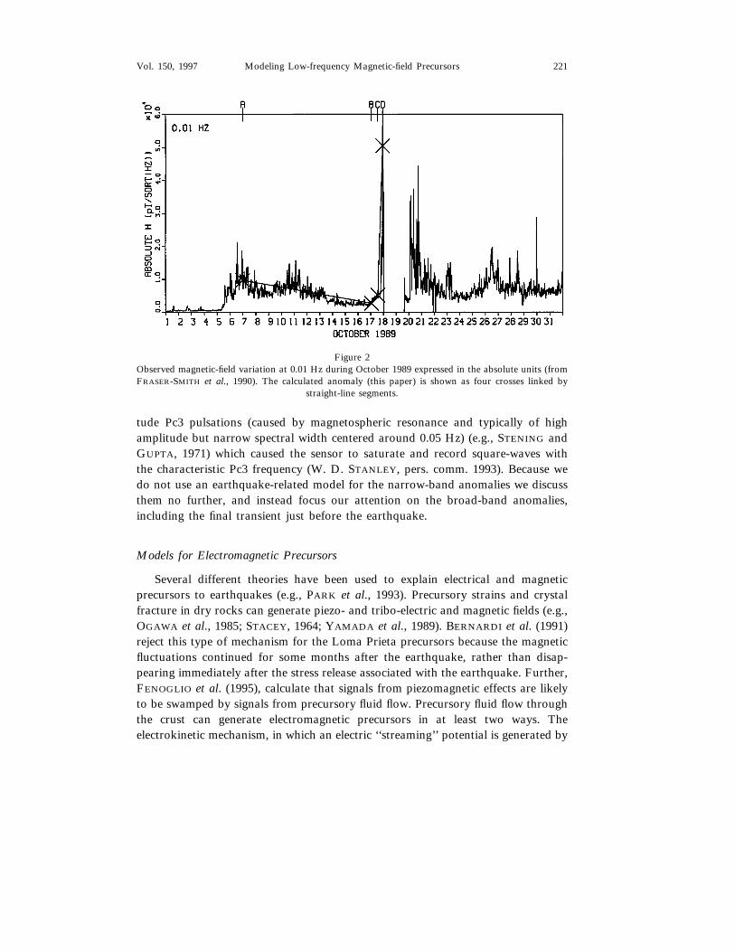
Immediately preceding the Loma Prieta earthquake on 10/18/89, low-frequencymagnetic-noise anomalies were measured on a ULF system about 7 km from theepicenter (FRASER-SMITH et al., 1990; BERNARDI et al., 1991). The magnetic-fielddata (Fig. 1) show that about 3 hours before the earthquake the magnetic field roseto about 100 times the normal background level with the most marked increase inthe 0.01–0.5 Hz range. Figure 2 displays this anomaly at 0.01 Hz in absolute fieldunits. The anomalous behavior started about 9/12/89 with narrow-band fluctua-tions in the 0.05–0.1 Hz and 0.1–0.2 Hz bands (Fig. 1). On 10/5/89 thesenarrow-band signals were replaced by a large and sustained noise increase over allthe frequencies of operation, but strongest at the low frequencies (Figs. 1 and 2).The magnetic activity level then decreased slowly until the day of the earthquake.On that day there was a distinct drop and recovery in background noise in the0.2–0.5 Hz range and finally there was the sharp increase mentioned above. Due toa power failure caused by the main shock, no data were recorded for 39 hoursfollowing the earthquake. When recording resumed, wide-band magnetic fluctua-tions remained high for a few months, though with no obvious correlations toindividual aftershocks which reached up to magnitude 5.4 (BERNARDI et al., 1991;FENOGLIO et al., 1993).

It is necessary to distinguish between the narrow-band anomalies (9/12–10/5/89,visible only in the 0.05 to 0.2 Hz bandwidth) and the broad-band anomalies (10/5to the earthquake on 10/18/89, visible in the entire recorded bandwidth from 0.01to 10 Hz). No published discussion or models (BERNARDI et al., 1991; MERZER,

M. Merzer and S. L. Klemperer220 Pure appl. geophys.,

1990, 1992; DRAGANOV et al., 1991; MERZER and KLEMPERER, 1993; FENOGLIO

et al., 1995) offer any physical explanation for the narrow-band anomalies asearthquake precursors. In contrast, a possible explanation for the narrow-bandanomalies as instrumental noise is that the magnetic storm on 9/19 (most clearlyvisible in the 0.01 to 0.04 Hz and 0.1 to 0.2 Hz bands, Fig. 1) included high-ampli-

Figure 1Magnetic field variations measured during September and October 1989, from FRASER-SMITH et al.(1990). The large gap in the data around 18, 19 October is due to a power failure caused by the LomaPrieta earthquake. The MA index (M) can be converted to an absolute magnetic field amplitude (H) by:

H= (C×2M)1/2 pT/Hz,

where C=constant for each frequency, =2.704×102 at 0.015 Hz decreasing to 7.129×10−3 at 7.5 Hz(FRASER-SMITH et al., 1990). Note that on this log scale an increase of two in measured MA indexcorresponds to a doubling of the absolute field, and an increase of 10 in MA index corresponds to a

30-fold increase in the absolute magnetic field.

Modeling Low-frequency Magnetic-field Precursors 221Vol. 150, 1997

Figure 2Observed magnetic-field variation at 0.01 Hz during October 1989 expressed in the absolute units (fromFRASER-SMITH et al., 1990). The calculated anomaly (this paper) is shown as four crosses linked by

straight-line segments.

tude Pc3 pulsations (caused by magnetospheric resonance and typically of highamplitude but narrow spectral width centered around 0.05 Hz) (e.g., STENING andGUPTA, 1971) which caused the sensor to saturate and record square-waves withthe characteristic Pc3 frequency (W. D. STANLEY, pers. comm. 1993). Because wedo not use an earthquake-related model for the narrow-band anomalies we discussthem no further, and instead focus our attention on the broad-band anomalies,including the final transient just before the earthquake.

Models for Electromagnetic Precursors

Several different theories have been used to explain electrical and magneticprecursors to earthquakes (e.g., PARK et al., 1993). Precursory strains and crystalfracture in dry rocks can generate piezo- and tribo-electric and magnetic fields (e.g.,OGAWA et al., 1985; STACEY, 1964; YAMADA et al., 1989). BERNARDI et al. (1991)reject this type of mechanism for the Loma Prieta precursors because the magneticfluctuations continued for some months after the earthquake, rather than disap-pearing immediately after the stress release associated with the earthquake. Further,FENOGLIO et al. (1995), calculate that signals from piezomagnetic effects are likelyto be swamped by signals from precursory fluid flow. Precursory fluid flow throughthe crust can generate electromagnetic precursors in at least two ways. Theelectrokinetic mechanism, in which an electric ‘‘streaming’’ potential is generated by

M. Merzer and S. L. Klemperer222 Pure appl. geophys.,

subterranean water flow into a dilatant earthquake source region (MIZUTANI et al.,1976), or by episodic flow of high-pressure water in fault zones (BYERLEE, 1993),has been used as the basis of a quantitative model for the Loma Prieta precursors(FENOGLIO et al., 1995), in which a frequency variation of magnetic-field anomaliesto match the observations can be obtained by having an appropriate distributionwith depth of crack lengths in the fault zone. A magnetohydrodynamic model forthe Loma Prieta precursors in which oscillatory flow of conductive fluids coupleswith the earth’s magnetic field has been proposed by DRAGANOV et al. (1991),though a frequency variation of the magnetic-field anomalies to match the observa-tions has not been shown. We find both these electrokinetic and magnetohydrody-namic models (DRAGANOV et al., 1991; FENOGLIO et al., 1995) of questionablecredibility because they are dynamic and require flow of free water in a highlypermeable fault zone, at velocities of 10 cm · s−1 to \1 m · s−1, throughout at leastthe 12-day period of the precursory wide-band magnetic anomalies, in order togenerate the observed anomalies. These fluid flows correspond to pumping c. 1 to1000 km3 of water through the fault zone in the two weeks prior to the earthquake.In contrast, numerical calculations of fluid flux in fault zones yield values ofmm · s−1, not m · s−1 (FORSTER and EVANS, 1991); and models for gravity-drivenregional flow in permeable sedimentary aquifers give long-term flow rates of 10−8

m · s−1 (GARVEN, 1989).In contrast, in this paper we present a quasi-static model, in which the

conductive fault zone acts as an antenna to couple with the external electromag-netic field to generate the observed magnetic anomalies. Precursory changes infault-zone conductivity lead to precursory changes in the observed magnetic field,but we consider no time-dependent effects, i.e. the rapid flow of large volumes offluid forms no part of our model. Previous investigators have calculated thetheoretical change in magnetic field due to conductivity changes at depth (conceptu-ally related to fluid infiltration into a dilatant volume) for specific two-dimensional(RIKITAKE, 1976b), and three-dimensional (HONKURA and KUBO, 1986) models.Although these authors showed that, in principle, observations of short-periodmagnetic variations in the range from a few seconds to a few minutes could be usedto detect conductivity anomalies, their models of deeply buried, broad rectangularconductors only provided enhancements of the magnetic field by up to a factor ofabout two, and no real data were modeled.

The models of RIKITAKE (1976b) and HONKURA and KUBO (1986) are basedon the concept of fluid infiltration into a dilatant volume. This concept fell out offavor with the recognition that significant fluid influx requires significant—andeasily measurable but rarely observed—precursory strains and uplift (HANKS,1974). Nevertheless, it remains appropriate to consider models in which variationsin fault-zone conductivity generate the precursory magnetic-field variations becausechanges in conductivity do not necessarily require fluid influxes (MORRISON et al.,1977; this paper), and because precursory conductivity changes have been reported

Modeling Low-frequency Magnetic-field Precursors 223Vol. 150, 1997

before at least two earthquakes on the San Andreas Fault (MAZZELLA andMORRISON, 1974; PARK, 1991). In this paper we demonstrate how more realisticfault-zone geometries than those used by RIKITAKE (1976b) and HONKURA andKUBO (1986) can cause field enhancements by two orders of magnitude, and can beused to successfully model the observed precursory magnetic-field anomalies over afrequency range of three orders of magnitude. The lack of precursory strain changeto the Loma Prieta earthquake (less than a few nanostrain at 40 km distance:JOHNSTON et al., 1990) is suitable to our hypothesis because we model the requiredconductivity change by changing geometry of existing fluid-filled porosity, ratherthan creation of new porosity.

In following sections of this paper we develop our theoretical model forenhancement of the magnetic-field variations (MERZER, 1990, 1992); we calculateanomalies for a specific geometry of conductors, based on field observations andillustrate that the calculated anomalies match the observed precursors; and wepresent a geologic scenario for the precursory development of the required conduc-tive geometry (MERZER and KLEMPERER, 1993).

Outline of Model

The normal magnetic-noise background is caused by the incidence of externalelectromagnetic waves on the earth’s surface. At the earth’s surface, reflection andtransmission occur, due to the earth’s conductivity. Over the range of frequenciesand conductivities of interest, the reflected magnetic field is practically equal to theincident field; and, as a result, the measured background-level amplitude is twicethat of the incident magnetic field. The implication of this result is that no modelof horizontal conductive layers could create the observed anomalously high mag-netic fields. Even if the conductivity at any depth were to be as high as that ofmetal, no anomalously high magnetic field would be produced.

If this is the case, what configuration can give rise to amplified magnetic fields?In electromagnetic theory, one valid mechanism is an electromagnetic wave imping-ing on a thin infinitely long wire (Fig. 3) with incident electric field Ei parallel to thewire. The field induces a current I within the wire, which acts as an antenna and inturn creates a circumferential magnetic field:

Hc=I

2pr, (1)

where r=distance from the axis of the wire.On the surface of the wire

Hc=I

2pa, (1a)

M. Merzer and S. L. Klemperer224 Pure appl. geophys.,

where a=radius of wire (see Eqs. (9.23) and (9.17) in KAUFMAN and KELLER,1981). If the wire is thin compared to the external wavelength, (1) and (1a) can givethe desired high magnetic fields.

The geophysical implication is that if a highly-conductive long thin region wascreated under or nearly under the magnetometer towards the time of the earth-quake (Fig. 4), then the incident electromagnetic waves would have induced a highcurrent in this region, which in turn created the high magnetic fields.

Our conceptual model is that redistribution of fluids within the fault zone priorto the Loma Prieta earthquake modified the conductivity structure sufficiently tocause the observed magnetic-variation anomalies. The Loma Prieta rupture andmain concentration of aftershocks define a zone dipping 70° to the southwest,extending from about 2 to 18 km depth, and 2 to 3 km wide (U.S. GEOLOGICAL

SURVEY STAFF, 1990). For mathematical simplicity, our analysis models the faultzone as an infinitely long elliptical cylinder with a vertical major axis, which in ourbest-fitting model extends from the surface to the hypocentral depth of 18 km, witha maximum width of 4.5 km. The paper discusses the effect of limiting the cylinderlength to that of the Loma Prieta aftershock zone (70 km), and also aspects ofcylinder impedance computation.

The consideration of precursory conductivity changes is appropriate since directobservations of conductivity increase before earthquakes have been widely re-ported, for example before a series of moderate shocks in the Garm region (former

Figure 3Electromagnetic wave incident on an infinitely long thin wire. The electric field Ei is parallel to the wire.

Hc is the quasi-static magnetic field created around the wire.

Modeling Low-frequency Magnetic-field Precursors 225Vol. 150, 1997

Figure 4Section of highly-conductive region within layered structure of conductivities s1 and s2. The highly-con-ductive region is considered to be a cylinder of elliptic cross section. The magnetic field is calculated (see

text) at the point P on the earth’s surface directly above the ellipse.

U.S.S.R.) (SADOVSKY et al., 1972); before the M=7.8 Tangshan earthquake(QIAN, 1984/85); and before at least two small earthquakes on the San AndreasFault (MAZZELLA and MORRISON, 1974; PARK, 1991). It is appropriate to considerthe conductivity arising particularly in the fault zone because the porosity, perme-ability and fluid content of the fault zone are expected to be different from thesurrounding rocks, based on theoretical modeling (RICE, 1992), laboratory studies(FORSTER and EVANS, 1991), and field observations (WANG, 1984; WANG et al.,1986).

Quantitati6e De6elopment of the Model

Our model is developed in the following stages:i. The basic horizontal layer structure in which the highly-conductive region

occurs.ii. The highly-conductive region itself.

iii. The current created within the region.iv. The magnetic field generated by the current.

M. Merzer and S. L. Klemperer226 Pure appl. geophys.,

(i) Basic Horizontal Layer Structure

Measurements of conductivity made in the Loma Prieta region a few monthsbefore the earthquakes (EBERHART-PHILLIPS et al., 1990a) and again two yearsafter the earthquake (RODRIGUEZ et al., in press) show a complex upper-crustalstructure which becomes less conductive with depth (Fig. 5a). To simplify numericalcalculations we have initially grossly simplified the structure into a two-layer,horizontally layered model (Fig. 5b). The electric and magnetic field distribution(E(z) and H(z)) in the structure can be found by solving Maxwell’s equations (pp.40–44 in KAUFMAN and KELLER, 1981).

(ii) The Highly-conducti6e Body

The highly-conductive body is considered for simplification to be an infinitelylong cylinder of elliptic cross section (Fig. 4) with conductivity sc (the effect ofmaking the length finite is considered in the appendix). It is at depth h and hasvertical and horizontal semi-axes a and b, respectively (b5a). The electric field

Figure 5Magnetotelluric section across the Loma Prieta region (approximately SW–NE). (a) Magnetotelluricmodel (asterisks along top of profile indicate location of MT recording stations) and earthquakehypocenters (heavy cross is main shock, 4 km NW of section, and aftershocks within 5 km of the profileare shown by circles proportional to magnitude) from RODRIGUEZ et al. (in press). Arrow at top ofsection indicates location of FRASER-SMITH et al. magnetometer projected along geologic strike. Notehigh-conductivity tongue under San Andreas. (b) Equivalent conductive model of the horizontal layeringused for computations. (c) Modelling of the high-conductivity tongue under San Andreas [in (a)] as anellipse. This configuration acts as the base for the models in Figure 7. Note that the magnetometer[arrow in (a)] lies immediately above the high-conductivity tongue. Thus the magnetic field values it

records are appropriate to the values computed at point P in Figure 4.

Modeling Low-frequency Magnetic-field Precursors 227Vol. 150, 1997

E(z) computed for the horizontally layered model (Fig. 5b) above is assumed to actalong the length of the cylinder (Fig. 4). Since the field varies with depth, anaverage value (EA6 ) is assumed to excite currents in the body:

EA6=12a

& h+2a

h

E(z) dz. (2)

(iii) Current along Cylinder

If the elliptic section semi-axes a and b are smaller than the wavelength, thecurrent I along the cylinder is

I=EA6 /(zL+zE ), (3)

where zL= internal impedance/unit length, and zE=external impedance/unitlength.

Neglecting the effects of zE (they are discussed in the appendix) we express zL as

zL=Zc /lc, (4)

where Zc=unit surface impedance on the cylinder, and lc=elliptic circumference.lc can be computed from the geometry:

lc=4a · e(m), (5)

where e(m)=complete elliptic integral of the second kind (Ch. 17 in ABRAMOVITZ

and STEGUN, 1965), and m=(1−b2/a2).Zc can be computed by approximating the elliptic cylinder to an infinite plate of

thickness 2b (Fig. 6). The exciting field is simulated by two identical wavestravelling in opposite directions and incident normally on the plate’s surfaces (Fig.6). The ratio of total electric and magnetic fields at the surface gives the requiredimpedance Zc (MERZER, 1990):

Zc=Z0

1+exp[−2gb ]1−exp[−2gb ]

, (6)

where Z0=g/sc, sc= the conductivity of the parallel plate, g= (1+i)/d, d=skindepth= (1/scpfm0)1/2, m0=4p×10−7 henry/m, f= frequency, and i=−1.

(i6) Magnetic Field Generated by Current

External to the elliptic cylinder, the magnetic field H is quasi-static for externalwavelengths considerably larger than a and b. In such conditions, the fields can beexpressed as a potential obeying Laplace’s equation and calculated (MERZER, 1990)using a conformal transformation (SPIEGEL, 1964) of the known field external to acircular cylinder. Assuming that the field H is circumferential to the ellipsoid and

M. Merzer and S. L. Klemperer228 Pure appl. geophys.,

Figure 6Approximation of elliptic section to parallel plate.

does not cut the perimeter, its value at point P on the surface above the ellipse(Fig. 4) is (assuming uniform unit relative permittivity in the whole region):

HP=I

2p(h2+b2+2ah)−1/2. (7)

Comparison of HP with the ambient magnetic field at the surface (H(z=0))gives the relative increase in magnetic field due to the presence of the highly-con-ductive region. HP, the maximum value of the magnetic field, decreases awayfrom the top of the ellipse. For the special case in which h=0 (ellipse reachesthe surface) the field is initially inversely proportional to the distance from thecenter of curvature at the tip of the ellipse to the point of measurement(MERZER, 1990).

Modeling Low-frequency Magnetic-field Precursors 229Vol. 150, 1997

Comparison of Computations on Model to Obser6ations

Using the theoretical result of the previous section, a model (Fig. 8) has beenbuilt to simulate the magnetometer field measurements at four points in time: A, B,C and D in the field measurements (Figs. 2, 7, 8). A is on 10/7 UT after the initialrise, B is at the start of 10/17 UT, C is halfway through 10/17 UT, and D is thelarge peak immediately preceding the earthquake on 10/18 UT.

At each stage, different elliptic cylinders of uniform, high conductivity

Figure 7Highly-conductive elliptic cylinder superimposed on horizontal layer structure of Figure 5b. All cylindershave the same conductivity 5 S · m−1. Indicated lengths are in kilometers (except for 20 m depth of A,

which is not to scale). Models A, B, C and D correspond to the points in Figure 8a.

M. Merzer and S. L. Klemperer230 Pure appl. geophys.,

Figure 8a

sc=5 S · m−1

are superimposed onto the horizontal layer structure of Figure 5b. Using equation(7), the anomalous magnetic field HP is computed immediately above the conduc-tive cylinder. The ratio (RH ) of the anomalous magnetic field (HP ) to the ambientmagnetic field at the earth’s surface [H(z=0)] is calculated and expressed as a jump(DM) in the MA index (FRASER-SMITH et al., 1990);

DM=2 log2(RH ). (8)

The values of HP are plotted (Fig. 8a) relative to base values which we calculate asthe average of the magnetic indices M (Fig. 1) during the quiet period from 1–10September 1989 (Fig. 8b). We interpret these base values as the background due tothe horizontal layer structure of Fig. 5b. Good fits are obtained over most of the

Modeling Low-frequency Magnetic-field Precursors 231Vol. 150, 1997

range of frequencies, and the ratios between the computed results and observeddata are shown in Figure 9. Note that obtaining the base values by averaging themagnetic indices M, corresponds to taking a geometric average of the power of themagnetic field H2 (Fig. 1). Had we used an arithmetic average of H2, the basevalues would be higher, implying that the precursory signals are less anomalous(i.e., relatively easier to explain) and fits analogous to those of Figure 9 would beobtained with sc=3.3 S · m−1 rather than sc=5 S · m−1. However, their highervalues appear to be due to H2 being more sensitive than M to anomalous amplitudebursts from the quiet ambient background. Because of this greater sensitivity whichcan create spurious averages, we decided to use the M averages as base values.

Figure 8(a) Computational results superimposed on magnetic field amplitudes of Figure 1 for October 1989. 4points: A, B, C and D are examined corresponding to the models in Figure 7. x is computed points withconnecting straight lines. (b) Figure 1 for September 1989 showing the base lines, which are the average

ambient field values during the first 10 days of this month. These base lines are shown also in (a)

M. Merzer and S. L. Klemperer232 Pure appl. geophys.,

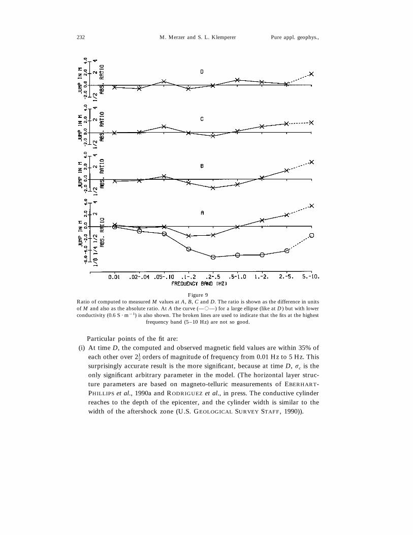
Figure 9Ratio of computed to measured M values at A, B, C and D. The ratio is shown as the difference in unitsof M and also as the absolute ratio. At A the curve (—�—) for a large ellipse (like at D) but with lowerconductivity (0.6 S · m−1) is also shown. The broken lines are used to indicate that the fits at the highest

frequency band (5–10 Hz) are not so good.

Particular points of the fit are:(i) At time D, the computed and observed magnetic field values are within 35% of

each other over 212 orders of magnitude of frequency from 0.01 Hz to 5 Hz. This

surprisingly accurate result is the more significant, because at time D, sc is theonly significant arbitrary parameter in the model. (The horizontal layer struc-ture parameters are based on magneto-telluric measurements of EBERHART-PHILLIPS et al., 1990a and RODRIGUEZ et al., in press. The conductive cylinderreaches to the depth of the epicenter, and the cylinder width is similar to thewidth of the aftershock zone (U.S. GEOLOGICAL SURVEY STAFF, 1990)).

Modeling Low-frequency Magnetic-field Precursors 233Vol. 150, 1997

(ii) Between B and C, the observed field dips at higher frequencies but at lowerfrequencies it increases monotonically. The computed field values show thisdetailed behavior.In the highest frequency band (5–10 Hz) the fits are not so good. This may

occur because the approximation of ellipse section dimensions being less than theincident wavelength becomes less valid at these higher frequencies (MERZER, 1990).

The elliptic sections of A, B, C and D (Fig. 7) were not obtained by strictinversion. Instead their size and depth were obtained using qualitative guidelinesbased on the variation of the anomalous magnetic field (HP ) with frequency:

(i) At time A, HP is more or less uniform in frequency. This can be ascribed to ashallow cylinder near the surface, which can contribute to HP over a widerange of frequencies.

(ii) Between times B and C, HP dips at higher frequencies, although at lowerfrequencies it increases. This can be ascribed to the cylinder at C being largerand deeper than at B. Making the cylinder larger at C increases HP at allfrequencies, however making it deeper attenuates the field at the higherfrequencies only, and more than offsets the increase at these frequencies due toC being larger.

(iii) At time D, the larger jump in HP is only significant at lower frequencies. Thiscan be ascribed to a large conducting cylinder stretching from the surface to alarge depth. At low frequencies the whole cylinder contributes to HP ; while athigher frequencies only the upper part can contribute, since the horizontalconductive layering (Fig. 5b) attenuates any penetration to lower depths.

We have experimented with models in which the conductivity varies with timewhile the size of the conductive zone remains constant. In Figure 9 we compareresults at time A for a model with the conductive ellipse the same size as in D (Fig.7) but with conductivity reduced by a factor of 8 to 0.6 S · m−1. This lowerconductivity matches the observed field variations at low frequencies, but cannotmatch the decrease in magnetic field with increasing frequency, because too muchof the conductive ellipse is deeper than the skin depth for high frequencies. Only amodel of the type in Figure 7, with temporal variation in the size of the conductivezone, seems to fit the behavior of the magnetic-field amplitudes at A, B, C and Dwith their varying dependence in frequency.

The above comparisons were carried out for an infinitely long cylinder, when inorder to be compatible with reality its length should be approximately that of theLoma Prieta fault zone (70 km as defined by the extent of the aftershocks, U.S.GEOLOGICAL SURVEY STAFF, 1990). Consideration of input impedances in buriedbare antennas (KING and SMITH, 1981) indicates that full excitation is essentiallyachieved when antenna length is of the order of a half-wavelength for thesurrounding medium. For an upper-crustal conductivity of 0.033 S · m−1 as used inthis paper, this half-wavelength is 90 km, which is comparable to the above faultzone length. Although further accurate calculations are needed, the above compari-

M. Merzer and S. L. Klemperer234 Pure appl. geophys.,

sons suggest that the finite-length of the fault zone should not alter our resultssubstantially.

The influence of the external impedance zE, which was not included in Equation(3), can be quite substantial (see appendix). However these effects, even though theycause distortions in the above comparisons, do not alter our fundamental result: aconductive cylinder at depth can produce substantial increases in the magnetic fieldsuch as observed prior to the Loma Prieta earthquake.

Having presented the electromagnetic aspects of generation of large magnetic-field due to high conductivity preceding the Loma Prieta earthquake, in thefollowing section we discuss possible causes for the high conductivity and suggest aphysical and geologic model consistent with our mathematical model.

De6elopment of Conducti6ity in Fault Zone

Our best model fits were obtained assuming a bulk conductivity sc=5 S · m−1

for the entire fault zone. In this section wei. discuss the need for such a high conductivity, and

ii. suggest a model for it.

The Need for High Conducti6ity to Fit the Obser6ed Magnetic-field Variations

If the elliptic conductor is assumed to extend down to the epicentral depth of 18km as in Figure 7, then 5 S · m−1 is the lowest conductivity value that gives theobserved high magnetic fields at time D immediately before the earthquake.

If the elliptic section has a greater depth, then the value of sc can be reduced.However, there appears to be no reason to give the conductor a greater depth, sincethe 3D velocity and magnetotelluric models for the region (EBERHART-PHILLIPS etal., 1990a,b; RODRIGUEZ et al., in press; and Fig. 5a) do not indicate anomalousbehavior below the epicentral depth, and significantly deeper aftershocks were notrecorded.

In the other stages (A, B, C in Fig. 7) the elliptic sections were given the sameconductivity value of sc=5 S · m−1 because modeling results show that sc cannotbe reduced substantially while still matching the dependence of magnetic-fieldvariation on frequency (Fig. 9).

Prerequisites for the High-conducti6ity Model

In order to build such a model three factors require consideration:i. The conductivity of crustal fluids.

ii. Porosity of the San Andreas Fault zone.iii. Measured conductivity of the Loma Prieta Fault zone.

Modeling Low-frequency Magnetic-field Precursors 235Vol. 150, 1997

Conducti6ity of crustal fluidsConductivity is controlled by two principal factors, a. salt concentration and b.

temperature and pressure conditions.a. Salt concentration. Seawater contains approximately 0.5 M NaCl, where M

denotes molality, or concentration in moles per kg of solvent, a quantity invariantwith pressure and temperature. The salt concentration in metamorphic inclusionfluids ‘‘is normally less than 50 and usually about 10 wt.%’’ (equivalent to 17 to 2M) (FYFE et al., 1978). Thermal and mineral springs in the California Coast rangeshave concentrations up to 0.4 M but are typically shallow systems dominated bymeteoric water (WHITE et al., 1973). Studies of groundwater in deep mines haveshown a general increase in salinity with depth, in the Canadian Shield from below0.1 M above 500 m to over 2.5 M at 1500 m depth (FRAPE and FRITZ, 1987). Wetherefore take the likely range of salinity of waters in the Loma Prieta Fault zoneto be 0.5 M to 2.5 M.

b. Temperature and pressure conditions. QUIST and MARSHALL (1968) mea-sured electrical conductance of 0.001 to 0.01 M NaCl solutions, and HWANG et al.(1970) the conductance of 0.1 to 3 M KCl solutions at temperatures of 0 to 500°Cand pressures of 0.001 to 3 kb (Fig. 10). Mean heat flow around the San AndreasFault zone in northern California is 83 mW · m−2 (LACHENBRUCH and MCGARR,1990), implying that temperatures of 300°C may be reached at depths as shallow as10 km (LACHENBRUCH and SASS, 1977). For temperatures below 300°C andpressures above 50 MPa, brine conductivity is essentially isobaric (QUIST andMARSHALL, 1968).

Based on a salinity of up to 2.5 M and temperatures rising to 300°C, fluidconductivity may be as high as 100 S · m−1 (Fig. 10), and probably averages no lessthan 25 S · m−1 over the entire brittle fault zone.

Porosity of the San Andreas Fault zoneDirect observations in a 600-m deep well close to the San Andreas Fault at

Stone Canyon suggest macrocrack porosities of 5 to 10% (STIERMAN and KOVACH,1979). Detailed gravity modeling across the San Andreas Fault near Bear Valley,coincident with a reflection profile, implies a density contrast of at least 200kg · m−3, and hence porosities of at least 12%, across a zone 2 to 3 km wide andabout 15 km deep (STIERMAN, 1984). These observations suggest that substantialporosities exist in the creeping zone of the San Andreas Fault, despite theexpectation that ductile creep between earthquakes leads to compaction andporosity reduction (SLEEP and BLANPIED, 1992). Although low-velocity zones (andhence highly porous zones) may be less well-developed on locked parts of the SanAndreas Fault (MOONEY and GINZBURG, 1986), STIERMAN (1984) modeled gravityacross a locked part of the fault with a density reduction of 50 to 100 kg · m−3

(porosity of c. 3 to 6%) across a c. 5-km-wide zone to 10 km depth, and a densityreduction of 400 km · m−3 (porosity of c. 25%) across a 200-m-wide zone at thefault trace. Apparently, porosities of 10% and locally 20%, are not out of the

M. Merzer and S. L. Klemperer236 Pure appl. geophys.,

question within the Loma Prieta fault zone 2 to 3 km wide and extending to 18 kmdepth.

Such porosities can only exist at depth if filled with fluids at near-lithostaticpressure. However, measurements in oil wells show a zone of near-lithostatic fluid

Figure 10Straight-line fits to experimentally determined conductivity of NaCl solutions (QUIST and MARSHALL,1968) and KCl solutions (HWANG et al., 1970) at different molality, temperature and pressure. For thelikely molality and temperature range of crustal fluids in the Loma Prieta fault zone, 0.5 to 2.5 M, and

100 to 300°C, the likely range of conductivities is 25 to 100 S · m−1.

Modeling Low-frequency Magnetic-field Precursors 237Vol. 150, 1997

pressure in the California Coast ranges east of the San Andreas Fault (BERRY,1973), particularly in the Franciscan rocks such as crop out east of the Loma Prietafault zone, and from which fluids may be channeled into the relatively permeablefault zone (IRWIN and BARNES, 1975). An important source of brines into theLoma Prieta fault zone may be the Pliocene-Recent underthrusting of oceanic crustbeneath the Loma Prieta hypocentral region (PAGE and BROCHER, 1993). The 3.5Ma elapsed since underthrusting began is small compared to the c. 100 Ma requiredto dehydrate the seismic upper crust (BAILEY, 1990). Observation of small precur-sory water-level changes in a well in the San Andreas Fault zone (KOVACH et al.,1975) and order-of-magnitude changes in stream flow possibly before the LomaPrieta earthquake (ROELOFFS, 1993) and certainly immediately after the earth-quake (ROJSTACZER and WOLF, 1992), further imply that hydrologic and earth-quake processes are closely linked in this area. Finally, evidence of near-frictionlessfaulting during the Loma Prieta earthquake indicates the existence of near-litho-static pore pressure at the time of rupture (ZOBACK and BEROZA, 1993).

Measured conducti6ity of the Loma Prieta fault zoneRODRIGUEZ et al. (in press) have modeled the deep geoelectric structure of the

Loma Prieta epicentral region, using magnetotelluric data acquired 5 monthsbefore, 7 months after, and 30 months after the Loma Prieta earthquake. Accept-able earth models require ‘‘low-resistivity bodies of about 3 ohm-m [0.33 S · m−1]in the 4–19 km depth range near the San Andreas Fault, with the dip, shape andprecise distribution not resolvable’’ but conductivities of only 0.001 S · m−1 outsidethe fault zone and below 4 to 7 km depth (RODRIGUEZ et al., loc. cit.). Theirbest-fit model, which shows the highly conductive tongue of material essentiallycoincident with projected locations of Loma Prieta aftershocks, and with a width of4–7 km, is shown in Figure 5a. This result has only ‘‘minor differences’’ (RO-

DRIGUEZ et al., loc. cit.) from the model based only on data acquired before theLoma Prieta earthquake (EBERHART-PHILLIPS et al., 1990a,b). RODRIGUEZ et al.consider possible causes for the high conductivity of the fault zone and concludethat unless serpentinite is ubiquitous in the fault zone—unlikely because of itsabsence in local outcrop—‘‘resistivities in these deep rocks must mostly be due tofracturing and fluid content’’.

This high fault-zone conductivity is apparently not anomalous: PHILLIPS andKUCKES (1983) found 0.1 S · m−1 conductivity within a creeping section of the SanAndreas Fault near Hollister; and laboratory measurements of saturated gougefrom the San Andreas Fault show conductivities of 0.02 to 0.2 S · m−1 at confiningpressures of 20 to 200 MPa (LOCKNER and BYERLEE, 1985; WANG, 1984).

The Model

Conductivity of porous sedimentary and crustal rocks is most commonlyestimated from the empirical Archie’s law (e.g., HERMANCE, 1979):

M. Merzer and S. L. Klemperer238 Pure appl. geophys.,

sc=sffn (sf : fluid conductivity; f : porosity; n : empirical exponent).

For most rocks, an excellent fit to laboratory data is obtained for n=2 (BRACE

et al., 1965). A fault-zone conductivity of 0.33 S · m−1 prior to the earthquake(RODRIGUEZ et al., in press) implies a porosity of 7 to 11%—values within thebounds discussed—for the appropriate fluid conductivity of 25 to 75 S · m−1 (seeabove). A fifteen-fold increase in fault zone conductivity to 5 S · m−1 immediatelyprior to the earthquake, as implied by our theoretical model for the observedmagnetic-field anomalies, accordingly requires either

i. a large influx of water to increase the porosity to 25 to 45%; orii. an increase in fluid conductivity by a factor of 15; or

iii. a change in the Archie’s-law exponent from n=2 to n=1.The lack of significant strain precursors to the Loma Prieta earthquake (less

than a few nanostrain at sites 40 km distant; or less than the strain due to slip ina M=5.3 earthquake, JOHNSTON et al., 1990) makes impossible the creation ofnew porosity within the fault zone on the scale required (possibility i.). It isessentially impossible to increase the fluid conductivity by an order of magnitude(possibility ii.), since this would require increasing the fluid temperature by severalhundred Kelvin or by increasing the salinity by more than an order of magnitude(Fig. 10). In the geochemical precursors to the 1/17/95 M=7.2 Kobe, Japan,earthquake, salinity increased by ‘‘only’’ about 50% (TSUNOGAI and WAKITA,1995).

We therefore consider possibility iii: A precursory change in the fault-zonestructure resulting in a change in the effective exponent in Archie’s Law (MOR-

RISON et al., 1977). For fluid conductivity of 100 S · m−1 and fault-zone porosity of7%, changing the Archie’s Law exponent from n=2 to n=1 results in an increasein fault-zone conductivity from the 0.33 S · m−1, observed months prior to theLoma Prieta earthquake, to 5 S · m−1, immediately prior to the earthquake.

Archie’s Law has been regarded as an empirical expression of the statisticaldistribution of connected vs. unconnected pores containing conductive fluid in ahighly resistive matrix (HERMANCE, 1979). If the distribution of porositychanges—particularly (Fig. 11) between low-aspect-ratio porosity (spheroidal inclu-sions) and high-aspect-ratio porosity (planar cracks)—then deviations from anArchie’s Law exponent of n=2 are to be expected. It is this behavior that seems tobe responsible for the laboratory observations of drops in resistivity in saturatedrocks immediately prior to fracture (BRACE and ORANGE, 1968). BRACE andORANGE (pp. 1442–1443) state that: ‘‘An exponent of n=1 is in one senseconsistent with our current view of crack development during dilatancy of crys-talline rocks. New cracks are probably strongly oriented parallel with the axis ofmaximum compression. Electrically, then, new conducting paths can be approxi-mated as parallel tubes or slits. One might expect their contribution, the new crackconductivity, to vary linearly with crack porosity giving an exponent n=1. ’’

Modeling Low-frequency Magnetic-field Precursors 239Vol. 150, 1997

Figure 11Conceptual cartoon to illustrate how modifying the geometry of a constant-volume porosity candramatically alter the fault-zone conductivity. a. Normal situation: 7% 2 M brine in pores, Archie’s Lawn=2, and s=0.33 S · m−1. b. Preceding earthquake: 7% 2 M brine now in cracks, Archie’s Law n=1,and s=5.0 S · m−1. The cartoon shows modification along the fault in the horizontal plane but in

addition it can also occur in the vertical plane.

Electron microscopy has been used in subsequent studies to document the increas-ing number of microcracks forming with increasing aspect ratios in the range of 102

to 104 (KRANZ, 1979), and ultimately the coalescence of these microcracks to formopen fractures (WONG and BIEGEL, 1985), as compressional tests proceed towardsfailure. The pioneering experiments of BRACE and ORANGE (1968) showed order-of-magnitude drops in resistivity prior to the fracturing of previously unfracturedrock, and subsequent experiments have shown that drops in resistivity, albeitsmaller, also occur during stick-slip sliding on a pre-cut surface (WANG et al.,1978).

Based on these laboratory experiments, in principle large changes in conductiv-ity could take place (Fig. 11) by connecting isolated pores to form interconnectingor highly overlapping planar cracks (MERZER and KLEMPERER, 1992), by redis-tributing existing porosity with essentially no change in total pore volume (corre-sponding to the lack of an observable strain precursor, JOHNSTON et al., 1990) andessentially no formation of new crack surfaces (obviating the need for precursorywork to form such cracks). In practice some increase in porosity (precursorydilatancy) probably occurs, and hence fracture surfaces probably form, before themain earthquake rupture (BRACE et al., 1966).

M. Merzer and S. L. Klemperer240 Pure appl. geophys.,

Discussion

We have shown that a precursory increase in fault-zone conductivity couldcause the anomalous magnetic-field variations that were observed before the LomaPrieta earthquake. We have demonstrated that, for values of fault-zone porosityand fluid conductivity within the bounds of those estimated by other techniques, aredistribution of existing porosity can provide the required increase in conductivity.A fault-zone with 7% porosity filled with brine of conductivity 75 S · m−1 has aconductivity of 5 S · m−1 for Archie’s Law exponent of n=1 but only 0.33 S · m−1

for n=2. Though this fluid conductivity and this fault-zone porosity are both at thehigh end of the ranges commonly considered, it is important to note that thesevalues are not determined by our model. Rather, the RODRIGUEZ et al. (in press)and the EBERHART-PHILLIPS (1990a,b) magnetotelluric results require fluid conduc-tivity and porosity in the range 75 S · m−1/7% to 25 S · m−1/11%. If we assumelower conductivity (sub-sea-water salinity or lower temperatures) then Rodriguez’magnetotelluric results imply yet more extreme porosity values to depths\15 km.Our model requires the complete change from Archie’s Law n=2 behavior to n=1behavior of different parts of the Loma Prieta Fault zone at different times up to12 days before the earthquake (times A, B, C and D, Fig. 8). Though thisrequirement is severe, there is no need to force many km3 of water through the faultzone, as is needed to interpret the precursory anomalies purely in terms of theelectrokinetic (MIZUTANI et al., 1976) and magnetohydrodynamic (DRAGANOV etal., 1991) models discussed in the Introduction to this paper.

In addition, our model can be used to explain the continuation of high magneticfields for months after Loma Prieta (FENOGLIO et al., 1993). The high magneticfield can be ascribed to the fault zone continuing to exhibit n=1 behavior with theresultant high conductivity, and only gradually returning to n=2 behavior withlower conductivities. Support for this supposition comes from shear-strain measure-ments at San Juan Batista (GWYTHER et al., 1992), which showed that, for monthsfollowing the earthquake, shear-strain (g1) along the fault direction remainedrelatively constant. Such constancy would imply that the fault zone structureremained static during this period i.e., within the n=1 configuration associatedwith the earthquake.

Though our model requires the presence, and other published models themovement, of large volumes of conductive fluid, it is intriguing to speculate whetherother conductivity mechanisms might exist. Other common conductive phases inthe crust are graphite and some metal sulphides and oxides (including the magnetitepresent in serpentinite) (e.g., JONES, 1992). Some unsaturated graphite granulitesshow an increase in conductivity by up to a factor of three as confining pressure isincreased from 20 to 200 MPa (GLOVER and VINE, 1992), due to increasingconnectivity of the graphite phase. However, the pressures required to achieve thissmall conductivity increase are considerably greater than the permissible deviatoric

Modeling Low-frequency Magnetic-field Precursors 241Vol. 150, 1997

stress in the San Andreas Fault zone (LACHENBRUCH and MCGARR, 1990); theeffect is reversed if the graphitic granulites are saturated (GLOVER and VINE, 1992);and we know of no evidence for enhanced graphite (or metal sulphide or oxide)concentrations in the San Andreas Fault zone.

In our modeling of the Loma-Prieta earthquake we have neglected the elektroki-netic effect (MIZUTANI et al., 1976) and the magnetohydrodynamic effect(DRAGANOV et al., 1991). However, in other earthquakes these effects may be moresignificant and they must all (including the dilatant conductive effect of this paperand perhaps, piezo- and tribo-electric effects, YAMADA et al., 1989) act togethersimultaneously. Because these many different effects are occurring simultaneously,we might expect that the precursory signatures of different earthquakes will be veryvariable, depending on many essentially local conditions of rock type, fluid contentand character. Our model seems to imply that anomalies recorded before futureearthquakes will have very different characters and amplitudes, perhaps not relatedin any simple way to the magnitude and precise location of the impendingearthquake, just as conductivity variations precursory to rockbursts in mines haveexceedingly variable character (STOPINSKI and TEISSEYRE, 1982), and precursorychanges in fault-zone conductivity have been absent for at least two small SanAndreas earthquakes (BUFE et al., 1973; MORRISON et al., 1979) but present for atleast two others (MAZZELLA and MORRISON, 1974; PARK, 1991). Although addi-tional ULF sensors have now been installed along the San Andreas Fault (TEAGUE

et al., 1994), the observations of additional precursory magnetic-field variationsbefore San Andreas earthquakes will neither prove nor refute our hypothesis unlessadditional measurements, e.g., of fault-zone conductivity and spatial variation ofULF fields, are made simultaneously.

Conclusions

Our dilatant-conductive model closely predicts the ULF magnetic-field anoma-lies observed over a 12-day period before the Loma Prieta earthquake. In particu-lar, at the peak anomaly three hours before the earthquake, there is a maximumdeviation of only 35% between predicted and measured results over a frequencyrange from 0.01 to 5 Hz, even though only one truly arbitrary parameter (fault-zone conductivity) is used in the model. All other parameters derive from indepen-dent data on the Loma Prieta earthquake and epicentral region.

Our dilatant-conductive model requires further investigation of both geologicaland electromagnetic aspects. The geological aspect of concern is the requirement forhigh fracture connectivity. Electromagnetic induction effects within the zone andthe finite length of the highly conductive zone are both discussed in this paper (theformer in the appendix); and other electromagnetic aspects, such as wavelengthvis-a-vis dimensions of the elliptic section, have been discussed elsewhere (MERZER,

M. Merzer and S. L. Klemperer242 Pure appl. geophys.,

1990). Further investigation may be necessary regarding initial perturbatory effectsdue to the observed 0.33 S · m−1 tongue (RODRIGUEZ et al., in press). Neither ourdilatant-conductive model, nor any other published model, has suggested anyearthquake-precursor explanation for the narrow-band, 0.1 Hz anomalies observedfrom one month to two weeks before the earthquake. However, these issues shouldnot dissuade consideration of our model, as it is the only quantitative model yetavailable to explain both the magnitude and frequency of the observed wide-bandanomalies, and because it provides good fits for data during the final two weeksbefore the earthquake over the entire measured frequency range.

The close fit between theory and observation indicates that the ULF observa-tions may not be coincidental, but could be a precursory phenomenon with a soundgeophysical basis. Such a sound geophysical basis associated with careful modelingcould make ULF observations more understandable, and would enable them to bemore reliably used to predict oncoming earthquakes.

Acknowledgments

We thank Tony Fraser-Smith for many helpful discussions, and thank him andMark Fenoglio for providing the original magnetic-field data. We thank BrianRodriguez for providing his MT model for the Loma Prieta region prior topublication, and Bruce Nesbitt and George Parks for discussions pertaining to theconductivity of aqueous solutions. Dal Stanley and Frank Morrison wrote detailedreviews, and Jim Wait provided welcome encouragement. MM thanks his col-leagues at RAFAEL and also at the Technion and the Geophysical Institute for themany helpful discussions in the development of this work. SLK received partialsupport for this work from NSF grant EAR-9117834.

Appendix: External Impedance Effects

In our electromagnetic analysis we took the relation between the exciting fieldEA6 and the current (I) created in the elliptic cylinder to be:

I=EA6 /(zL+zE ) (3)

where zL= internal impedance/unit length, and zE=external impedance/unitlength.

In the main body of the paper only the internal impedance zL was used in thecomputations. Here we make an estimate for the influence of the externalimpedance zE. Two examples are considered—points A and D (Fig. 2), at which thelargest anomalies occur.

In both of these examples:

Modeling Low-frequency Magnetic-field Precursors 243Vol. 150, 1997

i. Circular cylinders are considered for simplicity with radii (c0) equal to theaverage of the semi-major and semi-minor axes of the respective ellipticcylinders. Such circular cylinders are equivalent to their respective ellipticcylinders for computing impedances (ELLIOT, 1981).

ii. The frequency considered is 0.01 Hz, at which the largest anomaly occurs.iii. The ratio RZ of the internal impedance to the total impedance:

RZ=�zL �

�zL+zE � (A.1)

is computed. It gives the relative reduction of the current generated due toexternal impedance effects.For circular cylinders the internal impedance for a vertically-incident plane

wave (eq. (3) in WAIT, 1978) is:

zL=1

2pc0

(imwv/sw )1/2 I0(ikwc0)I1(ikwc0)

, (A.2)

where c0=cylinder radius, mw=magnetic permeability of cylinder (free spacevalue), sw=conductivity of cylinder=5 S · m−1, v=radial frequency, k2

w=−imwv(sw+iowv):imwvsw, ow=relative permittivity of cylinder=10, I0, I1=modified Bessel functions, i=−1.

Their external impedance ZE is (eq. (13) in WAIT, 1978):

zE=−(im0v/2p)[ln(0.89kc0)+ip/2−T(a)], (A.3)

where m0=magnetic permeability in ground (free space value), k2=−im0v(s+iov):−im0vs, s=conductivity of ground, o=relative permittivity of ground=10, a=2ikh, h=depth of cylinder, T(a)�0.5 for small depths h (such that a�1as in our case).

Using the above equations we consider points A and D.

Anomaly A

The average radius (c0) is 1100 m (see Fig. 8). The cylinder is totally embeddedin a medium of conductivity

s=0.033 S · m−1.

Substitution in Equations (A.2) and (A.3) above gives a reduction RZ (eq. (A.1)) ingenerated current

RZ=0.67

i.e., the current, and therefore the magnetic field, is reduced by about one-third,which is about the deviation between the computed and experimental results (Fig.9).

M. Merzer and S. L. Klemperer244 Pure appl. geophys.,

Thus in this example external impedance effects do not substantially changeresults.

Anomaly D

Here the average radius (c0) is 5625 m. The ellipse (Fig. 8) is embedded in twolayers of conductivity 0.001 S · m−1 and 0.033 S · m−1. Substitution of eachconductivity in equations (A.2) and (A.3) above gives a reduction (RZ ) in generatedcurrent:

RZ=0.09 and 0.13 respectively.

This is a substantial reduction in current. However:1. The resultant generated field is still substantially above the normal ambient field

(about 10 times) i.e., the essential phenomenon exists and is not obliterated.2. The large observed field can be obtained using an ellipse some 7 to 11 times

thinner than in Figure 8 i.e., about 0.5 km width. This width, though less thanthat of the Loma Prieta aftershock zone, is perhaps more comparable with theexpected width of intense shearing and high porosity in the fault zone (cf.STIERMAN, 1984).

Conclusions

Even though external impedance effects cause distortions, the simple modelpresented in the paper remains relatively correct. For ellipse A their effect isrelatively minor. For ellipse D their effect is more substantive. However thephenomenon of a large jump in magnetic field remains, and the observed jump canbe obtained using thinner but still geologically realistic elliptic cylinders.

REFERENCES

ABRAMOWITZ, M., and STEGUN, I. A., Handbook of Mathematical Functions (Dover Publications, Inc.,New York, 1965).

BAILEY, R. C. (1990), Trapping of Aqueous Fluids in the Deep Crust, Geophys. Res. Letts. 17,1129–1132.

BERNARDI, A., FRASER-SMITH, A. C., MCGILL, P. R., and VILLARD, JR., O. G. (1991), ULF MagneticField Measurements near the Epicenter of the Ms 7.1 Loma Prieta Earthquake, Phys. Earth and Plan.Int. 68, 45–63.

BERNARDI, A., FRASER-SMITH, A. C., and VILLARD, JR., O. G. (1989), Measurement of BARTMagnetic Fields with an Automatic Geomagnetic Pulsation Index Generator, I.E.E.E. Trans. Electro-magn. Comp. 31, 413–417.

BERRY, F. A. F. (1973), High Fluid Potentials in California Coast Ranges and their Tectonic Significance,Am. Assoc. Petrol. Geol. Bull. 57, 1219–1249.

Modeling Low-frequency Magnetic-field Precursors 245Vol. 150, 1997

BRACE, W. F., and ORANGE, A. S. (1968), Electrical Resisti6ity Changes in Saturated Rocks duringFracture and Frictional Sliding, J. Geophys. Res. 73, 1433–1445.

BRACE, W. F., ORANGE, A. S., and MADDEN, T. R. (1965), The Effect of Pressure on the ElectricalResisti6ity of Water-saturated Crystalline Rocks, J. Geophys. Res. 70, 5669–5678.

BRACE, W. F., PAULDING, JR., B. W., and SCHOLZ, C. (1966), Dilatancy in the Fracture of CrystallineRocks, J. Geophys. Res. 71, 3939–3953.

BUFE, C. G., BAKUN, W. F., and TOCHER, D., (1973), Geophysical Studies in the San Andreas FaultZone at the Stone Canyon Obser6atory, California, Stanford University Publications in GeologicalSciences 13, 86–93.

BYERLEE, J. (1993), Model for Episodic Flow of High-pressure Water in Fault Zones before Earthquakes,Geology 21, 303–306.

DRAGANOV, A. B., INAN, U.S., and TARANENKO, Y. N. (1991), ULF Magnetic Signatures at the EarthSurface due to Ground Water Flow: A Possible Precursor to Earthquakes, Geophys. Res. Lett. 18,1127–1130.

EBERHART-PHILLIPS, D., LABSON, V. F., STANLEY, W. D., MICHAEL, A. J., and RODRIGUEZ, B. D.(1990a), Preliminary Velocity and Resisti6ity Models of the Loma Prieta Earthquake Region, Geophys.Res. Lett. 17, 1235–1238.

EBERHART-PHILLIPS, D., LABSON, V. F., STANLEY, W. D., MICHAEL, A. J., and RODRIGUEZ, B.(1990b), Preliminary Velocity and Resisti6ity Models of the Loma Prieta Earthquake Region, Unpub-lished MS, 14 pp.

ELLIOT, R. S., Antenna Theory and Design (Prentice-Hall, Inc., New Jersey 1981).FENOGLIO, M. A., FRASER-SMITH, A. C., BEROZA, G. C., and JOHNSTON, M. J. S. (1993), Comparison

of Ultra-low Frequency Electromagnetic Signals with Aftershock Acti6ity during the 1989 Loma PrietaEarthquake Aftershock Sequence, Bull. Seismol. Soc. Am. 83, 347–357.

FENOGLIO, M. A., JOHNSTON, M. J. S., and BYERLEE, J. D. (1995), Magnetic and Electric FieldsAssociated with Changes in High Pore Pressure in Fault Zones; Application to the Loma Prieta ULFEmissions, J. Geophys. Res. 100, 12951–12958.

FORSTER, C. B., and EVANS, J. P. (1991), Hydrogeology of Thrust Faults and Crystalline Thrust Sheets:Results of Combined Field and Modeling Studies, Geophys. Res. Lett. 18, 979–982.

FRAPE, S. K., and FRITZ, P., Geochemical trends for groundwaters from the Canadian Shield. In SalineWater and Gases in Crystalline Rocks (eds. Fritz, P., and Frape, S. K.) (Geol. Ass. Can. Spec. Paper33, 1987) pp. 19–38.

FRASER-SMITH, A. C., BERNARDI, A., HELLIWELL, R. A., MCGILL, P. R., and VILLARD, JR., O. G.(1993), Analysis of low-frequency-electromagnetic-field measurements near the epicenter. In The LomaPrieta, California, Earthquake of October 17, 1989—Preseismic Obser6ations (ed. Johnston, M. J. S.)(U.S. Geological Survey Prof. Pap. 1550–C), C17–C25.

FRASER-SMITH, A. C., BERNARDI, A., MCGILL, P. R., LADD, M. E., HELLIWELL, R. A., and VILLARD,JR., O. J. (1990), Low-frequency magnetic field measurements near the epicenter of the Ms 7.1 LomaPrieta earthquake, Geophys. Res. Lett. 17, 1465–1468.

FRASER-SMITH, A. C., MCGILL, P. R., HELLIWELL, R. A., WILLARD, JR., O. G. (1994), Ultra-lowfrequency magnetic field measurements in Southern California during the Northridge earthquake of 17January 1994, Geophys. Res. Lett. 21, 2195–2198.

FUJINAWA, Y., and TAKAHASHI, K. (1990), Emission of Electromagnetic Radiation Preceding the ItoSeismic Swarm of 1989, Nature 347, 376–378.

FYFE, W. S., PRICE, N. J., and THOMPSON, A. B., Fluids in the Earth ’s Crust (Elsevier, Amsterdam1978).

GARVEN, G. (1989), A Hydrogeologic Model for the Formation of the Giant Oil Sands Deposits of theWestern Canada Sedimentary Basin, Am. J. Science 289, 105–166.

GLOVER, P. W. J., and VINE, F. J. (1992), Electrical Conducti6ity of Carbon-bearing Granulite at RaisedTemperatures and Pressures, Nature 360, 723–726.

GLADWIN, M. T., GWYTHER, R. L., and HART, R. H. G. (1993), A shear-strain precursor. In The LomaPrieta, California, Earthquake of October 17, 1989—Preseismic Obser6ations (ed. Johnston, M.J.S.)(U.S. Geological Survey Prof. Pap. 1550-C), C59–C65.

M. Merzer and S. L. Klemperer246 Pure appl. geophys.,

GWYTHER, R. L., GLADWIN, M. T., and HART, R. H. G. (1992), A Shear-strain Anomaly Following theLoma Prieta Earthquake, Nature 356, 142–144.

HANKS, T. C. (1974), Constraints on the Dilatancy-diffusion Model of the Earthquake Mechanism, J.Geophys. Res. 79, 3023–3025.

HERMANCE, J. F. (1979), The Electrical Conducti6ity of Materials Containing Partial Melt: A SimpleModel from Archie ’s Law, Geophys. Res. Lett. 6, 613–616.

HONKURA, Y., and KUBO, S. (1986), Local Anomaly in Magnetic and Electric Field Variations due to aCrustal Resisti6ity Change Associated with Tectonic Acti6ity, J. Geomag. Geoelect. 38, 1001–1014.

HWANG, J. U., LUDERMAN, H. D., and HARTMANN, D. (1970), Die elektrische Leitfahigkeit konzentri-erter wassriger Alkalihalogenidlosungen bei hohen Drucken und Temperaturen, High Temperatures—High Pressures 2, 651–669.

HYNDMAN, R. D., and SHEARER, P. M. (1989), Water in the Lower Continental Crust ModellingMagnetotelluric and Seismic Reflection Results, Geophys. J. Int. 98, 343–365.

IRWIN, W. P., and BARNES, I. (1975), Effects of Geologic Structure and Metamorphic Fluids on SeismicBeha6ior of the San Andreas Fault System in Central and Northern California, Geology 3, 713–716.

JOHNSTON, M. J. S. (1989), Re6iew of Magnetic and Electric Field Effects near Acti6e Faults andVolcanoes in the U.S.A., Phys. Earth and Planet. Int. 57, 47–63.

JOHNSTON, M. J. S. (1993), Introduction. In The Loma Prieta, California, Earthquake of October 17,1989—Preseismic Obser6ations (ed. Johnston, M. J. S.) (U.S. Geological Survey Prof. Pap. 1550-C),C1–C2.

JOHNSTON, M. J. S., LINDE, A. T., and GLADWIN, M. T. (1990), Near-field High Resolution StrainMeasurements prior to the October 18, 1989, Loma Prieta Ms 7.1 Earthquake, Geophys. Res. Lett. 17,1777–1780.

JONES, A. G., Electrical conducti6ity of the continental lower crust. In Continental Lower Crust (eds.Fountain, D. M., Arculus, R. J., and Kay, R. W.) (Elsevier, Amsterdam 1992) pp. 81–143.

KAUFMAN, A. A., and KELLER, G. V., The Magnetotelluric Sounding Method (Elsevier, Amsterdam1981).

KING, R. W. P., and SMITH, G. S., Antennas in Matter (The MIT Press 1981).KOPYTENKO, YU. A., MATIASHVILI, T. G., VORONOV, P. M., KOPYTENKO, E. A., and MOLCHANOV,

O. A. (1993), Detection of Ultra-low-frequency Emissions Connected with the Spitak Earthquake and itsAftershock Acti6ity, Based on Geomagnetic Pulsations Data at Dusheti and Vardzia Obser6atories, Phys.Earth Planet. Int. 77, 85–95.

KOVACH, R. L., NUR, A., WESSON, R. L., and ROBINSON, R. (1975), Water-le6el Fluctuations andEarthquakes on the San Andreas Fault Zone, Geology 3, 437–440.

KRANZ, R. L. (1979), Crack Growth and De6elopment during Creep of Barre Granite, Int. J. Rock Mech.and Mining Sci. and Geomech. Abstracts 16, 23–35.

LACHENBRUCH, A. H., and MCGARR, A., Stress and heat-flow. In The San Andreas Fault System,California (ed. Wallace, R. E.) (USGS Prof. Paper 1515, 1990) pp. 260–277.

LACHENBRUCH, A. H., and SASS, J. H., Heat flow in the United States and the thermal regime of thecrust. In The Earth ’s Crust (ed. Heacock, J. G.) (Am. Geophys. Union Geophysical Monograph 201977) pp. 626–675.

LIENERT, B. R., WHITCOMB, J. H., PHILLIPS, R. J., REDDY, I. K., and TAYLOR, R. A. (1980),Long-term Variations in Magnetotelluric Apparent Resisti6ities Obser6ed near the San Andreas Fault inSouthern California, J. Geomag. Geoelectr. 32, 757–775.

LOCKNER, D. A., and BYERLEE, J. D. (1985), Complex Resisti6ity of Fault Gouge and its Significance forEarthquake Lights and Induced Polarization, Geophys. Res. Lett. 12, 211–214.

MAZZELLA, A., and MORRISON, H. F. (1974), Electrical Resisti6ity Variations Associated with Earth-quakes on the San Andreas Fault, Science 184, 855–857.

MERZER, M., High ULF Magnetic Fields Preceding Loma-Prieta Earthquake—An Explanation? (Tech.Rep. 90/14/317, RAFAEL, 1990).

MERZER, M., Close-fit Modelling of High ULF Magnetic Fields Preceding Loma-Prieta Earthquake,IEEE Reg. Symp. on Electromag. Compatibility, Tel-Aviv (2–5/11/1992).

MERZER, A. M., and KLEMPERER, S. L. (1992), High electrical Conducti6ity in a Model Lower Crustwith Unconnected, Conducti6e, Seismically Reflecti6e Layers, Geophys. J. Int. 108, 895–905.

Modeling Low-frequency Magnetic-field Precursors 247Vol. 150, 1997

MERZER, M., and KLEMPERER, S. L. (1993) ‘‘Dilatant-conducti6e ’’ Model for Low-frequency Magnetic-field Precursors to the Loma Prieta Earthquake Using a Precursory Increase in Fault-zone Conducti6ity,EOS, Trans. Am. Geophys. Un. 74 (43 Suppl.), 613.

MIZUTANI, H., ISHIDO, T., YOKOKURA, T., and OHNISHI, S. (1976), Electrokinetic Phenomena Associ-ated with Earthquakes, Geophys. Res. Lett. 3, 365–368.

MOGI, K., Geoelectricity and geomagnetism. In Earthquake Prediction (Academic Press, Tokyo 1985) pp.130–138.

MOLCHANOV, O. A., KOPYTENKO, YU. A., VORONOV, P. M., KOPYTENKO, E. A., MATISHVILI, T. G.,FRASER-SMITH, A. C., and BERNARDI, A. (1992), Results of ULF Magnetic Field Measurements nearthe Epicenters of the Spitak (Ms=6.9) and Loma Prieta (Ms=7.1) Earthquakes; Comparati6e Analysis,Geophys. Res. Lett. 19, 1495–1498.

MOONEY, W. D., and GINZBURG, A. (1986), Seismic Measurements of the Internal Properties of FaultZones, Pure and Appl. Geophys. 124, 141–157.

MORRISON, H. F., CORWIN, R. F., and CHANGE, M., High-accuracy determination of temporal6ariations of crustal resisti6ity. In The Earth ’s Crust (ed. Heacock, J. G.) Am. Geophys. Un.Geophysical Monograph 20 (1977) pp. 593–614.

MORRISON, H. F., FERNANDEZ, R., and CORWIN, R. F. (1979), Earth Resisti6ity, Self-potentialVariations and Earthquakes; A Negati6e Result for M=4.0, Geophys. Res. Lett. 6, 139–142.

OGAWA, T., OIKE, K., and MIURA, T. (1985), Electromagnetic Radiations from Rocks, J. Geophys. Res.90, 6245–6249.

OLSON, J. A., and HILL, D. P. (1993), Seismicity in the southern Santa Cruz mountains during the 20-yearperiod before the earthquake. In The Loma Prieta, California, Earthquake of October 17, 1989—Pre-seismic Obser6ations (ed. Johnston, M. J. S.) (U.S. Geological Survey Prof. Pap. 1550-C), C3–C16.

PAGE, B. M., and BROCHER, T. M. (1993), Thrusting of the Central California Margin o6er the Edge ofthe Pacific Plate during the Transform Regime, Geology 21, 635–638.

PARK, S. K. (1991), Monitoring Resisti6ity Changes prior to Earthquakes in Parkfield, California, withTelluric Arrays, J. Geophys. Res. 96, 14211–14237.

PARK, S. K., JOHNSTON, M. J. S., MADDEN, T. R., MORGAN, F. D., and MORRISON, H. F. (1993),Electromagnetic Precursors to Earthquakes in the ULF Band: A Re6iew of Obser6ations and Mecha-nisms, Review of Geophysics 31, 117–132.

PARROT, M., and JOHNSTON, M. (1989), Seismoelectromagnetic Effects, Phys. Earth and Planet. Int. 57,1–177.

PHILLIPS, W. J., and KUCKES, A. F. (1983), Electrical Conducti6ity Structure of the San Andreas Faultin Central California, J. Geophys. Res. 88, 7467–7474.

QIAN, J. (1984/85), Regional Study of the Anomalous Change in Apparent Resisti6ity before the TangshanEarthquake (M=7.8, 1976) in China, Pure and Appl. Geophys. 122, 901–920.

QUIST, A. S., and MARSHALL, W. L. (1968), Electrical Conductances of Aqueous Sodium ChlorideSolutions from 0 to 800° and at Pressures to 4000 bars, J. Phys. Chemistry 72, 684–703.

RICE, J. R., Fault stress states, pore pressure distributions, and the weakness of the San Andreas Fault. InFault Mechanics and Transport Properties of Rocks (eds. Evans, B. and Wang, T.-F.) (Academic Press,London, 1992) pp. 475–503.

RIKITAKE, T., Geomagnetic and geoelectric effects. In Earthquake Prediction (Elsevier, Amsterdam1976a) pp. 197–219.

RIKITAKE, T. (1976b), Crustal Dilatancy and Geomagnetic Variations of Short Period, J. Geomag. andGeoelectr. 28, 145–156.

RODRIGUEZ, B. D., LABSON, V. F., STANLEY, W. D., and SAMPSON, J. A. (in press), Deep GeoelectricStructure of the Loma Prieta Earthquake Region, U.S. Geological Survey Professional Paper,Geophysics of the Loma Prieta Earthquake, Geologic Setting and Crustal Structure.

ROELOFFS, E. (1993), A reported stream-flow increase. In The Loma Prieta, California, Earthquake ofOctober 17, 1989—Preseismic Obser6ations (ed. Johnston, M. J. S.) (U.S. Geological Survey Prof.Pap. 1550-C), C47–C51.

ROJSTACZER, S., and WOLF, S. (1992), Permeability Changes Associated with Large Earthquakes: AnExample from Loma Prieta, California, Geology 20, 211–214.

M. Merzer and S. L. Klemperer248 Pure appl. geophys.,

SADOVSKY, M. A., NESRESOV, I. L., NIGMATULLAEV, S. K., LATYNINA, L. A., LUKK, A. A.,SEMENOV, A. N., SIMBIREVA, I. G., and ULOMOV, V. I. (1972), The Processes Preceding StrongEarthquakes in Some Regions of Middle Asia, Tectonophysics 14, 295–307.

SILVER, P. G., and VALETTE-SILVER, N. J. (1992), Detection of Hydrothermal Precursors to LargeNorthern California Earthquakes, Science 257, 1363–1368.

SILVER, P. G., VALETTE-SILVER, N. J., and KOLBEK, O. (1993), Detection of hydrothermal precursors tolarge northern California earthquakes. In The Loma Prieta, California, Earthquake of October 17,1989—Preseismic Obser6ations (ed. Johnston, M. J. S.) (U.S. Geological Survey Prof. Pap. 1550-C),C73–C80.

SLEEP, N. H., and BLANPIED, M. L. (1992), Creep, Compaction and the Weak Rheology of Major Faults,Nature 359, 687–692.

SPIEGEL, M. R., Schaum ’s Outline of Theory and Problems of Complex Variables (McGraw-Hill, N.Y.1964).

STACEY, F. D. (1964), The Seismomagnetic Effect, Pure and Appl. Geophys. 58, 5–22.STENING, R. J., and GUPTA, J. C. (1971), Amplitudes and Periods of Geomagnetic Micropulsations in the

Pc3, 4 Range at Canadian Obser6atories, Geophys. J. Roy. Astron. Soc. 23, 379–386.STIERMAN, D. J. (1984), Geophysical and Geological E6idence for Fracturing, Water Circulation and

Chemical Alteration in Granitic Rocks Adjacent to Major Strike-slip Faults, J. Geophys. Res. 89,5849–5857.

STIERMAN, D. J., and KOVACH, R. L. (1979), An in situ Velocity Study: The Stone Canyon Well, J.Geophys. Res. 84, 672–678.

STOPINSKI, W., and TEISSEYRE, R. (1982), Precursory Rock Resisti6ity Variations Related to MiningTremors, Acta Geophysica Polonica 30, 293–320.

TATE, J., and DAILY, W. (1989), E6idence of Electro-seismic Phenomena, Phys. Earth and Planet. Int. 57,1–10.

TEAGUE, C., JOHNSTON, M., FRASER-SMITH, A., MCGILL, P., MUELLER, R., and WIEGAND, W.(1994), Anomalous ULF Signals at Parkfield during the Period December 1993 to May 1994, EOS,Trans. Am. Geophys. Un. 75 (44 Suppl.), 470.

TSUNOGAI, U., and WAKITA, H. (1995), Precursory Chemical Changes in Ground Water: Kobe Earth-quake, Japan, Science 269, 61–63.

U.S. GEOLOGICAL SURVEY STAFF (1990), The Loma Prieta, California, Earthquake: An AnticipatedE6ent, Science 247, 286–293.

WAIT, J. R. (1978), Excitation of Currents on a Buried Insulated Cable, J. Appl. Phys. 14, 876–880.WANG, C.-Y. (1984), On the Constitution of the San Andreas Fault Zone in Central California, J.

Geophys. Res. 89, 5858–5866.WANG, C.-Y., RUI, F., YAO, R., and SHI, X. (1986), Gra6ity Anomaly and Density Structure of the San

Andreas Fault Zone, Pure and Appl. Geophys. 124, 127–140.WANG, C.-Y., SUNDARAM, P. N., and GOODMAN, R. E. (1978), Electrical Resisti6ity Changes in Rocks

during Frictional Sliding and Fracture, Pure and Appl. Geophys. 116, 717–731.WHITE, D. E., BARNES, I., and O’NEIL, J. R. (1973), Thermal and Mineral Waters of Nonmeteoric

Origin, California Coast Ranges, Geol. Soc. Am. Bull. 84, 547–560.WONG, T.-F., and BIEGEL, R. (1985), Effects of Pressure on the Micromechanics of Faulting in San

Marcos Gabbro, J. Struct. Geol. 7, 737–749.YAMADA, I., MASUDA, K., and MIZUTANI, H. (1989), Electromagnetic and Acoustic Emission Associated

with Rock Fracture, Phys. Earth and Planet. Int. 57, 157–168.ZOBACK, M. D., and BEROZA, G. C. (1993), E6idence for Near-frictionless Faulting in the 1989 (M 6.9)

Loma Prieta, California Earthquake and Aftershocks, Geology 21, 181–185.

(Received August 9, 1996, accepted May 23, 1997)