Modeling Macro-Political Dynamics∗

Patrick T. BrandtSchool of Economic, Political and Policy Sciences

The University of Texas at DallasE-mail: pbrandt@utdallas.edu

John R. FreemanDepartment of Political Science

University of MinnesotaE-Mail: freeman@polisci.umn.edu

June 2007

Abstract

Analyzing macro-political processes is complicated by four interrelated problems: modelscale, endogeneity, persistence, and specification uncertainty. These problems are endemicin the study of political economy, public opinion, international relations, and other kinds ofmacro-political research. We show how a Bayesian structural time series approach addressesthem. Our illustration is a structurally identified, nine equation model of the U.S. political-economic system. It combines key features of Erikson, MacKuen and Stimson’s model of theAmerican macropolity (2002) with those of a leading macroeconomic model of U.S. (Simsand Zha 1998 and Leeper, Sims, and Zha 1996). This structural model, with a loose informedprior, yields the best performance in terms of model fit and new insights into the dynamics ofthe American political economy. The model 1) captures the conventional wisdom about thecountercyclical nature of monetary policy (Williams 1990) 2) reveals informational sourcesof approval dynamics: innovations in information variables affect consumer sentiment and ap-proval and the impacts on consumer sentiment feed-forward into subsequent approval changes,3) finds that the real economy does not have any major impacts on key macropolity variablesand 4) concludes that macropartisanship does not depend on the evolution of the real economyin the short or medium term and only very weakly on informational variables in the long term.

∗A previous version of this paper was presented at the 2005 Annual Meeting of the American Political ScienceAssociation, Washington, D.C. and at a seminar at the College of William and Mary. The authors thank Janet Box-Steffensmeier, Harold Clarke, Brian Collins, Chetan Dave, Larry Evans, Jeff Gill, Simon Jackman, and Ron Rappoportfor useful feedback and comments. This research is sponsored by the National Science Foundation under grantsnumbers SES-0351179, SES-0351205 and SES-0540816. The code used to estimate the models in this paper (writtenin R), replication materials, and additional results are available from the first author. The authors are solely responsiblefor its contents.

1

1 Introduction

Many political scientists are interested in modeling macro-political systems. Aggregate public

opinion research does this focusing on a small number of opinion variables and some economic

variables. Political economists do this using data on policy and economic outcomes of interest

to voters, outcomes that are functions of underlying political variables. International relations

scholars typically model the behavior of groups of belligerents over time to analyze the evolution

of cooperation and conflict.

Modeling macro-political dynamics in these varied research areas is complex for four reasons.

The first is the problem of scale. Macro-political systems are composed of many variables and of

multiple causal relationships. For instance, in American political economy one must take into ac-

count relationships between public opinion variables and partisanship, and between these variables

and output, employment, and prices. Similarly, students of international relations must account for

the behavioral relationships of all important belligerent groups within and between countries.

A second problem is endogeneity. While some variables in macro-political processes clearly

are exogenous, we believe that others are both a cause and a consequence of each other. For

example, our understanding of democracy implies that there is some popular accountability for

economic policy and thus endogeneity between popular evaluations of the economy and macroe-

conomic outcomes (or policies).

Persistence is a third problem. Some variables are driven by short-term forces that can be

exogenous to the macro-political process under study. There also are deeper, medium and long-

term forces that make trends in variables persist and even create long-term, common trends among

variables (e.g., cointegration).

Finally, specification uncertainty is a problem. We have no equivalent of macroeconomic Gen-

eral Equilibrium Theory that can help us specify functional forms. The problems of scale, endo-

geneity, and persistence mean that models have many coefficients and that their dynamic implica-

tions (impulse responses) and forecasts have wide error bands (i.e., are quite imprecise). Because

of these problems our models also tend to “overfit” our data.

2

None of the approaches commonly used to model dynamic processes in political science to-

gether addresses all four problems. The most common macro-models are single equation autore-

gressive distributed lag models (ADL) and pooled time series cross-sectional (TSCS) regressions.

These single equation models expressly omit multiple relationships among endogenous variables.

Common practice is to make each relationship the subject of a different article, to treat a variable as

dependent in one article and independent in another.1 Users of ADL and TSCS models usually ac-

knowledge endogeneity problems, but rarely perform exogeneity tests. Rather ad hoc solutions to

this problem are used like omitting contemporaneous relationships between variables, temporally

aggregating data, and employing contrived variables for simultaneity. Some researchers use instru-

mental variable estimators for this purpose but, rarely evaluate the adequacy of their instruments.

Also, treatments of persistence often are based on knife-edged pretests for unit roots.2

Reduced form (RF) representations of simultaneous equation models address these scale and

endogeneity issues. Some users of RFs in comparative political economy analyze models with 3–4

variables (or equations) where all variables are endogenous. The problem is that most macroe-

conomists now argue there are many more key relationships in markets. Models with more vari-

ables are needed to capture macroeconomic dynamics (e.g., Leeper, Sims and Zha 1996). We

know of no work in international political economy with a reduced form model on this scale, for

instance, a model that includes 3–4 equations for each of three or four trading partners.3 Students

of international conflict have built reduced form models with 24–28 equations, but restrict their

investigations to simple (Granger) causality testing. They do not use their models to study conflict

dynamics or to produce forecasts because without some restrictions on the model the specification

uncertainty renders the dynamic responses quite imprecise.4

1For a recent review of ADL and single equation models see DeBoef and Keele (2006).2In international political economy it is common to put on the right-hand-side of a single equation explaining a

particular policy variable in country i, the average level of the same variable in all other countries (sans i). Franzeseand Hays (2005) propose a better approach to TSCS modeling based on spatial statistics. However, they only considerendogeneity for one variable.

3Franzese (2002) pools time series for countries in a vector error correction model (VECM). While simultaneouslyaddressing issues of scale and persistence, it is not clear how (if) he handles endogeneity within and between countries.

4Examples of these larger scale reduced form models in international relations are Goldstein and Pevehouse (1997),Pevehouse and Goldstein (1999), and Goldstein, Pevehouse, Gerner and Telhami (2001).

3

Finally, users of simulation methods such as Erikson, MacKuen and Stimson (2002, Chap-

ter 10) and Alesina, Londregan and Rosenthal (1993) address the scale and persistence issues.

But they expressly eschew endogeneity, making restrictions that treat macro-political processes

as (quasi-)recursive. These researchers also do not produce meaningful measures of precision for

their dynamic analyses.5

Our discussion is divided into two parts. Part one introduces a Bayesian structural time se-

ries model and explains how this model addresses the problems of scale, endogeneity, persistence

and specification uncertainty. Part two shows how this model can be used to analyze the Ameri-

can macro-political economy. We construct a nine equation, structurally-identified Bayesian time

series model of the U.S. political-economic system. This model combines key features of Erik-

son, MacKuen and Stimson’s (2002, Chapter 10) model of the American macropolity with those

of a leading neo-Keynesian U.S. macroeconomic model (Leeper, Sims and Zha 1996, Sims and

Zha 1998). This structural model, with an informed prior, yields the best performance in terms

of a mean squared error loss criterion and new insights into the dynamics of the American politi-

cal economy. The model 1) captures the conventional wisdom about the countercyclical nature of

monetary policy (Williams 1990) 2) reveals informational sources of approval dynamics: innova-

tions in information variables affect consumer sentiment and approval and the impacts on consumer

sentiment feed-forward into subsequent approval changes, 3) finds that the real economy does not

have any major impacts on key macropolity variables and 4) concludes that macropartisanship

does not depend on the evolution of the real economy in the short or medium term and only very

weakly on informational variables in the long term. In the spirit of the Bayesian approach (Gill

2002, 2004; Jackman 2004, in progress), these results are insensitive to alternative specifications

of prior beliefs, including beliefs motivated by the late-1990s macropartisanship debate. Direc-

tions for extending the Bayesian structural time series approach to macro-political analysis and to

linking it with formal theory are discussed briefly in the conclusion.

5Erikson et al. refer to endogeneity as a “nuisance” and a “nightmare” (2002, 386). Their analysis imposes strongrestrictions—some contemporaneous relationships are ignored and a recursive structure—on the interrelationshipsbetween variables and on their lag specifications. This is despite their argument that feedback is a defining feature ofthe macro-political economy. Erikson et al. also provide no error bands for their impulse responses.

4

2 Bayesian Time Series Models and the Study of Macro-Political

Dynamics

Following the publication of Sims’s (1980) seminal article on macroeconomic modeling, political

scientists began exploring the usefulness of reduced form methods (Freeman, Williams and Lin

1989, Williams 1990, Brandt and Williams 2007). This approach holds that macro theory is not

strong enough to specify the functional forms of equations. Macro theory is at best a set of loose

causal claims translating into a weak set of model restrictions. Thus progress in macro theory

results from analyzing reduced forms and subjecting these forms to (orthogonalized) shocks in the

respective variables (e.g., innovation accounting or impulse responses). If there are any structural

insights they are best represented as contemporaneous relationships between our variables, but

then only as zero restrictions (Bernanke 1986). In the last twenty years, this approach has been

applied to a wide range of topics in political science such as agenda setting, public opinion, political

economy and international conflict.

A parallel development in political science is the use of the Bayesian methods. This approach

rests on two main premises: 1) political phenomena are inherently uncertain and changing and 2)

available prior information should be used in model specification (Gill 2004, 324). Bayesianism

stresses systematically incorporating previous knowledge into the modeling process, being explicit

about how prior beliefs influence specification and results, making rigorous probability statements

about quantities of interest, and gauging sensitivity of the results to a model’s assumptions (ibid.

333–334). 6

Here we bring these two developments together. We show how 1) the Bayesian approach

makes time series analysis both more systematic and informative, and 2) how prior information

about dynamics and contemporaneous relationships can be utilized.

6Gill (2004, 333-334) lists seven features of the Bayesian approach. Only four of these are mentioned in the text.Others include updating tomorrow’s priors on the basis of today’s posteriors, treating missing values in the same wayas other elements of models like parameters, and recognizing that population quantities change over time. Jackman(2004) explains how frequentist and Bayesian approaches differ but also how, under certain conditions, their inferencescan “coincide” (e.g., when the prior is uniform, the posterior density can have the same shape as the likelihood). Seealso Gill 2004, 327–328.

5

2.1 Bayesian Structural Vector Autoregessions

We first present a multiple equation model for the relationships among a set of endogenous vari-

ables. Our goal in employing such a system of equations is to isolate the behavioral interpretations

of the equations for each variable by imposing structure via restrictions on the system of equations.7

The contemporaneous structure of the system is important for two reasons. First, it identifies (in

a theoretical and statistical sense) these possible contemporaneous relationships among the vari-

ables in the model. Second, restrictions on the structural relationships imply short and long term

relationships among the variables.

The basic model for macro-political data has one equation for each of the endogenous variables

in the system. Each of the endogenous variables is a function of the contemporaneous (time “0”)

and p past (lagged) values of all of the endogenous variables in the system. This produces a

dynamic simultaneous equation model that can be written in matrix notation as

yt1×m

A0m×m

+

p∑`=1

yt−`1×m

A`m×m

= d1×m

+ εt1×m

, t = 1, 2, . . . , T, (1)

with each vector’s and matrix’s dimensions noted below the matrix. This is an m-dimensional

vector autoregression (VAR) for a sample size of T , with yt a vector of observations for m variables

at time t, A` the coefficient matrix for the `th lag, ` = 1, . . . , p, p the maximum number of lags

(assumed known), d a vector of constants, and εt a vector of i.i.d. normal structural shocks such

that

E[εt|yt−s, s > 0] = 01×m

, and E[ε′tεt|yt−s, s > 0] = Im×m

.

Equation (1) is a structural vector autoregression or SVAR. Two sets of coefficients in it need

to be distinguished. The first are the coefficients for the lagged or past values of each variable,

A`, ` = 1, . . . , p. These coefficients describe how the dynamics of past values are related to the

current values of each variable. The second are the coefficients for the contemporaneous relation-7This structure and the equations themselves start from an unrestricted vector autoregression model. The goal

is to impose plausible restrictions on the contemporaneous relationships among the variables. Zha (1999) addressesrestrictions on lagged values of the variables.

6

ships (the “structure”) among the variables, A0. The matrix of A0 coefficients describes how the

variables are interrelated to each other in each time period (thus the time “0” impact). If the data

are monthly, these coefficients describe how changes in each variable within the month are related

to one another. Relationships exist outside of that month (in the past) are described by the A` (lag)

coefficients. The contemporaneous coefficient matrix for the structural model is assumed to be

non-singular and subject only to linear restrictions.8 Zero restrictions on elements of A0 imply that

the respective variables are unrelated contemporaneously.

This model is estimated via multivariate regression methods (Sims and Zha 1998, Waggoner

and Zha 2003a). The Bayesian version of this model or B-SVAR incorporates informed beliefs

about the dynamics of the variables. These beliefs are represented in a prior distribution for the

parameters. Sims and Zha (1998) suggest that the prior for A` is conditioned on that for A0.9 To

describe the prior, we place the corresponding elements of A0 and the A` into vectors. For a given

A0, contemporaneous coefficient matrix, let a0 be a vector that is the columns of A0 stacked in

column-major order for each equation. For the A` parameters that describe the lag dynamics, let

A+ be an (m2p + 1) × m matrix that stacks the lag coefficients and then the constant (rows) for

each equation (columns). Finally, let a+ be a vector that stacks the columns of A+ in column major

order (so the first equation’s coefficient, then the second equation’s, etc.). The prior over a0 and

a+, denoted π(a) is then,

π(a) = π(a0)φ(a+, Ψ) (2)

where the tilde denotes the mean parameters in the prior density for a+, φ(·, ·) is a multivariate

8Here we use the word “structural” to define a model that is a dynamic simultaneous system of equations with thecontemporaneous relationships identified by the A0 matrix.

9This prior is a revised version of the “Litterman” or “Minnesota” prior for reduced form VAR models (Brandt andFreeman 2006, Doan, Litterman and Sims 1984, Litterman 1980). Doan et al. originally referred to the Minnesotaprior as a “standardized prior” or “empirical prior” (1984:2, 4, respectively). Today, empirical macroeconomistssay the prior is based on their extensive experience in forecasting economic time series and “widely held beliefs”about macroeconomic dynamics (e.g., Sims and Zha 1998, fn. 7). In this sense it resembles the first prior discussedby Jackman (2004). Empirical macroeconomists call the Sims-Zha hyperparameters a “reference prior.” Their useof the term thus is more consistent with convention in their discipline (Zellner and Siow 1980) than in statistics(Bernardo 1979).

7

normal with mean a+ and covariance Ψ.10

Sims and Zha’s (1998) prior addresses the main problems of macro modeling. For example,

the prior addresses the scale problem by putting lower probability on the coefficients of the lagged

effects, thus shrinking these parameters toward zero. But rather than imposing (possibly incorrect)

exact restrictions on these coefficients such as zeroing out lags or deleting variables altogether, the

prior imposes a set of inexact restrictions on the lag coefficients. These inexact restrictions are prior

beliefs that many of the coefficients in the model—especially those for the higher order lags—have

a prior mean of zero. The prior is then correlated across equations in a way that depends on the

contemporaneous relationships between variables (the covariance of reduced form disturbances

via the A0 matrix of the SVAR). This allows beliefs about the identification of systems such as the

the macro-political economy to be included a priori and thus improve inferences and forecasting.

Finally, the prior is centered on a random walk model: it is based on the belief that most time series

are best explained by their most recent values.11

The Sims-Zha prior parameterizes the beliefs about the conditional mean of the coefficients of

the lagged effects in a+ given a0 in Equation (2). Once more, the prior mean is assumed to be

that the best predictor of a series tomorrow is its value today. The conditional prior covariance of

the parameters, V (a+|a0) = Ψ is more complicated. It is specified to reflect the following beliefs

about the series:

1. The standard deviations around the first lag coefficients are proportional to those for the

coefficients of all other lags.

2. The weight of each variable’s own lags in explaining its variance is the same as the weights

on other variables’ lags in an equation.

3. The standard deviation of the coefficients of longer lags are proportionately smaller than

10When the prior in equation (2) has a symmetric structure (i.e., it differs by only a scale factor across the equations)the posterior conditional on A0 is multivariate normal. See Kadiyala and Karlsson (1997), Sims and Zha (1999), andBrandt and Freeman (2006).

11This does not mean we are assuming the data follow a random walk. Instead it serves as a benchmark for theprior. If it is inconsistent with the data, the data will produce a posterior that does not reflect this belief.

8

those of the coefficients of earlier lags. Lag coefficients shrink to zero over time and have

smaller variance at higher lags.

4. The standard deviation of the intercept is proportionate to the standard deviation of the resid-

uals for the equation.12

A series of hyperparameters are used to scale the standard deviation of the model coefficients

to reflect these beliefs. Table 1 summarizes the hyperparameters in the Sims-Zha prior. The key

feature of this specification is that the interdependence of beliefs is reflected in the conditioning

of the prior on the structural contemporaneous relationships, A0. Beliefs about the parameters are

correlated in the same patterns as the reduced form contemporaneous residuals. If for theoretical

reasons we expect large correlations in the reduced form innovations of two variables, the corre-

sponding regressors are similarly correlated to reflect this belief and to ensure that the series move

in a way that is consistent with their unconditional correlations.13

[Table 1 about here.]

The posterior density for the model parameters is then formed by combining the likelihood for

equation (1) and the prior:

Pr(A0, A`, ` = 1, . . . , p) ∝ φ(a+a0|Y )φ(a+, Ψ)π(a0) (3)

Estimation and sampling from the model’s posterior is via a Gibbs sampler. The main compli-

cation in the Gibbs sampler is the sampling from the over-identified cases of the contemporaneous

A0 coefficients. Waggoner and Zha (2003a) show how to properly draw from the posterior of A0

given the identification restrictions that may be imposed on the A0 coefficients. We have imple-

mented this Gibbs sampler for the full set of posterior coefficients. We employ it here to estimate

12The scale of these standard deviations is determined by a series of univariate AR(p) regressions for each endoge-nous variable. The hyperparameters then scale the standard deviations from the AR(p) regressions for the prior.

13Sims and Zha (1998, 955) write “Thus if our prior on [the matrix of structural coefficients for contemporaneousrelationships among the variables] puts high probability on large coefficients on some particular variable j in equationi, then the prior probability on large coefficients on the corresponding variable j at the first lag is high as well.”

9

our B-SVAR model of the American political economy.14

A key feature of the B-SVAR model is that its contemporaneous restrictions affect the dynamic

parameters. This can be seen by examining the reduced form of the structural model in equation

(1). The reduced form representation of the B-SVAR is written in terms of the contemporaneous

values of the (endogenous) variables and their (weakly exogenous or predetermined) past values,

yt = c + yt−1B1 + · · ·+ yt−pBp + ut, t = 1, 2 . . . , T. (4)

This is an m-dimensional multivariate time series model for each observation in the sample, with

yt an 1×m vector of observations at time t, B` the m×m coefficient matrix for the `th lag, and p

the maximum number of lags. In this formulation, all of the contemporaneous effects (which are

in the A0 matrix of the SVAR) are included in the covariance of the reduced form residuals, ut.

The reduced form in Equation (4) is derived from the SVAR model by post-multiplying Equa-

tion (1) by A−10 . This means that the reduced form parameters are transformed from the structural

equation parameters via

c = dA−10 B` = −A`A

−10 , ` = 1, 2, . . . , p, ut = εtA

−10 (5)

where the last term in equation (5) indicates how linear combinations of structural residuals are

embedded in the reduced form residuals. As equation (5) shows, restricting elements of A0 to be

zero restricts the linear combinations that describe the reduced form dynamics of the system of

equations via the resulting restrictions on B` and ut.

These restrictions also affect the correlations among the reduced form residuals. This is because

zero restrictions in A0 affect the interpretation and computation of the variances of the reduced

14Distinctive priors could be formulated for each equation, but then a more computationally intensive importancesampling method must be used to characterize the posterior of the model (Sims and Zha 1998). Because the Sims-Zhaprior applies simultaneously and has a conjugate structure for the entire system of equations, one can exploit the powerof a Gibbs sampler.

10

form residuals:

V ar(ut) = E[u′tut] = E[(εtA−10 )′(εtA

−10 )] = E[(A−1′

0 )ε′tεtA−10 ] = A−1′

0 A−10 = Σ. (6)

In a standard reduced form analysis, A−10 is specified as a just-identified triangular matrix (via a

Cholesky decomposition of Σ) so there is a recursive, contemporaneous causal chain among the

equations. A maximum likelihood method can be used to estimate the reduced form parameters of

the model and from these parameters the elements of the associated A0 can be ascertained.15

For SVARs, the A0 is typically non-recursive and over-identified. Frequentist estimation uses a

maximum likelihood procedure to estimate the non-recursive contemporaneous relationships in the

parameters of A0 (Blanchard and Quah 1989, Bernanke 1986, Sims 1986b). This procedure uses

the reduced form residual covariance Σ in equation (6) to obtain estimates of the elements of A0.

In either frequentist or Bayesian approaches to estimation, the reduced form covariance Σ always

has [m× (m + 1)]/2 free parameters. Thus A0 also can have no more than [m× (m + 1)]/2 free

parameters. Models for which A0 has less than [m× (m + 1)]/2 free parameters or, equivalently,

more than [m× (m + 1)]/2 zero restrictions, are called over-identified.16

Non-recursive restrictions on A0 amount to two sets of constraints on the model. First, spec-

ifying elements of A0 as zero means that the equations and variables corresponding to the rows

and columns of A0 are contemporaneously uncorrelated. Second, since the reduced form coeffi-

cients B`, which describe the evolution of the dynamics of the model, are themselves a function of

the structural parameters (and their restrictions) in Equation (5), the restrictions in A0 propagate

through the system over time. In other words, the restrictions on the contemporaneous relation-

ships in the model in A0 have both short-term and long term effects on the system.

15The reduced form maximum likelihood case where A−10 is a Cholesky decomposition of Σ implies a recursive

or Wold causal chain between the disturbances. This Cholesky decomposition exists because the reduced form errorcovariance matrix Σ is positive definite. For a discussion and application of the concept of a Wold causal chain inpolitical science see Freeman, Williams and Lin (1989) or Brandt and Williams (2007).

16To estimate non-recursive A0’s, it is necessary to satisfy both an order and a rank condition as detailed in Hamilton(1994, 1994, section 11.6). (Note that as regards Hamilton’s formulation, in our case his D matrix is an identitymatrix.) In our illustration below, the numerical optimization of the posterior peak requires that the rank condition issatisfied.

11

Since A0 and B` describe the reduced form dynamics of the system the B-SVAR restrictions

also affect the estimates of the impulse responses which are the moving average representation of

the impact of shocks to the model. These responses, Ct+s describe how the system reacts in period

t + s to a change in the reduced form residual us at time s > t. These impulse responses are

computed recursively from the reduced form coefficients and A0:

∂yt+s

∂us

= Cs = B1Cs−1 + B2Cs−2 + · · ·+ BpCs−p, (7)

with C0 = A−10 and Bj = 0 for j > p. Since these impulse are functions of the reduced form

coefficients B`, and B` = −A`A−10 , the structural restrictions in A0 are present in the dynamics of

the reduced form of the model.

The interpretation of the impulse responses for SVAR models differs from those of reduced

form VAR models. In the latter one typically employs a Cholesky decomposition of the Σ matrix

which is a just identified, recursive model. In this case, all the shocks hitting the system have

the same (positive) sign and enter the equations but according to the ordering of the variables in

the Cholesky decomposition. Systems with a Cholesky decomposition have a triangular structure

where the shocks make each left-hand-side variable in the system move in a positive direction.

With the Cholesky decomposition shocks in equations are uniquely related to shocks in variables.

In an SVAR system, because there are no unique left-hand-side variables, there is no unique corre-

spondence between between shocks in variables and shocks to equations. Thus, shocks to a given

equation can be positive or negative as a result. One could normalize the shocks to be a particular

sign, but this is merely selecting among the modes of the posterior of the coefficients in A0. This

“sign normalization” complicates the sampling of the model, but leaves the interpretation of the

orthogonal shocks in the SVAR unchanged for the respective impulse responses.17

17For discussion of the implications of sign normalization see Waggoner and Zha (2003a). This is discussed belowin the interpretation of our illustration. It also surfaces in applications of the B-SVAR model to the Israeli-Palestinianconflict (Brandt, Colaresi and Freeman 2006).

12

2.2 Modeling Macro-Political Dynamics

This B-SVAR model is quite general and it subsumes a number of well known models as special

cases: autoregressive distributed lag models, error correction models, ARIMA models, reduced

form and simultaneous equation models, etc. (for details, see Brandt and Williams 2007). This

generality allows us to address the four main problems of macro modeling outlined earlier.

2.2.1 Complexity and Model Scale

Modeling politics as a system requires an analyst to specify a set of state variables and the causal

connections between them.18 The problem is that as more variables are needed to describe a sys-

tem, the usefulness of the model diminishes. The model proposed in equation (1) for m variables

can have m2p + m estimable coefficients in A+ and up to [m × (m + 1)]/2 coefficients in A0.

This is a large number of parameters — even for small choices of m and p (if m = 6 and p = 6,

this would equate to at least 237 parameters). The flexibility of the model comes at a cost: higher

degrees of parameter uncertainty relative to the available degrees of freedom.19

The results of this cost are that inferences tend to be rather imprecise. So efforts to assess the

impact of political and economic variables on each other may produce null findings because of a

lack of degrees of freedom relative to the number of parameters. These problems arise because

large, unrestricted models tend to overfit data. For example, they attribute too much impact to the

parameters on distant lags.20 One solution is to restrict the number of endogenous variables in

the model and to restrict the dynamics by limiting the number of lagged values in the model. As

noted in the Introduction, political scientists who study macro political dynamics are comfortable

with the concept of a (sub)system whether in terms of the macropolity (Erikson, MacKuen and

18A system is a “particular segment of historically observable reality [that] is mutually interdependent and exter-nally, to some extent, autonomous” (Cortes, Przeworski and Sprague 1974, 6). And the state of a dynamic system, asembodied in a collection of state variables, is “the smallest set of numbers which must be specified at some [initialtime] to predict uniquely the behavior of the system in the future” (Ogata 1967, 4).

19A contrast to this is item-response theory (IRT) models which are used to model ideological scales. There thenumber of parameters is large and helps in fitting the model of multiple responses.

20Sampling error is one of the reasons too much emphasis is put on the data at distant lags. On the problemsassociated with increases in model scale relative to the dynamic analysis and forecasting see Zha (1998), Sims andZha (1998, 958–960) and Robertson and Tallman (1999, esp., p. 6 and fn. 7).

13

Stimson 2002) or international conflict (Goldstein et al. 2001). But these restrictions are problem-

atic because they are often ad hoc and can lead to serious inferential problems (Sims 1980).

Using the Sims-Zha prior in a structural VAR model has two distinct advantages. First, it

allows us to work with larger systems with a set of informed or baseline inexact restrictions on

the parameters. Second, it reduces the high degree of inferential uncertainty produced by the large

number of parameters. For instance, the Sims-Zha prior produces smaller and smaller variances of

the higher order lags (via λ3).

2.2.2 Endogeneity and Identification

Political scientists are aware of the problem of simultaneity bias. They also are sensitive to the

fact that their instruments may not be adequate to eliminate this bias (Bartels 1991). But when

it comes to medium and large scale systems, most political scientists are content to make strong

assumptions about the exogeneity of a collection of “independent variables” and to impose exact

(zero) restrictions on the coefficients of lags of their variables. In cases like Erikson et al.’s work on

the American macropolity (2002: Chapter 10) an entire, recursive equation systems is assumed.21

The deeper problem here is that of identification or structure. In the case of macro-political

analysis this problem is especially severe because we usually work in non-experimental settings.

Manipulation of variables and experimental controls are not possible. Manski (1995, 3) emphasizes

the seriousness of this problem: “. . . the study of identification comes first. Negative identification

findings imply that statistical inference is fruitless. . . .” Manski acknowledges endogeneity as one

of three effects that make identification difficult.22

Structure in a B-SVAR model amounts to the contemporaneous relationships between the vari-

ables that one expects to see. Those that are not plausible are restricted to zero (so zeros are placed

in appropriate elements of the contemporaneous coefficient matrix A0) and the remaining contem-

poraneous relationships are estimated. The real advantages of this modeling approach are 1) it

21Erikson et al. do perform a handful of exogeneity tests. See for instance, the construction of their presidentialapproval model. But when it comes to analyzing their whole system, they simply posit a recursion for their “historicalstructural simulation.” We elaborate on this point in our first illustration.

22The other two effects that confound identification are contextual effects and correlation effects.

14

forces analysts to confront and justify which relationships are present contemporaneously and 2)

it imposes restrictions on the paths of the relationships over time. This is particularly relevant in

political economy applications. Consider for instance a model of monetary policy and presiden-

tial approval. Here, economic variables affect monetary policy making and vice versa. Hence the

structural specification has to include economic as well as political relationships. Just as critical

is specifying the timing of the impacts of relationships among approval, monetary policy, and the

economy (for an example of this, see Williams (1990)). Some of the variables are likely to be

contemporaneously related—e.g., approval and monetary policy.

To specify the contemporaneous structure of the B-SVAR model, the equations in the system

often are partitioned into groups called “sectors.” These sectors are thought to be linear combina-

tions of the contemporaneous innovations as specified in the A0 matrix. These sectors of variables

then are ordered in terms of the speed with which the variables in them respond to the shocks in

variables in other sectors. In macroeconomics some aggregates like output and prices are assumed

to respond only with a delay to monetary and other kinds of policy innovations. Restrictions on

these contemporaneous relationships therefore imply that the economic output variables are not

contemporaneously related to monetary policy. Competing identifications are tested by embed-

ding their implied restrictions on contemporaneous relationships in a larger set of such restrictions

and assessing the posterior density of the data with respect to the different identifications. The

over-identified and non-recursive nature of the A0 matrix create challenges in estimation and inter-

pretation of the model.23

2.2.3 Persistence and Dynamics

Political series exhibit complex dynamics. In some cases they are highly autoregressive and equi-

librate to a unique, constant level. In other cases, the series tend to remember politically relevant

23The idea that theories imply restrictions on contemporaneous relationships may seem new. But Leeper, Simsand Zha (1996, 9ff.) point out such restrictions are implicit in our decisions to make variables predetermined andexogenous. In terms of the actual estimation, an unrestricted element in A0 means the data potentially can pull theposterior mode for the respective parameter off its prior (zero) value. In contrast, a zero restriction on A0 forces therespective posterior mode to be zero.

15

shocks for very long periods of time thus exhibiting nonstationarity (i.e., a stochastic trend). In still

other cases these stochastic political trends tend to move together and are thus cointegrated. Politi-

cal scientists have found evidence of stochastic trends in approval and uncovered evidence that po-

litical series are (near) cointegrated (e.g., Ostrom and Smith 1993, Clarke and Stewart 1995, Box-

Steffensmeier and Smith 1996, DeBoef and Granato 1997, Clarke, Ho and Stewart 2000). Erikson

et al. (1998, 2002, Chapter 4) make a sophisticated argument about the interpretation of macropar-

tisanship as a nonstationary “running tally of events.” Such arguments reveal beliefs about whether

a series will re-equilibrate. How quickly this occurs and the implications for inference are matters

of debate.

Our point is that these beliefs are best expressed as probabilistic statements rather than based on

knife-edged tests for cointegration or unit roots. One of the benefits of using a Bayesian structural

time series model is that it allows us to investigate beliefs about the dynamic structure of the data.

If the researcher has a strong belief about the stationarity / non-stationarity of the variables one can

combine this belief with the data and see if it generates a high or low probability posterior value

(rather than a knife-edged result).

The Sims-Zha prior accounts for these dynamic properties of the data in three ways. The

first is by allowing the prior beliefs about standard deviation around the first lag coefficients λ1

to be small implying strong beliefs that the variables in the system follow random walks and

are non-stationary.24 The prior allows analysts to incorporate beliefs about stochastic trends and

cointegration. Continuing with the enumeration in Table 1, the Sims-Zha prior also includes two

additional hyperparameters that scale a set of dummy observations or pre-sample information that

correspond to the following beliefs:

1. Sum of Autoregressive Coefficients Component (µ5): This hyperparameter weights the pre-

cision of the belief that average lagged value of a variable i better predicts variable i than

the averaged lagged values of a variable i 6= j. Larger values of µ5 correspond to higher

precision (smaller variance) about this belief. This allows for correlation among the coeffi-24In the case of stationary data, a “tight” or small value for λ1 implies a slow return to the equilibrium value of the

series. A tight value of λ4 is a belief in smaller variance around the equilibrium.

16

cients for variable i in equation i, reflecting the belief that there may be as many unit roots

as endogenous variables for sufficiently large µ5.

2. Correlation of coefficients / Initial Condition Component (µ6): The level and variance of

variables in the system should be proportionate to their means. If this parameter is greater

than zero, one believes that the precision of the coefficients in the model is proportionate

to the sample correlation of the variables. For trending series, the precision of this belief

should depend on the variance of the pre-sample means of the variables in the model and the

possibility of common trends among the variables.

Values of zero for each of these parameters implies that both beliefs are implausible. These beliefs

are incorporated into the estimation of the B-SVAR using a set of dummy observations in the data

matrix for the model. These dummies represent stochastic restrictions on the coefficients consistent

with the mixed estimation method of Theil (1963). As µ5 →∞, the model becomes equivalent to

one where the endogenous variables are best described in terms of their first differences and there

is no cointegration. As Sims and Zha explain, because the respective dummy observations have

zeros in the place for the constant, the sums of coefficient prior allows for nonzero constant terms

or “linearly trending drift.” As µ6 → ∞ the prior places more weight on a model with a single

common trend representation and intercepts close to zero (Robertson and Tallman 1999, 10 and

Sims and Zha 1998, Section 4.1).

The possibility of nonstationarity makes Bayesian time series distinctive from other Bayesian

analyses. In the presence of nonstationarity the equivalence between Bayesian and frequentist in-

ference need not apply: “time series modeling is . . . a rare instance in which Bayesian posterior

probabilities and classical confidence intervals can be in substantial conflict” (Sims and Zha 1995,

2). Further, including these final two hyperparameters and their dummy observations has a num-

ber of advantages. First, it means the analyst need not perform any pre-tests that could produce

mistaken inferences about the trend properties of her or his data. Instead, one should analyze the

posterior probability of the model to see if the fit is a function of the choice of these hyperparame-

ters. Second, claims about near- and fractional integration can be expressed in terms of µ5 and µ6.

17

Using these two additional hyperparameters should enhance the performance of macro-political

models, especially of models of the macro-political economy.25 Finally, the inference problems

associated with frequentist models of integrated and near-integrated time series are avoided in

this approach. Strong assumptions about the true values of parameters are avoided by the use of

Bayesian inference and by sampling from the respective posterior to construct credible intervals

rather than by invoking asymptotic approximations for confidence intervals.26

2.2.4 Model Uncertainty

The problem of model uncertainty is an outgrowth of the weakness of macro-political theory.

This uncertainty operates at two levels: theoretical uncertainty and statistical uncertainty. Theo-

retical uncertainty includes the specification of the variables in the model and their endogenous

relationships. Statistical uncertainty encompasses the uncertainty about the estimated parameters.

The uncertainty of these estimates depends on the prior beliefs, the data, and the structure of the

model—which itself may be due to indeterminate theoretical structure.

Observational equivalence (viz., poor identification) is a consequence of both forms of uncer-

tainty, which are often hard to separate. Too often multiple models explain the data equally well.

As the scale of our models increases this problem becomes more and more severe: models with

many variables and multiple equations will all fit the data well (Leeper, Sims and Zha, 1996, 14-

15; Sims and Zha 1998, 958-960). Models that are highly parameterized and based on uncertain

specifications complicate dynamic predictions. The degree of uncertainty about the dynamic (im-

pulse) responses of medium and large scale systems inherits the serial correlation that is part of

the endogenous systems of equations. Hence conventional methods for constructing error bands

25Robertson and Tallman (1999, 2001) compare the forecasting performance of a wide number of VAR and BayesianVAR specifications. They find that it is the provision for unit roots and common trends that is most responsible for theimprovement in the forecasting performance of their model over unrestricted VARs and VARs with exact restrictions.

26From the Bayesian perspective nonstationarity is not a nuisance. Williams (1993) and Freeman, Williams, Houserand Kellstedt (1998) document the problems nonstationarity causes for political inference. The crux of the problem iswhether the true values of parameters are in a neighborhood that implies nonstationarity. If they are, in finite samples,normal approximations may be inaccurate as the boundary of the region for stationary parameters is approached.Empirical macroeconomists are reluctant, as we should be, to assume that parameters are distant from this boundary(see Sims and Zha 1995, 2). This problem seems to be overlooked by our leading Bayesians Gill (2004, 328) andJackman (2004, 486).

18

around them are inadequate (Sims and Zha 1999).27

How then do we select from among competing theoretical and statistical specifications? We

first need to be able to evaluate distinct model specifications or parametric restrictions (e.g, specifi-

cations based on different theoretical models, restrictions on lag length, equations, and A0 identifi-

cation choices). Second, there are a large variety of possible prior beliefs for BVAR and B-SVAR

models

Evaluations of model specifications are hypothesis tests and are typically evaluated using some

comparison of a model’s posterior probability—such as Bayes factors where one compares the

prior odds of two (or more) models to the posterior odds of the models. This is appropriate for

comparing functional and parametric specifications. Methods that are particularly relevant for

(possibly) non-nested and high dimensional models like the B-SVAR model are model monitoring,

and summaries of the posterior probabilities of various model quantities (see Gill 2004). These

Bayesian fit measures allow us to analyze the hypotheses about specification and other model

features without the necessity of nesting models that may be consistent with various theories. One

thus easily can compare models on a probabilistic basis.

The evaluation of competing prior specifications or beliefs, requires comparing different priors

and their impacts on posterior distribution of the parameters. This is harder to do, since it is a form

of sensitivity analysis to see how the posterior parameters (or hypothesis tests, or other quantities of

interest) vary as a function of the prior beliefs. For large scale models such as B-SVARs, examining

the posterior distribution of the large number of individual parameters is infeasible. While one

might desire an omnibus fit statistic such as an R2 or sum of squared error, such quantities will be

multivariate and hard to interpret.

One common suggestion by non-Bayesians is to “estimate” the prior hyperparameters. That is,

one should treat the hyperparameters as a set of additional nuisance parameters (e.g., fixed effects)

that can be estimated as part of the maximization of the likelihood (posterior) of the model. This

27A notable exception here are the item-response models used to create ideological scales for members of Congressand Supreme Court justices (Martin and Quinn 2002, Poole 1998, Poole and Rosenthal 1997). Here adding moreparameters actually helps reduce the uncertainty about the underlying ideological indices.

19

is problematic, as Carlin and Louis (2000, 31–32) note: “Strictly speaking, empirical estimation

of the prior is a violation of Bayesian philosophy: the subsequent prior-to-posterior updating . . .

would ‘use the data twice’ (first in the prior, and again in the likelihood). The resulting inferences

would thus be ‘overconfident’.”

Further complicating the assessment of prior specification is the nature of time series data itself.

Time series data are not a “repeated” sample. This is what causes many of the major inferential

problems in classical time series analysis, especially unit root analysis. Williams (1993, 231)

argues that “Classical inference is . . . based on inferring something about a population from a

sample of data. In time-series, the sample is not random, and the population contains the future as

well as past.” The presence of unit roots and the special nature of a time series sample thus argue

against “testing” for the prior. Instead, priors should reflect our beliefs based on past analyses,

history, and expectations about the future. They should not then be estimated from the data, as this

is only one realization of the data generation process.

To compare prior or structural specifications in a B-SVAR model, we use one of several poste-

rior probabilities. One useful measure is the the log marginal data density (known also as the log

marginal likelihood) for the B-SVAR model:

log(m(Y )) = logPr(Y |A0, A+) + logPr(A0, A+)− logPr(A0, A+|Y ) (8)

where logPr(Y |A0, A+) is the log likelihood for the B-SVAR model, logPr(A0, A+) is the log

prior probability of the parameters, and logPr(A0, A+|Y ) is the posterior probability of the B-

SVAR model parameters. Since a Gibbs sampler is used to sample the B-SVAR model, we can

compute log marginal data density (log(m(Y ))) in Equation (8) using the method proposed by

Chib (1995).28 These log probabilities of the data summarize the probability of the model and can

28This quantity is estimated via

log(m(Y )) = logPr(Y |A0, A+) + logPr(A0, A+)−m∑

i=1

N∑k=1

logPr(A0(i)k, A+|Y, i 6= j)

where m is the number of equations, N is the length of the Gibbs sampler chain and A0(i)k is the i’th column of A0

20

be computed from the Gibbs sampler output used from the model (Geweke 2005, Chapter 8).

Alternatively, one can exploit the conditional densities of the model parameters and compute

probabilities for other sets of model coefficients. This is a useful model check since it allows one

to compare the probabilities of various parameters and their posterior odds. Most useful will be

probability summaries of Pr(A0, A+|Y ) which are produced in the calculation of the log marginal

data density in Equation 8.

3 A B-SVAR Model of the American Political Economy

Modeling the connections between the economy and political opinion has been a major goal in

American politics. A major contribution to this endeavor is the aggregate analysis of the economy

and polity by Erikson, MacKuen and Stimson (2002, Chapter 10) (hereafter, EMS). EMS construct

a recursive model where economic factors are used to predict political outcomes (e.g., presidential

approval). Their model illuminates linkages between key economic and political variables. The

model built here is in the spirit of their work. We show how a B-SVAR model helps us cope

with the four problems discussed above and thereby significantly enhances our ability to analyze

American macro-political dynamics.29

3.1 The Macro-Political Economy in Terms of a Bayesian-SVAR Model

We construct a nine equation system that incorporates the major features of research about the

macroeconomy and polity. We take as our starting point two parallel bodies of work: 1) the

macropolity model of EMS and 2) the empirical macroeconomic models in Sims and Zha (1998)

at draw k. Note that we do this computation one column at a time for A0 per the blocking scheme for computing thelog marginal density using the Gibbs sampler (Chib 1995, 1315).

29Chapter 10 of The Macropolity is a very serious modeling effort. The first part stresses (verbally) and presentsschematically political-economic feedback and endogeneity. But the actual modeling—“historical simulation”—ismainly computational. To avoid the “nightmare of endogeneity” EMS use lags and impose a recursive structure ontheir system and then place coefficient values from their single equation estimations into their equations one-by-one.EMS do not attempt to estimate their whole system of equations simultaneously and, as they themselves note, they donot provide any measures of precision for their impulse responses. There is a report of an exogeneity test (123, fn. 8).But most of the identifying restrictions for EMS’s model are posited, not established through any analyses of the data.

21

and Leeper, Sims and Zha (1996) (hereafter abbreviated as LSZ and SZ, respectively). EMS cre-

ate a large scale dynamic model of the polity—how presidential performance, evaluations of the

economy and partisanship are related to political choice. We build upon their models and measures

to construct a model of the “political sector” of the macro-political economy. The political sec-

tor of the model consists of three equations: macropartisanship (MP), presidential approval (A),

and consumer sentiment (CS).30 Since presidential approval and consumer sentiment are in large

part the result of economic evaluations, the dynamics of the macroeconomy figure prominently in

EMS’s analysis. The feedback from these political variables to the economy connotes democratic

accountability; it involves causal chains between economic and political variables. Thus politics

is both a cause and a consequence of economics.31 To model the objective economic factors and

policy that citizens evaluate we utilize the empirical neo-Keynesian macroeconomic model of SZ

and LSZ. We incorporate the economy by adding to the three variable political sector a com-

mon six equation model frequently used by macroeconomic policy-makers in the U.S. (inter alia

Sims 1986a, Leeper, Sims and Zha 1996, Sims and Zha 1998, Robertson and Tallman 2001). These

six economic variables are grouped into four economic sectors or equations. The first is production

which consists of the unemployment rate (U), consumer prices (CPI), and real GDP (Y). The sec-

ond and third are a monetary policy and money demand sectors consisting of the Federal funds rate

(R) and monetary policy (aggregate M2). The fourth, is an information or auction market sector

that is the Commodity Research Bureau’s price index for raw industrial commodities (Pcom).32

30Presidential approval and macropartisanship marginals are from Gallup surveys obtained from the Roper Centerand iPoll; missing values for some months are linearly interpolated. Consumer sentiment is based on Universityof Michigan surveys as compiled in Federal Reserve Economic Data Base at the St. Louis Federal Reserve Bankhttp://research.stlouisfed.org/fred2/.

31See the concluding chapter of The Macropolity especially pages 444–448. EMS quote Alesina and Rosenthal’s(1995, 224) argument that “the interconnections between politics and economics is sufficiently strong that the study ofcapitalist economies cannot be solely the study of market forces.” EMS admit however that in most of their book theytreat the economy as exogenous to the polity.

32Data on most economic variables and consumer sentiment were obtained from the Federal Reserve Eco-nomic Data Base at the St. Louis Federal Reserve Bank http://research.stlouisfed.org/fred2/. All values are sea-sonally adjusted where applicable. The price index for raw commodities is from Commodity Research Bureauhttp://www.crbtrader.com/crbindex/. The monthly real GDP series was generated using the Denton method to dis-tribute the quarterly real GDP totals over the intervening months using monthly measures of industrial production,civilian employment, real retail sales, personal consumption expenditures and the Institute of Supply Managers’ indexof manufacturing production as instruments (Leeper, Sims and Zha 1996).

22

The interest rate, approval, and macropartisanship variables are all expressed in percentage points

while the other variables are in natural logarithms.33 All of the variables are monthly from January

1978 until June 2004 (the monthly measure of the Michigan Index of Consumer Sentiment).34

These nine endogenous variables—the six economic variables plus the Michigan Index of Con-

sumer Sentiment, presidential approval and macropartisanship—are modeled as a B-SVAR. Our

model includes 13 lags. Our model also includes three exogenous covariates in each of the nine

equations. The first is a dummy variable for presidential term changes, coded 1 in the first three

months of a new president’s term of office. The second is a presidential party variable that is coded

−1 = Republican, 1 = Democrat, which allows us to account for the different effects of the vari-

ables across administrations. This achieves the same effect in our model as the “mean centering”

of the consumer sentiment and presidential approval variables in Green, Palmquist and Schickler

(1998). The final exogenous variable is an election counter which runs from 1 to 48 over a four

year presidential term to capture election cycle effects, as suggested by Williams (1990).35

There are two steps to specifying a B-SVAR model of the U.S. political economy. The first

is to identify the contemporaneous relationships among the variables. The second is to choose

values for the hyperparameters that reflect generally accepted beliefs about the dynamics of the

American political economy. Because the conclusions about political-economic dynamics may be

due to these hyperparameters, we analyze the sensitivity of our results to these choices.

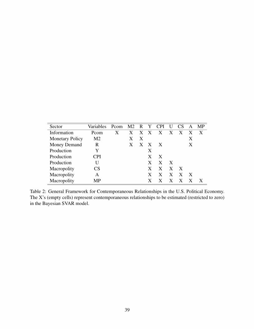
The structure of the contemporaneous relationships that we use—the identification of the A0

matrix—is presented in Table 2. (The matrix A+ allows for all variables to interact via lags.) The

rows of the A0 matrix represent the sectors or equations and the columns are the innovations that

contemporaneously enter each equation. The non-empty cells (marked with X’s) are contempora-

33The reason for these transformations is that our subsequent dynamic responses for the logged variables will all beinterpretable in percentage terms for each variable.

34Note that our sample differs from that used in EMS in two ways. First, we cover a more recent time span than thatused in the their analyses since we include data from 1978–2004. Second, we are working with monthly data, whichmeans our analysis will contain more sampling variability than the aggregated quarterly data used by EMS. We usemonthly data because their arguments imply different reaction times for approval and macropartisanship to changes inthe economy and consumer sentiment.

35The second dummy, for party control, may be weakly endogenous. Future research on the model will try to testfor this possibility.

23

neous structural relationships to be estimated while the empty cells are constrained to be zero.

We must provide a rationale for the contemporaneous restrictions and relationships. Beginning

with the economic sectors, the restrictions for the Information, Monetary Policy, Money Demand

and Production sectors come from the aforementioned studies in macroeconomics. This speci-

fication of the structure of the economy has been found to be particularly useful in the study of

economic policy (see e.g., Sims 1986b, Williams 1990, Robertson and Tallman 2001, Waggoner

and Zha 2003a).36 Next we ask, “which economic equations are affected contemporaneously by

shocks to the political variables?” This is a question about the restrictions to the political shocks

in the economic equations (those in the three right-most columns and first six rows of Table 2).

To allow for political accountability, contemporaneous effects are specified for political variables

in two of the economic equations. First, the macropolity variables—approval, consumer senti-

ment, and macropartisanship can have a contemporaneous effect on commodity prices.37 This is

consistent with recent results in international political economy such as Bernhard and Leblang

(2006). Second, presidential approval is expected to have a contemporaneous effect on interest

rates and on the reaction of the Federal Reserve (Beck 1987, Williams 1990, Morris 2000). The

argument for estimating these structural parameters is that there can be a within-month reaction

by the Federal Reserve to changes in the standing of the presidents who manage their approval.

Finally, we ask “how do economic shocks contemporaneously affect the political variables?” This

is a question about the structure of the last three rows of Table 2. We argue that the real economic

variables—represented by GDP, unemployment, and inflation variables—contemporaneously af-

fect the macropolity. The contemporaneous specification of A0 for the macropolity variables (the

last three rows of Table 2) allows all of the production sector variables to contemporaneously

affect the macropolity variables: innovations in GDP, unemployment, and prices have an imme-

diate effect on consumer sentiment, approval, and macropartisanship. These contemporaneous

36The distinction between contemporaneous and lagged effects is conceived in terms of the speed of response. Forexample, consider shocks in interest rates. Commodity prices respond immediately to these shocks, while it takes atleast a month for firms to adjust their spending to the rise in interest rates. Hence there is a zero restriction for theimpact of R on Y. Again, there is a lagged effect of R on Y and this is captured by A+.

37We thank an earlier reviewer for suggesting the endogenous relationship between macropartisanship and theinformation sector.

24

relationships are suggested by the control variables used in EMS and by related studies of the

economic determinants of public opinion (inter alia, Clarke and Stewart 1995, Clarke, Ho and

Stewart 2000, Green, Palmquist and Schickler 1998). We also specify a recursive contemporane-

ous relationship among the consumer sentiment, approval, and macropartisanship variables. This

is suggested by the discussion of purging in EMS (1998). The blank cells in Table 2 denote the ab-

sence of any contemporaneous impact of the column variables on the row variables. Finally, note

that Σ has (9 × 10)/2 = 45 free parameters and the A0 matrix in Table 2 has 38 free parameters.

Hence, it A0 is over-identified.38

[Table 2 about here.]

The second step in specifying the B-SVAR model is to represent the beliefs about the model’s

parameters. These beliefs are specified by the hyperparameters. EMS and SZ reveal similar beliefs

about the character of the macro-political economy. SZ propose a benchmark prior for empirical

macroeconomics with values of λ1 = 0.1, λ3 = 1, λ4 = 0.1, λ5 = 0.07, and µ5 = µ6 = 5. These

values imply a model with relatively strong prior beliefs about unit roots, some cointegration, but

with little drift in the variables. This prior corresponds to a political economy with strong stochastic

trends and that is difference stationary. This is very similar to EMS’s “running tally” model which

also has stochastic trends but limited drift in the variables. EMS also reveal a belief that some

variables in their political-economic system are cointegrated. Illustrative is EMS’s argument that

macropartisanship is integrated order 1. This reveals a belief the coefficients for the first own lags

of some variables should be unity or that λ1 is small. EMS also express confidence that approval

and consumer sentiment do not have unit roots, which is still possible with these beliefs. We denote

this prior by the name “EMS-SZ Tight”.

Because these hyperparameters are not directly elicited from EMS, it is wise to consider al-

ternative representations of beliefs. A sensitivity analysis is recommended in an investigation like

this, as noted above (Gill 2004, Jackman 2004). We therefore propose two additional prior spec-

38It is also possible to evaluate theoretically implied specifications of A0. In the interest of brevity, we focus in thispaper on the sensitivity of the results to the prior beliefs embodied in the hyperparameters.

25

ifications. The second, allows for more uncertainty than the EMS and SZ prior (larger standard

deviations for the parameters and less weight on the sum of autoregressive coefficients and im-

pact of the initial conditions). We denote this second prior, “EMS-SZ Loose”. The third prior is

a diffuse prior (but still proper so that we can compute posterior densities for various quantities

of interest). The hyperparameters for this final prior represents uninformative or diffuse beliefs

about stochastic trends, stochastic drifts, and cointegration. The hyperparameters for this diffuse

prior allow for large variances around the posterior coefficients, relative to hyperparameters in the

EMS-SZ priors. Thus we analyze the fit of a B-SVAR model with two informed priors and one

uninformed prior. The priors are summarized in the Table 3.

[Table 3 about here.]

3.2 Results

Table 3 presents the log marginal data densities for the three priors. After selecting a model based

on this criteria, we then turn to the dynamic inferences. The interpretation of the B-SVAR model

is dependent on the contemporaneous structure and the prior, but in a way made explicit by the

Bayesian approach. We thus are able to show systematically how our results depend on the beliefs

we bring to the B-SVAR modeling exercise.39 As suggested earlier, the log marginal data density

(log(m(Y ))) is used to compare the prior specifications.40

The final rows of Table 3 report the log marginal data density estimates. The diffuse prior

model has the highest value. But this is not a suitable prior. First, inspection of the results from this

model shows that it overfits the sample data, allowing many non-zero higher order lag coefficients.

This means that impulse responses from this model have implausibly large confidence regions39The additional sensitivity and robustness analysis will be made available with the replication materials for this

article. These auxiliary results support the claims made here.40All posterior fit results are for a posterior sample of 40000 draws with a burnin of 4000 draws using two inde-

pendent chains. The parameters in the two chains pass all standard diagnostic tests—traceplots show good mixing,Geweke diagnostics are insignificant, and Gelman-Rubin psrfs are 1. Thus, we are confident that the sampler has con-verged. The numerical standard error is computing using a Newey-West correction to account for the serial correlationin the Gibbs sampler output as suggested by Geweke (2005, 149, 256) and Chib (1995, 1316). This standard errorsummarizes the numerical accuracy of the simulation of the log marginal data density estimate at the posterior mode,not the variation in the log marginal data density itself.

26

making any dynamic inferences difficult. Second, the log posterior probability of the diffuse prior’s

parameters in the last row of Table 3 is very low meaning that the estimates of the parameters for

this model are very unlikely to have generated the data. Third, the computation of log(m(Y )) in

Equation 8 weights the posterior probability of the data by this probability of the parameters. Since

the parameters have low probability and the in-sample fit is too good, this computation will lead

to an inflated estimate.41 The EMS-SZ Loose prior is better than the EMS-SZ Tight prior based

on the log(m(Y )) values of the log marginal data density. The former generates a posterior with

a larger log(m(Y )) than the EMS-SZ Tight prior. The log Bayes factor which compares the two

prior specifications is 836, indicating a strong preference for the Loose prior over the Tight prior.

For each of the three priors in Table 3 we computed the impulse responses for the full nine

equation system. Based on the log(m(Y )) and impulse responses, we present the results for the

EMS-SZ Loose prior. The model with the EMS-SZ Loose prior produces the most theoretically

meaningful dynamics. The impulse responses for the diffuse prior model have error bands than are

vary widely and make interpretation of the magnitudes and direction of the dynamics impossible.

The results for the two informed priors differ in a reasonable way. The responses to shocks in with

the EMS-SZ Tight prior are more permanent and dissipate more slowly than those in the EMS-SZ

Loose prior, as expected. The latter allows for more variance in the parameters and more rapid lag

decay (and thus faster equilibration to shocks than with the EMS-SZ Tight prior).42

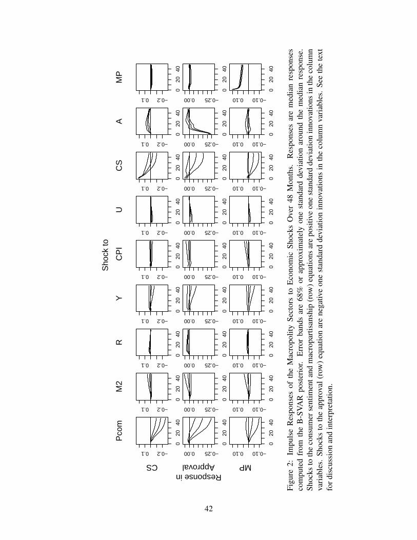
We focus on two sets of impulse responses for the model with the EMS-SZ Loose prior. The

first are the responses of the economy to changes in politics. Figure 1 presents the subset of the

41As Chib (1995) notes, the quantity in Equation 8 is the log of the basic marginal likelihood identity or

m(Y ) =Pr(Y |A0, A+)Pr(A0, A+)

Pr(A0, A+|Y )

For the diffuse prior model, the posterior probability of the parameters in the denominator, Pr(A0, A+|Y ) will besmall. This will then (incorrectly) inflate the computation of m(Y ) and hence its logarithm. This is evidence in Table3 where the log(Pr(A0, A+|Y )) is much larger (in absolute value) for the diffuse prior than for the informed priors.The log prior term, log(Pr(A0, A+)), for the models are similar in magnitude across the models and negative in sign.Thus it is the poor posterior fit of parameters that generates the anomalously larger log(m(Y )) for the diffuse priormodel. This is a pitfall of using too loose a prior for the B-SVAR model.

42Space restrictions do not allow us to report the many impulse responses we produced. A full collection of them isavailable in the replication materials for this paper.

27

responses of the economic equations to shocks in the macropolity sector variables.43 Each row

are the responses for the indicated equation for a shock in the column variable. Responses are

median estimates with 68% confidence region error bands, computed pointwise over a 48 month

time horizon.44 The interpretation of the impulse responses differs from those typically seen in

the literature. In standard reduced form VAR models with a recursive identification of the con-

temporaneous error covariance, one analyzes the responses to positive shocks to each equation in

the system. Such a normalization of the shocks is not possible in non-recursive B-SVAR mod-

els (Waggoner and Zha 2003b). This is because there is no unique correspondence of shocks to

equations in a simultaneous system like an SVAR. Thus positive shocks to one equation may im-

ply negative shocks to other equations (e.g., structural shocks to the inflation and unemployment

equations should have opposite signs because of their Philips’ curve relationship).

[Figure 1 about here.]

The responses of the economy to shocks in the macropolity variables indicate that changes in

public opinion and expectations do have predictable and sizeable effects on the economy. Shocks

enter the commodity price (Pcom) equation positively, so that increases in consumer sentiment lead

to lagged increases in commodity prices, reaching a maximum of 0.1% over 30 months. Similarly,

increases in approval generate less than 0.05% decreases in commodity prices. With respect to

the monetary policy and money demand sectors (M2 and R), changes in consumer sentiment and

approval affect interest rates, but not monetary policy. These shocks enter the interest rate equation

negatively so declines in consumer sentiment increase interest rates (with the lower edge of the

68% confidence region at zero) while declines in approval lead to lower interest rates over 10-

12 months. Thus, consumer sentiment (presidential approval) and interest rates are positively43These responses were generated using the Gibbs sampler for B-SVAR model in Waggoner and Zha (2003a). This

Gibbs sampler draws samples from the posterior distribution of the restricted (over-identified) A0 matrix and then fromthe autoregressive parameters of the model. These draws are then used to construct the impulse responses (Brandt andFreeman 2006). The responses have been scaled by a factor of 100, so they are in percentage point terms. We employa posterior based on 20000 draws after a burnin of 2000 draws. Similar results were obtained for a posterior sampletwice as large using two independent MCMC chains.

44Sims and Zha (1999) argue that 68% error bands (which are approximately one standard deviation bands on eachside of the mode) provide a better summary of the central tendency or likelihood of the impulse responses. Furtherdiscussion and examples of why this is a preferable confidence region can be found in Brandt and Freeman (2006).

28

(negatively) related. Note that the consumer sentiment shock generates an interest rate response

that is nearly twice as large and in the opposite direction of the approval shock over 48 months.

The interest rate and money responses are consistent with political monetary cycle arguments

that presidents attempt to manage their approval by strengthening the economy; the Fed works

counter-cyclically to reduce inflation and unemployment both of which also move in the expected

directions to approval shocks (Beck 1987, Williams 1990). These responses are consistent with

the idea of political accountability where policy responds to public perceptions of the president.

For the production sectors—real GDP (Y), inflation (CPI), and unemployment (U)—the po-

litical shocks generate responses as well. Real GDP does not respond to political shocks, as the

confidence regions are large and cover zero. Positive shocks in consumer sentiment and approval

lead to higher inflation as the CPI responses to these shocks increase, albeit with a lag. Note

though that these responses are small—always less than 0.008%. The median total response of

CPI to the consumer sentiment and approval innovations over 48 months is less than 0.2%.45 The

shocks to the unemployment equation enter negatively, so decreases in consumer sentiment lower

unemployment by at most 0.05% with a lag over 48 months. Over 48 months the median to-

tal response of unemployment to innovations in consumer sentiment is a -1.82 point decline in

unemployment (68% credible interval [-2.03, -1.62]). Similarly, declines in approval increase un-

employment, peaking at about a 0.02% change around 10 months and then declining to zero at 48

months. These are possibly some expectational responses as both variables are trending. Thus,

even the non-zero effects of the macropolity on the real economy are weak.

The other side of the B-SVAR system are the impacts of the economy on the macropolity.

Figure 2 present the full set of responses for the macropolity equations. Here we can judge the

relative impacts of different economic and political shocks on consumer sentiment, approval, and

macropartisanship. In the consumer sentiment and macropartisanship equations the response to

their own shocks is positive so shocks enter these equations as positive one standard deviation

changes. In contrast, the approval equation the response to its own shock is negative so shocks enter

45This median total impulse response is found by cumulating the MCMC sample of each impulse response and thensummarizing its median and credible interval.

29

this equation as negative one standard deviation changes. Thus each plot in the figure is the impact

of a signed one standard deviation change in the column variable to the row equation. Consumer

sentiment responds most strongly to commodity price and approval shocks. One standard deviation

increases in commodity prices (in percentage terms, about 0.25%) lowers consumer sentiment by

a maximum of 0.17 points over 48 months. In cumulative terms, this same increase in commodity

prices lowers the median consumer sentiment by a full 4.5 points (68% credible interval [-6.98,

-2.21]) over 48 months. In contrast, the one standard deviation increase in presidential approval

raises consumer sentiment a median total impact 1.96 points over 48 months (68% credible region

[1.28, 2.71]).

[Figure 2 about here.]

Commodity prices, consumer sentiment and approval’s own innovations have the largest im-

pact on approval responses. A one standard deviation negative shock to commodity prices lowers

approval by a maximum of 0.15 points over 48 months. This cumulates to a median total change

of nearly -3.5 points for an initial quarter percent drop in commodity prices (68% credible inter-

val [-6.35, -0.79]). Thus, information markets have a wide degree of influence on both consumer

sentiment and approval. The effect of consumer sentiment shocks on approval reflects this as well.

The magnitude of the median total effect of the impact of consumer sentiment on approval is large.

Over 48 months, a one standard deviation drop in consumer sentiment lowers approval by a total

median impact of -1.6 points; at 48 months the probability that the cumulative response of approval

to the consumer sentiment shock is negative is 0.73. Thus, innovations in information markets im-

pact consumer sentiment and approval and then the impacts on consumer sentiment feed-forward

into subsequent approval changes. Note however that the real economy does not have impacts on

any of the macropolity variables.

Consider next the responses of the macropolity sector. These results differ from those previ-

ously seen in the literature (cf., EMS, Chapter 10) because they are the result of embedding the

macropolity in a full model of the political economy. Consumer sentiment responds mainly to

its own shocks and not those of the other political variables (not even with a lag). The consumer

30

sentiment response to approval shocks is small over 48 months. Neither consumer sentiment nor

approval respond to changes in macropartisanship.

One of the main questions for both our analysis and for EMS is the exploration of what moves

aggregate partisanship? The final row of plots in Figure 2 shows the responses for the macropar-

tisanship equation. Positive shocks in the production sector and in presidential approval have no

sizeable impact on aggregate partisanship. The response of macropartisanship to positive one stan-

dard deviation shocks in commodity prices and consumer sentiment are suggestive, but weak. Over

48 months the positive commodity price and consumer sentiment shocks lower macropartisanship

by only about 0.05%. The impact of these shocks on macropartisanship does not cumulate to even

a one point change over 48 months. In the end, the macropartisanship equation is mainly driven

by shocks to macropartisanship itself.

4 Conclusion

Political scientists need to learn how to specify B-SVAR models. Translating beliefs into the con-

temporaneous relationships in A0 appears straightforward. Careful study of the literature on topics

like macropartisanship usually reveals how researchers conceive of some of these relationships.

Admittedly, scholars often do not mention some contemporaneous relationships and it is not clear

that setting them to zero is reasonable. But the virtue of the structural VAR approach is that it

allows us to estimate whether the respective contemporaneous coefficient should be unrestricted.

Using a Bayesian approach also allows us to summarize our uncertainty about such contempora-

neous restrictions. In addition, we need to learn how to specify the hyperparameters. Scholars

sometimes are not clear about their beliefs about all of these parameters. How much sampling

error should be discounted via the choice of λ0 is another issue. In recent years political methodol-

ogists have produced a number of useful findings about the persistence properties of political data.

However, macroeconomists are far ahead of us in this regard. They have much more experience

in translating their arguments and experience in fitting B-SVAR models into clusters of hyperpa-

31

rameters. An important part of this experience comes from years of attempting to forecast the

macroeconomy. The efforts to forecast the macropolity and international relations, are, for myriad

reasons, less well developed in our discipline.46

Important extensions of the B-SVAR model are being developed. For example, there are new

methods for translating theory into additional restrictions on the effects of lagged endogenous

variables (the A+ matrix in the model) and for formally testing these restrictions (e.g., Cushman

and Zha 1997). Some researchers contend that formal models produce more useful structural

insights than VAR models (structural, reduced form and/or Bayesian). Proponents of Bayesian time

series models reply that formal models often suffer from problems of observational equivalence

and that they are very difficult to fit to data. A more catholic approach is taken by Sims (2005)

who argues that formal models—in the case of macroeconomics, Dynamic Stochastic General

Equilibrium (DSGE) models—are good for “spinning stories” and that these stories ought to be

restrained or refined by the results of VARs. Work is underway in macroeconomics to try to make

this connection more explicit. This work specifically uses DSGE models to develop informed

priors for B-SVAR models. The DSGE models are linearized at the point representing general,

macroeconomic equilibrium and then the parameter values from the DSGE model are translated

into the hyperparameters of the B-SVAR model.47

In political science we lack a well developed, general equilibrium theory of the kind that

spawned DSGE models. However, spatial theory and the new works on electoral coordination

and campaign finance (Mebane 2000, Mebane 2003, Mebane 2005) point the way to the devel-

opment of such theory. The challenge is to join these works with the B-SVAR approach to make

more sustained progress in study of the macropolity.48

46Perhaps this is why most Bayesians in political science employ uninformed priors. On this point see Brandt andFreeman (2006).

47Ingram and Whiteman (1994) and Del Negro and Schorfheide (2004) draw informed priors from DSGEs forBVARs. Leeper et al. (1996) argue that DSGE models provide insights into the long-term economic dynamics andVARs into the short-term dynamics of the economy. In a more recent article, Sims (2005) notes that DSGE models arebetter than VARs for “spinning elaborate stories about how the economy works” but expresses some skepticism aboutwhether linearizations of DSGE models usually produce accurate second order approximations to the likelihood. Hegoes on to say, “No one is thinking about the time varying residual variances when they specify or calibrate these[DSGE] models.” Sims predicts a “hornet’s nest” for macroeconomic DSGE policy modelers.

48For a sketch of how this development might occur see Freeman (2005).

32

ReferencesAlesina, Alberto and Howard Rosenthal. 1995. Partisan Politics, Divided Government and the

Economy. Cambridge: Cambridge University Press.

Alesina, Alberto, John Londregan and Howard Rosenthal. 1993. “A Model of the Political Econ-omy of the United States.” American Political Science Review 87:12–33.

Bartels, Larry M. 1991. “Instrumental and “Quasi-Instrumental” Variables.” American Journal ofPolitical Science 35(3):777–800.

Beck, Nathaniel. 1987. “Elections and the Fed: Is there a Political Monetary Cycle?” AmericanJournal of Political Science 31(1):194–216.

Bernanke, B. 1986. Alternative explanations of the money-income correlation. In Carnegie-Rochester Conference Series on Public Policy. Amsterdam: North-Holland.

Bernardo, Jose M. 1979. “Reference Posterior Distributions for Bayesian Inference.” Journal ofthe Royal Statistical Society. Series B (Methodological) 41(2):113–147.

Bernhard, William and David Leblang. 2006. Democratic Processes and Financial Markets: Pric-ing Politics. New York: Cambridge University Press.

Blanchard, O. and D. Quah. 1989. “The dynamic effects of aggregate demand and supply distur-bances.” American Economic Review 79:655–673.

Box-Steffensmeier, Janet M. and Renee M. Smith. 1996. “The Dynamics of Aggregate Partisan-ship.” American Political Science Review 90(3):567–80.

Brandt, Patrick T. and John R. Freeman. 2006. “Advances in Bayesian Time Series Modeling andthe Study of Politics: Theory Testing, Forecasting, and Policy Analysis.” Political Analysis14(1):1–36.

Brandt, Patrick T. and John T. Williams. 2007. Multiple Time Series Models. Beverly Hills: Sage.

Brandt, Patrick T., Michael Colaresi and John R. Freeman. 2006. “Reci-procity, Accountability and Credibility In International Relations.”.http://www.utdallas.edu/ pbrandt/working/BCF20060531.pdf.

Carlin, Bradley P. and Thomas A. Louis. 2000. Bayes and Empirical Bayes Methods for DataAnalysis. 2nd ed. Chapman & Hall/CRC.

Chib, Siddartha. 1995. “Marginal Likelihood from the Gibbs Output.” Journal of the AmericanStatistical Association 90(432):1313–1321.

Clarke, Harold D., Karl Ho and Marianne C. Stewart. 2000. “Major’s lesser (not minor) effects:prime ministerial approval and governing party support in Britain since 1979.” Electoral Stud-ies 19(2–3):255–273.

33

Clarke, Harold D. and Marianne C. Stewart. 1995. “Economic Evaluations, Prime MinisterialApproval and Governing Party Support: Rival Models Reconsidered.” British Journal of Po-litical Science 25(2):145–170.

Cortes, Fernando, Adam Przeworski and John Sprague. 1974. System Analysis for Social Scientists.New York: John Wiley and Sons.

Cushman, David O. and Tao Zha. 1997. “Identifying Monetary Policy in a Small Open EconomyUnder Flexible Exchange Rates.” Journal of Monetary Economics 39:433–448.

DeBoef, Suzanna and James Granato. 1997. “Near Integrated Data and the Analysis of PoliticalRelationships.” American Journal of Political Science 41(2):619–640.

DeBoef, Suzanna and Luke Keele. 2006. “Dynamic Specification Revisited.”http://polisci.la.psu.edu/faculty/DeBoef/post-polmeth20.pdf.

Del Negro, Marco and Frank Schorfheide. 2004. “Priors From General Equilibrium Models forVARs.” International Economic Review 45:643–673.

Doan, Thomas, Robert Litterman and Christopher Sims. 1984. “Forecasting and Conditional Pro-jection Using Realistic Prior Distributions.” Econometric Reviews 3:1–100.

Erikson, Robert S., Michael B. MacKuen and James A. Stimson. 1998. “What Moves Macroparti-sanship? A Response to Green, Palmquist and Schickler.” American Political Science Review92(4):901–912.

Erikson, Robert S., Michael B. MacKuen and James A. Stimson. 2002. The Macropolity. NewYork: Cambridge University Press.

Franzese, Robert F. 2002. Macroeconomic Policies of Developed Democracies, Cambridge Studiesin Comparative Politics. Cambridge University Press.

Franzese, Robert F. and Jude Hays. 2005. “Empirical Modeling Strategies for Spatial Interde-pendence: Omitted Variable vs. Simultaneity Bias.” Paper originally presented at the AnnualMeeting of the Political Methodology Society, Stanford University.

Freeman, John R. 2005. “Modeling Macropolitics: EITM and Reality.” Paper presented at theEITM Workshop, Canadian Political Science Association Meetings, London, Ontario.

Freeman, John R., John T. Williams, Daniel Houser and Paul Kellstedt. 1998. “Long MemoriedProcesses, Unit Roots and Causal Inference in Political Science.” American Journal of Polit-ical Science 42(4):1289–1327.

Freeman, John R., John T. Williams and Tse-Min Lin. 1989. “Vector Autoregression and the Studyof Politics.” American Journal of Political Science 33:842–77.

Geweke, John. 2005. Contemporary bayesian Econometrics and Statistics. John Wiley & Sons.

Gill, Jeff. 2002. Bayesian Methods: A Social and Behavioral Sciences Approach. Boca Raton:Chapman and Hall.

34

Gill, Jeff. 2004. “Introducing the Special Issue of Political Analysis on Bayesian Methods.” Polit-ical Analysis 12(4):323–337.

Goldstein, Joshua and Jon C. Pevehouse. 1997. “Reciprocity, Bullying and International Coop-eration: Time Series Analysis of the Bosnian Conflict.” American Political Science Review91:515–524.

Goldstein, Joshua S., Jon C. Pevehouse, Deborah J. Gerner and Shibley Telhami. 2001. “Reci-procity, Triangularity, and Cooperation in the Middle East, 1979-1997.” Journal of ConflictResolution 45(5):594–620.

Green, Donald, Bradley Palmquist and Eric Schickler. 1998. “Macropartisanship: A Replicationand Critique.” American Political Science Review 92(4):883–900.

Hamilton, James D. 1994. Time Series Analysis. Princeton: Princeton University Press.

Ingram, Beth F. and Charles H. Whiteman. 1994. “Supplanting the ‘Minnesota’ prior: ForecastingMacroeconomic Time Series Using Real Business Cycle Model Priors.” Journal of MonetaryEconomics 34:497–510.

Jackman, Simon. 2004. “Bayesian Analysis in Political Science.” Annual Reviews of PoliticalScience 7:483–505.

Jackman, Simon. in progress. Bayesian Analysis for the Social Sciences. Hoboken, New Jersey:John Wiley & Sons.

Kadiyala, K. Rao and Sune Karlsson. 1997. “Numerical Methods For Estimation and Inference inBayesian VAR-Model.” Journal of Applied Econometrics 12:99–132.

Leeper, Eric M., Christopher A. Sims and Tao A. Zha. 1996. “What Does Monetary Policy Do?”Brookings Papers on Economic Activity 1996(2):1–63.

Litterman, Robert. 1980. Techniques for forecatsing with vector autoregressions PhD thesis Uni-versity of Minnesota.

Manski, Charles. 1995. Identification Problems in the Social Sciences. Cambridge: HarvardUniversity Press.

Martin, Andrew and Kevin Quinn. 2002. “Dynamic Ideal Point Estimation via Markov ChainMonte Carlo for the U.S. Supreme Court.” Political Analysis 10(2):134–153.

Mebane, Walter R. 2000. “Coordination, Moderation, and Institutional Balancing in AmericanPresidential and House Elections.” American Political Science Review 94:37–53.

Mebane, Walter R. 2003. Congressional Campaign Contributions, Direct Service, and ElectoralOutcomes in the United States: Statistical Tests of a Formal Game Model With StatisticalEstimates. In Political Complexity: Nonlinear Models of Politics, ed. Diana Richards. AnnArbor, Michigan: University of Michigan Press.

35

Mebane, Walter R. 2005. “Partisan Messages, Unconditional Strategies, and Coordination inAmerican Elections.” Revised version of a paper originally presented at the Annual Meet-ing of the Political Metholodolgy Society, Stanford University.

Morris, Irwin L. 2000. Congress, the President, and the Federal Reserve: The Politics of AmericanMonetary Policy-Making. Ann Arbor: University of Michigan Press.

Ogata, Ktsuhiko. 1967. State Space Analysis of Control Systems. Englewood Cliffs, NJ: Prentice-Hall, Inc.

Ostrom, Charles and Renee Smith. 1993. “Error Correction, Attitude Persistence, And ExecutiveRewards and Punishments: A Behavioral Theory of Presidential Approval.” Political Analysis3:127–184.

Pevehouse, Jon C. and Joshua S. Goldstein. 1999. “Serbian Compliance or Defiance in Kosovo?Statistical Analysis and Real-Time Predictions.” Journal Of Conflict Resolution 43(4):538–546.

Poole, Keith. 1998. “Recovering a Basic Space From a Set of Issue Scales.” American Journal ofPolitical Science 42:954–993.

Poole, Keith T. and Howard Rosenthal. 1997. Congress: A Political-Economic History of Roll CallVoting. New York: Oxford University Press.

Robertson, John C. and Ellis W. Tallman. 1999. “Vector Autoregressions: Forecasting And Real-ity.” Economic Review (Atlanta Federal Reserve Bank) 84(1):4–18.

Robertson, John C. and Ellis W. Tallman. 2001. “Improving Federal Funds rate forecasts in VARmodels used for policy analysis.” Journal of Business and Economics Statistics 19(3):324–330.

Sims, Christopher A. 1980. “Macroeconomics and Reality.” Econometrica 48(1):1–48.

Sims, Christopher A. 1986a. “Are forecasting models usable for policy analysis?” QuarterlyReview, Federal Reserve Bank of Minneapolis 10:2–16.

Sims, Christopher A. 1986b. “Specification, Estimation, and Analysis of Macroeconomic Models.”Journal of Money, Credit and Banking 18(1):121–126.

Sims, Christopher A. 2005. “The State of Macroeconomic Policy Modeling: Where Do We GoFrom Here?” “Macroeconomics and Reality, 25 Years Later” Conference, Barcelona, Spain,http://www.econ.upf.es/crei/activities/sc conferences/22/Papers/sims.pdf.

Sims, Christopher A. and Tao A. Zha. 1995. “Error Bands for Impulse Responses.”http://sims.princeton.edu/yftp/ier/.

Sims, Christopher A. and Tao A. Zha. 1998. “Bayesian Methods for Dynamic Multivariate Mod-els.” International Economic Review 39(4):949–968.

36

Sims, Christopher A. and Tao A. Zha. 1999. “Error Bands for Impulse Responses.” Econometrica67(5):1113–1156.

Theil, Henri. 1963. “On the Use of Incomplete Prior Information in Regression Analysis.” Journalof the American Statistical Association 58(302):401–414.

Waggoner, Daniel F. and Tao A. Zha. 2003a. “A Gibbs sampler for structural vector autoregres-sions.” Journal of Economic Dynamics & Control 28:349–366.

Waggoner, Daniel F. and Tao A. Zha. 2003b. “Likelihood Preserving Normalization in MultipleEquation Models.” Journal of Econometrics 114:329–347.

Williams, John T. 1990. “The Political Manipulation of Macroeconomic Policy.” American Politi-cal Science Review 84(3):767–795.

Williams, John T. 1993. “What Goes Around Comes Around: Unit Root Tests and Cointegration.”Political Analysis 1:229–235.

Zellner, A. and A. Siow. 1980. Posterior odds for selected regression hypotheses. In BayesianStatistics I, ed. J.M. Bernardo et al. Valencia University Press pp. 585–603.

Zha, Tao A. 1998. “A Dynamic Multivariate Model for the Use of Formulating Policy.” EconomicReview (Federal Reserve Bank of Atlanta) 83(1):16–29.

Zha, Tao A. 1999. “Block recursion and structural vector autoregression.” Journal of Econometrics90:291–316.

37

Parameter Range Interpretationλ0 [0,1] Overall scale of the error covariance matrixλ1 > 0 Standard deviation about A1 (persistence)λ2 = 1 Weight of own lag versus other lagsλ3 > 0 Lag decayλ4 ≥ 0 Scale of standard deviation of interceptλ5 ≥ 0 Scale of standard deviation of exogenous variables coefficientsµ5 ≥ 0 Sum of autoregressive coefficients componentµ6 ≥ 0 Correlation of coefficients/Initial condition component

Table 1: Hyperparameters of Sims-Zha Reference Prior

38

Sector Variables Pcom M2 R Y CPI U CS A MPInformation Pcom X X X X X X X X XMonetary Policy M2 X X XMoney Demand R X X X X XProduction Y XProduction CPI X XProduction U X X XMacropolity CS X X X XMacropolity A X X X X XMacropolity MP X X X X X X

Table 2: General Framework for Contemporaneous Relationships in the U.S. Political Economy.The X’s (empty cells) represent contemporaneous relationships to be estimated (restricted to zero)in the Bayesian SVAR model.

39

Hyp

erpa

ram

eter

EM

S-SZ

Tigh

tE

MS-

SZL

oose

Diff

use

Err

orco

vari

ance

mat

rix

scal

e(λ

0)

0.6

0.6

1St

anda

rdde

viat

ion

ofA

1(p

ersi

sten

ce)(

λ1)

0.1

0.15

10D

ecay

ofla

gva

rian

ces(λ

3)

11

0St

anda

rdde

viat

ion

ofin

terc

ept(

λ4)

0.1

0.15

10St

anda

rdde

viat

ion

ofex

ogen

ous

vari

able

s(λ

5)

0.07

0.07

10Su

mof

auto

regr

essi

veco

effic

ient

sco

mpo

nent

(µ5)

52

0C

orre

latio

nof

coef

ficie

nts/

Initi

alco

nditi

onco

mpo

nent

(µ6)

52

0lo

g(m

(Y))

1136

812

204

1921

6N

umer

ical

stan

dard

erro

rofl

og(m

(Y))

0.03

0.01

0.25

log(P

r(A

0,A

+|Y

))-4

378

-521

0-1

1158

Tabl

e3:

Four

B-S

VAR

prio

rsan

dth

eirp

oste

rior

fitm

easu

res

40

0 10 30

−0.

100.

050.

20

Pco

m

CS

0 10 30

−0.

20.

2

M2

0 10 30

−0.

020.

02

R

0 10 30

−0.

010

0.01

0

Y

0 10 30

0.00

00.

010

CP

I

0 10 30

−0.

060.

00

U

0 10 30

−0.

100.

050.

20

Approval

0 10 30

−0.

20.

2

0 10 30

−0.

020.

02

0 10 30

−0.

010

0.01

0

0 10 30

0.00

00.

010

0 10 30

−0.

060.

00

0 10 30

−0.

100.

050.

20

MP

0 10 30

−0.

20.

20 10 30

−0.

020.

02

0 10 30

−0.

010

0.01

0

0 10 30

0.00

00.

010

0 10 30

−0.

060.

00

Res

pons

e in

Shock to

Figure 1: Impulse Responses of the Economic Sectors to Political Shocks Over 48 Months. Re-sponses are median responses computed from the B-SVAR posterior. Error bands are 68% orapproximately one standard deviation around the median response. Shocks to the Pcom, M2, Y,and CPI (row) equations are positive one standard deviation innovations in the column variables.Shocks to the R and U (row) equations are negative one standard deviation innovations in thecolumn variables. See the text for discussion and interpretation.

41

020

40

−0.20.1

CS

Pco

m

020

40

−0.250.00

Approval

020

40

−0.100.10

MP

020

40

−0.20.1

M2

020

40

−0.250.00

020

40

−0.100.10

020

40−0.20.1

R

020

40

−0.250.00

020

40

−0.100.100

2040

−0.20.1

Y

020

40−0.250.00

020

40

−0.100.10

020

40

−0.20.1

CP

I

020

40

−0.250.00

020

40

−0.100.10

020

40

−0.20.1

U

020

40

−0.250.00

020

40

−0.100.10

020

40

−0.20.1

CS

020

40

−0.250.00

020

40

−0.100.10

020

40

−0.20.1

A

020

40

−0.250.00

020

40

−0.100.10

020

40

−0.20.1

MP

020

40

−0.250.00

020

40

−0.100.10

Response in

Sho

ck to

Figu

re2:

Impu

lse

Res

pons

esof

the

Mac

ropo

lity

Sect

ors

toE

cono

mic

Shoc

ksO

ver

48M

onth

s.R

espo

nses

are

med

ian

resp

onse

sco

mpu

ted

from

the

B-S

VAR

post

erio

r.E

rror

band

sar

e68

%or

appr

oxim

atel

yon

est

anda

rdde

viat

ion

arou

ndth

em

edia

nre

spon

se.

Shoc

ksto

the

cons

umer

sent

imen

tand

mac

ropa

rtis

ansh

ip(r

ow)e

quat

ions

are

posi

tive

one

stan

dard

devi

atio

nin

nova

tions

inth

eco

lum

nva

riab

les.

Shoc

ksto

the

appr

oval

(row

)eq

uatio

nar

ene

gativ

eon

est

anda

rdde

viat

ion

inno

vatio

nsin

the

colu

mn

vari

able

s.Se

eth

ete

xtfo

rdis

cuss

ion

and

inte

rpre

tatio

n.

42