1.7 Separation of Total Power Losses ............................................................................ 12
1.7.1 Hysteresis Loss ....................................................................................................... 13
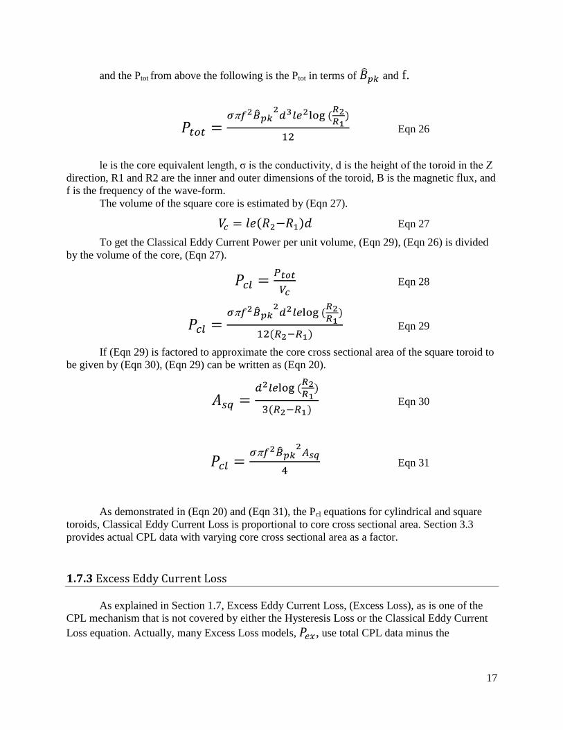
1.7.2 Classical Eddy Current Loss .................................................................................. 13
1.7.3 Excess Eddy Current Loss ...................................................................................... 17 Section 2 Experimental Data Collection Method and Design .......................................... 19
2.0 Required Experiments to achieve thesis goals ....................................................... 19
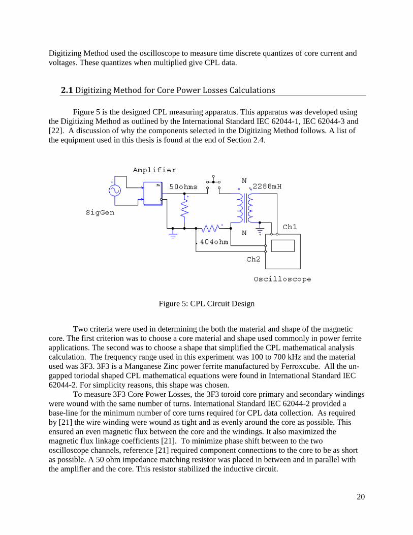
2.1 Digitizing Method for Core Power Losses Calculations ......................................... 20
2.7 Accuracy of Matrix and MATLAB Best Fit Method ................................................. 35 Section 3 Core Power Loss Equation Evaluation ............................................................. 39
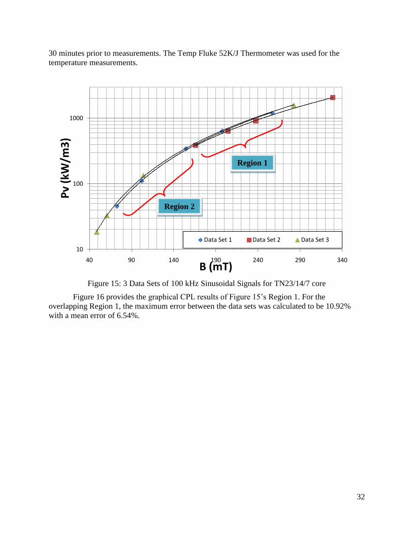
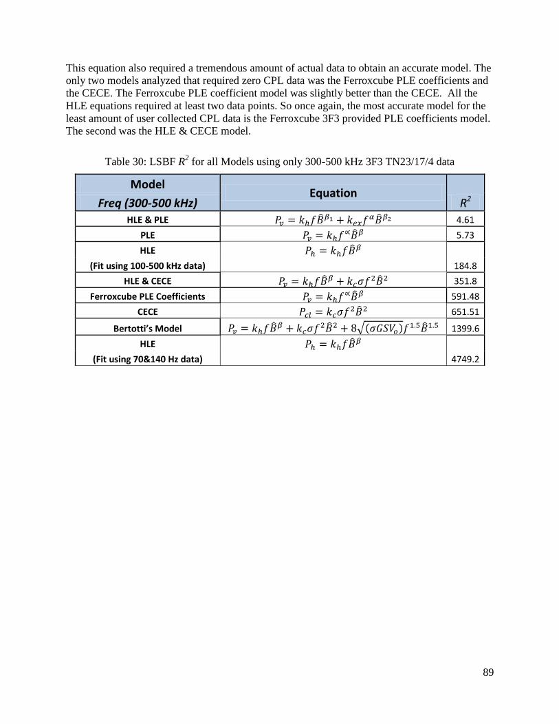
3.0 Results of Empirical Equation Component Verification ........................................ 39
3.1 The Validity of the Hysteresis Loss Equation for Low Frequencies ..................... 39
3.2 Conductivity in an Electrical Field ........................................................................... 45
3.3 Core Area as a factor in CPL per volume Equations ............................................... 51 Section 4 CPL Data Fitting and Statistics Analysis .......................................................... 61
4.2 Power Law Equation (PLE) ...................................................................................... 64
4.3 Hysteresis Loss Equation.......................................................................................... 71
4.4 Classical Eddy Current Equation (CECE) ................................................................. 76
4.5 Separation of Total Power Losses Models .............................................................. 78
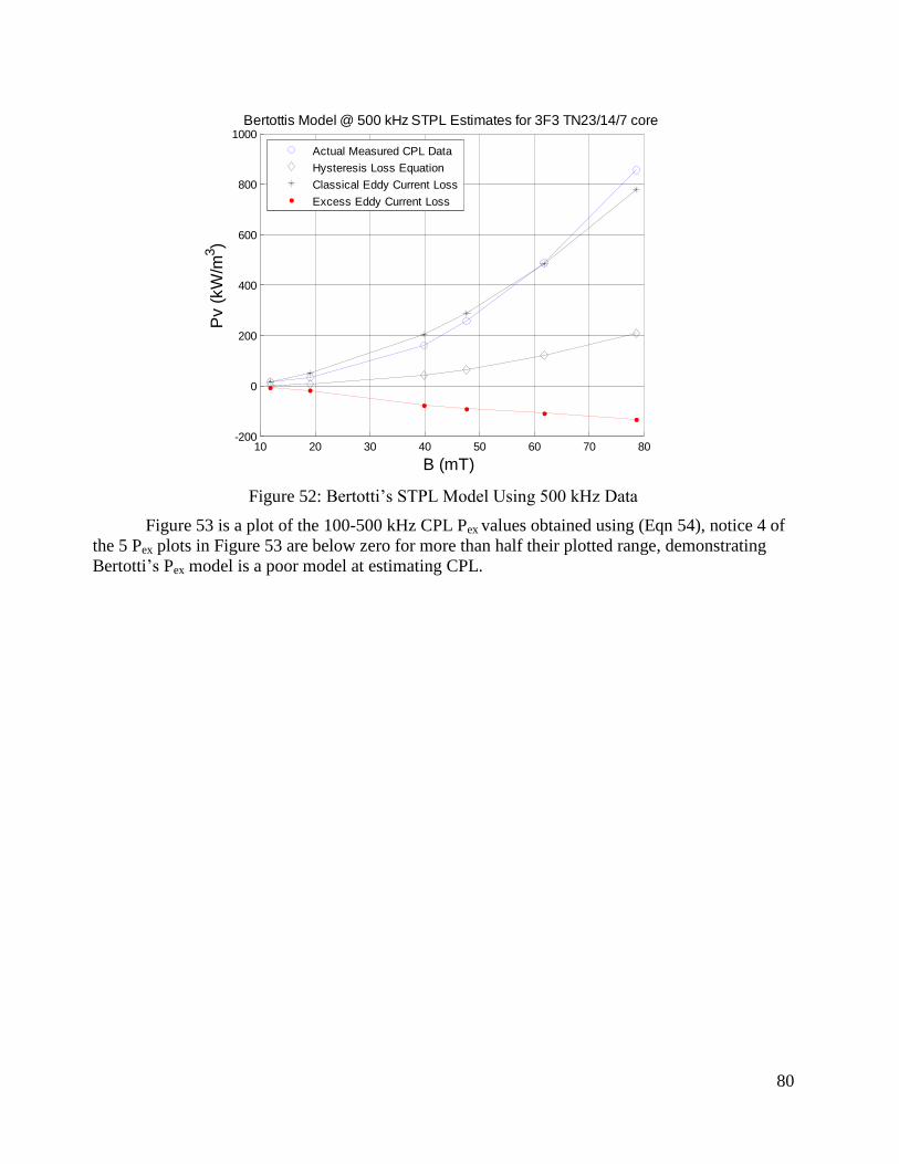
4.5.1 Bertotti’s Model ...................................................................................................... 78
4.5.2 Hysteresis Loss Equation and Classical Eddy Current Equation ....................... 84
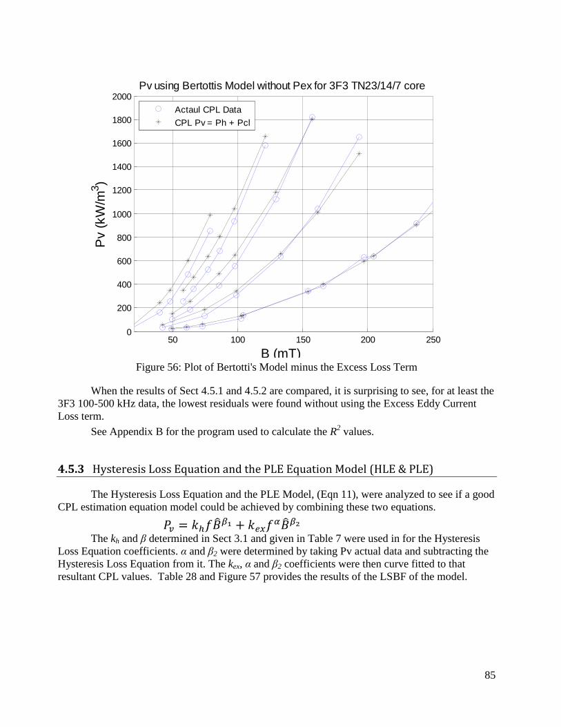
4.5.3 Hysteresis Loss Equation and the PLE Equation Model .................................... 85 Section 5 Conclusions ....................................................................................................... 88
List of References ............................................................................................................. 90 Appendix A: MATLAB CODE ....................................................................................... 92 Appendix B: CPL Collected Data .................................................................................. 105
iii
List of Figures
Figure 1: Domain Wall Theory, adapted from figures in Reference [1] and [2] ................ 8 Figure 2: Hysteresis Loop at 100kHz and @ 273mT ......................................................... 9 Figure 3: 3D Cylinder for Pc derivation ........................................................................... 14
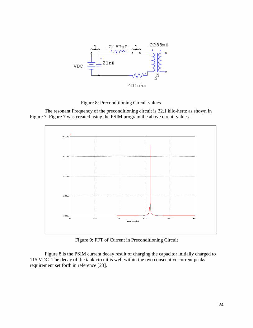
Figure 4: Rectangular toroidal Core Figure [40] .............................................................. 16 Figure 5: CPL Circuit Design ........................................................................................... 20 Figure 6: Ring Toroid ....................................................................................................... 21 Figure 7: Preconditioning Circuit ..................................................................................... 23 Figure 9: FFT of Current in Preconditioning Circuit ........................................................ 24
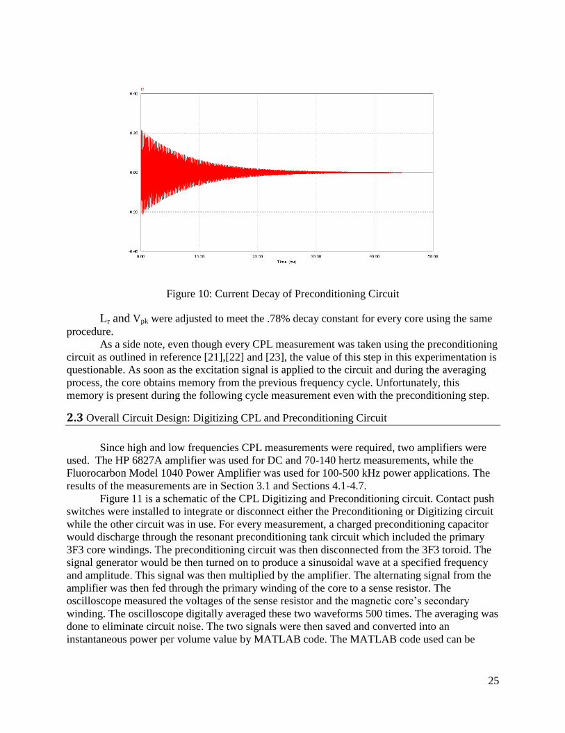
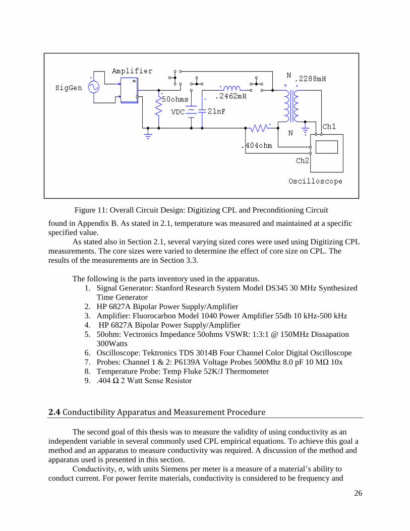
Figure 8: Preconditioning Circuit values .......................................................................... 24 Figure 10: Current Decay of Preconditioning Circuit....................................................... 25 Figure 11: Overall Circuit Design: Digitizing CPL and Preconditioning Circuit ............ 26 Figure 12: Conductivity Apparatus ................................................................................... 28 Figure 13: Current and Voltage of Conductivity of the plate ........................................... 29
Figure 15: 3 Data Sets of 100 kHz Sinusoidal Signals for TN23/14/7 core ..................... 32 Figure 16: Region 1 of 3 Data Sets of 100 kHz Sinusoidal Signals for TN23/14/7 core . 33
Figure 17: Region 2 of 3 Data Sets of 100 kHz Sinusoidal Signals for TN23/14/7 core . 34 Figure 18: Validation of MATLAB Code Picture ............................................................ 35 Figure 19: Core Power Loss Test Fixture used in Hysteresis Loss Equation ................... 40
Figure 20: Hysteresis Loss at 70 Hertz ............................................................................. 41 Figure 21: 70 & 140 Hertz graph using 70 Hertz Best Fit Coefficients ........................... 42
Figure 22: PLE for 70 and 140 Hertz with α constrained to 1 .......................................... 43 Figure 23: PLE for 70 and 140 Hertz with α unconstrained ............................................. 44 Figure 24: Conductivity Apparatus ................................................................................... 45
Figure 25: AC Conductivity vs varying AC Electric Field............................................... 47 Figure 26: DC Conductivity vs Electric Field .................................................................. 47
Figure 27: Voltage and Current of the 3F3 PLT 48/38/4 σ measurements ...................... 49 Figure 28: 3F3 Plate Capacitance vs Freq ........................................................................ 50
Figure 29: Phase Angle vs Freq ........................................................................................ 51 Figure 30: Resistance vs Freq for 3F3 Plate Measurement .............................................. 51
Figure 33: 3F3 TN 23/14/7 same size core lot Variability ............................................... 54 Figure 34: Core Area effects on Core Loss ...................................................................... 55 Figure 35: Core Area CPL Losses for 100 khz ................................................................. 56 Figure 36: Core Area CPL Losses for 500 khz ................................................................. 57 Figure 37: Hysteresis Loss Equation for 70 Hertz ............................................................ 62
Figure 38: Low Frequency Core Power Loss for TN 23/14/7 .......................................... 62 Figure 39: High Freq (100-500kHz) Steinmetz Equation................................................. 63
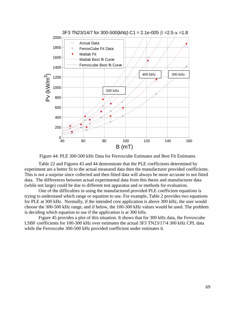
Figure 40: CPL graph using MATLAB Method............................................................... 65 Figure 41: PLE LSBF for the 100-300 (kHz) data ........................................................... 66 Figure 42: PLE LSBF for the 300-500 (kHz) data ........................................................... 67 Figure 43: PLE 100-300 kHz Data for Ferroxcube Estimates and Best Fit Estimates ..... 68 Figure 44: PLE 300-500 kHz Data for Ferroxcube Estimates and Best Fit Estimates ..... 69 Figure 45: 100-300 and 300-500 kHz 3F3 Ferroxcube equations vs 300 kHz data ......... 70
iv
Figure 46: 100-500 BFLS for Hysteresis Loss Equation .................................................. 71
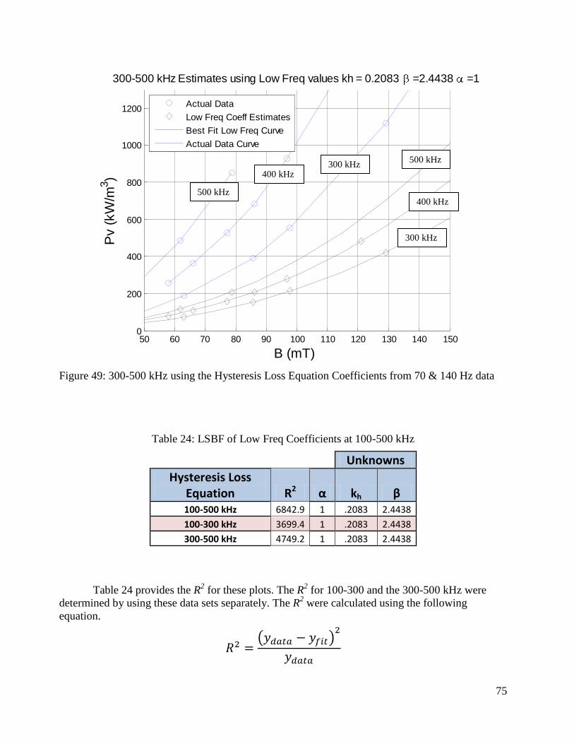
Figure 47: 100-500 kHz Using the HLE Coefficients from 70 & 140 Hz data ................ 73 Figure 48: 100-300 kHz using the HLE Coefficients from 70 & 140 Hz data ................. 74 Figure 49: 300-500 kHz using the HLE Coefficients from 70 & 140 Hz data ................. 75
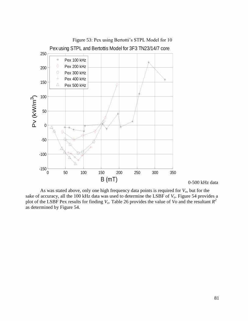
Figure 50: CECE for 100-500 kHz Data........................................................................... 77 Figure 51: Bertotti’s STPL Model Using 100 kHz Data .................................................. 79 Figure 52: Bertotti’s STPL Model Using 500 kHz Data .................................................. 80 Figure 53: Pex using Bertotti’s STPL Model for 100-500 kHz data ................................ 81 Figure 54: Bertotti’s Excess Eddy Loss LSBF Vo term using 100 kHz data ................... 82
Figure 55: Bertotti's Model vs Actual data for 100-500 kHz ........................................... 83 Figure 56: Plot of Bertotti's Model minus the Excess Loss Term .................................... 85 Figure 57: HLE & PLE Model Plot .................................................................................. 86
List of Tables Table 1: Ferroxcube 3F3 Constants [12] .......................................................................... 10
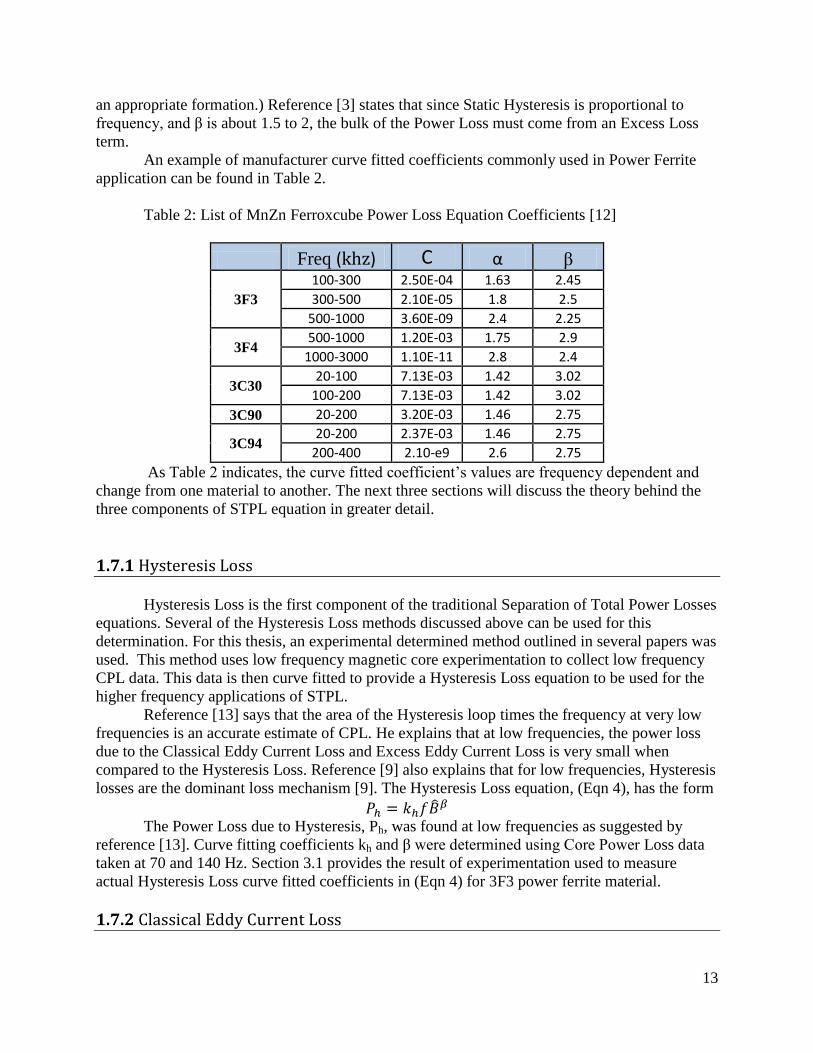
Table 2: List of MnZn Ferroxcube Power Loss Equation Coefficients [12] .................... 13 Table 3: Matrix and MATLAB Validation Table ............................................................ 36
Table 4: Results of the MATLAB and Matrix Method ................................................... 37 Table 5: Residuals of Hysteresis Equation at 70 Hertz..................................................... 41 Table 6: Using the BFLS 70 hertz coefficients for 140 hertz estimates ........................... 42
Table 7: BFSL 70 and 140 Hertz data for Hysteresis Loss Equation (α=1) ..................... 43 Table 8: BFSL 70 and 140 Hertz data for Hysteresis Loss Equation (α unconstrained) .. 44
Table 9: Effective Core Area of Cores used ..................................................................... 53 Table 10: Error for same lot same size cores .................................................................... 54 Table 11: 100 kHz Region 1 Core Loss Core Comparison .............................................. 56
Table 12: 100 kHz Region 2 Core Loss Core Comparison .............................................. 57 Table 13: 500 kHz Region 1 Core Loss Core Comparison .............................................. 59
Table 14: 500 kHz Region 2 Core Loss Core Comparison .............................................. 59 Table 15: 500 kHz Region 3 Core Loss Core Comparison .............................................. 59
Table 18: R2 and LSBF Steinmetz Equation coefficients at High Freq ............................ 63
Table 19: Residuals for High Freq using the Power Law Equation ................................. 65
Table 20: Residual data for 100-300 (kHz) PLE .............................................................. 66 Table 21: Residual data for 300-500 (kHz) PLE .............................................................. 67 Table 22: Residuals of PLE for both Manufacturer Data and Estimated ......................... 68 Table 23: The Hysteresis Loss Equation LSBF for 100-300 kHz and 300-500 kHz ....... 72 Table 24: LSBF of Low Freq Coefficients at 100-500 kHz ............................................. 75
Table 25: Residuals for Classical Eddy Current Equation................................................ 77 Table 26: EECL LSBF Residuals in finding Vo by using 100 kHz data at 100 kHz Pex .. 82
Table 27: R2 for Bertotti's Model minus the Excess Loss Term ....................................... 84
Table 28: HLE & PLE Model LSBF Results.................................................................... 86 Table 29: LSBF R
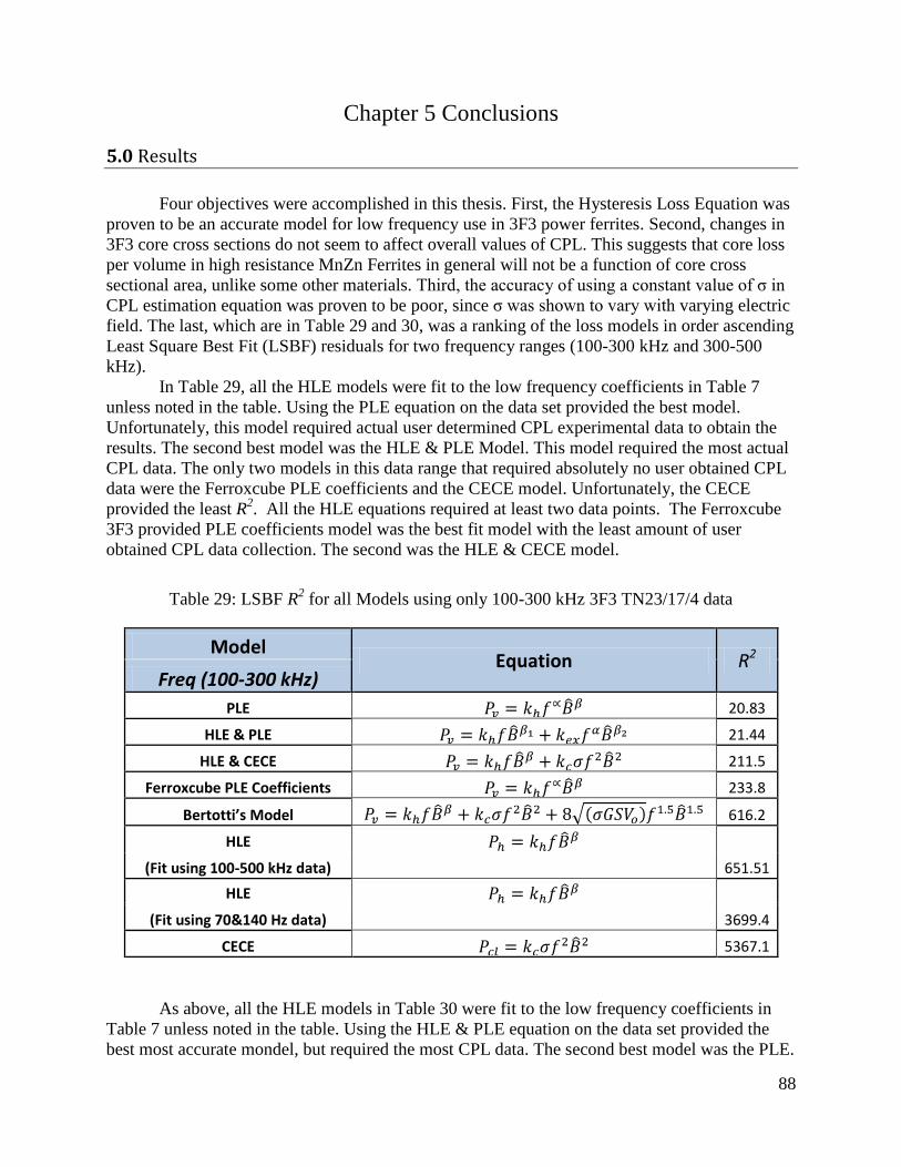
2 for all Models using only 100-300 kHz 3F3 TN23/17/4 data ........... 88
Table 30: LSBF R2 for all Models using only 300-500 kHz 3F3 TN23/17/4 data ........... 89
Table 31: TN23/14/7 Data 70 Hz, 140 Hz and 100 kHz data ......................................... 105 Table 32 TN23/14/7 Data 200 - 500 kHz data ................................................................ 106
v
Table 33: Conductivity AC data for 3F3 Plata ............................................................... 107
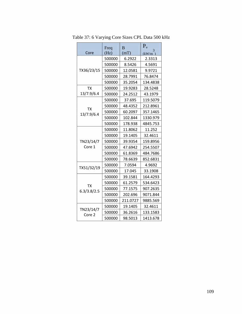
Table 34: DC Conductivity for 3F3 Plate ....................................................................... 107 Table 35: Data using Impedance Analyzer ..................................................................... 108 Table 36: 6 Varying Core Sizes CPL Data 100 kHz ...................................................... 108
As explained in Section 2.4, conductivity, σ, performs an important role in many
empirical equations and models. An example of this can be found in (Eqn 6), the Classical Eddy
Current Equation (CECE), for cylindrical cores and sine-wave excitation.
Since many Separation of Total Power (STPL) models include the CECE, a good
estimate of σ used in the CECE is important to get an accurate CPL estimate. A list of the terms
in the CECE can be found in section 1.5. In several places in the literature ([5] and [26]), σ is
said to be only temperature and frequency dependent, but an experiment conducted by reference
[24] indicates that σ in power ferrites might also be electric field dependent. TheHis high electric
field and frequency experimentations there produced very non-linear σ values. Reference [24]
supposed that the possible combination of high frequencies and large electric fields produced a
phenomenon called charge tunneling. See reference [24] for an in-depth explanation of this
postulated charge tunneling phenomenon. His conclusion was that σ was AC electric field
dependent.
To validate [24] results, a test fixture similar to [24] fixture was built. Figure 9 is a
schematic drawing of this apparatus. A description of the apparatus and the mathematics
involved in calculating σ are found in Section 2.5.
Figure 24: Conductivity Apparatus (Note: It was noted afterwards that there is the potential for
dc grounding issues with this connection, but the RF measurements appeared reasonable.)
46
Varying 100 and 500 kHz sinusoidal voltages at two temperatures, 44°C and 64°C, were
used in the experiment. Figure 25 is a plot of the results using σ and Electric Field as axes. σ is
given by the following equation and Electric field is the voltage peak across the plate, Vo,
divided by the length of the plate.
As explained in Section 2.4, is the length of the material, A is the cross sectional area of
the material that the current flows through and R is the resistance of the structure.
Figure 25 demonstrates that for a 3F3 Power Ferrite material and sine wave excitation,
plate σ is clearly frequency dependent with a slight temperature dependency. This supported the
above [5] and [26] assertions. Figure 25 also corroborates reference [24] conclusion that σ in
power ferrite materials has electric field dependencies, since σ increased with rises in electric
field strength. If σ was independent of electric field values, σ would have remained constant for
increases in electric field strength.
0
0.5
1
1.5
2
2.5
3
3.5
200 400 600 800 1000 1200 1400 1600 1800
Co
nd
uct
ivit
y (1
/Ω-m
)
Electric Field (Volt/m)
AC Conductivity vs Electric Field
63C at 500khtz
44C at 500khtz
63C at 100khtz
47
Figure 25: AC Conductivity vs varying AC Electric Field
If σ changes with changes in peak electric field strength as demonstrated by Figure 25,
one can easily infer that σ also changes during the voltage fluctuations in every sine-wave half
cycle. This would make CPL empirical equations models like CECE, which typically use
constant DC σ values in their empirical estimation equations, both invalid and not accurate CPL
estimation methods.
Reference [24] demonstrated that σ varied during a condition of both high AC
frequencies and large electric fields. So, DC σ experiments were performed to see if similar σ
variations would still be present. It was interesting to see that comparable results occurred.
Figure 26: DC Conductivity vs Electric Field
0
0.05
0.1
0.15
0.2
0.25
0.3
0.35
0 500 1000 1500 2000 2500 3000 3500 4000
Co
nd
uct
ivit
y (1
/Ω-m
)
Electric Field (Volt/m)
DC Conductivity vs Electric Field
44C
55C
63C
48
The same apparatus was used, with the exception that the signal generator and amplifier
were replaced with a DC amplifier. As seen in the AC σ experiment and in Figure 26,
temperature affects complex σ values. It was also surprising that large DC electric fields also had
variations of complex σ.
The results demonstrated in Figure 25 and 26 contradict several papers which explains
that conductivity has a relatively constant value for varying electric fields. As the above figures
show, the value of σ can fluctuate more than double to triple its lowest σ value depending upon
the value of the electric field. This means CPL empirical equations that use σ, similar to the
CECE, could also fluctuate 2 to 3 times depending upon which DC σ value was used in that
equation.
Section 2.4 gives three methods typically used to obtain the σ value used in many CPL
empirical equations:
1. to measure DC σ at a specified temperature, either 25 C or the temperature of the
power ferrite intended application,
2. to measure AC σ at the same frequency and temperature used in the desired power
ferrite application, and
3. to use the manufacturer’s provide DC σ value. This value is usually measured at
25 C.
The most likely accurate method to obtain σ is to find a method that determines σ with
the most similar parameters as the one used in the power ferrite application. The further away
from inteded use parameters, the more likely error will be present in the estimation.
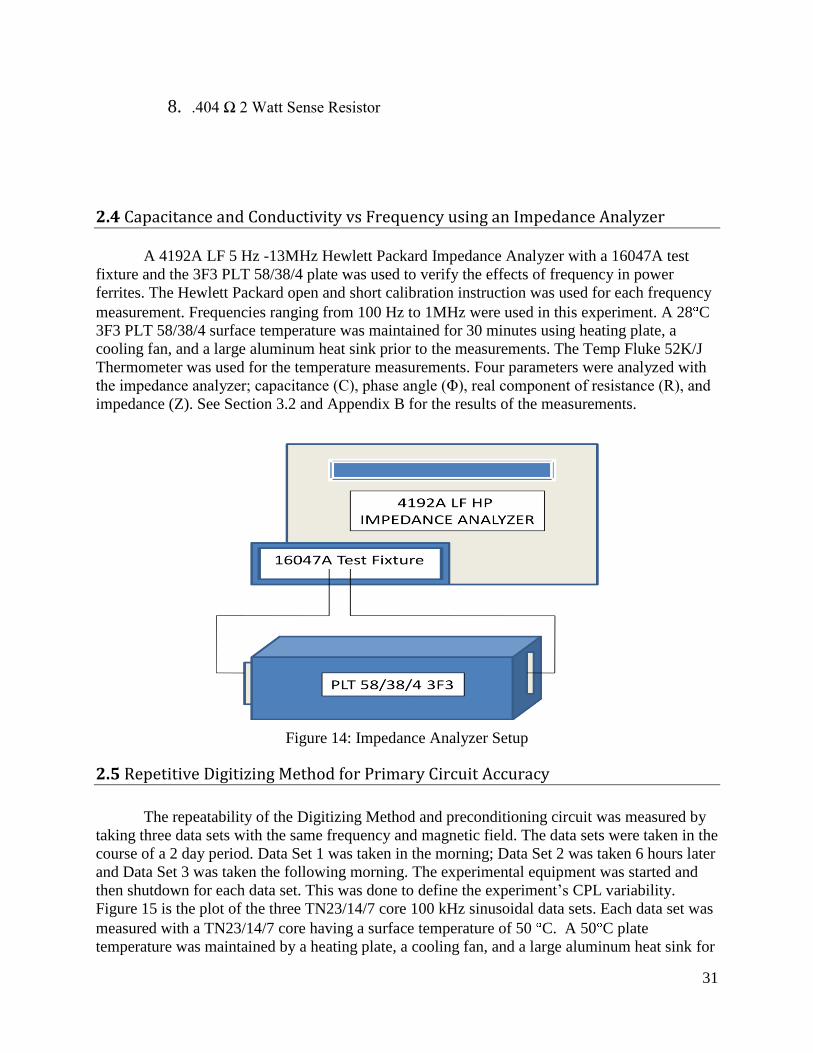
The last experiment conducted to measure σ was performed using 4192A LF 5 Hz -
13MHz Hewlett Packard Impedance Analyzer with a 16047A test fixture on the 3F3 plate
material. This experiment was conducted to analyze a surprising result found making the AC σ
measurement using the 3F3 PLT 58/38/4 material.
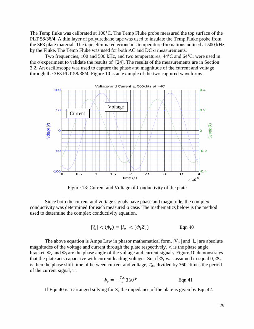
As noticeable in Figure 27, which is an oscilloscope snap shot of the voltage and current
through the 3F3 PLT 58/38/4 plate, the plate has a large capacitive value. As Figure 27
demonstrates the current leads voltage. What makes this fascinating is that most Power Ferrites
are used as inductors. A possible reason to account the plate have a capacitive value might be
due to the fact the 3F3 plate is made of Manganese Zinc, (MnZn). MnZn has a crystalline
structure which is insulated by an isolating layer that creates pockets of MnZn throughout the
material [26]. Ferroxcube, the manufacturer of 3F3, gives the size of MnZn grain between 10um
to 20um. [26] The boundary between the grains is estimated to about ½ that value. The small
pockets of ferrite material act like small capacitive plates separated by electrolytic boundary
layers.
49
Figure 27: Voltage and Current of the 3F3 PLT 48/38/4 σ measurements
The frequencies used in this experiment ranged from 100 Hz to 1 MHz. The Surface
temperature of the 3F3 PLT 58/38/4 plate was maintained at 28 C. Four parameters were
measured from the impedance analyzer; capacitance (C), phase angle (Φ), real component of
resistance (R), and impedance (Z). See section 7 for a table of the results.
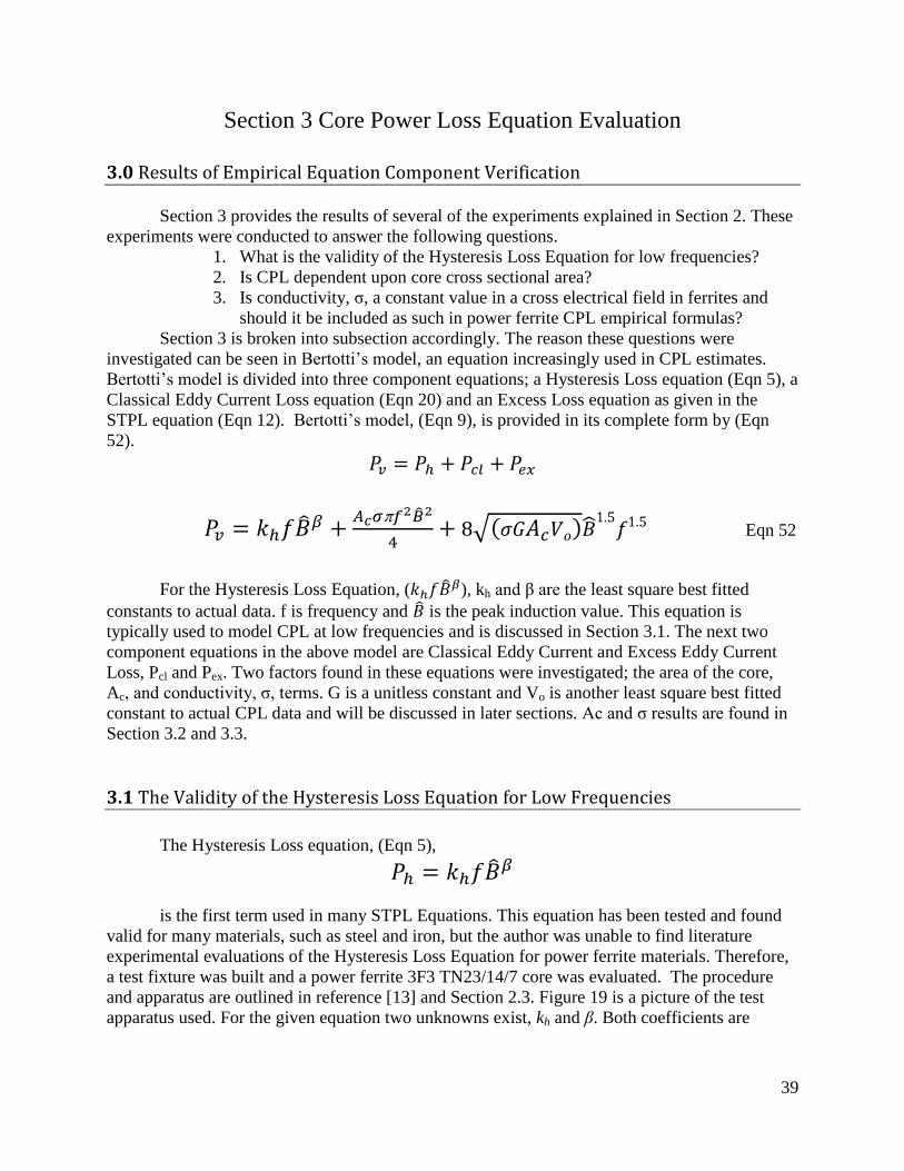
Figure 28 is a graph of capacitance versus frequency.
0 0.5 1 1.5 2 2.5 3 3.5 4
x 10-6
-100
-50
0
50
100
Vol
tage
(V)
Voltage and Current at 500khtz at 44C
time (s)
0 0.5 1 1.5 2 2.5 3 3.5 4
x 10-6
-0.4
-0.2
0
0.2
0.4
Cur
rent
(A)
50
Figure 28: 3F3 Plate Capacitance vs Freq
Figure 29 is the phase versus frequency. At 100 hHz the measured phase angle between
current and voltage for the 3F3 TN23/14/7 core was 57 °. This correlates well with the 62.4° impedance phase angle measured at 100 kHz by the impedance analyzer.
1.E-10
1.E-09
1.E-08
1.E-07
1.E-06
1.E-05
1.E-04
100 1,000 10,000 100,000 1,000,000
Cap
acit
ance
(F)
Freq (Hz)
Capacitance vs Freq
51
Figure 29: Phase Angle vs Freq
Figure 30: Resistance vs Freq for 3F3 Plate Measurement
3.3 Core Area as a factor in CPL per volume Equations
As emphasized in Section 2.0, there are many CPL empirical equations that use cross-
sectional core area, (AC), as an empirical estimation equation factor. For example, Bertotti’s
model uses Ac for two if its component equations, the Classical Eddy Current Loss and Excess
Power Loss equations, as demonstrated in Eqn 52.
-80
-70
-60
-50
-40
-30
-20
-10
0
10
10 100 1000 10000 100000 1000000
Ph
ase
An
gel (
°)
Freq (Hz)
Phase Angle Vs Freq
0
2
4
6
8
10
12
14
16
10 100 1,000 10,000 100,000 1,000,000
Res
itan
ce (
kΩ)
Freq (Hz)
Resistance Vs Freq
52
One goal of this research thesis was to determine if CPL per volume is dependent upon
core area for power ferrites. Numerous experimental literature exists on this topic for a wide
range of materials, but very little was found using power ferrite materials.
In this experiment, six 3F3 toroid cores were analyzed with AC ranging from 3 to 186
mm2. An in-depth explanation of the test procedure and the CPL test apparatus used for this
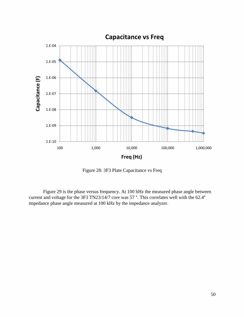
experiment is located in Section 2.1. AC for a perfect rectangular cross-section toroid would be
the multiplication of the height of the core (h) and width of the ferrite material (w). Fig 5 is an
example of the these dimensions used in AC calculations.
Figure 31: Rectangular Toroid Figure
Unfortunately, the cores used in the experiment were not perfect rectangular toroids. The
manufacturer rounds the edges of the core using a tumbler. To account for difference due to
rounded edges, the effective area (Ae) provided by Ferroxcube’s data sheets were used to
determine the given AC (Ferroxcube is the manufacturer of the 3F3 cores).
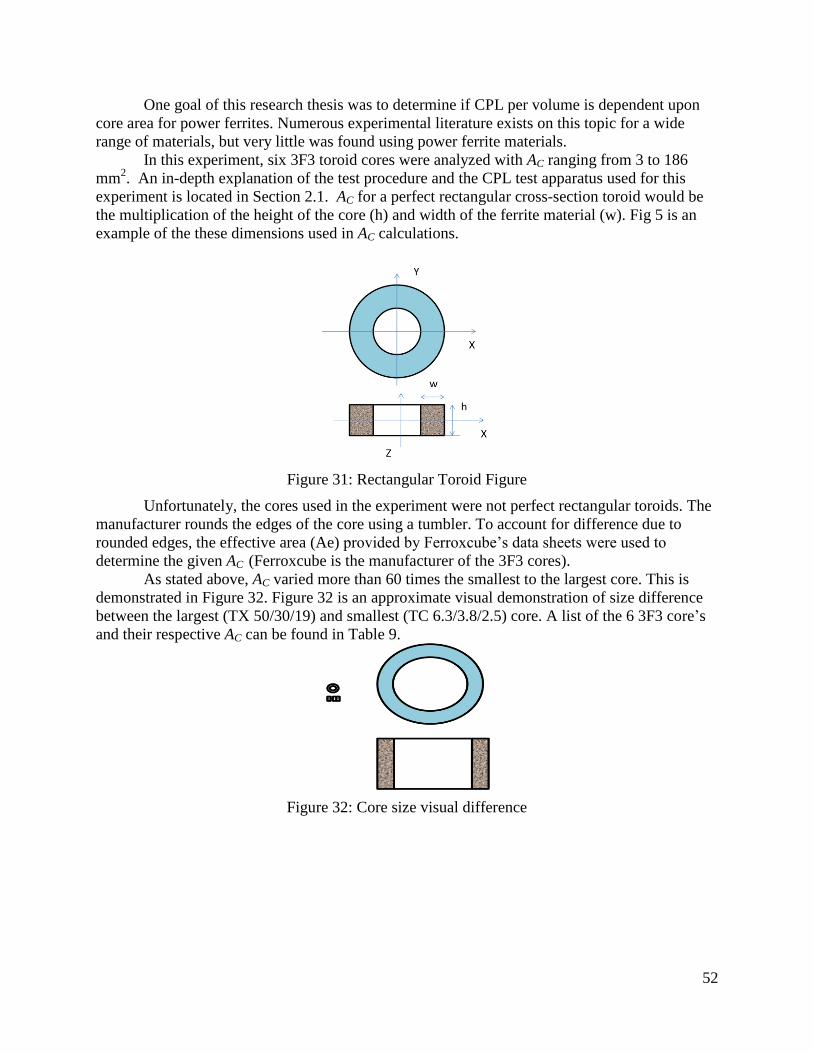
As stated above, AC varied more than 60 times the smallest to the largest core. This is
demonstrated in Figure 32. Figure 32 is an approximate visual demonstration of size difference
between the largest (TX 50/30/19) and smallest (TC 6.3/3.8/2.5) core. A list of the 6 3F3 core’s
and their respective AC can be found in Table 9.
Figure 32: Core size visual difference
53
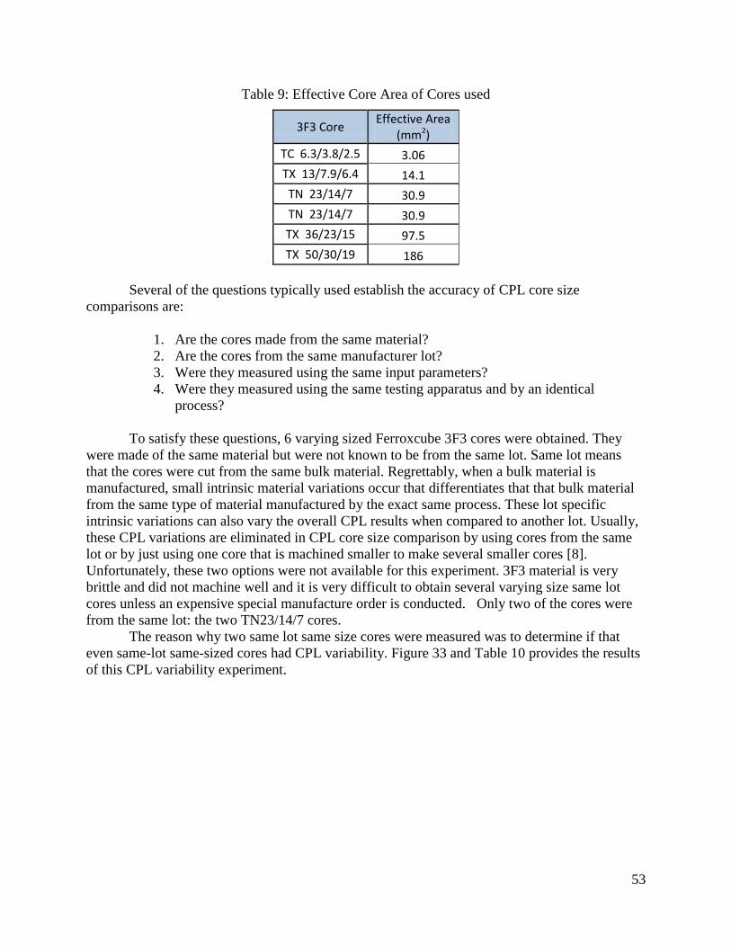
Table 9: Effective Core Area of Cores used
3F3 Core Effective Area
(mm2)
TC 6.3/3.8/2.5 3.06
TX 13/7.9/6.4 14.1
TN 23/14/7 30.9
TN 23/14/7 30.9
TX 36/23/15 97.5
TX 50/30/19 186
Several of the questions typically used establish the accuracy of CPL core size
comparisons are:
1. Are the cores made from the same material?
2. Are the cores from the same manufacturer lot?
3. Were they measured using the same input parameters?
4. Were they measured using the same testing apparatus and by an identical
process?
To satisfy these questions, 6 varying sized Ferroxcube 3F3 cores were obtained. They
were made of the same material but were not known to be from the same lot. Same lot means
that the cores were cut from the same bulk material. Regrettably, when a bulk material is
manufactured, small intrinsic material variations occur that differentiates that that bulk material
from the same type of material manufactured by the exact same process. These lot specific
intrinsic variations can also vary the overall CPL results when compared to another lot. Usually,
these CPL variations are eliminated in CPL core size comparison by using cores from the same
lot or by just using one core that is machined smaller to make several smaller cores [8].
Unfortunately, these two options were not available for this experiment. 3F3 material is very
brittle and did not machine well and it is very difficult to obtain several varying size same lot
cores unless an expensive special manufacture order is conducted. Only two of the cores were
from the same lot: the two TN23/14/7 cores.
The reason why two same lot same size cores were measured was to determine if that
even same-lot same-sized cores had CPL variability. Figure 33 and Table 10 provides the results
of this CPL variability experiment.
54
Figure 33: 3F3 TN 23/14/7 same size core lot Variability
Table 10 provides the average maximum error between the two same lot TN 23/14/7
cores for the same overlapping 100 and 500 kHz regions.
Table 10: Error for same lot same size cores
Frequency (kHz)
Average Error
Max Error
100 6.90% 13.40%
500 1.40% 3.78%
Since, the average error determined at 100 kHz between the same lot cores was 6.9% and
the Section 2.5 average error between same size different lot core data sets was 6.54%, this
experiment demonstrates the same lot cores might have greater variation then different lot cores.
As explained above, to minimize the potential errors that arise from comparing CPL from
different lots, five different sized cores from unique lots cores were used. By using multiple lots
and sizes, the overall chances of lot variability on one particular lot from affecting the general
overall core size CPL trends is minimized.
Figure 34 is a plot of the 6 cores for both 100 and 500 kHz frequency data sets. The most
interesting result of Figure 34 is there does not seem to be a clear trend in the data. The smallest
core, TC6.3/3.8/2.5, actually had the highest loss. This is surprising if Bertotti’s model (Eqn 52)
5
50
500
Pv
(kW
/m3
)
B (mT)
Same Size Core Core Power Loss vs Magnetic Field
TN23/14/7-Ae (30.9)
TN23/14/7-Ae (30.9)
55
is correct. The expected lowest CPL core using Eqn 52 would be the core with the smallest area,
since AC is found twice in the equation with terms proportional to Ac and Ac1/2
.
Figure 34: Core Area effects on Core Loss
Figure 35 provides the CPL loss data of Figure 34’s for just 100 kHz. One of the
TN23/14/7 cores was removed to provide a clearer picture of the trends. The removal of this core
did not change the data trends. The graph was then is broken into overlapping curve regions.
Only overlapping actual experimental data points were compared in the experiment to eliminate
the potential error that experimental estimates could give.
Region 1 in Figure 35 envelops 4 cores and Region 2 encases 3. Table 11 and 12 are the
rankings of the cores in each region from smallest to largest AC and their respective ranking of
their Total CPL from lowest to highest (Ranking was ordered by figure trends, so the core with
Lowest CPL trend had CPL rank of 1). Contrary to Classical Eddy Current Loss theory, for
Region 1 the largest CPL loss was the smallest core and the second lowest loss core was the
largest core. For Region 2 of Figure 35, the medium sized AC had the lowest CPL.
Table 11: 100 kHz Region 1 Core Loss Core Comparison
100 (khz)
Core
AC
(mm2) Lowest
CPL
Region 1
TC6.3/3.8/2.5 3.06 4
TX13/7.9/6.4 14.1 1
TN23/23/7 30.9 3
TX36/23/15 97.5 2
1
10
100
1000
10 60 110 160 210
Pv
(kW
/m3
)
B (mT)
Pv vs B at 100 kHz
TC6.3/3.8/2.5-Ae (3.06)
TX13/7.9/6.4-Ae (14.1)
TN23/14/7-Ae (30.9)
TX36/23/15-Ae (97.5)
TX50/30/19-Ae (186)
Region 1
Region 2
100 kHz
57
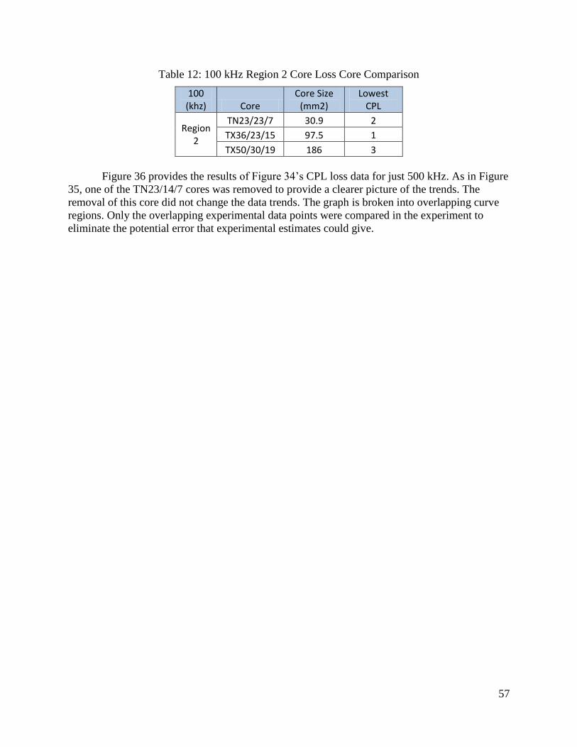
Table 12: 100 kHz Region 2 Core Loss Core Comparison
100 (khz) Core
Core Size (mm2)
Lowest CPL
Region 2
TN23/23/7 30.9 2
TX36/23/15 97.5 1
TX50/30/19 186 3
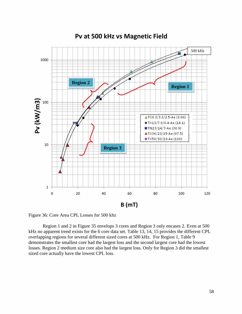
Figure 36 provides the results of Figure 34’s CPL loss data for just 500 kHz. As in Figure
35, one of the TN23/14/7 cores was removed to provide a clearer picture of the trends. The
removal of this core did not change the data trends. The graph is broken into overlapping curve
regions. Only the overlapping experimental data points were compared in the experiment to
eliminate the potential error that experimental estimates could give.
58
Figure 36: Core Area CPL Losses for 500 khz
Region 1 and 2 in Figure 35 envelops 3 cores and Region 3 only encases 2. Even at 500
kHz no apparent trend exists for the 6 core data set. Table 13, 14, 15 provides the different CPL
overlapping regions for several different sized cores at 500 kHz. For Region 1, Table 9
demonstrates the smallest core had the largest loss and the second largest core had the lowest
losses. Region 2 medium size core also had the largest loss. Only for Region 3 did the smallest
sized core actually have the lowest CPL loss.
1
10
100
1000
0 20 40 60 80 100 120
Pv
(kW
/m3
)
B (mT)
Pv at 500 kHz vs Magnetic Field
Region 3
Region 2 Region 1
500 kHz
59
Table 13: 500 kHz Region 1 Core Loss Core Comparison
500 (khz) Core
Core Size (mm2)
Lowest CPL
Region 1
TC6.3/3.8/2.5 3.06 3
TX13/7.9/6.4 14.1 1
TN23/23/7 30.9 2
Table 14: 500 kHz Region 2 Core Loss Core Comparison
500 (khz) Core
Core Size (mm2)
Lowest CPL
Region 2
TX13/7.9/6.4 14.1 1
TN23/23/7 30.9 3
TX36/23/15 97.5 2
Table 15: 500 kHz Region 3 Core Loss Core Comparison
500 (khz) Core
Core Size (mm2)
Lowest CPL
Region 3
TX36/23/15 97.5 1
TX50/30/19 186 2
The conclusion that can be drawn from the data of figures 35 and 36 is that CPL is
independent of AC , or at least that AC is not a dominant factor in CPL calculations for 3F3 power
ferrite material. What needs to be emphasized is that if core area were a significant consideration
then loss per volume would have varied greatly among the cores, since there is a factor of 60
area variation between the cores.
Three articles were found that discussed Power Ferrite core area versus CPL. Two of the
references supported this author’s claim that core area might not be a dominant CPL factor in
Power Ferrites([5] and [8]), and one contradicted it [17].
The author of [5] explains that when a material is divided into small insulated electrical
grain regions, the CPL per volume is more affected by the size of the grain and insulation layer
around that grain then the overall dimension of the ferrite core. He further explains that for
ferrite materials with high amplitude magnetic loss, the CPL per volume is independent of ferrite
core dimension [5].
The above statement, about independence of loss per volume from core size, was
experimentally verified by the authors of [8]. Their experiment systematically decreased the size
of two MnZn ferrite cores through machining. The difference between the two cores was the
amount of insulator in the cores. The first core, with little insulator, had low resistivity and a high
value of permeability. Both properties are not typically found in high frequency applications [8].
In contrast, the second core, with more insulator, had ideal high frequency properties: high
resistivity and low permeability. The experiment was conducted at two frequencies, 100 and 200
kHz. Table 16 provides these values. The experimental results demonstrated that CPL of the core
60
with little insulator was dependent upon core dimension, while the CPL of the more insulator
core was not. This result supports that insulation layer thickness has an effect on CPL values.
The authors of [17] conducted CPL measurements using two different sized, but same
MnZn material, power ferrite cores. The lot of the cores was not mentioned. Their core intrinsic
material of choice also had a high resistivity and a low permeability, both ideal power ferrite
application materials [8]. Table 16 provides these values. The cores were measured using 10 to
1000 kHz. Their conclusion did not agree with those of [8]. For their data set, there seemed to be
a correlation of core size and CPL for cores with the same characteristics of the second core used
in [8]. Their conclusion is that a portion of Power Ferrites CPL is due to the displacement of
current distributions in the core. Different shaped and size cores would change this distribution
[17].
Table 16 demonstrates that the cores chosen in this thesis resemble both the second core
used in [8] and both cores used in [27]. The results of this thesis did not show a trend in core size
to CPL, which was supported by [5] and [8]. The difference in the testing of the cores, might be a
factor in the differing results of the between this thesis, [8] and [17].
Table 16: Core Resistivity and Permeability values
Core used in experiment @DC
(Ωm) r
[8] MnZn First Core (Little insulator) 0.15 10000
[8] MnZn Second Core (More insulator) 6.5 2300
[Thesis] MnZn 3F3 Ferrite Core 8 3000
[17] MnZn Both Cores 10 3080
61
Section 4 CPL Data Fitting and Statistics Analysis
Section 4 provides the Least Square Best Fit (LSBF) statistical analysis for the CPL
estimation equations listed in Section 1.6. As stated in Section 2.7, two mathematic LSBF methods
were used for this analysis, a matrix and a MATLAB non-linear fit. Section 4 is broken into
subsections, one for each equation. Each subsection includes the matrix math used to obtain both
the LSBF curve fitted coefficients and the LSBF residuals value. The MATLAB code used to
calculate the coefficients and LSBF residuals (R2) in each of the following subsections can be
found in Appendix B. For each equation, the curve fitted coefficients of the lowest LSBF residual
method were used in the plot of the equation. The method, the procedure and CPL measuring
apparatus used to obtain the CPL data set used for the LSBF, is located in Section 2.3. The R2 were
calculated using Eqn 45.
As stated in Section 2.7, R2 is the Least Square Best Fit Residuals value. ydata is the actual
measured CPL data. yfit is results of using LSBF coefficient data.
4.1 Steinmetz Equation
Steinmetz proposed an equation in 1892 for the loss of energy due to hysteresis loss for
machine steel. The equation had the form [7]. is the power loss per unit volume, is
the maximum peak flux amplitude, β and k are curve-fitted coefficients of actual experimental
data. For Steinmetz’s applications, this equation was a good solution for estimating CPL.
Unfortunately, this equation is not robust enough to account for the CPL dependent frequency
component. Power Ferrites are typically used frequencies in the range of 100 kHz to a few MHz,
while Steinmetz experimentation used only low frequency sine wave data (50-200 hertz) for his k
and β coefficients estimate [7].
To use Steinmetz Equation, the user has two options. The user can either find the k and β
coefficients by obtaining them through the manufacturer’s data sheet, if available, or measure these
coefficients through actual experiment.
The accuracy of Steinmetz Equation is only as accurate as the data set used to obtain these
coefficients. For example, the R2 are extremely low, i.e. accurate, for the LSBF curve fit to actual
CPL data taken at 70 Hz or 140 Hz, but not when the combined data set of 70 and 140 Hz is used
for the LSBF. Table 17 provides these R2 values.
Table 17: Steinmetz Equation
Unknowns
Steinmetz Equation R2 k β
Low Freq (70 & 140) Matrix .059 18.89 2.38
Low Freq (70) MATLAB .00006 19.68 2.67
Low Freq (140) MATLAB .00098 22.77 2.24
62
Figure 37 is a plot of actual 70 Hertz CPL data and the LSBF curve fitted solution to that
data.
Figure 37: Hysteresis Loss Equation for 70 Hertz
The differences between R2 between the 70 Hz data and the 70 and 140 Hz combined data
is due to Steinmetz equation (not accounting for the frequency dependency of CPL measurements).
Figure 38 is a plot of the LSBF solution to the combined 70 and 140 Hz CPL data set.
Figure 38: Low Frequency Core Power Loss for TN 23/14/7
0 50 100 150 200 250 3000
0.1
0.2
0.3
0.4
0.5
0.6
0.7
0.8
B (mT)
Pv (
kW
/m3)
3F3 TN23/14/7 for 70(htz) kh = 19.5086 =2.6727
Actual Data
Matrix Fit
Matlab Fit
Best fit Curve
0 50 100 150 200 250 3000
0.2
0.4
0.6
0.8
1
1.2
1.4
B (mT)
Pv (
kW
/m3)
3F3 TN23/14/7 for 100-500(khtz) kh = 18.8876 =2.3803
Actual Data
Matrix Fit
Matlab Fit
Best fit Curve 140 Hz
70 Hz
70 Hz
63
The star dotted line is the LBFS solution to the actual CPL data at 70 and 140 hertz. Due to
the input data sets having two different frequencies, the Steinmetz equation splits the difference
between the two. As Table 17 demonstrates, the Steinmetz equation can only accurately
approximate CPL if the frequency of the data set used to obtain the coefficients are the same as the
frequency of the intended estimate.
Figure 39 is the Steinmetz Equation BFLS solution to the 3F3 TN23/17/4 100-500 kHz
data set. As was shown in Figure 38, Steinmetz Equation still provided only a single line solution
to the data set.
Figure 39: High Freq (100-500kHz) Steinmetz Equation
The LSBF R2 for the TN23/14/7 core for the 100 to 500 kHz data set is in Table 18.
Table 18: R2 and LSBF Steinmetz Equation coefficients at High Freq
Unknowns
Steinmetz Equation R2 k β
High Freq (100- 500) 1956.5 5909.19 1.0587
The Matrix method was evaluated using the following equations. Using logarithms the
Steinmetz Equation can be broken down into the form y= C+Dx. This is a linear equation, which
40 60 80 100 120 140 160 180 2000
500
1000
1500
B (mT)
Pv (
kW
/m3)
3F3 TN23/14/7 for 100-500(khtz) kh = 5909.1876 =1.0587
Actual Data
Matrix Fit
100 khz
200 khz 300 khz
400 khz
500 khz
64
can be easily evaluated using LSBF matrix mathematics. The matrix math used in this CPL
equation can found in reference [27].
The matrix equivalent form of the above equation follows.
= b
See Appendix B for the program used to calculate the MATLAB non linear solution.
4.2 Power Law Equation (PLE)
As shown in Section 1.6 and 4.1, for an equation to accurately estimate Power Ferrite CPLs
over a broad range, that equation needs to have both a frequency and magnetic field term. The
Power Law Equation is one such equation. Currently, the Power Law Equation (PLE) is of
standard equation used by manufacturers, scientist and engineers. The simplicity of this approach
is the parameters required for the equation can be found in manufacturer’s material data sheets.
Unlike several of the other empirical equations, this equation does not require the user to collect
experimental data. Note that this equation does not account for possible variations in loss density,
with core cross-sectional area.
The PLE (Eqn 5) has the following form:
is the power loss per unit volume, is the maximum peak flux amplitude, f is the
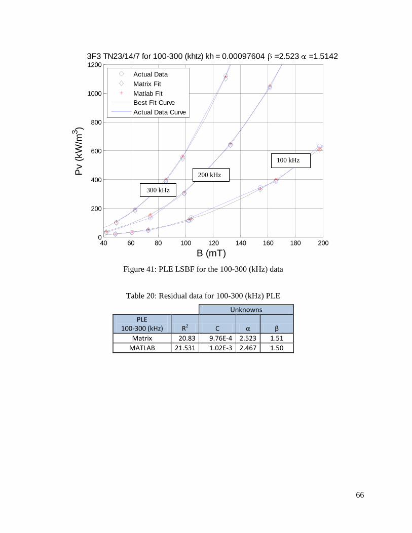
frequency, and α, β and C1 are curve-fitted coefficients of actual experimental data. The 3F3 TN23/14/7 100-500 kHz data set was used to determine the PLE accuracy when
compared to actual CPL core data. Figure 40 provides the LSBF curve fitted coefficients, C1, α and
β, for the PLE.
65
Figure 40: CPL graph using MATLAB Method
Table 19 gives the R2 for both Matrix and MATLAB method. For this equation, the
MATLAB method provided the lowest LSBF R2 values.
Table 19: Residuals for High Freq using the Power Law Equation
%%%%%%%%% Put back in t=linspace(0,length(V1)*tint,length(V1)); %Creates a time function for the %%%%%%%%%%% V1=detrend(V1,'constant');
%gives the index of the Voltages to find what is a waveform [Vzero, Zerot, Zerotact] = Zero(V1, t); %Shows the Zero pionts of the gragh
n=0; while rem(length(Zerot)-1-n,2)==0 %used to give only a full cycle of Voltage n=n+1; %if odd number of zeros windows in end min1=1; %first zero crossing used later on if length(Zerot)==3 max1=2; else %first zero crossing used later on max1=length(Zerot)-n-2; %As n goes up the max value of zeros
goes down end %As n goes up the max value of zeros goes down
V1=Vtemp; I1temp=I1(Zerot(1):Zerot(3)); Imean=mean(I1temp); for i=1:length(V1) Itemp(i)=I1(i)-Imean; end
I1=Itemp; %Gives the Power of I1 and V1 for q=1:length(V1) P(q)=I1(q)*V1(q); end %gives the index of the Voltages to find what is a waveform % [Vzero, Zerot, Zerotact] = Zero(V1, t); %Shows the Zero pionts of the
gragh % n=0; % while rem(length(Zerot)-1-n,2)==0 %used to give only a full cycle of
Voltage % n=n+1; %if odd number of zeros windows in % end % min1=1; %first zero crossing used later on % max1=length(Zerot)-n %As n goes up the max value of zeros
goes down z=1; %temp iterator i=1; y=1; o=1; while i~=(max1)/2+1 %uses a while loop, seemed to work better then for
loop do not know why for m=(Zerot(y)):(Zerot(y+2)) %iterates over the range of one
voltage cycle Bflux(z)=tint*trapz(V1((Zerot(y)):m))/(N*Ae); %Starts at zero and
then gets Bflux if m~=Zerot(y+2) %for the cycle z=z+1; end end p=z; %sets the limit on one half cycle Bpeak(i)=(max(Bflux(o:p))-min(Bflux(o:p)))/2; %gives the Bpeak of
every cycle i=i+1; %iterates the while loop y=y+2; %iteratates the wave o=z; %sets the limit on one half cycle end
if mean(Bflux)<=0 %% Ensures the B vs H leans to the right by flipping the
B values and making them positive Bflux=Bflux.*(-1); end
95
Vtemp=V1(Zerot(min1):(Zerot(max1+1))); %Vtemp is used in the plot over the
range of Bflux Btime=t(Zerot(min1):(Zerot(max1+1))); %Btime is used in the
plot of time the range of Bflux Bpk=mean(Bpeak)*1000; %Gives the Bpeak
of the waveforms Bmin=min(Bflux); Bmax=max(Bflux);
%%%%%%%%%% %%Gives the H field using N,Reff, and I as input parameters for q=1:length(I1) Hfield(q)=I1(q)*N/le; end y=1; i=1; %Gives the Pk of the H while i~=(max1)/2+1 Hpeak(i)=(max(Hfield(Zerot(y):Zerot(y+2)))-
min(Hfield(Zerot(y):Zerot(y+2))))/2; i=i+1; y=y+2; end Hpk=mean(Hpeak);
%%%%%%%%%%%%%%%%%%%%%%%%%%%%%%%%% %Pvavg z=1; %increments Paveout i=1; %Breaks while loop q=1; %Increments time average of P y=1; u=1;
%%%%%%%%%%%%%%%%%%%%%%%%%%%%%%%%%%%%%%%%%%%%%%%%%%%%%% for hysterisis %%%%%%%%%%%%%%%%%%%%%%%%%%%%%%%%%%%%%%%%%%%%%%%%%%%%%% test % Vecm=1 %Ve=Vecm/10^6 %%%%%%%%%%%%%%%%%%%%%%%%%%%%%%% while i~=(max1)/2+1 for m=(Zerot(y)):(Zerot(y+2)) if m-Zerot(y)==0 Paveout(z)=0; z=z+1; else Paveout(z)=tint*trapz(P(Zerot(y):m))*(1000/Vecm)/(tint*(m-
mhorel, mhospec ) % fprintf('\n') % % figure(1) % plotVandI(t,V1,I1,tint,Bpk) %Plots the data of V and Current % %title('Voltage') % figure(1) % %hold on %
if Hmax_in < Hmin_in first_in=Hmax_in; sec_in=Hmin_in; else first_in=Hmin_in; sec_in=Hmax_in; end Bused=detrend(Bused, 'constant'); third_in=first_in+Hlength; sumtrap=-(trapz(Hused(first_in:sec_in),Bused(first_in:sec_in))+
trapz(Hused(sec_in:third_in),Bused(sec_in:third_in))); Pvhys=(sumtrap/(tint*length(Zerot(1):Zerot(3))))*10^-3; % figure(4) % grid on % hold on % plot(Hused(first_in:sec_in),Bused(first_in:sec_in),'b') % plot(Hused(sec_in:third_in),Bused(sec_in:third_in),'r') Bmax=max(Bused)*1000;
%The below is the MATLAB code used to determine the Least Square Best Fit
%Residuals for the PLE equation and provide a plot of the data. All other
%models used this code with slight modifications. This program calls the
%LSQRmat file and a Pvdata dat file. Both codes will follow this program.
This %code was written by Colin Dunlop
clc; clear;
[X,y]=Pvdata(); name=@PLE_func; [beta0,yfit]=LSQRmat; %The coefficient results are the matrix fit are fed
into
%fed into a array for plotting
yfitmatrix=feval(name,beta0,X);
options = statset('TolFun',1e-40,'TolX',1e-
40,'MaxIter',160000,'DerivStep',1e-10); [beta,R,J]= nlinfit(X,y,name,beta0); %nlinfit is a built in Matlab function ci = nlparci(beta,R,J); %which provides the non linear fit to
data [Ypred, delta] = nlpredci(name,X,beta,R,J); x=X(:,2);
%%%%%%%%%%%%%%%%%%%%%%%%%%%%%%%%%%%%%%%% yfit=feval(name,beta,X); for i=1:length(x) chi(i)=(((y(i)-yfit(i))).^2)/y(i); end
RChiSquare = sum(chi);
% %%%%%%%%%%%%%%%%%%%%%%%%%%%%%%%%%% % %%% PLOTTING YOUR DATA AND FIT %%% % %%%%%%%%%%%%%%%%%%%%%%%%%%%%%%%%%% % figure (1); % opens figure 1 and makes it active clf; % clears the active figure hold on; % Makes matlab plot without clearing the graph
%plot(x,y,'k*') %plot(x,y,'rx'); % Plots the fitted curve hold on; % Makes matlab plot without clearing the graph
plot(x,y,'bo') plot(x,yfitmatrix,'kd'); % Plots the fitted curve plot(x,Ypred,'r.'); % Plots the fitted curve array=(linspace(30,300,20))'; D=300000.*ones(length(array),1); %creates a ones array the length of the
% array=(linspace(30,300,20))'; % D=300000.*ones(length(array),1); %creates a ones array the length of the
number of B inputs % % A=cat(2,D,array); % yfitcurve=feval(name,beta,A); % % plot(array,yfitcurve,'r--'); % % array=(linspace(30,300,20))'; % D=400000.*ones(length(array),1); %creates a ones array the length of the
number of B inputs % % A=cat(2,D,array); % yfitcurve=feval(name,beta,A); % % plot(array,yfitcurve,'r--'); % array=(linspace(30,300,20))'; % D=500000.*ones(length(array),1); %creates a ones array the length of the
number of B inputs % % A=cat(2,D,array); % yfitcurve=feval(name,beta,A); % % plot(array,yfitcurve,'r--');
x1=min(x); x2=max(x); grid on % axis([40,340,0,2250]);
101
%axis([x1-1/16*x1,x2,min(y),max(y)]); % sets visible range of the plot % % title(['3F3 TN23/14/7 for 100-300(khtz) kh = ',num2str(beta0(1,1)),' \beta
=',num2str(beta0(2,1)),' \alpha =',num2str(beta0(3,1))],'fontsize',12); % % % Places the title on the graph %xlabel('B (mT)','fontsize',14,text(5,120,['\chi^2_\nu-1 = ' str1]) ); %