Modeling of 3D Magnetostrictive Systems with Application to Galfenol and Terfenol-D Transducers Dissertation Presented in Partial Fulfillment of the Requirements for the Degree Doctor of Philosophy in the Graduate School of The Ohio State University By Suryarghya Chakrabarti, B.S. Graduate Program in Mechanical Engineering The Ohio State University 2011 Dissertation Committee: Marcelo Dapino, Advisor Rajendra Singh Ahmet Kahraman Junmin Wang
Transcript
Modeling of 3D Magnetostrictive Systems with Application to
Galfenol and Terfenol-D Transducers
Dissertation
Presented in Partial Fulfillment of the Requirements for the DegreeDoctor of Philosophy in the Graduate School of The Ohio State
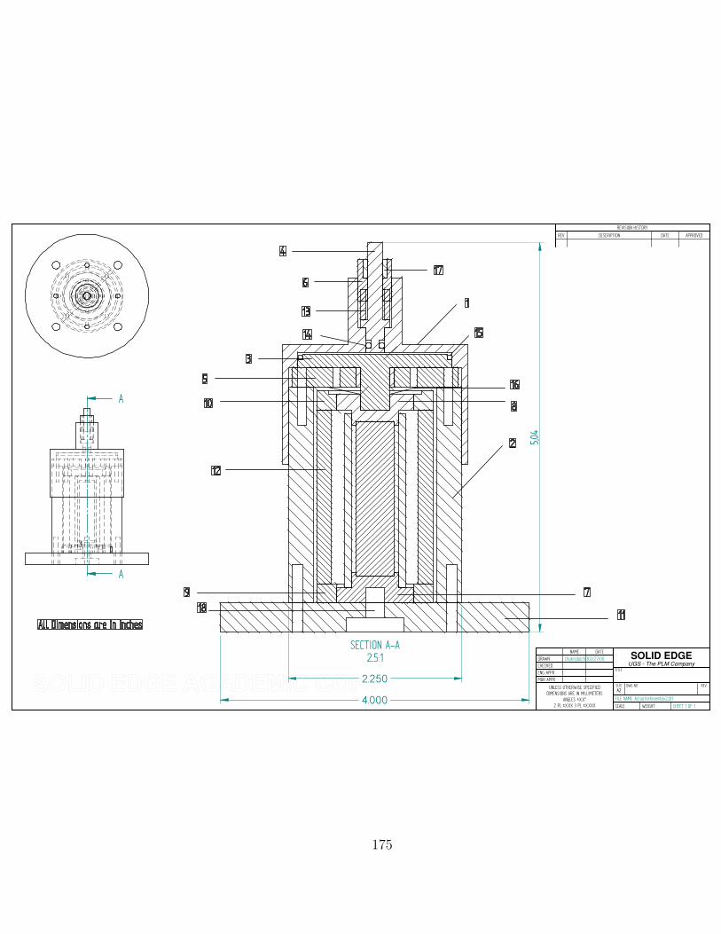
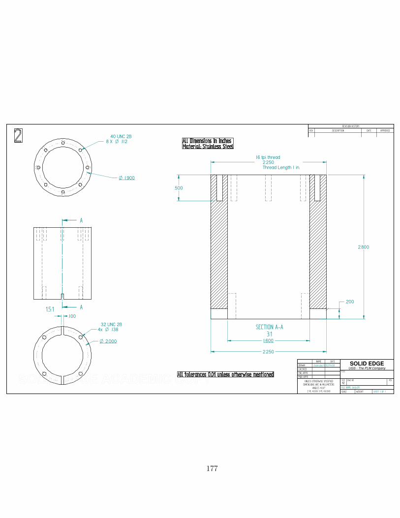
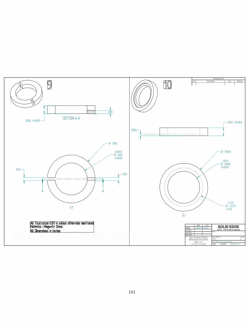
S. Chakrabarti and M.J. Dapino, “A dynamic model for a displacement amplifiedmagnetostrictive driver for active mounts,” Smart Materials and Structures, Vol. 19,pp. 055009, 2010.
S. Chakrabarti and M.J. Dapino, “ Nonlinear finite element model for 3D Galfenolsystems,” Smart Materials and Structures, Vol. 20, pp. 105034, 2011.
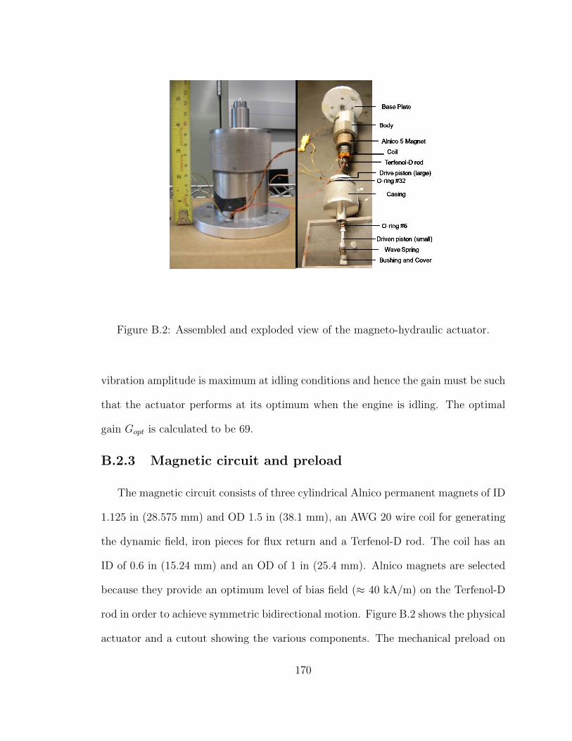
S. Chakrabarti and M.J. Dapino, “Hydraulically amplified Terfenol-D actuator foradaptive powertrain mounts,” ASME Journal of Vibration and Accoustics, (acceptedfor publication)
S. Chakrabarti, M.J. Dapino, “Hydraulically amplified magnetostrictive actuator foractive engine mounts,” in Proceedings of the ASME conference on Smart MaterialsAdaptive Structures and Intelligent Systems, Vol. 1, pp. 795-802, October 2008.
S. Chakrabarti, M.J. Dapino, “Design and modeling of a hydraulically amplifiedmagnetostrictive actuator for automotive engine mounts,” in Proceedings of SPIE,Vol. 7290, April 2009.
viii
S. Chakrabarti, M.J. Dapino, “Modeling of a displacement amplified magnetostric-tive actuator for active mounts,” in Proceedings of the ASME conference on SmartMaterials Adaptive Structures and Intelligent Systems, Vol. 2, pp. 325-334, October2009.
S. Chakrabarti, M.J. Dapino, “Design and modeling of a hydraulically amplifiedmagnetostrictive actuator for automotive engine mounts,” in Proceedings of SPIE,Vol. 7645, April 2010.
S. Chakrabarti, M.J. Dapino, “Coupled axisymmetric finite element model of amagneto-hydraulic actuator for active engine mounts,” in Proceedings of SPIE, Vol.7979, April 2011.
S. Chakrabarti, M.J. Dapino, “3D dynamic finite element model for magnetostrictiveGalfenol-based devices,” in Proceedings of SPIE, Vol. 7978, April 2011.
Fields of Study
Major Field: Mechanical Engineering
Studies in:
Smart Materials and StructuresFinite element methodElectromagnetismNonlinear dynamics
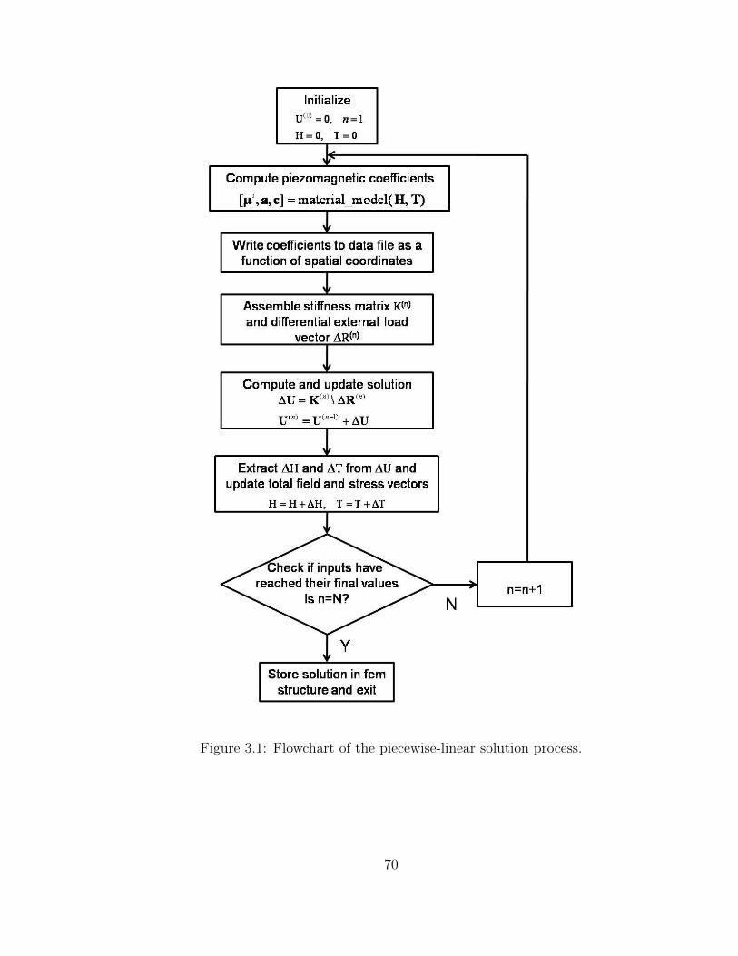
3.1 Flowchart of the piecewise-linear solution process. . . . . . . . . . . . 70
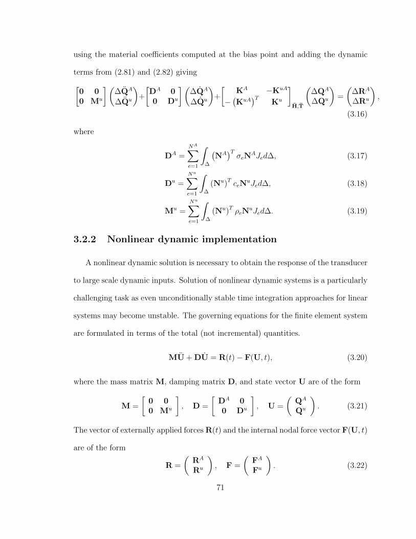
3.2 Outline of a single time step of the nonlinear dynamic solution algo-rithm. The flowchart shows how quantities at time t+∆t are obtainedwith knowledge about all variables at time t. . . . . . . . . . . . . . . 75
3.3 Screenshot of the global expressions relating flux density and strain tothe vector magnetic potential and displacements. . . . . . . . . . . . 76
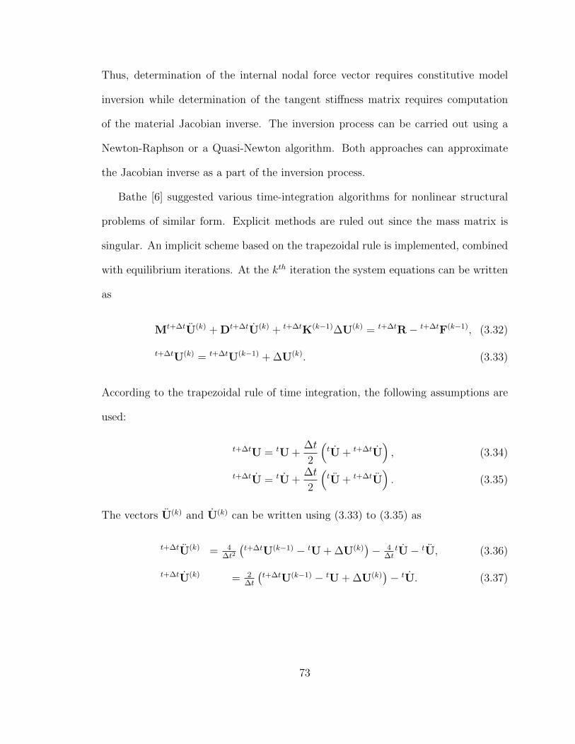
3.5 Screenshots of the weak and time-dependent weak terms (dweak) forthe magnetic subdomain. . . . . . . . . . . . . . . . . . . . . . . . . . 78
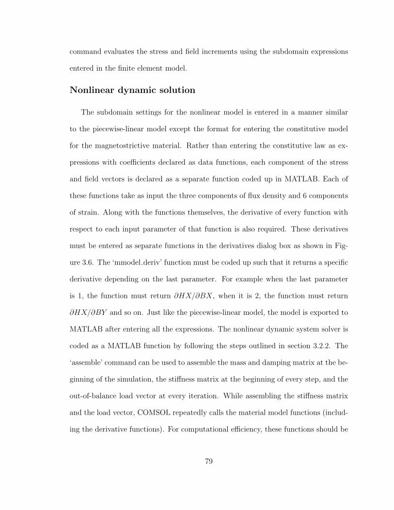
3.6 Screenshot showing the function definition for HX and declaration ofthe derivative functions. . . . . . . . . . . . . . . . . . . . . . . . . . 80
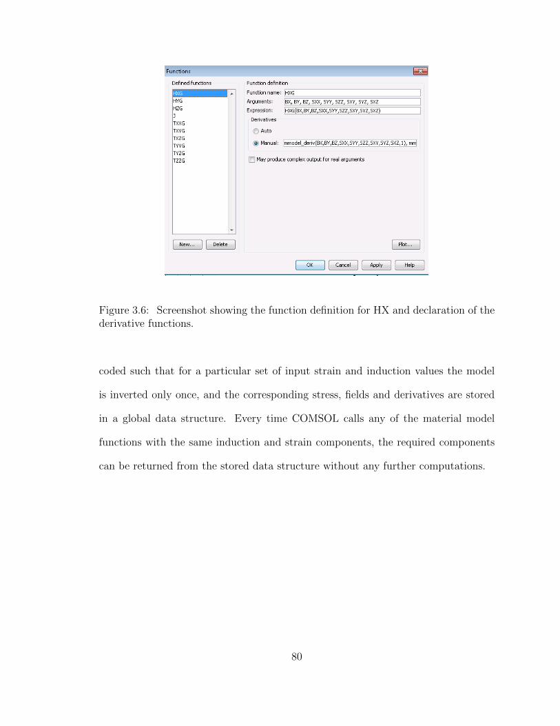
4.1 A schematic representation for the solution of a 3D finite element modelshowing how a parameter optimization algorithm can eliminate theneed for complex 3D measurements and subsequent interpolation. . . 85
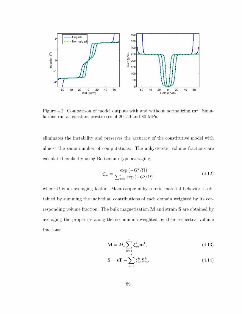
4.2 Comparison of model outputs with and without normalizing mk. Sim-ulations run at constant prestresses of 20, 50 and 80 MPa. . . . . . . 89
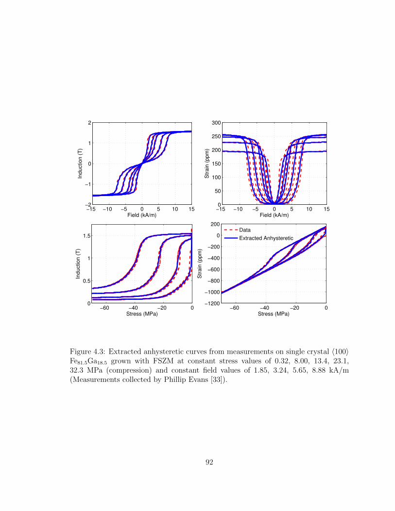
4.3 Extracted anhysteretic curves from measurements on single crystal〈100〉 Fe81.5Ga18.5 grown with FSZM at constant stress values of 0.32,8.00, 13.4, 23.1, 32.3 MPa (compression) and constant field valuesof 1.85, 3.24, 5.65, 8.88 kA/m (Measurements collected by PhillipEvans [33]). . . . . . . . . . . . . . . . . . . . . . . . . . . . . . . . . 92
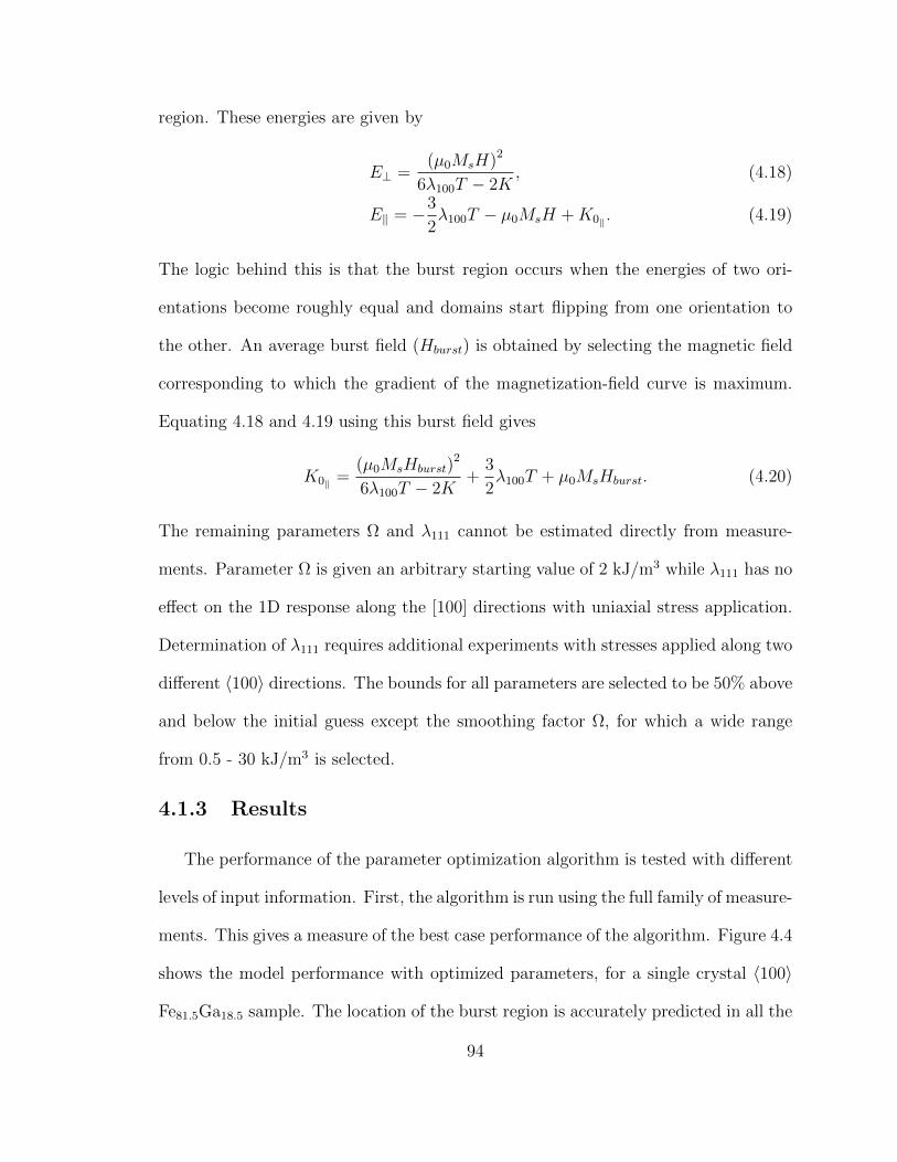
4.4 Comparison of anhysteretic model to the extracted anhysteretic curvesfrom measurements on a Fe81.5Ga18.5 sample. Actuation measurementsare at constant compressive stresses of 0.32, 8, 13.4, 23.1, and 32.3MPa while sensing measurements are at constant bias fields of 1.85,3.24, 5.65, and 8.88 kA/m. . . . . . . . . . . . . . . . . . . . . . . . . 95
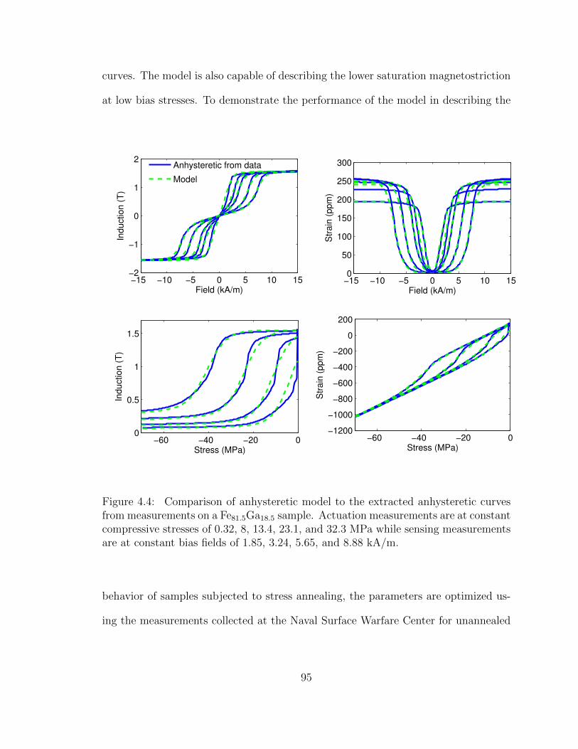
4.5 Anhysteretic model fit to the extracted anhysteretic curves with opti-mized parameters for unannealed 〈100〉 textured polycrystalline Fe81.6Ga18.4.Measurements are at constant compressive pre-stresses of 1.38 , 13.8,27.6, 41.4, 55.2, 69.0, 82.7, and 96.5 MPa. . . . . . . . . . . . . . . . 96
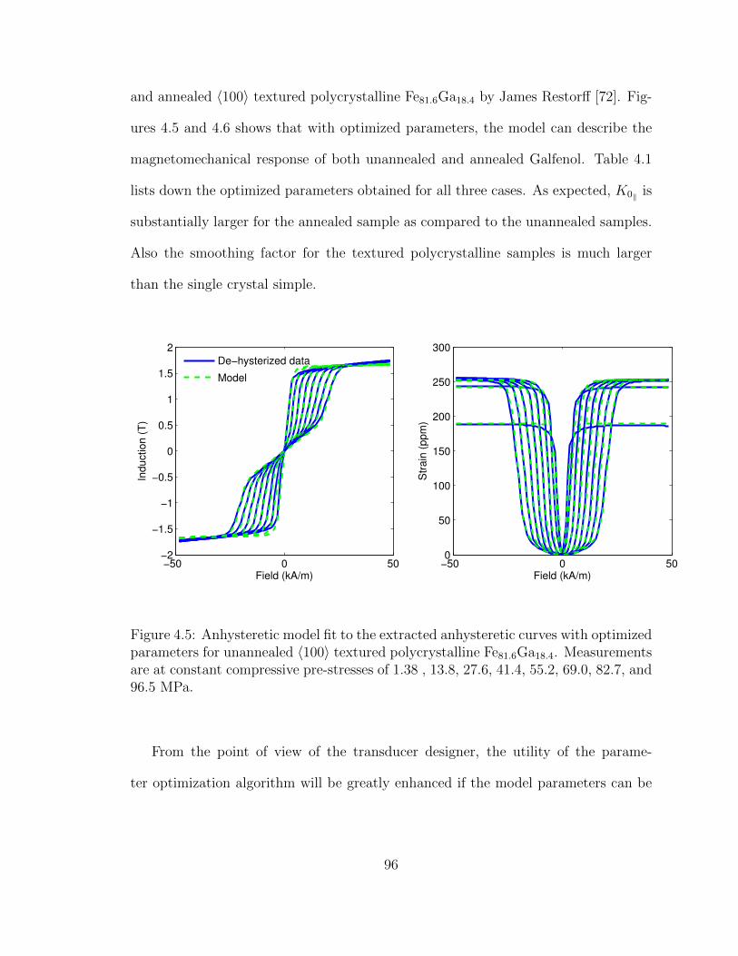
4.6 Anhysteretic model fit to the extracted anhysteretic curves with opti-mized parameters for annealed 〈100〉 textured polycrystalline Fe81.6Ga18.4.Measurements are at constant compressive pre-stresses of 1.38 , 13.8,27.6, 41.4, 55.2, 69.0, 82.7, and 96.5 MPa. . . . . . . . . . . . . . . . 97
4.7 Galfenol unimorph actuator used for model validation, (a) actuatorconfiguration, and (b) finite element mesh. . . . . . . . . . . . . . . . 103
4.8 Quasistatic model results, (a) voltage-deflection, (b) voltage-current. . 104
4.14 Actuator response to harmonic excitation at 10 Hz. . . . . . . . . . . 109
4.15 Actuator response to harmonic excitation at 50 Hz. . . . . . . . . . . 109
4.16 Actuator response to harmonic excitation at 100 Hz. . . . . . . . . . 109
4.17 Actuator response to harmonic excitation at 200 Hz. . . . . . . . . . 110
5.1 Comparison of magnetization and magnetostriction curves for Terfenol-D at 13.5 MPa compressive stress [31] with the Armstrong model [2]and the Discrete Energy Averaged Model (DEAM) [32]. . . . . . . . . 114
5.2 Armstrong model [2] and DEAM [32] with high smoothing factors for13.5 and 41.3 MPa prestress. The higher prestress curve shows thereappearance of kinks in both models. . . . . . . . . . . . . . . . . . . 115
5.3 Armstrong model [2] and DEAM [32] with low smoothing factors show-ing the magnitude of the two kinks with increasing stress. . . . . . . . 116
5.4 (a) Ω-field and (b) strain-field curves for compressive prestresses of 0,6.5, 13.5, 27.4, 41.3, and 55.3 MPa. . . . . . . . . . . . . . . . . . . . 121
5.6 Flowchart for the anhysteretic model. Details of the energy minimiza-tion is shown in section 4.1.1. . . . . . . . . . . . . . . . . . . . . . . 124
5.7 Comparison of the two modeling approaches with actuation data [62]for compressive prestresses of 6.9, 15.3, 23.6, 32.0, 40.4, 48.7, 57.1, and65.4 MPa. . . . . . . . . . . . . . . . . . . . . . . . . . . . . . . . . . 125
5.8 Performance of the two modeling approaches in predicting the stress-strain behavior of Terfenol-D [62] for bias field values of 11.9, 31.8,55.7, 79.3, 103, 127, 151, and 175 kA/m with parameters estimatedfrom the strain-field curves. . . . . . . . . . . . . . . . . . . . . . . . 126
5.9 Comparison of the two modeling approaches with sensing data from[51] for bias magnetic fields of 16.1, 48.3, 80.5, 112.7, 144.9, and 193.2kA/m. . . . . . . . . . . . . . . . . . . . . . . . . . . . . . . . . . . . 126
5.10 Comparison of hysteretic model with data from Moffett et al [62] forcompressive prestresses of 6.9, 15.3, 23.6, 32.0, 40.4, 48.7, 57.1, and65.4 MPa. Parameters optimized for actuation curves. . . . . . . . . . 130
5.11 Comparison of hysteretic model with sensing data from Kellogg etal [62] for bias magnetic fields of 16.1, 48.3, 80.5, 112.7, 144.9, and193.2 kA/m. . . . . . . . . . . . . . . . . . . . . . . . . . . . . . . . . 130
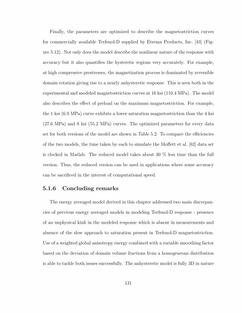
5.12 Comparison of hysteretic model with magnetostriction measurementsprovided by Etrema Products Inc. [43] for compressive prestresses of1, 4, 8, and 16 KSI (6.9, 27.6, 55.2, 110.4 MPa). . . . . . . . . . . . . 133
5.13 Flowchart showing the process followed to incorporate the Terfenol-Dconstitutive law in the model. . . . . . . . . . . . . . . . . . . . . . . 141
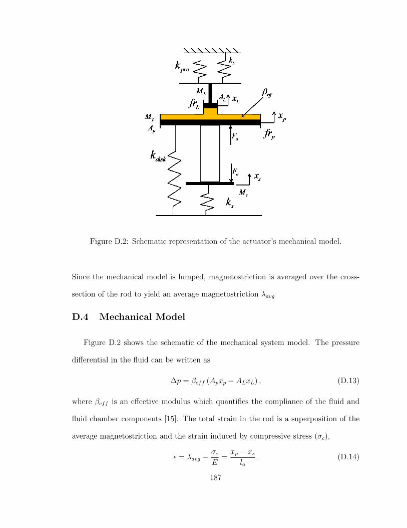
The mass and damping matrix are state-independent and hence are assembled only
once for the entire simulation. The internal nodal force vector F and the tangential
stiffness matrix K are assembled in every iteration as they are state-dependent (Fig-
ure 3.2. Thus, efficient computation of F and K is vital to the performance of the
model.
3.3 Implementation on COMSOL and MATLAB
The modeling framework described in sections 2.4 and 3.2 is implemented on
COMSOL 3.5a utilizing its ability to interact with MATLAB functions. The basic
template for the model is set-up by using two separate weak-form application modes,
one for the mechanical and one for the magnetic degrees of freedom. The variables for
74
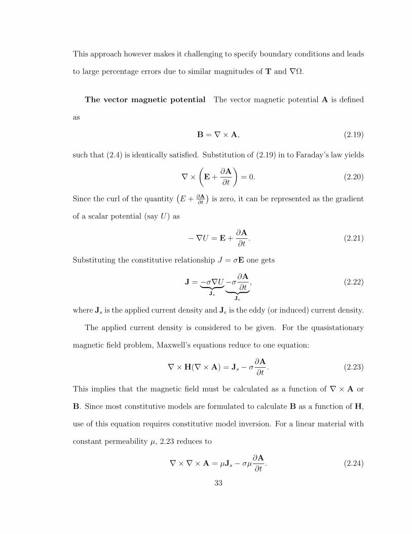
Figure 3.2: Outline of a single time step of the nonlinear dynamic solution algorithm.The flowchart shows how quantities at time t+∆t are obtained with knowledge aboutall variables at time t.
the mechanical mode are uX, uY, uZ while for the magnetic mode are AX,AY,AZ.
This separation of the mechanical and magnetic physics allows for reduction of the
total degrees of freedom in the model. For example, a component which does not
take part in the structural dynamics of the transducer (e.g a coil, air, flux return) is
marked ’inactive’ in the mechanical application mode. This means that the mechan-
ical degrees of freedom are not solved for in these components.
The next step is to add global expressions in the model. These are essentially
kinematic relationships ((2.79) and (2.80)) which are valid irrespective of the mate-
rial (Figure 3.3). The weak form expressions are added in the subdomain settings.
In the domains which are structurally active, the weak terms and time dependent
75
Figure 3.3: Screenshot of the global expressions relating flux density and strain tothe vector magnetic potential and displacements.
expressions are entered as shown in Figure 3.4. Similarly, the weak form expressions
for the magnetically active domains are entered within the subdomain settings of the
magnetic application mode as shown in Figure 3.5. Boundary conditions are entered
within the boundary settings dialog box of each application mode. The set-up of the
model up till here is common for both the piecewise-linear and the nonlinear imple-
mentation. However, the next steps are specific to the solution process being used.
76
(a) (b)
Figure 3.4: Screenshots of the weak and time-dependent weak terms (dweak) for themechanical subdomain.
Piecewise-linear solution
For the piecewise linear solution, the constitutive laws are entered through sub-
domain expressions. Consider a magnetostrictive material whose piezomagnetic coef-
cal properties in addition to exhibiting moderate magnetostriction. These properties
make Galfenol uniquely well-suited for integration within three-dimensional (3D) ac-
tive structures. Galfenol can be used in sensors or actuators capable of withstanding
tension, compression, and shock loads. This chapter deals with coupling a nonlinear
energy-averaged constitutive law for Galfenol with the finite element framework de-
scribed in Chapter 3 to describe the full nonlinear coupling between the electrical,
magnetic, and mechanical domains in Galfenol systems.
A parameter optimization algorithm is proposed to determine the parameters of
the discrete energy averaged model incorporated into the 3D dynamic finite element
framework. The algorithm uses the 1D magnetomechanical actuation and sensing
curves for the Galfenol alloy as input and computes the model parameters by min-
imizing an error functional defined between the modeled curves and measurements.
Initial guesses on the parameters are obtained by using analytical relationships which
relate specific model parameters to certain features in the experimental data. Pa-
rameters are optimized for unannealed single crystal 〈100〉 Fe81.6Ga18.4 and textured
polycrystalline 〈100〉 Fe81.5Ga18.5 alloys with and without stress annealing. A case
82
study on a Galfenol unimorph actuator reveals the ability of the model to describe
the quasistatic and dynamic response of the actuator.
4.1 Parameter estimation of a discrete energy-averaged modelfrom 1D measurements
Implementation of nonlinear coupled constitutive behavior poses a significant chal-
lenge in distributed parameter modeling frameworks. Earlier works modeled magne-
tostrictive behavior using polynomial fits to measurements. For example, Benbouzid
et al. [8] fit surface splines to experimental data while Kannan and Dasgupta [50] used
constitutive relations in an incremental form with coefficients obtained from bi-cubic
spline fits to measurements. Kim et al. [55] used 6th order polynomials to fit the
strain-field behavior of Terfenol-D with a different set of polynomial coefficients for
each preload condition. The use of spline functions to fit measurements has the advan-
tages of easy differentiability and implementation. However, the procedure becomes
rather complex if complete 3D material behavior is required. This would require 3D
measurements to be performed, and bulky splines with 9 components (3 for field and
6 for stress) to be fitted to those measurements. Graham et al. [40] implemented
Galfenol constitutive behavior through look up tables generated a priori using the
Armstrong model [3] for a large number of induction and stress values. Although the
Armstrong model is capable of describing 3D Galfenol behavior, look up tables were
generated for 1D induction and stress inputs. As is the case with splines, extension
to a full 3D version will add significant complexity because it will require generation
of bulky tables with nine inputs and nine outputs.
To overcome the complexities associated with 3D measurements and subsequent
multivariate interpolation, significant emphasis is placed on incorporating efficient
83
theoretical constitutive laws within distributed parameter models. A physically mo-
tivated constitutive law takes advantage of symmetries in the material and is capable
of predicting 3D material behavior with reduced order information.
The response of Galfenol varies significantly depending on its composition [23] and
material processing techniques [73]. Changes in composition or processing methods
can be made as required by an application. For example, increasing Gallium concen-
tration from 18.4% to 20.9% reduces the saturation magnetostriction but increases the
stress range over which the material shows a stress dependent susceptibility change
making it more suitable for force sensing applications [59]. Through a process called
stress-annealing [73, 84] a tetragonal anisotropy can be introduced in Galfenol where
the two 〈100〉 easy directions parallel to the direction of magnetic field application
have a higher anisotropy energy than the remaining four orientations perpendicular
to the sample axis. This enables the alloy to exhibit maximum saturation mag-
netostriction without any compressive preload. An algorithm which optimizes the
constitutive model parameters to describe these variations in Galfenol behavior will
greatly improve the applicability of the constitutive law in transducer design.
This work aims at developing a formal procedure to estimate the parameters of
the anhysteretic discrete energy averaged model for Galfenol which is incorporated
into a finite element framework for transducer level modeling [17]. The parameter
optimization algorithm takes as input selected 1D magnetomechanical measurements
and calculates the constitutive model parameters such that the only inputs required by
the finite element model are the system level parameters (permeability, conductivity,
Young’s modulus etc. of passive materials) and the 1D magnetostrictive material
characterization curves (Figure 4.1). Section 4.1.1 discusses the Galfenol constitutive
84
Figure 4.1: A schematic representation for the solution of a 3D finite element modelshowing how a parameter optimization algorithm can eliminate the need for complex3D measurements and subsequent interpolation.
model and the parameters which need to be optimized. Section 4.1.2 highlights the
main steps that are undertaken in the optimization process including techniques to
make initial guesses on each parameter. In section 4.1.3, the performance of the
optimization algorithm is analyzed for single crystal and textured polycrystalline
Galfenol alloys.
4.1.1 Discrete energy-averaged constitutive model
Models based on energy weighted averaging employ statistical mechanics to cal-
culate the bulk magnetization and strain of the material. In continuous form (eg.
Armstrong’s model [3]), this approach involves calculation of macroscopic material
response as an expected value of a large number of possible energy states (or do-
main orientations) with an energy based probability density function. Due to the
85
large computational effort involved in evaluating the expected values by solving two
dimensional integrals numerically, a discrete version of the model was developed [2].
The choice of possible domain orientations was restricted to the easy magnetization
axes with volume fraction of domains in each state calculated using a discretized
version of the probability density function. The increase in computational speed,
however, came at the cost of reduced accuracy. To preserve accuracy without sacri-
ficing efficiency, Evans and Dapino [32] developed a constitutive model for Galfenol
by choosing orientations which minimize an energy functional locally defined in the
vicinity of each easy axis.
The anisotropy energy GkA is formulated about the kth easy axis ck as
GkA =
1
2Kk‖mk − ck‖2, (4.1)
where the constants Kk control the anisotropy energy landscape in the vicinity of the
easy axes. The anisotropy energy along each easy axis is, however, identically zero.
For materials with cubic anisotropy (such as unannealed Galfenol), the anisotropy
energy along each easy axis is the same and the model can be applied in its present
form. However, it has been shown that stress annealing induces tetragonal anisotropy
in Galfenol [73] where the four 〈100〉 directions perpendicular to the annealing direc-
tion have a lower energy than the other two. To make the model capable of describing
these effects, the anisotropy energy is modified as
GkA =
1
2K‖mk − ck‖2 +Kk
0 , (4.2)
where K controls the energy landscape in the vicinity of the easy axes and Kk0 specifies
the base anisotropy energy along the kth easy axis. Six parameters are required to
describe the anisotropy energy (K,K10 , ..., K
50), where Kk
0 is defined as the anisotropy
86
energy relative to the sixth easy axis. Thus, the total number of parameters is same
as the earlier description of anisotropy energy [32]. Further, the m-dependent portion
of the anisotropy energy remains unchanged, which means the minimization results
remain unaffected.
With this definition, the total free energy of a domain close to the kth easy axis
ck is formulated as the sum of the local anisotropy energy GkA, magnetomechanical
coupling energy GkC and the Zeeman energy Gk
Z ;
Gk =1
2K‖mk − ck‖2 +Kk
0︸ ︷︷ ︸Gk
A
−Skm ·T︸ ︷︷ ︸Gk
C
−µ0Msmk ·H︸ ︷︷ ︸
GkZ
, (4.3)
which must be minimized with respect to the orientation vector mk in the vicinity
of ck. The minimization problem is constrained (‖mk‖ = 1) and is formulated as
an inhomogeneous eigenvalue problem through the use of Lagrange multipliers. The
total energy is written as
Gk =1
2mk ·Kmk −mk ·Bk +
1
2K +Kk
0 , (4.4)
where the magnetic stiffness matrix K and force vector Bk are
K =
K − 3λ100T1 −3λ111T4 −3λ111T6
−3λ111T4 K − 3λ100T2 −3λ111T5
−3λ111T6 −3λ111T5 K − 3λ100T3
, (4.5)
Bk =[ck1K + µ0MsH1 ck2K + µ0MsH2 ck3K + µ0MsH2
]T. (4.6)
The Lagrange function is constructed as the sum of the energy functional and unity
norm constraint on the orientation vectors linearized about the easy axis orientations
(mk ·mk = 1 ≈ ck ·mk = 1):
L =1
2mk ·Kmk −mk ·Bk + λk
(ck ·mk − 1
), (4.7)
87
where λk is the Lagrange multiplier corresponding to the kth easy axis. Differentiating
the Lagrange function with respect to mk and equating to zero one gets
mk = K−1[Bk − λkck
]. (4.8)
Substitution of mk from (4.8) into the constraint yields the following expression for
the Lagrange multiplier:
λk = −1− ck · (K)−1 Bk
ck · (K)−1 ck, (4.9)
which on substitution into (4.8) gives the following analytical expression for the ori-
entation which minimizes the energy around the kth easy axis, of the form
mk = (K)−1
[Bk +
1− ck · (K)−1 Bk
ck · (K)−1 ckck
]. (4.10)
A limitation of the constitutive law in its current form is that the unity norm con-
straint on mk is not strictly enforced. As a result at very high fields well in the
saturation regime, the norm of mk can become much greater than unity thus yield-
ing unphysical magnetization and strain calculations (Figure 4.2). This issue can
be addressed by strictly enforcing the unity norm constraint rather than using the
approximation mk · mk = 1 ≈ ck · mk = 1. However, that leads to a sixth order
equation for the Lagrange multiplier requiring numerical techniques for solution thus
compromising the efficiency of the model [32]. In order to maintain the stability of the
model without sacrificing its efficiency, mk is normalized and denoted by the symbol
mk in all future calculations where
mk =mk
‖mk‖. (4.11)
Figure 4.2 shows that the output of the model with and without the normalization
is almost the same till the former becomes unstable. Thus normalizing the minima
88
−60 −40 −20 0 20 40 60
−2
−1
0
1
2
Field (kA/m)
Induction (
T)
−60 −40 −20 0 20 40 600
50
100
150
200
250
300
350
400
Field (kA/m)
Str
ain
(ppm
)
Original
Normalized
Figure 4.2: Comparison of model outputs with and without normalizing mk. Simu-lations run at constant prestresses of 20, 50 and 80 MPa.
eliminates the instability and preserves the accuracy of the constitutive model with
almost the same number of computations. The anhysteretic volume fractions are
calculated explicitly using Boltzmann-type averaging,
ξkan =exp
(−Gk/Ω
)∑rj=1 exp (−Gj/Ω)
, (4.12)
where Ω is an averaging factor. Macroscopic anhysteretic material behavior is ob-
tained by summing the individual contributions of each domain weighted by its cor-
responding volume fraction. The bulk magnetization M and strain S are obtained by
averaging the properties along the six minima weighted by their respective volume
fractions:
M = Ms
r∑k=1
ξkanmk, (4.13)
S = sT +r∑
k=1
ξkanSkm. (4.14)
89
The model parameters are the six anisotropy constants, smoothing factor (Ω), mag-
netostriction constants (λ100, λ111), and the saturation magnetization (Ms). The base
anisotropy constants are split into two groups: K0‖ and K0⊥ . K0‖ is the anisotropy en-
ergy for the two orientations parallel to the axis of the rod while K0⊥ is the anisotropy
constant for the four orientations perpendicular to the axis of the rod. Since we are
interested only in the relative anisotropy energies, any one of them can be chosen to
be zero. In this paper, K0⊥ is chosen to be zero, thus reducing the total number of
unknown parameters to six. For unannealed Galfenol, K0‖ is expected to be almost
equal to K0⊥ which is chosen to be zero, while for annealed Galfenol K0‖ is expected
to be significantly larger than K0⊥ due to the induced tetragonal anisotropy.
4.1.2 Parameter optimization procedure
The parameter optimization process consists of two steps. First, anhysteretic
curves are obtained from hysteretic measurements through a simple averaging proce-
dure. This is necessary because we are interested in optimizing the anhysteretic model
parameters only. Next, a least squares optimization routine is used to minimize the
error between the family of modeled curves and the anhysteretic curves obtained from
measurements.
Extracting the anhysteretic curves from measurements
The de-hysterized curves are obtained by computing an average value from the
upper and lower branches of the hysteresis loops (similar to Benbouzid et al. [8]).
As pointed out by Benbouzid et al. [8], this procedure yields an approximate anhys-
teretic value and may not coincide with experimental anhysteretic curves obtained by
superimposing a decaying AC component of the input (field or stress) about a mean
90
value. Since Galfenol exhibits extremely low hysteresis, the error due to this approx-
imation should be negligible. The anhysteretic curves are obtained by sweeping the
input (field or stress) over the entire applied range at discrete steps and finding an
average value of the response over a range of inputs. For example, the anhysteretic
magnetostriction at a field H0 is computed as
San(H0) = AV G(S(H) : H0 − δH < H < H0 + δH), (4.15)
where δH is a small number compared to the maximum applied field. The value
of δH must be chosen carefully. A large value introduces error due to averaging
over a wider range of fields while a very small δH might result in non-existence of
a data point within that range. By calculating the anhysteretic curves using this
method, the data can be sampled at a much lower rate than which it was collected.
This is useful because the material model function is executed as many times as
the number of points on the extracted anhysteretic curve. Fewer number of data
points imply that the material model would be executed fewer times, speeding up the
overall optimization procedure. Figure 4.3 shows measurements and the extracted
anhysteretic curves for a single crystal 〈100〉 Fe81.5Ga18.5 sample grown with FSZM.
Estimating the model parameters
Parameter optimization is done using the MATLAB function fmincon. This func-
tion needs an initial guess and bounds for each parameter. Further it requires a scalar
error definition which it minimizes. The aim of the optimization process is to find the
model parameters which describe the entire family of curves (consisting of different
data sets: magnetization and strain vs field for actuation and vs stress for sensing).
91
−60 −40 −20 00
0.5
1
1.5
Stress (MPa)
Induction (
T)
−15 −10 −5 0 5 10 150
50
100
150
200
250
300
Field (kA/m)
Str
ain
(ppm
)−15 −10 −5 0 5 10 15−2
−1
0
1
2
Field (kA/m)
Induction (
T)
−60 −40 −20 0−1200
−1000
−800
−600
−400
−200
0
200
Stress (MPa)
Str
ain
(ppm
)
Data
Extracted Anhysteretic
Figure 4.3: Extracted anhysteretic curves from measurements on single crystal 〈100〉Fe81.5Ga18.5 grown with FSZM at constant stress values of 0.32, 8.00, 13.4, 23.1,32.3 MPa (compression) and constant field values of 1.85, 3.24, 5.65, 8.88 kA/m(Measurements collected by Phillip Evans [33]).
92
Thus the error functional must describe an average error for an entire family of curves.
This is done in the following manner.
1. For every curve, the modeling error is quantified using a normalized RMS error
definition. The error for the ith curve in a data set is given as
errori =1
range(Xi)
√∑Ni
j=1(Yij −Xij)2
Ni
, (4.16)
where Yij andXij are the jth component of the ith model vector and the extracted
anhysteretic data vector respectively each containing Ni points, and range(Xi)
is the difference between the upper and lower bound for that curve.
2. A mean error for the entire family is obtained by averaging the normalized RMS
errors for each curve in the family.
Initial guess and bounds on each parameter
The efficiency of the optimization algorithm can be greatly enhanced by providing
a good initial guess on the parameters. Ms and λ100 can be directly obtained from the
saturation magnetization and magnetostriction respectively. The anisotropy constant
K is estimated by calculating the slope of the extracted anhysteretic magnetization-
field curve for a particular stress T at zero field and equating it to the expression for
low field stress dependent susceptibility χ(T ) described by Evans et al. [34], giving
K =µ0M
2s
χ(T )+ 3λ100T. (4.17)
The anisotropy constant K0‖ can be estimated by equating the energies of the orien-
tations perpendicular and parallel to the direction of application of field in the burst
93
region. These energies are given by
E⊥ =(µ0MsH)2
6λ100T − 2K, (4.18)
E‖ = −3
2λ100T − µ0MsH +K0‖ . (4.19)
The logic behind this is that the burst region occurs when the energies of two ori-
entations become roughly equal and domains start flipping from one orientation to
the other. An average burst field (Hburst) is obtained by selecting the magnetic field
corresponding to which the gradient of the magnetization-field curve is maximum.
Equating 4.18 and 4.19 using this burst field gives
K0‖ =(µ0MsHburst)
2
6λ100T − 2K+
3
2λ100T + µ0MsHburst. (4.20)
The remaining parameters Ω and λ111 cannot be estimated directly from measure-
ments. Parameter Ω is given an arbitrary starting value of 2 kJ/m3 while λ111 has no
effect on the 1D response along the [100] directions with uniaxial stress application.
Determination of λ111 requires additional experiments with stresses applied along two
different 〈100〉 directions. The bounds for all parameters are selected to be 50% above
and below the initial guess except the smoothing factor Ω, for which a wide range
from 0.5 - 30 kJ/m3 is selected.
4.1.3 Results
The performance of the parameter optimization algorithm is tested with different
levels of input information. First, the algorithm is run using the full family of measure-
ments. This gives a measure of the best case performance of the algorithm. Figure 4.4
shows the model performance with optimized parameters, for a single crystal 〈100〉
Fe81.5Ga18.5 sample. The location of the burst region is accurately predicted in all the
94
curves. The model is also capable of describing the lower saturation magnetostriction
at low bias stresses. To demonstrate the performance of the model in describing the
−15 −10 −5 0 5 10 15−2
−1
0
1
2
Field (kA/m)
Ind
uctio
n (
T)
−15 −10 −5 0 5 10 150
50
100
150
200
250
300
Field (kA/m)
Str
ain
(p
pm
)
−60 −40 −20 00
0.5
1
1.5
Stress (MPa)
Ind
uctio
n (
T)
Anhysteretic from data
Model
−60 −40 −20 0−1200
−1000
−800
−600
−400
−200
0
200
Stress (MPa)
Str
ain
(p
pm
)
Figure 4.4: Comparison of anhysteretic model to the extracted anhysteretic curvesfrom measurements on a Fe81.5Ga18.5 sample. Actuation measurements are at constantcompressive stresses of 0.32, 8, 13.4, 23.1, and 32.3 MPa while sensing measurementsare at constant bias fields of 1.85, 3.24, 5.65, and 8.88 kA/m.
behavior of samples subjected to stress annealing, the parameters are optimized us-
ing the measurements collected at the Naval Surface Warfare Center for unannealed
95
and annealed 〈100〉 textured polycrystalline Fe81.6Ga18.4 by James Restorff [72]. Fig-
ures 4.5 and 4.6 shows that with optimized parameters, the model can describe the
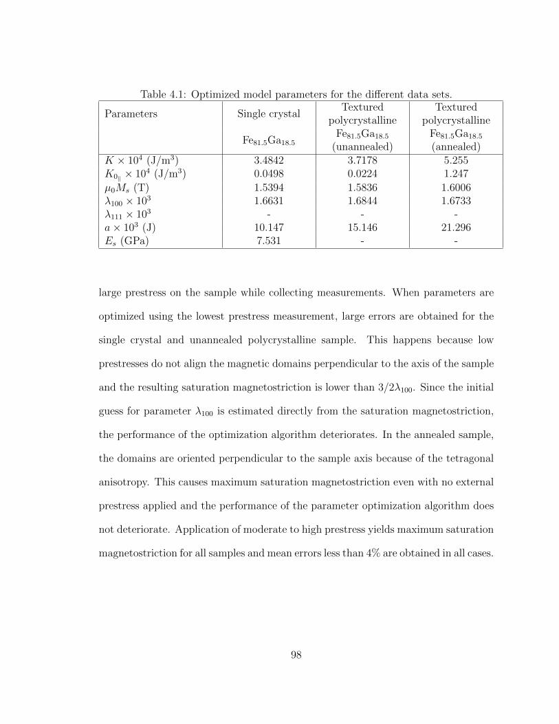
magnetomechanical response of both unannealed and annealed Galfenol. Table 4.1
lists down the optimized parameters obtained for all three cases. As expected, K0‖ is
substantially larger for the annealed sample as compared to the unannealed samples.
Also the smoothing factor for the textured polycrystalline samples is much larger
than the single crystal simple.
−50 0 50−2
−1.5
−1
−0.5
0
0.5
1
1.5
2
Field (kA/m)
Ind
uctio
n (
T)
−50 0 500
50
100
150
200
250
300
Field (kA/m)
Str
ain
(p
pm
)
De−hysterized data
Model
Figure 4.5: Anhysteretic model fit to the extracted anhysteretic curves with optimizedparameters for unannealed 〈100〉 textured polycrystalline Fe81.6Ga18.4. Measurementsare at constant compressive pre-stresses of 1.38 , 13.8, 27.6, 41.4, 55.2, 69.0, 82.7, and96.5 MPa.
From the point of view of the transducer designer, the utility of the parame-
ter optimization algorithm will be greatly enhanced if the model parameters can be
96
−50 0 50−2
−1.5
−1
−0.5
0
0.5
1
1.5
2
Field (kA/m)
Ind
uctio
n (
T)
−50 0 500
50
100
150
200
250
300
Field (kA/m)
Str
ain
(p
pm
)
De−hysterized data
Model
Figure 4.6: Anhysteretic model fit to the extracted anhysteretic curves with optimizedparameters for annealed 〈100〉 textured polycrystalline Fe81.6Ga18.4. Measurementsare at constant compressive pre-stresses of 1.38 , 13.8, 27.6, 41.4, 55.2, 69.0, 82.7, and96.5 MPa.
predicted accurately with reduced number of experiments. Usually actuation mea-
surements are simpler to perform than sensing measurements because it is easier to
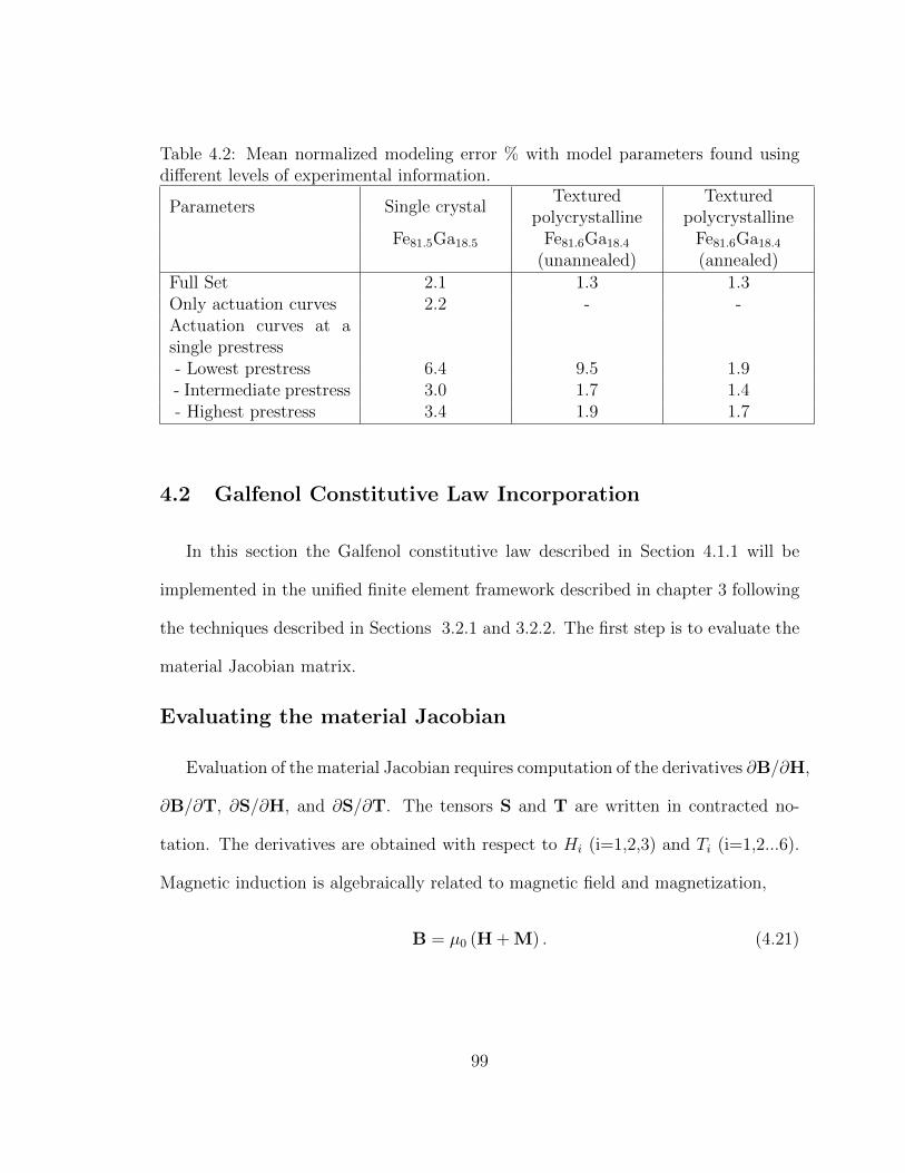
maintain a constant stress on the sample than constant field. Table 4.2 shows that
when the model parameters are optimized using only the actuation measurements for
the single crystal sample, the mean modeling error for all the curves (actuation and
sensing) increases by only 0.1%. Thus, sensing behavior can be accurately quantified
using actuation measurements.
The experimentation process can be further simplified if actuation measurements
at only one prestress could be used to estimate the model parameters. The prestress
applied on the sample could be anywhere between the lower and upper limit of the
working stress range. Table 4.2 shows that it is beneficial to have a moderate to
97
Table 4.1: Optimized model parameters for the different data sets.
Full Set 2.1 1.3 1.3Only actuation curves 2.2 - -Actuation curves at asingle prestress- Lowest prestress 6.4 9.5 1.9- Intermediate prestress 3.0 1.7 1.4- Highest prestress 3.4 1.9 1.7
4.2 Galfenol Constitutive Law Incorporation
In this section the Galfenol constitutive law described in Section 4.1.1 will be
implemented in the unified finite element framework described in chapter 3 following
the techniques described in Sections 3.2.1 and 3.2.2. The first step is to evaluate the
material Jacobian matrix.
Evaluating the material Jacobian
Evaluation of the material Jacobian requires computation of the derivatives ∂B/∂H,
∂B/∂T, ∂S/∂H, and ∂S/∂T. The tensors S and T are written in contracted no-
tation. The derivatives are obtained with respect to Hi (i=1,2,3) and Ti (i=1,2...6).
Magnetic induction is algebraically related to magnetic field and magnetization,
B = µ0 (H + M) . (4.21)
99
The derivatives of B with respect to Ti and Hi are
∂B
∂Ti= µ0
(∂M
∂Ti
), (4.22)
∂B
∂Hi
= µ0
(∂H
∂Hi
+∂M
∂Hi
). (4.23)
The derivatives of M and S with respect to Hi and Ti can be obtained by differenti-
ating (4.13) and (4.14),
∂M
∂Hi
=r∑
k=1
Ms
(∂mk
∂Hi
ξkan + mk ∂ξkan
∂Hi
), (4.24)
∂M
∂Ti=
r∑k=1
Ms
(∂mk
∂Tiξkan + mk ∂ξ
kan
∂Ti
), (4.25)
∂S
∂Hi
=r∑
k=1
(∂Sm
k
∂Hi
ξkan + Smk ∂ξ
kan
∂Hi
), (4.26)
∂S
∂Ti= s
∂T
∂Ti+
r∑k=1
(∂Sm
k
∂Tiξkan + Sm
k ∂ξkan
∂Ti
). (4.27)
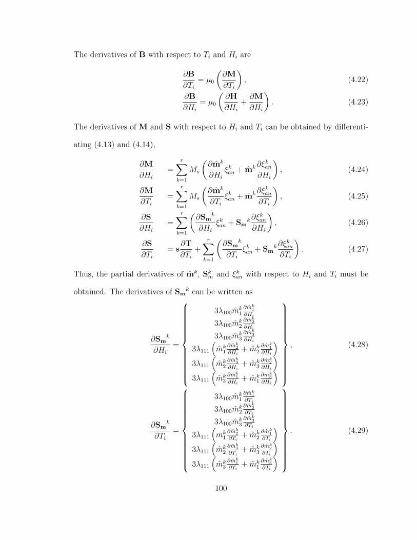
Thus, the partial derivatives of mk, Skm and ξkan with respect to Hi and Ti must be
obtained. The derivatives of Smk can be written as
∂Smk
∂Hi
=
3λ100mk1∂mk
1
∂Hi
3λ100mk2∂mk
2
∂Hi
3λ100mk3∂mk
3
∂Hi
3λ111
(mk
1∂mk
2
∂Hi+ mk
2∂mk
1
∂Hi
)3λ111
(mk
2∂mk
3
∂Hi+ mk
3∂mk
2
∂Hi
)3λ111
(mk
3∂mk
1
∂Hi+ mk
1∂mk
3
∂Hi
)
, (4.28)
∂Smk
∂Ti=
3λ100mk1∂mk
1
∂Ti
3λ100mk2∂mk
2
∂Ti
3λ100mk3∂mk
3
∂Ti
3λ111
(mk
1∂mk
2
∂Ti+ mk
2∂mk
1
∂Ti
)3λ111
(mk
2∂mk
3
∂Ti+ mk
3∂mk
2
∂Ti
)3λ111
(mk
3∂mk
1
∂Ti+ mk
1∂mk
3
∂Ti
)
. (4.29)
100
The derivatives of ξkan with respect to Hi and Ti can be found by differentiating (4.12),
∂ξkan∂Hi
=ξkanΩ
[r∑j=1
ξjan
(∂Gj
∂Hi
)−(∂Gk
∂Hi
)], (4.30)
∂ξkan∂Ti
=ξkanΩ
[r∑j=1
ξjan
(∂Gj
∂Ti
)−(∂Gk
∂Ti
)]. (4.31)
The derivatives of Gk with respect to Hi and Ti are
∂Gk
∂Hi
= mk ·K(∂mk
∂Hi
)− ∂mk
∂Hi
·Bk − mk ·(∂Bk
∂Hi
), (4.32)
∂Gk
∂Ti= mk ·K
(∂mk
∂Ti
)+
1
2mk ·
(∂K
∂Ti
)mk − ∂mk
∂Ti·Bk. (4.33)
The derivatives of the normalized kth equilibrium orientation with respect to Hi and
Ti are
∂mk
∂Hi
=1
‖mk‖∂mk
∂Hi
− mk
‖mk‖3
(mk · ∂mk
∂Hi
), (4.34)
∂mk
∂Ti=
1
‖mk‖∂mk
∂Ti− mk
‖mk‖3
(mk · ∂mk
∂Ti
), (4.35)
where
∂mk
∂Hi
= (K)−1
[∂Bk
∂Hi
−
(ck · (K)−1 ∂Bk
∂Hi
ck · (K)−1 ck
)ck
], (4.36)
∂mk
∂Ti= (K)−1
−(∂K
∂Ti
)mk +
ck ·(
(K)−1 ∂K∂Ti
mk)
ck · (K)−1 ckck
, (4.37)
∂Bk
∂H1
=
µ0Ms
00
,∂Bk
∂H2
=
0
µ0Ms
0
,∂Bk
∂H3
=
00
µ0Ms
, (4.38)
101
and
∂K
∂T1
=
−3λ100 0 00 0 00 0 0
, ∂K
∂T4
=
0 −3λ111 0−3λ111 0 0
0 0 0
,∂K
∂T2
=
0 0 00 −3λ100 00 0 0
, ∂K
∂T5
=
0 0 00 0 −3λ111
0 −3λ111 0
,∂K
∂T3
=
0 0 00 0 00 0 −3λ100
, ∂K
∂T6
=
0 0 −3λ111
0 0 0−3λ111 0 0
. (4.39)
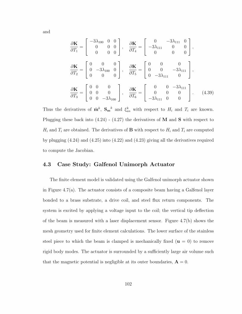
Thus the derivatives of mk, Smk and ξkan with respect to Hi and Ti are known.
Plugging these back into (4.24) - (4.27) the derivatives of M and S with respect to
Hi and Ti are obtained. The derivatives of B with respect to Hi and Ti are computed
by plugging (4.24) and (4.25) into (4.22) and (4.23) giving all the derivatives required
to compute the Jacobian.
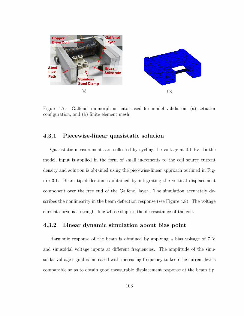
4.3 Case Study: Galfenol Unimorph Actuator
The finite element model is validated using the Galfenol unimorph actuator shown
in Figure 4.7(a). The actuator consists of a composite beam having a Galfenol layer
bonded to a brass substrate, a drive coil, and steel flux return components. The
system is excited by applying a voltage input to the coil; the vertical tip deflection
of the beam is measured with a laser displacement sensor. Figure 4.7(b) shows the
mesh geometry used for finite element calculations. The lower surface of the stainless
steel piece to which the beam is clamped is mechanically fixed (u = 0) to remove
rigid body modes. The actuator is surrounded by a sufficiently large air volume such
that the magnetic potential is negligible at its outer boundaries, A = 0.
102
(a) (b)
Figure 4.7: Galfenol unimorph actuator used for model validation, (a) actuatorconfiguration, and (b) finite element mesh.
4.3.1 Piecewise-linear quasistatic solution
Quasistatic measurements are collected by cycling the voltage at 0.1 Hz. In the
model, input is applied in the form of small increments to the coil source current
density and solution is obtained using the piecewise-linear approach outlined in Fig-
ure 3.1. Beam tip deflection is obtained by integrating the vertical displacement
component over the free end of the Galfenol layer. The simulation accurately de-
scribes the nonlinearity in the beam deflection response (see Figure 4.8). The voltage
current curve is a straight line whose slope is the dc resistance of the coil.
4.3.2 Linear dynamic simulation about bias point
Harmonic response of the beam is obtained by applying a bias voltage of 7 V
and sinusoidal voltage inputs at different frequencies. The amplitude of the sinu-
soidal voltage signal is increased with increasing frequency to keep the current levels
comparable so as to obtain good measurable displacement response at the beam tip.
103
0 5 10 150
50
100
150
Voltage (V)
Tip
deflection (
mic
rons)
Simulation
Experiment
(a)
0 5 10 150
0.5
1
1.5
2
2.5
Voltage (V)
Curr
ent (A
)
(b)
Figure 4.8: Quasistatic model results, (a) voltage-deflection, (b) voltage-current.
Figures 4.9-4.13 show the time-domain current and displacement response of the sys-
tem to sinusoidal voltage inputs ranging from 10 to 500 Hz. The model quantifies
the transient dynamic behavior of the beam for all the frequencies using a single set
of parameters. At the lower frequencies the model slightly over-predicts the response
because of its linear nature. As the frequency increases, the inertia and damping
forces dominate the force arising from the nonlinear internal stiffness, thus rendering
104
0 0.1 0.2 0.3 0.4−50
0
50
time (s)
Tip
de
fle
ctio
n (
mic
ron
s)
Experiment Simulation Error
(a)
0 0.1 0.2 0.3 0.4−0.4
−0.2
0
0.2
0.4
time(s)
Cu
rre
nt
(A)
(b)
Figure 4.9: Experimental and model results at 10 Hz, (a) tip displacement, (b) cur-rent.
0 0.02 0.04 0.06 0.08−40
−20
0
20
40
Tip
de
fle
ctio
n (
mic
ron
s)
time (s)
(a)
0 0.02 0.04 0.06 0.08−0.4
−0.2
0
0.2
0.4
time(s)
Cu
rre
nt
(A)
(b)
Figure 4.10: Experimental and model results at 50 Hz, (a) tip displacement, (b)current.
105
0 0.01 0.02 0.03 0.04 0.05 0.06
−20
−10
0
10
20
30
40
Tip
de
fle
ctio
n (
mic
ron
s)
time (s)
(a)
0 0.01 0.02 0.03 0.04 0.05 0.06−0.4
−0.2
0
0.2
0.4
time(s)
Cu
rre
nt
(A)
(b)
Figure 4.11: Experimental and model results at 100 Hz, (a) tip displacement, (b)current.
0 0.005 0.01 0.015 0.02 0.025 0.03
−10
0
10
20
30
Tip
de
fle
ctio
n (
mic
ron
s)
time (s)
(a)
0 0.005 0.01 0.015 0.02 0.025 0.03−0.2
−0.1
0
0.1
0.2
0.3
time(s)
Cu
rre
nt
(A)
(b)
Figure 4.12: Experimental and model results at 200 Hz, (a) tip displacement, (b)current.
106
0 0.005 0.01 0.015 0.02 0.025
−40
−20
0
20
40
Tip
de
fle
ctio
n (
mic
ron
s)
time (s)
(a)
0 0.005 0.01 0.015 0.02 0.025
−0.15
−0.1
−0.05
0
0.05
0.1
time(s)
Cu
rre
nt
(A)
(b)
Figure 4.13: Experimental and model results at 500 Hz, (a) tip displacement, (b)current.
the response more smooth. This leads to better correlation between the amplitudes
of the modeled and experimental curves. However, because the model does not con-
sider hysteresis in Galfenol, there is a phase difference between the experimental and
modeled curves which is negligible till 100 Hz but becomes more noticeable at the
higher frequencies. At 200 Hz the measured displacement response is distorted, pos-
sibly because some nonlinearities in the material are excited at that frequency due
to a particular distribution of stress and field. Since the dynamic model is linear in
nature, this effect is not described. The measured current response is undistorted
and is accurately described. At 500 Hz the transient tip deflection response exhibits
beating behavior, as the excitation frequency is close to the first natural frequency of
the actuator (513 Hz). When the harmonic excitation is switched on, the fundamental
mode is also excited which interacts with components at the drive frequency giving
rise to beats. The current takes a few cycles to reach steady state and the response
looks typical of a damped second order system.
107
4.3.3 Nonlinear dynamic simulation
The same Galfenol unimorph actuator (Figure 4.7) is used to validate the nonlinear
dynamic solution procedure. Harmonic excitations ranging from 10 Hz to 200 Hz are
applied to the system in the form V (t) = −Vbias + V0(1 − cos(ωdrt)), where ωdr is
the excitation frequency. The finite element model is run only for the time duration
of the first few cycles. In order to obtain appreciable displacement response from
the beam at higher frequencies, a negative bias voltage (Vbias) is applied first before
applying the harmonic signal. This ensures that the effective bias point of the cyclic
signal is in the burst region. In the model the bias point is obtained in similar fashion
by applying the bias voltage smoothed using a hyperbolic tangent function for ease
of convergence. Figures 4.14 - 4.17 show the transient response of the transducer
for harmonic inputs at 10, 50, 100, and 200 Hz. The modeled responses show good
correlation with the experiments particularly for the tip deflection response. An
interesting outcome of nonlinear Galfenol behavior can be seen where the quadratic
nonlinearity of the magnetostrictive strain at zero field causes frequency doubling in
the tip deflection response.
4.4 Concluding Remarks
Nonlinear Galfenol constitutive behavior was successfully incorporated in the
unified finite element modeling framework described earlier and validated using a
Galfenol unimorph actuator. The piecewise-linear procedure is useful for obtaining
quasistatic system response and accurate bias point determination. A linear dynamic
simulation with the Galfenol material coefficients computed at the bias point pro-
vides an accurate description of system dynamics for moderate inputs. An implicit
108
0 0.05 0.1 0.15 0.2
0
20
40
60
80
100
Tip
dis
pla
cem
ent (m
icro
ns)
Time (s)0 0.05 0.1 0.15 0.2
−0.5
0
0.5
1
1.5
Curr
ent (A
)
Time (s)
Model
Data
Error
Figure 4.14: Actuator response to harmonic excitation at 10 Hz.
0 0.02 0.04 0.06
0
20
40
60
80
Tip
dis
pla
cem
ent (m
icro
ns)
Time (s)0 0.02 0.04 0.06
−0.5
0
0.5
1
Time (s)
Curr
ent (A
)
Model
Data
Error
Figure 4.15: Actuator response to harmonic excitation at 50 Hz.
0.01 0.02 0.03 0.04
0
20
40
60
Tip
dis
pla
cem
ent (m
icro
ns)
Time (s)
0.01 0.02 0.03 0.04−1
−0.5
0
0.5
1
Curr
ent (A
)
Time (s)
Model
Data
Error
Figure 4.16: Actuator response to harmonic excitation at 100 Hz.
109
0 0.005 0.01 0.015 0.02−20
0
20
40
60
80
100
Tip
dis
pla
cem
ent (m
icro
ns)
Time (s)0 0.005 0.01 0.015 0.02
−1.5
−1
−0.5
0
0.5
1
Time (s)
Curr
ent (A
)
Model
Data
Error
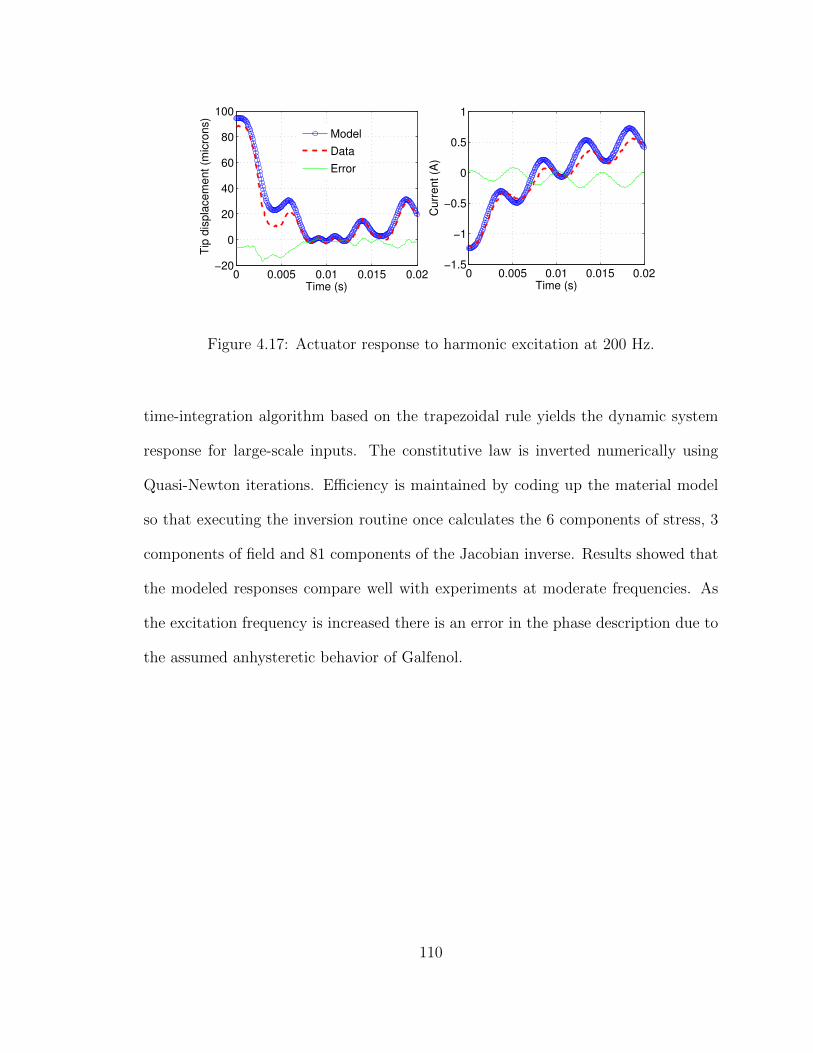
Figure 4.17: Actuator response to harmonic excitation at 200 Hz.
time-integration algorithm based on the trapezoidal rule yields the dynamic system
response for large-scale inputs. The constitutive law is inverted numerically using
Quasi-Newton iterations. Efficiency is maintained by coding up the material model
so that executing the inversion routine once calculates the 6 components of stress, 3
components of field and 81 components of the Jacobian inverse. Results showed that
the modeled responses compare well with experiments at moderate frequencies. As
the excitation frequency is increased there is an error in the phase description due to
the assumed anhysteretic behavior of Galfenol.
110
Chapter 5: TERFENOL-D TRANSDUCERS
Magnetostrictive Terfenol-D (Tb0.7Dy0.3Fe2) is attractive for practical actuators
due to its large magnetostriction (1600 ppm) and moderate saturation fields (200 kA/m).
This chapter aims at applying the unified framework developed in Chapter 3 to
model Terfenol-D transducers. First, a fully coupled 3D energy averaged model is
derived, which describes the magnetomechanical behavior of Terfenol-D. Due to the
poor machinability of Terfenol-D, they are mostly available in 1D geometries like
cylindrical rods. Thus most Terfenol-D transducers are axisymmetric in nature with
the permanent magnet and flux return components concentric with the Terfenol-D
driver. To take advantage of this, the 3D finite element model is reduced to a 2D
axisymmetric form. It is then used to conduct a parametric study on a hydraulically
amplified Terfenol-D actuator designed for use in active engine mounts.
5.1 Fully Coupled Discrete Energy Averaged Model for Terfenol-D
Modeling the constitutive behavior of Terfenol-D has traditionally been a difficult
problem. The presence of a large magnetostriction anisotropy, low magnetocrystalline
anisotropy, and a twinned dendritic structure gives rise to complex domain level pro-
cesses which are not completely understood [42]. The aim of this work is to describe
111
the actuation and sensing response of Terfenol-D over a wide range of magnetic field
and stress values using an efficient energy-averaged constitutive model which can be
used for design and control of Terfenol-D transducers.
The Jiles-Atherton model [49] was originally formulated for isotropic ferromagnetic
hysteresis. The total magnetization of a ferromagnetic material with Weiss-type mo-
ment interactions is obtained as the sum of an irreversible component due to domain
wall motion and a reversible component due to domain wall bowing. With careful
understanding of the difference between local and global anhysteretic responses [29],
the model is straightforward to implement and computationally efficient, as it involves
only five parameters which can be directly correlated to measurements. For this rea-
son, the Jiles-Atherton model has been used to describe the behavior of Terfenol-D
actuators in which the magnetostriction is modeled as a quadratic function of mag-
netization [11, 41, 14].
The Preisach model [66] generates smooth ferromagnetic hysteresis curves through
contributions from a large number of elementary bistable hysterons. Because giant
magnetostrictive materials such as Terfenol-D show significant deviation in behavior
from elementary Preisach hysterons, Reimers and Della Torre [70, 71] developed a
special hysteron with a bimodally distributed susceptibility function to model the 1D
actuation response of Terfenol-D.
Carman et al. [12] formulated a model for Terfenol-D using Gibbs free energy
expanded in a Taylor series. The exact form of the series, that is the degree of trun-
cation, and the value of the coefficients were dictated by experimental measurements.
The model describes Terfenol-D actuation for low to moderate applied fields over a
specific range of applied pre-stress. Zheng et al. [91] included higher order terms in
112
the Taylor series expansion of Gibbs energy and used a Langevin function to describe
the magnetization curve. The model, although anhysteretic, accurately describes the
nonlinear nature of Terfenol-D’s magnetostriction for a wide range of pre-stresses.
The ∆E effect is also modeled but validated only qualitatively.
Armstrong et al. [3] formulated a model for Terfenol-D in which bulk magnetiza-
tion and strain are obtained as an expected value of a large number of possible energy
states (or moment orientations) with an energy based probability density function.
To increase the model efficiency, Armstrong et al. [2] restricted the choice of moment
orientations to the easy magnetization axes (eight 〈111〉 directions for Terfenol-D) and
used a discrete version of the probability density function. The increase in compu-
tational speed, however, came at the cost of reduced accuracy. To preserve accuracy
without sacrificing efficiency, Evans and Dapino [32] developed a constitutive model
for Galfenol by choosing orientations which minimize an energy functional locally de-
fined about each easy axis direction. This energy averaged model has major shortcom-
ings when applied to Terfenol-D as detailed in Section 5.1.1. Section 5.1.2 presents an
anhysteretic model formulation that addresses each of those challenges; anhysteretic
model results are compared with experimental measurements in Section 5.1.3. The
proposed anhysteretic version of the model is fully 3D and appropriate for use in
finite element modeling frameworks. An extension to model magnetomechanical hys-
teresis is done in section 5.1.4 by using an evolution equation for the domain volume
fractions similar to Evans et al. [32] The hysteretic model can be used for control ap-
plications where quantification of additional delay due to material hysteresis is critical
for ensuring stability. Section 5.1.5 provides a quantitative description of the model
performance.
113
5.1.1 Problem description
Terfenol-D has eight minima along the 〈111〉 directions. When energy averaged
models such as the Armstrong model [2] or the Discrete Energy Averaged Model
(DEAM) [32] are compared with measurements, two major discrepancies are ob-
served. First, these models introduce an extra kink in the magnetization and mag-
netostriction and secondly, the experimentally observed slow approach to saturation
is absent (Figure 5.1). Using a sufficiently high smoothing factor (as done by Arm-
strong [2]) removes the unphysical kink and somewhat smooths out the saturation
behavior. However, it results in large inaccuracies in the low to moderate field re-
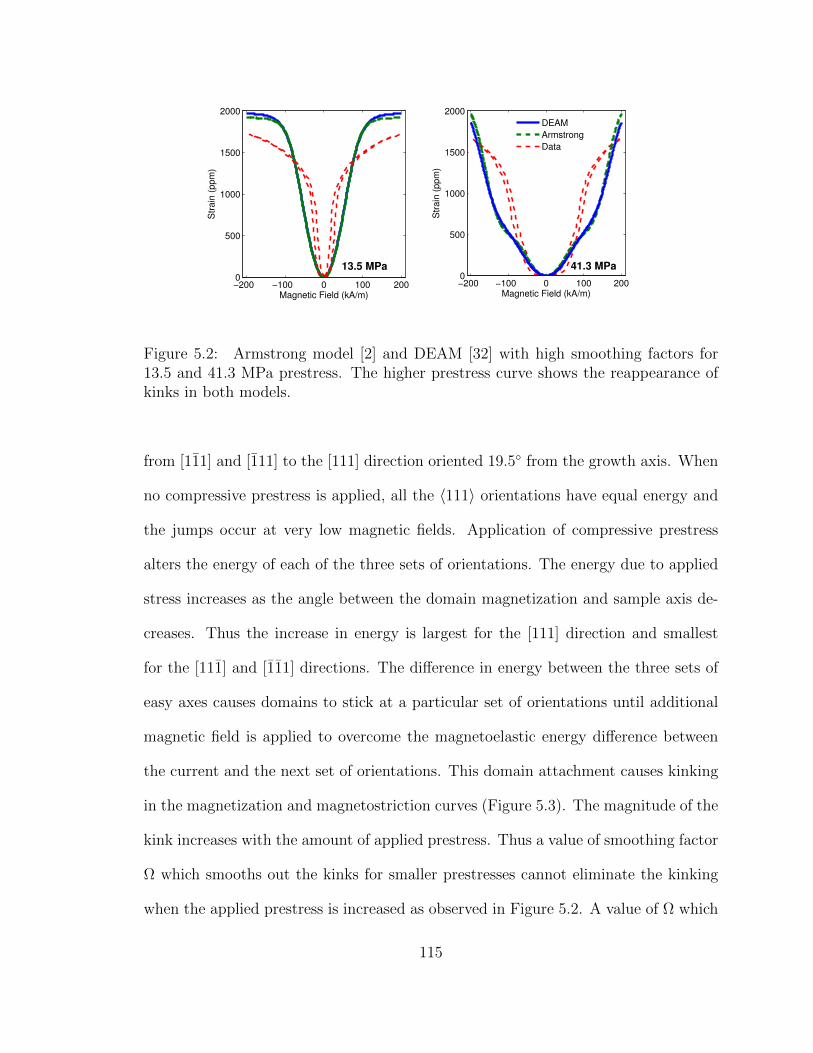
gions. Moreover, the kinking reappears at high pre-stress values (Figure 5.2). For a
−200 −100 0 100 200−1.5
−1
−0.5
0
0.5
1
1.5
Field (kA/m)
µ0 M
(T
)
−200 −100 0 100 2000
500
1000
1500
2000
2500
Field (kA/m)
Str
ain
(p
pm
)
DEAM
Armstrong
Data
Figure 5.1: Comparison of magnetization and magnetostriction curves for Terfenol-Dat 13.5 MPa compressive stress [31] with the Armstrong model [2] and the DiscreteEnergy Averaged Model (DEAM) [32].
[112]-oriented sample, the magnetization process is governed by two distinct domain
jumps: one from the [111] and [111] directions perpendicular to the sample axis to the
[111] and [111] directions oriented 61.9 from the sample growth axis, and the second
114
−200 −100 0 100 2000
500
1000
1500
2000
Magnetic Field (kA/m)
Str
ain
(ppm
)
−200 −100 0 100 2000
500
1000
1500
2000
Magnetic Field (kA/m)
Str
ain
(ppm
)
DEAM
Armstrong
Data
13.5 MPa 41.3 MPa
Figure 5.2: Armstrong model [2] and DEAM [32] with high smoothing factors for13.5 and 41.3 MPa prestress. The higher prestress curve shows the reappearance ofkinks in both models.
from [111] and [111] to the [111] direction oriented 19.5 from the growth axis. When
no compressive prestress is applied, all the 〈111〉 orientations have equal energy and
the jumps occur at very low magnetic fields. Application of compressive prestress
alters the energy of each of the three sets of orientations. The energy due to applied
stress increases as the angle between the domain magnetization and sample axis de-
creases. Thus the increase in energy is largest for the [111] direction and smallest
for the [111] and [111] directions. The difference in energy between the three sets of
easy axes causes domains to stick at a particular set of orientations until additional
magnetic field is applied to overcome the magnetoelastic energy difference between
the current and the next set of orientations. This domain attachment causes kinking
in the magnetization and magnetostriction curves (Figure 5.3). The magnitude of the
kink increases with the amount of applied prestress. Thus a value of smoothing factor
Ω which smooths out the kinks for smaller prestresses cannot eliminate the kinking
when the applied prestress is increased as observed in Figure 5.2. A value of Ω which
115
−200 −100 0 100 2000
500
1000
1500
2000
2500
Field (kA/m)
Str
ain
(ppm
)
−200 −100 0 100 2000
500
1000
1500
2000
2500
Field (kA/m)
Str
ain
(ppm
)
Increasing pre−stress [111], [111]
DEAMArmstrong
[111], [111]
Increasing pre−stress
[111], [111]
Figure 5.3: Armstrong model [2] and DEAM [32] with low smoothing factors showingthe magnitude of the two kinks with increasing stress.
is high enough to smooth out the kinks for all prestresses results in the model overes-
timating the burst field and underestimating the slope of the magnetostriction-field
curve in the burst region. These issues imply that fundamental changes need to be
made in order to apply energy-averaged models to Terfenol-D.
5.1.2 Model formulation
Elimination of extra kinks
Assuming a [112]-oriented sample, the intermediate kinks occur when domains
align along the [111] and [111] directions for positive applied fields and [111] and
[111] directions for negative applied fields. Absence of kinks in the measurements
suggests that domains are prevented from orienting along these directions. This
can be modeled by increasing the magnetocrystalline anisotropy energy along these
orientations compared to the other easy axis orientations. In the original DEAM
116
formulation, the anisotropy energy is defined locally around each easy axis as
GkA =
1
2Kk‖mk − ck‖2, (5.1)
where the anisotropy constant Kk controls how steep the anisotropy energy wells are
around the kth easy axis ck. Since the anisotropy energy along each easy axis direction
is identically zero, achieving variations in the base anisotropy energy between the
different easy axes is not possible. To achieve such variation an orientation-dependent
global anisotropy energy is superimposed onto the local anisotropy energy defined
around each easy axis direction as
GkA = wkGk
A0+
1
2Kk‖mk − ck‖2. (5.2)
Here, GkA0
is the global anisotropy energy, which for materials with cubic anisotropy
is given by
GkA0
= K4(mk2
1 mk2
2 +mk2
2 mk2
3 +mk2
3 mk2
1 ) +K6(mk2
1 mk2
2 mk2
3 ), (5.3)
In (5.2), GkA0
is weighted by wk, an empirical weighting factor which adjusts the
anisotropy energy along the kth easy axis. Physically, the weighting accounts for the
change in energy landscape that may occur due to precipitates, dislocations and twin
boundaries [1]. The 8 easy axes can be broken down into 3 groups depending upon
their angle with the sample axis: the [111] and [111] directions oriented 19.5 with
the sample axis, the [111] and [111] directions oriented perpendicular to the sample
axis, and the [111], [111], [111], and [111] directions oriented 61.9 from the sample
axis. Thus, there are effectively three weights which must be determined, one for
each group.
Another way to suppress the kinks is to ignore the minima associated with the
four orientations which cause kinking. The global anisotropy energy is still weighted
117
but there are only two weights to be determined since the set of directions 61.9 from
the sample axis is not considered. This way the number of minima is reduced to
four. The first approach is more accurate as it has more degrees of freedom while the
second approach is more efficient as it involves averaging of only four terms. However,
in the second approach, the three dimensional accuracy of the model is expected to
suffer due to the loss of four orientations. In this paper the full version of the model
is described in detail and its performance is compared to the reduced version in terms
of accuracy and efficiency.
Obtaining the slow approach to saturation
The exact reason for the slow approach to saturation in Terfenol-D is not clearly
understood. Various explanations have been proposed such as the presence of demag-
netization fields [89], or radically different behavior of twins [25], but experimental
proof is lacking. Domain observations reported by Engdahl [31] suggest that clo-
sure domains become increasingly difficult to remove in Terfenol-D as the sample is
magnetized. From these theories and observations it can be postulated that with
increasing applied field, there is a tendency of domains to occupy orientations which
do not minimize the theoretical energy obtained by summing up the anisotropic,
magnetoelastic and Zeeman components. Incorporation of demagnetization fields in
the model comes at the expense of an implicit definition for the total energy which
means that iterations need to be performed to converge to the correct value of volume
fractions. Every iteration will involve computation of the energies, minima, domain
volume fractions, and the bulk magnetization ,adding significant computational effort
to the model.
118
An alternative way of incorporating this apparent broadening of domain distribu-
tion is to employ a variable smoothing factor which increases as the domain volume
fractions move farther and farther away from a homogeneous distribution. Mathe-
matically this can be written as
Ω = a0 + a1‖ξan(H,T)− ξ‖2, (5.4)
where ξan(H,T) is the vector of anhysteretic domain volume fractions and ξ is a
vector equal in length to ξan but with each component as 1/r, r being the number
of easy axis orientations. Both ξan and ξ are r-dimensional vectors, with r = 8 for
Terfenol-D. When no bias stress or field is applied, assuming cubic magnetocrystalline
anisotropy energy distribution, all 8 orientations are equally likely to be occupied by
the domains. Thus ξan = ξ and Ω = a0, its lowest value. On application of stress
or field the volume fractions will deviate away from this homogeneous distribution
causing Ω to increase. When a bias stress or field is applied, the initial domain
distribution is not homogeneous, so for application of field and stress about the bias
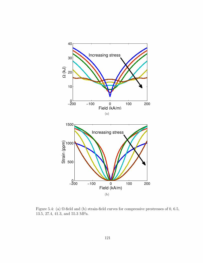
points Ω does no longer increase monotonically. Figure 5.4(a) shows the variation
of Ω with applied field for different bias stress values. At low fields the value of Ω
increases with increasing bias stress while at high fields Ω is larger for a lower bias
stress. This allows the magnetostriction curves for low bias stress to exhibit a sharp
burst region at low fields and a gradual approach to saturation at high fields, while
for the high bias stress curves the slope in the burst region is more gradual since Ω
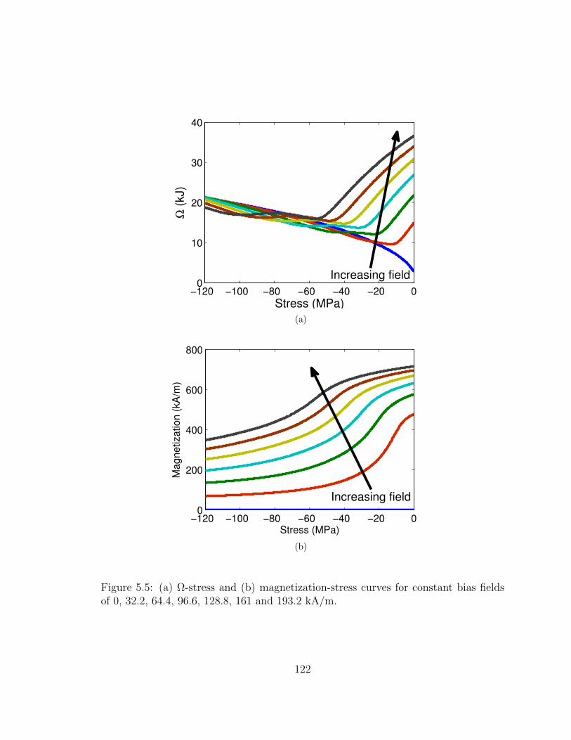
is relatively large in the burst region (Figure 5.4(b)). Figure 5.5 shows the Ω–stress
curves and the corresponding magnetization-stress curves for different bias fields. For
low bias fields, Ω is small at low stresses and larger at higher stress values while for
high bias fields, Ω is large for low stresses and relatively small for higher stress values.
119
Due to the large values of Ω at high bias fields and low stresses, the M-H curves
display very gradual saturation in the low stress region. Thus, even for very high bias
fields, application of stress almost immediately results in magnetization decrease due
to the broad domain distribution. These variations are shown for a crystal having
perfect cubic anisotropy. When the anisotropy is weighted as described previously,
these variations in Ω will change since at zero applied stress and field the domains
will not be homogeneously distributed among the eight directions. Rather they will
be concentrated in orientations along which the global anisotropy energy weight is
the maximum.
Computational aspects
The computation proceeds in a manner identical to the Galfenol constitutive law
up to the computation of the minima. Since the m-dependent portion of the energy
is identical in both cases, expression (4.10) still yield the energy minima. For imple-
mentation in finite element models, the computed minima are normalized to prevent
unphysical behavior at high fields similar to the Galfenol constitutive model.
The new definition for Ω, expression (5.4), destroys the explicit nature of the
model since Ω is defined as a function of ξan while determination of ξan requires
knowledge of Ω according to the relation
ξkan =exp
(−Gk/Ω(ξan)
)∑rj=1 exp (−Gj/Ω(ξan))
, (5.5)
where ξkan is the volume fraction of the kth easy axis. The difference between this
implicit definition and having an implicit definition for energy (as in the case of
demagnetization fields) is that here the energy expressions and therefore the minima
remain unchanged in every iteration. Only the volume fractions need to be computed
120
−200 −100 0 100 2000
10
20
30
40
Ω (
kJ)
Field (kA/m)
Increasing stress
(a)
−200 −100 0 100 2000
500
1000
1500
Field (kA/m)
Str
ain
(ppm
)
Increasing stress
(b)
Figure 5.4: (a) Ω-field and (b) strain-field curves for compressive prestresses of 0, 6.5,13.5, 27.4, 41.3, and 55.3 MPa.
121
−120 −100 −80 −60 −40 −20 00
10
20
30
40
Stress (MPa)
Ω (
kJ)
Increasing field
(a)
−120 −100 −80 −60 −40 −20 00
200
400
600
800
Stress (MPa)
Magnetization (
kA
/m)
Increasing field
(b)
Figure 5.5: (a) Ω-stress and (b) magnetization-stress curves for constant bias fieldsof 0, 32.2, 64.4, 96.6, 128.8, 161 and 193.2 kA/m.
122
again. This is illustrated by the flowchart shown in Figure 5.13. The solution loop
involves combining (5.4) and (5.5) to obtain a single equation in terms of Ω, giving
f(Ω) = Ω− a0 − a1
r∑k=1
(ξkan − ξk
)2= 0. (5.6)
Newton-Raphson iterations are performed for quick convergence since the derivative
df/dΩ can be analytically obtained as
df
dΩ= 1− 1
Ω2
r∑k=1
2a1
(ξkan − ξ
k)(
ξkanGk − ξkan
r∑j=1
ξjanGj
). (5.7)
Even with strict tolerances, usually two to three iterations are sufficient for conver-
gence. To investigate the effect of this iterative procedure on the model efficiency,
the model is run with and without iterations for a large number of inputs. It is found
that on an average the iterative version takes only 20 % longer than the non-iterative
one.
5.1.3 Anhysteretic model results
The model is compared with actuation measurements from Moffett et al. [62] and
sensing measurements from Kellogg et al. [51] Anhysteretic model parameters have
been obtained by extracting the anhysteretic curves from data (using simple averaging
of values from the upper and lower branches of the major hysteresis loops [8]) and
using a least squares optimization algorithm. The full model with 8 minima contains
the model with 4 minima contains 8 parameters due to the absence of w5 through w8.
Figure 5.7 shows the performance of the two models when optimized to describe
the magnetostriction measurements of Moffett et al. Both models can describe the
measurements. However, the reduced version shows some error near saturation partic-
ularly for the high bias stress curves. With parameters optimized for the strain-field
123
Figure 5.6: Flowchart for the anhysteretic model. Details of the energy minimizationis shown in section 4.1.1.
124
0 50 100 150 200 250 300 350 4000
200
400
600
800
1000
1200
1400
1600
1800
Str
ain
(ppm
)
Field (kA/m)
Data
Model (8 minima)
Model (4 minima)
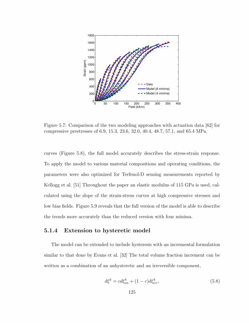
Figure 5.7: Comparison of the two modeling approaches with actuation data [62] forcompressive prestresses of 6.9, 15.3, 23.6, 32.0, 40.4, 48.7, 57.1, and 65.4 MPa.
curves (Figure 5.8), the full model accurately describes the stress-strain response.
To apply the model to various material compositions and operating conditions, the
parameters were also optimized for Terfenol-D sensing measurements reported by
Kellogg et al. [51] Throughout the paper an elastic modulus of 115 GPa is used, cal-
culated using the slope of the strain-stress curves at high compressive stresses and
low bias fields. Figure 5.9 reveals that the full version of the model is able to describe
the trends more accurately than the reduced version with four minima.
5.1.4 Extension to hysteretic model
The model can be extended to include hysteresis with an incremental formulation
similar to that done by Evans et al. [32] The total volume fraction increment can be
written as a combination of an anhysteretic and an irreversible component,
dξk = cdξkan + (1− c)dξkirr, (5.8)
125
−80 −70 −60 −50 −40 −30 −20 −10 0
0
500
1000
1500
2000
Stress (MPa)
Str
ain
(ppm
)
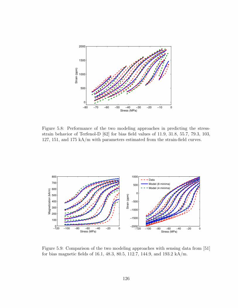
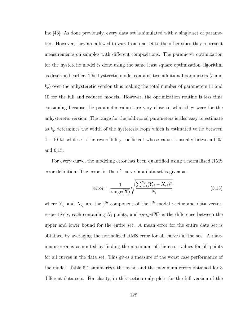
Figure 5.8: Performance of the two modeling approaches in predicting the stress-strain behavior of Terfenol-D [62] for bias field values of 11.9, 31.8, 55.7, 79.3, 103,127, 151, and 175 kA/m with parameters estimated from the strain-field curves.
−120 −100 −80 −60 −40 −20 00
100
200
300
400
500
600
700
800
Stress (MPa)
Ma
gn
etiza
tio
n (
kA
/m)
−120 −100 −80 −60 −40 −20 0−2000
−1500
−1000
−500
0
500
1000
Stress (MPa)
Str
ain
(p
pm
)
Data
Model (8 minima)
Model (4 minima)
Figure 5.9: Comparison of the two modeling approaches with sensing data from [51]for bias magnetic fields of 16.1, 48.3, 80.5, 112.7, 144.9, and 193.2 kA/m.
The calculation of partial derivatives ∂ξkan/∂H and ∂ξkan/∂T for the traditional energy-
averaged model is simple since ξkan is explicitly defined in terms of H and T. In this
case ξkan is implicit as given by (5.5). But, it is still possible to obtain an analytical
expression for its derivatives given by
∂ξkan∂Hi
= αk − ξkanr∑j=1
αj + 2a1
(ξan − ξ
)·(dξandHi
)(βk − ξkan
r∑j=1
βj
), (5.11)
where
αk = −ξkan
a
(∂Gk
∂Hi
), (5.12)
βk =ξkana2Gk, (5.13)
(ξan − ξ
)·(dξandHi
)=
∑rk=1
(αk − ξkan
∑rj=1 α
j)(
ξkan − ξk)
1− 2a1
∑rk=1
(βk − ξkan
∑rj=1 β
j)(
ξkan − ξk) . (5.14)
The derivatives ∂Gk/∂Hi can be obtained similar to (4.32). Equation (5.14) is ob-
tained by multiplying (5.11) by(ξkan − ξk
)and summing for all k. The partial deriva-
tives with respect to Ti can be computed following a similar procedure.
5.1.5 Hysteretic model results
The performance of the hysteretic model is described quantitatively in this section
by comparing it with the same data sets. Additionally, the parameters have been op-
timized to describe Terfenol-D magnetostriction data supplied by Etrema Products,
127
Inc [43]. As done previously, every data set is simulated with a single set of parame-
ters. However, they are allowed to vary from one set to the other since they represent
measurements on samples with different compositions. The parameter optimization
for the hysteretic model is done using the same least square optimization algorithm
as described earlier. The hysteretic model contains two additional parameters (c and
kp) over the anhysteretic version thus making the total number of parameters 11 and
10 for the full and reduced models. However, the optimization routine is less time
consuming because the parameter values are very close to what they were for the
anhysteretic version. The range for the additional parameters is also easy to estimate
as kp determines the width of the hysteresis loops which is estimated to lie between
4 – 10 kJ while c is the reversibility coefficient whose value is usually between 0.05
and 0.15.
For every curve, the modeling error has been quantified using a normalized RMS
error definition. The error for the ith curve in a data set is given as
error =1
range(X)
√∑Ni
j=1(Yij −Xij)2
Ni
. (5.15)
where Yij and Xij are the jth component of the ith model vector and data vector,
respectively, each containing Ni points, and range(X) is the difference between the
upper and lower bound for the entire set. A mean error for the entire data set is
obtained by averaging the normalized RMS error for all curves in the set. A max-
imum error is computed by finding the maximum of the error values for all points
for all curves in the data set. This gives a measure of the worst case performance of
the model. Table 5.1 summarizes the mean and the maximum errors obtained for 3
different data sets. For clarity, in this section only plots for the full version of the
128
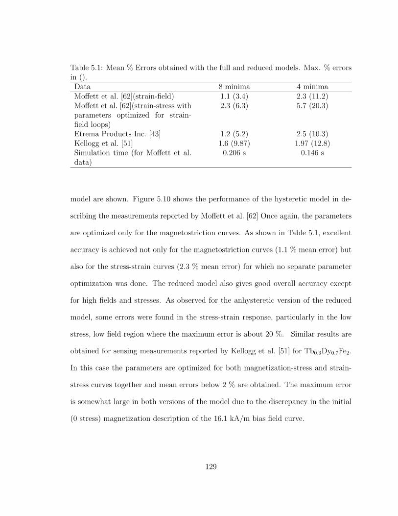
Table 5.1: Mean % Errors obtained with the full and reduced models. Max. % errorsin ().Data 8 minima 4 minimaMoffett et al. [62](strain-field) 1.1 (3.4) 2.3 (11.2)Moffett et al. [62](strain-stress withparameters optimized for strain-field loops)
2.3 (6.3) 5.7 (20.3)
Etrema Products Inc. [43] 1.2 (5.2) 2.5 (10.3)Kellogg et al. [51] 1.6 (9.87) 1.97 (12.8)Simulation time (for Moffett et al.data)
0.206 s 0.146 s
model are shown. Figure 5.10 shows the performance of the hysteretic model in de-
scribing the measurements reported by Moffett et al. [62] Once again, the parameters
are optimized only for the magnetostriction curves. As shown in Table 5.1, excellent
accuracy is achieved not only for the magnetostriction curves (1.1 % mean error) but
also for the stress-strain curves (2.3 % mean error) for which no separate parameter
optimization was done. The reduced model also gives good overall accuracy except
for high fields and stresses. As observed for the anhysteretic version of the reduced
model, some errors were found in the stress-strain response, particularly in the low
stress, low field region where the maximum error is about 20 %. Similar results are
obtained for sensing measurements reported by Kellogg et al. [51] for Tb0.3Dy0.7Fe2.
In this case the parameters are optimized for both magnetization-stress and strain-
stress curves together and mean errors below 2 % are obtained. The maximum error
is somewhat large in both versions of the model due to the discrepancy in the initial
(0 stress) magnetization description of the 16.1 kA/m bias field curve.
129
0 100 200 300 4000
200
400
600
800
1000
1200
1400
1600
1800
Field (kA/m)
Str
ain
(p
pm
)
Data
Model
−80 −60 −40 −20 00
500
1000
1500
2000
Stress (MPa)
Str
ain
(p
pm
)
Figure 5.10: Comparison of hysteretic model with data from Moffett et al [62] forcompressive prestresses of 6.9, 15.3, 23.6, 32.0, 40.4, 48.7, 57.1, and 65.4 MPa. Pa-rameters optimized for actuation curves.
−100 −50 00
100
200
300
400
500
600
700
800
Stress (MPa)
Magnetization (
kA
/m)
−100 −50 0−2000
−1500
−1000
−500
0
500
1000
Stress (MPa)
Str
ain
(ppm
)
Data
Model
Figure 5.11: Comparison of hysteretic model with sensing data from Kellogg et al [62]for bias magnetic fields of 16.1, 48.3, 80.5, 112.7, 144.9, and 193.2 kA/m.
130
Finally, the parameters are optimized to describe the magnetostriction curves
for commercially available Terfenol-D supplied by Etrema Products, Inc. [43] (Fig-
ure 5.12). Not only does the model describe the nonlinear nature of the response with
accuracy but it also quantifies the hysteretic regions very accurately. For example,
at high compressive prestresses, the magnetization process is dominated by reversible
domain rotation giving rise to a nearly anhysteretic response. This is seen both in the
experimental and modeled magnetostriction curves at 16 ksi (110.4 MPa). The model
also describes the effect of preload on the maximum magnetostriction. For example,
the 1 ksi (6.9 MPa) curve exhibits a lower saturation magnetostriction than the 4 ksi
(27.6 MPa) and 8 ksi (55.2 MPa) curves. The optimized parameters for every data
set for both versions of the model are shown in Table 5.2. To compare the efficiencies
of the two models, the time taken by each to simulate the Moffett et al. [62] data set
is clocked in Matlab. The reduced model takes about 30 % less time than the full
version. Thus, the reduced version can be used in applications where some accuracy
can be sacrificed in the interest of computational speed.
5.1.6 Concluding remarks
The energy averaged model derived in this chapter addressed two main discrepan-
cies of previous energy averaged models in modeling Terfenol-D response - presence
of an unphysical kink in the modeled response which is absent in measurements and
absence of the slow approach to saturation present in Terfenol-D magnetostriction.
Use of a weighted global anisotropy energy combined with a variable smoothing factor
based on the deviation of domain volume fractions from a homogeneous distribution
is able to tackle both issues successfully. The anhysteretic model is fully 3D in nature
131
Tab
le5.
2:O
pti
miz
edm
odel
par
amet
ers
for
the
diff
eren
tdat
ase
ts.
Moff
ett
etal
.[6
2]K
ello
gget
al.
[51]
Etr
ema
Pro
duct
sIn
c.[4
3]
Par
amet
ers
8m
inim
a4
min
ima
8m
inim
a4
min
ima
8m
inim
a4
min
ima
K×
105
(J/m
3)
4.30
62.
409
17.6
83.
049
4.60
22.
188
µ0M
s(T
)1.
025
0.89
21.
047
0.97
50.
964
0.89
1
λ100×
103
0.11
40.
126
0.09
30.
114
0.10
40.
094
λ111×
103
1.54
61.
554
1.48
61.
348
1.42
41.
428
a0×
103
(J)
1.77
60.
600
4.61
17.
202
1.93
0.6
a1×
103
(J)
92.4
915
0.4
44.6
950
.743
.11
70.7
7
w(1,2
)1.
119
1.14
91.
341
1.25
21.
068
1.06
2
w(3,4
)0.
940
0.84
60.
844
0.74
81.
056
1.06
1
w(5,6,7,8
)0.
915
–0.
575
–0.
873
–
kp×
103
(J)
5.58
24.
215
8.37
67.
802
109.
297
c0.
150.
150.
100
0.10
40.
050.
05
Es
(GP
a)11
511
511
511
511
511
5
132
−300 −200 −100 0 100 200 3000
500
1000
1500
2000
Str
ain
(p
pm
)
Field (kA/m)
Data
Model
Figure 5.12: Comparison of hysteretic model with magnetostriction measurementsprovided by Etrema Products Inc. [43] for compressive prestresses of 1, 4, 8, and16 KSI (6.9, 27.6, 55.2, 110.4 MPa).
and is appropriate for incorporating into the finite element framework of Chapter 3.
Although the addition of an implicit relationship for the domain volume fractions
requires the need for equilibrium iterations to achieve convergence, the model takes
only 20% longer time than its non-iterative counterpart. A hysteretic extension to the
model is formulated based on an evolution equation for the domain volume fractions.
This model is used to simulate the response of three different data sets, including
available data for commercially supplied Terfenol-D by Etrema Products, Inc. The
model accurately describes the regions with and without hysteresis and achieves below
3% mean error for all the sets. The reduced version has somewhat reduced accuracy
and consumes 30% lower computer time than the full version. The hysteretic model is
133
useful for implementation in control design where quantifying delays due to hysteresis
is of importance.
5.2 Coupled Axisymmetric Finite Element Model for Terfenol-D transducers
The brittle nature of Terfenol-D and its poor machinability restricts its avail-
ability to 1D geometries like cylindrical rods. Terfenol-D transducers are commonly
built with the cylindrical magnetostrictive rod at the core with concentric compo-
nents like coil, permanent magnets, and flux return. An axisymmetric formulation
can efficiently model such transducers without sacrificing accuracy. The formula-
tion is developed by imposing axisymmetric approximations on the comprehensive
3D framework of Chapter 3. The current density J and magnetic potential A are
defined as having only an out-of-plane component (Jφ and Aφ written as J and A
respectively for convenience). To avoid singularities in computation, the variables
used in the formulation are the modified magnetic potential (A′ = A/r), modified ra-
dial displacement (u′ = u/r), and axial displacement (w). The magnetic flux density
vector (B) and the strain vector (S) are kinematically related to A′, u′, and w as
B = [Br, Bz]T =
[−r∂A
′
∂z, r∂A′
∂r+ 2A′
]T
, (5.16)
S = [Srr, Szz, Srz, Sφφ]T =
[r∂u′
∂r+ u′,
∂w
∂z, r∂u′
∂z+∂w
∂r, u′]T
. (5.17)
The corresponding work conjugates - magnetic field (H) and stress (T) are related
to B and S through constitutive laws and have the form
H =[Hr Hz
]T, (5.18)
T =[Trr Tzz Tφφ Trz
]T. (5.19)
134
Since Terfenol-D transducers work primarily under axial loading, the main quantity
of interest is the axial deformation w. Thus w is solved for in all structurally active
domains (i.e. they are ‘axially active’). In some components radial deformation may
occur due to the geometry of the transducer. In such components, radial deformation
u is also computed. These components are both ‘axially active’ and ‘radially active’.
Domains that are only ‘axially active’ (such as Terfenol-D) have a reduced stress and
strain vector with only two components (axial and in-plane shear). This reduction has
significant advantages in the Terfenol-D constitutive law inversion process detailed in
Section 5.2.1.
For an axisymmetric problem the volume integrals can be transformed to area
integrals using ∫Ve
(F )dV = 2π
∫Ae
(rF )drdz, (5.20)
which when applied to (2.66) and (2.70) gives∫AB
rH · δB drdz +
∫AB
rσ∂A
∂tδA drdz =
∫lB
rHT δA dl +
∫AB
rJsδA drdz, (5.21)
∫Au
r (T · δS) drdz +
∫Au
rρ∂2u
∂t2· δu drdz +
∫Au
rc∂u
∂t· δu dV
=
∫lu
rt · δu dl +
∫Au
rfB · δu dA.
(5.22)
The weak form equations can be entered in COMSOL using (5.21) and (5.22) as a
function of A, u, w, and the corresponding test variables even though the solution
variables are A′, u′, and w. This is done by adding global expressions relating A and
u to A′ and u′ [16].
135
5.2.1 Incorporation of constitutive laws
Terfenol-D constitutive law
In this section the Terfenol-D constitutive law developed in section 5.1 is incorpo-
rated into the weak form equations described in the previous section. As is common
with vector magnetic potential based formulations, a constitutive model inversion is
required such that it takes flux density and strain as inputs and calculates stress
and field as outputs. Moreover, since commercially available Terfenol-D rods have
their [112] crystal orientation aligned with the sample axis (which is the Z axis of the
global coordinate system), a coordinate transformation is required to integrate the
constitutive law with the finite element model. Magnetic flux density and field are
first order tensors and transform according to
Xm = UXG, XG = UTXm, (5.23)
while stress and strain being second order tensors transform according to
Xm = UTXGU, XG = UXmUT. (5.24)
Here the subscripts m and G respectively denote the ‘material’ and ‘global’ coordi-
nate system. The transformation matrix U is formed using the normalized direction
vectors in the material coordinate system that are aligned with the global coordinate
axes;
U =
[uR‖uR‖
,uφ‖uφ‖
,uZ‖uZ‖
]. (5.25)
The direction vector uZ = [112] while the vectors uR and uφ are not fixed and keep
on changing with the circumferential angle φ. However, since the Terfenol-D driver
has an aspect ratio of 4:1, the radial and circumferential components of stresses and
136
fields are expected to be much smaller than the axial components. In that case,
considering uR and uφ to be fixed should not have a noticeable affect on the accuracy
of the model. In this work uR and uφ are selected as [111] and |[110] respectively.
Piecewise-linear implementation of the constitutive law necessitates computation
of the material Jacobian matrix (Section 3.2.1). Because of the coordinate transfor-
mation involved, calculation of the material Jacobian is more involved for Terfenol-D.
For derivatives the transformation must be undergone twice, once to transform the
output variable or the quantity being differentiated and once to transform the input
variable with respect to which the differentiation is taking place. For example, the
derivative of the induction with respect to field in the global coordinate system can
be written as
∂BG
∂HG
=
(∂BG
∂Bm
)(∂Bm
∂Hm
)(∂Hm
∂HG
). (5.26)
Since both B and H are first order tensors, use of (5.23) yields
∂BG
∂HG
= UT
(∂Bm
∂Hm
)U, (5.27)
where ∂Bm/∂Hm can be obtained as derived in section 4.2. This is expected as
the derivative of a first order tensor with respect to another first order tensor is a
second order tensor and thus follows the second order tensor transformation law.
Similarly the derivative of a second order tensor with respect to another second order
tensor (for example ∂S/∂T) will follow the fourth order tensor transformation law.
To simplify the process of higher order tensor transformations, a generalized case is
treated first in which the field and stress are applied along an arbitrary direction
u with flux density and strain measured along another direction v (both u and v
being defined with respect to the material coordinate system). This is repeated with
137
different combinations of u and v aligned along the global axes to get the transformed
derivatives. The algorithm consists of two stages. In the first stage, derivatives with
respect to Hu and Tu are found, where Hu and Tu are the scalar field and stress values
applied along u:
Hm = Hu [u1 u2 u3]T︸ ︷︷ ︸u
, (5.28)
Tm = Tu [u21 u2
2 u23 u1u2 u2u3 u1u3]T︸ ︷︷ ︸
uT
. (5.29)
In the second stage the derivatives are projected along v. The required derivatives
can then be calculated as follows:
∂mk
∂Hu
= µ0MsK−1
[u− ck ·K−1u
ck ·K−1ckck], (5.30)
∂mk
∂Tu= K−1
−( ∂K
∂Tu
)mk −
ck ·K−1(∂K∂Tu
)mk
ck ·K−1ckck
, (5.31)
∂mk
∂Hu
=1
‖mk‖∂mk
∂Hu
− mk
‖mk‖3
(mk · ∂mk
∂Hu
), (5.32)
∂mk
∂Tu=
1
‖mk‖∂mk
∂Tu− mk
‖mk‖3
(mk · ∂mk
∂Tu
), (5.33)
∂Gk
∂Hu
=∂mk
∂Hu
·(Kmk −Bk
)− µ0Msm
k · u, (5.34)
∂Gk
∂Tu=∂mk
∂Tu·(Kmk −Bk
)− 1
2mk · ∂K
∂Tumk. (5.35)
The derivatives of Skm and ξk can be obtained using (4.28), (4.29), and (5.11) by
substituting Hi and Ti with Hu and Tu respectively. The derivative ∂K/∂Tu is given
by
∂K
∂Tu= −
3λ100u21 3λ111u1u2 3λ111u1u3
3λ111u1u2 3λ100u22 3λ111u2u3
3λ111u1u3 3λ111u2u3 3λ100u23
, (5.36)
138
Finally the derivatives are projected along v:
∂Mv
∂Hu
= Ms
r∑k=1
(mk ∂ξ
k
∂Hu
+∂mk
∂Hu
ξk)· v, (5.37)
∂Mv
∂Tu= Ms
r∑k=1
(mk ∂ξ
k
∂Tu+∂mk
∂Tuξk)· v, (5.38)
∂Smv
∂Hu
= v ·r∑
k=1
(Skm
∂ξk
∂Hu
+∂Skm∂Hu
ξk)
v, (5.39)
∂Smv
∂Tu= v ·
r∑k=1
(Skm
∂ξk
∂Tu+∂Skm∂Tu
ξk)
v. (5.40)
The material Jacobian matrix with the reduced field and stress vectors consists of
16 entries which can be obtained using (5.37)-(5.40) with u and v being substituted
by different combinations of uR and uZ . The piecewise linear solution process uti-
lizing the computed material Jacobian is identical to that discussed in Chapter 3.
Figure 5.13 shows the sequence of operations involved in incorporating the constitu-
tive model for a nonlinear dynamic implementation. The input to the constitutive
law are the flux density and strain tensors calculated kinematically from the vector
magnetic potential and displacement values at the integration points. The algorithm
starts with an initial guess of zero stress and field and converges to the correct values
through Quasi-Newton iterations. In every iteration, first the stress and field vectors
are transformed from the global to the material coordinate system; then the response
of the material to this input stress and field is computed using the energy-averaged
constitutive model, and finally the computed flux density B(k)m and strain S
(k)m (k be-
ing the iteration index) are transformed back to the global coordinate system (B(k)G ,
S(k)G ) to be compared with the input vectors (BG,SG). In case the difference is greater
than the tolerance, a revised stress and field (H(k+1)G and T
(k+1G )) is estimated based
on the SR1 update formula and the process is repeated till convergence is achieved.
139
The SR1 formula directly approximates the material Jacobian inverse which is used
by COMSOL to assemble the tangent stiffness matrix during the dynamic solution
process.
Constitutive laws for passive materials
The stress strain laws for passive structural materials (such as steel) can be written
as shown by Chandrupatla and Belegundu [18],TrrTzzTφφTrz
=E(1− ν)
(1 + ν)(1− 2ν)
1 ν
(1−ν)ν
(1−ν)0
ν(1−ν)
1 ν(1−ν)
0ν
(1−ν)ν
(1−ν)1 0
0 0 0 (1−2ν)2(1−ν)
SrrSzzSφφSrz
. (5.41)
Constitutive laws for passive magnetic materials have been modeled using the linear
isotropic relationship H = µ−1B where µ is the constant permeability of the material.
For permanent magnets this law is modified to include the residual induction Bres in
the relevant direction. For example, if the residual induction is along the z direction,
the constitutive law can be written as
Hr =1
µBr, (5.42)
Hz =1
µ(Bz −Bres) . (5.43)
Electrically conducting materials have been modeled using a constant conductivity.
The resulting system is assembled and solved using the nonlinear dynamic solution
technique described in section 3.2.2.
5.3 Case Study: Terfenol-D Mount Actuator
Automotive engine mounts serve two main purposes. First, they isolate low am-
plitude engine vibrations from the chassis and secondly they prevent engine bounce
140
.”?
N
Input: Flux density and strain tensors
from the global coordinate system
Initial guess for stress and field
Iteration number
Transform to material coordinate system
Material model
Transform output back to global coordinate system
,
Output:
Convergence?
Y
Calculate new
based on
the SR1 matrix update
formula
Figure 5.13: Flowchart showing the process followed to incorporate the Terfenol-Dconstitutive law in the model.
141
from high amplitude road excitations. Since the frequency of engine vibrations range
from 20 Hz at idling to a few hundred Hertz while road excitations are typically below
5 Hz an ideal mount would have high static stiffness and very low dynamic stiffness.
Active mounts achieve these characteristics by employing an actuator within a pas-
sive hydro-mount. The actuator controls the pressure of the hydraulic fluid inside
the mount to reduce its dynamic stiffness. The small response times and high dis-
placement resolution of magnetostrictive materials make them attractive candidates
for use in mount actuators.
Because smart material drivers capable of broadband response (such as piezo-
electrics and magnetostrictives) posses limited stroke, implementation of these ma-
terials in an active mount actuator necessitates stroke amplification. Hydraulic am-
plification [86, 39] is particularly attractive as it provides large mechanical gains in
a restricted space. The fluid used for amplification can either be the hydraulic fluid
used in the mount [80] or it can be a different fluid sealed from the mount’s hy-
draulic fluid [75]. The former design is more attractive for its simplicity while the
latter is more efficient as the displacement of the smart material driver is not lost
directly to the compliance of the mount. Presence of internal friction and fluid cham-
ber compliance greatly influence the performance of these actuators. Because of this,
linear models considering 100 percent energy transmission greatly overestimate the
performance of such actuators [86, 36].
A magneto-hydraulic actuator (MHA) developed following the second design prin-
ciple combines a Terfenol-D driver with an area based hydraulic stroke amplification
mechanism and obtains millimeter stroke with a bandwidth of over 200 Hz (see Ap-
pendix B). Section 5.3.1 briefly describes the designed actuator. Although the lumped
142
parameter model shown in Appendix D can accurately quantify the dynamic mechan-
ical response of the actuator, it is not suitable for transducer design because param-
eters such as fluid chamber compliance and current-field relationships are difficult
to quantify in lumped parameter models. A finite element model is more appropri-
ate for design optimization as it can describe effects of both geometry and material
on the dynamic performance of the transducer. The finite element model developed
in Section 5.2 will be used to analyze the performance of the MHA in the following
sections.
5.3.1 Magneto-hydraulic actuator (MHA) design
Figure 5.14 shows the geometry of the MHA. It consists of a fluid chamber with
a large diameter piston at one end driven by a Terfenol-D rod and a small diameter
driven piston at the other end. The magnetic circuit consists of a permanent magnet
Figure 5.14: Physical actuator (left) and cutout (right).
143
to provide magnetic bias, a coil to generate the dynamic fields with Terfenol-D at its
core, and iron pieces for flux return. Figure 5.15 shows the 2D axisymmetric version
used for modeling. Some components like the stainless steel body and the preload
plate have not been modeled as they only serve a geometrical purpose. The device is
surrounded by air so that the magnetic potential boundary condition can be applied to
the outer boundary of air. In general, flux density measurements are taken by winding
a pick-up coil around the middle of the rod and strain measurements are taken by
bonding a strain gage close to the midpoint of the rod. Breaking the magnetostrictive
rod domain into 3 areas allows us to evaluate the variables in the central region
separately and compare the behavior of the model against measurements. In this
actuator, all components are considered to be ‘magnetically active’ meaning that the
magnetic degree of freedom (A) is solved for in all the domains. Of these, the base
plate, Terfenol-D rod, end caps, pistons, and casing are considered to be structurally
active also which means that the mechanical degrees of freedom are solved for in only
these components. This partitioning of the solution domain reduces the total degrees
of freedom in the model thus reducing the solution time.
5.3.2 Model augmentation
This section describes the additional physics that was combined with the finite
element model to describe the fluid-structure interaction and friction at the fluid seals.
Fluid domain
Due to the extremely small volume of fluid used in the actuator, inertial effects
in the fluid have been neglected. Also, since the seal friction forces are much higher
144
Figure 5.15: Geometry of the transducer used in this study.
compared to viscous forces in the fluid, damping in the fluid is assumed to be neg-
ligible. Thus, only fluid compliance is modeled. The change in volume of the fluid
domain ∆Vf can be written as a sum of contributions from the driver piston ∆VP ,
the driven piston ∆VL, and the casing ∆VC as
∆Vf = −∆VP + ∆VL + ∆VC , (5.44)
where each of these volume changes are calculated using the integral
∆Vi =
∫li
2πrwdr, (5.45)
over the length of the edge li exposed to the fluid domain. The pressure change in
the fluid is
∆p = − β
Vref∆Vf , (5.46)
145
which is coupled to the structural model through traction on the edges exposed to the
fluid. The model describes the effect of compliance of the fluid chamber components.
Here, β is the effective bulk modulus of the fluid, while in the lumped parameter
model [14], βeff represented an effective modulus describing the combined compliance
of the fluid and fluid chamber components.
Friction model
Friction forces are present at the o-ring seals on the two pistons. At the smaller
(driven) piston seal, actuation forces are low and velocities are high. Hence, even a
small friction force at this seal has a significant impact on the dynamic performance
of the actuator. On the other hand at the larger (drive) piston, actuation forces are
high and velocities are low. Hence a small frictional force at this end does not affect
the dynamic response of the actuator. Thus, friction has been modeled only at the
smaller piston seal.
In the LuGre model [64], friction between two sliding surfaces in contact is de-
scribed as an interaction force between microscopic bristles on both surfaces. The
bristle deflection state ZL is governed by a nonlinear first order differential equation;
ZL + σ0|vL|g(vL)
ZL − vL = 0, (5.47)
where vL is the relative sliding velocity between the two surfaces, which in this case is
the average velocity of the driven piston calculated by integrating 2πrw over the edge
of the piston adjacent to the casing, divided by the area of that surface. Function
g(vL) is given by
g(vL) = Fc + (Fs − Fc)e−(vL/vs)2 , (5.48)
146
where Fs and Fc are the static and Coulomb friction forces and vs is the Stribeck
velocity. The friction force is given by
FRL = σ0ZL + σ1ZL + σ2vL, (5.49)
where σ0 and σ1 are the bristle stiffness and bristle damping coefficient, respectively.
This force is applied as traction on the boundary of the smaller piston adjacent to
the casing.
Boundary conditions
Boundary conditions for an axisymmetric problem must be implemented carefully
such that none of the variables become infinite at the r = 0 boundary. In this case,
the axial symmetry condition is enforced using (∂A/∂r)(r=0) = 0 in the magnetically
active domains, u(r=0) = 0 in the radially active domains, and (∂w/∂r)(r=0) = 0 in
the axially active domains. These conditions remove shear stresses and constrain
the radial displacement at the r = 0 boundary. The magnetostrictive system is
encapsulated by a large volume of air. At the outer boundaries of this air volume, the
magnetic potential is set to zero. The bottom face of the base plate and the casing
are considered to be mechanically fixed.
5.3.3 Results and parametric study
Obtaining the bias point
Computation of the dynamic response of the actuator requires accurate determi-
nation of its bias point. The actuator is biased both mechanically and magnetically.
The mechanical bias is due to the compression of the wave spring whose force is trans-
mitted (and amplified) through the fluid to the Terfenol-D rod. The stress developed
147
Figure 5.16: Axial magnetic field distribution in the magnetic circuit due to thepermanent magnet.
in the Terfenol-D under an axial load can be assumed uniform. Therefore, this stress
is superimposed directly on the applied stress in the constitutive model function. The
magnetic bias is due to the residual flux density in the permanent magnet. This field
depends on the geometry of the magnetic circuit and cannot be assumed to be homo-
geneously distributed in the rod. The magnetic bias point is obtained by increasing
the residual flux density of the magnet from zero to its actual value using a hyperbolic
tangent function and storing the solution from the final step. Figure 5.16 shows that
the axial magnetic field at the bias point is uniformly distributed in the central region
of the rod with a somewhat lower value at the ends. The average magnetic field in
the Terfenol-D rod is ≈ 30 kA/m.
Response to harmonic inputs
Figure 5.17 shows the actuator response at 20, 50, 100, and 200 Hz. As expected
the phase between voltage and displacement increases with increasing frequency re-
sulting in counter-clockwise rotation of the loops. One shortcoming of the model
148
is the assumed anhysteretic Terfenol-D behavior which causes a discrepancy in the
phase of the response. At lower frequencies this is not visible but at 200 Hz this
difference in phase is prominent.
An interesting feature that is observed in both the experimental and modeled
voltage-current loops is that the actuator draws a biased current even though it
is driven with an unbiased sinusoidal voltage input. This happens because of the
nonlinear behavior of Terfenol-D. Because the permeability of the material is field
dependent, the back emf in the coil also varies with voltage giving rise to an asym-
metric current signal. Such effects can only be described accurately with models
where electromagnetic and mechanical responses are fully coupled.
Parametric study
The proposed finite element model can be a useful tool for optimizing device
geometry and material selection. To illustrate, the effect of fluid Bulk modulus,
thickness of the fluid chamber components, conductivity and permeability of the
permanent magnet, and seal friction force on the unloaded displacement response of
the actuator is studied at 20, 50, 100 and 200 Hz.
The effective fluid bulk modulus usually plays a key role in the dynamic perfor-
mance of hydraulic devices. To investigate the effect of stiffening up the fluid (by
degassing etc.), the model is executed with β = 2β0 and β = 4β0, where β0 is the
bulk modulus value tuned to describe the actuator behavior. Figure 5.18(a) shows
that increasing the bulk modulus 4 times achieves a mere 2-3 % increase in the un-
loaded stroke of the actuator below 100 Hz while a more noticeable 8.5 % increase is
observed at 200 Hz. This weak dependence of the actuator performance on the fluid
bulk modulus suggests that the performance of the MHA is limited by structural
149
compliance and not the fluid’s compliance which is very low because of the small
volume of fluid used in this actuator (≈ 1.3 c.c).
Next, the effect of structural compliance of the fluid chamber components on
transducer performance is investigated. The model is run with the thickness of the
larger piston and the casing doubled. A remarkable 30 - 35 % stroke increase is
recorded in the 20 - 100 Hz range while a staggering 143 % increase is obtained at
200 Hz. Thus, the primary source of compliance in the transducer comes from the
components enclosing the fluid.
Another vital factor which influences the performance of hydraulic devices is seal
friction. The friction force at the smaller piston seal is reduced to fr = 0.5 fr0 and
fr = 0.25 fr0 where fr0 is the friction force value tuned to describe the experimentally
observed transducer behavior. With the friction force reduced to half, the stroke
increases by 10-12 % in the 20 - 100 Hz range while a 60 % increase is recorded at
200 Hz. With the friction force reduced to one-fourth of the original value, a 15-20 %
stroke increase is recorded below 100 Hz and a substantial 85 % increase is recorded
at 200 Hz. Thus, as expected, reduction in seal friction can bring about considerable
improvements in the unloaded stroke of the transducer.
Finally, to illustrate the advantages of a fully coupled model, the effect of some
electromagnetic parameters on the mechanical performance of the actuator is com-
puted. The permeability of the permanent magnet is increased to twice and four
times the initial value while the conductivity of the permanent magnet is reduced to
zero to study the effect of eliminating eddy currents in the permanent magnet. Both
parameters do not have any appreciable effect on system performance. Increasing the
permeability of the permanent magnet four times leads to a 4 % stroke increase at
150
20 Hz and reduces to a 0.25 % increase at 200 Hz. Setting the conductivity of the
permanent magnet to zero results in negligible improvement at 20 Hz and gradually
increases up to a 3.6 % stroke improvement at 200 Hz. These trends are expected
because increase in permeability increases the total flux flowing in the circuit thus get-
ting higher performance. However increased flux also results in higher eddy currents
as the drive frequency increases. Thus the advantage of having higher permeability
keeps reducing with increasing drive frequency. Conversely, reducing the conductivity
of the permanent magnet has little effect at 20 Hz since eddy currents are negligible
at such low frequencies. With increasing frequency the effect of reduced eddy currents
becomes more apparent (Figure 5.18(b)).
151
−5 0 5−5
0
5
Voltage (V)
Curr
ent (A
)
−5 0 5−1
−0.5
0
0.5
1
Voltage (V)
Dis
pla
cem
ent (A
)
Experiment
Model
(a)
−10 0 10−4
−2
0
2
4
6
Voltage (V)C
urr
ent (A
)
−10 −5 0 5 10−1
−0.5
0
0.5
1
1.5
Voltage (V)
Dis
pla
cem
ent (A
)
Experiment
Model
(b)
−10 0 10−4
−2
0
2
4
6
Voltage (V)
Curr
ent (A
)
−10 −5 0 5 10−1
−0.5
0
0.5
1
1.5
Voltage (V)
Dis
pla
cem
ent (A
)
Experiment
Model
(c)
−20 0 20−4
−2
0
2
4
6
Voltage (V)
Curr
ent (A
)
−20 −10 0 10 20−1
−0.5
0
0.5
1
Voltage (V)
Dis
pla
cem
ent (A
)
Experiment
Model
(d)
Figure 5.17: Comparison of modeled voltage-displacement and voltage-current loopswith measurements. (a) 20 Hz, (b) 50 Hz, (c) 100 Hz, and (d) 200 Hz.
152
0 50 100 150 2000
50
100
150
Frequency (HZ)
% P
erf
orm
ance im
pro
vem
ent
t = 2 t0
fr = 0.25 fr0
fr = 0.5 fr0
β = 4 β0
β = 2 β0
(a)
0 50 100 150 2000
1
2
3
4
5
Frequency (Hz)
% P
erf
orm
ance im
pro
vem
ent
µM
= 2 µM0
µM
= 4 µM0
σM
= 0
(b)
Figure 5.18: Percentage improvement in the unloaded stroke of the actuator withvariation in (a) mechanical model parameters and (b) magnetic model parameters.
153
Chapter 6: SUMMARY AND FUTURE WORK
Magnetostrictive materials have the potential to be applied in many engineering
applications as high bandwidth sensors and actuators. Efficient design of such trans-
ducers requires an adequate modeling framework which fully describes the nonlinear
electro-magneto-mechanical coupling present in them. The primary aim of this disser-
tation was to construct a comprehensive modeling tool which describes this coupling
and is sufficiently general in construction such that it can by applied to any mag-
netostrictive alloy when provided with a constitutive model for the alloy. The work
presented in this dissertation falls under three main categories:
1. Incorporation of nonlinear constitutive laws into a 3D finite element framework
and development of efficient solution schemes to solve the resulting system de-
pending on the drive conditions.
2. Development of constitutive models for Galfenol and Terfenol-D suitable for
integration with the finite element model.
3. Presentation of case studies which validate the model’s ability to describe trans-
ducer level dynamic responses
This chapter summarizes the key achievements of this research and possible future
work which can be carried out using this research as a starting point.
154
6.1 Research Summary
6.1.1 Unified model
This work was aimed at developing a finite element framework for modeling 3D
magnetostrictive transducers driven over nonlinear regimes with dynamic inputs.
Weak form equations derived from Maxwell’s equations for electromagnetic systems
and Navier’s equation for mechanical systems are coded into COMSOL (a commer-
cial finite element package used for meshing, global assembly of matrices and post-
processing). A piecewise linear solution procedure was developed to describe the
transducer response under quasistatic conditions. The solution was obtained in the
form of piecewise increments and the magnetostrictive material was modeled using
linear piezomagnetic equations within each incremental step. The piezomagnetic co-
efficients were updated at the end of each step by analytical differentiation of the
constitutive law. Reduction in computational effort was achieved by declaring the
material coefficients as interpolated data functions and computing them only at se-
lected locations. The piecewise linear procedure was found to be useful for obtaining
quasi-static major loops for the system and accurate determination of bias points. A
linear dynamic simulation with the magnetostrictive material coefficients computed at
the bias point was proposed for describing the system dynamics for moderate inputs
about the bias point. An implicit time integration scheme based on the trapezoidal
rule was devised to describe dynamic system responses for large-scale inputs.
155
6.1.2 Application to Galfenol transducers
In this chapter a nonlinear discrete energy averaged model for Galfenol was imple-
mented in the unified modeling framework. First, an optimization algorithm was de-
veloped to find the parameters of the discrete energy-averaged model based on the 1D
characterization curves of the Galfenol alloy. With the parameter search algorithm,
the only inputs required by the finite element model were the constitutive parame-
ters of the passive materials (permeability, conductivity, stiffness etc.) and the 1D
magnetomechanical characterization curves for Galfenol. In the parameter optimiza-
tion routine, good initial guesses for the parameters were selected based on analytical
relationships. The algorithm was shown to work for a wide variety of Galfenol al-
loys including single crystal Fe81.5Ga18.5 and textured polycrystalline Fe81.6Ga18.4 with
and without annealing. Although the optimization routine produced the best results
with the full set of characterization curves (i.e. both actuation and sensing) with a
mean error of approximately 2 %, the results obtained with only a single actuation
measurement were also remarkably accurate (≈ 3 %).
For incorporation into the piecewise-linear model, the constitutive law was ana-
lytically differentiated and analytical expressions for the components of the material
Jacobian matrix were obtained. For the nonlinear dynamic solution, the constitutive
model was inverted using the Quasi-Newton SR1 formula which directly updated the
Jacobian inverse, eliminating the need for matrix inversion within the iteration loop.
The computed Jacobian inverse in the final iteration of the inversion process was used
for the assembly of the global stiffness matrix. The inversion routine was coded up
such that a single execution calculated the 6 components of stress, 3 components of
156
field and 81 components of the Jacobian inverse, thereby enhancing the overall com-
putational efficiency of the model. The inability of COMSOL to take vector valued
inputs from MATLAB functions was tackled by coding up the material model such
that it was executed only once for a particular set of input values after which the
corresponding ninety outputs were stored in a data structure. For the subsequent
eighty-nine runs with the same inputs, the desired output was returned directly from
the stored data structure. The model was compared to experiments conducted on a
Galfenol unimorph actuator. Results showed that the model is capable of describing
system level input-output relationships under both quasistatic and dynamic condi-
tions.
6.1.3 Application to Terfenol-D transducers
This chapter dealt with the methods used to apply the unified finite element
model to Terfenol-D transducers. The work was split into three major segments: (1)
Development of a constitutive model for Terfenol-D which could be incorporated in the
finite element framework. (2) Reduction of the 3D framework to a 2D axisymmetric
form to take advantage of the axisymmetric nature of Terfenol-D transducers, and (3)
A case study on a Terfenol-D engine mount actuator to validate the model’s ability
to quantify Terfenol-D transducer dynamics.
Terfenol-D constitutive modeling: A fully coupled energy averaged constitu-
tive model was formulated to describe the magnetomechanical response of Terfenol-D.
Two main discrepancies of previous energy averaged models in modeling Terfenol-D
response were recognized as presence of an additional kink in the modeled response
which is absent in measurements and absence of the slow approach to saturation
157
present in Terfenol-D magnetostriction. It was shown that use of a weighted global
anisotropy energy combined with a variable smoothing factor based on the devia-
tion of domain volume fractions from a homogeneous distribution tackles both the
issues successfully. Because of the implicit relationship for the domain volume frac-
tions, equilibrium iterations were required to achieve convergence. Nevertheless, the
iteration procedure was found to be extremely efficient and took only 20 % longer
than solving without iterations. A reduced version of the model was also proposed in
which the four minima corresponding to the four easy axes which caused the kinks
were eliminated. This approach was more efficient but suffered from lack of accuracy
under high stress or field for actuation and low stress or field for sensing. A hysteretic
extension to the model was also formulated based on an evolution equation for the
domain volume fractions. It was shown that the model is capable of reproducing the
magnetomechanical behavior of a variety of Terfenol-D alloys provided an optimum
parameter set is computed for the alloy. Both regions and amount of hysteresis were
accurately modeled with mean errors below 5 % in all cases.
Axisymmetric finite element formulation: The 3D unified model was re-
duced to the 2D axisymmetric form to take advantage of the axisymmetric nature of
Terfenol-D transducers. Vector magnetic potential A and current density J were re-
duced to scalars defined in the out-of-plane direction. The weak form equations were
obtained by converting the volume integrals to area integrals. A coordinate transfor-
mation was integrated with the Terfenol-D constitutive law as the global and material
coordinate systems did not coincide. The material Jacobian was computed using a
two-stage vectorized transformation process to avoid direct computation of third and
158
fourth order tensor transformations which would require for-loops. Implementation
of the piecewise-linear and nonlinear dynamic solution was done in a manner identical
to the 3D case.
Case study on a Terfenol-D engine mount actuator: The axisymmetric
finite element framework was used to describe the dynamic performance of a hy-
draulically amplified Terfenol-D mount actuator. The FEA model was combined with
lumped equations for the LuGre model to describe seal friction and fluid-structure
interaction which modeled the compliance of the hydraulic fluid but neglected fluid
inertia and damping due to the extremely small volume of fluid used in the actuator.
Results showed that the magnitude of the mechanical and electrical performance of
the actuator was accurately predicted up to 200 Hz. Because of the anhysteretic
nature of the constitutive law for Terfenol-D, the response had small errors in phase
which became particularly noticeable at frequencies above 100 Hz. A parametric
study on the unloaded displacement response of the actuator showed that over 100
% performance improvements can be achieved by doubling the thickness of the fluid
chamber components and reducing the seal friction to one-fourth of its original value
can yield approximately 80 % performance improvement. The actuators performance
was found not to be very sensitive to changes in bulk modulus of the fluid. A four-
fold increase in the bulk modulus caused a mere 8.5% increase in stroke. This was
possibly due to the extremely small fluid volume contained in the hydraulic chamber.
Variation of the electrical and magnetic constitutive parameters (permeability and
conductivity) of the permanent magnet also showed no appreciable improvements in
159
transducer performance. However, the example illustrated the utility of the fully-
coupled finite element model in describing the effects of mechanical, magnetic and
electrical constitutive parameters, and transducer geometry on the dynamic perfor-
mance of the transducer.
6.2 Contributions
The main contributions of this dissertation are:
1. Formulation of a unified modeling framework which is capable of describing the
full nonlinear coupling between electrical, magnetic, and mechanical domains
in magnetostrictive transducers. It can simultaneously describe the effects of
flux leakages, structural dynamics, eddy currents, and nonlinear constitutive
behavior on transducer performance. The framework is unified in the sense
that the solution algorithms that are developed and implemented can be used
to describe the dynamic behavior of transducers employing any magnetostrictive
material whose constitutive behavior can be quantified. The framework is shown
to model transducers employing the two most common magnetostrictive alloys,
Terfenol-D and Galfenol, based on nonlinear analytical constitutive models. The
work was concentrated in two areas:
• Development of solution algorithms to efficiently solve the system equa-
tions:
- A fast piecewise-linear solution method was devised based on an in-
cremental formulation for quasistatic operating conditions.
160
- An implicit time integration method based on the trapezoidal rule was
implemented to quantify nonlinear dynamic system responses for large
scale dynamic inputs.
• Development of strategies to incorporate nonlinear constitutive models in
the finite element framework:
- A parameter optimization algorithm for a discrete energy averaged
constitutive law was incorporated in the framework to determine the
constitutive model parameters from 1D measurements on the material.
- Analytical differentiation of constitutive models was done to obtain
piezomagnetic coefficients for the piecewise-linear solution.
- Terfenol-D and Galfenol constitutive laws were numerically inverted
using the Quasi-Newton SR1 formula for use in the nonlinear dynamic
solution.
2. Development and refinement of nonlinear constitutive laws suitable for incor-
poration into transducer level models:
• A fully coupled discrete energy-averaged model for Terfenol-D was formu-
lated based on an implicit domain volume fraction definition.
• An energy-averaged model for Galfenol was refined to eliminate instabili-
ties at high magnetic fields making it more suitable for use in finite element
models.
161
6.3 Findings
• The developed finite element framework can accurately quantify the mechani-
cal and electrical responses of a Galfenol unimorph actuator and a Terfenol-D
engine mount actuator.
• Approximation of hysteretic material behavior with anhysteretic constitutive
laws caused errors in the phase of the modeled response. These errors were
negligible till 100 Hz and became more noticeable with increasing frequency.
• The framework can be successfully augmented with lumped parameter equations
describing additional physics as was done for seal friction and fluid-structure
interaction to model the response of a Terfenol-D engine mount actuator.
• A parametric study on the engine mount actuator showed that the model is
useful for design optimization. Effects of electrical, magnetic, and mechanical
constitutive parameters on transducer performance can be predicted.
6.4 Future Work
This research provided a tool for modeling 3D magnetostrictive systems as well
as presented applications of this tool to specific Galfenol and Terfenol-D transduc-
ers. The following list discusses possible future work which could be done using this
research as a platform
• One of the limitations of the current implementation is that it assumes use of an-
hysteretic constitutive laws. Development of methods to incorporate hysteretic
material behavior will be a useful addition to the framework. The challenge
162
involved in this is that hysteretic constitutive models depend on the history of
the material. In case of the energy-averaged models, it would mean keeping
track of the volume fractions on all the nodes inside the magnetostrictive mate-
rial. Further, methods for ensuring convergence of hysteretic systems must be
applied.
• Significant computational effort is used up in numerical inversion of the con-
stitutive laws. Thus, formulation of efficient inverse constitutive models can
considerably improve the efficiency of the finite element model.
• The accuracy of 3D constitutive laws developed or refined in this work have not
been tested against 3D measurements. 3D characterization of magnetostrictive
alloys will provide valuable information about the validity of these constitutive
models.
• In this work supplemental physics was added in the form of LuGre friction and
fluid-structure interaction (based on only fluid compliance) while modeling the
mount actuator. More complex components can be added to the finite element
framework. For example, structural-acoustic interactions can be incorporated
to model sonar transduction devices or magnetostrictive speakers. Complete
fluid-structure interaction models including fluid inertia, damping, and compli-
ance can be integrated with the framework to model magnetostrictive-hydraulic
pumps.
163
Appendix A: VECTOR CALCULUS
A.1 Vector Calculus Operators
Gradient: Gradient of a scalar f is a vector and is written as
grad(f) = ∇f, (A.1)
where the operator ∇ in cartesian coordinates is defined as
∇ =∂
∂xi +
∂
∂yj +
∂
∂zk. (A.2)
Divergence: Divergence of a vector field F is a scalar and is defined as
div(F) = ∇ · F. (A.3)
Curl: Curl of a vector field is a vector and is defined as
curl(F) = ∇× F. (A.4)
Laplacian: The Laplacian operator is defined differently for scalars and vectors.
For scalars it is defined as
∆f == ∇2f = (∇ · ∇) f, (A.5)
164
and for vectors it is defined as
∇2F = ∇ (∇ · F)−∇× (∇× F) . (A.6)
In Cartesian coordinates the Laplacian of a vector is a vector whose components are
the scalar Laplacian of the corresponding components of the original vector. Thus
∇2F = ∇2Fxi +∇2Fy j +∇2Fzk.
A.2 Vector Calculus Identities
The following is a list of identities relating these operators which have been used
dress. Hence, significant emphasis is now placed on investigating designs and methods
to develop effective active mounts.
167
This work presents the development of a compact bidirectional magnetostrictive
actuator for active engine mounts and shows how it compares with a commercial
mount actuator in terms of performance.
B.2 Actuator Design
B.2.1 Estimation of actuator requirements
Figure B.1 shows a schematic of the lumped parameter model used to determine
the actuator requirements. In this model, the transfer function actuator displacement
over engine displacement is given by
Xd
X(s) =
[(1 +
Kr
Kb
)AeAd
+KrA
2t
AeAd (ms2 + cs+Kε)
], (B.1)
and the transfer function actuator force over engine displacement is
F
X(s) =
(AdAe
)Kr, (B.2)
which is obtained by equating the net transmitted force on the base to zero.
The input to the transfer functions is the engine displacement which is selected as
0.5 mm at the idling frequency (20 Hz), decaying linearly to 0.1 mm at 100 Hz and
then decreasing linearly to 0.05 mm at 1000 Hz based on which the requirement of
the actuator is calculated from (B.1) as 1.6 mm at 20 Hz, 0.35 mm at 100 Hz, and
0.175 mm at 1000 Hz.
The stroke of the proposed actuator is decided by the dimensional constraints on
the Terfenol-D rod. In this case a Terfenol-D rod of diameter 0.5 in (12.7 mm) and
length 2 in (50.8 mm) is chosen. Thus, the expected blocked force of the rod is 4560 N
(assuming E = 30 GPa) and the unloaded stroke is 60 µm (assuming λ = 1200 ppm).
168
L F
L
LA
xEngine ( )e
m
eF
xLA
A
K
bK
K!tx
ex
ArK
cdx
dA
tA
eA
F
Figure B.1: Schematic of the active mount model (Lee et. al. [57]).
B.2.2 Actuator gain
The calculation of kinematic gain for an induced-strain actuator must incorporate
loading effects since the maximum strain is obtained when the load is zero and the
maximum load is supported when the displacement is zero. The stroke of a displace-
ment amplified induced-strain actuator is derived by Giurgiutiu et al. [38] as
ueuref
=G
1 + rG2, (B.3)
where G is the kinematic gain, r is the ratio of load stiffness to the smart material rod
stiffness, and uref is the unloaded displacement of the smart material driver. For a
given r, the value of G which maximizes the stroke can be obtained by differentiating
(B.3) with respect to G and equating to zero. This gives the optimal gain Gopt as
Gopt = 1/√r. (B.4)
The effective stiffness of the load on the driver is obtained by dividing (B.2) by (B.1).
To calculate Gopt, the value of r at idling frequency is selected because the engine
169
Figure B.2: Assembled and exploded view of the magneto-hydraulic actuator.
vibration amplitude is maximum at idling conditions and hence the gain must be such
that the actuator performs at its optimum when the engine is idling. The optimal
gain Gopt is calculated to be 69.
B.2.3 Magnetic circuit and preload
The magnetic circuit consists of three cylindrical Alnico permanent magnets of ID
1.125 in (28.575 mm) and OD 1.5 in (38.1 mm), an AWG 20 wire coil for generating
the dynamic field, iron pieces for flux return and a Terfenol-D rod. The coil has an
ID of 0.6 in (15.24 mm) and an OD of 1 in (25.4 mm). Alnico magnets are selected
because they provide an optimum level of bias field (≈ 40 kA/m) on the Terfenol-D
rod in order to achieve symmetric bidirectional motion. Figure B.2 shows the physical
actuator and a cutout showing the various components. The mechanical preload on
170
Table B.1: List of Terfenol-D actuator components.Component SpecificationLength of Terfenol-D rod 2 in (50.8 mm)Diameter of Terfenol-D rod 0.5 in (12.7 mm)Alnico magnet (ID × OD × L) (1.125 in (28.58 mm) × 1.5 in (38.1 mm)
× 2.25 in (57.15 mm))Mass of larger Piston 74.67 gMass of smaller Piston 2.30 gVolume of fluid(DTE 25) 1.30 c.cWave spring stiffness 3.5 × 10³ N/mFinger disc spring Stiffness 2.25 × 10⁵ N/m
the Terfenol-D rod is created by a wave spring situated above the driven piston and
by a disc spring located between the magnetic circuit and drive piston. The force
produced by the wave spring on the rod is magnified by the fluid. One advantage
of this configuration is that the fluid remains in compression during operation, thus
reducing the chances of cavitation. The wave spring should be able to produce the
desired force in order to generate the preload, yet it must be as compliant as possible
to produce little force variation over a large range of deformation (≈ ± 1 mm) so
that little energy from the Terfenol-D is used in compressing the spring. The fluid
is sealed by two o-rings (#6 on the smaller piston and #32 for the larger piston).
Table B.1 lists the specifications for different actuator components.
B.3 Benchmarking Against a Commercial ElectrodynamicMount Actuator
The Terfenol-D magnetohydraulic actuator (MHA) is benchmarked against a com-
mercial electrodynamic mount actuator (CMA) in the frequency domain. Figure B.3
171
0 100 200 300 400 5000
0.5
1
1.5
2
2.5
Frequency (Hz)
Dis
pla
ce
me
nt
(mm
)
Pk−Pk free displacement
CMA (6A Pk−Pk)
MHA (9A Pk−Pk)
Figure B.3: Displacement in mechanically-free condition with both devices driven atfull power.
shows the pk-pk unloaded displacement for both devices, obtained by running his-
togram tests at discrete frequencies from 10 Hz to 500 Hz and measuring the actuator
output with a laser displacement sensor. The response at full power shows that the
MHA has a 3-dB cutoff of 280 Hz compared with a 110 Hz cutoff for the CMA. The
gain-bandwidth products are 575 mm Hz and 274 mm Hz, respectively.
Figures B.4(a) and B.4(b) show the first three harmonics for each of the two
free displacement responses. The MHA exhibits a flat response over the frequency
band, with a strong first-order harmonic and almost nonexistent second and third
harmonics. This linear response is advantageous for control purposes. Conversely,
the CMA exhibits significant distortion due to second and third harmonics. Similar
measurements were also performed under mechanically blocked condition [13]
172
0 50 100 1500
200
400
600
800
1000
1200
Frequency (Hz)
Ma
gn
itu
de
(m
icro
ns)
Order 1 Order 2 Order 3
(a)
0 50 100 1500
200
400
600
800
1000
1200
Frequency (Hz)
Ma
gn
itu
de
(m
icro
ns)
Order 1 Order 2 Order 3
(b)
Figure B.4: Free displacement orders of (a) MHA and (b) CMA.
0 100 200 300 400 5000
10
20
30
40
50
60
70
80Power Requirement
Magnitude (
W)
Frequency (Hz)
CMA (6A)
MHA (9A)
CMA (4A)
Figure B.5: Power consumption of the MHA and CMA.
B.3.1 Electrical power requirement
Figure. B.5 compares the electrical power consumption of the two devices in the
blocked condition. The MHA inductance is significantly lower leading to lower power
consumption even when it is driven at higher current.
173
Appendix C: MAGNETO-HYDRAULIC ACTUATOR
DRAWINGS
174
DRAWNCHECKEDENG APPRMGR APPR
UNLESS OTHERWISE SPECIFIEDDIMENSIONS ARE IN MILLIMETERS
ANGLES ±X.X°2 PL ±X.XX 3 PL ±X.XXX
NAMEchakrabarti.3
DATE02/27/08 SOLID EDGE
UGS − The PLM CompanyTITLE
SIZEA2
DWG NO
REV
FILE NAME: ActuatorAssembly2.dft
SCALE: WEIGHT: SHEET 1 OF 1
REVISION HISTORY
REV DESCRIPTION DATE APPROVED
A
A
SECTION A-A2.5:1
5,04
4.000
2.250
175
DRAWNCHECKEDENG APPRMGR APPR
UNLESS OTHERWISE SPECIFIEDDIMENSIONS ARE IN MILLIMETERS
ANGLES ±X.X°2 PL ±X.XX 3 PL ±X.XXX
NAMEchakrabarti.3
DATE02/14/08 SOLID EDGE
UGS − The PLM CompanyTITLE
SIZEA2
DWG NO REV
FILE NAME: Casing.dft
SCALE: WEIGHT: SHEET 1 OF 1
REVISION HISTORY
REV DESCRIPTION DATE APPROVED
2:1
2:1
A
A
SECTION A-A
2.400
2.25016 tpi thread
Thread Length (1 in)
2.000+0.001
-0.000
.700
.50020 UNF 2B
Thread Length 0.3
.240+0.0005
-0.000 .650
.315 u0.001
1.550 u0.001
.200+0.001
-0.000
2.415
176
DRAWNCHECKEDENG APPRMGR APPR
UNLESS OTHERWISE SPECIFIEDDIMENSIONS ARE IN MILLIMETERS
ANGLES ±X.X°2 PL ±X.XX 3 PL ±X.XXX
NAMEchakrabarti.3
DATE02/14/08 SOLID EDGE
UGS − The PLM CompanyTITLE
SIZEA2
DWG NO REV
FILE NAME: body.dft
SCALE: WEIGHT: SHEET 1 OF 1
REVISION HISTORY
REV DESCRIPTION DATE APPROVED
1.5:1
A
A
SECTION A-A3:1
.200
2.800
1.600
2.250
.500
O .112 8 X40 UNC 2B
O 1.900
O 2.000
O .1384x32 UNC 2B
2.25016 tpi thread
Thread Length 1 in.
.100
177
DRAWN
CHECKED
ENG APPR
MGR APPR
UNLESS OTHERWISE SPECIFIEDDIMENSIONS ARE IN MILLIMETERS
ANGLES ±X.X°2 PL ±X.XX 3 PL ±X.XXX
NAME
chakrabarti.3
DATE
02/14/08 SOLID EDGEUGS − The PLM Company
TITLE
SIZE
A2DWG NO REV
FILE NAME: Pistons.dft
SCALE: WEIGHT: SHEET 1 OF 1
REVISION HISTORY
REV DESCRIPTION DATE APPROVED
4:1
5:1
5:1
O 0,375
O 1,875 u0.001
O 2+0.000
-0.001
0,55+0.0005
-0.000
0,375+0.000
-0.00124 UNF 2A
1 u0.001
0,1 u0.001
0,16 u0.001
0,105 u0.0005
0,05 u0.0005
O 0,375
0,19+0.000
-0.001
0,24+0.000
-0.001
0,103+0.001
-0.000
0,1 u0.001
0,075 u0.001
178
DRAWNCHECKEDENG APPRMGR APPR
UNLESS OTHERWISE SPECIFIEDDIMENSIONS ARE IN MILLIMETERS
ANGLES ±X.X°2 PL ±X.XX 3 PL ±X.XXX
NAMEchakrabarti.3
DATE02/14/08 SOLID EDGE
UGS − The PLM CompanyTITLE
SIZEA2
DWG NO REV
FILE NAME: PreloadPlate-TopCover.dft
SCALE: WEIGHT: SHEET 1 OF 1
REVISION HISTORY
REV DESCRIPTION DATE APPROVED
4:1
0,25
5:1
A A
SECTION A-A
O 0,5
O .1004x
O 1.900
O 2.150
.540
.313
.50020 UNF 2A
Thread Length 0.3
.197 u0.001
.300
O .1128x
O .375
179
DRAWNCHECKEDENG APPRMGR APPR
UNLESS OTHERWISE SPECIFIEDDIMENSIONS ARE IN MILLIMETERS
ANGLES ±X.X°2 PL ±X.XX 3 PL ±X.XXX
NAMEchakrabarti.3
DATE02/14/08 SOLID EDGE
UGS − The PLM CompanyTITLE
SIZEA2
DWG NO REV
FILE NAME: lowercap.dft
SCALE: WEIGHT: SHEET 1 OF 1
REVISION HISTORY
REV DESCRIPTION DATE APPROVED
4:1
A A
SECTION A-A 2:1
4:1
2:1
B
B
SECTION B-B
0,501+0.003
-0.000
0,05
0,05 u 0.001
0,25
0,1 0,2
0,2
R 0,5+0.0000
-0.0005
0,05 0,1 u0.001
0,2017
0,6
0,501+0.001
-0.000
0,2 u0.001
0,37524 UNF 2B
1+0.000
-0.001
0,05
0,05
180
DRAWNCHECKEDENG APPRMGR APPR
UNLESS OTHERWISE SPECIFIEDDIMENSIONS ARE IN MILLIMETERS
ANGLES ±X.X°2 PL ±X.XX 3 PL ±X.XXX
NAMEchakrabarti.3
DATE03/03/08 SOLID EDGE
UGS − The PLM CompanyTITLE
SIZEA2
DWG NO REV
FILE NAME: upperandlowerring.dft
SCALE: WEIGHT: SHEET 1 OF 1
REVISION HISTORY
REV DESCRIPTION DATE APPROVED
3:1
A A
SECTION A-A
R .500+0.001
-0.000
R .750
.100
.100
.250 u0.001
.100
3:1
O 1.000+0.01
-0.000
O 1.500
.250 u0.001
O 1.200+0.01
-0.00
.050
181
DRAWNCHECKEDENG APPRMGR APPR
UNLESS OTHERWISE SPECIFIEDDIMENSIONS ARE IN MILLIMETERS
ANGLES ±X.X°2 PL ±X.XX 3 PL ±X.XXX
NAMEchakrabarti.3
DATE02/14/08 SOLID EDGE
UGS − The PLM CompanyTITLE
SIZEA2
DWG NO REV
FILE NAME: Baseplate.dft
SCALE: WEIGHT: SHEET 1 OF 1
REVISION HISTORY
REV DESCRIPTION DATE APPROVED
2:1
A A
SECTION A-A
0,1875
0,1875
O 0,25
O 0,1384X
O 4
O 2
1
O 0,2520 UNC 2A
182
Appendix D: DYNAMIC MODEL FOR A
DISPLACEMENT AMPLIFIED MAGNETOSTRICTIVE
DRIVER FOR ACTIVE MOUNTS
This work discusses the development of a lumped parameter 1D model for the
Terfenol-D mount actuator. The primary use of the proposed model is device design
and control. A 1D magnetic field diffusion equation is used to describe the spatial
variation of magnetic field in the Terfenol-D sample due to eddy currents. The Jiles-
Atherton model is used to describe the 1D magnetization response of Terfenol-D
to magnetic fields. Magnetostriction, which is modeled as a single-valued function
of magnetization, provides an input to the lumped parameter model describing the
mechanical system vibrations. Friction at the elastomeric seals is described with the
LuGre dynamic friction model. Structural dynamics of the support has also been
considered to increase the model accuracy.
D.1 Model Structure
Figure D.1 shows the basic structure of the model. The radial dependence of mag-
netic field inside the magnetostrictive rod is established by solving the magnetic field
diffusion equation. The magnetostrictive material response to this radially varying
magnetic field is computed using the Jiles-Atherton constitutive model and coupled
183
to a mechanical system model. The mechanical system consists of a hydraulic amplifi-
cation mechanism with compliances and frictional losses at the seals which makes the
system nonlinear. Hence, the entire model is solved numerically in the time domain
and the Fourier components of the final periodic waveform obtained is analyzed.
D.2 Magnetic Field Diffusion
The magnetic field diffusion equation for quasi-stationary operating conditions
can be obtained by using the curl operator on Faraday’s law:
∇×∇×H = ∇× J
= ∇× (σE)
= −σ(∂B
∂t
)= −σµ
(∂H
∂t
). (D.1)
Figure D.1: Flowchart for the actuator model.
184
where µ is the constant magnetic permeability of the material. The left hand side of
(D.1) can be simplified to give
∇×∇×H = ∇ (∇ ·H)−∇2H
= ∇(∇ ·B 1
µ
)−∇2H
= −∇2H (∵ ∇ ·B = 0) . (D.2)
For cylindrical geometries the diffusion equation takes the form
∂2H
∂r2+
1
r
∂H
∂r= σµ
∂H
∂t. (D.3)
The boundary condition at the surface of the rod for a harmonically applied field is
H(R, t) = H0eiωt. The solution to be of the form H0h(r)eiωt where h(r) is a complex
function of the radius r. Equation (D.3) then reduces to
∂2h
∂r2+
1
r
∂h
∂r− iσµωh = 0. (D.4)
Assuming µ to be constant over the range of applied fields, the solution to (D.4) can
be written as done in [56],
h(r) =I0(q(r))
I0(q(R)), (D.5)
where I0 is the modified Bessel function of order zero, q(r) =(√
iσµω)r and R is the
radius of the magnetostrictive rod.
D.3 Jiles-Atherton Equations
The Jiles-Atherton model is used to describe the magnetization state of the ma-
terial as a function of the applied field. The total magnetization is written as a
combination of an anhysteretic and an irreversible component,
M = cMan + (1− c)Mirr. (D.6)
185
c is a reversibility parameter which accounts for reversible bowing of domain walls.
When c = 1 domain wall motion is completely reversible and when c = 0, domain
wall motion is completely irreversible. The anhysteretic magnetization is given by
the Langevin function as
Man = Ms
(coth
(He
a
)−(a
He
)), (D.7)
where a is a shape parameter for Man which controls the slope of the anhysteretic
magnetization curve, Ms is the saturation magnetization of the material and He is
an effective field given by [28]
He = H +
(α +
9
2
σbiasλsµ0M2
s
)︸ ︷︷ ︸
α
M. (D.8)
σbias is the applied bias stress on the rod and α is a parameter which quantifies
magnetic domain interactions.
The derivative of the irreversible magnetization with respect to the effective field
is
dMirr
dHe
=Man −Mirr
δk, (D.9)
With some mathematical manipulation [14] the final differential equation for the
total magnetization in terms of magnetic field can be obtained as
dM
dH(r) =
(Φ(M(r))
1− αΦ(M(r))
). (D.10)
where
Φ(M(r)) =
[cdMan
dHe
(r) +Man(r)−M(r)
δ(r)k
]. (D.11)
Magnetostriction (λ) is modeled as a single valued function of magnetization
through the relation
λ(r) =3
2
λsM2
s
M(r)2. (D.12)
186
Figure D.2: Schematic representation of the actuator’s mechanical model.
Since the mechanical model is lumped, magnetostriction is averaged over the cross-
section of the rod to yield an average magnetostriction λavg
D.4 Mechanical Model
Figure D.2 shows the schematic of the mechanical system model. The pressure
differential in the fluid can be written as
∆p = βeff (Apxp − ALxL) , (D.13)
where βeff is an effective modulus which quantifies the compliance of the fluid and
fluid chamber components [15]. The total strain in the rod is a superposition of the
average magnetostriction and the strain induced by compressive stress (σc),
ε = λavg −σcE
=xp − xsla
. (D.14)
187
The force produced by the rod is given by the stress on the rod multiplied by its
cross-sectional area Ar,
Fa = σcAr = EArλavg −EArla
(xp − xs). (D.15)
The equations of motion for the two pistons and the support structure are
Mpxp + (kdisk)xp + frp = −∆pAp − σcAr, (D.16)
MLxL + (kL + kpre)xL + frL = ∆pAL, (D.17)
Msxs + ksxs = −Fa, (D.18)
where kL and kpre are the stiffness of the load and preload springs attached to the
driven piston, and kdisk is the stiffness of the disk spring attached to the Terfenol-D
rod. Variables frL and frp respectively denote the friction forces at the small and
large piston which are described by the LuGre friction model [64].
D.5 Model Results
The actuator was run at discrete frequencies from 10 Hz to 500 Hz with a mechan-
ical pre-stress of ≈ 1 ksi on the rod generated by the preload spring in contact with
the driven piston. The preload spring also acts as the load spring since no external
loading spring is attached to the pushrod. The Terfenol-D rod is magnetically biased
by an Alnico magnet with a field of ≈ 27 KA/m. The actuator is driven with a 4.5 A
sinusoidal current with no d.c bias. The strain on the surface of the Terfenol-D rod
is measured with a strain gage and the displacement of the pushrod is measured with
a laser displacement sensor.
Figure D.3 shows the experimental and simulated time domain responses of the
pushrod displacement at varied actuation frequencies. The model is able to describe
188
0 2 4 6
x 104
0
1
2
x 10−3
H (A/m)Pu
sh
rod
dis
pla
ce
me
nt
(m)
10 Hz
0 2 4 6
x 104
0
1
2
x 10−3
H (A/m)Pu
sh
rod
dis
pla
ce
me
nt
(m)
20 Hz
0 2 4 6
x 104
0
1
2
x 10−3
H (A/m)Pu
sh
rod
dis
pla
ce
me
nt
(m)
50 Hz
0 2 4 6
x 104
0
1
2
x 10−3
H (A/m)Pu
sh
rod
dis
pla
ce
me
nt
(m)
100 Hz 0 2 4 6
x 104
0
1
2
x 10−3
H (A/m)Pu
sh
rod
dis
pla
ce
me
nt
(m)
200 Hz
0 2 4 6
x 104
0
1
2
x 10−3
H (A/m)Pu
sh
rod
dis
pla
ce
me
nt
(m)
300 Hz
0 2 4 6
x 104
0
1
2
x 10−3
H (A/m)Pu
sh
rod
dis
pla
ce
me
nt
(m)
400 Hz
0 2 4 6
x 104
0
1
2
x 10−3
H (A/m)Pu
sh
rod
dis
pla
ce
me
nt
(m)
500 Hz Model
Experiment
Figure D.3: Output pushrod displacement at different actuation frequencies.
the initial hysteresis and the nonlinear shape of the response both in terms of ampli-
tude and phase.
A Fourier analysis on the experimental and modeled responses yielded the spectral
content of the waveforms at different frequencies. Figure D.4 shows that the model
accurately describes trends in the higher order components of the Terfenol-D strain
and pushrod displacement.
Figure D.5 shows the magnitude and phase of the first order component of the
pushrod displacement. Strong correlation is obtained in both magnitude and phase.
189
0 2 4 60
0.5
1
1.5x 10
−3
10 Hz
Dis
pla
ce
me
nt
ma
g (
m)
Harmonic Order0 2 4 6
0
0.5
1
1.5x 10
−3
20 Hz
Dis
pla
ce
me
nt
ma
g (
m)
Harmonic Order0 2 4 6
0
0.5
1
1.5x 10
−3
50 Hz
Dis
pla
ce
me
nt
ma
g (
m)
Harmonic Order
0 2 4 60
0.5
1
1.5x 10
−3
100 Hz
Dis
pla
ce
me
nt
ma
g (
m)
Harmonic Order0 2 4 6
0
0.5
1x 10
−3
200 Hz
Dis
pla
ce
me
nt
ma
g (
m)
Harmonic Order
0 2 4 60
2
4x 10
−4
300 Hz
Dis
pla
ce
me
nt
ma
g (
m)
Harmonic Order
0 2 4 60
2
4x 10
−4
400 Hz
Dis
pla
ce
me
nt
ma
g (
m)
Harmonic Order0 2 4 6
0
0.5
1
1.5x 10
−4
500 Hz
Dis
pla
ce
me
nt
ma
g (
m)
Harmonic Order
Experiment
Model
Figure D.4: Output pushrod displacement orders.
0 100 200 300 400 5000
0.5
1
1.5x 10
−3
Frequency (Hz)
Dis
pla
ce
me
nt
Ma
g.
(m)
0 100 200 300 400 500−200
−150
−100
−50
0
Frequency (Hz)
Ph
ase
(d
eg
)
Experiment
Model
Figure D.5: Output pushrod displacement magnitude and phase (first order).
190
Bibliography
[1] M. Al-Jiboory, D.G. Lord, Y.J. Bi, J.S. Abell, A.M.H. Hwang, and J.P. Teter.Magnetic domains and microstructural defects in Terfenol-D. Journal of AppliedPhysics, 73(10):6168–6170, 1993.
[2] W. D. Armstrong. An incremental theory of magneto-elastic hysteresis in pseudo-cubic ferro-magnetostrictive alloys. Journal of Magnetism and Magnetic Mate-rials, 263:208, 2003.
[3] W.D. Armstrong. Magnetization and magnetostriction processes in tb0.27 −0.30dy0.73− 0.70fe1.9− 2.0. Journal of Applied Physics, 81(5):2321–2326, 1997.
[4] J. Atulasimha, G. Akhras, and A.B. Flatau. Comprehensive 3-d hysteretic mag-netomechanical model and its validation with experimental 〈110〉 singe-crystaliron-gallium behavior. Journal of Applied Physics, 103:07–336, 2008.
[5] J. Atulasimha, A.B. Flatau, and R.A. Kellogg. Sensing behavior of varied stoi-chiometry single crystal fe-ga. Journal of Intelligent Material Systems and Struc-tures, 17:97–105, 2006.
[6] K.J. Bathe. Finite Element Procedures. Prentice Hall, Upper Saddle River, NewJersey 07458, 1996.
[7] M.E.H. Benbouzid, R. Beguenane, G. Reyne, and G. Meunier. Finite elementmodeling of Terfenol-D magneto-mechanical coupling: application to a directmicro-stepping rotary motor. 1997.
[8] M.E.H. Benbouzid, G. Reyne, G. Meunier, L. Kvarnsjo, and G. Engdahl. Dy-namic modelling of giant magnetostriction in Terfenol-D rods by the finite ele-ment method. Magnetics, IEEE Transactions on, 31(3):1821–1824, 1995.
[9] A.J. Bergqvist. A simple vector generalization of the jiles-atherton model ofhysteresis. IEEE Transactions on Magnetics, 32(5):4213–4215, September 1996.
[10] S.C. Busbridge, L.Q. Meng, G.H. Wu, B.W. Wang, Y.X. Li, S.X. Gao, C. Cai,and W.S. Zhan. Magnetomechanical properties of single crystal terfenol-d. Mag-netics, IEEE Transactions on, 35(5):3823–3825, 1999.
191
[11] F.T. Calkins, R.C. Smith, and A.B. Flatau. Energy-based hysteresis model formagnetostrictive transducers. IEEE Transactions on Magnetics, 36(2):429–439,2000.
[12] G.P. Carman and M. Mitrovic. Nonlinear constitutive relations for magnetostric-tive materials with applications to 1-D problems. Journal of Intelligent MaterialSystems and Structures, 6(5):673, 1995.
[13] S. Chakrabarti and M. J. Dapino. Hydraulically amplified terfenol-d actuatorfor adaptive powertrain mounts. ASME Journal of Vibration and Accoustics,accepted for publication.
[14] S. Chakrabarti and M.J. Dapino. A dynamic model for a displacement ampli-fied magnetostrictive driver for active mounts. Smart Materials and Structures,19:055009, 2010.
[15] S. Chakrabarti and M.J. Dapino. Design and modeling of a hydraulically ampli-fied magnetostrictive actuator for automotive engine mounts. volume 7645, page76450G. SPIE, 2010.
[16] S. Chakrabarti and M.J. Dapino. Coupled axisymmetric finite element modelof a magneto-hydraulic actuator for active engine mounts. volume 7979, page79790C. SPIE, 2011.
[17] Suryarghya Chakrabarti and Marcelo J Dapino. Nonlinear finite element modelfor 3D Galfenol systems. Smart Materials and Structures, 20(10):105034, 2011.
[18] T.R. Chandrupatla and A.D. Belegundu. Introduction to Finite Elements inEngineering. Prentice-Hall, Upper Saddle River, New Jersey 07458, 3rd edition,2002.
[19] A. Clark, R. Abbundi, and W. Gillmor. Magnetization and magnetic anisotropyof tbfe2, dyfe2, tb0.27dy0.73fe2and tmfe2. Magnetics, IEEE Transactions on,14(5):542 – 544, sep 1978.
[20] A. Clark and D. Crowder. High temperature magnetostriction of tbfe2andtb.27dy.73fe2. Magnetics, IEEE Transactions on, 21(5):1945 – 1947, sep 1985.
[21] A. Clark, J. Verhoven, O. McMasters, and E. Gibson. Magnetostriction intwinned [112] crystals of tb. 27dy. 73fe2. Magnetics, IEEE Transactions on,22(5):973–975, 1986.
[22] A. E. Clark. Magnetic and magnetoelastic properties of highly magnetostrictiverare earth-iron laves phase compounds. AIP Conference Proceedings, 18(1):1015–1029, 1974.
192
[23] A.E. Clark, K.B. Hathaway, M. Wun-Fogle, J. B. Restorff, T. A. Lograsso, J. M.Keppins, G. Petculescu, and R.A. Taylor. Extraordinary magnetoelasticity andlattice softening in bcc fe-ga alloys. Journal of Applied Physics, 93(10):8621–8624, 2003.
[24] A.E. Clark, J.B. Restorff, M. Wun-Fogle, T.A. Lograsso, and D.L. Schlagel. Mag-netostrictive properties of body-centered cubic fe-ga and fe-ga-al alloys. IEEETrans. Magn., 36(5):3238–3240, 2000.
[25] A.E. Clark, J.P. Teter, and O.D. McMasters. Magnetostriction“jumps”intwinned Tb0. 3Dy0. 7Fe1. 9. Journal of applied physics, 63:3910–3912, 1988.
[26] A.E. Clark, M. Wun-Fogle, J.B. Restorff, and T.A. Lograsso. Magnetostrictiveproperties of Galfenol alloys under compressive stress. Material transactions,43(5):881–886, 2002.
[27] M.J. Dapino, A.B. Flatau, and F.T. Calkins. Statistical analysis of Terfenol-D material properties. Journal of intelligent material systems and structures,17(7):587, 2006.
[28] M.J Dapino, R.C Smith, F.T Calkins, and A.B Flatau. A coupled mag-netomechanical model for magnetostrictive transducers and its application tovillari-effect sensors. Journal of Intelligent Material Systems and Structures,13(11):737–748, 2002.
[29] M.J. Dapino, R.C. Smith, L.A.E. Faidley, and A.B. Flatau. A coupled structural-magnetic strain and stress model for magnetostrictive transducers. Journal ofintelligent material systems and structures, 11(2):135, 2000.
[30] M.J. Dapino, R.C. Smith, and A.B. Flatau. Structural magnetic strain model formagnetostrictive transducers. IEEE Transactions on Magnetics, 36(3):545–556,May 2000.
[31] G. Engdahl. Handbook of Giant Magnetostrictive Materials. Academic Press,New York, 1st edition, 2000.
[32] P. G. Evans and M. J. Dapino. Efficient magnetic hysteresis model for fieldand stress application in magnetostrictive galfenol. Journal of Applied Physics,107(6):063906, 2010.
[33] P.G. Evans. Nonlinear Magnetomechanical Modeling and Characterization ofGalfenol and System-Level Modeling of Galfenol-Based Transducers. PhD thesis,The Ohio State University, 2009.
[34] P.G. Evans and M.J. Dapino. Stress-dependent susceptibility of Galfenol andapplication to force sensing. Journal of Applied Physics, 108(7):074517, 2010.
193
[35] P.G. Evans and M.J. Dapino. Dynamic Model for 3-D Magnetostrictive Trans-ducers. Magnetics, IEEE Transactions on, 47(1):221–230, 2011.
[36] J. Garcia-Bonito, M.J. Brennan, S.J. Elliott, A. David, and R.J. Pinnington. Anovel high-displacement piezoelectric actuator for active vibration control. SmartMaterials and Structures, 7(1):31–42, 1998.
[37] D.P. Ghosh and S. Gopalakrishnan. Coupled analysis of composite laminate withembedded magnetostrictive patches. Smart Materials and Structures, 14:1462,2005.
[38] V. Giurgiutiu, Z. Chaudhry, and C.A. Rogers. Stiffness issues in the design of isadisplacement amplification devices. In Proc. SPIE, volume 2443, pages 105–119,1995.
[39] V. Giurgiutiu, C.A. Rogers, and R. Rusovici. Solid-State Actuation of RotorBlade Servo-Flap for Active Vibration Control. Journal of Intelligent MaterialSystems and Structures, 7(2):192–202, 1996.
[40] F.C. Graham, C. Mudivarthi, S. Datta, and A.B. Flatau. Modeling of a Galfenoltransducer using the bidirectionally coupled magnetoelastic model. Smart Ma-terials and Structures, 18:104013, 2009.
[41] W. Huang, B. Wang, S. Cao, Y. Sun, L. Weng, and H. Chen. Dynamic strainmodel with eddy current effects for giant magnetostrictive transducer. IEEETransactions on Magnetics, 43(4):1381–1384, April 2007.
[42] Y.Y. Huang and Y.M. Jin. Phase field modeling of magnetization processes ingrowth twinned Terfenol-D crystals. Applied Physics Letters, 93:142504, 2008.
[43] Etrema Products Inc. Terfenol-D data sheet.
[44] G. Nakhaie Jazar and F. Golnaraghi. Engine mounts for automobile applications- a survey. Shock and Vibration Digest, 34:363–379, September 2002.
[45] D.C. Jiles. The development of highly magnetostrictive rare earth-iron alloys.Journal of Physics D: Applied Physics, 27:1, 1994.
[46] D.C. Jiles. Modeling the effects of eddy current losses on frequency dependenthysteresis loops in electrically conducting media. IEEE Transactions on Mag-netics, 30(6):4326–4328, 1994.
[47] D.C. Jiles. Introduction to Magnetism and Magnetic Materials. Chapman andHall, London, UK, 1995.
194
[48] D.C. Jiles. Theory of the magnetomechanical effect. Journal of Applied Physics,28:1537–1546, 1995.
[49] D.C. Jiles and D.L. Atherton. Theory of ferromagnetic hysteresis. Journal ofMagnetism and Magnetic Materials, 61(1-2):48 – 60, 1986.
[50] K.S. Kannan and A. Dasgupta. A nonlinear Galerkin finite-element theory formodeling magnetostrictive smart structures. Smart Materials and Structures,6:341–350, 1997.
[51] R. Kellogg and A. Flatau. Experimental Investigation of Terfenol-D’s ElasticModulus. Journal of Intelligent Material Systems and Structures, 19(5):583,2008.
[52] R.A. Kellogg. Development and modeling of iron-gallium alloys. PhD thesis,Iowa State University, 2003.
[53] R.A. Kellogg, A.B. Flatau, A.E. Clark, M. Wun-Fogle, and T.A. Lograsso. Quasi-static transduction characterization of Galfenol. Journal of Intelligent MaterialSystems and Structures, 16:471–479, 2005.
[55] J. Kim and E. Jung. Finite element analysis for acoustic characteristics of a mag-netostrictive transducer. Smart Materials and Structures, 14:1273–1280, 2005.
[56] H. E. Knoepfel. Magnetic Fields: A Comprehensive Theoretical Treatise forPractical Use. John Wiley and Sons, New York, NY, 2000.
[57] Y.W. Lee and C.W. Lee. Dynamic analysis and control of an active engine mountsystem. In Proc Instn Mech Engrs Part D: J Automobile Engineering, volume216, pages 921–931, 2002.
[58] L. Li and DC Jiles. Modeling of the magnetomechanical effect: Application ofthe Rayleigh law to the stress domain. Journal of Applied Physics, 93:8480, 2003.
[59] A. Mahadevan, PG Evans, and MJ Dapino. Dependence of magnetic susceptibil-ity on stress in textured polycrystalline FeGa and FeGa Galfenol alloys. AppliedPhysics Letters, 96:012502, 2010.
[60] A. Manbachi and R.S.C. Cobbold. Development and application of piezoelectricmaterials for ultrasound generation and detection. Ultrasound, 2011.
195
[61] W. Mei, T. Okane, and T. Umeda. Magnetostriction of Tb–Dy–Fe crystals.Journal of applied physics, 84:6208, 1998.
[62] M.B. Moffett, A.E. Clark, M. Wun-Fogle, J. Linberg, J.P. Teter, and E.A.McLaughlin. Characterization of Terfenol-D for magnetostrictive transducers.The Journal of the Acoustical Society of America, 89:1448, 1991.
[63] C. Mudivarthi, S. Datta, J. Atulasimha, and A.B. Flatau. A bidirectionally cou-pled magnetoelastic model and its validation using a galfenol unimorph sensor.Smart Materials and Structures, 17, 2008.
[64] H. Olsson, K. J. Astrom, C. C. de Wit, M. Gafvert, and P. Lischinsky. Frictionmodels and friction compensation. Eur. J. Control, 4(3):176–195, 1998.
[65] J.L. Perez-Aparicio and H. Sosa. A continuum three-dimensional, fully coupled,dynamic, non-linear finite element formulation for magnetostrictive materials.Smart Materials and Structures, 13:493–502, 2004.
[66] F. Preisach. Uber die magnetische nachwirkung. Zeitschrift fur Physik, 94:277–302, 1935.
[67] S. Rafique, J.R. Cullen, M. Wuttig, and J. Cui. Magnetic anisotropy of fegaalloys. J. Appl. Phys., 95(11):6939–6941, 2004.
[68] A. Raghunathan, Y. Melikhov, JE Snyder, and DC Jiles. Generalized formof anhysteretic magnetization function for Jiles–Atherton theory of hysteresis.Applied Physics Letters, 95:172510, 2009.
[69] A. Ramesh, D.C. Jiles, and Y. Bi. Generalization of hysteresis modeling toanisotropic materials. Journal of Applied Physics, 81(8):5585–5587, 1997.
[70] A. Reimers and E. Della Torre. Fast preisach based magnetosriction model forhighly magnetostrictive materials. IEEE Transactions on Magnetics, 35(3):1239–1242, may 1999.
[71] A. Reimers and E. Della Torre. Parameter identification of bimodal, magne-tostrictive material model. Journal of Applied Physics, 85(8):4497, apr 1999.
[72] James Restorff. Personal communication.
[73] J.B. Restorff, M. Wun-Fogle, A.E. Clark, and K.B. Hathaway. Induced magneticanisotropy in stress-annealed Galfenol alloys. IEEE Transactions on Magnetics,42(10):3087–3089, 2006.
[74] N.N. Sarawate and M.J. Dapino. A dynamic actuation model for magnetostric-tive materials. Smart Materials and Structures, 17:065013, 2008.
196
[75] T. Shibayama, K. Ito, T. Gami, T. Oku, Z. Nakajima, and A. Ichikawa. Activeengine mount for a large amplitude of engine vibration. SAE, (951298), 1995.
[76] J.C. Slaughter. Coupled structural and magnetic models: Linear magnetostric-tion in comsol. Proceedings of COMSOL Conference, 2009.
[77] E. Summers, T.A. Lograsso, J.D. Snodgrass, and J. Slaughter. Magnetic andmechanical properties of polycrystalline galfenol. Proceedings of SPIE, 5387:448–459, 2004.
[78] T. Ueno, E. Summers, and T. Higuchi. Machining of iron-gallium for microac-tuator. Proceedings of SPIE, 6170:617000–7, 2006.
[79] T. Ueno, E. Summers, M. Wun-Fogle, and T. Higuchi. Micro-magnetostrictivevibrator using iron-gallium alloy. Sensors & Actuators A: Physical, 148(1):–280,2008.
[80] T. Ushijima and S. Kumakawa. Active engine mount with piezo-actuator forvibration control. SAE, (930201), 1993.
[81] JD Verhoeven, ED Gibson, OD McMasters, and HH Baker. The growth ofsingle crystal terfenol-d crystals. Metallurgical and Materials Transactions A,18(3):223–231, 1987.
[82] Y. Wan, D. Fang, and K.C. Hwang. Non-linear constitutive relations formagnetostrictive materials. International Journal of Non-Linear Mechanics,38(7):1053–1065, 2003.
[83] J. Wang and B. Tong. Calculation of 3d eddy current problems using a modifiedT-Ω method. Magnetics, IEEE Transactions on, 24(1):114–117, 1988.
[84] M. Wun-Fogle, J.B. Restorff, and A.E. Clark. Magnetomechanical couplingin stress-annealed Fe-Ga (Galfenol) alloys. IEEE Transactions on Magnetics,42(10):3120–3122, October 2006.
[85] M. Wun-Fogle, J.B. Restorff, and A.E. Clark. Magnetostriction of stress-annealedFe–Ga and Fe–Ga–Al alloys under compressive and tensile stress. Journal ofIntelligent Material Systems and Structures, 17:117–122, 2006.
[86] Hwan-Sik Yoon, G. Washington, P. Eyabi, M. Radhamohan, S.W. Woodard, andR. Dayton. A millimeter-stroke piezoelectric hybrid actuator using hydraulicdisplacement amplification mechanism. IEEE International Symposium on In-dustrial Electronics, 4:2809–2813, July 2006.
197
[87] Y. Yu, N.G. Naganathan, and R.V Dukkipati. A literature review of automobileengine mounting systems. In Mechanisms and Machines Theory, volume 36,pages 123–142, at http://www.abc.edu, May 1999. PDF file.
[88] X.G. Zhao and D.G. Lord. Magnetostriction and susceptibilities of twinned singlecrystals of Terfenol-D. Journal of Applied Physics, 83:7276, 1998.
[89] X.G. Zhao and D.G. Lord. Effect of demagnetization fields on the magnetiza-tion processes in Terfenol-D. Journal of Magnetism and Magnetic Materials,195(3):699–707, 1999.
[90] X.J. Zheng and X.E. Liu. A nonlinear constitutive model for Terfenol-D rods.Journal of applied physics, 97(5):053901, 2005.
[91] X.J. Zheng and L. Sun. A nonlinear constitutive model of magneto-thermo-mechanical coupling for giant magnetostrictive materials. Journal of AppliedPhysics, 100(6):063906, 2006.
[92] H. Zhou and Y. Zhou. Vibration suppression of laminated composite beams usingactuators of giant magnetostrictive materials. Smart materials and structures,16:198–206, 2007.