IEEE TRANSACTIONS ON MAGNETICS, VOL. 50, NO. 12, DECEMBER 2014 8300512
Modeling of a Two Degrees-of-Freedom Moving MagnetLinear Motor for Magnetically Levitated Positioners
Tat Joo Teo1,3, Haiyue Zhu1,2,3, and Chee Khiang Pang1,2
1SIMTech-NUS Joint Laboratory on Precision Motion Systems, Department of Electricaland Computer Engineering, National University of Singapore, Singapore 117576
2Department of Electrical and Computer Engineering, National University of Singapore, Singapore 1175763Agency for Science, Technology, and Research, Singapore Institute of Manufacturing Technology, Singapore 638075
This paper presents a novel analytical model that accurately predicts the current–force characteristic of a 2 degrees-of-freedommoving magnet linear motor (MMLM), where its translator is formed by a Halbach permanent magnet (PM) array. Unlike existingtheoretical models, the uniqueness of this proposed model is based on a derived magnetic field model that accounts for the magneticflux leakage at the edges of the Halbach PM array. Hence, it can be used to model an MMLM that employs a low-order Halbach PMarray effectively. To implement the proposed model in high sampling rate control system, a model-based approximation approach isproposed to simplify the model. The simplified model minimizes the computation complexity while guarantees the accuracy of thecurrent–force prediction. MMLM prototype with two separate translators, i.e., one with a single magnetic pole Halbach PM arrayand the other with six magnetic poles Halbach PM array, were developed to evaluate the accuracy of the proposed models.
Index Terms— Current–force characteristic, low-order Halbach permanent magnet (PM) array, magnetically levitated positioner,model-based approximation approach, moving magnet linear motor (MMLM).
I. INTRODUCTION
MAGNETIC levitation technology is a promising solutionto achieve ultraprecision motion in vacuum environ-
ment due to its noncontact, friction-less, and unlimited strokecharacteristics. Among various forms of the magneticallylevitated (Maglev) motion stages presented in recent litera-tures, one group of Maglev planar motion stages [1]–[5] weredeveloped using sets of 2 degrees-of-freedom (DoF) movingmagnet linear motors (MMLMs), as shown in Fig. 1(a). Theschematic diagram of the 2 DoF MMLM is shown in Fig. 1(b),a Halbach permanent magnet (PM) array is employed todeliver magnetic field, which is
√2 stronger than conventional
N–S PM array. By energizing the coils under the Halbach PMarray, a coupled levitation and propulsion force in the z- andx-axis, respectively, can be generated based on the Lorentz-force law. According to Fig. 1(a), these kind of Maglev planarmotion stages mainly used four sets of MMLMs to generate6 DoF motion. Subsequently, similar designs are demonstratedin a multiscale alignment and positioning system to reachsubnanoscale resolution [5], where the Maglev stage deliversthe lateral motion. Recent advancements also demonstrated theMaglev stages have the potentials to deliver planar motionswith unlimited displacement strokes [6]–[14].
In many applications, minimizing the size and mass ofthe motion system is preferred in consideration of space andenergy limitations. For motion stages, reducing the movingmass also increases its natural frequency, and thus enhancescontrol bandwidth. Besides, in a coarse–fine motion system,the fine motion stage with smaller mass also decreases the
Manuscript received November 26, 2013; revised March 13, 2014, April 8,2014, and May 24, 2014; accepted July 4, 2014. Date of publication July 22,2014; date of current version December 12, 2014. Corresponding author:T. J. Teo (e-mail: [email protected]).
Color versions of one or more of the figures in this paper are availableonline at http://ieeexplore.ieee.org.
Digital Object Identifier 10.1109/TMAG.2014.2341646
Fig. 1. Schematic diagram. (a) Maglev planar positioner constructed viafour. (b) Conventional 2 DoF MMLM. (c) Proposed MMLM with a singlemagnetic pole Halbach PM array.
coupling effect and interference between coarse and finemotions [15], [16]. For Maglev stages that are formed bythese MMLM, having a low-order Halbach PM array can bean attracting solution if minimizing of the size and mass isrequired. Here, low order is defined with small number ofmagnetic poles. For example, the Halbach PM array with onemagnetic pole shown in Fig. 1(c) is considered as a low-orderHalbach PM array.
From past literatures, several methods were proposedto model the current–force characteristic of the MMLM,e.g., the Maxwell stress tensor method [1], the coupled-flux method [17], and the co-energy method [18]. All thesemethods assumed that the magnetic field behavior of a HalbachPM array to be infinite sinusoidal harmonics. Based on thisassumption, these models are effective for predicting thecurrent–force characteristic of the MMLM with a HalbachPM array that consists of a large number of magnetic poles.Examples include the Maglev stages that used MMLM witheight [2], ten [3], and six magnetic poles [5]. However, the
8300512 IEEE TRANSACTIONS ON MAGNETICS, VOL. 50, NO. 12, DECEMBER 2014
assumption made by these models has neglected the magneticflux linkages at the edges of the PMs and such leakages havesignificant contribution to the magnetic field behavior. Hence,existing models are not suitable for predicting the current–force characteristic of an MMLM with low-order Halbach PMarray since they are unable to predict the forces generated bythose energized coils underneath these edges accurately.
This paper presents a novel force modeling approach thataccurately predicts the current–force characteristic of a 2 DoFMMLM with low-order Halbach PM array by accounting themagnetic flux leakages at the edges of PMs. To implement theproposed model in a high sampling rate control, a model-basedapproximation approach was proposed to obtain a simplifiedrepresentation of the proposed model. This simplified modelminimizes the computation complexity while guarantees theaccuracy of the current–force prediction. Finally, MMLMprototype with two separate translators, i.e., one with a singlemagnetic pole Halbach PM array and the other with sixmagnetic poles Halbach PM array was developed to evaluatethe accuracy of the proposed force model and experimentalresults are discussed in detail.
II. ANALYTICAL FORCE MODELING
OF HALBACH PM ARRAY
This section presents the magnetic field modeling ofa Halbach PM array via the magnetic current model andsubsequently on the derivation of the analytical force model.
A. Magnetic Field Modeling
From past literatures, the magnetic field of the HalbachPM array is predicted by either the harmonic model [9] orthe transfer relationship [1], which can be eventually solvedas boundary-value problems using the Maxwell equation andthe scalar potential [19]. Using this approach, the generalexpressions of the magnetic flux density components in thex-axis, Bx , and the z-axis, Bz , are given as
Bx(x, z) = −2√
2μ0 M0
π(1−e−2γ1hm )e−γ1(z+hm) sin(γ1x)
Bz(x, z) = 2√
2μ0 M0
π(1−e−2γ1hm )e−γ1(z+hm) cos(γ1x) (1)
where μ0 and M0 denote the permeability of the free spaceand the peak magnetization magnitude of PMs, respectively.Referring to Fig. 2, wm and hm represent half the width andheight of a single PM respectively. γ1 represents the firstspatial wave number, i.e., 2π/L, where L represents the pitchof the Halbach PM array. From (1), the magnetic flux linkageat the edges of the Halbach PM array was not consideredand hence any force model derived using this magnetic fieldsolution is ineffective in predicting the forces generated by theenergized coils underneath the edge of the PMs.
In this paper, the magnetic current model [20] of a rectangu-lar PM was used to model the magnetic field and flux linkageof the Halbach PM array. Based on the Maxwell equations,the differential form of the field equations for magnetostatic
Fig. 2. (a) Schematic diagram of a rectangular PM and (b) its cross-sectional view with equivalent surface charge. (c) Halbach PM array withglobal coordinate system.
Fig. 3. PMs 1, 2, and 2R with respective local coordinate systems.
analysis are expressed as [20]
∇ · B = 0
∇ × H = J (2)
where B, H, and J represent the magnetic flux density, themagnetic field intensity, and the current density, respectively.The magnetic flux density can be expressed as the curl ofthe magnetic vector potential, i.e., B = ∇ × A. Using aconstitutive relation, B = μ0H, and the Coulomb Gauge,∇ · A = 0, (2) was rewritten as
∇2A = −μ0J. (3)
The solution of (3) can be expressed in an integral form usingthe free-space Green’s function [20]. Assuming that the lengthof each rectangular PM has an infinite length, i.e., lm → ∞,solving the Green’s function can be simplified as a 2-D fieldproblem. Therefore, the x- and z-component of the magneticflux density of a rectangular PM is given as
Bx(x, z) = μ0 M0
4π
{ln
[(x + wm)2 + (z − hm)2
(x + wm)2 + (z + hm)2
]
− ln
[(x − wm)2 + (z − hm)2
(x − wm)2 + (z + hm)2
]}
Bz(x, z) = μ0 M0
2π
{arctan
[2hm(x + wm)
(x + wm)2 + z2 − h2m
]
− arctan
[2hm(x − wm)
(x − wm)2 + z2 − h2m
]}. (4)
To model the magnetic field of the Halbach PM array, thedifferent magnetization directions of PMs [Fig. 2(c)] needto be considered. In this paper, PM 2R, which rotates 90°anticlockwise with respect to PM 2, was introduced to predictthe magnetic field of PM 2 using (4). Based on Fig. 3, foran arbitrary point located below the PM 2, i.e., p0 = (α, β)T
TEO et al.: MODELING OF A 2 DoF MMLM 8300512
with β < −hm , the magnetic flux density can be obtained froma corresponding point located in (−β, α) in PM 2R throughsimple coordinate transformation
2B(p0) = 2 R2R2RB(2R R2p0) (5)
where i B denotes the magnetic flux density of PM i and j Ri
represents the rotation matrix from the coordinate systemof PM i to the coordinate system of PM j given as
R(θ) =[
cos(θ) − sin(θ)sin(θ) cos(θ)
](6)
where θ represents the rotation angle about the y-axis. Thus,the magnetic field of PM 2 can be predicted from PM 2Rusing
In theory, the magnetic flux density of the Halbach PMarray can be predicted from (4) and (7) directly with somesimple coordinate transformations. In practice, it is a chal-lenge in solving arctan(tan(x)) = x + kπ because it is amultisolutions function with a set of k values, i.e., k ={. . . ,−2,−1, 0, 1, 2, . . .}. Referring to Fig. 3, this multiso-lutions function causes a limitation if (4) and (7) are used topredict 2RBz along Line I for g < wm because it is essentialbut time consuming to identify the correct solution. In thispaper, the difference of arctan function was used to avoid themultiple solutions and to simplify the magnetic field modelof the Halbach PM array. The difference of arctan function isgiven as
arctan(γ1) − arctan(γ2) = arctan
(γ1 − γ2
1 + γ1γ2
). (8)
Using (4) and (8), the z-component of the magnetic fielddensity from PM 1, 1Bz , at an arbitrary point (α, β) can bereexpressed as
1Bz(α, β)
= μ0 M0
2π
{arctan
[2hm(α + wm)
(α + wm)2 + β2 − h2m
]
− arctan
[2hm(α − wm)
(α − wm)2 + β2 − h2m
]}
= −μ0M0
2πarctan
×{
4hmwm(h2m − w2
m + α2 − β2)
h4m −6h2
mw2m +w4
m +2(h2m −w2
m)(α2−β2)+(α2+β2)2
}
= −μ0M0
2π
{arctan
[2wm(−β + hm)
(−β + hm)2 + α2 − w2m
]
− arctan
[2wm(−β − hm)
(−β − hm)2 + α2 − w2m
]}. (9)
Similarly, the x-component of the magnetic field densityfrom PM 1, 1Bx , at an arbitrary point (α, β) can be
reexpressed as
1Bx(α, β) = μ0 M0
4π
{ln
[(α + wm)2 + (β − hm)2
(α + wm)2 + (β + hm)2
]
− ln
[(α − wm)2 + (β − hm)2
(α − wm)2 + (β + hm)2
]}
= −μ0M0
4π
{ln
[(−β + hm)2 + (α − wm)2
(−β + hm)2 + (α + wm)2
]
− ln
[(−β−hm)2 + (α−wm)2
(−β−hm)2 + (α+wm)2
]}. (10)
Based on Fig. 3, using (4) to determine the x- andz-component of the magnetic field density from PM 2R at(−β, α) will result to solutions similar as (9) and (10),respectively. Through this observation with the derivations of(7), (9), and (10), the interrelation of the x- and z-componentof the magnetic flux density between PMs 1 and 2 at (α, β)with β < −hm can be written as
{1Bx(α, β) = −2RBx(−β, α)1Bz(α, β) = 1Bz(α, β)
(11)
and
{2Bx(α, β) = −1Bz(α, β)2Bz(α, β) = −2RBx(−β, α).
(12)
Refers to (12), the multiple solutions problem when solving2RBz(−β, α) via (7) will be avoided by solving an equivalentterm, −1Bz(α, β). Similar derivations were conducted foranother two PMs, i.e., PMs 3 and 4, and their interrelationof the x- and z-component of the magnetic flux density canbe written as
{3Bx(α, β) = 2RBx(−β, α)3Bz(α, β) = −1Bz(α, β)
(13)
and
{4Bx(α, β) = 1Bz(α, β)4Bz(α, β) = 2RBx(−β, α)
(14)
where β < −hm . Subsequently, the x- and z-component of themagnetic flux density are decomposed into two basic compo-nents, Bmain(α, β)=1Bz(α, β) and Bside(α, β)=2RBx(−β, α),and the x- and z-component of magnetic flux density of theHalbach PM array, HB, are expressed as
HBx(p) =∑Nm
ρmain(i)Bmain(p − pi ) + ρside(i)Bside(p − pi )
HBz(p) =∑Nm
σmain(i)Bmain(p − pi ) + σside(i)Bside(p − pi )
(15)
8300512 IEEE TRANSACTIONS ON MAGNETICS, VOL. 50, NO. 12, DECEMBER 2014
Fig. 4. Schematic diagram of a Halbach PM array with single coil.
with
Bmain(p) = μ0 M0
2π
{arctan
[2hm(x + wm)
(x + wm)2 + z2 − h2m
]
− arctan
[2hm(x − wm)
(x − wm)2 + z2 − h2m
]}
Bside(p) = μ0 M0
4π
{ln
[(−z + hm)2 + (x − wm)2
(−z + hm)2 + (x + wm)2
]
− ln
[(−z − hm)2 + (x − wm)2
(−z − hm)2 + (x + wm)2
]}(16)
where p represents the a coordinate (x, z) with respect to theglobal frame with z < −hm , pi denotes the center position ofPM i with i = 1, 2, . . . , Nm , and Nm represents the number ofPMs in the array. σmain(i), σside(i), ρmain(i), and ρside(i) arethe coefficients determined by the configuration of the HalbachPM array expressed as
σmain(i)=⎧⎨⎩
1, i =4n + 1−1, i =4n + 30, i =2n + 2
, σside(i)=⎧⎨⎩
−1, i =4n+21, i =4n+40, i =2n+1
ρmain(i)=⎧⎨⎩
−1, i =4n + 21, i =4n + 40, i =2n + 1
, ρside(i)=⎧⎨⎩
−1, i =4n+11, i =4n+30, i =2n+2
(17)
where n ∈ Z∗ with Z
∗ denotes the set of positive integers.Here, the assumption was made that the widths of vertically
magnetized PMs 1 and 3 are equal to the widths of horizontallymagnetized PMs 2 and 4, as shown in Fig. 3. However, thisdecomposition approach is also generic for general problemswhere the widths of PMs are nonidentical by having fourcomponents to describe the flux density of PMs instead. There-fore, this provides more flexibility in designing the MMLMespecially when unequal levitation and propulsion forces aredesired.
B. Analytical Force Modeling
Governed by Lorentz-force law, the force generated by anenergized rectangular coil under the Halbach PM array (Fig. 4)is expressed as
F =∫
Vc
Jc × HB dv = τ
∫Sc
Ic × HB ds (18)
where Jc represents the volume current distribution in thecoil, τ = Ntlm/4wchc, Ic represents the current in the wire,Nt is the number of wire turns in the coil with wc, andhc representing half of the width and height of the coil,
respectively. Vc and Sc represent the volume of effectivecoil and the area of the coil cross section, respectively. Theeffective coil length is assumed to be same as lm and therectangular cross section of the coil has a width of 2wc andheight of 2hc.
The overall force generated by an MMLM is determinedby the summation of forces generated by all the PMs thatform the Halbach PM array. Therefore, the force generatedalong the x- and z-axis are expressed as
Fx (pc) = Kx (pc)Ic
Fz(pc) = Kz(pc)Ic (19)
where pc represents the center of the coil’s cross-sectional areaas shown in Fig. 4 and Ic represents the magnitude of currentflow in one single turn of the coil with Kx and Kz written as
Kx (pc) = τ∑Nm
[σmain(i)φmain(pc−pi )+σside(i)ϕside(pc−pi )]
Kz(pc) = τ∑Nm
[ρmain(i)φmain(pc−pi )+ρside(i)ϕside(pc−pi )]
(20)
where
φmain(x, z) =∫∫
Bmain(x, z) dxdz
= μ0 M0
2π[φ�(x −wc, z−hc)+φ�(x + wc, z + hc)
−φ�(x + wc, z − hc) − φ�(x − wc, z + hc)]
ϕside(x, z) =∫∫
Bside(x, z) dxdz
= μ0 M0
4π[ϕ�(x −wc, z−hc)+ϕ�(x + wc, z + hc)
−ϕ�(x + wc, z − hc) − ϕ�(x − wc, z + hc)] .
Here, φ�(x, z) = φ+(x, z) − φ−(x, z) and ϕ�(x, z) =ϕ+(x, z) − ϕ−(x, z). Using φ± to define either φ+ or φ−,φ±(x, z) is expressed as
Using ϕ± to define either ϕ+ or ϕ−, ϕ±(x, z) is expressed as
ϕ±(x, z) = z(2hm ∓ z)T1 + (h2
m − (x − wm)2)T2
+(h2
m − (x + wm)2)T3 + (wm − x)(±hm − z)T4
+ (wm + x)(±hm − z)T5 + 2wm z (22)
where
T1 = arctan
[(z ∓ hm)2 + x2 − w2
m
2wm(hm ∓ z)
]
T2 = arctan
[z ∓ hm
wm − x
]
T3 = arctan
[z ∓ hm
wm + x
]
T4 = ln[(x − wm)2 + (z ∓ hm)2]T5 = ln[(x + wm)2 + (z ∓ hm)2].
The proposed force model is applicable for the MMLMwith low- and high-order Halbach PM array. Note that φmainand ϕside decrease close to zero once the distance betweenthe coil and the PM is larger than a certain length. Therefore,only those adjacent PMs are required to be calculated in (20).Similar with the other force models proposed in[1], [17], and [18], the magnetic field underneath themiddle of the Halbach PM array can be assumed in periodicalform. Hence, the force modeling of those coils underneath themiddle of the Halbach PM array can be simplified by onlycalculating coils under one period of Halbach PM array andsubsequently multiply by its equivalent number of periodsinstead of calculating separately.
III. MODEL-BASED APPROXIMATION APPROACH
For applications that require high bandwidth closed-loopcontrol, the prediction of force is performed on everysampling. Hence, the proposed force model needs to beapproximated by a simplified model, which is more com-putational efficient. From [21], the curve fitting method isa common approach to approximate a mathematic represen-tation based on given experimental results. However, usingthis method directly to approximate a simplified model, basedon the proposed 2-D force model, will lead to a complex andinaccurate solution.
In this section, a model-based approximation approach isproposed to obtain the simplified model, which largely reducesthe computational time and yet guarantees the accuracy. Thisapproach is generic to obtain the approximation results ofdifferent magnitude of air gaps, as well as different dimen-sions of PMs and coils. From (19) and (20), it is observedthat the computation effort is largely concentrated on thetwo components, i.e., φmain and ϕside, which are the inte-gral of the magnetic field within the cross section ofthe coil. Therefore, one direct simplification is to treatthe magnetic field as a uniform field with its magnitudebeing chosen from the center of the coil’s cross section.Using this simplification approach, φmain and ϕside are
expressed as
φdmain(x, z) = 2M0μ0wchc
π
{arctan
[2hm(x + wm)
(x + wm)2 + z2 − h2m
]
−arctan
[2hm(x −wm)
(x −wm)2+ z2 − h2m
]}
ϕdside(x, z) = M0μ0wchc
π
{ln
[(−z + hm)2 + (x − wm)2
(−z + hm)2 + (x + wm)2
]
− ln
[(−z−hm)2+(x − wm)2
(−z − hm)2+(x +wm)2
]}.
(23)
Termed as the direct model, (23) ignores the distributionof magnetic field within the cross section of the coil andshould produce certain inaccuracy. Therefore, an approxima-tion approach is proposed to approximate φd
main(x, z) andϕd
side(x, z) to be closer to φmain(x, z) and ϕside(x, z), where thevalue of z in (23) can be tuned as zop instead. The relationshipbetween the tuned value zop and z is expressed as zop = z f (z).To obtain the function z f (z) in φmain, an optimization iscreated with the following objective function:
minzop
∑x
∣∣φdmain(x, zop) − φmain(x, z)
∣∣. (24)
For each value of z within the range as specified, a numericalsearch can be performed to find an optimal value for zopthat obtains the least absolute error between φd
main(x, zop) andφmain(x, z) on the summation of x . To prevent inaccuracy, therange of x during the optimization process can be chosen as(−4wm and 4wm) because the magnetic field decreases closeto zero when out of this range. The summation is performedon x at a discrete step of wm/100. During the optimizationprocess, z can be chosen discretely and the range of z isdependent on the design specification of vertical stroke.
As the specifications of the Halbach PM array and thecoil are known, the optimal value of zop for each z canbe obtained by a numerical linear search. Therefore, z f (z)was solved as a simple 1-D fitting problem between the realposition z and the obtained zop via the optimization process.Similar approach can be applied to obtain z f (z) in ϕside.Subsequently, the approximated models, which are obtainedfrom the approximation approach, are expressed as
φf
main(x, z)
= 2M0μ0wchc
π
{arctan
[2hm(x +wm)
(x +wm)2+z f (z)2−h2m
]
− arctan
[2hm(x −wm)
(x −wm)2+z f (z)2−h2m
]}
ϕf
side(x, z)
= M0μ0wchc
π
{ln
[(−z f (z) + hm)2 + (x −wm)2
(−z f (z)+hm)2 + (x +wm)2
]
− ln
[(−z f (z)−hm)2 + (x −wm)2
(−z f (z)−hm)2+(x +wm)2
]}.
(25)
These φf
main and ϕf
side in (25) can be substituted in (20) toreplace the terms of φmain and ϕside, which is denoted as thesimplified model.
8300512 IEEE TRANSACTIONS ON MAGNETICS, VOL. 50, NO. 12, DECEMBER 2014
TABLE I
DIFFERENT TYPES OF CONFIGURATIONS
Fig. 5. Numerical search results for the optimal zop corresponding to thedifferent z positions for all three types of configurations.
Fig. 5 shows the results of the numerical search for theoptimal zop corresponding to different z positions for threedifferent types of configurations with Lm = 7.5 mm. Each typeof configuration is listed in Table I. Fig. 5 shows that z f (z)between z and zop can be solved as a 1-D curve fitting problemusing simple polynomial functions. It was also observed thatthe optimal zop for same position z are tuned differently inthree different types to approximate the φmain and ϕside closer.
In this paper, the maximal error rates (MERs) was definedto investigate the accuracy of the approximation model forcertain air gap between the coil and PM. The MER, whichaccounts for the maximum errors between the derived {φmain,ϕside} and the approximated {φ f
main, ϕf
side}, is expressed as
MER=(
maxx∣∣φmain − φ
fmain
∣∣maxx |φmain| + maxx
∣∣ϕside − ϕf
side
∣∣maxx |ϕside|
)/2.
(26)
The results of the MER based on different types of configura-tions with a fixed air gap of 1 mm between the coil and PMarray are shown in Fig. 6. The MER results are the highest forTypes 1 and 4, i.e., not exceeding 9%. For both configurationtypes, wc is equal to wm and can be considered as the extremecase since it is inefficient for wc to be larger than wm . For otherconfiguration types, the MERs are less than 4%. Although this
Fig. 6. MER results obtained from all six types of configurations withdifferent Lm values.
Fig. 7. Comparison between the derived {φmain, ϕside}, the approximated{φ f
main, ϕf
side}, and {φdmain, ϕd
side} from the direct model.
evaluation was conducted based on a fixed air gap of 1 mm,the MER results and trend can also be applied to differentair gaps. By maintaining a constant ratio between Lm and airgap, changing the Lm can lead to various air gap values. Thus,the obtained MER results suggest that the approximated modelis a generic solution for different dimensions of coils and PMs,and air gaps between the coil and PM array.
To evaluate the accuracy of the approximated model, thevalues of {φ f
main, ϕf
side} were compared against the values of{φd
main, ϕdside} obtained via the direct method and the values
of {φmain, ϕside} obtained from (23). The evaluation wasconducted using Type 1 with Lm = 75 mm and resultsare plotted in Fig. 7. It is guaranteed that approximationmodel should not be worse than the direct method in anysituation, since the direct method is one special case thatincluded in the approximation model, where zop = z. Basedon the comparison results, it indicates that the approximation
TEO et al.: MODELING OF A 2 DoF MMLM 8300512
Fig. 8. (a) Experimental setup of force measurement of MMLM with eithera translator prototype made up of (b) single magnetic pole Halbach PM arrayor (c) six magnetic poles Halbach PM array.
Fig. 9. Bz measured from the single magnetic pole Halbach PM arrayprototype verse the predicted Bz obtained from the harmonics and proposedmodels with 2 mm air gap.
model (25) is more accurate than the direct method (23) inpredicting the values of {φmain, ϕside}.
IV. EXPERIMENTAL INVESTIGATIONS AND DISCUSSION
In this section, experimental investigations are conductedbased on the MMLMs with both low-order and typicalHalbach PM arrays.
A. MMLM With Single Magnetic Pole Halbach PM Array
An MMLM prototype was developed based on a singlemagnetic pole Halbach PM array, as shown in Fig. 8(b).First, an experimental investigation was conducted to evaluatethe accuracy of the proposed magnetic field model, usingthis PM array. The magnetic flux density was measured bya Lake-Shore 3-axes Gaussmeter (Model 460) and data wererecorded by a LabVIEW program via a National Instrumentsdata acquisition card (Model PCI-6035E). Figs. 9 and 10 plotthe Bz and Bx of the PM array obtained experimentally and
Fig. 10. Bx measured from the single magnetic pole Halbach PM arrayprototype verse the predicted Bx obtained from the harmonics and proposedmodels with 3.5 mm air gap.
analytically via the harmonic and the proposed models at airgaps of 2 and 3.5 mm, respectively.
Comparing between the Bz predicted by the proposedmagnetic field model and the measured values, a maximumvariation of 4.70% and an average variation of 1.69% areobtained. Between the Bx predicted by the proposed magneticfield model and the measured values, the maximum andaverage variations are 4.56% and 2.76%, respectively. Clearlyfrom Figs. 9 and 10, results show that the traditional harmonicfield model is less effective in predicting the magnetic fieldof single magnetic pole Halbach PM array. This investigationshows that the proposed magnetic field model is effective inpredicting the magnetic field of the low-order magnetic poleHalbach PM array as it predicts the flux leakages at the edgesaccurately.
Second, experimental investigation was also conducted toevaluate the accuracy of the proposed force model. The exper-imental setup is shown in Fig. 8(a) where the translator withHalbach PM array was mounted on a NSK three axes ac-servogantry system. A force/torque sensor (Model ATI, Mini40)was used to measure the generated force. Similar to theprevious recording method, the measured force were recordedby a LabVIEW program via a National Instruments dataacquisition card (Model PCI-6035E). During the measurement,only one coil within the stator was energized with a current of3 A while the gantry machine carried the translator to move ina step of 0.2 mm along the x-direction at a certain air gap whilethe generated forces were measured at each step concurrently.To reduce the noise disturbances, 200 measurements wereconducted at each step and the average value of these datawere recorded.
Before going to the Halbach PM array, an experiment isconducted to investigate the force generated by single magnet,as it is noted that the accuracy of the proposed force modellargely depends on accuracy of the two force components, i.e.,φmain and ϕside. Fig. 11 plots the generated forces recordedfrom the prototype against the forces predicted via the approx-imated model in Section III and analytical model in Section II
8300512 IEEE TRANSACTIONS ON MAGNETICS, VOL. 50, NO. 12, DECEMBER 2014
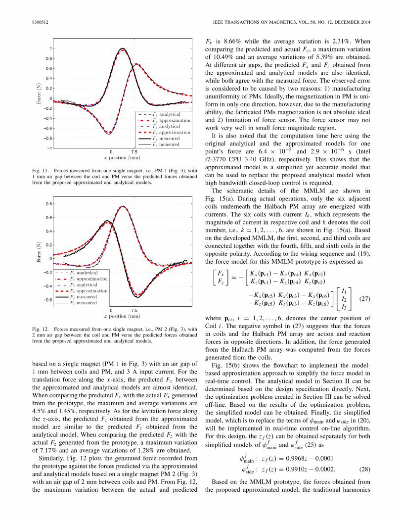
Fig. 11. Forces measured from one single magnet, i.e., PM 1 (Fig. 3), with1 mm air gap between the coil and PM verse the predicted forces obtainedfrom the proposed approximated and analytical models.
Fig. 12. Forces measured from one single magnet, i.e., PM 2 (Fig. 3), with2 mm air gap between the coil and PM verse the predicted forces obtainedfrom the proposed approximated and analytical models.
based on a single magnet (PM 1 in Fig. 3) with an air gap of1 mm between coils and PM, and 3 A input current. For thetranslation force along the x-axis, the predicted Fx betweenthe approximated and analytical models are almost identical.When comparing the predicted Fx with the actual Fx generatedfrom the prototype, the maximum and average variations are4.5% and 1.45%, respectively. As for the levitation force alongthe z-axis, the predicted Fz obtained from the approximatedmodel are similar to the predicted Fz obtained from theanalytical model. When comparing the predicted Fz with theactual Fz generated from the prototype, a maximum variationof 7.17% and an average variations of 1.28% are obtained.
Similarly, Fig. 12 plots the generated force recorded fromthe prototype against the forces predicted via the approximatedand analytical models based on a single magnet PM 2 (Fig. 3)with an air gap of 2 mm between coils and PM. From Fig. 12,the maximum variation between the actual and predicted
Fx is 8.66% while the average variation is 2.31%. Whencomparing the predicted and actual Fz , a maximum variationof 10.49% and an average variations of 5.39% are obtained.At different air gaps, the predicted Fx and Fz obtained fromthe approximated and analytical models are also identical,while both agree with the measured force. The observed erroris considered to be caused by two reasons: 1) manufacturingununiformity of PMs. Ideally, the magnetization in PM is uni-form in only one direction, however, due to the manufacturingability, the fabricated PMs magnetization is not absolute idealand 2) limitation of force sensor. The force sensor may notwork very well in small force magnitude region.
It is also noted that the computation time here using theoriginal analytical and the approximated models for onepoint’s force are 6.4 × 10⁻⁵ and 2.9 × 10⁻⁶ s (Inteli7-3770 CPU 3.40 GHz), respectively. This shows that theapproximated model is a simplified yet accurate model thatcan be used to replace the proposed analytical model whenhigh bandwidth closed-loop control is required.
The schematic details of the MMLM are shown inFig. 15(a). During actual operations, only the six adjacentcoils underneath the Halbach PM array are energized withcurrents. The six coils with current Ik , which represents themagnitude of current in respective coil and k denotes the coilnumber, i.e., k = 1, 2, . . . , 6, are shown in Fig. 15(a). Basedon the developed MMLM, the first, second, and third coils areconnected together with the fourth, fifth, and sixth coils in theopposite polarity. According to the wiring sequence and (19),the force model for this MMLM prototype is expressed as[
where pci , i = 1, 2, . . . , 6, denotes the center position ofCoil i . The negative symbol in (27) suggests that the forcesin coils and the Halbach PM array are action and reactionforces in opposite directions. In addition, the force generatedfrom the Halbach PM array was computed from the forcesgenerated from the coils.
Fig. 15(b) shows the flowchart to implement the model-based approximation approach to simplify the force model inreal-time control. The analytical model in Section II can bedetermined based on the design specification directly. Next,the optimization problem created in Section III can be solvedoff-line. Based on the results of the optimization problem,the simplified model can be obtained. Finally, the simplifiedmodel, which is to replace the terms of φmain and ϕside in (20),will be implemented in real-time control on-line algorithm.For this design, the z f (z) can be obtained separately for bothsimplified models of φ
fmain and ϕ
fside (25) as
φf
main : z f (z) = 0.9968z − 0.0001
ϕf
side : z f (z) = 0.9910z − 0.0002. (28)
Based on the MMLM prototype, the forces obtained fromthe proposed approximated model, the traditional harmonics
TEO et al.: MODELING OF A 2 DoF MMLM 8300512
Fig. 13. Forces measured from the MMLM prototype with 1 mm air gapbetween the coil and PM verse the predicted forces obtained from the proposedand harmonic models.
Fig. 14. Forces measured from the MMLM prototype with 2 mm air gapbetween the coil and PM verse the predicted forces obtained from the proposedand harmonic models.
model, and the experimental measurements are plotted inFigs. 13 and 14, with air gaps of 1 and 2 mm betweenthe PM and coil arrays, respectively. From Fig. 13, themaximum variation between the actual Fx and predicted Fx
obtained from the proposed approximated model is 6.48%while the average variation is 2.30%. When comparing theactual Fz against the predicted Fz obtained via the proposedapproximated model, a maximum variation of 10.22% and anaverage variations of 3.54% are obtained. On the other hand,the maximum variation between the actual Fx and predictedFx obtained from the traditional harmonics model is 79.93%while the average variation is 32%. In addition, the maximumand average variations between the actual Fz and predictedFz obtained from the traditional harmonics model are 128.59%and 49.49%, respectively.
From Fig. 14, the maximum variation between the actualFx obtained from the prototype with 2 mm air gap and
Fig. 15. (a) Schematic details of the MMLM prototype with a moving trans-lator. (b) Flowchart of model implementation in real-time control applications.
predicted Fx obtained from the proposed approximated modelis 7.21%, and the average variation is 2.44%. When comparedagainst the actual Fz , the predicted Fz obtained from theproposed approximated model has a maximum and averagevariations of 12.17% and 4.51%, respectively. As for thepredicted Fx obtained from the traditional harmonics model,a maximum variation of 78.86% and the average variation of32.45% are obtained when compared against the actual Fx .In addition, the maximum and average variations betweenthe actual Fz and predicted Fz obtained from the traditionalharmonics model are 131.68%, and 49.59%, respectively. Theresults obtained from these investigations suggest that theaccuracy of the approximated model in predicting the current–force characteristic of the MMLM prototype with a singlemagnetic pole Halbach PM array is consistent even at differentair gaps.
B. MMLM With Six Magnetic Poles Halbach PM Array
To demonstrate the generality of the proposed models,a separate translator formed by six magnetic poles Halbach PMarray [Fig. 8(c)] was also fabricated to evaluate the accuracyof the proposed magnetic field and force models. First, themagnetic flux density along the x- and z-axis was measured,and Figs. 16 and 17 plot the Bz and Bx of the six magneticpoles PM array obtained experimentally and analytically viathe harmonic and proposed models at air gaps of 5 and 3.5 mm,respectively. When comparing the Bz predicted by the tradi-tional harmonic model and the measured values, the maximumand average variations are 29.89% and 5.04%, respectively.Between the Bx predicted by the traditional harmonic modeland the measured values, a maximum variation of 32.13% andan average variation of 6.35% are obtained. Results show thatthe harmonic field model is effective in predicting the magneticfield of multiple magnetic poles Halbach PM array.
When comparing between the Bz predicted by theproposed magnetic field model and the measured values,a maximum variation of 4.82% and an average variation of
8300512 IEEE TRANSACTIONS ON MAGNETICS, VOL. 50, NO. 12, DECEMBER 2014
Fig. 16. Bz measured from a six magnetic pole Halbach PM array prototypeverse the predicted Bz obtained from the harmonics and proposed modelswith 5 mm air gap.
Fig. 17. Bx measured from a six magnetic pole Halbach PM array prototypeverse the predicted Bz obtained from the harmonics and proposed models with3.5 mm air gap.
2.03% are obtained. Between the Bx predicted by the proposedmagnetic field model and the measured values, the maximumand average variations are 8.28% and 4.01%, respectively.These comparisons show that the proposed magnetic fieldmodel is also able to predict the magnetic field accuratelyeven for multiple magnetic poles Halbach PM array. Therefore,this investigation shows that the proposed magnetic fieldmodel is an effective and generic solution for analyzing aHalbach PM array regardless of the numbers of magneticpoles.
Finally, the forces along the x- and z-axis generated fromthe MMLM prototype with a six magnetic poles HalbachPM array at 0.5 mm air gap were measured and plottedagainst the analytical models in Figs. 18 and 19, respectively.From Fig. 18, the maximum variation between the actual
Fig. 18. Forces along the x-axis measured from the MMLM prototype witha six magnetic poles Halbach PM array at 0.5 mm air gap verse the predictedforces obtained from the proposed and harmonic models.
Fig. 19. Forces along the z-axis measured from the MMLM prototype witha six magnetic poles Halbach PM array at 0.5 mm air gap verse the predictedforces obtained from the proposed and harmonic models.
and predicted Fx obtained from the proposed approximatedmodel is 6.27% while the average variation is 3.19%. Onthe other hand, the maximum and average variations betweenthe actual and predicted Fx obtained from the traditionalharmonics model are 30.99% and 5.63%, respectively. Basedon Fig. 19, the maximum variation between the actual andpredicted Fz obtained from the proposed approximated modelis 12.01% while the average variation is 5.23%. The maximumvariation between the actual and predicted Fz obtained fromthe traditional harmonics model is 45.87% while the aver-age variation is 7.42%. Therefore, this investigation showsthat the proposed approximated model is more accuratein predicting the current–force relationship of a MMLMeven for translator with multiple magnetic poles HalbachPM array.
TEO et al.: MODELING OF A 2 DoF MMLM 8300512
V. CONCLUSION
This paper presents an analytical force modeling approachthat accurately predicts the current–force characteristic of the2 DoF MMLM. Unlike existing theoretical force models, theuniqueness of this model is that it accounts for the flux leakageat the edges of the Halbach PM array, due to a proposedmagnetic field model. Therefore, the proposed model issuitable for both low- and high-order Halbach PM array.Especially for the MMLM with low-order Halbach PM array,the resulted Maglev positioners become smaller and lighter,comparing with existing designs. Furthermore, the proposedmodel is also applicable for Halbach PM arrays with noniden-tical width and height in single PM, this additionally increasethe design freedom for some specific applications.
The proposed magnetic field model for Halbach PM arrayis formulated based on the magnetic current model. Subse-quently, an analytical force model was derived from the mag-netic field model via the Lorentz-force principle. To facilitatethe high sampling rate control applications, an approximationapproach was used to obtain an approximated model, whichis a simplified mathematical representation of the proposedanalytical force model. This approximated model reducesthe computational time and complexity while guarantees theaccuracy of the predicted current–force characteristic of anMMLM. MMLM prototype was developed with translatorswith both single and six magnetic poles Halbach PM arrays.Experimental investigations have shown that the proposedmagnetic field and force models are accurate in predicting themagnetic field and force for both the Halbach PM arrays.
ACKNOWLEDGMENT
This work was supported in part by the Collabora-tive Research Project under the SIMTech-NUS Joint Lab-oratory (Precision Motion Systems), Ref: U12-R-024JL,and in part by SingaporeMOE AcRF Tier 1 under GrantR-263-000-A44-112.
REFERENCES
[1] D. L. Trumper, W.-J. Kim, and M. E. Williams, “Design and analysisframework for linear permanent-magnet machines,” IEEE Trans. Ind.Appl., vol. 32, no. 2, pp. 371–379, Mar. 1996.
[2] W. J. Kim, “High-precision planar magnetic levitation,” Ph.D.dissertation, Dept. Mech. Eng., Massachusetts Inst. Technology, Cam-bridge, MA, USA, 1997.
[3] M. E. Williams, “Precision six degree of freedom magnetically-levitatedphotolithography stage,” Ph.D. dissertation, Dept. Mech. Eng., Massa-chusetts Inst. Technology, Cambridge, MA, USA, 1997.
[4] R. J. Hocken, D. L. Trumper, and C. Wang, “Dynamics and controlof the UNCC/MIT sub-atomic measuring machine,” CIRP Ann., Manuf.Technol., vol. 50, no. 1, pp. 373–376, 2001.
[5] R. Fesperman et al., “Multi-scale alignment and positioningsystem—MAPS,” Precision Eng., vol. 36, no. 4, pp. 517–537,Oct. 2012.
[6] X. Lu and I.-U.-R. Usman, “6D direct-drive technology for planarmotion stages,” CIRP Ann., Manuf. Technol., vol. 61, no. 1, pp. 359–362,2012.
[7] H. Ohsaki and Y. Ueda, “Numerical simulation of mover motion ofa surface motor using Halbach permanent magnets,” in Proc. Int.Symp. Power Electron., Elect. Drives, Autom. Motion, Taormina, Italy,May 2006, pp. 364–367.
[8] J. de Boeij, E. Lomonova, and A. Vandenput, “Modeling ironlesspermanent-magnet planar actuator structures,” IEEE Trans. Magn.,vol. 42, no. 8, pp. 2009–2016, Aug. 2006.
[9] J. W. Jansen, C. M. M. van Lierop, E. A. Lomonova, andA. J. A. Vandenput, “Modeling of magnetically levitated planar actuatorswith moving magnets,” IEEE Trans. Magn., vol. 43, no. 1, pp. 15–25,Jan. 2007.
[10] C. M. M. van Lierop, J. W. Jansen, A. A. H. Damen, E. A. Lomonova,P. P. J. van den Bosch, and A. J. A. Vandenput, “Model-based com-mutation of a long-stroke magnetically levitated linear actuator,” IEEETrans. Ind. Appl., vol. 45, no. 6, pp. 1982–1990, Nov./Dec. 2009.
[11] H.-S. Cho, C.-H. Im, and H.-K. Jung, “Magnetic field analysis of 2-Dpermanent magnet array for planar motor,” IEEE Trans. Magn., vol. 37,no. 5, pp. 3762–3766, Sep. 2001.
[12] W. Min et al., “Analysis and optimization of a new 2-D magnet arrayfor planar motor,” IEEE Trans. Magn., vol. 46, no. 5, pp. 1167–1171,May 2010.
[13] J. Peng and Y. Zhou, “Modeling and analysis of a new 2-D Halbach arrayfor magnetically levitated planar motor,” IEEE Trans. Magn., vol. 49,no. 1, pp. 618–627, Jan. 2013.
[14] P. Berkelman and M. Dzadovsky, “Magnetic levitation over large trans-lation and rotation ranges in all directions,” IEEE Trans. Mechatronics,vol. 18, no. 1, pp. 44–52, Feb. 2013.
[15] Q. Xu, “Design and development of a flexure-based dual-stage nanopo-sitioning system with minimum interference behavior,” IEEE Trans.Autom. Sci. Eng., vol. 9, no. 3, pp. 554–563, Jul. 2012.
[16] L. Wang, J. Zheng, and M. Fu, “Optimal preview control of dual-stageactuators system for triangular reference tracking,” in Proc. 10th IEEEInt. Conf. Control Autom. (ICCA), Jun. 2013, pp. 164–169.
[17] I. J. C. Compter, “Electro-dynamic planar motor,” Precision Eng.,vol. 28, no. 2, pp. 171–180, Apr. 2004.
[18] H. Jiang, X. Huang, G. Zhou, Y. Wang, and Z. Wang, “Analytical forcecalculations for high-precision planar actuator with Halbach magnetarray,” IEEE Trans. Magn., vol. 45, no. 10, pp. 4543–4546, Oct. 2009.
[19] T. J. Teo, I.-M. Chen, G. Yang, and W. Lin, “Magnetic field model-ing of a dual-magnet configuration,” J. Appl. Phys., vol. 102, no. 7,pp. 074924-1–074924-12, 2007.
[20] E. P. Furlani, Permanent Magnet and Electromechanical Devices.New York, NY, USA: Academic, 2001.
[21] M.-Y. Chen, T.-B. Lin, S.-K. Hung, and L.-C. Fu, “Design and experi-ment of a macro–micro planar maglev positioning system,” IEEE Trans.Ind. Electron., vol. 59, no. 11, pp. 4128–4139, Nov. 2012.
Tat Joo Teo (M’09) received the B.Eng. (Hons.) degree in mechatronicsengineering from the Queensland University of Technology, Brisbane, QLD,Australia, in 2003, and the Ph.D. degree in mechanical and aerospaceengineering from Nanyang Technological University, Singapore, in 2009.
He joined the Singapore Institute of Manufacturing Technology, Singa-pore, in 2009, as a Researcher with the Mechatronics Group. He holdsfour patents granted and two provisional patents filed. His current researchinterests include ultraprecision system, compliant mechanism theory, parallelkinematics, electromagnetism, electromechanical system, thermal modelingand analysis, energy-efficient machine, and topological optimization.
Dr. Teo serves as a Technical Reviewer of the IEEE TRANSACTIONS ONMECHATRONICS; the IEEE TRANSACTIONS ON ROBOTICS, MECHANISM,AND MACHINE THEORY; and IFAC Mechatronics Journal. He was a recipientof the Best Session Paper Award in the 39th Annual Conference of the IEEEIndustrial Electronics Society in 2013. One of his patents was selected as therecipient of 2014 R&D 100 Award.
Haiyue Zhu (S’13) received the B.Eng. degree in automation from theSchool of Electrical Engineering and Automation and the B. Mgt. degreein business administration from the College of Management and Economics,Tianjin University, Tianjin, China, in 2010, and the M.Sc. degree in electricalengineering from the National University of Singapore (NUS), Singapore, in2013, where he is currently pursuing the Ph.D. degree with the Departmentof Electrical and Computer Engineering.
He joined the Singapore Institute of Manufacturing Technology (SIMTech)-NUS Joint Laboratory on Precision Motion Systems in 2013, and isan Attached Research Student with the Agency for Science, Technology,and Research, SIMTech. His current research interests include integratedservo-mechanical design of precision mechatronics and magnetic levitationtechnology.
8300512 IEEE TRANSACTIONS ON MAGNETICS, VOL. 50, NO. 12, DECEMBER 2014
Chee Khiang Pang (Justin) (S’04–M’07–SM’11) received the B.Eng.(Hons.), M.Eng., and Ph.D. degrees in electrical and computer engineeringfrom the National University of Singapore (NUS), Singapore, in 2001, 2003,and 2007, respectively.
He was a Visiting Fellow with the School of Information Technologyand Electrical Engineering (ITEE), University of Queensland (UQ), Brisbane,QLD, Australia, in 2003. From 2006 to 2008, he was a Researcher (Tenure)with Central Research Laboratory, Hitachi Ltd., Tokyo, Japan. In 2007, hewas a Visiting Academic with the School of ITEE. From 2008 to 2009,he was a Visiting Research Professor with the Automation and RoboticsResearch Institute, University of Texas at Arlington, Fort Worth, TX, USA.He is currently an Assistant Professor with the Department of Electrical andComputer Engineering at NUS. He is also an Associate with the Agencyfor Science, Technology, and Research (A*STAR), Singapore Institute ofManufacturing Technology, and a Faculty Associate with the A*STAR DataStorage Institute. He has authored and edited three research monographs,Intelligent Diagnosis and Prognosis of Industrial Networked Systems (CRCPress, 2011), High-Speed Precision Motion Control (CRC Press, 2011),and Advances in High-Performance Motion Control of Mechatronic Systems
(CRC Press, 2013). His research interests are on ultra-high performancemechatronic systems, with specific focus on advanced motion control fornanopositioning systems, precognitive maintenance using intelligent analytics,and energy-efficient task scheduling considering uncertainties
Dr. Pang is a Member of the American Society of Mechanical Engineers.He is currently serving as an Associate Editor of the Journal of DefenseModeling and Simulation and Transactions of the Institute of Measurementand Control; on the editorial board of the International Journal of AdvancedRobotic Systems, the International Journal of Automation and Logistics,and the International Journal of Computational Intelligence Research andApplications; and on the conference editorial board of the IEEE ControlSystems Society. In recent years, he also served as a Guest Editor of the AsianJournal of Control, the International Journal of Systems Science, the Journalof Control Theory and Applications, and the Transactions of the Institute ofMeasurement and Control. He was a recipient of the Best Application PaperAward at the 8th Asian Control Conference, Kaohsiung, Taiwan, in 2011,and the Best Paper Award at the International Association of Science andTechnology for Development, International Conference on Engineering andApplied Science, Colombo, Sri Lanka, in 2012.


![A novel six-degrees-of-freedom series-parallel … · A novel six-degrees-of-freedom series-parallel manipulator ... Kutzbach criterion [19], is capable to realize six degrees of](https://static.documents.pub/doc/80x56/5b79f3c77f8b9a703b8ebdd5/a-novel-six-degrees-of-freedom-series-parallel-a-novel-six-degrees-of-freedom.jpg)


