Page 1
MODELING OF BIOPOLYMERIZATION PROCESS USING FIRST
PRINCIPLE MODEL AND BOOTSTRAP RE-SAMPLING
NEURAL NETWORK
RABIATUL ‘ADAWIAH BINTI MAT NOOR
UNIVERSITI SAINS MALAYSIA
2011
brought to you by COREView metadata, citation and similar papers at core.ac.uk
provided by Repository@USM
Page 2
ii
ACKNOWLEDMENTS
“In the name of Allah, The Most Gracious, The Most Merciful”
First and foremost, I would like to express my humble gratitude to GOD for He is the
only one to make it possible for me to finish my research and have my thesis done.
My utmost thank you goes to my parents and my family who always encourage me
to achieve whatever that I want to do in life, the one that always support me with
their guidance and affection. For the Dean and Deputy Dean of School of Chemical
Engineering (SCE), thank you for all your support and guidance. My unfathomable
appreciation and gratitude also goes to my supervisor, Dr. Zainal Ahmad. I am really
grateful to have such an understanding, helpful yet fun supervisor such as you. Apart
for being my guru who taught to me about how to be a postgraduate student and
conduct my research, you are also my best friend who is always be there for me
through thick and thin. To my co-supervisor, Associate Professor Dr. Mashitah Mat
Don, you are the one to look up for having such a strong will and very hardworking
as a woman. As for Dr. Mohamad Hekarl Uzir, thank you so much for being my
biochemical engineer and mathematician. To Dr. Khairiah Abd. Karim, thank you so
much for allowing me to use space in your laboratory. I really appreciate it. For the
administrative and technical staffs, I have no words to say how much I appreciate all
your help and support. To all USM’s SCE staffs, thank you for making me feel like I
am part of this amazing family. Not to forget MOSTI for the fund through
Sciencefund Grant No. 6013336, RU FRGS Grant No. 811106 and all my comrades
in SCE. Thank you all. May God bless all of you.
Page 3
iii
TABLE OF CONTENTS
ACKNOWLEDGEMENTS ii
TABLE OF CONTENTS iii
LIST OF TABLES viii
LIST OF FIGURES ix
LIST OF PLATES xiii
LIST OF ABBREVIATIONS xiv
LIST OF SYMBOLS xvii
LIST OF SCHEMES xix
ABSTRAK xx
ABSTRACT xxii
CHAPTER ONE: INTRODUCTION
1.0 Research Background 1
1.1 Problem Statement 8
1.2 Research Objectives 9
1.3 Organization of Thesis 10
CHAPTER TWO: LITERATURE REVIEW
2.0 Introduction 12
2.1 Types of Neural Networks 18
2.2 Feedforward Artificial Neural Network (FANN) 21
2.2.1 Training Paradigms in Feedfoward Neural Network 23
2.2.2 Levenberg-Marquardt Training Paradigm 25
Page 4
iv
2.3 Improvements in Neural Network Modeling 27
2.3.1 Bootstrap Re-sampling Neural Networks 27
2.3.2 Stacked Neural Networks 29
2.4 Types of Model 32
2.5 Feedforward Artificial Neural network (FANN) Applications in 33
Modeling of Polymerization Processes
2.5.1 Neural Network in Prediction of Polymer Quality 33
2.5.2 Bootstrap and Stacked Neural Network in Modeling and 36
Control of Polymerization Process
2.5.3 Neural Network as Hybrid Model 44
2.5.4 Neural Network as Universal Modeling Tool 50
2.6 Biopolymerization of Lactones to Polyester 60
2.7 Advantages of Enzyme-Catalyzed Polymerization 62
2.8 Ring-Opening Polymerization of -Caprolactone (-CL) 63
2.9 Biopolymer Quality 66
2.10 Modeling of Biopolymerization Process Using First Principle Model 67
2.11 Conclusion on Literature Review 69
CHAPTER THREE: MATERIALS AND METHODS FOR EXPERIMENTS
3.0 Introduction 70
3.1 Chemicals 70
3.2 Equipments 72
3.3 Experimental Procedures 75
3.4 Analytical Methods 79
Page 5
v
3.4.1 Gel Permeation Chromatograph (GPC) Analysis 79
3.4.2 Gas Chromatograph (GC) Analysis 81
CHAPTER FOUR: PROCESS MODELING FIRST PRINCIPLE AND
EMPIRICAL MODEL
4.0 Introduction 85
4.1 Development of Process Model - First Principle Model 86
4.1.1 Enzymes – Catalysts and Kinetics 87
4.1.2 The Briggs-Haldane Steady-State Approach 93
4.1.3 Deriving Differential Equations from Reversible Reaction –
Briggs and Haldane Perspectives 95
4.1.4 Enzyme-Catalyzed System – A Dynamic Analysis 99
4.1.5 Mechanism of Lipase-Catalyzed Ring Opening
Polymerization (ROP) Reaction 102
4.1.6 Development of the Model – Case Study: Biopolymerization
of -Caprolactone to Polycaprolactone 103
4.1.7 Determining k Values in Ordinary Differential Equations 107
4.1.8 Verification of First Principle Model 113
4.2 Development of Process Model Based on Empirical Model 112
4.2.1 Data Generation for Empirical Model 114
4.2.2 Data Scaling for Empirical Model 115
4.2.3 Selection of Input-Output for Empirical Model 116
4.2.4 Selecting Number of Hidden Layers for Empirical Model 117
Page 6
vi
4.2.5 Choosing Number of Hidden Neurons 118
4.2.6 Weight, Bias and Activation Function 119
4.2.7 Neural Network – Static and Dynamic Model 119
CHAPTER FIVE: RESULTS AND DISCUSSION
5.0 Introduction 121
5.1 Biopolymerization Process Modeling – Empirical Model Perspective 121
5.1.1 Biopolymerization Process Modeling – Flask Level 122
5.1.2 Biopolymerization Process Modeling – Reactor Level 126
5.2 Biopolymerization Process Modeling – First Principle Model
Perspective 129
5.3 Results Analysis and Discussion 134
CHAPTER SIX: CONCLUSIONS AND RECOMMENDATIONS FOR
FUTURE STUDIES
6.0 Conclusions 142
6.1 Recommendations for Future Studies 144
REFERENCES 146
APPENDICES 162
Page 7
vii
Appendix A 162
Appendix B 172
Appendix C 175
LIST OF PUBLICATIONS 181
Page 8
viii
LIST OF TABLES
Page
Table 2.1 Biological-Artificial Neuron Analogy 14
Table 4.1 Methods for Approximating 𝐾𝑚 and 𝑉𝑚𝑎𝑥 93
Table 5.1 Numerical Analysis of Bootstrap Neural Network Model
for Flask Level 125
Table 5.2 Numerical Analysis of Bootstrap Neural Network Model 128
for Reactor Level
Table 5.3 p-value from ANOVA for Each Batch of Reaction 135
Page 9
ix
LIST OF FIGURES
Page
Figure 1.1 A Simplified Flowchart of the Whole Research Work 7
Figure 2.1 (a) Biological Neuron; (b) Artificial Neural Network
Representation 15
Figure 2.2 Biological Neuron Elements-Artificial Neural Network
Elements Comparison 17
Figure 2.3 A Simplified Kohonen Network 20
Figure 2.4 A Multi-layer Feedforward Neural Network 22
Figure 2.5 Basic Neural Network Training Method 24
Figure 2.6 The Analogy Of Bootstrap Re-Sampling Technique:
(a) Data samples in the original data set
(b) Data samples in the re-sampled data set 28
Figure 2.7 A Stacked Neural Network 29
Figure 2.8 The Structure of the Neural-Fuzzy Model of the
Polymerization Process 35
Figure 2.9 Schematic Diagram of Hybrid Neural-Network
Rate-Function (HNNRF) Model 47
Figure 2.10 Direct Inverse Control Strategies with Hybrid Neural
Page 10
x
Network (HNN) Inverse Model as Controller 50
Figure 2.11 Structures of Neural Networks with 7 Nodes in the Input 51
Figure 2.12 A Simplified Biopolymerization of ε-Caprolactone to
Poycaprolactone Reaction 64
Figure 2.13 Candida antarctica lipase B Structure 66
Figure 3.1 Schematic Diagram of the Bioreactor System 75
Figure 3.2 Schematic Diagram of Gel Permeation Chromatograph
(GPC) System 80
Figure 3.3 Schematic Diagram of Gas Chromatograph (GC) System 82
Figure 3.4 Flowchart of the Experimental Works 83
Figure 4.1 Reaction Coordinate Diagram of Uncatalyzed and
Catalyzed Reaction 88
Figure 4.2 Progress Curves of an Enzyme-Catalyzed Reaction
with Time 90
Figure 4.3 Development of First Principle Model for Enzymatic
System 100
Figure 4.4 Calibration Curve for Residual Monomer Analysis 108
Figure 4.5 The Plot of 1/v vs. 1/[M] 109
Figure 4.6 Development of First Principle Model for
Page 11
xi
Biopolymerization Process 111
Figure 4.7 Monomer (Substrate)-Polymer Concentration Plot from
First Principle Model 112
Figure 4.8 Development Bootstrap Re-Sampling Neural Network
Technique 114
Figure 4.9 Relationship between Input-Output of Neural Network
Model 117
Figure 5.1 Bootstrap Neural Network Model Performance on
Training and Testing Process (Flask Level) 123
Figure 5.2 Bootstrap Neural Network Model Performance on
Validation Process (Flask Level) 124
Figure 5.3 Model Residue for Validation Data (Flask Level) 124
Figure 5.4 Bootstrap Neural Network Model Performance on
Training and Testing Process (Reactor Level) 127
Figure 5.5 Bootstrap Neural Network Model Performance on
Validation Process (Reactor Level) 127
Figure 5.6 Model Residue for Validation Data (Reactor Level) 128
Figure 5.7 Biopolymer Molecular Weight for Flask, Reactor and
First Principle Model For 50 C 131
Page 12
xii
Figure 5.8 Biopolymer Weight for Flask, Reactor and
First Principle Model For 60 C 131
Figure 5.9 Biopolymer Weight for Flask, Reactor and
First Principle Model For 70 C 132
Figure 5.10 Biopolymer Weight for Flask, Reactor and
First Principle Model For 80 C 132
Figure 5.11 Biopolymer Weight for Flask, Reactor and
First Principle Model For 90 C 133
Figure 5.12 Biopolymer Weight for Flask, Reactor and
First Principle Model For 100 C 133
Figure 5.13 Box Plot for Molecular Weight at Reaction
Temperature 50 C 139
Figure 5.14 Box Plot for Molecular Weight at Reaction
Temperature 60 C 139
Figure 5.15 Box Plot for Molecular Weight at Reaction
Temperature 70 C 140
Figure 5.16 Box Plot for Molecular Weight at Reaction
Temperature 80 C 140
Figure 5.17 Box Plot for Molecular Weight at Reaction
Page 13
xiii
Temperature 90 C 141
Figure 5.18 Box Plot for Molecular Weight at Reaction
Temperature 100 C 141
LIST OF PLATES
Plate 3.1 The Bioreactor for Biopolymerization Process of
ε-Caprolactone 73
Plate 3.2 The Bioreactor System for Biopoymerization of
ε-Caprolactone 73
Page 14
xiv
LIST OF ABBREVIATIONS
ε-CL Epsilon Caprolactone
ACS American Chemical Society
ANN Arficial neural network
ANN-SS Artificial neural network-soft sensor
ANOVA Analysis of variance
ART Adaptive resonance theory
BAGNET Bootstrap aggregated network
BP Backpropagation
CAL-B Candida antarctica Lipase B
CSTR Continuous stirred tank reactor
EKF Extended Kalman filter
FDA Foods and Drugs Administration
FFN Feed forward network
FID Free inductive detector
GC Gas chromatograph
GPC Gel permeation chromatograph
HNN Hybrid neural network
HNNRF Hybrid neural network rate function
HPLC High performance liquid chromatograph
IRN Internal recurrent network
LM Levenberg-Marquardt
MISO Multiple input single ouput
MLP Multi-layer perceptron
MLR Multiple linear regression
Page 15
xv
MLRN Multi-layer recurrent network
MMA Methyl methacrylate
MPC Model predictive control
MW Monomer molecular weight
NMAX Nonlinear moving average with exogenous inputs
NMAX-MLRN Nonlinear moving average with exogenous inputs multi-layer
recurrent network
NMAX-RTRL Nonlinear moving average with exogenous inputs real time
real learning
NNMPC Neural network model predictive control
NNRF Neural network rate function
PCL Polycaprolactone
PCR Principal component regression
PDF Probability density function
PI Proportional-Integral
PID Proportional-Integral-Derivative
PRMS Pseudo random multi-state signal
R Correlation coefficient
RMSE Root mean squared error
RNN Recurrent neural network
ROP Ring-opening polymerization
RTRL Real time real learning
SISO Single input single output
SPUD Sequential pseudo-uniform design
SSE Sum squared error
Page 16
xvi
THF Tetrahydrofuran
USEPA United States Environmental Protection Agency
VA Vinyl acetate
VLE Vapor-liquid equilibrium
VLSI Very large scale integration
Page 17
xvii
LIST OF SYMBOLS
k1,…, k3 Forward rate constant mol/s, s-1
k-1,…, k-3 Reverse rate constant mol/s,s-1
Unit
𝜎 Transfer function -
𝛼 Significance level -
E Energy function -
N Total number of nodes -
G Free energy Joule
[S] Substrate concentration mol/cm3
[P] Product/biopolymer concentration mol/cm3
[E] Enzyme concentration mol/cm3
[ES] Enzyme-substrate complex -
[M] Monomer concentration mol/cm3
[EM] Enzyme-monomer complex -
[HA] -hydroxy carboxylic acid mol/cm3
[E]T Total enzyme concentration mol/cm3
[P]eq Equilibrium product concentration mol/cm3
[S]eq Equilibrium substrate concentration mol/cm3
[M]o Initial monomer concentration mol/cm3
hj Hidden layer output -
H0A Null hypothesis for all samples from factor A -
H0B Null hypothesis for all samples from factor B -
ki Rate constant of particular pathway mol/s, s-1
Page 18
xviii
Keq Equilibrium rate constant -
Km Michaelis-Menten constant mol/cm3
KmM Monomer Michealis-Menten constant mol/cm3
KmP Polymer Michaelis-Menten constant mol/cm3
kp Rate constant for the breakdown of ES to E + P mol/s, s-1
Mn Number-average molecular weight g/mol
Mw Weight-average molecular weight g/mol
uj Hidden layer weighted sum -
v Velocity min-1
vj Output layer weighted sum -
Vr Reverse velocity min-1
Vf Forward velocity min-1
Vmax Maximum velocity min-1
Vmaxf Maximum forward velocity min-1
wji Hidden layer weight -
wkj Output layer weight -
yk Output layer output -
(x1,…,xp) Vector of predictor variable value -
𝑑 𝑆
𝑑𝑡
𝑑 𝑀
𝑑𝑡
Rate of substrate/monomer concentration over
time
-
𝑑 𝐸𝑆
𝑑𝑡
𝑑 𝐸𝑀
𝑑𝑡
Rate of enzyme-substrate concentration over
time
-
𝑑 𝐻𝐴
𝑑𝑡
Rate of concentration over time -
𝑑 𝑃
𝑑𝑡
Rate of polymer/product concentration over time -
Page 20
xix
LIST OF SCHEMES
Page
Scheme 4.1 Mechanism of Ring Opening Polymerization of Lactones 102
Page 21
xx
PERMODELAN PROSES BIOPOLIMERISASI MENGGUNAKAN MODEL
PRINSIP PERTAMA DAN JARINGAN NEURAL PERSAMPELAN SEMULA
IKAT BUT
ABSTRAK
Kemunculan isu alam sekitar seperti kesan rumah hijau dan pemanasan global telah
mencetuskan idea bagi para pengkaji dan saintis untuk mencipta bahan baru yang
mampu menangani isu alam sekitar dan sekaligus memenuhi kehendak manusia iaitu
biopolimer. Kualiti biopolimer adalah dinilai melalui berat molekulnya. Sehingga
kini tiada pengukuran atas talian bagi berat molekul polimer. Oleh itu, kajian ini
membangunkan model untuk menyerupai proses sebenar dengan menggunakan
kaedah permodelan seperti jaringan neural. Model prinsip pertama juga telah menjadi
antara kaedah paling digunakan untuk membangunkan model selain dari
menggunakan kaedah permodelan seperti jaringan neural. Jadi, jaringan neural dan
model prinsip pertama telah digunakan dalam untuk membangunkan model process
biopolimerirasi dan keputusan bagi kedua-dua model ini dibandingkan. Bagi
membangunkan model-model ini, eksperimen dijalankan untuk mendapatkan data
untuk kedua-dua model. Data bagi model jaringan neural adalah berat molekul
biopolimer manakala data bagi model prinsip pertama adalah data kinetik. Kedua-
dua model menggunakan pendekatan berlainan iaitu pendekatan secara teori dan
empirikal. Kedua-dua model juga memberikan keputusan yang baik dari segi nombor
berat molekul mahupun trendnya. Berdasarkan keputusan dari kedua-dua model,
model jaringan neural memberikan keputusan terbaik dengan ralat jumlah kuasa dua
sebanyak 0.9996 dan pekali kolerasi sebanyak 0.9999. Model prinsip pertama pula
Page 22
xxi
dinilai berdasarkan analisis varian (ANOVA). Dalam kajian ini, ANOVA mengambil
aras kepentingan, α sebagai 0.01. Oleh itu, keputusan yang memberi nilai kurang dari
0.01 menunjukkan bahawa ianya berbeza dari satu sama lain. Ini adalah situasi yang
tidak dikehendaki kerana keputusan yang baik adalah yang memberi keputusan yang
hampir kepada berat molekul sebenar dari eksperimen. Berdasarkan keputusan
ANOVA, semua keputusan adalah lebih dari 0.01. Ini bermakna keputusan dari
model prinsip pertama adalah hampir sama dengan keputusan dari eksperimen.
Berdasarkan keputusan yang diberi oleh kedua-dua model telah membuktikan
bahawa kedua-dua model adalah kaedah yang tepat dalam membangunkan model
bagi meramal berat molekul biopolimer. Kaedah jaringan neural bagaimanapun telah
memberi keputusan yang lebih baik berbanding model prinsip pertama.
Page 23
xxii
MODELING OF BIOPOLYMERIZATION PROCESS USING FIRST
PRINCIPLE MODEL AND BOOTSTRAP RE-SAMPLING NEURAL
NETWORK
ABSTRACT
The emergence of the environmental issues such as green house and global warming
have triggered scientists and researchers to create new materials that can cope both
environmental and humanity needs i.e. biopolymer. Biopolymer quality assesses by
its molecular weight. Apparently, there is no online measurement for molecular
weight measurement. Therefore, in this study models are developed to mimic the real
process using a reliable modeling tool such as neural networks. First principle model
also become one of the most applied methods to model a process other than using a
modeling tool such as neural network. Therefore in this research, neural network and
first principle model have been chosen to model the biopolymerization process and
followed by the comparison between the aforementioned models. In order to develop
the models, experimental work is conducted to obtain data for first principle model
and neural network model. The data for the neural network model are the molecular
weight of the biopolymer whereas the data for the first principle model are the
kinetics data. Both models delivered predicted molecular weight of biopolymer using
different approaches i.e. fundamental and empirical model. Both models delivered
convincing results in terms of molecular weight number as well as molecular weight
trend. Based on the results from both models, neural network model gives closest
prediction with sum squared error (SSE) is 0.9996 and correlation coefficient, R
value is 0.9999. First principle model results on the hand assessed based on Analysis
Page 24
xxiii
of Variance (ANOVA). In this work, ANOVA takes the significant level, α as 0.01.
Hence, the results that give the value that is less that 0.01, is showing that the
compared data are significantly different from each other which is undesirable as the
actual and predicted data should be projected similar trend and number. According to
the ANOVA for first principle model, all the results are more than 0.01 which mean
that the actual and predicted molecular weights are similar. These results have
proved that both neural network and first principle model are reliable tools in
prediction of molecular weight of biopolymer which neural network model appeared
to be the more precise model in terms of biopolymer molecular weight prediction.
Page 25
1
CHAPTER ONE
INTRODUCTION
1.0 Research Background
The world now has loudly spoken about ‘going green’. One of the ways to
support this manifesto is to utilize biodegradable materials such as biopolymer. One
of the methods to achieve this is by ring opening polymerization process of lactones
to polyester (polycaprolactone) catalyzed by enzyme (lipase) (Kumar and Gross,
2000). Despite of this ambitious goal, the intricacy of polymerization and the
difficult-to-measure variable such as molecular weight have become obstacle us to
achieve an optimum condition of the process and also to produce the desired product
without much waste to be thrown away. Beside the difficulties in measuring and
analyzing the molecular weight of the biopolymer, the biopolymerization process
itself exhibits a very non-linear behavior. Modeling and control of non-linear process
is an uneasy task and requires a powerful and reliable tool to tackle the process. Thus,
artificial intelligent application using neural network model can be said as the
solution of this puzzle (Zhang, 1999; Zhang et al., 2006).
Through a lab-scale reactor with adequate instrumentation, the desired
biopolymerization process can be done and the data retrieved from the experiment is
then used to model the process using neural network. The developed model can be
used to predict the output (molecular weight) of biopolymerization process of
lactones to polyester using lipase as catalyst which can possibly heal our biggest
‘headache’ for analyzing the polymer in order to obtain its molecular weight. The
Page 26
2
good news is that there are many researchers have employed polymerization
processes in their researches and many of them have somehow tried to model the
process in order to mimic chemically catalyzed polymerization process using either
first principle model or empirical model. Even though this work is focusing on
biopolymerization process, it seems that the success of previous works on modeling
chemically catalyzed polymerization process have become proofs that a nonlinear
polymerization process can be modeled using the aforementioned approaches and
have also exhibited convincing results. Such circumstances have shed some light on
this particular process and became a sign that biopolymerization process also can be
modeled using either first principle model or empirical model. All the succeeded
works can be discovered in Chapter 2.
Since half a century ago, researchers have discovered the ultimate tool and
the so-called artificial intelligence to render a new method in order to cope with
processes that require precision and accuracy especially when dealing with a
nonlinear process that unfortunately cannot properly be interpreted mechanistically.
Since the discovery of the tool, researchers have realized that the ‘control targets’
should be able to achieve by using this tool. Neural network has been shown to be
able to approximate any continuous non-linear functions and it has been used to build
data base empirical models for non-linear processes (Hertz, 1991).
Neural network or artificial neural network is said to mimic the human brain
in solving problems. According to Haykin (Haykin, 1994), a neural network is a
massive parallel-distributed processor that has a natural capability for storing
experiential knowledge and making it available for use in the future system. It
resembles the brain in two respects; firstly, the knowledge is acquired by the
Page 27
3
networks through a learning process and secondly, the interneuron connection
strengths known as synaptic weights are used to store the acquired knowledge.
Based on the above observation, neural networks can be said as a remedy to
cope with intricate processes. One of the main advantages of neural network- based
process models is that they are easy to build (Zhang et al., 2006; Zhang, 2008). This
feature is particularly useful when modeling complicated processes where detailed
mechanistic models are difficult to develop. Nonetheless, many researches on neural
networks are mainly focus on feed forward neural networks. This is due the fact that
it is the simplest neural network architecture yet reliable to be applied in various
applications and processes (Zhang et. al, 1999). Therefore, this work has set to focus
more on feed forward neural network. It is just a matter of modification of the neural
network architecture such as single, multiple networks, hybrid, etc. that determine
the performance of the network in each applications. Other neural network
architectures such as recurrent network has received quite a tremendous consent
amongst researchers, however, feed forward neural network is still the most
implemented neural network architecture to date (Gonzaga et al., 2009; Zhang, 2008;
Gomm et al., 1993).
However, a critical shortcoming of all neural networks is that they often lack
robustness, unless a proper network training and validation procedure is used (Zhang
et al., 1999, Zhang, 2009). Robustness of the model can be defined as one of the
baselines to judge the performance of neural network models and it is really related
to the learning or training classes as what Bishop (Bishop, 1995) described in his
work. The importance of neural networks in this context is that they offer very
powerful and general framework to represent non-linear mappings from several input
Page 28
4
variables to several output variables, where the form of the mapping is governed by a
number of adjustable parameters (Gomm et al., 1993).
Many factors can contribute to the success of the neural network
implementations (Hinton, 1992; Haykin, 1994). In particular, neural network is non-
linear models, which are very useful in modeling nonlinear systems that cannot be
successfully modeled by linear models. The second factor is that neural network is
easy to use and develop and they basically learn by examples (Zhang et al., 2006;
Zhang et al., 2008). The neural network users gather representative data, and then
invoke a training algorithm to automatically learn the structure of the data (English,
1996; Chen et al., 1999).
Because of the tremendous capability of neural networks, currently there are
a lot of applications of neural network in industry and business and they are applied
in pattern recognition such as automated recognition of hand-written text, finger print
identification and moving target on a static background (Seong-Wan, 1999; Chen et
al., 1997). Neural networks have also been used in speech production where a neural
network model is connected to a speech synthesizer (Baig et al., 1999; Furlanello et
al., 1999).
Real time control is also a major application of neural networks with neural
network models having been applied in the monitoring and control of complex plants
such as chemical plants (Zhang et al., 1998a; Jazayeri-Rad, 2004). Neural network
has been employed in business where neural network model have played a role in
predicting the stock market trend in certain period of time (Fletcher and Goss, 1993;
Desai and Bharati; 1998). Another area of applications of neural network models is
in signal processing and other typical applications such as noise suppression, filtering
Page 29
5
and digital signal processing technology (Larsson et al., 1996). These broad
applications of neural networks can be a substantiation of the superiority of neural
network. Despite of their advantages, researchers have continuously attempted to
improve neural network to better suit many complex processes.
In order to improve the robustness of neural networks a number of techniques
have been developed lately like regularization (Girosi et al., 1995) and the early
stopping method (Morgan and Bourlard, 1990). Ohbayashi and co-workers
(Ohbayashi et al., 1998) implemented the universal learning rule and second order
derivatives to increase the robustness in neural network models. Robustness is
enhanced by minimizing the change in the values of criterion function caused by the
small changes around the nominal values of system parameters. Lack of the
robustness in individual neural networks is basically due to the overfitting of the
models (Caruana et al., 2000).
Overfitting basically refers to the poor generalization of the networks due to
fitting the noise in the data (Mc Loone and Irwin, 2001). Furthermore, the trained
network might not minimize the error on the training data set because it has
uncontrolled excess dynamics capability or because the training data itself is
corrupted with noise. The representation capability of a neural network is determined
by its size (number of neurons). If networks are too large, they can find many
solutions which exactly fit the training set data but without the presence of the
frequency dynamics in the underlying function. When the data is corrupted with
noise, a second form of overfitting occurs and will result in the networks fitting the
noise (McLoone and Irwin, 2001).
Page 30
6
In order to inhibit all the drawbacks that are mentioned earlier, a modified
neural network that offers better presentation of a model can be developed based on
available method such as bootstrap re-sampling method. Sometimes, a complicated
process may experience problem such as insufficient data. Therefore, bootstrap re-
sampling has been identified to as a method to overcome this problem by re-sample
original data to produce additional data without interfere with the integrity of the data.
Basically, data re-sampling is the act of rearranging the original data to form new
sets of data. It is better known as the bootstrap re-sampling method. Further
discussion about neural networks can be found in Chapter 2.
Figure 1.1 is a pictograph in the form of flowchart can be a simplified way to
convey the whole idea behind this work.
Page 31
7
Figure 1.1: A Simplified Flowchart of the Whole Research Work
To predict/develop
model of biopolymer
molecular weight
Expensive analytical
equipment to analyze
biopolymer
Lack of online measurement
system for measuring biopolymer
molecular weight
Develop a model to mimic the biopolymerization in order
to predict biopolymer molecular weight
(i.e. through experimental works and also fundamental
knowledge of sciences and engineering)
Ubiquitous modeling tool –
Neural network modeling
(bootstrap re-sampling neural network)
Many applications have
utilized biopolymer as the
material of constructions
Biopolymer is biodegradable –
very desirable in green
technology era
The GOAL
The
PROBLEM
The
SOLUTION
The
METHOD
WHY?
Neural network model and
first principle model
successfully predict and
generate biopolymer
molecular weight.
The
RESULTS
First principle model -
biopolymerization
process reaction study
Page 32
8
1.1 Problem Statement
Polymerization process which always classified as a complex process and
also lack of instrumentation which can deliver a fast and accurate measurement of
polymer molecular weight have become the motivation to start this research.
Demanding and fast-growing polymer industries have sent this conventional
measurement scheme over the edge. A truly reliable and trustworthy system for
coping with the intricacy of the polymerization process meanwhile still can guarantee
the highest process safety, the ultimate product quality and also maximum profit is
indeed being a highlight in recent research phenomena. When putting reliability,
simplicity and intricacy as the desirable criteria of the model, neural networks have
emerged as primary choice to bring such criteria into reality.
Moreover, complicated process such as biopolymerization that requires a
long reaction time has resulted to the problem such as insufficient data from the real
process. Such a problem can lead to undesired conditions in neural network modeling
such as underfitting. Besides, measurement for polymer molecular weight also has
caused such a problem where online measurement for polymer molecular weight is
impossible. Most biopolymers are assessed by offline analyzer such as Gel
Permeation Chromatograph (GPC) for their molecular weight. Thus, a tool that can
solve both problems in a model has to be created in order to be able to mimic the real
biopolymerization process. Neural network model has been found to be the most
eligible tool to tackle these problems. With latest computer technology, the model
can be implemented easily. Moreover, neural network also comes with several
improved methods such as bootstrap re-sampling method that can be applied to
generate additional data for training and testing processes.
Page 33
9
Therefore, artificial intelligence (i.e. neural network) has been identified to be
able to tackle both problems with the ability to mimic real process as well as the
ability to generalize model even with insufficient data for training and testing
processes. Apart from merely applied neural network in modeling biopolymerization
process, another method that can be utilized is by using knowledge-based model or
first principle model. The method is developed purely based on the
biopolymerization process reaction and its kinetics. Both models – neural network
model (empirical model) and first principle model are applied in this work and
comparison is made to evaluate the performance of both models.
1.2 Research Objectives
The primary objective of this research is to develop a model for the nonlinear
biopolymerization process of lactones to polyester using bootstrap neural network
model and also mechanistic model of the process. Nevertheless, the elaborated
objectives are as follows:
1) To fabricate a batch/fed-batch biopolymerization reactor with a necessary
instrumentations.
2) To develop the process model of the proposed biopolymerization process
using bootstrap re-sampling neural network model in MATLAB™
environment (empirical model).
3) To develop the process model of the proposed biopolymerization using
first principle model .
Page 34
10
4) To validate the bootstrap re-sampling neural network model and first
principle model with the experimental output and to analyze the results
from experiment, bootstrap re-sampling neural network model and also
first principle model.
1.3 Organization of Thesis
In general, this thesis comprises of five main chapters. Each chapter is detail out by
the following paragraphs.
Chapter 1 gives an introduction of the research, the current problems regarding
biopolymerization process and the possible solution to these predicaments. This
chapter also briefly explains what is neural network, some applications of neural
network, what is the role of neural network in solving and unweaving the
nonlinearity of biopolymerization process through neural network modeling.
Chapter 2 discusses and reviews extensively about neural network and its
applications in polymerization processes. Biopolymerization of lactones to polyester
is also scrutinized in a matter of ring-opening polymerization process and its reaction
elements, such as monomer and enzyme. Application of biopolymer is also listed as
one of the sections in this chapter.
Chapter 3 presents the methods of experiments and analysis. This chapter consists
of two main parts. The first part would present the method of experiments which is
the biopolymerization reaction process from ε-caprolactone to polycaprolactone for
both reactor and flask level. The second part covers the methods of analysis which
include the biopolymer molecular weight analysis using Gel Permeation
Page 35
11
Chromatograph (GPC) and residual monomer analysis using Gas Chromatograph
(GC).
Chapter 4 discusses the methods of developing bootstrap re-sampling neural
network model and first principle model. The bootstrap re-sampling neural network
model employs feedforward neural network with re-sampled data using bootstrap
method. First principle model is developed based on biopolymerization reaction
mechanism. These models are used to predict the biopolymer molecular weight
which is compared to the actual biopolymer molecular weight.
Chapter 5 covers the results and discussion obtained from bootstrap re-sampling
neural network model and first principle model as well as experimental works.
Comparison of these results between neural network model and first principle model
can also be found in this chapter. Analysis of the results for both models are also
presented in this chapter based on SSE, R and ANOVA.
Chapter 6 states the conclusions from this work and also future hopes and
expectations.
Page 36
12
CHAPTER TWO
LITERATURE REVIEW
2.0 Introduction
Interest in artificial neural networks began in the early 1940s when pioneers,
such as McCulloch et al. (1943), investigated neural networks based on the neuron
and attempted to formulate the adaptation laws which applied to such systems.
During 1950s and 1960s, several basic architectures were developed and a
background body of knowledge was built up from many diverse disciplines: biology,
psychology, physiology, mathematics and engineering. General interest in the subject
waned after the analysis of the perceptron by Minsky and Papert in the early 1970s
highlighted the limitations of several of the models. However, several groups did
continue and by the mid 1980s the work of Hopfield and of Rumerhalt gave a
renewed impetus to the area (Gomm et al., 1993).
The study of neural networks is an attempt to understand the functionality of
the brain. In particular, it is of interest to define an alternative artificial computational
form to mimic the brain‟s operation in one or a number of ways. Essentially,
artificial neural networks is a „bottom up‟ approach to artificial intelligence in that a
network of processing elements is designed, these elements being based on the
physiology and individual processing elements of the human brains. Neural networks
have several important characteristics which are of interest to control engineers:
Page 37
13
1) Modeling: Because of their ability to get trained using data records for the
particular system of interest, the major problem of developing a realistic
system model is obviated.
2) Nonlinear systems: The networks possess the ability to learn nonlinear
relationships with limited prior knowledge about the process structure. This is
possibly the area in which they show the greatest promise.
3) Multivariable systems: Neural networks, by their very nature have many
inputs and many outputs and so can be readily applied to multivariable
systems.
4) Parallel structure: The structure of neural networks is highly parallel in nature.
This is likely to give rise to three benefits, very fast parallel processing, fault
tolerance and robustness.
The great promise held out by these unique features is the main reasons for
the enormous interest which is currently being shown in this field. The next
paragraph is intended to provide a general knowledge about neural networks.
Concepts of neural networks are introduced with background of biological aspects
and their attributes are described. Artificial neural networks have emerged from
studies of how human and animal brains perform operations. The human brain is
made up of millions of individual processing elements, called neurons that are
interconnect (Gomm et al., 1993).
Information from the outputs of other neurons in the form of electrical pulses
is received by cells at connections called synapses. The synapses connect to the cell
inputs, known as dendrites and the single output of the neuron appears at the axon.
An electrical pulse is sent down to the axon when the total input stimuli from all of
Page 38
14
the dendrites exceed a certain threshold. Artificial neural network (ANN) on the
other hand are made up of individual models of the artificial neurons that are
connected together to form a network. Information is stored in the network often in
the form of different connection strengths or weights associated with the synapses in
ANN.
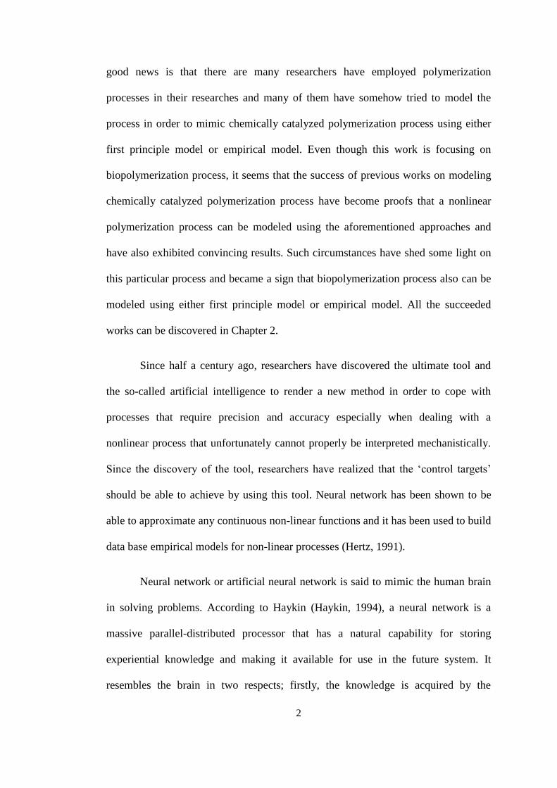
In other words, ANN is a simplified version of biological neuron. Biological-
artificial neuron analogy can be shown as in Table 2.1 below. Figure 2.1 gives a
pictorial representation of this biological-artificial terminology.
Table 2.1: Biological-Artificial Neuron Analogy (Statsoft Electronics
Statistical Textbook, 2010)
Biological Neurons Artificial Neural Networks
Soma Neuron
Dendrite Input
Axon Output
Synapse Weight
Page 39
15
(a)
(b)
Figure 2.1: (a) Biological Neuron; (b) Artificial Neural Network
Representation (Statsoft Electronics Statistical Textbook, 2010)
Therefore, neural network becomes one of the artificial intelligence
techniques. It is very similar to biological neurons in so many levels. Besides
similarities with biological neurons, neural network comprises of three common
layers:
Page 40
16
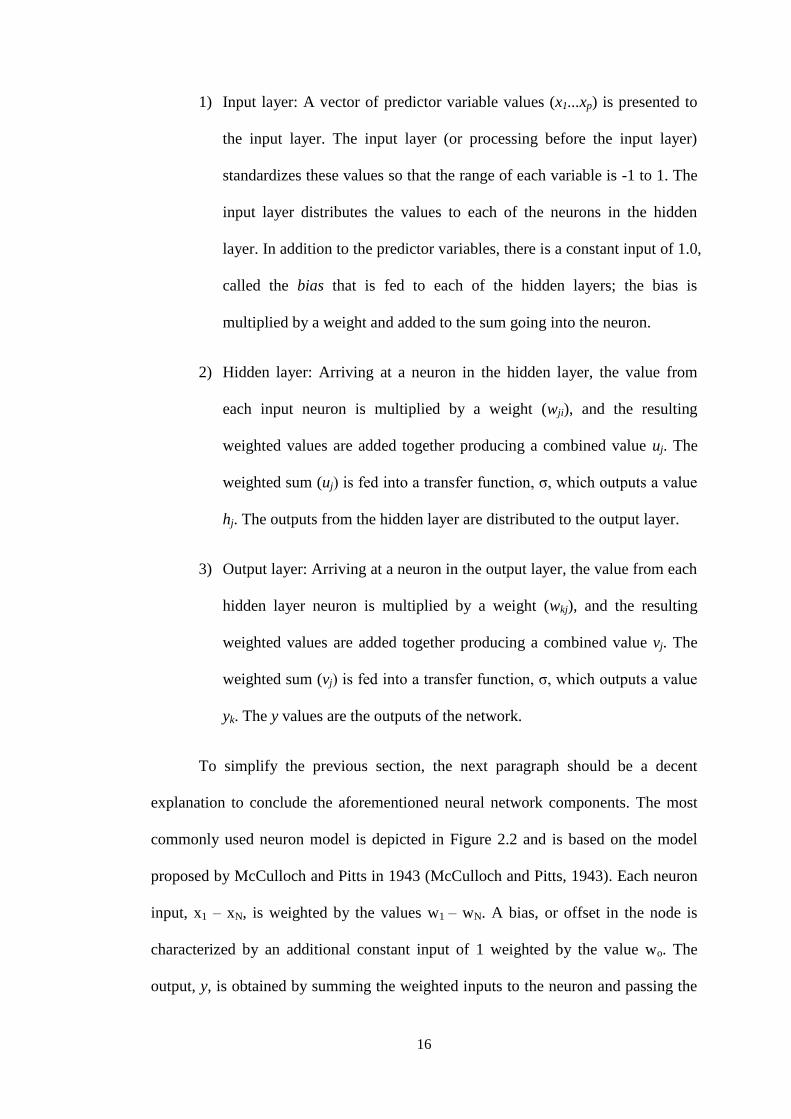
1) Input layer: A vector of predictor variable values (x1...xp) is presented to
the input layer. The input layer (or processing before the input layer)
standardizes these values so that the range of each variable is -1 to 1. The
input layer distributes the values to each of the neurons in the hidden
layer. In addition to the predictor variables, there is a constant input of 1.0,
called the bias that is fed to each of the hidden layers; the bias is
multiplied by a weight and added to the sum going into the neuron.
2) Hidden layer: Arriving at a neuron in the hidden layer, the value from
each input neuron is multiplied by a weight (wji), and the resulting
weighted values are added together producing a combined value uj. The
weighted sum (uj) is fed into a transfer function, σ, which outputs a value
hj. The outputs from the hidden layer are distributed to the output layer.
3) Output layer: Arriving at a neuron in the output layer, the value from each
hidden layer neuron is multiplied by a weight (wkj), and the resulting
weighted values are added together producing a combined value vj. The
weighted sum (vj) is fed into a transfer function, σ, which outputs a value
yk. The y values are the outputs of the network.
To simplify the previous section, the next paragraph should be a decent
explanation to conclude the aforementioned neural network components. The most
commonly used neuron model is depicted in Figure 2.2 and is based on the model
proposed by McCulloch and Pitts in 1943 (McCulloch and Pitts, 1943). Each neuron
input, x1 – xN, is weighted by the values w1 – wN. A bias, or offset in the node is
characterized by an additional constant input of 1 weighted by the value wo. The
output, y, is obtained by summing the weighted inputs to the neuron and passing the
Page 41
17
results through a nonlinear activation function, f ( ). Various types of nonlinearity are
possible and some of these are hard limiter, threshold logic, tanh and sigmoidal
functions. The general equation can be seen as the following:
𝑦 = 𝑓 𝑤𝑖𝑥𝑖 + 𝑤𝑜
𝑁
𝑖=1
(2.1)
Figure 2.2: Biological Neuron Elements-Artificial Neural Network Elements
(Warwick, 1995)
Among the numerous attributes of neural networks that have been found in many
application areas are (Warwick, 1995):
1) Inherent parallelism in the network architecture due to the repeated use of
simple neuron processing elements. This leads to the possibility of very fast
hardware implementations of neural networks.
f
W1
W2
WN
Wo
X1
X2
XN
Axons Synapses
Inputs Weights
Bias
Nonlinearit
y
Dendrites Body
1
y
Axon
Output
Page 42
18
2) Capability of learning information by example. The learning mechanism is
often achieved by appropriate adjustment of the weights in the synapses of
neural networks.
3) Ability to generalize to new inputs (i.e. trained ANN is capable of providing
„sensible‟ outputs when presented with input data that has not been used
before).
4) Robustness to noisy data that occurs in real world applications.
5) Fault tolerance. In general, ANN performance does not significantly
degenerate if some of the network connections become faulty.
The above attributes of neural networks indicate their potential in solving many
problems. Hence, the considerable interest in neural networks that has occurred in
recent years is not only due to significant advances in computer processing power
that has enabled their implementation but because of the diverse possibility of
application areas. Many different types of neural network architectures are available
for modeling and also control purposes. The next section is over viewing on types of
neural networks.
2.1 Types Of Neural Network
Nowadays, many types of neural network architectures are available to be
implemented. Amongst them are Hopfield, Kohonen, Radial Basis Function and the
most common network is Feedforward artificial neural network (FANN). A Hopfield
network is a type of recurrent network which was invented by John Hopfield. The
Hopfield network comprises of two layers, an input layer and a Hopfield layer. Each
Page 43
19
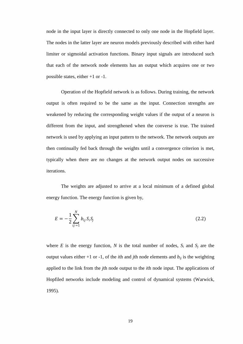
node in the input layer is directly connected to only one node in the Hopfield layer.
The nodes in the latter layer are neuron models previously described with either hard
limiter or sigmoidal activation functions. Binary input signals are introduced such
that each of the network node elements has an output which acquires one or two
possible states, either +1 or -1.
Operation of the Hopfield network is as follows. During training, the network
output is often required to be the same as the input. Connection strengths are
weakened by reducing the corresponding weight values if the output of a neuron is
different from the input, and strengthened when the converse is true. The trained
network is used by applying an input pattern to the network. The network outputs are
then continually fed back through the weights until a convergence criterion is met,
typically when there are no changes at the network output nodes on successive
iterations.
The weights are adjusted to arrive at a local minimum of a defined global
energy function. The energy function is given by,
𝐸 = −1
2 𝑏𝑖𝑗𝑆𝑖𝑆𝑗
𝑁
𝑖𝑗=1
(2.2)
where E is the energy function, N is the total number of nodes, Si and Sj are the
output values either +1 or -1, of the ith and jth node elements and bij is the weighting
applied to the link from the jth node output to the ith node input. The applications of
Hopfiled networks include modeling and control of dynamical systems (Warwick,
1995).
Page 44
20
A Kohonen network is constructed of a fully interconnected array of neurons
that is the output of each neuron is an input to all neurons including itself and each
neuron receives the input pattern. The distinguishing feature of this network from
other networks is that no output data is required for training. It has been developed
by Teuvo Kohonen (1989, 1995). There are two sets of weights; 1) an adaptable set,
to compute the weighted sum of the external inputs, 2) fixed set between neurons that
controls neuron interactions in the network.
Figure 2.3: A Simplified Kohonen Network (Heaton Research, 2010)
Kohonen network defines a mapping from the input data space spanned by
x1..xn onto a one- or two-dimensional array of nodes. The mapping is performed in a
way that the topological relationships in the n-dimensional input space are
maintained when mapped to the Kohonen network. In addition, the local density of
data is also reflected by the map: areas of the input data space which are represented
by more data are mapped to a larger area of the network.
Each node of the map is defined by a vector wij whose elements are adjusted
during the training. The basic training algorithm is quite simple; 1) select an object
Page 45
21
from the training set, 2) find the node which is closest to the selected data (i.e. the
distance between wij and the training data is a minimum), 3) adjust the weight
vectors of the closest node and the nodes around it in a way that the wij move towards
the training data, 4) repeat from step 1 for a fixed number of repetitions. The amount
of adjustment in step 3 as well as the range of the neighborhood decreases during the
training. This ensures that there are coarse adjustments in the first phase of the
training, while fine tuning occurs during the end of the training.
This form of training has the effect of organizing the „map‟ of the output
nodes such that different areas of the map will respond to different input patterns.
Hence, the Kohonen network has self-organizing properties and is capable of
recognition. Application examples of the Kohonen network include recognition of
images and speech signals (SDL Component Suite, 2008). The next section focuses
on the most common type of network which is the feedforward artificial neural
network (FANN) that has also been implemented in this work.
2.2 Feedforward Artificial Neural Network (FANN)
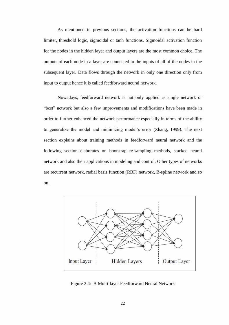
The most popular neural network architecture is the feedforward neural
network. Figure 2.4 shows typical feedforward neural network architecture. The
previous sections have circumstantially touched on this topic. The network consists
of an input layer, a number of hidden layers and an output layer. The output and
hidden layer are made up of a number of nodes. However, the input layer is
essentially a direct link to the inputs of the first hidden layer (Gomm et al., 1993). An
individual node in the network can be described by Equation 2.1.
Page 46
22
As mentioned in previous sections, the activation functions can be hard
limiter, threshold logic, sigmoidal or tanh functions. Sigmoidal activation function
for the nodes in the hidden layer and output layers are the most common choice. The
outputs of each node in a layer are connected to the inputs of all of the nodes in the
subsequent layer. Data flows through the network in only one direction only from
input to output hence it is called feedforward neural network.
Nowadays, feedforward network is not only applied as single network or
“best” network but also a few improvements and modifications have been made in
order to further enhanced the network performance especially in terms of the ability
to generalize the model and minimizing model‟s error (Zhang, 1999). The next
section explains about training methods in feedforward neural network and the
following section elaborates on bootstrap re-sampling methods, stacked neural
network and also their applications in modeling and control. Other types of networks
are recurrent network, radial basis function (RBF) network, B-spline network and so
on.
Figure 2.4: A Multi-layer Feedforward Neural Network
Page 47
23
Neural networks have also gone through a revolution in their applications
when improvements to the neural network such as bootstrap re-sampling method and
multiple neural networks are introduced. The goal of introducing these improved
methods for neural network is mainly to tackle problems such as lack of
generalization capability and also phenomena called overfitting and underfitting.
These drawbacks are usually encountered within the neural networks. Despite of
their differences, these methods possess similar mathematical concept especially the
one that is used in training. Training is an important step in developing neural
network models. Model robustness is primarily related to the learning or training
methods and the amount and representativeness of the training data. In other
words,training is one of the methods that enable neural network to learn about the
dynamic of a process in order to be able to generalize the process.
2.2.1 Training Paradigms in Feedforward Artificial Neural Network
The goal of the neural network training/learning process is to find the set of
weight values that will cause the output from the neural network to match the actual
target values as closely as possible. There are several issues involved in designing
and training a feedforward neural network: 1) Selecting how many hidden layers to
use in the network, 2) Deciding how many neurons to use in each hidden layer, 3)
Finding a globally optimal solution that avoids local minima, 4) Converging to an
optimal solution in a reasonable period of time, 5) Validating the neural network to
test for over fitting.
Learning in neural network is achieved by adjusting the modifiable
connection weights between the units as shown in Figure 2.5. As shown in Figure 2.5,
a set of neural networks is trained by adjusting weights and number of hidden
Page 48
24
neurons in the system. The resulting output from the training process is compared
with the targeted output value. The process continues until the resulting output from
the system and the targeted output are matched. The moment both outputs are
synchronized, the neural networks are considered as well trained and the process
proceeds to the testing and validation steps.
Figure 2.5: Basic Neural Network Training Method
Learning in neural networks is a problem of finding a set of connection
weights which would enhance the ability of neural networks to store experiential
knowledge; hence the learned knowledge can be used to achieve the desired response
in the future. Up to now, there are various choices of learning algorithms available,
and they can be classified into three main classes; supervised learning, reinforcement
or graded learning and unsupervised learning. A supervised learning algorithm
adjusts the strength or weights of the inter-neuron connections according to the
difference between the desired and actual network outputs corresponding to a given
input. Thus, supervised learning requires a “teacher” or “supervisor” to provide
desired or target output signals.
Page 49
25
Backpropagation (BP) algorithm is one of the notable supervised learning
algorithms. This approach basically refers to an external agent like computer
program that totally monitors the input and output vector pairs and adjusts the
weights in such a way that matches each network output with its target value. Other
commonly used supervised learning algorithms are Levenberg-Marquardt and
gradient descent method. Reinforcement learning algorithm is also similar to the
supervised learning except that the desired output is not provided. It employs a critic
only to evaluate the goodness of the neural network output corresponding to a given
output. Genetic algorithm (GA) is an example of the reinforcement learning
algorithm.
Unsupervised learning on the contrary, uses only the input vector for network
training and the network regulates its own weights without the benefits of knowing
what particular output to assign for a given input. During training, only input patterns
are presented to the neural network which automatically adapts the weights of its
connections to cluster the input patterns into groups with similar features. Kohonen
Rule for training Kohonen network is one example of unsupervised learning and also
Carpenter-Grossberg Adaptive Resonance Theory (ART) algorithm.
2.2.2 Levenberg- Marquardt (LM) Training Paradigm
Levenberg-Marquardt is a virtual standard in nonlinear optimization which
significantly outperforms gradient descent and conjugate gradient methods. It is a
pseudo-second order method which means that it works with only function
evaluations and gradient information but it estimates the Hessian matrix using the
sum of outer products of the gradients (Roweis, 2005) . The technique that


![4. Process Modeling - · PDF file4. Data Analysis for Process Modeling ... References For Chapter 4: Process Modeling [4.7.] ... 4. Process Modeling 4.1.Introduction to Process Modeling](https://static.documents.pub/doc/80x56/5a792f037f8b9a07628d27df/4-process-modeling-data-analysis-for-process-modeling-references-for-chapter.jpg)


