Modeling of Cross Polarization Tracking Errors of...

Modeling of Cross Polarization Tracking Errors of Radome-Enclosed Monopulse Systems

Senglee Foo, Louie Aloisius and Satish Kashyap

Defence R&D Canada √ Ottawa TECHNICAL REPORT

DRDC Ottawa TR 2003-153 March 2003

Modeling of Cross Polarization Tracking Errors of Radome-Enclosed Monopulse Systems

Senglee Foo, Louie Aloisius, Satish Kashyap

Defence R&D Canada – Ottawa Technical Report DRDC Ottawa TR 2003-153 March 2003

© Her Majesty the Queen as represented by the Minister of National Defence, 2003

© Sa majesté la reine, représentée par le ministre de la Défense nationale, 2003

DRDC Ottawa TR 2003-153 i

Abstract

A cross-polarized signal transmitted by a jammer passes through a protective radome before reaching the aperture of a missile antenna. As a result, the actual co-polar and cross-polar tracking response of the monopulse system changes and varies with the relative antenna-pointing angle. This study describes a systematic EM procedure for the prediction of the co-polar and cross-polar radiation patterns of radome-enclosed antennas. Both the measured and predicted results show that the presence of a radome significantly affects the susceptibility of a monopulse tracking system to the cross-polar jamming. In fact, the effectiveness of the cross-polar jamming depends on various factors such as the incidence angle, polarization angle, the shape and material of the radome, and the type of the antenna. Results of this study show that the cross-polar jamming in general does not have 100% of coverage angles. It is effective only in certain incidence angles and when the polarization angle is less than 30 deg. For some incidence angles, cross-polar jamming is deemed to be ineffective.

Résumé

Un signal contrapolaire émis par un brouilleur traverse un radôme de protection avant d’atteindre l’ouverture d’une antenne de missile. La réponse de poursuite copolaire et contrapolaire réelle du système monopulse change alors et elle varie en fonction de l’angle relatif de pointage de l’antenne. La présente étude décrit une procédure EM systématique de prévision des diagrammes de rayonnement copolaire et contrapolaire d’antennes confinées dans un radôme. Tant les valeurs mesurées que les valeurs prévues montrent que la présence d’un radôme influe de façon significative sur la sensibilité d’un système de poursuite monopulse au brouillage contrapolaire. En fait, l’efficacité du brouillage contrapolaire dépend de divers facteurs, comme l’angle d’incidence, l’angle de polarisation, la forme et la composition du radôme, et le type d’antenne. Les résultats de l’étude montrent qu’en général le brouillage contrapolaire n’offre pas une couverture angulaire de 100 %. Il est efficace seulement à certains angles d’incidence et lorsque l’angle de polarisation est inférieur à 30 degrés. À certains angles d’incidence, on considère que le brouillage contrapolaire est efficace.

ii DRDC Ottawa TR 2003-153

Executive summary A dielectric radome can introduce considerable distortion in the EM field patterns of a missile radar antenna. The cross-polar component of the field can be used to distort the normal operation of the missile radar tracker. This report is concerned with the measurement and computation of cross-polar field components and the effectiveness of cross-polar jamming. A general radome analysis procedure, based on a hybrid of the method-of-moments (MOM) and the EM ray tracing, is implemented for the modeling of cross-polar jamming. The method allows modeling of radome-enclosed antenna problems of arbitrary shape and is numerically very efficient. Computations and measurements are done on a scale model of the ogive shaped radome. Simulations compare well with the measurements for the co-polar components. Predictions of the cross-polar components are inherently more challenging due to the relatively low level in comparison to the co-polar component. The proposed scheme is able to produce cross-polar results that are adequate for assessment of monopulse tracking errors in the presence of a cross-polar jamming signal. Results show that a missile radome distorts both the co-polar and cross-polar patterns significantly. A monopulse system is susceptible to the cross-polar jamming only if a null appears near the boresight of the cross-polar pattern. In the presence of a radome, this condition depends on various factors such as the incidence angle, polarization angle, the shape and material of the radome, and the type of antenna. As a result, the coverage angle of susceptibility of a monopulse system to cross-polar jamming signal is less than 100%. In fact, in some incidence angles, the jamming signal can have an adverse effect and can enhance the tracking performance of the monopulse tracking response. This investigation is based on the use of rectangular horns as the antennas for the monopulse system. Further investigation is required to determine if such effect also holds for a more commonly used reflector antenna monopulse system.

Foo, S., Louie, A., Kashyap, S. (2003). Modeling of cross polarization tracking errors of radome-enclosed monopulse systems. DRDC Ottawa TR 2003-153. Defence R&D Canada - Ottawa.

DRDC Ottawa TR 2003-153 iii

Sommaire Un radôme diélectrique peut déformer considérablement les diagrammes de champ EM d’une antenne radar de missile. La composante contrapolaire du champ peut être utilisée pour perturber le fonctionnement normal du circuit de poursuite radar de missile. Le rapport traite de la mesure et du calcul des composantes contrapolaires du champ et de l’efficacité du brouillage contrapolaire. Une procédure générale d’analyse de radôme, basée sur une combinaison de la méthode des moments (MOM) et de la technique de tracé des rayons EM, est mise en œuvre pour la modélisation du brouillage contrapolaire. Elle permet de modéliser les problèmes associés aux antennes confinées dans un radôme de forme arbitraire et elle est très efficace sur le plan numérique. Les calculs et les mesures sont effectués sur un modèle à l’échelle du radôme en forme d’ogive. Dans le cas des composantes copolaires, les valeurs obtenues dans les simulations correspondent de près aux valeurs mesurées. Les prévisions des composantes contrapolaires sont intrinsèquement plus complexes, car ces composantes sont relativement faibles par comparaison aux composantes copolaires. La méthode proposée permet d’obtenir des résultats concernant les composantes contrapolaires qui sont adéquats pour l’évaluation des erreurs de poursuite monopulse en présence d’un signal de brouillage contrapolaire. Les résultats montrent qu’un radôme de missile perturbe de façon appréciable les diagrammes de rayonnement copolaire et contrapolaire. Un système monopulse est sensible au brouillage contrapolaire seulement si une extinction est observée à proximité de l’axe de visée du diagramme de rayonnement contrapolaire. En présence d’un radôme, cette condition dépend de divers facteurs, comme l’angle d’incidence, l’angle de polarisation, la forme et la composition du radôme, et le type d’antenne. Par conséquent, un système monopulse n’est pas sensible au signal de brouillage contrapolaire sur une couverture angulaire de 100 %. En fait, à certains angles d’incidence, le signal de brouillage peut produire un effet contraire et peut accroître l’efficacité de poursuite de la réponse monopulse. Cette étude est basée sur l’utilisation de cornets rectangulaires comme antennes du système monopulse. Une étude plus approfondie est nécessaire pour déterminer si cet effet se produit également dans le cas d’un système monopulse à antenne à réflecteur d’usage plus courant.

Foo, S., Louie, A., Kashyap, S. (2003). Modeling of cross polarization tracking errors of radome-enclosed monopulse systems. DRDC Ottawa TR 2003-153. R & D pour la défense Canada - Ottawa.

iv DRDC Ottawa TR 2003-153

Table of contents

Abstract........................................................................................................................................ i

Résumé ........................................................................................................................................ i

Executive summary .................................................................................................................... ii

Sommaire................................................................................................................................... iii

Table of contents ....................................................................................................................... iv

List of figures ............................................................................................................................ vi

List of tables .............................................................................................................................. ix

1. Introduction ............................................................................................................................ 1

2. Computational electromagnetics of pyramidal horns ............................................................. 2 2.1 Geometry of the pyramidal horn antenna ................................................................ 2 2.2 The first JUNCTION model of the PHA................................................................. 3 2.3 Mismatch analysis ................................................................................................... 5 2.4 The second JUNCTION models of the PHA........................................................... 6 2.5 The NEC model of the PHA.................................................................................... 8

3. Radome modeling................................................................................................................. 10 3.1 Objective................................................................................................................ 10 3.2 Definitions of polarizations ................................................................................... 10 3.3 Analysis methodology ........................................................................................... 10

3.3.1 Analysis procedures .................................................................... 10

3.3.2 Numerical aperture integration.................................................... 11

3.3.3 Dielectric flat-plate model........................................................... 13 3.4 Radome geometry and near-field generation......................................................... 15 3.5 Measurements........................................................................................................ 25 3.6 Simulations and result comparisons ...................................................................... 25

DRDC Ottawa TR 2003-153 v

4. Monopulse analysis .............................................................................................................. 35 4.1 Introduction ........................................................................................................... 35 4.2 Monopulse analysis using measured data.............................................................. 37 4.3 Comparing simulations with measured results ...................................................... 46 4.4 Tracking errors ...................................................................................................... 55

5. Discussion............................................................................................................................. 66

6. Conclusions .......................................................................................................................... 67

References ................................................................................................................................ 68

List of abbreviations/acronyms ................................................................................................ 71

Annex A: Measured radiation patterns .......................................................................................B

Annex B: Comparisons of squint-beam patterns ........................................................................E

vi DRDC Ottawa TR 2003-153

List of figures

Figure 1. The pyramidal horn antenna model 3160-07 ............................................................. 2

Figure 2. The triangular patch JUNCTION model PHA_J1 ..................................................... 3

Figure 3. JUNCTION-computed results versus DFL-measured data........................................ 4

Figure 4. The triangular patch JUNCTION model PHA_J2 ...................................................... 6

Figure 5. JUNCTION-computed results versus DFL-measured data......................................... 7

Figure 6. The wire-grid NEC model PHA_N............................................................................ 8

Figure 7. NEC-computed results versus DFL-measured data ................................................... 9

Figure 8. Propagation vectors in a dielectric flat plate ............................................................. 14

Figure 9. Radome enclosed PHA ............................................................................................. 15

Figure 10. Radome and PHA geometry................................................................................... 16

Figure 11. Coordinate system when antenna pointing angle is 0 deg...................................... 18

Figure 12. Coordinate system when antenna pointing angle is 30 deg..................................... 19

Figure 13. Coordinate system when antenna pointing angle is 45 deg..................................... 20

Figure 14. Ogive radome discretization and normal vectors ................................................... 21

Figure 15. Ex near-field distribution ....................................................................................... 22

Figure 16. Ey near-field distribution ....................................................................................... 22

Figure 17. Ez near-field distribution......................................................................................... 23

Figure 18. Hx near-field distribution........................................................................................ 23

Figure 19. Hy near-field distribution........................................................................................ 24

Figure 20. Hz near-field distribution ........................................................................................ 24

Figure 21. Radome test configuration at DFL.......................................................................... 25

Figure 22. Simulated and measured co-polar patterns of X-band PHA ................................... 26

Figure 23. Co-polar patterns of radome/PHA with antenna pointing angle=0 deg .................. 27

DRDC Ottawa TR 2003-153 vii

Figure 24 Co-polar patterns of radome/PHA with antenna pointing angle=30 deg ................ 28

Figure 25. Co-polar patterns of radome/PHA with antenna pointing angle=45 deg ............... 29

Figure 26. Cross-polar patterns of X-band Horn ...................................................................... 31

Figure 27. Cross-polar patterns of radome/PHA with antenna pointing angle=0 deg.............. 32

Figure 28. Cross-polar patterns of radome/PHA with antenna pointing angle=30 deg........... 33

Figure 29. Cross-polar patterns of radome/PHA with antenna pointing angle=45 deg............ 34

Figure 30. Monopulse patterns and tracking errors with squint angle=5.0 deg........................ 36

Figure 31. E-plane Monopulse patterns of the X-band Horn ................................................... 38

Figure 32. H-plane Monopulse patterns of the X-band Horn ................................................... 39

Figure 33. E-plane Monopulse patterns of with antenna pointing angle=0 deg ....................... 40

Figure 34. H-plane Monopulse patterns with antenna pointing angle=0 deg........................... 41

Figure 35. E-plane Monopulse patterns with antenna pointing angle=30 deg ......................... 42

Figure 36. H-plane Monopulse patterns with antenna pointing angle=30 deg......................... 43

Figure 37. E-plane Monopulse patterns with antenna pointing angle=45 deg ......................... 44

Figure 38. H-plane Monopulse patterns with antenna pointing angle=45 deg......................... 45

Figure 39. Simulated E-plane Monopulse patterns of the X-band Horn ................................. 47

Figure 40. Simulated H-plane Monopulse patterns of the X-band Horn................................. 48

Figure 41. Simulated E-plane patterns antenna pointing angle=0 deg ..................................... 49

Figure 42. Simulated H-plane patterns with antenna pointing angle=0 deg............................. 50

Figure 43. Simulated E-plane patterns with antenna pointing angle=30 deg ........................... 51

Figure 44. Simulated H-plane patterns with antenna pointing angle=30 deg........................... 52

Figure 45. Simulated E-plane patterns with antenna pointing angle=45 deg ........................... 53

Figure 46. Simulated H-plane patterns with antenna pointing angle=45 deg........................... 54

Figure 47. Tracking errors without radome.............................................................................. 57

Figure 48. Tracking errors with antenna pointing angle=0 deg............................................... 58

viii DRDC Ottawa TR 2003-153

Figure 49. Tracking errors with antenna pointing angle=30 deg............................................. 59

Figure 50. Tracking errors with antenna pointing angle=45 deg............................................. 60

Figure 51. Tracking errors with polarization angle=0 deg ...................................................... 61

Figure 52. Tracking errors with polarization angle=10 deg .................................................... 62






Figure 58. Tracking errors versus polarization angles............................................................. 65

DRDC Ottawa TR 2003-153 ix

List of tables

Table 1. Parameter comparison: Junction versus measured results........................................... 5

Table 2. Radome/PHA geometry parameters .......................................................................... 17

Table 3. Cross-polar jamming effectiveness: measurements versus simulations ..................... 46

Table 4. Tracking Errors........................................................................................................... 55

x DRDC Ottawa TR 2003-153

This page intentionally left blank.

DRDC Ottawa TR 2003-153

1

1. Introduction

Defence Research & Development Canada (DRDC) has been involved in research related to the cross-polarization jamming in the past [16]. This report supplements the previous works by the EM modeling of the protective radome enclosing the tracking antenna. The primary objective is to enable accurate modeling of radome-enclosed antenna and to determine a systematic method for quantitative assessment of the radome effect on monopulse tracking response in the presence of a cross-polarized jamming signal.

A cross-polarized signal transmitted from a jammer passes through a radome before arriving at the antenna elements of a monopulse tracking system. At X-band frequency, the distortion in the cross-polar signal is significant and varies depending on the geometry and material properties of the radome, and incidence angle of the jamming signal. Unfortunately, modeling of the radome involves inhomogeneous materials and complex problem geometry that has a typical dimension in the orders of many wavelengths. These types of problems, in general, cannot be analysed using commercially available EM packages that utilize a full-wave approach such as the method of moments (MOM), finite element method (FEM), finite difference time domain method (FDTD). Radome problems are almost exclusively analysed by using high-frequency approximation methods such as ray tracing [1-13]. A conventional ray-tracing method works well for prediction of co-polar radiation patterns of a relatively large radome. However, the conventional ray tracing, per se, is not suitable for prediction of low-level cross-polar patterns, which are typically more than -30dB below the co-polar signals. This is especially difficult when the problem involves a medium-sized, highly shaped radome such as an ogive tangent radome.

Paris [1] proposes a procedure that uses the near-field values of a radiating antenna and a flat plate model for the dielectric radome to predict the radiation pattern of a radome-enclosed rectangular horn. This technique models the exact geometry of the antenna including its surrounding near-field and therefore gives a better prediction for the cross-polar pattern. A similar procedure based on the method of moments for the near-field analysis is adopted here. The method generates the near-field data on the inside surface of the radome using the method of moments. The field on the outside of the radome is then calculated using the dielectric flat-plate method. The co-polar and cross-polar patterns of the antenna system are then calculated using aperture integration.

Monopulse patterns are simulated using the measured antenna/radome patterns. Results show that the effectiveness of the cross-polar jamming depends largely on the antenna type, properties of the radome, look angle and the signal strength of the jamming signal. The coverage angle (% of total angular space) of susceptibility of a monopulse system to cross-polar jamming is, in general, less than 100%.

2 DRDC Ottawa TR 2003-153

2. Computational electromagnetics of pyramidal horns

2.1 Geometry of the pyramidal horn antenna A standard gain pyramidal horn antenna (PHA) manufactured by EMCO (model 3160-07) is used as the feed antenna for this study. The PHA flares in both E-plane and H-plane and is attached to a short waveguide (WR90). Fig.1 shows the physical dimensions of the PHA.

B = 5.80 cm

a = 2.286 cmb = 1.016 cm

d = 1.143 cmWR90

voltage source(from within)

E-plane

H-plane

Figure 1. The pyramidal horn antenna model 3160-07

All dimensions given in Fig.1 are the interior dimensions, which are used as the actual parameters in the numerical model. The rectangular waveguide WR90 has the interior dimensions of a = 2.286 cm and b = 1.016 cm. This gives a lower cut-off frequency at 6.557 GHz and cut-off wavelength of 4.572 cm for the TE10 mode. The excitation is a voltage source applied to a wire segment placed at 1.143 cm from the back end of the waveguide. The operating frequency for this study is 9.2 GHz.

DRDC Ottawa TR 2003-153 3

2.2 The first JUNCTION model of the PHA In the first attempt, a method-of-moments code, namely, JUNCTION [23] is used to model the problem geometry. This MOM code model metallic surfaces as a finite union of triangular patches. The first model called PHA_J1 consists of 2804 triangular patches.

z

y

x

2

N

Figure 2. The triangular patch JUNCTION model PHA_J1

Fig. 2 shows the PHA in its standard orientation, i.e., antenna pointing angle=0 deg. In this position, the centre axis of the horn aligns with the x-axis; therefore, the maximum gain is in the +x direction (i.e. 0=φ deg and 90=θ deg). As a result, the H-plane is at θ=90 deg and

the E-plane is at Ф=0 deg. The voltage source excitation is provided by a single thin wire

segment, 0.5 mm radius and 5.1 mm length, attached to the topside of the waveguide (see Fig. 1). The edge lengths of the triangular plates are maintained to within 5 mm. By the “ 5/λ -rule ”, the maximum frequency of this model is about 12 GHz. The PHA_J1 model is built such that all edges are approximately of the same length, approximately 5mm, which is less than 5.6/λ at 9.2 GHz. Fig.3 compares the computed gain patterns with the measured results on the H- and E-planes, respectively. The measured gain is 16.4 dB. The computed gain is slightly lower and a scale constant is included to match the patterns. The same scale factor is applied to the co-polarized gain and the cross-polarized gain.


(A) H-plane pattern

- 1 0 0 - 5 0 0 5 0 1 0 0- 6 0

- 4 0

- 2 0

0

2 0

A zim uth N (E)

*E2*

*EN*

com putedmeasured

(B) E-plane pattern

0 60 9 0 1 50 1 8 0- 6 0

- 4 0

- 2 0

0

2 0

Elevation 2 (E)

*E2*

*EN*

1 2 03 0

computedmeasured

Figure 3. JUNCTION-computed results versus DFL-measured data


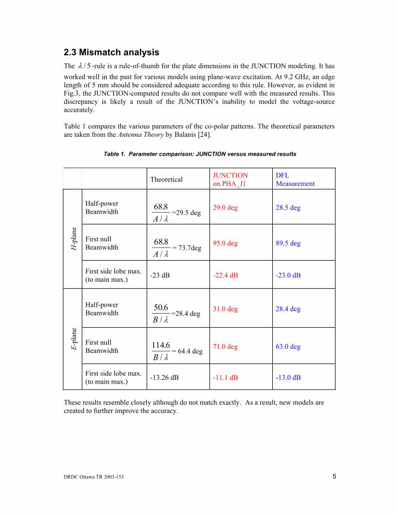
2.3 Mismatch analysis The 5/λ -rule is a rule-of-thumb for the plate dimensions in the JUNCTION modeling. It has worked well in the past for various models using plane-wave excitation. At 9.2 GHz, an edge length of 5 mm should be considered adequate according to this rule. However, as evident in Fig.3, the JUNCTION-computed results do not compare well with the measured results. This discrepancy is likely a result of the JUNCTION’s inability to model the voltage-source accurately. Table 1 compares the various parameters of the co-polar patterns. The theoretical parameters are taken from the Antenna Theory by Balanis [24].

Table 1. Parameter comparison: JUNCTION versus measured results

Theoretical JUNCTION on PHA_J1

DFL Measurement

Half-power Beamwidth 68 8.

/A λ=29.5 deg

29.0 deg 28.5 deg

First null Beamwidth

68 8./A λ

= 73.7deg 95.0 deg 89.5 deg

H-p

lane

First side lobe max. (to main max.) -23 dB -22.4 dB -23.0 dB

Half-power Beamwidth

50 6./B λ

=28.4 deg 31.0 deg 28.4 deg

First null Beamwidth

114 6./B λ

= 64.4 deg 71.0 deg 63.0 deg E-

plan

e

First side lobe max. (to main max.) -13.26 dB -11.1 dB -13.0 dB

These results resemble closely although do not match exactly. As a result, new models are created to further improve the accuracy.


2.4 The second JUNCTION models of the PHA Fig.4 shows the second model PHA_J2, which has the same dimensions and orientation as PHA_J1. However, the edge lengths of the triangular plates are now maintained to within 3.25 mm, which is about one-tenth the wavelength at 9.2 GHz. The model consists of 5334 triangular patches.

z

y

x

2

N

Figure 4. The triangular patch JUNCTION model PHA_J2

This second model has over 8000 unknowns in the matrix equation, which is at the limit of the available computing resource. As shown in Fig. 5, this model does not provide significantly better results as compared with the previous model. This implies that the discretization of the model is not likely the primary source of the discrepancy.


(A) H-plane pattern

- 1 0 0 - 5 0 0 5 0 1 0 0- 6 0

- 4 0

- 2 0

0

2 0

*E2*

*EN*

Azim uth N (E)

computedmeasured

(B) E-plane pattern

0 6 0 9 0 1 5 0 1 8 0- 6 0

- 4 0

- 2 0

0

2 0

Elevation 2 (E)

*E2*

*EN*

1 2 03 0

computedmeasured

Figure 5. JUNCTION-computed results versus DFL-measured data


2.5 The NEC model of the PHA Fig.6 shows the third model of the feed antenna, PHA_N. This model is generated using a thin-wire method-of-moments code, namely, NEC [25]. This model is made of wire-grid and has the same discretization as PHA_J2, i.e. with wire segments less than 3.25 mm and has just over 5430 wires.

z

y

x

Figure 6. The wire-grid NEC model PHA_N

The wire-radius criterion for NEC is such that if parallel wire segments are at a distance s apart, then they should have a radius r so that sr =π2 , i.e., the resulting rectangular surfaces of flattened wire segments along the length should just cover up the space between the grids. For wire segments on the perimeter of an aperture, the wire radii are halved, i.e., 2/2 sr =π . This is because only one side of the open grid need to be covered. In the NEC model PHA_N, the average wire segment length (hence grid separation s) is 3.25 mm. Thus, the proper wire radius is 0.6 mm for interior wires and 0.3 mm for boundary wires. As shown in Fig. 7, the NEC-computed results compare well with the DFL-measured data. A scale constant is incorporated to match the peak value between the computed and measured data. Note that all the computed results are symmetrical with respect to the centre axis.


(A) H-plane pattern

- 1 0 0 - 5 0 0 5 0 1 0 0- 6 0

- 4 0

- 2 0

0

2 0

*E 2*

*EN*

A zim uth N (E)

com putedmeasured

(B) E-plane pattern

0 6 0 9 0 1 5 0 1 8 0- 6 0

- 4 0

- 2 0

0

2 0

Elevation 2 (E )

*E 2*

*E N*

1 2 03 0

com putedmeasu red

Figure 7. NEC-computed results versus DFL-measured data


3. Radome modeling 3.1 Objective The objective here is to formulate an EM modeling algorithm that enables accurate modeling of the cross-polar component produced by an antenna enclosed in a protective radome. Due to the complexity and size of the radome problem, a full-wave technique is in general not feasible. The proposed technique is based on a hybrid of the method-of-moments (MOM) and a high-frequency approximation method. 3.2 Definitions of polarizations In general, an amplitude vector of an EM plane wave can be expressed in terms of two linear, orthogonal polarization vectors:

RU = Reference polarization, or co-polar, and

XU = Cross polarization, or cross-polar. Several definitions exist for the computation and measurement of these two vectors. This report assumes the Ludwig’s third definition [15]. Note that the antenna to be modelled is a pyramidal horn with its boresight pointed in the x-axis and with the E-field excitation in the z direction. This results in a θ -oriented linear polarization (co-polar component) in the two principal planes of the main beam. The cross-polar component is the φ component along the E- and H-planes. 3.3 Analysis methodology A number of methods have been developed for prediction of radome effects in the past. These methods are based on the high frequency, geometrical optics approximation. The ray-tracing methods are less rigorous but have the advantage of a fast solution and is less demanding on computer resources. However, a conventional ray-tracing method, per se, does not allow exact modeling of the antenna characteristic and therefore is not suitable for cross-polar analysis. Aperture integration technique offers a more rigorous approach and is more accurate than a ray-tracing method. The proposed method is based on a hybrid of method of moments (MOM), aperture integration (AI) and ray tracing. 3.3.1 Analysis procedures A variation of this approach was first proposed by Paris[1] for prediction of antenna pattern of a rectangular horn antenna enclosed in a tangent ogive radome. Similar techniques were also used by Wu and Reduce[2] and Huddleston, Bassett and Newton [3][11][12]. This report presents a generalized extension of the method by coupling the aperture integration with the method of moments. This method models the full electrical characteristics of the antenna and allows modeling of arbitrary shaped, multiplayer dielectric radome. Effectively it models the full-wave EM propagation effects, except for the multiple-reflections between the radome and the antenna, which is relatively small for a large radome.


The procedure is similar to the one described by Paris [1] and can be summarized in four general stages:

1.Geometric Modeling of radome surface The inner surface of the radome is modeled by a number of triangular elements. Locations for the calculation of EM field points are specified and surface normal vector of the elements are computed. Dimension of the elements are constrained to a maximum of 0.2λ for first order field interpolation.

2.Near-field calculation The exact geometrical and electrical characteristics of the antenna are modeled using the method of moments. Complex EM near-field values are computed for all field points under the free-space condition, i.e., assuming the dielectric radome is absent.

3.Transmission coefficient insertion The propagation direction at each field point is calculated using the Poynting vector ( )∗× HE . Field quantities are decomposed into two orthogonal components with respect to the incidence plane. Transmission coefficients of the two components are calculated using local plane model. Total tangential field and the field locations on the outer surface are calculated.

4.Numerical aperture integration Integrate the EM field on the outer surface to form the far-field patterns.

3.3.2 Numerical aperture integration The free-space electric and magnetic fields over the entire inner surface of the radome are evaluated numerically using the method of moments. From these results, the equivalent current densities can be determined from the electric and magnetic vector potentials A and F. The outer surface So is sub-divided into N smaller areas where the vector potentials can be integrated numerically in terms of the local E and H values. By using local plane wave approximation at each sub-region, these quantities can be expressed in terms of the field quantities on the inner surface Ei, Hi, the transmission coefficients Γi, and the field interpolation function αi(x,y,z):

r

eArj

π

β

4

−

= ×n ∫∫ ′′⋅

So

rrjSo SdeH ˆβ

re rj

π

β

4

−

= ×n ∑=

N

iiQ

1

ˆ

r

eFrj

π

β

4

−

−= ×n ∫∫ ′′⋅

So

rrjSo SdeE ˆβ

re rj

π

β

4

−

−= ×n ∑=

N

iiP

1

ˆ

where ∫∫ ′= ′⋅

Si

rrjioi SdeHQ ˆˆ β = [ ][ ][ ] SdezyxaH rrj

iSi

iii ′⋅Γ ′⋅∫∫ ˆ),,(ˆ βα

∫∫ ′= ′⋅

Si

rrjioi SdeEP ˆˆ β = [ ][ ][ ] SdezyxaE rrj

iSi

iii ′⋅Γ ′⋅∫∫ ˆ),,(ˆ βα


Here iS indicates the surface area of dielectric plate i and αi(x,y,z) is field interpolation function. For simplicity, the first–order point-matching is used for the interpolation function, i.e., )(),,( oi rrzyx −= δα . As a result, the two integral equations are simplified to the following algebraic expressions: [ ][ ][ ] orrj

iiiii eAaHQ ⋅⋅Γ= ˆˆˆ β

[ ][ ][ ] orrjiiiii eAaEP ⋅⋅Γ= ˆˆˆ β

where Ai is the local surface area of sub-region i. This method works well for local surface area iS with maximum linear dimensions less than 0.2λ . For larger surface area, a higher order interpolation will be required. The local field components [ ]iH and [ ]iE , the dyadic transmission coefficients [ ]iΓ , and the unit vector matrix, [ ]ia , are defined at the inner surface of each dielectric plate as follows:

[ ]

ΓΓ

=Γ⊥

//00

i

ii , [ ]

=

⊥

//i

ii E

EE , [ ]

=

⊥

//i

ii H

HH , [ ]

=

⊥

//ˆˆ

ˆi

ii a

aa

The propagation factor expressed in terms of the observation angle at ( φθ , ) and the source coordinate at ),,( zyxr ′′′=′ is

( )θφθφθλπβ cossinsincossin2ˆ zyxrro

′+′+′=′⋅

The definitions and relationship of the unit vectors can be expressed as follows: iii kna ˆˆˆ ×=⊥

iii kaa ˆˆˆ // ×= ⊥

iii naa ˆˆˆ ×= ⊥ξ

ik =( )( )∗

∗

×

×

ii

ii

HEHE

ReRe

The unit vector ξ

ia is defined so that only the tangential components of the parallel field on the outer surface are retained, i.e., ( ) ( )ξξ

iiiiiiiii aEaaEaEEE ˆˆˆˆ//tan ⋅+⋅=+= ⊥⊥⊥

( ) ( )⊥⊥⊥ ⋅+⋅=+= iiiiiiiii aHaaHaHHH ˆˆˆˆ//tan ξξ The normalized far-field pattern can be obtained in terms of the tangential vector potentials as follows: tantan),( FA EEE +=φθ = rFjAj ˆˆˆ ×−− ωεηωµ = φηθη φθθφ

ˆ)(ˆ)( AFAF −++−


3.3.3 Dielectric flat-plate model Effects of the dielectric radome are included in the formulation by using the cascaded ABCD transmission matrix of a multi-layer dielectric plate [1][24]. This method includes the amplitude attenuation and insertion phase delay (IPD) of the radome and multiple reflections within the dielectric materials. Effect on polarization of the field components is also accurately modeled by resolving the field components into two orthogonal TE and TM field vectors at each local dielectric interface. A general formulation for the reflection [ ]//,ΓΓ⊥ and transmission [ ]//,TT⊥ coefficients of this configuration is as follows:

ΓΓ⊥⊥

////TT

=

⊥

⊥

⊥

⊥

i

r

i

t

i

r

i

t

EE

EE

EE

EE

//

//

//

//

=

0

0

0

0

0

0

1

1

CD

C

AB

A

where,

jA = 2

ieψ [ ])1()1( 1111 ++++ −++ jjjj YBYA , AN+1 = 1.0;

jB = 2

ie ψ−

[ ])1()1( 1111 ++++ ++− jjjj YBYA , BN+1 = 0.0;

jC = 2

ieψ [ ])1()1( 1111 ++++ −++ jjjj ZDZC , CN+1 = 1.0;

jD = 2

ie ψ−

[ ])1()1( 1111 ++++ ++− jjjj ZDZC , DN+1 = 0.0;

1+jY = j

j

θθ

coscos 1+

)tan1()tan1( 11

jj

jj

jj

δεδε

−

− ++

1+jZ = j

j

θθ

coscos 1+

)tan1()tan1(

11 ++ −

−

jj

jj

jj

δεδε

jγ = )( jjj jj ωεσωµ +± ≅ joλπ2

rjrjεµ , if 1tan <<δ

The refraction angle jθ can be determined by imposing the Snell’s law of reflection on the

dielectric interface, which leads to an explicit expression for low loss ( )1.0(tan <<jδ materials,

jjj

rjrjj θ

εµεµ

θ 2

111 sin1cos

−≅

+++


Note that the parameter jψ represents the phase angle, or the total electrical length traveled

inside medium j. This quantity has been cited [1] as jjjj d θγψ cos= , where dj is the

thickness of dielectric layer j, jγ is the propagation constant of medium j and the jθ is the refraction angle in layer j. This expression gives a phase angle that has a reverse relation versus the incidence angle. This behavior is inconsistent with the physical evidence that the electrical path length increases as the incidence angle increases. A more consistent expression for the phase angle can be derived with aid of Fig.8. Given a refraction angle jθ in medium j, the wave traveling direction in the medium j is given by, jjj yzk θθ sinˆcosˆˆ −⋅= and the position vector for the wave traveling in the general yz plane can be expressed as: zzyyr ⋅+⋅= ˆˆˆ The total distance of the wave traveled from one interface to the other can be found by taking a scalar product of the two vectors, i.e., jjj yzrk θθ sincosˆˆ −=⋅

Substituting jzy θtan−= into the above equation result in j

jzrkθcos

ˆˆ =⋅ . Therefore, the

phase angle at the second interface z = dj is:

jψ = rk jj ˆˆ ⋅γ = j

jjdθγ

cos

Figure 8. Propagation vectors in a dielectric flat plate

jd

jθ

y

z

k

iE//

v

iE⊥

v

rE//

r

rE⊥

v

tE//

v

tE⊥

v

),( zy


3.4 Radome geometry and near-field generation The thin-wire method-of-moments code, NEC, generates the near-field data on the inside surface of the radome. For this study, the radome takes typical tangent ogive geometry. A scaled model of the radome has been designed and built by the Communication Research Center (CRC). The radome is cast using high-purity ceramic with a dielectric constant of 11 and loss tangent of 0.03 at 10.0 GHz. The inside diameter of the radome is 20 cm at the base. The overall length of the radome measured from the base to the tip (inside) is 30 cm. The thickness of the radome wall is 1.0 cm. Fig. 9 shows an isometric view of the radome including the feed horn antenna.

x

y

z

0

Figure 9. Radome enclosed PHA

Revolving a longitudinal section about the x-axis forms the tangent ogive. The transverse sections (in the yz-plane) through this radome shape are circular. Fig. 9 and the following geometric parameters define the tangent ogive: 222)( RxEy =++ , Lx ≤≤0 , 2/0 Dy ≤≤ (1) Fig. 10 shows the parameters R, E, L and D and gives the reference coordinates system of the radome/antenna. It is a circular arc centred at C, spanning a sector angle of R.


RR

x

x

y

y

z

ztop view

side view

L

D

D

E

q

C

R

Figure 10. Radome and PHA geometry


For the three-dimensional case, y in (1) is replaced by 2/122 )( zy + The dimensions of the tangent ogive are more commonly expressed in terms of the base diameter D and the length L, which define the fineness ratio

DLF =

where21

≥F . The radome has a hemispherical shape when 21

=F . As the value of the F

increases, the radome shape becomes more pointed. The followings are the governing parameters:

The antenna-pointing angle is defined as the relative angle between the electrical boresight of the PHA and the tip of the radome. Fig. 11 shows the coordinate system of the radome/PHA when the antenna pointing angle is 0 deg. In this case, the axis is aligned on the x-axis, with the wire feed in the +z direction. The opening of the horn extends a distance of q into the radome. Thus the origin of the coordinate system is at the centre of a transverse section at an axial distance of q inside the horn. Table 2 lists the geometrical parameters of the radome/antenna assembly.

Table 2. Radome/PHA geometry parameters

base diameter D 0.20 m

Length L 0.30 m

E 0.40 m

R 0.50 m

Sector angle R 36.87E

Insertion distance of horn into radome q 0.05 m

To change the antenna pointing angle, the PHA is rotated in the H-plane pivoting at point p = -1.27cm from the Z-axis. Figs. 12 and 13 show the antenna-pointing angle at 30 deg and 45 deg case, respectively.

E L DD

=−4

4

2 2

RL D

D=

+44

2 2

( )D R E= −2

( )L R E= −2 212


x

x

y

y

z

z

top view

side view

q

z

xy

front view

q

P

p

Figure 11. Coordinate system when antenna pointing angle is 0 deg


x

x

y

y

z

ztop view

side view

z

x y

front view

P30E



x

x

y

y

z

z

top view

side view

z

x y

front view

P

45E



The ogive radome is not part of the NEC wire-grid model. Instead, the NEC computes the E-field and H-field values at a set of near-field points located on the inside surface of the radome. Each of these near-field points is the centroid of a triangular patch. At each location, the (x,y,z) coordinates, the corresponding normal vector on the radome, and the area of the triangular patch are reported along with the three coordinate-axis components of the near E-field and H-field. The same 10/λ -rule also applies to the field point distribution on the radome. Fig. 14 shows the discretization of the radome surface including the normal vectors of each triangular plate. A total of 5100 near-field points (triangular plates) are used to approximate the radome surface.

Figure 14. Ogive radome discretization and normal vectors

Figs. 15-20 show the magnitude of the six field components on the radome, when the antenna pointing angle is 0 deg. The principal components are Ez and Hy, the other four components are relatively small in magnitude.


-0 .1

-0 .0 5

0

0 .0 5

0 .1

z

00 .0 5

0 .10 .1 5

0 .20 .2 5

0 .3

x-0 .1

-0 .0 50

0 .0 50 .1y X Y

Z

|E x |2 .7 52 .52 .2 521 .7 51 .51 .2 510 .7 50 .50 .2 50

Figure 15. Ex near-field distribution

-0.1

-0 .05

0

0.05

0.1

z

00.05

0.10.15

0.20.25

0.3

x-0.1

-0.050

0.050.1y X Y

Z

|Ex|2.752.52.2521.751.51.2510.750.50.250

Figure 16. Ey near-field distribution


-0 .1

-0 .05

0

0 .05

0 .1

z

00 .05

0 .10 .1 5

0 .20 .25

0 .3

x-0 .1

-0 .050

0 .050 .1y X Y

Z

|E z|6 .565 .554 .543 .532 .521 .510 .50

Figure 17. Ez near-field distribution

-0 .1

-0 .0 5

0

0 .0 5

0 .1

z

00 .0 5

0 .10 .1 5

0 .20 .2 5

0 .3

x-0 .1

-0 .0 50

0 .0 50 .1y X Y

Z

|H x |0 .0 0 40 .0 0 3 50 .0 0 30 .0 0 2 50 .0 0 20 .0 0 1 50 .0 0 10 .0 0 0 50

Figure 18. Hx near-field distribution


-0 .1

-0 .05

0

0 .05

0 .1

z

00 .05

0 .10 .1 5

0 .20 .25

0 .3

x-0 .1

-0 .050

0 .050 .1y X Y

Z

|H y|0 .017 50 .0150 .012 50 .010 .007 50 .0050 .002 50

Figure 19. Hy near-field distribution

-0 .1

-0 .05

0

0 .05

0 .1

z

00 .05

0 .10 .1 5

0 .20 .25

0 .3

x-0 .1

-0 .050

0 .050 .1y X Y

Z

|H z |0 .001 50 .001 250 .0010 .000 750 .000 50 .000 250

Figure 20. Hz near-field distribution


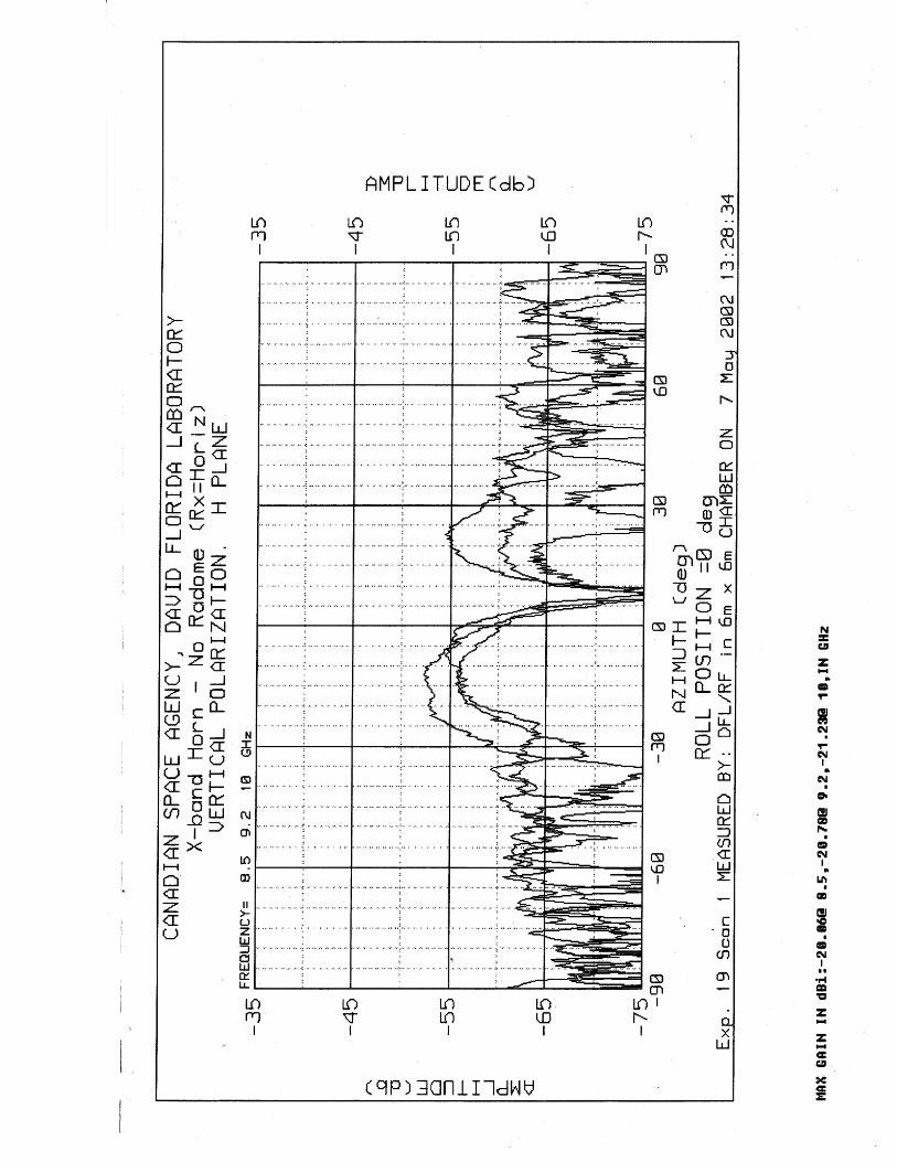
3.5 Measurements The far-field patterns of the radome/antenna in the two principal planes (E-plane and H-plane) were measured at the David Florida Lab (DFL) of the Canadian Space Agency (CSA). Fig. 21 shows the test configuration in the anechoic chamber. The co-polar and cross-polar patterns for various antenna-pointing angles were measured at three frequencies (8.5 GHz, 9.2 GHz, 10.0 GHz). These patterns are summarized in Annex A.

Figure 21. Radome test configuration at DFL

3.6 Simulations and result comparisons A numerical model of the radome/antenna was implemented based on the procedure described in the previous sections. The near-field values on the inside surface of the radome were generated using the method-of-moments (MOM) codes: JUNCTION and NEC. Fig. 22 compares the simulated and measured co-polar radiation patterns of the X-band feed horn without radome in the two principal planes.

Results are closely related among these methods. However, the near-field values obtained from the NEC code produce far-field patterns that compare better with the measurement. Figs. 23 to 25 show the comparisons between the simulations and measured co-polar patterns in the two principal planes of a radome enclosed PHA for antenna pointing angles at 0 deg, 30 deg and 45 deg. Except for the case where the antenna boresight is pointed directly at the tip of the radome, simulations in general agree well with the measured results within the main beam. In the case when the antenna pointing angle is 0 deg, the pattern does not match as well in some areas of the main beam due to the abrupt changes in the geometry at the tip of the ogive shape. Here the high-frequency approximation no longer holds well. The mismatch outside the main beam is expected, as the bottom surface of the radome is not included in the near-field model. For the purpose of this study, the area of concern is restricted to within the main beam of the patterns.


(A) E-plane Pattern

-10

-5

0

5

10

15

20

0 20 40 60 80 100 120 140 160 180

Scan angle [deg]

Gai

n [d

Bi]

NEC

DFL

Junction

E-plane @ 9.2 GHzNo Radome

(B) H-plane Patterns

-30

-25

-20

-15

-10

-5

0

5

10

15

20

0 20 40 60 80 100 120 140 160 180

Scan angle [deg]

Gai

n [d

Bi]

NEC

DFL

JUNCTION

H-plane @9.2 GHzNo Radome

Figure 22. Simulated and measured co-polar patterns of X-band PHA


(A) E-plane Co-polar Pattern

-15

-10

-5

0

5

10

15

0 20 40 60 80 100 120 140 160 180

Scan angle [deg]

Gai

n [d

B]

DFLNEC MOM

Ceramic Radome Er=11.0Loss tan=0.01 Freq=9.2 GHz

(B) H-plane Co-polar Pattern

-15

-10

-5

0

5

10

15

20

-50 -40 -30 -20 -10 0 10 20 30 40 50

Scan angle [deg]

Gai

n [d

B]

DFL NEC MOM


Figure 23. Co-polar patterns of radome/PHA with antenna pointing angle=0 deg



-15

-10

-5

0

5

10

15

0 20 40 60 80 100 120 140 160 180

Scan angle [deg]

Gai

n [d

B]

DFLNEC MOM

Ceramic Radome Er=11.0Loss tan=0.01 Freq=9.2GHz

(B) H-plane Co-polar Pattern

-15

-10

-5

0

5

10

15

20

-50 -40 -30 -20 -10 0 10 20 30 40 50

Scan angle [deg]

Gai

n [d

B]

DFLNEC MOM

Ceramic Radome Er=11.0Loss tan=0.01 Freq=9.2GHz

Figure 24 Co-polar patterns of radome/PHA with antenna pointing angle=30 deg



-10

-5

0

5

10

15

0 20 40 60 80 100 120 140 160 180

Scan angle [deg]

Gai

n [d

B]

DFLNEC MOM


(B) H-plane Co-polar Patterns

-20

-15

-10

-5

0

5

10

15

20

-50 -40 -30 -20 -10 0 10 20 30 40 50

Scan angle [deg]

Gai

n [d

B]

DFLNEC MOMCeramic Radome

Er=11.0Loss tan=0.01 Freq=9.2 GHz

Figure 25. Co-polar patterns of radome/PHA with antenna pointing angle=45 deg


Predictions of cross-polar patterns are much more challenging than of the co-polar cases. Amplitudes of the cross-polar patterns are inherently low compared to the co-polar patterns, typically below –30 dB relative to the peak of the co-polar pattern. A slight distortion in the co-polar pattern tends to translate into a significant error in the cross-polar patterns.

Fig. 26 compares the cross-polar patterns of the X-band feed horn. Figs. 27 to 29 compare simulations and measured cross-polar patterns of the horn enclosed in an ogive radome for various antenna-pointing angles. Note that in some cases, there is a deep null near the boresight of the main lobe of the cross-polar patterns. As a result, a slight error in the angular measurement can also lead to a significant error in the measurement of the absolute level of the cross-polar pattern. For relative pattern comparison, an offset value in absolute amplitude is added to the measured patterns.

In general, one cannot expect the same level of accuracy in the cross-polar pattern comparisons as with the co-polar cases. This is especially true when the cross-polar level is well below –40dB. The patterns compare better when the peak of the cross-polar patterns are above –30dB. For this particular radome, results showed a better correlation when the antenna pointing angles are set at more than 30 deg. This is probably due to the distortion in the co-polar patterns when the antenna is pointed at the tip of the radome. The comparison seems to be the worst in the E-plane when there is no radome because the cross-polar levels are well below –50 dB.


(A) E-plane cross-polar patterns

-80

-70

-60

-50

-40

-30

-20

0 20 40 60 80 100 120 140 160 180

Scan angle [deg]

Rel

ativ

e G

ain

[dB

]

DFLNEC MOM

X-Band Horn, E-plane, Phi=0.0deg

(B) H-plane cross-polar patterns

-70

-60

-50

-40

-30

-20

-90 -70 -50 -30 -10 10 30 50 70 90

Scan angle [deg]

Rel

ativ

e G

ain

[dB

]

NEC MOMDFL

X-Band Horn, H-plane, Theta=90.0deg

Figure 26. Cross-polar patterns of X-band Horn


(A) E-plane cross-polar pattern

-90

-80

-70

-60

-50

-40

0 20 40 60 80 100 120 140 160 180

Scan angle [deg]

Rel

ativ

e G

ain

[dB

]

NEC MOMDFL

Ceramic Radome Er=11.0Loss tan=0.01

(B) H-plane cross-polar pattern

-75

-65

-55

-45

-35

-25

-50 -40 -30 -20 -10 0 10 20 30 40 50

Scan angle [deg]

Rel

ativ

e G

ain

[dB

]

DFL NEC MOM


Figure 27. Cross-polar patterns of radome/PHA with antenna pointing angle=0 deg



-50

-40

-30

-20

-10

0

0 20 40 60 80 100 120 140 160 180

Scan angle [deg]

Rel

ativ

e G

ain

[dB

]

DFLNEC MOM


(B) H-plane cross-polar pattern

-70

-60

-50

-40

-30

-20

-10

-50 -40 -30 -20 -10 0 10 20 30 40 50

Scan angle [deg]

Rel

ativ

e G

ain

[dB

]

DFLNEC MOM





-50

-40

-30

-20

-10

0 20 40 60 80 100 120 140 160 180

Scan angle [deg]

Rel

ativ

e G

ain

[dB

]

DFLNEC MOM


(B) H-plane cross-polar patterns

-70

-60

-50

-40

-30

-20

-10

-50 -40 -30 -20 -10 0 10 20 30 40 50

Scan angle [deg]

Rel

ativ

e G

ain

[dB

]

DFLNEC MOM




4. Monopulse analysis

4.1 Introduction Subjects on monopulse tracking techniques have been well documented [20][21]. Discussion on cross-polar jamming to monopulse tracking systems can be found in open literature [16][18]. The purpose here is to validate the proposed antenna/radome modeling technique and to study the monopulse tracking performance using the simulated results. To simplify the model, an amplitude-comparison monopulse system is assumed. However, this technique can be applied to other types of monopulse systems in a similar manner. The simplified model is a 2-D monopulse with only two squinted beams. Couplings between antennas are not included. At any given antenna-pointing angle with respect to the mechanical boresight of the radome, the two principal-plane radiation patterns of the antenna/radome are measured with the electrical boresight of the X-band horn pointed at the specified antenna-pointing angle. With appropriate angular offset, these measured patterns are, in turn, used as the squint beams for the monopulse antenna. This procedure assumes changes in beam patterns due to the radome are insignificant when the change in the antenna-pointing angle is relatively small. Annex B gives comparisons of simulated radiation patterns of squint beams at 2.0 deg, 2.5 deg and 5.0 deg squint angles, for antenna pointing angles at 0.0 deg and 30.0 deg. Results show that variations in the co-polar patterns are relatively minor. For the cross-polar patterns, there is a shape null in the middle of the main beams. As a result, there are significant shifts in the absolute levels in the cross-polar patterns. These shifts are results of numerical errors in the depth of the null and are not critical. What is important is that the relative patterns within the main beam remain closely related. Variations in the cross-polar patterns are, however, more significant when the antenna is pointed directly at the tip of the radome. These variations are most likely to be a result of the curved shape of the radome, which cannot be modeled accurately by ray tracing. The squint angle of a monopulse antenna is an important parameter. To determine an optimum value of this parameter for the monopulse antenna model, monopulse patterns for various squint beam angles from 2.5deg to 15deg were computed. From these results, it is determined that the squint angle of 5 deg produces an optimum tracking performance. Fig. 30 shows the computed co-polar and cross-polar monopulse outputs with the squint angle at 5 deg. In these figures, the monopulse tracking errors are plotted for various jamming signal levels. The amplitude of a jamming signal is governed by an amplitude factor K, which is defined as:

R

X

EEK =

where ER represents the received echo signal in the reference polarization, and EX is the jamming signal arrived at the radome surface in the cross-polarization. The two signals are assumed to be in the phase coherence for worst-case analysis. For instance, K=0.0 represents no jamming signal scenario. When K=10, the jamming signal in the cross polarization is ten times the amplitude of the received echo signal in the reference polarization at the radome surface. It also has the same phase.


(A) Monopulse Co-polar Patterns

0.0

0.2

0.4

0.6

0.8

1.0

1.2

60 70 80 90 100 110 120

Scan angle [deg]

Nor

mal

ized

am

plitu

de

Sum (s)Diff (d)Ratio (d/s)

(B) Monopulse Cross-polar Patterns

0.0

0.2

0.4

0.6

0.8

1.0

1.2

60 70 80 90 100 110 120

Scan angle [deg]

Nor

mal

ized

am

plitu

de Sum (s)Diff (d)Ratio (d/s)

(C) Monopulse Tracking Errors

0.000.020.040.060.080.100.120.140.160.180.20

80 82 84 86 88 90 92 94 96 98 100Scan angle [deg]

Nor

mal

ized

am

plitu

de

K=0.0K=0.1K=0.2K=0.5K=0.8K=1.0K=2.0K=4.0K=5.0K=10.0

K=0.0

K=10.0

Figure 30. Monopulse patterns and tracking errors with squint angle=5.0 deg


4.2 Monopulse analysis using measured data The sum and difference outputs of the 2-D monopulse are calculated using the measured data in the E-plane and H-plane. For E-plane computations, the two feed horns are stacked in the E-plane direction. Similarly, the horns are stacked in the H-plane direction when the H-plane monopulse outputs are computed. This allows assessment of monopulse performance in both the elevation and azimuth directions using the simplified 2-D model. Note that this model is somewhat simplified and does not account for the double squint angle. Figs. 31 and 32 show the E-plane and the H-plane monopulse outputs for the horn-only case when there is no radome. The co-polar and the cross-polar patterns are calculated for each plane. These results are normalized to the peak values, i.e., the peaks of these curves are set to unity, and the negative sign of these curves are not shown. The ratio of the sum and difference (d/s) for the co-polar case is typically a V-shaped curve with a null near the mechanical boresight at 90 deg. However, the d/s of the cross-polar pattern has an inverted V near the mechanical boresight if and only if the cross-polar characteristic of the monopulse antenna is susceptible to cross-polar jamming. It is evident from these results that the PHA allows co-polar monopulse tracking in both E-plane and H-plane directions; however, the PHA monopulse without a radome is susceptible to cross-polar jamming only in the H-plane. If a cross-polarized signal is incoming from the E-plane direction, it is likely that the signal will enhance the tracking instead of jamming. This effect is also self-evident in cross-polar radiation patterns of the feed horn (Figure 26). The feed horn has a deep null in the middle of the H-plane cross-polar pattern but not true in the E-plane. It is the presence of a deep null in the H-plane that causes a negative slope in cross-polar d/s curve, which is a necessary condition to have a reverse tracking performance. Figs. 33 to 38 show the computed monopulse outputs of the PHA monopulse with radome for various antenna-pointing angles. When the antenna pointing angle is 0 deg, the cross-polar signal has an obvious inverted V in the H-plane (Fig. 34) but not in the E-plane (Fig. 33). This indicates that the cross-polar jamming will work in the H-plane only when jamming signal is arriving near the mechanical boresight of the radome. However, the opposite is true when the antenna is pointing at 30 and 45deg. In these cases, the d/s has an inverted V in the E-plane of the cross-polar pattern only. In summary, these results strongly suggest that the radome affects the effectiveness of the cross-polar jamming significantly. The radome perturbs the phase and amplitude of the incoming signal differently depending on the angle of incidence. A null may or may not result in the mechanical boresight of the cross-polar pattern, which is a necessary condition for a monopulse to be susceptible to a cross-polarized jamming signal. As a result, the cross-polar jamming signal is able to perturb the tracking response only in some incidence angles, but is ineffective in the others. In effect, the coverage angle of susceptibility of a monopulse system to cross-polar jamming is in general not 100%. The coverage angle (% of total angular space) depends on the type of the feed antenna and properties of the radome.


(A) Co-polar Monopulse Patterns

0.0

0.2

0.4

0.6

0.8

1.0

1.2

60 70 80 90 100 110 120

Scan Angle [deg]

Nor

mal

ized

am

plitu


DFL E-plane H-pol

(B) Cross-polar Monopulse Patterns

0.0

0.2

0.4

0.6

0.8

1.0

1.2

60 70 80 90 100 110 120

Scan Angle [deg]

Nor

mal

ized

am

plitu

de


DFL E-plane

Figure 31. E-plane Monopulse patterns of the X-band Horn



0.0

0.2

0.4

0.6

0.8

1.0

1.2

60 70 80 90 100 110 120

Scan Angle [deg]

Nor

mal

ized

Am

plitu

de


DFL H-plane V-pol


0.0

0.2

0.4

0.6

0.8

1.0

1.2

60 70 80 90 100 110 120

Scan Angle [deg]

Nor

mal

ized

am

plitu

de


DFL H-plane

Figure 32. H-plane Monopulse patterns of the X-band Horn



0.0

0.2

0.4

0.6

0.8

1.0

1.2

60 70 80 90 100 110 120

Scan Angle [deg]

Nor

mal

ized

am

plitu


DFL E-plane H-pol


0.0

0.2

0.4

0.6

0.8

1.0

1.2

60 70 80 90 100 110 120

Scan Anlge [deg]

Nor

mal

ized

Am

plitu

de


DFL E-plane V-pol

Figure 33. E-plane Monopulse patterns of with antenna pointing angle=0 deg



0.0

0.2

0.4

0.6

0.8

1.0

1.2

60 70 80 90 100 110 120

Scan Angle [deg]

Nor

mal

ized

am

plitu

de


DFL H-plane V-pol


0.0

0.2

0.4

0.6

0.8

1.0

1.2

60 70 80 90 100 110 120

Scan Angle [deg]

Nor

mal

ized

am

plitu

de


DFL H-plane, H-pol

Figure 34. H-plane Monopulse patterns with antenna pointing angle=0 deg



0.0

0.2

0.4

0.6

0.8

1.0

1.2

60 70 80 90 100 110 120

Scan Angle [deg]

Nor

mal

ized

am

plitu

de

Sum (s) Diff (d)Ratio (d/s)

DFL E-plane H-pol


0.0

0.2

0.4

0.6

0.8

1.0

1.2

60 70 80 90 100 110 120

Scan Angle [deg]

Nor

mal

ized

Am

plitu

de


DFL E-plane V-pol

Figure 35. E-plane Monopulse patterns with antenna pointing angle=30 deg



0.0

0.2

0.4

0.6

0.8

1.0

1.2

60 70 80 90 100 110 120

Scan Angle [deg]

Nor

mal

ized

am

plitu

de


DFL H-plane V-pol


0.0

0.2

0.4

0.6

0.8

1.0

1.2

60 70 80 90 100 110 120

Scan Angle [deg]

Nor

mal

ized

am

plitu

de


DFL H-plane H-pol




0.0

0.2

0.4

0.6

0.8

1.0

1.2

60 70 80 90 100 110 120

Scane Angle [deg]

Nor

mal

ized

Am

plitu

deSum (s)Diff (d)Ratio (d/s)

DFL E-plane H-pol


0.0

0.2

0.4

0.6

0.8

1.0

1.2

60 70 80 90 100 110 120

Scan Angle [deg]

Nor

mal

ized

Am

plitu

de


DFL E-plane V-pol

Figure 37. E-plane Monopulse patterns with antenna pointing angle=45 deg



0.0

0.2

0.4

0.6

0.8

1.0

1.2

60 70 80 90 100 110 120

Scan Angle [deg]

Nor

mal

ized

am

plitu

de


DFL H-plane, V-pol


0.0

0.2

0.4

0.6

0.8

1.0

1.2

60 70 80 90 100 110 120

Scan Angle [deg]

Nor

mal

ized

am

plitu

de


DFL H-plane H-pol



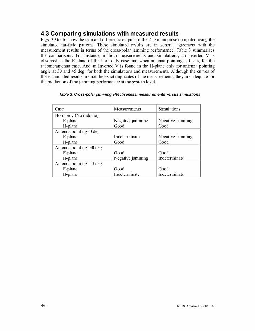
4.3 Comparing simulations with measured results Figs. 39 to 46 show the sum and difference outputs of the 2-D monopulse computed using the simulated far-field patterns. These simulated results are in general agreement with the measurement results in terms of the cross-polar jamming performance. Table 3 summarizes the comparisons. For instance, in both measurements and simulations, an inverted V is observed in the E-plane of the horn-only case and when antenna pointing is 0 deg for the radome/antenna case. And an Inverted V is found in the H-plane only for antenna pointing angle at 30 and 45 deg, for both the simulations and measurements. Although the curves of these simulated results are not the exact duplicates of the measurements, they are adequate for the prediction of the jamming performance at the system level.

Table 3. Cross-polar jamming effectiveness: measurements versus simulations

Case Measurements Simulations Horn only (No radome): E-plane H-plane

Negative jamming Good


Antenna pointing=0 deg E-plane H-plane

Indeterminate Good



Good Negative jamming

Good Indeterminate


Good Indeterminate

Good Indeterminate


(A) Simulated Co-polar Monopulse Patterns

0.0

0.2

0.4

0.6

0.8

1.0

1.2

80 82 84 86 88 90 92 94 96 98 100

Scan angle [deg]

Nor

mal

ized

am

plitu

de


E-plane, Theta-pol

(B) Simulated Cross-polar Monopulse Patterns

0.00

0.05

0.10

0.15

0.20

0.25

0.30

0.35

0.40

0.45

0.50

80 82 84 86 88 90 92 94 96 98 100

Scan angle [deg]

Nor

mal

ized

am

plitu

de


E-plane, Phi-pol

Figure 39. Simulated E-plane Monopulse patterns of the X-band Horn



0.0

0.2

0.4

0.6

0.8

1.0

1.2

-20 -15 -10 -5 0 5 10 15 20

Scan angle [deg]

Nor

mal

ized

am

plitu


H-plane, Theta-pol


0.0

0.2

0.4

0.6

0.8

1.0

1.2

-20 -15 -10 -5 0 5 10 15 20

Scan angle [deg]

Mor

mal

ized

am

plitu

de


H-plane, Phi-pol

Figure 40. Simulated H-plane Monopulse patterns of the X-band Horn



0.0

0.2

0.4

0.6

0.8

1.0

1.2

60 70 80 90 100 110 120

Scan Angle [deg]

Nor

mal

ized

Am

plitu


E-plane, Theta-pol


0.0

0.2

0.4

0.6

0.8

1.0

1.2

60 70 80 90 100 110 120

Scan Angle [deg]

Nor

mal

ized

am

plitu

de


E-plane, Phi-pol

Figure 41. Simulated E-plane patterns antenna pointing angle=0 deg



0.0

0.2

0.4

0.6

0.8

1.0

1.2

-30 -20 -10 0 10 20 30

Scan Angle [deg]

Nor

mal

ized

am

plitu


H-plane, Theta-pol

(B) Simulated Cross Polar Monopulse Patterns

0.0

0.2

0.4

0.6

0.8

1.0

1.2

-30 -20 -10 0 10 20 30

Scan Angle [deg]

Nor

mal

ized

am

plitu

de


H-Plane, Phi-pol

Figure 42. Simulated H-plane patterns with antenna pointing angle=0 deg



0.0

0.2

0.4

0.6

0.8

1.0

1.2

60 70 80 90 100 110 120

Scan Angle [deg]

Nor

mal

ized

am

plitu

de


E-plane, Thet a-pol


0.0

0.2

0.4

0.6

0.8

1.0

1.2

60 70 80 90 100 110 120

Scan Angle [deg]

Nor

mal

ized

am

plitu

de


E-plane, phi-pol

Figure 43. Simulated E-plane patterns with antenna pointing angle=30 deg



0.0

0.2

0.4

0.6

0.8

1.0

1.2

-60 -50 -40 -30 -20 -10 0

Scan Angle [deg]

Nor

mal

ized

am

plitu

de


H-plane, Thet a-pol

(B) Simulated Cross Polar Monopulse Patterns

0.0

0.2

0.4

0.6

0.8

1.0

1.2

-60 -50 -40 -30 -20 -10 0

Scan angle [deg]

Nor

mal

ized

am

plitu

de


H-plane, Phi-pol




0.0

0.2

0.4

0.6

0.8

1.0

1.2

60 70 80 90 100 110 120

Scan Angle [deg]

Nor

mal

ized

am

plitu


E-plane, Theta-pol


0.0

0.2

0.4

0.6

0.8

1.0

1.2

60 70 80 90 100 110 120

Scan angle [deg]

Nor

mal

ized

am

plitu

de


E-plane, Theta-pol

Figure 45. Simulated E-plane patterns with antenna pointing angle=45 deg



0.0

0.2

0.4

0.6

0.8

1.0

1.2

-75 -65 -55 -45 -35 -25 -15

Scan Angle [deg]

Nor

mal

ized

am

plitu

de


H-plane, Theta-pol


0.0

0.2

0.4

0.6

0.8

1.0

1.2

-75 -65 -55 -45 -35 -25 -15

Scan Angle [deg]

Nor

mal

ized

am

plitu

de


H-plane, Phi-pol



4.4 Tracking errors A jammer using a cross polarization technique transmits a signal with a polarization near orthogonal to the reference polarization at which the tracking radar operates. The total tracking error at the output of the monopulse receiver is a sum of the error signals due to the reference echo and the cross-polar jamming signal. Since the polarization of the jamming signal is not exactly orthogonal to that of the reference polarization, it contributes to both the co-polar and cross-polar components. Therefore, the total tracking error at the monopulse output can be expressed as: ββ cos)sin1(_ ⋅⋅+⋅+⋅= ΣΣ kCxkCoErrSum ββ cos)sin1(_ ⋅⋅+⋅+⋅= ∆∆ kCxkCoErrDif

ErrSumErrDifErrorTracking

__

=

Where Sum_Err =Error signal at the output of the SUM channel Dif_Err = Error signal at the output of the DIFFERENCE channel

ΣCo =Monopulse SUM output due to the co-polar echo ΣCx =Monopulse SUM output due to cross-polar jamming signal

∆Co =Monopulse DIFFERENCE output due to the co-polar echo signal ∆Cx =Monopulse DIFFERENCE output due to cross-polar jamming signal k =Cross-polar amplitude factor (as defined in section 4.1)

β =Polarization angle of the jamming signal (0 deg = orthogonal polarization) The tracking errors are calculated using the measured far-field patterns of the PHA with and without the radome. Figs. 47 to 50 show the calculated tracking errors signals for various antenna-pointing angles and amplitude factor k varying between 0 and 10. For these computations, the polarization angle β is set at orthogonal polarization (0 deg). Table 4 summarizes the maximum tracking errors for all cases.

Table 4. Tracking Errors

Case Tracking Error

in E-plane Tracking Error in H-plane

Horn only (No radome): 0.0 deg 2.5 deg

Antenna pointing=0 deg 0.0 deg 3.5 deg

Antenna pointing=30 deg 4.0 deg 0.0 deg

Antenna pointing=45 deg 1.2 deg Indeterminate


As summarized in Table 4, in the no-radome case, no error signal can be induced by a cross-polarized signal in the E-plane. Therefore, the tracking response cannot be perturbed by a cross-polar jamming signal directed along the E-plane. This is true regardless of the amplitude of the cross-polar jamming signal. When a jamming signal is arriving along the H-plane a tracking error of up to 2.5 deg can result when the cross-polar amplitude factor varies from 1 to 10. A similar scenario occurs in the radome/antenna case when the antenna is pointed at the tip (antenna pointing angle is 0 deg). However, a larger tracking error of up to 3.5 deg is observed in the H-plane. When the antenna-pointing angle is at 30 deg, a tracking error can only be induced when the jamming signal is arriving along the E-plane. In this case, a tracking error of nearly 4 deg is observed. When the antenna-pointing angle is 45 deg, the jamming signal is no longer effective, only a small tracking error of up to 1.2 deg is observed if the jamming signal arrives in the E-plane.


(A) Feed Horn E-plane

0.00

0.05

0.10

0.15

0.20

0.25

0.30

0.35

0.40

80 82 84 86 88 90 92 94 96 98 100

Scan angle [deg]

Nor

mal

ized

am

plitu

deK=0.0

K=0.1

K=0.2

K=0.5

K=0.8

K=1.0

K=2.0

K=4.0

K=5.0

K=10.0

DFL DataPol angle=0.0

K=00

K=10.

(B) Feed Horn H-plane

0.00

0.05

0.10

0.15

0.20

0.25

0.30

80 82 84 86 88 90 92 94 96 98 100

Scane angle [deg]

Nor

mal

ized

am

plitu

de

K=0.0

K=0.1

K=0.2

K=0.5

K=0.8

K=1.0

K=2.0

K=4.0

K=5.0

K=10.0

DFL dataPol angle=0.0

K=0.0

K=10.

Figure 47. Tracking errors without radome


(A) E-plane, Antenna poitning angle= 0 deg

0.00

0.05

0.10

0.15

0.20

0.25

80 82 84 86 88 90 92 94 96 98 100

Scan angle [deg]

Nor

mal

ized

am

plitu

deK=0.0

K=0.1

K=0.2

K=0.5

K=0.8

K=1.0

K=2.0

K=4.0

K=5.0

K=10.0

DFL Radome H-polPol angle=0 degAnt angle=0 deg

K=0

K=10.0

(B) H-plane, Antenna pointing angle=0 deg

0.00

0.02

0.04

0.06

0.08

0.10

0.12

0.14

0.16

0.18

0.20

80 82 84 86 88 90 92 94 96 98 100

Scan angle [deg]

Nor

mal

ized

am

plitu

de

K=0.0

K=0.1

K=0.2

K=0.5

K=0.8

K=1.0

K=2.0

K=4.0

K=5.0

K=10.0

DFL Radome V-polpol angle=0.0A t l 0 d

K=0.0

K=10

Figure 48. Tracking errors with antenna pointing angle=0 deg


(A) E-plane, Antenna pointing angle=30 deg

0.00

0.05

0.10

0.15

0.20

0.25

80 82 84 86 88 90 92 94 96 98 100

Scan angle [deg]

NO

rmal

ized

am

plitu

deK=0.0

K=0.1

K=0.2

K=0.5

K=0.8

K=1.0

K=2.0

K=4.0

K=5.0

K=10.0

DFL Radome H-polPol angle=0.0 degAnt angle=30.0 deg

K=0.0

K=10.


0.00

0.05

0.10

0.15

0.20

0.25

0.30

0.35

0.40

80 82 84 86 88 90 92 94 96 98 100

Scan angle [deg]

Nor

mal

ized

am

plitu

de

K=0.0

K=0.1

K=0.2

K=0.5

K=0.8

K=1.0

K=2.0

K=4.0

K=5.0

K=10.0

DFL Radome V-polPol angle=0.0 degAnt angle=30.0 deg

K=10.

K=0.0



(A) E-plane, Antenna pointing angle=45 deg

0.00

0.05

0.10

0.15

0.20

0.25

0.30

80 82 84 86 88 90 92 94 96 98 100

Scan angle [deg]

Nor

mal

ized

am

plitu

de

K=0.0

K=0.1

K=0.2

K=0.5

K=0.8

K=1.0

K=2.0

K=4.0

K=5.0

K=10.0

DFL Radome H-polPol angle=0.0 degAnt angle=45 deg

K=0.0

K=10.0


0.00

0.05

0.10

0.15

0.20

0.25

0.30

0.35

80 82 84 86 88 90 92 94 96 98 100

Scan angle [deg]

Nor

mal

ized

am

plitu

de

K=0.0

K=0.1

K=0.2

K=0.5

K=0.8

K=1.0

K=2.0

K=4.0

K=5.0

K=10.0

DFL Radome V-polPol angle=0.0 degAnt angle=45 deg

K=0.0

K=10.0



Up to this point, all tracking errors were calculated on the assumption that the relative polarization angle between the received echo and the jamming signal were orthogonal to each other. In reality, it is not feasible to maintain such condition at all time. To assess the non-ideal scenario, an experiment has been conducted to investigate the effect of polarization angle ( 0≠β ) on tracking errors.

As defined previously, the polarization angle β is the deviation angle from the ideal orthogonal condition between the received echo (co-polar) and the jamming signal (cross-polar). The following experiment is conducted using the measured H-plane pattern with the antenna-pointing angle=0 deg. Figs. 51 to 57 show the computed tracking errors for polarization angles between 0 to 90 deg, with the amplitude factor K between 0 and 10. Evidently, the maximum tracking error reduces rapidly from 3.5 deg to 0 deg as the polarization angle increases from 0 to 90 deg. In fact, the jamming signal is no longer effective once the polarization reaches 30 deg to 45 deg as shown in Figs. 53 and 54.

Tracking Errors

0.00

0.05

0.10

0.15

0.20

0.25

80 82 84 86 88 90 92 94 96 98 100

Scan angle [deg]

Nor

mal

ized

am

plitu

de

K=0.0

K=0.1

K=0.2

K=0.5

K=0.8

K=1.0

K=2.0

K=4.0

K=5.0

K=10.0

DFL Radome V-polpol angle=0.0Ant angle =0 deg

K=0.0

K=10.0

Figure 51. Tracking errors with polarization angle=0 deg


Tracking Errors

0.00

0.02

0.04

0.06

0.08

0.10

0.12

0.14

0.16

0.18

0.20

80 82 84 86 88 90 92 94 96 98 100

Scan angle [deg]

Nor

mal

ized

am

plitu

deK=0.0

K=0.1

K=0.2

K=0.5

K=0.8

K=1.0

K=2.0

K=4.0

K=5.0

K=10.0


K=0.0

K=10.0


Tracking Errors

0.00

0.02

0.04

0.06

0.08

0.10

0.12

0.14

0.16

0.18

0.20

80 82 84 86 88 90 92 94 96 98 100

Scan angle [deg]

Nor

mal

ized

am

plitu

de

K=0.0

K=0.1

K=0.2

K=0.5

K=0.8

K=1.0

K=2.0

K=4.0

K=5.0

K=10.0


K=0.0

K=10.



Tracking Errors

0.00

0.02

0.04

0.06

0.08

0.10

0.12

0.14

0.16

0.18

0.20

80 82 84 86 88 90 92 94 96 98 100

Scan angle [deg]

Nor

mal

ized

am

plitu

deK=0.0

K=0.1

K=0.2

K=0.5

K=0.8

K=1.0

K=2.0

K=4.0

K=5.0

K=10.0


K=0.0

K=10.0


Tracking Errors

0.00

0.02

0.04

0.06

0.08

0.10

0.12

0.14

0.16

0.18

0.20

80 82 84 86 88 90 92 94 96 98 100

Scan angle [deg]

Nor

mal

ized

am

plitu

de

K=0.0

K=0.1

K=0.2

K=0.5

K=0.8

K=1.0

K=2.0

K=4.0

K=5.0

K=10.0


K=0.0

K=10.0



Tracking Errors

0.00

0.02

0.04

0.06

0.08

0.10

0.12

0.14

0.16

0.18

0.20

80 82 84 86 88 90 92 94 96 98 100

Scan angle [deg]

Nor

mal

ized

am

plitu

de

K=0.0

K=0.1

K=0.2

K=0.5

K=0.8

K=1.0

K=2.0

K=4.0

K=5.0

K=10.0


K=0.0

K=10.0


Tracking Errors

0.00

0.02

0.04

0.06

0.08

0.10

0.12

0.14

0.16

0.18

0.20

80 82 84 86 88 90 92 94 96 98 100

Scan angle [deg]

Nor

mal

ized

Am

plitu

de

K=0.0

K=0.1

K=0.2

K=0.5

K=0.8

K=1.0

K=2.0

K=4.0

K=5.0

K=10.0


K=0.0 to 10.0



Intuitively, a tracking antenna with a higher relative level of cross-polar patterns is likely to be more susceptible to the cross-polar jamming. Questions of particular interest for this study are: how does the relative cross-polar level (compared to the co-polar peak) affect the tracking error and what is the minimum level of cross-polar component required in order for the jamming signal to be effective. To answer these questions, tracking errors are computed at different polarization angles for various cross-polar jamming signal levels for different relative cross-polar (Cx/Co) patterns. These results are summarized in Fig. 58. From this plot, one can estimate the maximum allowable polarization angle for a given maximum tracking error and cross-polar signal. For instance, given a cross-polar pattern with a peak value at –20 dB compared to the peak of the reference echo signal, the maximum polarization angle is 15 deg for a maximum tracking error of 3 deg. It is also evident from this plot that the cross-polar jamming signal is not effective if the peak value of the cross-polar pattern is below –30 dB from the peak of the reference echo.

Monopulse Tracking Error versus Polarization angle

0

1

2

3

4

5

6

0 5 10 15 20 25 30 35 40 45

Polarization angle [deg]

Max

Tra

ckin

g Er

ror [

deg]

Cx/Co= -20 dB

Cx/Co= -30dB

Cx/Co= -40

*Cross-polar jamming signal 0.0 to +20.0dB (K=0.0 to 10.0) compared to co-polar signal at the received antenna

Figure 58. Tracking errors versus polarization angles


5. Discussion The proposed high-frequency method works well for prediction of the co-polar patterns of a radome-enclosed antenna. The accuracy is satisfactory within the main beam, except for the case where the radome shape is highly irregular or the geometry is changing rapidly such as the tip of a tangent ogive radome. The cross-polar patterns are more difficult both in terms of simulations and measurements. However, the current method produces results that are satisfactory for quantitative analyses of jamming performance at the system level. A more rigorous method is required to further improve modeling of the cross-polar patterns, especially for radome with highly irregular geometry. One such method being investigated is combination of the current method in conjunction with FEM. For instance, FEM can be used to model the tip of the ogive radome when ray tracing is used for the smooth surfaces. The jamming performance of a 2-D monopulse system was analyzed in the two principal planes, for various antenna-pointing angles. Results show that a missile’s radome affects jamming performance of monopulse tracking significantly. Depending on the shape, material of the radome and the incidence angle, a jamming signal may or may not be effective. These results are based on pyramidal horn monopulse antenna. A more commonly used antenna for monopulse applications is a reflector. How and what the differences are in the cross-polar characteristics of a reflector-type monopulse antenna and a PHA monopulse antenna have yet to be investigated in further studies. In addition, the current study is limited to the two principal planes only. Coupling between co-polar and cross-polar pattern is more intricate in the off-principal-plane angles. The effect of the radome by a jamming signal in these off-principal-plane angles has yet to be studied. Results of this study have shown that a tracking monopulse antenna must possess a null near the electrical boresight of the cross-polar pattern to be susceptible to a cross-polar jamming. It is therefore possible to counter the cross-polar jamming by incorporating features into the radome/antenna to minimize this characteristic. At the least, one may reduce the overall coverage angles of the cross-polar jamming. For instance, a frequency selective surface (FSS) can be incorporated into the inside surface of the radome to suppress or modify the incoming cross-polar signal. These effects can also be modeled using this simulation tool in the future studies.


6. Conclusions A general EM analysis procedure has been implemented for analyses of radome-enclosed antennas. The high-frequency approximation method is based on a hybrid of the method-of-moments (MOM) and EM ray tracing. Through near-field analyses, this method allows accurate modeling of the monopulse feed structure. This method works well for radome with smooth surfaces. A tangent ogive radome model was manufactured and measured at the DFL/CSA. The predictions of co-polar patterns compare well with measurements, except when the antenna is pointing directly at the tip of the radome. Predictions of cross-polar patterns do not compare as well as the co-polar cases, however, are sufficient for quantitative analyses of jamming performance at the system level. A more rigorous solution is being developed to further improve accuracy of the prediction in this aspect. Effectiveness of cross-polar jamming was analyzed using the measured and simulated radiation patterns. Results show that a typical missile radome changes the co-polar and cross-polar patterns significantly and the effect varies with the pointing angle of the antenna. A monopulse system is susceptible to cross-polar jamming only when a null appears near the electrical boresight of the cross-polar pattern. Yet, a radome-enclosed antenna does not possess this characteristic for all antenna-pointing angles since the radome modifies radiation patterns of the feed antenna differently at different antenna-pointing angles. As a result, a radome-enclosed monopulse system is in general not 100% susceptible to a cross-polar jamming. Results showed that the susceptibility is partial and depends on various factors, such as the type of feed antenna, radome materials, and the incidence angle. Results also show that the effectiveness of cross-polar jamming diminishes rapidly when the amplitude ratio of the cross-polar to co-polar field (Cx/Co) of the monopulse antenna is below –30 dB, assuming the cross-polar signal is perfectly orthogonal to the reference echo signal. If the polarization of the jamming signal is more than 30 deg off that of the reference echo, the jamming signal is no longer considered effective. This implies that the polarization angle of a dynamic cross-polar jamming signal need not go beyond 30 deg. Finally, the model of this study is based on PHA monopulse antenna. Validity of the results of this study to other types of monopulse antennas such as a reflector-type antenna has yet to be verified in further studies.


References

Radome Analysis

[1] Paris, D.T. (1970). Computer-aided radome analysis. IEEE Trans. Antennas & propagations, AP-18 (1), 7-15.

[2] Wu, D.C.F. and Rudduck, R.C. (1974). Plane wave spectrum-surface integration

technique for radome analysis. IEEE Trans. Antenna & propagation, AP-22, 497-500.

[3] Huddleston, G.K., Bassett, H.L., and Newton, J.M. Parametric investigation of

radome analysis methods: Salient results. Defense technical report, AFSR-TR-81-0459.

[4] Burks, D.G., Graf, E.R., and Fahey, M.D. (1982). A high-frequency analysis of

radome-induced radar pointing error. IEEE Trans. Antenna & Propagation, AP-30, 947-955.

[5] Kozakoff, D.J. (1997). Analysis of radome-enclosed antennas. Artech House, Boston. [6] Graf, E.R. and Burks, D.G. (1979). Investigation of complex angle processing to

reduce induced angle pointing errors. (AU-EE-0022-Final, Defense Technical Information Center accessing number: ADA085263). U.S. Army Missile Command.

[7] Lee, S.W., Jamnejad, V., Sheshadri, M.S., Mittra, R. (1980). Analysis of antenna

radomes by ray techniques, part I: point source. (UIEM-80-2, UILU-ENG-80-2542, Defense Technical Information Center accessing number: ADA085329). Naval Air Systems Command.

[8] Tavis, M. (1971). A three-dimensional ray-tracing method for the calculation of

radome boresight error and antenna pattern distortion. (TOR-0059(S6860)-2, SAMSO TR-71-210, Defense Technical Information Center accessing number: AD729811). Air Force Systems Command.

[9] Wilson, K.S. (1994). Polarization sensitivity of monopulse radar boresight error

induced by large, ogive radomes. (Thesis: AFIT/GE/ENG/94D-31, Defense Technical Information Center accessing number: ADA28925). Air force institute of technology.

[10] Overfelt, P.L. (1985). Radome analysis and design capabilities of the RF and

microwave technology branch. (NWC TP 6636, Defense Technical Information Center accessing number: AD-A156 662). Naval Weapons Center.

[11] Huddlestone, G.K., Bassett, H.L. and Newton, J.M. (1981). Parametric investigation

of radome analysis methods: salient results. (AFOSR-TR-81-0459, Defense Technical Information Center accessing number: AD-A099181). U.S. Air force.


[12] Huddlestone, G.K., Bassett, H.L. and Newton, J.M. (1981). Parametric investigation of radome analysis methods: Computer-aided radome analysis using geometrical optics and Lorentz reciprocity. (AFOSR-TR-81-0460, Defense Technical Information Center accessing number: AD-A099182). U.S. Air force.

[13] Kim., J.J. and Kesler, O.B. (1999). Performance analysis of radar antenna systems.

IEEE Aerospace & Electronic Systems Magazine, 14(6), 38-42. [14] Balanis, C.A. (1989). Advanced Engineering Electromagnetics. John Wiley & Sons,

New York, NY.

Cross-Polarization & Jammers

[15] Ludwig, A.C. (1973). The definition of cross polarization. IEEE Trans. Antennas Propagation, AP-21, 116-119.

[16] Symons, F.W. (1997). Cross polarization jamming of monopulse radar. (DREO-TM-

17/97). Defence Research Establishment Ottawa. [17] Lees, M.L. (1976). Cross-polarisation tracking errors on a linearly polarized

monopulse radar. In Monitor-Proceedings of the IREE Augt, 306-310.

[18] Neri, F. (1991). New Technologies in self-protection jammers. Journal of electronic defense, July, 55-58.

[19] Lo, Y.T. and Lee, S.W. (1993). Antenna Handbook, Vol.(I), Fundamentals and

Mathematical Techniques. Chapman & Hall, New York, NY.

Monopulse Radars

[20] Leonov, A.I. and Fomichev, K.I. (1986). Monopulse Radar. Artech House, Norwood, MA.

[21] Sherman, S.M. (1984). Monopulse principles and techniques. Artech House, Dedham,

MA.

Method of Moments

[22] Stutzman, W.L. and Thiele, G. A. (1981). Antenna Theory and Design. John Wiley & Sons, New York.

[23] Hwu, S.U. and Wilton, D.R. (1987). JUNCTION: Electromagnetic scattering and

radiation by arbitrary configurations of conducting bodies and wires. Applied Electromagnetics Laboratory Technical Report Number 87-17, University of Houston, TX.

[24] Balanis, C.A. (1982). Antenna Theory: Analysis and Design. Harper & Row, New

York.


[25] Burke, G.J. and Poggio, A.J. (1977). Numerical Electromagnetic Code (NEC) — Method of Moments. Technical Document 116, Naval Ocean Systems Center, San Diego, CA.


List of abbreviations/acronyms

AI Aperture integration

DND Department of National Defence

DRDC Defence Research & Development Canada

MOM Method of moments

FDTD Finite difference time domain

FEM Finite element method

PHA Pyramidal horn antenna

DFL David Florida Lab.

CSA Canadian Space Agency

CRC Communications Research Centre Canada

NEC Numerical Electromagnetic Code

EM Electromagnetic

IPD Insertion phase delay

TE Transverse electric

TM Transverse magnetic

B DRDC Ottawa TR 2003-153

Annex A: Measured radiation patterns

(A) H-Plane patterns.

Transmit polarization = Vertical

Receive co-polar polarization=Vertical

Receive cross-polar polarization=Horizontal

DRDC Ottawa TR 2003-153 C

(B) E-plane Patterns

Transmit polarization = Vertical

Receive co-polar polarization=Horizontal

Receive cross-polar polarization=Vertical

D DRDC Ottawa TR 2003-153

( C) Standard Gain Horn

DRDC Ottawa TR 2003-153 E

Annex B: Comparisons of squint-beam patterns

UNCLASSIFIED SECURITY CLASSIFICATION OF FORM

(highest classification of Title, Abstract, Keywords)

DOCUMENT CONTROL DATA (Security classification of title, body of abstract and indexing annotation must be entered when the overall document is classified)

1. ORIGINATOR (the name and address of the organization preparing the document. Organizations for whom the document was prepared, e.g. Establishment sponsoring a contractor’s report, or tasking agency, are entered in section 8.)

Defence R&D Canada - Ottawa, 3701 Carling Avenue, Ottawa, Ontario, K1A 0Z4

2. SECURITY CLASSIFICATION (overall security classification of the document,

including special warning terms if applicable) UNCLASSIFIED

3. TITLE (the complete document title as indicated on the title page. Its classification should be indicated by the appropriate abbreviation (S,C or U) in parentheses after the title.)

Modeling of Cross Polarization Tracking Errors of Radome-Enclosed Monopulse Systems (U)

4. AUTHORS (Last name, first name, middle initial)

Foo, Senglee; Louie Aloisius; Kashyap, Satish

5. DATE OF PUBLICATION (month and year of publication of document)

March 2003

6a. NO. OF PAGES (total containing information. Include Annexes, Appendices, etc.)

54

6b. NO. OF REFS (total cited in document)

24

7. DESCRIPTIVE NOTES (the category of the document, e.g. technical report, technical note or memorandum. If appropriate, enter the type of report, e.g. interim, progress, summary, annual or final. Give the inclusive dates when a specific reporting period is covered.)

Technical Report

8. SPONSORING ACTIVITY (the name of the department project office or laboratory sponsoring the research and development. Include the address.)

DRDC Ottawa

9a. PROJECT OR GRANT NO. (if appropriate, the applicable research and development project or grant number under which the document was written. Please specify whether project or grant)

9b. CONTRACT NO. (if appropriate, the applicable number under which the document was written)

10a. ORIGINATOR’S DOCUMENT NUMBER (the official document number by which the document is identified by the originating activity. This number must be unique to this document.)

DRDC Ottawa TM 2003-153

10b. OTHER DOCUMENT NOS. (Any other numbers which may be assigned this document either by the originator or by the sponsor)

11. DOCUMENT AVAILABILITY (any limitations on further dissemination of the document, other than those imposed by security classification) ( x ) Unlimited distribution ( ) Distribution limited to defence departments and defence contractors; further distribution only as approved ( ) Distribution limited to defence departments and Canadian defence contractors; further distribution only as approved ( ) Distribution limited to government departments and agencies; further distribution only as approved ( ) Distribution limited to defence departments; further distribution only as approved ( ) Other (please specify):

12. DOCUMENT ANNOUNCEMENT (any limitation to the bibliographic announcement of this document. This will normally correspond to

the Document Availability (11). However, where further distribution (beyond the audience specified in 11) is possible, a wider announcement audience may be selected.)

Full unlimited announcement.

UNCLASSIFIED

SECURITY CLASSIFICATION OF FORM DDCCDD0033 22//0066//8877

UNCLASSIFIED SECURITY CLASSIFICATION OF FORM

13. ABSTRACT ( a brief and factual summary of the document. It may also appear elsewhere in the body of the document itself. It is highly desirable that the abstract of classified documents be unclassified. Each paragraph of the abstract shall begin with an indication of the security classification of the information in the paragraph (unless the document itself is unclassified) represented as (S), (C), or (U). It is not necessary to include here abstracts in both official languages unless the text is bilingual).

A cross-polarized signal transmitted by a jammer passes through a protective radome before reaching the aperture of a missile antenna. As a result, the actual co-polar and cross-polar tracking response of the monopulse system changes and varies with the relative antenna-pointing angle. This study describes a systematic EM procedure for the prediction of the co-polar and cross-polar radiation patterns of radome-enclosed antennas. Both the measured and predicted results show that the presence of a radome significantly affects the susceptibility of a monopulse tracking system to the cross-polar jamming. In fact, the effectiveness of the cross-polar jamming depends on various factors such as the incidence angle, polarization angle, the shape and material of the radome, and the type of the antenna. Results of this study show that the cross-polar jamming in general does not have 100% of coverage angles. It is effective only in certain incidence angles and when the polarization angle is less than 30 deg. In some incidence angles, cross-polar jamming is deemed to be effective

14. KEYWORDS, DESCRIPTORS or IDENTIFIERS (technically meaningful terms or short phrases that characterize a document and could be helpful in cataloguing the document. They should be selected so that no security classification is required. Identifiers such as equipment model designation, trade name, military project code name, geographic location may also be included. If possible keywords should be selected from a published thesaurus. e.g. Thesaurus of Engineering and Scientific Terms (TEST) and that thesaurus-identified. If it is not possible to select indexing terms which are Unclassified, the classification of each should be indicated as with the title.)

Radome, Monopulse antenna, Cross polarization, Jamming, Tracking error

UNCLASSIFIED

SECURITY CLASSIFICATION OF FORM

Defence R&D Canada

Canada’s leader in defenceand national security R&D

Chef de file au Canada en R & Dpour la défense et la sécurité nationale

R & D pour la défense Canada

www.drdc-rddc.gc.ca

Date post:	04-Apr-2018
Category:	Documents
Upload:	dangkiet
View:	224 times
Download:	3 times

Modeling of Cross Polarization Tracking Errors of...

Documents