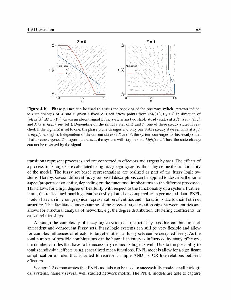
Modeling of Dynamic Systems with Petri Nets and Fuzzy Logic

Modeling of Dynamic Systems withPetri Nets and Fuzzy Logic

Lukas Windhager

Dissertationan der Fakultat fur Mathematik, Informatik und Statistik

der Ludwig–Maximilians–UniversitatMunchen

vorgelegt vonLukas Windhager

aus Bad Ischl, Osterreich

Munchen, den 25.04.2013

Erstgutachter: Prof. Dr. Ralf ZimmerZweitgutachter: Prof. Dr. Fabian TheisTag der mundlichen Prufung: 19.04.2013

Eidesstattliche Versicherung(Siehe Promotionsordnung vom 12.07.11, § 8, Abs. 2 Pkt. .5.)

Hiermit erklare ich an Eides statt, dass die Dissertation von mirselbststandig und ohne unerlaubte Beihilfe angefertigt wurde.

Windhager, LukasName, Vorname

Ort, Datum Unterschrift Doktorand/in

vi

Table of Contents

Zusammenfassung/Abstract xv

Introduction 1

1 Introduction 31.1 Models of Biological Systems . . . . . . . . . . . . . . . . . . . . . . . . . . . 3

1.1.1 Abstraction and Representation . . . . . . . . . . . . . . . . . . . . . . 51.1.2 Reverse-Engineering . . . . . . . . . . . . . . . . . . . . . . . . . . . . 6

1.2 Computational Modeling in Bioinformatics . . . . . . . . . . . . . . . . . . . . 71.2.1 Discrete Logic Models . . . . . . . . . . . . . . . . . . . . . . . . . . . 81.2.2 Ordinary Differential Equations Models . . . . . . . . . . . . . . . . . . 10

1.3 Qualitative Knowledge . . . . . . . . . . . . . . . . . . . . . . . . . . . . . . . 121.4 Our Contribution . . . . . . . . . . . . . . . . . . . . . . . . . . . . . . . . . . 13

I Modeling with Petri Nets and Fuzzy Logic 15

2 Fuzzy Sets Describe States of Biological Entities 172.1 Common Shapes of Fuzzy Sets . . . . . . . . . . . . . . . . . . . . . . . . . . . 20

2.1.1 Triangle-like Fuzzy Sets . . . . . . . . . . . . . . . . . . . . . . . . . . 202.1.2 Trapezoid-like Fuzzy Sets . . . . . . . . . . . . . . . . . . . . . . . . . 222.1.3 Gaussian-like Fuzzy Sets . . . . . . . . . . . . . . . . . . . . . . . . . . 232.1.4 Unbounded Fuzzy Sets . . . . . . . . . . . . . . . . . . . . . . . . . . . 23

2.2 The Design of Fuzzy Sets . . . . . . . . . . . . . . . . . . . . . . . . . . . . . . 242.3 Discussion . . . . . . . . . . . . . . . . . . . . . . . . . . . . . . . . . . . . . . 25

3 Fuzzy Logic Systems Give Functionality to Interactions 293.1 A Numerical Example . . . . . . . . . . . . . . . . . . . . . . . . . . . . . . . 333.2 Fuzzy Logic Systems Can Approximate Common Functions . . . . . . . . . . . 36

3.2.1 Hill and Michaelis-Menten Kinetics . . . . . . . . . . . . . . . . . . . . 363.2.2 Mass-Action Kinetics . . . . . . . . . . . . . . . . . . . . . . . . . . . . 393.2.3 Logical Gates . . . . . . . . . . . . . . . . . . . . . . . . . . . . . . . . 40

viii TABLE OF CONTENTS

3.3 Discussion . . . . . . . . . . . . . . . . . . . . . . . . . . . . . . . . . . . . . . 42

4 Joining Petri Nets and Fuzzy Logic: PNFL Modeling 454.1 Definition of a PNFL Model . . . . . . . . . . . . . . . . . . . . . . . . . . . . 45

4.1.1 Simulation of PNFL Models . . . . . . . . . . . . . . . . . . . . . . . . 464.1.2 Modeling Multiple Effectors . . . . . . . . . . . . . . . . . . . . . . . . 484.1.3 Semi-Continuous and Semi-Discrete Modeling . . . . . . . . . . . . . . 51

4.2 PNFL Models Can Mimic Common Network Motifs . . . . . . . . . . . . . . . 524.2.1 Feed-Forward Loop . . . . . . . . . . . . . . . . . . . . . . . . . . . . 524.2.2 Negative Feedback Oscillator . . . . . . . . . . . . . . . . . . . . . . . 554.2.3 Positive Feedback Toggle Switch . . . . . . . . . . . . . . . . . . . . . 584.2.4 Positive Feedback One-Way Switch . . . . . . . . . . . . . . . . . . . . 60

4.3 Discussion . . . . . . . . . . . . . . . . . . . . . . . . . . . . . . . . . . . . . . 60

5 A Model of a Cell-Free Transcription/Translation System 655.1 Experimental Methods and Acquired Data . . . . . . . . . . . . . . . . . . . . . 675.2 Computational Models of the Cell-Free System . . . . . . . . . . . . . . . . . . 69

5.2.1 The ODE Model . . . . . . . . . . . . . . . . . . . . . . . . . . . . . . 695.2.2 The PNFL Model . . . . . . . . . . . . . . . . . . . . . . . . . . . . . . 71

5.3 Selecting Models for Consumption and Decay . . . . . . . . . . . . . . . . . . . 725.3.1 Model Selection using the ODE Model . . . . . . . . . . . . . . . . . . 725.3.2 Model Selection using the PNFL Model . . . . . . . . . . . . . . . . . . 72

5.4 Discussion . . . . . . . . . . . . . . . . . . . . . . . . . . . . . . . . . . . . . . 74

II Reverse-Engineering of PNFL Models 81

6 A Genetic Algorithm for Reverse-Engineering 836.1 The Reverse-Engineering Algorithm . . . . . . . . . . . . . . . . . . . . . . . . 84

6.1.1 Valid PNFL Models . . . . . . . . . . . . . . . . . . . . . . . . . . . . 866.1.2 Mutation Operations . . . . . . . . . . . . . . . . . . . . . . . . . . . . 876.1.3 Simulation and Scoring . . . . . . . . . . . . . . . . . . . . . . . . . . . 896.1.4 Simulated Annealing and Acceptance Probability . . . . . . . . . . . . . 90

6.2 Evaluation of the Genetic Algorithm . . . . . . . . . . . . . . . . . . . . . . . . 916.2.1 DREAM4 in silico networks . . . . . . . . . . . . . . . . . . . . . . . . 916.2.2 Reference Networks Based on PNFL Models . . . . . . . . . . . . . . . 926.2.3 Reverse-Engineering Parameter and Evaluation Criteria . . . . . . . . . . 94

6.3 Discussion . . . . . . . . . . . . . . . . . . . . . . . . . . . . . . . . . . . . . . 95

7 Iterative Prediction of Large Network Models 997.1 Iterative Prediction Procedure . . . . . . . . . . . . . . . . . . . . . . . . . . . 1007.2 Data-Driven Restriction of Candidate Interactions . . . . . . . . . . . . . . . . . 1017.3 Evaluation Results . . . . . . . . . . . . . . . . . . . . . . . . . . . . . . . . . 102

Table of Contents ix

7.4 Discussion . . . . . . . . . . . . . . . . . . . . . . . . . . . . . . . . . . . . . . 104

8 Ensemble Approach for Reverse-Engineering 1118.1 Flaws of Ensemble Voting And How to Overcome Them . . . . . . . . . . . . . 1138.2 A Characteristic Interaction Set Extraction Approach . . . . . . . . . . . . . . . 1158.3 Evaluation Results . . . . . . . . . . . . . . . . . . . . . . . . . . . . . . . . . 1178.4 Discussion . . . . . . . . . . . . . . . . . . . . . . . . . . . . . . . . . . . . . . 121

Summary and Outlook 123

9 Summary and Outlook 1259.1 Petri Net and Fuzzy Logic Based Modeling . . . . . . . . . . . . . . . . . . . . 1259.2 Reverse-Engineering . . . . . . . . . . . . . . . . . . . . . . . . . . . . . . . . 1259.3 Outlook . . . . . . . . . . . . . . . . . . . . . . . . . . . . . . . . . . . . . . . 1269.4 Conclusion . . . . . . . . . . . . . . . . . . . . . . . . . . . . . . . . . . . . . 127

Appendix 129

A Ordinary Logic Reasoning and Fuzzy Logic - Theoretical Background 131A.1 Ordinary Logic Reasoning . . . . . . . . . . . . . . . . . . . . . . . . . . . . . 131

A.1.1 Modus Ponens . . . . . . . . . . . . . . . . . . . . . . . . . . . . . . . 131A.1.2 Ordinary Relations . . . . . . . . . . . . . . . . . . . . . . . . . . . . . 132A.1.3 Logic Implication . . . . . . . . . . . . . . . . . . . . . . . . . . . . . . 132

A.2 Fuzzy sets . . . . . . . . . . . . . . . . . . . . . . . . . . . . . . . . . . . . . . 133A.2.1 Operations on Fuzzy Sets . . . . . . . . . . . . . . . . . . . . . . . . . . 134

A.3 Fuzzy Logic Reasoning . . . . . . . . . . . . . . . . . . . . . . . . . . . . . . . 135A.3.1 Generalized Modus Ponens . . . . . . . . . . . . . . . . . . . . . . . . . 136A.3.2 Fuzzy Relations and Implication . . . . . . . . . . . . . . . . . . . . . . 136A.3.3 Fuzzy Logic Systems . . . . . . . . . . . . . . . . . . . . . . . . . . . . 138

Bibliography 141

x Table of Contents

List of Figures

1.1 Discretization issues . . . . . . . . . . . . . . . . . . . . . . . . . . . . . . . . 91.2 Obscured functionality . . . . . . . . . . . . . . . . . . . . . . . . . . . . . . . 101.3 A simple feed-forward motif . . . . . . . . . . . . . . . . . . . . . . . . . . . . 111.4 If-then rules describe processes . . . . . . . . . . . . . . . . . . . . . . . . . . . 121.5 Discretization of concentrations . . . . . . . . . . . . . . . . . . . . . . . . . . 13

2.1 Fuzzy sets describe states . . . . . . . . . . . . . . . . . . . . . . . . . . . . . . 182.2 Common shapes of fuzzy sets . . . . . . . . . . . . . . . . . . . . . . . . . . . . 212.3 Unbounded fuzzy sets . . . . . . . . . . . . . . . . . . . . . . . . . . . . . . . . 232.4 Fuzzy sets designed to represent functional properties . . . . . . . . . . . . . . . 252.5 Designing fuzzy sets . . . . . . . . . . . . . . . . . . . . . . . . . . . . . . . . 26

3.1 Fuzzy logic system flow-chart . . . . . . . . . . . . . . . . . . . . . . . . . . . 303.2 Example of a simple fuzzy logic system . . . . . . . . . . . . . . . . . . . . . . 343.3 Fuzzy logic systems approximate Hill and Michaelis-Menten functions . . . . . . 373.4 Fuzzy logic systems can mimic mass-action functions . . . . . . . . . . . . . . . 413.5 Fuzzy logic systems can mimic logic gates . . . . . . . . . . . . . . . . . . . . . 43

4.1 Example of a PNFL model . . . . . . . . . . . . . . . . . . . . . . . . . . . . . 474.2 Mutually independent effects . . . . . . . . . . . . . . . . . . . . . . . . . . . . 494.3 Integration of multiple effects . . . . . . . . . . . . . . . . . . . . . . . . . . . . 504.4 Semi-discrete modeling . . . . . . . . . . . . . . . . . . . . . . . . . . . . . . . 524.5 Modeling of slow state changes . . . . . . . . . . . . . . . . . . . . . . . . . . . 534.6 Feed-forward loop . . . . . . . . . . . . . . . . . . . . . . . . . . . . . . . . . 564.7 Negative feedback oscillator . . . . . . . . . . . . . . . . . . . . . . . . . . . . 594.8 Positive feedback toggle switch . . . . . . . . . . . . . . . . . . . . . . . . . . . 614.9 Positive feedback one-way switch . . . . . . . . . . . . . . . . . . . . . . . . . 624.10 One-way switch phase planes . . . . . . . . . . . . . . . . . . . . . . . . . . . . 63

5.1 The bacterial transcription/translation system . . . . . . . . . . . . . . . . . . . 665.2 Experimentally measured kinetics of mature GFP and mRNA . . . . . . . . . . . 765.3 PNFL model of the cell-free transcription/translation system . . . . . . . . . . . 775.4 GFP kinetics simulated using the PNFL model . . . . . . . . . . . . . . . . . . . 785.5 Comparison of mRNA and GFP kinetics . . . . . . . . . . . . . . . . . . . . . . 79

xii List of Figures

6.1 Pseudocode of the reverse-engineering algorithm . . . . . . . . . . . . . . . . . 856.2 Pseudocode for converting a PNFL model to a directed graph . . . . . . . . . . . 856.3 Rule bases for random PNFL models . . . . . . . . . . . . . . . . . . . . . . . . 936.4 Genetic algorithm evaluation results . . . . . . . . . . . . . . . . . . . . . . . . 96

7.1 Pseudocode of the iterative procedure . . . . . . . . . . . . . . . . . . . . . . . 1007.2 Evaluation of interaction scores . . . . . . . . . . . . . . . . . . . . . . . . . . . 1037.3 Comparison to score based predictions. . . . . . . . . . . . . . . . . . . . . . . 1067.4 Modifications of models . . . . . . . . . . . . . . . . . . . . . . . . . . . . . . 1077.5 Comparison of runtimes . . . . . . . . . . . . . . . . . . . . . . . . . . . . . . 1087.6 Relative number of generations during iterations . . . . . . . . . . . . . . . . . . 1097.7 Evaluation of the iterative prediction procedure. . . . . . . . . . . . . . . . . . . 110

8.1 Motivation for ensemble averaging and its drawback . . . . . . . . . . . . . . . 1128.2 Ensemble voting schemes . . . . . . . . . . . . . . . . . . . . . . . . . . . . . . 1138.3 Illustration of an ensemble . . . . . . . . . . . . . . . . . . . . . . . . . . . . . 1148.4 Example for extracted group-ensembles . . . . . . . . . . . . . . . . . . . . . . 1198.5 Entropy and AUPRC evaluation results . . . . . . . . . . . . . . . . . . . . . . . 120

A.1 Operations on fuzzy sets . . . . . . . . . . . . . . . . . . . . . . . . . . . . . . 135A.2 A schematic representation of a fuzzy logic system . . . . . . . . . . . . . . . . 139

List of Tables

5.1 Parameter values of the ODE model . . . . . . . . . . . . . . . . . . . . . . . . 70

6.1 Reference network statistics . . . . . . . . . . . . . . . . . . . . . . . . . . . . 93

7.1 Sizes of restricted interaction sets . . . . . . . . . . . . . . . . . . . . . . . . . . 108

8.1 Performance of reverse-engineering . . . . . . . . . . . . . . . . . . . . . . . . 118

xiv List of Tables

Zusammenfassung / Abstract

ZusammenfassungAktuelle Methoden zur dynamischen Modellierung von biologischen Systemen sind fur Benut-zer ohne mathematische Ausbildung oft wenig verstandlich. Des Weiteren fehlen sehr oft genaueDaten und detailliertes Wissen uber Konzentrationen, Reaktionskinetiken oder regulatorischeEffekte. Daher erfordert eine computergestutzte Modellierung eines biologischen Systems, mitUnsicherheiten und grober Information umzugehen, die durch qualitatives Wissen und naturlich-sprachliche Beschreibungen zur Verfugung gestellt wird.

Der Autor schlagt einen neuen Ansatz vor, mit dem solche Beschrankungen uberwunden wer-den konnen. Dazu wird eine Petri-Netz-basierte graphische Darstellung von Systemen mit einerleistungsstarken und dennoch intuitiven Fuzzy-Logik-basierten Modellierung verknupft. Der Pe-tri Netz und Fuzzy Logik (PNFL) Ansatz erlaubt eine naturlichsprachlich-basierte Beschreibungvon biologischen Entitaten sowie eine Wenn-Dann-Regel-basierte Definition von Reaktionen.Beides kann einfach und direkt aus qualitativem Wissen abgeleitet werden. PNFL verbindet da-mit qualitatives Wissen und quantitative Modellierung.

AbstractCurrent approaches in dynamic modeling of biological systems often lack comprehensibility,especially for users without mathematical background. Additionally, exact data or detailed know-ledge about concentrations, reaction kinetics or regulatory effects is missing. Thus, computatio-nal modeling of a biological system requires dealing with uncertainty and rough informationprovided by qualitative knowledge and linguistic descriptions.

The author proposes a new approach to overcome such limitations by combining the graphi-cal representation provided by Petri nets with the modeling of dynamics by powerful yet intuitivefuzzy logic based systems. The Petri net and fuzzy logic (PNFL) approach allows natural langua-ge based descriptions of biological entities as well as if-then rule based definitions of reactions,both of which can be easily and directly derived from qualitative knowledge. PNFL bridges thegap between qualitative knowledge and quantitative modeling.

xvi Zusammenfassung/Abstract

Introduction

Chapter 1

Introduction

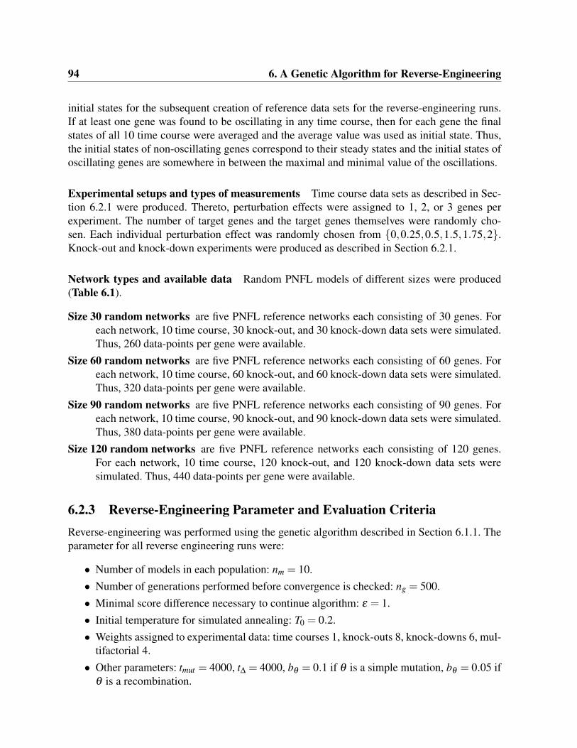
Systems biology as a field of research is concerned with studying of biological systems as awhole to understand their structure and dynamics ([1] p. 315, [2, 3, 4, 5, 6]). The parts of bio-logical systems have been revealed to a great extent by various “-omics”: genomics, proteomics,metabolomics, transcriptomics, etc ([7] with various links to data repositories). High-throughputtechnologies like micro-arrays [8, 9, 10], next-generation sequencing [11, 12, 13], and mass spec-trometry [14, 15, 16, 17, 18] have been used to collect comprehensive data sets. Now, systemsbiology aims to infer the molecular networks and mechanisms that connect these parts and causethe phenotypic properties of biological systems [19].

One of the central questions of systems biology is how the complex dynamical behaviorof a system emerges from individual interactions between biological molecules. Although thisbehavior emerges from their interplay, it is not predictable by studying the properties of singlemolecules or processes alone ([1] p. 310, [20, 21]). To study the dynamic behavior of a system,one has to investigate the dynamic interplay of molecules. This interplay can be studied in silicousing computational models of the system.

1.1 Models of Biological SystemsModels of biological systems represent aspects of natural phenomena in a simplified way. Thevalue of such models is determined by their usefulness to explain empirical observations in a waythat makes predictions possible ([22] p. 90). Such predictions must allow verification or falsifi-cation by empirical observations ([22] p. 244). Every biological system - an organism, a cell, acellular compartment, a signal transduction pathway, a part of a pathway - is constituted of enti-ties and interactions. A model of such a biological system is an abstract, simplified representationof this system and includes abstract, simplified representations of entities and interactions.

Entities The abstract term entity may refer to any kind of species, actor, subject, or part of abiological system, as well as to all kinds of aggregations of these. Thus, the term entity mightrefer to a single, specific biological molecule, for example a specific transcription factor Ai whichcurrently binds to a certain stretch of DNA in contrast to the other transcriptions factors of the sa-

4 1. Introduction

me species A1,A2, . . . ,An which are also denoted as individual entities. But the term entity mightalso refer to the whole set of transcription factors of the same kind A, which is an aggregation ofthe individual molecules. Biological molecules and sets of similar biological molecules can beseen as entities, but likewise can be parts of molecules like a gene as a part of the chromosomalmolecule or aggregations of diverse molecules, like a cell as the aggregation of its various diffe-rent constituting parts. Not only biological molecules or aggregates of these can be entities of abiological system, but also any other factors like for example the environmental conditions canbe seen as an entity of a system as well.

At any given time, a biological system is in a certain state. The current state of a system isdefined by the current states of the entirety of entities that are part of the system. In turn, thecurrent state of an entity is defined by its current state with respect to properties of this entity.Each entity possesses a variety of properties that describe it. For example, a protein has a mass,a shape, a location within the cell. The set of proteins of a specific species has a concentration inmol or the proportion of phosphorylated proteins as a property. A gene has an expression level,which in fact describes the amount of the according mRNA, but nevertheless can be seen as aproperty of the gene. A cell has a type, e.g. blood or liver cell, and is in some phase of the cellcycle. The cellular environment has a temperature, a pH-level, etc. The current state of an entitywith respect to a property can be specified by a numerical or linguistic value. Thus, the currentstate of an entity is defined by the collection of numerical/linguistic values of all its properties.

Interactions Entities in a biological system interact. Kinases phosphorylate other proteins orthemselves, transcription factors regulate genes, mRNA is degraded, small molecules diffuse(both can be seen as a self-interactions or interactions with the environment), the environmentalconditions influence enzymatic reactions, etc. In short, all kinds of (cellular) processes can beseen as interactions between pairs of entities or between sets of entities. Interactions betweenentities cause the dynamics of a biological system. Without them, the system would be static.

In general, a set of entities affects another set of entities via an interaction. The entities of thefirst set can be denoted effectors, those of the latter set targets. The same entity can be present inboth sets. It can be effector and target at the same time. Through the interaction of effectors andtargets, the state of the targets is changed depending on the current state of the effectors. Thisstate change typically affects only a subset of the properties of the targets and is influenced onlyby the current states of a subset of properties of the effectors.

System Dynamics Entities and interactions primarily provide a static description of a system.They define relevant actors, their connectivity, possible paths of effect propagation, etc. If tem-poral and spatial dimensions are additionally considered, the dynamics of a system emerge fromthe interactions of entities. The current state of a system is defined by the states of its entities.Interactions like regulation of expression, enzymatic conversion, or transport processes causestate changes. A system’s dynamics can be seen as trajectories of these state changes in time andspace.

These dynamics are complex and can not be directly derived from a static description. Espe-cially feedbacks cause a high degree of complexity. They can provide robustness and stability,

1.1 Models of Biological Systems 5

cause oscillations, or enhance, damp, or shutdown signal flow. Such a complex behavior can on-ly be uncovered by studying the dynamics of a system. Thus, such a study is essential to gaininsights into a system’s properties and to allow predictions about its reaction to perturbations.

1.1.1 Abstraction and Representation

Every model of a biological system includes abstract representations of entities and interactions.Entities are represented by a selection of their properties and the associated values. Thus, a mo-del includes a representation of the state of each entity with respect to some but typically notall properties. Most often, each entity is represented by a single state only, e.g. its concentrati-on, expression level, or fold change. In computational models, states are typically representedas numerical values. The abstractions of interactions represent the effector-target relationshipsbetween entities. Most often, they also define quantitatively how the states of effector entitiesaffect the states of target entities. In computational models, interactions are typically representedby mathematical functions.

Irrespective of the actual applied modeling technique (Section 1.2), all models can be gra-phically represented as networks of nodes and edges. As we consider biological systems as col-lections of entities and interactions, any biological system is inherently structured as a network,and likewise is implicitly or explicitly any model of such a system. How a network is actuallyderived from a model depends on the modeling technique and the desired type of network. Forexample, nodes could correspond to entities and edges to interactions, or both entities as well asinteractions are nodes, e.g. as realized in Petri nets.

In general, only those states of entities and those interactions are included in a model that areof interest for the creator of the model. I.e. a model is built with a purpose and ideally includesexactly those entities and interactions that serve this purpose. Models are used for:

• Visualization of current knowledge in terms of entities and interactions that are relevantfor a system.

• Structural analysis of the network, e.g. connectivity, degrees, clustering, or cycles.

• Analysis of a system’s behavior given different initial states, parametrizations of functions,perturbations during execution, etc.

• Tests of hypotheses about the system by comparison to (new) experimental data

One can distinguish two basic types of models: static models and executable or dynamic mo-dels ([23] p. 10). A static model is equivalent to a graphical representation of entities and theirinteractions, for example as a network. It gives an idea about the connectivity of the underlyingnetwork and might as well provide basic information about the type of effector-target relati-onships, e.g. whether an effector acts activating or inhibiting on a target. They do not provideenough information to allow for a calculation of state changes, i.e. to predict future states basedon the current states. Static models are suited to visualize or represent our knowledge of a system,for example as a figure in scientific literature. They can be very well suited to perform structuralanalysis of the model’s underlying network.

6 1. Introduction

Dynamic models are more complex models. They have to provide enough information toallow for the simulation of a system. States and interactions have to be defined such that givensome initial states one has to be able to calculate state changes and thus future states. In dynamicmodels, interactions are represented as functions that can be evaluated based on the current statesof effectors to calculate the state changes for their targets. These models can be used to learn howthe observed behavior of a system arises, and can be used for in silico studies of the effects ofperturbations. As dynamic models can be easily converted to static models without additionalinformation, they can be used for anything that static models can be used for.

Models are built based on current knowledge and hypotheses about a system’s entities and in-teractions. Hereby, the term knowledge denotes all kinds of available information, which can beroughly divided into two categories. First, experimental data, i.e. empirical observations of statesand interactions during various experiments. Second, prior knowledge, i.e. knowledge about en-tities and interactions that can be obtained from scientific literature or other readily availablesources. Examples for experimental data are concentration or expression levels of moleculesat certain time points during experiments, binding affinities of molecules, conversion rates, etc.Prior knowledge might include reaction rates, the role of entities for example as transcription fac-tors, knowledge about the chemical composition of a medium, etc. Models are built manually byan expert or user, by applying an automated or supervised reverse-engineering procedure, or by acombination of these. Model creation is usually done within a mine-model-mine cycle ([20],[23]pp. 17,[24, 25]):

• knowledge about a system is collected and hypotheses are formulated• a model is created based on the knowledge and hypotheses• new knowledge is collected and the model is compared to this knowledge• hypotheses are modified and a new model is created, etc.

A good or adequate model of a biological system matches currently available prior knowledgeand reproduces currently available experimental observations. If a model contradicts prior know-ledge or data, this contradiction has to be justified. For example, if the network structure of themodel contradicts prior knowledge but the simulated data matches experimental data, then onecan conclude that the current knowledge about network structure is inaccurate and should bemodified. Thus, the observed contradiction is justified by the explanation of experimental dataand results in the modification of the current hypothesis about network structure.

1.1.2 Reverse-EngineeringOne of the main goals of research of biological systems is to reverse-engineer networks from ex-perimental data and to use them to investigate physiological and pathological mechanisms ([26]p. 222 , [27, 28]). Reverse-engineering is an inverse problem - it is the process of obtainingeffector-target relationships between entities based on experimental observations. Although theactual molecular mechanisms of effector-target relations are hardly measurable, their effects canbe observed in large-scale biochemical data. The observed effects allow conclusions about theunderlying relations between entities [29].

1.2 Computational Modeling in Bioinformatics 7

Reverse-engineering of a dynamic model corresponds to creating a candidate model andusing it to simulate data. If the simulated and experimental data are similar, the created dyna-mic model can be considered as an adequate representation of the true biological system, thereference system. Such reverse-engineered models are only approximations of the reference sy-stem, as the created models will be simplifications of the reference: relevant entities might bemissing and the applied functions might be insufficiently complex. As measurements are typi-cally incomplete, erroneous, and noisy, even a perfect model of the system might not be able toreproduce the experimental data perfectly.

The number of data-points necessary for reverse-engineering depends on the complexity ofthe (computational) modeling technique that is used for inference, the number of effectors thatact on each target, the measurement error and signal-to-noise ratio, etc [27]. Very simple modelsthat only represent functional associations between entities without defining any dynamics, i.e.static models, require the least amount of data. For example, pairwise correlation based clusteringapproaches require about log(n) measurements of all n entities [30]. More involved approachesthat allow a dynamic simulation of processes but still are significant simplifications of a systemalready require a number of measurements that grows exponentially with the number of invol-ved entities. For example, 2n measurements of n genes are necessary to obtain all functions ofBoolean models, or about 2K if the number of effectors is restricted to K [30]. Models that in-clude continuous representations of states and allow for non-linear effects require even higheramounts of data than do linear or Boolean models, and typically the number of required mea-surements surpasses the number of those available [28, 29]. Functional relationships betweeneffectors and targets can only be successfully assessed if the effector-induced changes in thetarget’s states surpass the experimental and measurement noise (signal-to-noise ratio) [27]. Allcommon high-throughput technologies suffer from noise: micro-array measurements are influ-enced by hybridization effects or dye-related signal correlation bias, next-generation-sequencingis influenced by unspecific sequence alignments and PCR bias, mass spectrometry is impairedby a lack of detection sensitivity and data reproducibility [31, 32, 33, 34, 35].

1.2 Computational Modeling in BioinformaticsA wide variety of computational techniques has already been applied for modeling of biologi-cal systems. These techniques differ in their level of detail, their representation of entities andinteractions, their graphical representation of the system, and allow for different types of analy-sis. The choice of a computational technique depends on the purpose of model building and theavailability of biological knowledge [36, 37, 38].

Static models are used to represent the topology of a biological system, i.e. the networkstructure that emerges from entities and their interactions, and have for example been derivedbased on DNA-binding motifs [39, 40, 41], co-expression clustering [42, 43, 44, 45, 46], pair-wise correlation, mutual information, or other correlation coefficients [47, 48, 49, 50, 51], nestedeffects [52, 53], or Bayesian inference [54, 55, 56].

Dynamic models are representations of a system that allow for the inference of dependentvariables as functions of independent variables, where these variables are representations of states

8 1. Introduction

of entities [27]. Thereby, these models can be used to predict the behavior of a system at futuretime points starting from an initial state that is derived from empirical data [27, 29]. In fact, theability of a computational model to generate experimentally testable hypotheses is a major qualitycriterion. Dynamic modeling techniques have been extensively reviewed [57, 58, 59, 60, 61,62, 63]. Some of the most common modeling techniques are based on Boolean or multi-valuedlogic [64, 65, 66, 67, 68, 69, 70], Petri nets [71, 72, 73, 74], or differential equations [75, 61, 76,77, 78, 79]. Dynamic computational models have been widely used to study biological systems,for example apoptosis pathways [80, 81, 82], yeast cell cyclce [83, 84, 85, 86], mammalian cellcycle [87, 88, 89], mouse and drosophila embryonic pattern formation [90, 91, 92, 93], C. elegansand A. thaliana development [94, 95, 96, 97, 98], or biosynthesis of metabolites [99, 100, 101].

In the following, two techniques will be shortly discussed as they are relevant to this work:discrete logic models and models based on ordinary differential equations (ODE models).

1.2.1 Discrete Logic Models

Discrete logic models are radical simplifications of biological systems. In such models, it isassumed that entities can be described as being in two or more discrete states with respect toa property. If all entities are in one of two states, e.g. on or o f f , 1 or 0, present or absent,then discrete logic models are typically referred to as Boolean models, whereas if entities canbe in one of three or more states, discrete logic models can be referred to as multi-valued logicmodels. The domain of discourse of any property is discretized using strict borders according tothe number of desired states. For example, the domain of discourse of all concentrations, R≥0,can be discretized based on a threshold concentration c, such that all concentrations that aregreater than c are described as on while all concentrations lower or equal than c are o f f . Hereby,on and o f f can be seen as sets, and all possible concentration values are assigned to either ofthem. If an entity is described as being in state on with respect to its concentration, then thismeans that the entity’s concentration is greater than c and in the set on. A specific threshold, e.g.c = 10 mol, has to be chosen only if empirical data has to be discretized, e.g. to be compared toa model’s predictions, or to be used to assign initial states. If a model is purely theoretical, suchspecific thresholds are only implicitly assumed. A discretization can be based on various aspects,but the most important are:

• Experimentally observed, typical abundances. If several typical value ranges for the abun-dance of an entity have been observed in experiments, then a discretization might reflectthese different typical abundances. For example, an entity is either in state on (highly abun-dant) or o f f (lowly abundant), as applies for the independent variable y in Figure 1.1(left).

• Functional implications. If the concentration of an entity is in a certain value range, then ithas a certain effect to its targets, and this effect is considerably different if the concentrationis within another value range. For example, the state on of an activator implies that its targetis in state on as well, while the state o f f implies that the target is o f f , as applies for thedependent variable x in Figure 1.1(left).


stepwise

x

ycontinuous

x

y

sigmoid

x

y

Figure 1.1 Discretization issues. (Left) A discretization of states, e.g. into on and o f f , can be mea-ningful if the values of the independent variable y (target’s state) achieve clearly distinct values for mostvalues of the independent variable x (effector’s state) and if the intermediate values appear rarely. In sucha case, it is obvious how a discretization should be performed. (Center) If there is a continuous depen-dency between y and x, a discretization is not adequate and results in spurious switches of discrete statesalthough the underlying values changed only slightly. Furthermore, it is not clear how x or y should bediscretized. (Right) There are not only extreme cases, but also mixed cases. Here, a discretization mightbe meaningful, but the aforementioned issue persists.

Thus, if an entity is described by discrete states, then a unique interpretation is inherently asso-ciated with each state, i.e. an interpretation with respect to e.g. abundance or functionality. Thefuture states of entities are determined by the current states of their effectors through logicalfunctions

yt+1 = f (xt1, . . . ,x

tK)

Such logical functions correspond to rule tables that map all possible combinations of effectorstates to states of the target entity. For example, if in a Boolean model a target entity has Keffectors, then each one the 2K combinations of effector states is either mapped to on or o f f .Repeated evaluation of logical functions creates a trajectory of states. The dynamics of a systemcorrespond to the trajectories of all entities.

A discretization of an intrinsically continuous property like a concentration is meaningful,if the concentration of an entity is actually found to be in few, distinct value ranges, and if theconcentration switches between these value ranges so fast that intermediate concentrations valuesare rarely found or have no significant biological meaning. For example, a transcription factorcould be found to be either expressed or not depending on the observed cell type [28]. Thistranscription factor could exhibit a switch-like, non-linear dependency on its effectors. Patternsof expressed and non-expressed transcription factors then specify cell types. These pattern mayswitch during differentiation, and such behavior can be successfully modeled by discrete logicmodels [30].

A major drawback of discrete logic models is that they can not represent intermediate statesand thus they are not suited to model small or slow state changes and easily generate spuriousresults [28, 61]. For example, the concentration of a metabolite increases cumulatively as longas an according producing reaction occurs that converts an educt to the metabolite. If during thisprocess, the metabolite’s concentration exceeds the threshold c, the discretization switches imme-diately from o f f to on although the actual concentration changed only marginally (Figure 1.1).

10 1. Introduction

1.2.2 Ordinary Differential Equations ModelsOrdinary differential equations (ODE) models allow for a complex representation of systems.The states of entities are represented as continuous, real-valued variables, thus allowing for arbi-trary small state changes. State changes during infinitesimal time intervals are defined by linearor non-linear differential equations.

yt+dt = yt +dydt

,dydt

= f (xt1, . . . ,x

tK)

Thus, the new state of an entity is defined by summation of its current state and the state change.The effective state changes are determined by the current states of effectors, the applied reactionrate functions, and their parametrization. Due to the flexibility in the composition of reaction ratefunctions and their parametrization, complex dependencies of effector and target entities can berealized in ODE models.

saturating

x

dy/d

t

linear

x

dy/d

t

accelerating

x

dy/d

t

Figure 1.2 Obscured functionality. All three curves were created using the Hill equation with x∈ [0,1],c = 1, and k = 3. In all three cases, x has an increasing effect to dy/dt, but these effects are qualitativedifferent. (Left) With parameter n = 0.3, the effect is saturating at high x. (Center) With n = 1, the effectis continuously increasing. (Right) With n = 5, the effect is accelerating with increasing x. This differentqualitative behavior is not obvious from the equation alone, especially for users without an extendedmathematical background.

A major drawback of ODE models is that the functional dependencies between entities are noteasily interpretable, especially for users without an extended mathematical background [61]. Thefunctionality of a system strongly depends on its parametrization. It may exhibit a significantlydifferent behavior for different parametrizations, not only in a quantitative, but also in a quali-tative way. For example, a commonly used and relatively simple representation of a functionaldependency is based on the Hill equation

dydt

= c · xn

Kn + xn

Depending on the parameters K and n, the qualitative effect of x to dy/dt can be significantlydifferent, ranging from saturating to accelerating (Figure 1.2) or from continuous to stepwiseeffects (like in Figure 1.1). Thus, not even a “simple” functional dependency between a singleeffector and its target can be comprehended by an examination of the according function alone,


much less can the full model. The interpretation of the model by a user is only facilitated ifthe model’s creators explicitly provide additional information, or if the user performs additionalanalysis, for example by creating figures that display functional dependencies.

Analogously, ODE models do not offer an inherent interpretation of states. The continuousvariables can achieve arbitrary values that do not stand out in any obvious aspects. An inter-pretation occurs not until the ODE model is additionally illustrated or is augmented by furtheranalysis. For example, the different functional implications of the value ranges of independentvariable x in Figure 1.2 (right) only become apparent through investigating and explicitly visua-lizing its effect to dy/dt.

signal

product

cofactor

activate product

actiavate cofactor short signal burstslow signal decaypermanent signal

signal moleculecofactor molecule product molecule

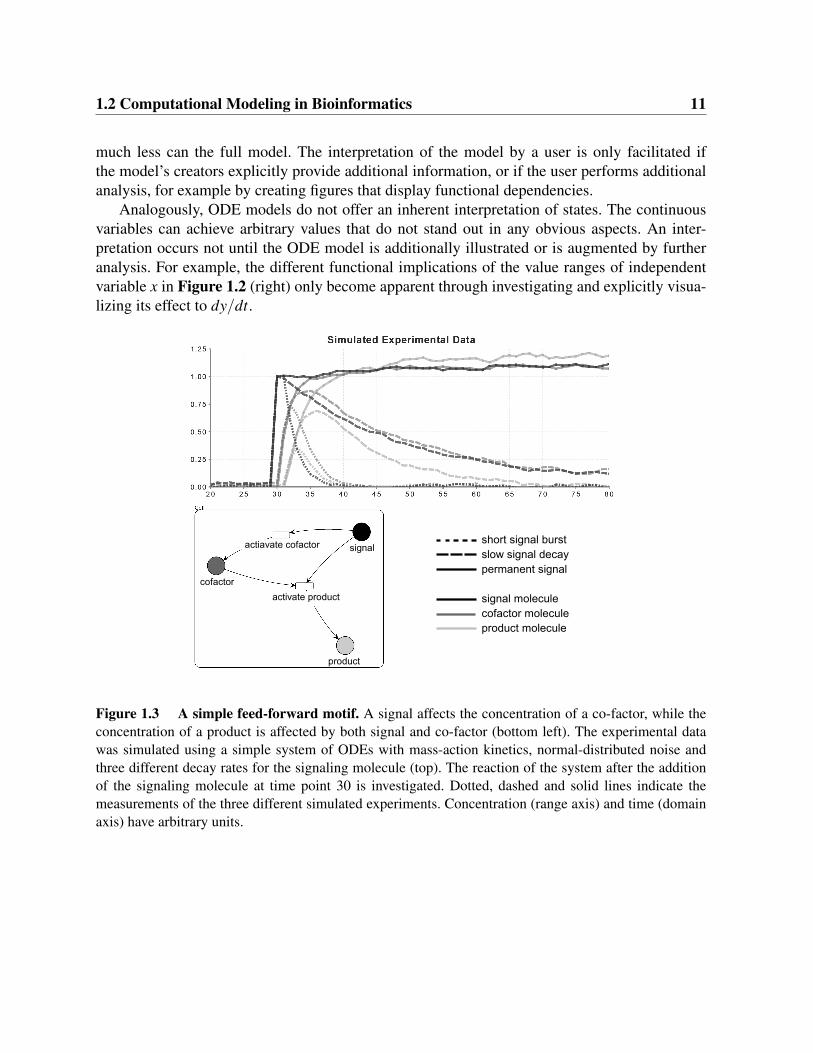
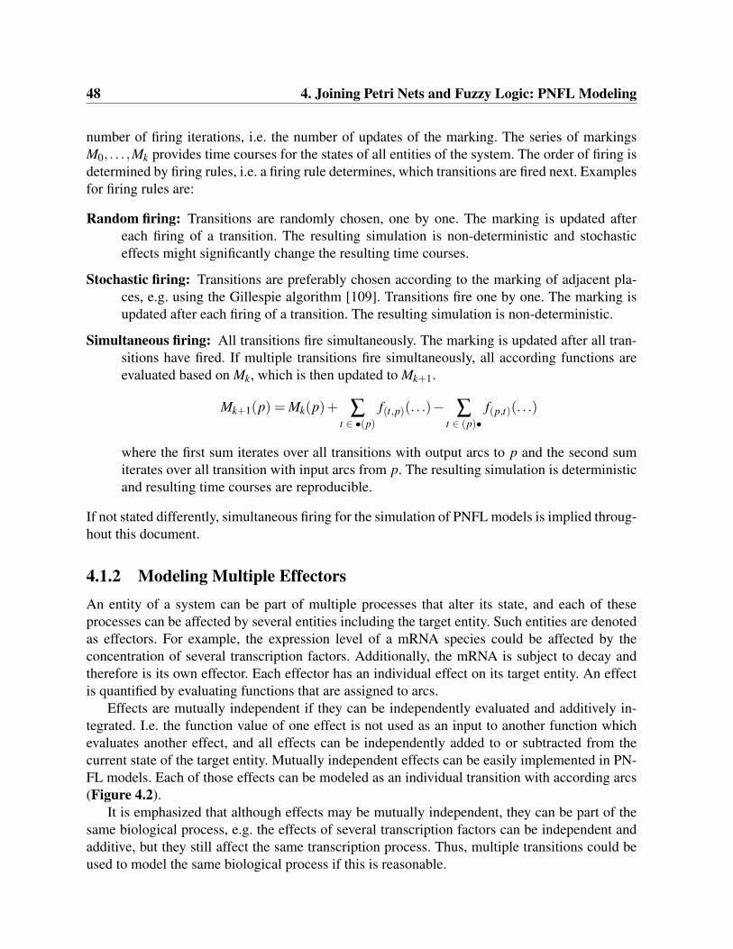
Figure 1.3 A simple feed-forward motif. A signal affects the concentration of a co-factor, while theconcentration of a product is affected by both signal and co-factor (bottom left). The experimental datawas simulated using a simple system of ODEs with mass-action kinetics, normal-distributed noise andthree different decay rates for the signaling molecule (top). The reaction of the system after the additionof the signaling molecule at time point 30 is investigated. Dotted, dashed and solid lines indicate themeasurements of the three different simulated experiments. Concentration (range axis) and time (domainaxis) have arbitrary units.

12 1. Introduction

1.3 Qualitative KnowledgeKnowledge about biological entities and of most kinds of biological data is typically incompleteand imprecise. This is caused by the size and complexity of biological systems and processes(biological noise) and by the inexactness of measurements, post-processing methods, or otherkinds of technical noise [29]. So, when considering biological data, one typically works withaverage values characterized by smaller or larger variances. And most of the time, some kindof best guess (e.g. median) is considered as the truth, for example as the true concentration ofa protein. Often enough, one not even knows the correct scales of biological data or has only arough idea about the concentrations or other properties of biological entities. In addition to theuncertain data, scales and exact quantities may not even be of great importance in a biologicalsystem, for example with respect to its stability [59].

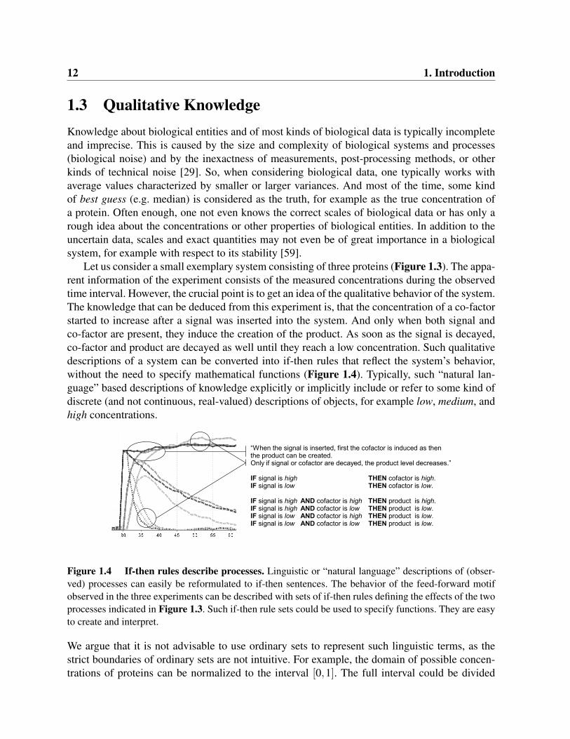
Let us consider a small exemplary system consisting of three proteins (Figure 1.3). The appa-rent information of the experiment consists of the measured concentrations during the observedtime interval. However, the crucial point is to get an idea of the qualitative behavior of the system.The knowledge that can be deduced from this experiment is, that the concentration of a co-factorstarted to increase after a signal was inserted into the system. And only when both signal andco-factor are present, they induce the creation of the product. As soon as the signal is decayed,co-factor and product are decayed as well until they reach a low concentration. Such qualitativedescriptions of a system can be converted into if-then rules that reflect the system’s behavior,without the need to specify mathematical functions (Figure 1.4). Typically, such “natural lan-guage” based descriptions of knowledge explicitly or implicitly include or refer to some kind ofdiscrete (and not continuous, real-valued) descriptions of objects, for example low, medium, andhigh concentrations.

“When the signal is inserted, first the cofactor is induced as then the product can be created.Only if signal or cofactor are decayed, the product level decreases.”

IF signal is high THEN cofactor is high.IF signal is low THEN cofactor is low.

IF signal is high AND cofactor is high THEN product is high.IF signal is high AND cofactor is low THEN product is low.IF signal is low AND cofactor is high THEN product is low.IF signal is low AND cofactor is low THEN product is low.

Figure 1.4 If-then rules describe processes. Linguistic or “natural language” descriptions of (obser-ved) processes can easily be reformulated to if-then sentences. The behavior of the feed-forward motifobserved in the three experiments can be described with sets of if-then rules defining the effects of the twoprocesses indicated in Figure 1.3. Such if-then rule sets could be used to specify functions. They are easyto create and interpret.

We argue that it is not advisable to use ordinary sets to represent such linguistic terms, as thestrict boundaries of ordinary sets are not intuitive. For example, the domain of possible concen-trations of proteins can be normalized to the interval [0,1]. The full interval could be divided

1.4 Our Contribution 13

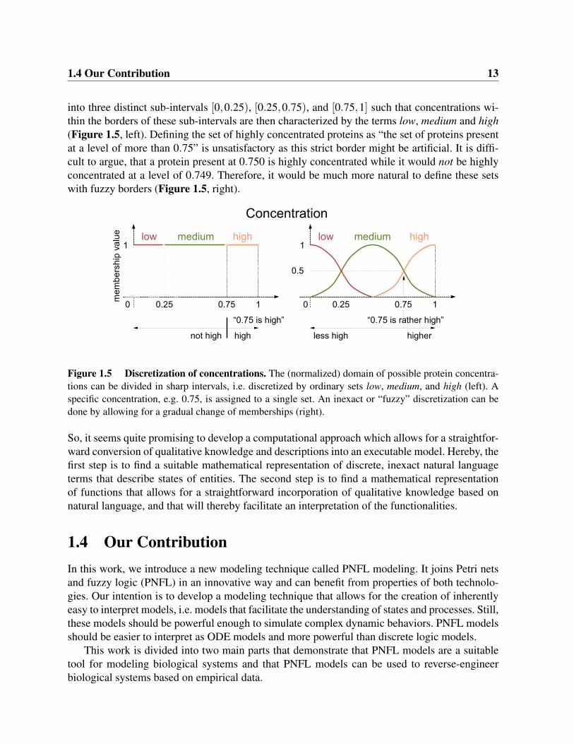
into three distinct sub-intervals [0,0.25), [0.25,0.75), and [0.75,1] such that concentrations wi-thin the borders of these sub-intervals are then characterized by the terms low, medium and high(Figure 1.5, left). Defining the set of highly concentrated proteins as “the set of proteins presentat a level of more than 0.75” is unsatisfactory as this strict border might be artificial. It is diffi-cult to argue, that a protein present at 0.750 is highly concentrated while it would not be highlyconcentrated at a level of 0.749. Therefore, it would be much more natural to define these setswith fuzzy borders (Figure 1.5, right).

Concentration

medium highlow

0.25 10 0.75

1

“0.75 is rather high”

medium highlow

0.25 10 0.75

1

less high higher

0.5

“0.75 is high”

not high high

me

mb

ers

hip

va

lue

Figure 1.5 Discretization of concentrations. The (normalized) domain of possible protein concentra-tions can be divided in sharp intervals, i.e. discretized by ordinary sets low, medium, and high (left). Aspecific concentration, e.g. 0.75, is assigned to a single set. An inexact or “fuzzy” discretization can bedone by allowing for a gradual change of memberships (right).

So, it seems quite promising to develop a computational approach which allows for a straightfor-ward conversion of qualitative knowledge and descriptions into an executable model. Hereby, thefirst step is to find a suitable mathematical representation of discrete, inexact natural languageterms that describe states of entities. The second step is to find a mathematical representationof functions that allows for a straightforward incorporation of qualitative knowledge based onnatural language, and that will thereby facilitate an interpretation of the functionalities.

1.4 Our ContributionIn this work, we introduce a new modeling technique called PNFL modeling. It joins Petri netsand fuzzy logic (PNFL) in an innovative way and can benefit from properties of both technolo-gies. Our intention is to develop a modeling technique that allows for the creation of inherentlyeasy to interpret models, i.e. models that facilitate the understanding of states and processes. Still,these models should be powerful enough to simulate complex dynamic behaviors. PNFL modelsshould be easier to interpret as ODE models and more powerful than discrete logic models.

This work is divided into two main parts that demonstrate that PNFL models are a suitabletool for modeling biological systems and that PNFL models can be used to reverse-engineerbiological systems based on empirical data.

14 1. Introduction

In part one, the Petri net and fuzzy logic modeling technique is introduced and defined andit is shown that PNFL is suited to model and analyze the behavior of biological systems. Here-by, the PNFL technique is stepwise introduced in the four main sections of part one. Section 2describes how states of biological entities are represented using fuzzy sets (published in [102]).The use of fuzzy sets is illustrated by representing concentrations, fold-changes, and expressionvalues. Section 3 describes how the functionalities of interactions are represented as fuzzy logicsystems (published in [102]). It is shown how fuzzy logic systems can be designed such that theymimic commonly used functionalities like mass-action kinetics, Hill-functions, and logic gates.Section 4 defines PNFL models and shows how they can be used to model and analyze biologi-cal systems (published in [103]). Section 5 applies PNFL to model a prokaryotic transcription-translation system (published in [104]). A PNFL model is compared to an ODE model of thesame system and it is shown how these models can be utilized to make predictions that allow forhypotheses testing.

In part two, we demonstrate how PNFL models can be reverse-engineered from empiricaldata. Therefore, we describe a non-deterministic genetic algorithm that can successfully reverse-engineer small PNFL models (Section 6, published in [105]). In addition, we present methodsthat improve prediction results for larger networks (Section 7) and post-process the predictionsof non-deterministic reverse-engineering algorithms (Section 8).

To facilitate readability, we include basic definitions of fuzzy sets, fuzzy logic systems, etcwithin the sections of part one. An in-depth theoretical background about fuzzy logic and appro-ximate reasoning is provided in the appendix (Section A).

Part I

Modeling with Petri Nets and Fuzzy Logic

Chapter 2

Fuzzy Sets Describe States of BiologicalEntities

At every point in time, biological entities like proteins, RNAs, cells, etc are in specific states withrespect to certain properties. For example, such properties could be the concentrations of proteinsin cells or compartments, fold-changes of mRNA species between different conditions, relativeabundances of transcript isoforms, or the current phase of the cell cycle. To some extent, theseproperties can be measured or assessed in experiments. This gives us quantitative or qualitativeinformation about the the current state of an entity. Of course, this information is often inaccurateor erroneous. Examples for obtained information:

1. Fluorescence measurements of proteins provide intensity levels, which might be convertedinto estimates of molar concentrations. This gives us absolute quantitative informationabout the proteins’ concentrations at a certain time point, i.e. their concentration states.

2. RNA-seq or micro-array measurements of a transcriptome provide mRNA expression orintensity levels, which might be converted into fold-changes with respect to expressi-on/intensity levels obtained from a reference experiment. This gives us relative quantitativeinformation about the change of mRNA expression, i.e. the fold-change states of mRNAs.

3. Visual assessment of cells provides information about their phenotypes, i.e. whether thesecells exhibit a certain phenotype or not. This gives us qualitative information about thesecells, i.e. their phenotypic state.

All observations and the derived states have a domain of discourse D, i.e. their values are ta-ken from a defined range or set of possible values. We denote values x ∈ D as crisp values, incontrast to fuzzy values as introduced below. The domain of discourse depends on the type ofobserved property, the type of measurements or assessments, and the type of post-processing ofthe observed data. For example:

1. Concentrations might be in R≥0 in combination with a unit like mol, or might be relative,unit-less abundances in [0,1].

2. Expression changes might be log-fold-changes in R.

18 2. Fuzzy Sets Describe States of Biological Entities

3. Cell phenotypes might be taken from a discrete, finite categories set, e.g. cell cycle phases{G0,G1,S,G2,M}.

Computational models of biological systems have to represent the current states of biologicalentities. Based on these representations, a system’s behavior can be predicted or investigated(Section 1.1).

100 %

0 %

45 %

time <0.74,0.26,0.0>

80 %

13 %

<0.1,0.9,0.0> <0.0,0.4,0.6>

low

, med

ium

, an

d h

igh

re

lati

ve c

on

cen

trat

ion

s

Timecourse Measurements

fuzzification of relative concentrations

1

100 % 0 %

0

low high medium

Concentrations

<0.74,0.26,0.0> <0.1,0.9,0.0>

<0.0,0.4,0.6>

45 % 80 % 13 % mem

ber

ship

val

ue

fuzzification of relative concentrations

Figure 2.1 Fuzzy sets describe states. Assume that some measurements of protein concentration du-ring an unspecified time interval are given (left panel). We quantify protein concentration as relative ab-undance. The domain of discourse comprises all real numbers in [0,100] (unit %). The interval [0,100]can be fuzzy discretized using three fuzzy sets that represent states of low (µlow), medium (µmedium), andhigh (µhigh) concentrations (right panel). The fuzzy sets map relative concentrations (x-axis) to member-ship values (y-axis). This three fuzzy sets constitute a fuzzy concept, and fuzzification of concentrationx ∈ [0,100] results in a fuzzy value < µlow(x),µmedium(x),µhigh(x) >. This fuzzy value represents thecurrent state of an entity with respect to a property (e.g. concentration) that in turn is described by theaccording fuzzy concept.

The representation of states with respect to certain properties can be based on fuzzy sets (Sec-tion A.2, [106]). They refer to aspects of the underlying biological property, e.g. “low concen-trations”, “medium concentrations”, or “high concentrations”, an can be interpreted as a fuzzydiscretization of the according domain of discourse D. A fuzzy set µ maps all states x ∈D to theinterval [0,1], i.e. it assigns a membership value to each x that defines the degree of membershipof x to the fuzzy set:

µ : D→ [0,1]

The process of mapping a crisp value to a membership value is called fuzzification (Section A.2).If a state has a high degree of membership to a fuzzy set (high membership value) then theaccording aspect of the biological property applies to this state to a high degree. For example,fuzzy sets describing low concentrations assign high membership values to small x∈D and smallmembership values to large x ∈ D (Figure 2.1). Thus, a single fuzzy set provides a membershipvalue that represents a state with respect to single aspect of a biological property.

19

To describe a state with respect to several properties, several fuzzy sets that have the sa-me domain of discourse can be combined. Such combinations - called fuzzy concepts - can berepresented as tuples < µ1, . . . ,µn >. Such a fuzzy concept is a collection of fuzzy sets that de-scribe the state of a biological entity with respect to the same property, e.g. concentration orfold-change. Fuzzyfication of a crisp value x ∈ D by the fuzzy sets of a fuzzy concept gives usa vector < µ1(x), . . . ,µn(x) > with entries µi(x) ∈ [0,1]. This vector is the actual representationof the state with respect to the fuzzy concept. This vector is called fuzzy value. Fuzzy values areused as inputs for fuzzy logic systems (Section 3). State changes and thus a systems behavioris computed based on the fuzzy value representation. The unified description of continuous aswell as discrete properties, like concentrations and phenotypic states, by fuzzy values allows fora combination of such properties in fuzzy logic systems.

The number and shape of fuzzy sets that are joined to a fuzzy concept can be freely chosenaccording to design needs, e.g. depending on the type of biological property, available expe-rimental data, or desired level of abstraction (Section 2.2). No matter how a fuzzy concept isdesigned, a fuzzy value < µ1(x), . . . ,µn(x) > derived by fuzzification of a crisp value x ∈ D hasthe following properties:

1. ∀i ∈ {1, . . . ,n} : µi(x) ∈ [0,1]2. ∑

ni=1 µi(x) ∈ [0,n]

Where property 1 corresponds to the definition of fuzzy sets and property 2 is derived fromproperty 1 and the definition of fuzzy values. Fuzzy sets that constitute a fuzzy concept mayoverlap arbitrarily and a crisp value could have a high degree of membership to several fuzzysets. However, we advise that fuzzy concepts should be designed such that ∑

ni=1 µi(x) = 1 holds.

On the one hand side, this guarantees that the domain of discourse is covered by fuzzy sets whichis important for the use of the fuzzy concept in fuzzy logic systems (Section 3). On the other hand,this follows a quite natural and intuitive interpretation of a fuzzy value. This interpretation is thata biological entity has to be in some state, thus the fuzzy value has to be non-zero, and that the“membership potential” of a state is shared out to one or several fuzzy sets, thus the fuzzy valueshould sum to one.

A straightforward way to cover the full domain of discourse with fuzzy sets is to use unboun-ded fuzzy sets, i.e. fuzzy sets that assign a membership value of 1 to all crisp values larger (orsmaller) than a given threshold (Section 2.1.4). Using triangle- or trapezoid-like fuzzy sets asdefined in Section 2.1 to constitute a fuzzy concept ensures that the induced fuzzy values alwayssum to exactly one.

Each fuzzy value < µ1(x), . . . ,µn(x) > can be mapped to a crisp value y ∈D. This process isdenoted defuzzification. In general, defuzzification derives a “most typical” crisp representativeof a given fuzzy value. A common, intuitive, and computational simple defuzzification approachis height defuzzification (Section A.3.3). Here, the crisp value y is obtained by calculating aweighted average of typical representatives of those fuzzy sets that constitute the respective fuzzyconcept:

y =∑

nj=1 y j ·µ j(x)

∑nj=1 µ j(x)


where y j is the center of gravity of fuzzy set µ j and used as its typical representative. Dependingon the design of the fuzzy concept, the original crisp value x and the defuzzified value y can beidentical. This is discussed in the following section, where we introduce some common shapesof fuzzy sets and according fuzzy concepts. These “most typical” crisp representatives can bestraightforwardly used for visualization and are used to store the current state of an entity inPNFL models (Section 4).

2.1 Common Shapes of Fuzzy SetsAny function µ : D→ [0,1] is a fuzzy set over the domain of discourse D. But for the applicationin modeling of biological systems, some basic shapes of fuzzy sets are especially suited. We willdiscuss triangle-, trapezoid-, and Gaussian-like fuzzy sets with the real numbers R as domainof discourse (Figure 2.2). Most often, e.g. when considering concentrations, expression levels,or fold-changes, the domain of discourse is naturally R or a subset thereof. Other domains ofdiscourse of states of biological entities can generally be mapped to the domain of real numbersR, e.g. numerical values 1,2,3, . . . can be used to represent purely qualitative states like cell phe-notypes. Further, we will discuss unbounded fuzzy sets, i.e. fuzzy sets that assign a membershipvalue of 1 to all x ∈ D that are larger or smaller than defined thresholds. Such fuzzy sets areespecially suited to ensure that the domain of discourse is fully covered by a fuzzy concept.

2.1.1 Triangle-like Fuzzy SetsThe membership function of a triangle-like fuzzy set is defined as (Figure 2.2A):

µtri(x) =

0 if x≤ lx−l

mp−l ·m if l < x < mp

m if x = mpr−x

r−mp ·m if mp < x < r

0 if r ≤ x

Parameter m ∈ [0,1] specifies the maximum of µ tri and is typically 1. Parameters l,r,mp ∈ R(left border, right border, maximum point) specify the shape and location of the triangle-likefuzzy set with respect to the domain of discourse. Defuzzification is usually performed usingthe center of gravity of the triangle-like fuzzy set. This corresponds to mp if the triangle isisosceles, i.e. if mp− l = r−mp. We advise to use mp as pseudo center of gravity also for non-isosceles triangular shapes, as this facilitates interpretation of defuzzified values. It is obviousthat l ≤ x,y ≤ r ∧ |x−mp| 6= |y−mp| ⇔ µ tri(x) 6= µ tri(y) holds for triangle-like fuzzy sets.Thus, the membership value of a state x is sensitive to changes in x as long as the fuzzy setcovers x, i.e. if x is between l and r. From a functional perspective, using triangle-like fuzzy setsresults in systems that are sensitive to state changes, i.e. small variations in states of effectorscan be propagated to their targets. Furthermore, using triangle-like fuzzy sets is advantageous ifa one-to-one mapping of a crisp value to its fuzzy value is desired.

2.1 Common Shapes of Fuzzy Sets 21

A) Triangle-like fuzzy set

domain of discourse

Triangle-like fuzzy concept

B) Trapezoid-like fuzzy set

1

0

mem

ber

ship

val

ue

domain of discourse

CoG

r l

a b c

mp r mp l

Trapezoid-like fuzzy concept

C) Gaussian-like fuzzy set

1

0

mem

ber

ship

val

ue

CoG

mp domain of discourse

Gaussian-like fuzzy concept

1

0

mem

ber

ship

val

ue

CoG

mp r l

a b c

1

0

𝐹𝑆0 𝐹𝑆1 𝐹𝑆2 𝐹𝑆3 𝐹𝑆4 𝐹𝑆5

b c

1

0

𝐹𝑆0 𝐹𝑆1 𝐹𝑆2 𝐹𝑆3

b c

1

0

𝐹𝑆0 𝐹𝑆1 𝐹𝑆2 𝐹𝑆3

0.5

a b

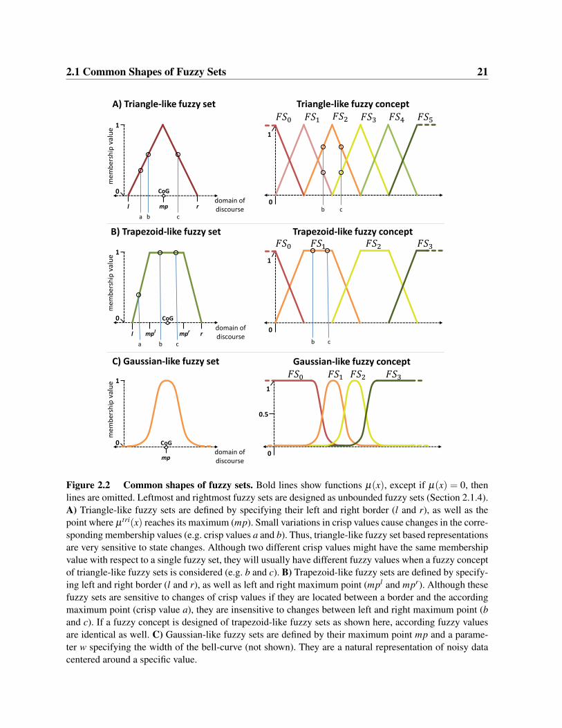
Figure 2.2 Common shapes of fuzzy sets. Bold lines show functions µ(x), except if µ(x) = 0, thenlines are omitted. Leftmost and rightmost fuzzy sets are designed as unbounded fuzzy sets (Section 2.1.4).A) Triangle-like fuzzy sets are defined by specifying their left and right border (l and r), as well as thepoint where µ tri(x) reaches its maximum (mp). Small variations in crisp values cause changes in the corre-sponding membership values (e.g. crisp values a and b). Thus, triangle-like fuzzy set based representationsare very sensitive to state changes. Although two different crisp values might have the same membershipvalue with respect to a single fuzzy set, they will usually have different fuzzy values when a fuzzy conceptof triangle-like fuzzy sets is considered (e.g. b and c). B) Trapezoid-like fuzzy sets are defined by specify-ing left and right border (l and r), as well as left and right maximum point (mpl and mpr). Although thesefuzzy sets are sensitive to changes of crisp values if they are located between a border and the accordingmaximum point (crisp value a), they are insensitive to changes between left and right maximum point (band c). If a fuzzy concept is designed of trapezoid-like fuzzy sets as shown here, according fuzzy valuesare identical as well. C) Gaussian-like fuzzy sets are defined by their maximum point mp and a parame-ter w specifying the width of the bell-curve (not shown). They are a natural representation of noisy datacentered around a specific value.


Proposition Assume a fuzzy concept consisting of n triangle-like fuzzy sets µi with increasingmaximum points mpi and left and right borders defined as follows: l1 arbitrary, r1 = mp2. ∀i,1 < i < n : li = mpi−1, ri = mpi+1. ln = mpn−1, rn arbitrary (e.g. as in Figure 2.2A). Thenfuzzification of any value x ∈ [mp1,mpn] using a fuzzy concept as defined above, and subsequentheight defuzzification with centers of gravity equal to the maximum points, results in a crispvalue y = x.

Proof Fuzzification of x ∈ [mp1,mpn] results in a fuzzy value < µ1(x), . . . ,µn(x) >. Per defini-tion, at most two entries can be non-zero. Without loss of generality, assume that these are µi(x)and µi+1(x). Thus, the defuzzified value y is defined as:

y =∑

nj=1 y j ·µ j(x)

∑nj=1 µ j(x)

=mpi ·µi(x)+mpi+1 ·µi+1(x)

µi(x)+ µi+1(x)(2.1)

As per assumption mpi ≤ x and x≤ mpi+1, Equation 2.1 can be written as:

y =mpi · ri−x

ri−mpi+mpi+1 · x−li+1

mpi+1−li+1

ri−xri−mpi

+ x−li+1mpi+1−li+1

(2.2)

Per definition of left and right borders, Equation 2.2 equals:

y =mpi · mpi+1−x

mpi+1−mpi+mpi+1 · x−mpi

mpi+1−mpimpi+1−x

mpi+1−mpi+ x−mpi

mpi+1−mpi

= mpi ·mpi+1− x

mpi+1−mpi+mpi+1 ·

x−mpi

mpi+1−mpi= x

Thus, a fuzzy concept as defined above allows a one-to-one mapping of a crisp value to its fuzzyvalue, q.e.d.

2.1.2 Trapezoid-like Fuzzy SetsThe membership function of a trapezoid-like fuzzy set is defined as (Figure 2.2B):

µtra(x) =

0 if x≤ lx−l

mpl−l ·m if l < x < mpl

m if mpl ≤ x≤ mpr

r−xr−mpr ·m if mpr < x < r

0 if r ≤ x

Parameter m∈ [0,1] specifies the maximum of µ tra and is typically 1. Parameters l,mpl,mpr,r ∈R (left border, left and right maximum point, right border) specify the shape and location ofthe trapezoid-like fuzzy set with respect to the domain of discourse. If the trapezoidal shape issymmetric, the center of gravity is at mpl + mpr−mpl

2 . As mpl < x,y < mpr ∧ x 6= y⇔ µ tra(x) =µ tra(y) holds, trapezoid-like fuzzy sets are robust against changes of x within the top base, i.e.different crisp values may have identical membership values. Trapezoid-like fuzzy sets can beused to define regions where the exact value of a state is not crucial or irrelevant for a systemsbehavior, e.g. when a model with a high level of abstraction is created.

2.1 Common Shapes of Fuzzy Sets 23

2.1.3 Gaussian-like Fuzzy SetsThe membership function of a Gaussian-like fuzzy set is defined as (Figure 2.2C):

µgau(x) = m · e−

(x−mp)2

2w2

Parameter m ∈ [0,1] specifies the maximum of µgau and is typically 1. Parameters mp,w ∈ Rspecify the maximum point and control the width of the curve and the center of gravity is atmp. Gaussian-like fuzzy sets are especially suited to represent noisy data centered around aspecific value e.g. when representing fold-changes derived from expression data. Please note that∀x ∈R : µgau(x) 6= 0. Thus, membership values of Gaussian-like fuzzy sets are always non-zero.

2.1.4 Unbounded Fuzzy Sets

1

0

mem

ber

ship

val

ue

Unbounded Fuzzy Sets

domain of discourse mp r

pseudo CoG

mp

pseudo CoG

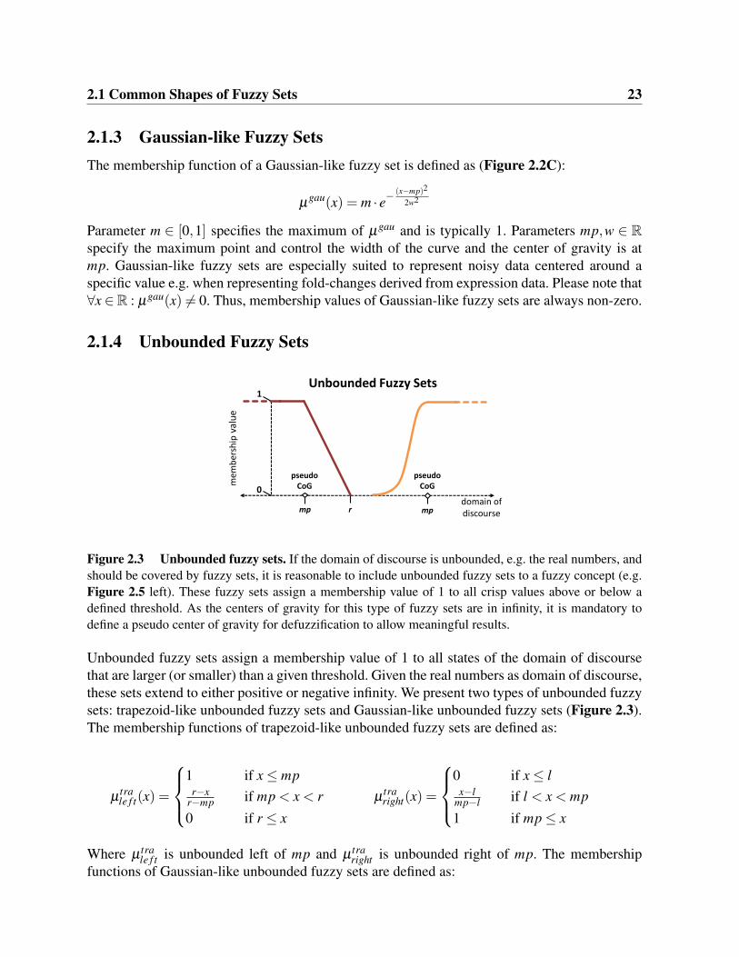
Figure 2.3 Unbounded fuzzy sets. If the domain of discourse is unbounded, e.g. the real numbers, andshould be covered by fuzzy sets, it is reasonable to include unbounded fuzzy sets to a fuzzy concept (e.g.Figure 2.5 left). These fuzzy sets assign a membership value of 1 to all crisp values above or below adefined threshold. As the centers of gravity for this type of fuzzy sets are in infinity, it is mandatory todefine a pseudo center of gravity for defuzzification to allow meaningful results.

Unbounded fuzzy sets assign a membership value of 1 to all states of the domain of discoursethat are larger (or smaller) than a given threshold. Given the real numbers as domain of discourse,these sets extend to either positive or negative infinity. We present two types of unbounded fuzzysets: trapezoid-like unbounded fuzzy sets and Gaussian-like unbounded fuzzy sets (Figure 2.3).The membership functions of trapezoid-like unbounded fuzzy sets are defined as:

µtrale f t(x) =

1 if x≤ mp

r−xr−mp if mp < x < r

0 if r ≤ x

µtraright(x) =

0 if x≤ l

x−lmp−l if l < x < mp

1 if mp≤ x

Where µ trale f t is unbounded left of mp and µ tra

right is unbounded right of mp. The membershipfunctions of Gaussian-like unbounded fuzzy sets are defined as:


µgaule f t(x) =

1 if x≤ mp

exp−(x−mp)2

2w2 if mp < xµ

gauright(x) =

exp−(x−mp)2

2w2 if x < mp1 if mp≤ x

Note that the centers of gravity of unbounded fuzzy sets are either −∞ or ∞, thus defuzzificationcan not be reasonably performed using these. We advise to use parameter mp as pseudo centerof gravity instead.

2.2 The Design of Fuzzy SetsThe number, shapes, locations, and domain of fuzzy sets must be chosen according to designneeds for a particular model or a particular set of observed data. They can be customized for eachbiological entity, e.g. concentrations of different proteins can be represented by different fuzzyconcepts. Moreover, the same property of an entity can be represented by several different fuzzyconcepts. For example, if it is an input to different fuzzy logic systems, i.e. when the biologicalentity is part of several different processes, and different representations are reasonable due tofunctional considerations. There are multiple aspects that influence the design of fuzzy sets:

Functional considerations Fuzzy concepts are used as inputs for fuzzy logic systems (Secti-on 3). The number and shapes of fuzzy sets that represent a biological property determinethe possible design and power of fuzzy logic systems. Thus, one of the most importantdesign considerations is guided by the intended functionality. For example, it is often re-asonable to design fuzzy sets such that they represent concentrations that imply a similarfunctional behavior (Figure 2.4).

Type of biological property. The fuzzy set design depends on the type of biological entity andthe type of property that should be represented. For example, when creating a fuzzy re-presentation of concentrations, one would introduce fuzzy sets describing different con-centration levels, while when creating a fuzzy representation of fold-changes, one wouldintroduce fuzzy sets describing down-regulation, wild-type, and up-regulation (Figure 2.5left).

Range of observed data. The range of actually observed data (in contrast to the domain of dis-course) guides fuzzy set design (e.g. see fuzzy set design in Section 5). For example, ifprotein concentrations between 0 and 10 nM were observed but never higher concentra-tions, then one might use several fuzzy sets to fuzzy discretize the domain [0,10], e.g. torepresent nearly absent protein, low, medium, and high protein concentration. But a singlefuzzy set covering the domain [10,∞] might be sufficient to represent exceptionally highconcentrations.

Desired level of abstraction. The more fuzzy sets are used, the more fine-grained is the fuzzydiscretization. This might be useful for interpretation and to fine-tune the quantitative be-havior of a system, but most often a qualitatively adequate functionality can be achievedwith very few fuzzy sets (e.g. see fuzzy set design in Section 4.2).

2.3 Discussion 25

inactive active intermediate

Concentrations

1

0

mem

ber

ship

val

ue

0 concentration

0

reac

tio

n r

ate

0 concentration

V max

maximal reaction rate

reactions cease

intermediate rate

figure_fuzzy_sets_design_2

Figure 2.4 Fuzzy sets designed to represent functional properties. Cooperative binding ofligands to receptors might lead to sigmoid-shaped reaction rates depending on ligand concentration.If the concentration is too low (nearly) no processes occur. The reaction rate saturates at highligand concentrations, i.e. a further increase of concentration does not increase reaction rates. Thisconcentration dependent functional behavior can be used as a guideline for fuzzy set design. If theconcentration is below or above an intermediate concentration range, the fuzzy values are close to< 1,0,0 > (inactive) and < 0,0,1 > (active). Further decrease or increase of concentration doesnot change the fuzzy value representation.

Detection limits, precision, and robustness. Measurement methods might not be able to relia-bly detect concentrations if they are too low (or too high), thus a fine-grained distinctionof these concentration levels (e.g. by several triangle-like fuzzy sets) is not meaningful anda single trapezoid-like fuzzy set could be used instead to cover a broad range. Replicatemeasurements could differ due to technical noise or biological variances. If large variationsare found, wide fuzzy sets could be used, while narrow ones can be used otherwise.

Typical values. Fuzzy sets can be designed to represent typical values of a property, for exampleexpression levels of a certain mRNA species in two cell types. One cell type might havea low expression level of this mRNA while the other has a high expression level. Theseexpression levels that are typical for a certain cell type could be modeled as Gaussian- ortrapezoid-like fuzzy sets centered at the respective expression level (Figure 2.5 right).

2.3 DiscussionA fuzzy set describes an aspect of a biological property or concept, e.g. low concentrations, medi-um concentrations, or high concentrations, and can be interpreted as part of a fuzzy discretizationof the respective domain of discourse, e.g. a discretization of all possible concentrations. We de-note a collection of fuzzy sets that describe the same property as fuzzy concept. The current stateof an entity with respect to a property is represented by a vector of membership values, a fuzzyvalue. The membership values specify to which degree the different aspects currently apply tothe state of the entity.

In the following Section 3, we will describe how fuzzy logic systems can be used to representthe interactions of a system. Fuzzy sets are used in these fuzzy logic systems to describe the


down up wildtype 1

4

0

2 0 -2 -4

4

0

2 0 -2 -4

Fold Changes

mem

ber

ship

val

ue

freq

uen

cy

log fold-changes

type A like 1

0

0

Expression Levels

mem

ber

ship

val

ue

freq

uen

cy

expression level

0

0 expression level

type B like

log fold-changes

figure_fuzzy_sets_design_1

Figure 2.5 Designing fuzzy sets. Fuzzy sets are designed according to the type of observeddata. If expression data is given as log-fold-changes, it might be reasonable to distinguish betweenwild-type expression states (assuming noise) and differentially regulated states (left panel). If sometypical values are observed in experiments, according fuzzy sets could be defined. For example,if the expression level of a mRNA species is specific for certain cell types (right panel). Fuzzyconcepts should cover the full domain of discourse. This can be achieved by defining appropriateunbounded fuzzy sets.

2.3 Discussion 27

current states of the effectors of the interactions. Hereby, the same effector may be part of severalinteractions and may be described using different fuzzy sets in each of the according fuzzy logicsystems. So the concentration of the same effector may be described using several fuzzy conceptsat the same time, each of which are used in different fuzzy logic systems. For examples, seeFigure 4.9 in Section 4.2 and Section 5.2.2.

Furthermore, the description of a state has a direct influence to the functionality of the model.By changing the definitions of fuzzy sets, the outcomes of simulations can be changed withoutchanging the rule bases of fuzzy logic systems (see Section 3). The unified description of con-tinuous as well as discrete properties like concentrations and phenotypic states by fuzzy valuesallows for a straightforward combination of such properties in fuzzy logic systems.

The presented common shapes of fuzzy sets (Section 2.1) can be used to reflect the impact ofstate changes of crisp values to a model. If small changes of a state are meaningful and shouldaffect a model, then triangle-like fuzzy sets are a suitable representation, as the derived fuzzyvalues reflect these small changes. In particular, we have shown that fuzzy concepts can be desi-gned such that there is a one-to-one correspondence of fuzzy value and crisp value representation,and thus there is no information loss by fuzzification. If small state changes of an entity have norelevant effect to a system, then this can be reflected by using trapezoid-like fuzzy sets. Suchfuzzy sets assign the same membership value to all crisp values within a certain range. Thus,they “filter” small state changes.

A comparison to ODE and discrete logic models A drawback of ODE models is that they donot offer a direct interpretation of states. ODE models represent states of entities by real-valuedvariables only (Section 1.2.2). For example, although we may know the numerical value of theconcentration of a transcription factor, we do not know whether this concentration is relativelylow or high or typical for a certain cell type, or whether at this concentration the transcriptionfactor has a considerable effect on the transcription rates of its targets or not. This informationis hidden within the ODE model and only becomes apparent if the model is simulated and theresulting data sets are interpreted. Or, such information has to be provided as additional infor-mation. In contrast, a representation based on fuzzy sets inherently includes an interpretationof the described states with respect to a biological relevant aspect, for example with respect tothe functional impact, typical values, etc (Section 2.2). As the same entity, for example a trans-cription factor, can be represented by several fuzzy concepts at the same time, one can provideinterpretation with respect to different aspects at the same time.

Discrete logic models represent states using two or more categories, e.g. on and off, or presentand absent. These categories correspond to an interpretation of the state, but the strict borders ofthese categories are unnatural and unintuitive, as was discussed in Section 1.2.1. Furthermore,the state of an entity has to be exactly in one of the allowed states. In contrast, fuzzy sets can bedesigned with arbitrary fluent transitions of one category to the next. Thus, there are no abruptchanges of the interpretation of a state and an entity can be in a meaningful intermediate state.The main advantage of using fuzzy sets to describe states is the inherently provided interpretationof these states. This significantly facilitates understanding of models while not suffering thedrawbacks of unnatural strict discretization borders.


Author’s contribution Fuzzy set are an established concept [106]. The author describes va-rious aspects of their application to represent biological data.

Chapter 3

Fuzzy Logic Systems Give Functionality toInteractions

Interactions between biological entities represent processes that influence the future state of thetarget entities based on the current state of the effector entities. Computational models mimicinteractions by functions that operate on the computational representations of states (Section 1.1).These functions map the current states of effectors (inputs) to new states or state changes oftargets (outputs). Repeated application of functions creates a trajectory of state changes whichdescribes the dynamics of a system.

Fuzzy logic systems are functions that can be used to describe such state changes. They mapinput crisp values representing states to an output crisp value:

f ls : D1× . . .×Dn→ Dy

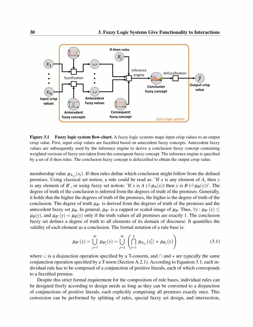
where Di is the domain of discourse of input crisp value xi and Dy is the domain of discourseof the output crisp value y. This process of mapping can be split into the intermediate steps offuzzification, fuzzy inference, and defuzzification (Figure 3.1). Fuzzification and defuzzificationof input crisp values have been described in Section 2. For each input crisp value a fuzzy conceptis used for fuzzification, denoted antecedent fuzzy concept. Fuzzy inference is specified using aset of if-then rules - the rule base - of the form:

R j : IF x1 is A j,1 AND x2 is A j,2 AND . . . AND xn j is A j,n T HEN y is B j

Where xi ∈ Di are the input crisp values, A j,i is a fuzzy set taken from fuzzy concept Ai used tofuzzify the i’th input crisp value in rule j (antecedent fuzzy set), and B j specifies the consequentfuzzy set. Consequent fuzzy sets are taken from a consequent fuzzy concept B.Each if-then rule derives a conclusion fuzzy set µB∗j : Dy→ [0,1] based on input crisp values xi andthe according consequent fuzzy set µB j . The inference of the conclusion fuzzy sets µB∗j is basedon approximate reasoning theory. We will briefly summarize the main ideas. For details, seeSection A. In approximate reasoning the (classic) truth values 0 and 1 are extended to degrees oftruth taken from the interval [0,1]. Fuzzy sets are used to quantify the degree of truth of elementsof their domain of discourse. The degree of truth of the premise ’xi is A j,i’ is identical to the

30 3. Fuzzy Logic Systems Give Functionality to Interactions

fuzzy logic system

𝑥1

fuzzification 𝑦 Output crisp

value

<,,>

<,,>

Antecedent fuzzy values

Input crisp values

𝑥𝑛

inference engine

If-then rules

𝑅𝑗

defuzzification

. . .

. . .

Antecedent fuzzy concepts

Conclusion fuzzy concept

Consequent fuzzy concept

Figure 3.1 Fuzzy logic system flow-chart. A fuzzy logic systems maps input crisp values to an outputcrisp value. First, input crisp values are fuzzified based on antecedent fuzzy concepts. Antecedent fuzzyvalues are subsequently used by the inference engine to derive a conclusion fuzzy concept containingweighted versions of fuzzy sets taken from the consequent fuzzy concept. The inference engine is specifiedby a set of if-then rules. The conclusion fuzzy concept is defuzzified to obtain the output crisp value.

membership value µA j,i(xi). If-then rules define which conclusion might follow from the definedpremises. Using classical set notion, a rule could be read as: ’If x is any element of A, then yis any element of B’, or using fuzzy set notion: ’If x is A (=µA(x)) then y is B (=µB(y))’. Thedegree of truth of the conclusion is inferred from the degrees of truth of the premises. Generally,it holds that the higher the degrees of truth of the premises, the higher is the degree of truth of theconclusion. The degree of truth µB∗ is derived from the degrees of truth of the premises and theantecedent fuzzy set µB. In general, µB∗ is a capped or scaled image of µB. Thus, ∀y : µB∗(y) ≤µB(y), and µB∗(y) = µB(y) only if the truth values of all premises are exactly 1. The conclusionfuzzy set defines a degree of truth to all elements of its domain of discourse. It quantifies thevalidity of each element as a conclusion. The formal notation of a rule base is:

µB∗(y) =m⋃

j=1

µB∗j (y) =m⋃

j=1

(n⋂

i=1

µA j,i(x′i) ? µB j(y)

)(3.1)

where ∪ is a disjunction operation specified by a T-conorm, and ∩ and ? are typically the sameconjunction operation specified by a T-norm (Section A.2.1). According to Equation 3.1, each in-dividual rule has to be composed of a conjunction of positive literals, each of which correspondsto a fuzzified premise.

Despite this strict formal requirement for the composition of rule bases, individual rules canbe designed freely according to design needs as long as they can be converted to a disjunctionof conjunctions of positive literals, each explicitly comprising all premises exactly once. Thisconversion can be performed by splitting of rules, special fuzzy set design, and intersection,

31

union, and complements of fuzzy sets as defined in Section A. In the following, we provideseveral examples of rule design and according conversions:

Negated premises A rule which contains a negative literal

R1 : IF NOT x is A T HEN y is B

can be written formally as¬µA(x) ? µB(y)

which can be converted to(1−µA)(x) ? µB(y)

which is a conjunction of positive literals. Instead of using fuzzy set µA as antecedent fuzzyset, the complement fuzzy set (1−µA) is used.

Missing premises A rule base with a rule which misses a premise

R1 : IF x1 is A1 AND x2 is A2 T HEN y is B1

R2 : IF x2 is A2 T HEN y is B2

can be written formally as

µA1(x1) ? µA1(x2) ? µB1(y) ◦ µA2(x2) ? µB2(y)

which can be converted to

µA1(x1) ? µA2(x2) ? µB1(y) ◦ µ1(x1) ? µA2(x2) ? µB2(y)

with µ1 : R→ 1 is a fuzzy set that maps all elements of its domain of discourse to 1 and◦ is a disjunction operator (T-conorm). Thus, rule R2 is still independent of premise x1,although now all rules comprise all premises exactly once.

Disjunctions A rule which contains a disjunction of literals

IF x1 is A1 OR x2 is A2 T HEN y is B

can be written formally as

(µA1(x1) ◦ µA2(x2)) ? µB(y)

which can be split into two separate rules

µA1(x1) ? µ1(x2) ? µB(y) ◦ µ1(x1) ? µA2(x2) ? µB(y)

which are a disjunction of conjunctions.


The disjunction of conclusion fuzzy sets of all if-then rules constitutes a conclusion fuzzy con-cept µB∗(y). The conclusion fuzzy concept is subsequently defuzzified which results in a singleoutput crisp value (Section A.3.3). This output crisp value is interpreted as the most typical crisprepresentative of the conclusion fuzzy concept. When using height defuzzification, the outputcrisp value corresponds to the weighted average of the centers of gravity of conclusion fuzzysets. Hereby, the membership values of the centers of gravity, given by the conclusion fuzzy sets,are used as weights:

y =∑

mj=1 y jµB∗j (y j)

∑mj=1 µB∗j (y j)

where y j are the centers of gravity of conclusion fuzzy sets µB∗j . Note that the center of gravityof a conclusion fuzzy set equals the center of gravity of the according consequent fuzzy set.The values µB∗j (y j) can be represented as a fuzzy value, denoted conclusion fuzzy value. Usingproduct inference and height defuzzification (Section A.3.3), a fuzzy logic system can be writtenvery compactly:

y = f ls(x1, . . . ,xn) =∑

mj=1 y jµB∗j (y j)


=∑

mj=1 y j ·∏n

i=1 µA j,i(xi)

∑mj=1 ∏

ni=1 µA j,i(xi)

(3.2)

In fuzzy logic theory, several different types of inference and defuzzification are known andcan be used to build fuzzy logic systems [107]. Nevertheless, here we suggest to use productinference and height defuzzification for modeling of biological systems. When using productinference, changes of fuzzified values in the antecedent of a rule always affect the conclusionfuzzy sets. I.e. if the fuzzified value of one premise is decreased, then the conclusion fuzzy setis decreased as well, and vice versa. In contrast, when using minimum inference, changes offuzzified values have no effect to the conclusion fuzzy set, if the minimum of fuzzified valuesis not changed. Thus, using product inference follows the intuition that changes of the degreesof truth of premises affect the degree of truth of the conclusion. The main reason for heightdefuzzification is that it is a computational simple technique. The centers of gravity of conclusionand consequent fuzzy sets are identical, and as consequent fuzzy sets are known beforehand,centers of gravity do not need to be re-computed (Section A.3.3). Additionally, the only necessaryinformation about consequent fuzzy sets is the location of their centers of gravity, i.e. the shapesof consequent fuzzy sets are irrelevant. Thus, when designing rules for fuzzy logic systems,simple singleton fuzzy sets can be used as consequent fuzzy sets:

µsmp(x) =

{1 if x = mp0 else

which have their center of gravity at mp. Throughout this document, product inference and heightdefuzzification are used for all fuzzy logic systems. Most often, rule bases will be designedsuch that they contain a rule for all combinations of antecedent fuzzy sets. E.g. if premise x1 isfuzzified using fuzzy concept < µA1,µA2 > and premise x2 is fuzzified using < µA3 ,µA4 >, then

3.1 A Numerical Example 33

combining these antecedent fuzzy sets results in four different rules. A simple and clear way ofrepresenting such a rule base with up to two premises is using a tabular notation:





⇔

x1A1 A2

x2A3 B1 B2A4 B3 B4

3.1 A Numerical Example

In the following, an example for a fuzzy logic system is given. Consider a fuzzy logic systemf ls : [0,1]× [0,1]→ [0,1] that describes a reaction rate as a function of two educt molecules. Thisfuzzy logic system maps two input crisp values x1 and x2 from the domain of discourse [0,1] toan output crisp value y ∈ [0,1]. Let the values of the crisp inputs be:

x1 = 0.15 and x2 = 0.7

These input crisp values are described using two different antecedent fuzzy concepts as defined inFigure 3.2A. Input x1 is described as being either absent or present, while input x2 is described asbeing present at either low, medium, or high concentration. Fuzzification results in the antecedentfuzzy values:

< µabsent(x1),µpresent(x1) > = < 0.8,0.2 >

< µlow(x2),µmedium(x2),µhigh(x2) > = < 0.0,0.6,0.4 >

As we use height defuzzification, we only need to specify the centers of gravity of the consequentfuzzy sets. Thus, we define consequent fuzzy sets ceased, slow, and f ast as singleton fuzzy setswith centers of gravity yceased = 0, yslow = 0.5, and y f ast = 1 (Figure 3.2B). The rule base of f lsis defined by a set of if-then rules:

R1 : IF x1 is absent AND x2 is low T HEN y is ceased.

R2 : IF x1 is absent AND x2 is medium T HEN y is ceased.

R3 : IF x1 is absent AND x2 is high T HEN y is ceased.

R4 : IF x1 is present AND x2 is low T HEN y is ceased.

R5 : IF x1 is present AND x2 is medium T HEN y is slow.

R6 : IF x1 is present AND x2 is high T HEN y is f ast.



1

1 0

absent present

0.1 0.35 0.6 0.8

Presence 𝒙𝟏

1

1 0

low high

0.5

Concentration 𝒙𝟐

medium

A) B)

C) D)


1

𝒚 𝒄𝒆𝒂𝒔𝒆𝒅 = 0

ceased

Reaction rate

0

slow fast

𝒚 𝒔𝒍𝒐𝒘 = 0.5 𝒚 𝒇𝒂𝒔𝒕 = 1

Rule table Reaction

Concentration 𝒙𝟐

low medium high

Pre

sen

ce

abse

nt

0 0 0

pre

sen

t

0 0.5 1

Figure 3.2 Example of a simple fuzzy logic system. A fuzzy logic system is created by definingantecedent fuzzy concepts for each input, a consequent fuzzy concept, and a rule base. A) In this example,the states of two input entities x1,x2 ∈ [0,1] are fuzzified by two antecedent fuzzy concepts. Entity x1 isdescribed as being either absent or present, while entity x2 is described as being present at a low, medium,or high concentration. B) The states of the two entities are mapped to a reaction rate, which is describedby a consequent fuzzy concept. As we use height defuzzification, we only need to define the centers ofgravity of antecedent fuzzy sets. Thus, we define these fuzzy sets as singleton fuzzy sets for simplicity. C)If-then rules can be represented by a rule table. From this rule table one can easily deduce that x1 has tobe present to allow a reaction, and that the reaction rate is proportional to the concentration of x2. D) Thefuzzy logic system maps input crisp values x1 and x2 to the output crisp value y. The plot shows the imageof y, where colored faces illustrate the value of y.

3.1 A Numerical Example 35

or equivalently by a rule table as in Figure 3.2C. For each rule the conclusion fuzzy set is derivedusing product inference:

µB∗1(y) = µabsent(x1) ·µlow(x2) ·µceased(y) = 0.2 ·0.0· µceased(y) = 0.0 ·µceased(y)

µB∗2(y) = µabsent(x1) ·µmedium(x2) ·µceased(y) = 0.2 ·0.6· µceased(y) = 0.12 ·µceased(y)

µB∗3(y) = µabsent(x1) ·µhigh(x2) ·µceased(y) = 0.2 ·0.4· µceased(y) = 0.08 ·µceased(y)

µB∗4(y) = µpresent(x1) ·µlow(x2) ·µceased(y) = 0.8 ·0.0· µceased(y) = 0.0 ·µceased(y)

µB∗5(y) = µpresent(x1) ·µmedium(x2) ·µslow(y) = 0.8 ·0.6· µslow(y) = 0.48 ·µslow(y)

µB∗6(y) = µpresent(x1) ·µhigh(x2) ·µ f ast(y) = 0.8 ·0.4· µ f ast(y) = 0.32 ·µ f ast(y)

The conclusion fuzzy value is derived by evaluating the membership values of the centers of gra-vity of conclusion fuzzy sets. Hereby, the center of gravity of a conclusion fuzzy set is identicalto the center of gravity of the according consequent fuzzy set (Section A.3.3). Consequent fuzzysets are typically designed such that the membership value of their centers of gravity equals 1.Thus, the entries of the conclusion fuzzy value can be seen as weights assigned to the consequentfuzzy sets:

< µB∗1(yceased),µB∗2(yceased),µB∗3(yceased),µB∗4(yceased),µB∗5(yslow),µB∗6(y f ast) >

=< 0.0, 0.12, 0.08, 0.0, 0.48, 0.32 >

By summing conclusion fuzzy value entries which correspond to the same consequent fuzzy set,the conclusion fuzzy value can be compacted:

< µB∗1(yceased)+ µB∗2(yceased)+ µB∗3(yceased)+ µB∗4(yceased),µB∗5(yslow),µB∗6(y f ast) >

=< 0.2, 0.48, 0.32 >

Defuzzification of the (full) conclusion fuzzy value and defuzzification of the compacted conclu-sion fuzzy value results in the same crisp value:

y =∑

6j=1 y jµB∗j (y j)

∑6j=1 µB∗j (y j)

⇔ y =∑

4j=1 yceasedµB∗j (yceased)+ yslowµB∗5(yslow)+ y f ast µB∗6(y f ast)

∑6j=1 µB∗j (y j)

⇒ y =0.0 ·0.2+0.5 ·0.48+1.0 ·0.32

0.2+0.48+0.32= 0.56

Thus, the fuzzy logic system f ls maps input crisp values x1 = 0.15 and x2 = 0.7 to output crispvalue y = 0.56. The image of f ls is shown in Figure 3.2D. The qualitative behavior that weobserve in the image becomes already apparent when studying the rule base and antecedent fuzzysets of the fuzzy logic system. We observe in the image a linear increase of y with increasing x2if x1 is present. This is reflected by the linear transition of x2 from low to medium and from


medium to high as defined by the fuzzy set design, and by the rule base that assigns largeroutput values to higher x2 concentrations. If x1 is fully absent, we observe in the image that yis zero independent of the state of x2. This behavior is apparent from the rule base. If x1 is inthe transition area between absent and present, the maximal y drops strongly in the image, buty still linearly increases with increasing x2. This behavior can be interpreted as an intermediatebetween the two extreme behaviors that are defined by the rules for absent and present x1.

3.2 Fuzzy Logic Systems Can Approximate CommonFunctions

To show that fuzzy logic systems are suited to model biological system, we demonstrate howfuzzy logic systems can be designed such that they are either identical to or approximate simplefunctions commonly used in other modeling techniques. In the following Section 4, we introducethe full Petri net and fuzzy logic framework and demonstrate how it can be used to simulatecommon biological motifs.

3.2.1 Hill and Michaelis-Menten KineticsThe Hill equation can be used to describe binding of ligands to a receptor molecule, i.e. the Hillcoefficient

θn,Km(L) =Ln

(Km)n +Ln

quantifies the fraction of receptor-sites bound by ligands. Hereby, L is the concentration of li-gands, Km the ligand concentration producing half occupation, and n controls the shape of thesigmoid curve. If n = 1 Hill kinetics reduce to the well know Michaelis-Menten kinetics usedto describe the rate of enzymatic reactions. Ligand-bound receptors typically exhibit a certainfunctionality in biological systems, e.g. by catalyzing the phosphorylation of downstream si-gnaling molecules. In an ODE model, the rate of these downstream reactions can be quantifiedas dy

dt = Vmax ·θn,Km(L) for activating effects, or dydt = Vmax · (1−θn,Km(L)) for inhibiting effects,

where Vmax is the maximal rate of the reaction. Please note that (1−θn,Km(L)) = θ−n,Km(L) holds.Such a functionality can be easily approximated by fuzzy logic systems (Figure 3.3). To

design a fuzzy logic system that should approximate a sigmoid function fsig : X → Y , use thefollowing procedure:

1. Depending on the shape of fsig, restrict to a reasonable range of the domain of discourse.States within this range will be described in detail by fuzzy sets. States outside this rangewill be covered by unbounded fuzzy sets only, i.e. one assumes that the exact values ofsuch states do not matter. As an example, we restrict to the interval [0,1].

2. Choose the number of fuzzy sets that are used to discretize the chosen range of the domainof discourse. In general, the more fuzzy sets are used, the more complex is the final fuzzylogic system and the closer is the approximation. Here, we discretize the interval [0,1]using four fuzzy sets.

3.2 Fuzzy Logic Systems Can Approximate Common Functions 37

Ligand (n=-3)

max high half min

1 0.9 0.5 0.15

Rule table

Ligand (n=5)

min half high max

0 0.5 0.9 1

Ligand (n=1)

min half high max

0 0.5 0.8 0.9

(0.3,0.9)

(0.6,0.5)

(0.6,0.9)

(0.4,0.5) (0.1,0.5)

(0.35,0.8)

Antecedent fuzzy concept Ligand (n=-3 )

1

0

max min

0.15 0.3

high half

0.6 1

Ligand (n=5)

1

0

min max

0.2 0.4

half high

0.6 1

Ligand (n=1)

1

0

min max

0.1 0.35

half high

0.8 1

Inhibiting Effect Activating Effect Michaelis-Menten

Figure 3.3 Fuzzy logic systems approximate Hill and Michaelis-Menten functions. Fuzzy logicsystems can be easily designed such that they approximate the sigmoid-shaped images of Hill functionsdescribing: inhibitory effects (left), activating effects (center), or Michaelis-Menten kinetics (right). Usingfour fuzzy sets (top) and simple rule bases (middle), one creates piecewise linear approximations of Hillfunctions for L ∈ [0,1] with n=(-3,5,1) and Km =(0.6,0.4,0.1) (left,center,right). See main text for a designprocedure. The approximation quality depends on the number of fuzzy sets, but is already quite good ifonly four fuzzy sets are used (compare lines and dots in the bottom plots). The tuples specify examples for(x, f ls(x)), where x is a ligand concentration and f ls(x) the fuzzy logic systems approximating the Hillfunction.


3. Choose an according number of pairs (x j, fsig(x j)) ∈ X ×Y . Here, that would be pairs of(ligand concentration, Hill coefficient), e.g. (0.0,1.0), (0.3,0.9), (0.6,0.5), and (1.0,0.15)(Figure 3.3, left).

4. Sort pairs ascending according to the value of x j. For each pair (x j, fsig(x j)):

(a) Add a triangular fuzzy set µX j with l = x j−1, r = x j+1, and mp = x j to the antecedentfuzzy concept (Section 2.1). Use unbounded fuzzy sets as leftmost and rightmostfuzzy sets.

(b) Add a singleton fuzzy set µY j with center of gravity y j = fsig(x j) to the consequentfuzzy concept.

(c) Add a rule to the rule base that maps the newly created antecedent fuzzy set to thenewly created consequent fuzzy set.

Proposition The resulting fuzzy logic system is a piecewise linear approximation of fsig.

Proof Let f ls : X → Y be a fuzzy logic system created by the aforementioned procedure. Thisfuzzy logic system has a single input crisp value which is described by the antecedent fuzzyconcept < µX1, . . . ,µXm >. Per definition, the contained fuzzy sets are defined as following:

µX1(x) =

1 if x≤ x1x2−xx2−x1

if x1 < x < x2

0 if x2 ≤ x

µXm(x) =

0 if x≤ xm−1x−xm−1

xm−xm−1if xm−1 < x < xm

1 if xm ≤ x

µX j(x) =

0 if x≤ x j−1x−x j−1x j−x j−1

if x j−1 < x < x j

1 if x = x jx j+1−xx j+1−x j

if x j < x < x j+1

0 if x j+1 ≤ x

where 1 < j < m.Per definition, the fuzzy logic system has a consequent fuzzy concept < µY1, . . . ,µYm > withcenters of gravity (y1, . . . , ym). The rule base maps antecedent fuzzy set µXi to consequent fuzzyset µYi . The fuzzy logic system can be written as:

f ls(x) = y =∑

mj=1 y jµY ∗j (y j)

∑mj=1 µY ∗j (y j)

=∑

mj=1 y j ·µX j(x)

∑mj=1 µX j(x)

We consider three cases with respect to the value of x:

Case 1: Let x < x1. Then f ls(x) reduces to

f ls(x) =y1 ·µX1(x)

µX1(x)= y1

Case 2: Let x > xm. Then f ls(x) reduces to

f ls(x) =ym ·µXm(x)

µXm(x)= ym


Case 3: Let x1 ≤ x≤ xm. Then obviously x j−1 ≤ x≤ x j for some j. Then f ls(x) reduces to

f ls(x) =y j−1 ·µX j−1(x)+ y j ·µX j(x)

µX j−1(x)+ µX j(x)=

y j−1 ·x j−x

x j−x j−1+ y j ·

x−x j−1x j−x j−1

x j−xx j−x j−1

+ x−x j−1x j−x j−1

⇔ f ls(x) =y j−1 · (x j− x)+ y j · (x− x j−1)

(x j− x)+(x− x j−1)=

y j−1x j− y j−1x+ y jx− y jx j−1

x j− x j−1

⇔ f ls(x) =(y j− y j−1)x j− x j−1

x+y j−1x j− y jx j−1

x j− x j−1= ca · x+ cb

with constant slope ca and intercept cb. In all three cases, f ls(x) is a linear function. Thus, thefuzzy logic system is a piecewise linear function. As f ls(x j) = fsig(x j) for j ∈ {1, . . . ,m}, thefuzzy logic system approximates the sigmoidal function in [x1,xm], q.e.d.

3.2.2 Mass-Action KineticsFunctions representing mass-action kinetics are very common in ODE modeling (Section 1.1).Hereby, the current states of entities are represented by their concentrations as (crisp) real values.The state-change of a target entity depends linearly on the states of one or more input entities,modified by a kinetic constant:

dydt

= k · x1 · . . . · xn = k ·n

∏i=1

xi (3.3)

Proposition If the domain of discourse of each xi is [0,1], i.e. when relative concentrations areconsidered, then Equation 3.3 can be stated as a fuzzy logic system whose defuzzified outputvalue y equals dy

dt .

Proof Each concentration xi is represented by two triangular fuzzy sets µlow and µhigh, such thatµlow(xi) = 1− xi and µhigh(xi) = xi holds (Figure 3.4). The conclusion fuzzy sets are µzeroRateand µmaxRate, with the following centers of gravity:

yzeroRate = 0 ymaxRate = k

The rule base consists of 2n rules, i.e. the antecedents consist of all possible combinations offuzzifications for the n input crisp values. Let the first rule specify that all input crisp values arefuzzified using fuzzy set µhigh and that these are mapped to the consequent fuzzy set µmaxRate:

R1 : IF x1 is high AND x2 is high AND . . . AND xn is high T HEN y is maxRate

The other 2n−1 rules, where at least one xi is fuzzified by fuzzy set µlow, map the inputs to theconsequent fuzzy set µzeroRate with yzeroRate = 0. Thus, using the compact notion of a fuzzy logic


system from Equation 3.2 the resulting fuzzy logic system can be simplified:

y = f ls(x1, . . . ,xn) =∑

2n

j=1 y j ·∏ni=1 µA j,i(xi)

∑2n

j=1 ∏ni=1 µA j,i(xi)

=

=ymaxRate ·∏n

i=1 µhigh(xi)

∑2n

j=1 ∏ni=1 µA j,i(xi)

(3.4)

As the antecedents of the rule base consist of all possible combinations of fuzzy sets for the ninput crisp values, the denominator of Equation 3.4 can be rewritten and reorganized:

2n

∑j=1

n

∏i=1

µA j,i(xi) = ∑s1∈{low,high}

∑s2∈{low,high}

. . . ∑sn∈{low,high}

n

∏i=1

µsi(xi) =

= ∑s1∈{low,high}

µs1(x1) ∑s2∈{low,high}

µs2(x2) . . . ∑sn∈{low,high}

µsn(xn)

As ∀i ∈ {1, . . . ,n} : ∑si∈{low,high} µsi(xi) = µlow(xi)+ µhigh(xi) = 1−xi +xi = 1, the denominatorof Equation 3.4 equals 1. Thus, Equation 3.4 can be reduced to

y = f ls(x1, . . . ,xn) = ymaxRate ·n

∏i=1

µhigh(xi) = ymaxRate ·n

∏i=1

xi = k ·n

∏i=1

xi

which is identical to the right hand side of Equation 3.3. Thus, the defuzzified output value y ofthe fuzzy logic system is identical to dy

dt of the mass-action kinetics function of the ODE model,q.e.d.

The conversion of absolute to relative concentrations is straightforward, including the accordingadaption of kinetic constants. Hereby, each xi is dived by a sufficiently high real number andthe kinetic constant k is multiplied by the same numbers. Thus, fuzzy logic systems are able tomimic mass-action kinetics if concentrations are bounded. See Figure 3.4 for an example.

3.2.3 Logical Gates

When representing the effects of different transcription factors binding to the promotor of agene and influencing its expression, functions similar to logic disjunctions or conjunctions arecommonly used (OR-like and AND-like functions). An OR-like function would represent theeffect of a transcription factor that can influence gene expression independent of the respectiveother transcription factor, i.e. binding of one of the two transcription factors is sufficient to allowgene expression. An AND-like function would represent the effect of dependent transcriptionfactors, i.e. both transcription factors have to be bound such that gene expression is performed.In a Boolean model, such a functionality could be realized by OR and AND gates defined by thefollowing rule tables:



1

𝒚 𝒛𝒆𝒓𝒐𝑹𝒂𝒕𝒆 = 0

zeroRate

Reaction rate

0

maxRate

𝒚 𝒎𝒂𝒙𝑹𝒂𝒕𝒆 = k

1

1 0

low high Concentration 𝒙𝟏 or 𝒙𝟐

Antecedent fuzzy concept Rule table 𝒙𝟏

low high

low

0 0

hig

h

0 k

Let 𝒅𝒚

𝒅𝒕= 𝒌′ ∗ 𝒙𝟏′ ∗ 𝒙𝟐′ with 0 ≤ 𝑥1′, 𝑥2′ ≤ 𝑏.

Let 𝒙𝟏 =𝑥1′

𝑏 , 𝒙𝟐 =

𝑥2′

𝑏 , and 𝒌 = 𝑘′ ∗ 𝑏 ∗ 𝑏.

Define the fuzzy logic system as follows:

𝑦 =

0 ∗ 𝜇𝑙𝑜𝑤 𝑥1 ∗ 𝜇𝑙𝑜𝑤 𝑥2 + 0 ∗ 𝜇𝑙𝑜𝑤 𝑥1 ∗ 𝜇ℎ𝑖𝑔ℎ 𝑥2 +

+ 0 ∗ 𝜇ℎ𝑖𝑔ℎ 𝑥1 ∗ 𝜇𝑙𝑜𝑤 𝑥2 + 𝑘 ∗ 𝜇ℎ𝑖𝑔ℎ 𝑥1 ∗ 𝜇ℎ𝑖𝑔ℎ 𝑥2𝜇𝑙𝑜𝑤 𝑥1 ∗ 𝜇𝑙𝑜𝑤 𝑥2 + 𝜇𝑙𝑜𝑤 𝑥1 ∗ 𝜇ℎ𝑖𝑔ℎ 𝑥2 +

+ 𝜇ℎ𝑖𝑔ℎ 𝑥1 ∗ 𝜇𝑙𝑜𝑤 𝑥2 + 𝜇ℎ𝑖𝑔ℎ 𝑥1 ∗ 𝜇ℎ𝑖𝑔ℎ 𝑥2

𝑦 =𝑘 ∗ 𝜇ℎ𝑖𝑔ℎ 𝑥1 ∗ 𝜇ℎ𝑖𝑔ℎ 𝑥2

𝜇𝑙𝑜𝑤 𝑥1 + 𝜇ℎ𝑖𝑔ℎ 𝑥1 ∗ 𝜇𝑙𝑜𝑤 𝑥2 + 𝜇ℎ𝑖𝑔ℎ 𝑥2

𝑦 = 𝑘 ∗ 𝜇ℎ𝑖𝑔ℎ 𝑥1 ∗ 𝜇ℎ𝑖𝑔ℎ 𝑥2 = 𝑘 ∗ 𝑥1 ∗ 𝑥2 = 𝑘′ ∗ 𝑥1′ ∗ 𝑥2

′ =𝑑𝑦

𝑑𝑡

This fuzzy logic system can be written as:

Figure 3.4 Fuzzy logic systems can mimic mass-action functions. Mass-action functions as used inODE models can be stated as fuzzy logic systems. This is proven in the main text. Here, we give anexample of a fuzzy logic system which mimics a mass-action function with two factors x1 and x2. Theonly necessary condition is that the values of x1 and x2 are bounded by a known value b. The plot showsthe image of y (bottom right). Colored faces illustrate the value of y.


OR gateT F10 1

T F20 0 11 1 1

AND gateT F10 1

T F20 0 01 0 1

Similar rule tables can be used in fuzzy logic systems that mimic OR and AND gates. Hereby,the states of transcription factors are represented by suitable fuzzy sets. In the simplest case bytwo fuzzy sets (Figure 3.5 left) or when considering more complicated effects by four fuzzy sets(Figure 3.5 right) and appropriate consequent fuzzy sets. The appropriate fuzzy logic systemsexhibit the same qualitative behavior, but have a smooth transition from “falsehood” (0) to “truth”(1) due to the fuzzy set design. Notice that fuzzy sets can be designed such that the transitionbetween absent and present is abrupt, i.e. that the right border and right top of absent and leftborder and left top of present are identical, e.g. at 0.5. In such a case, the smooth transitiondisappears and the fuzzy logic system would exhibit a switch-like behavior resulting in eithery = 0 or y = 1, but no intermediate values. Thereby, the fuzzy logic system reduces to a classicalOR or AND gate.

3.3 Discussion

Fuzzy logic systems have a one-to-one correspondence to linguistic descriptions of the represen-ted processes. Linguistic descriptions of interactions between entities can be converted into therule bases that are a constituting part of each fuzzy logic systems. Vice versa, each rule base isa linguistic description of the functionality of the fuzzy logic system and therefore a descriptionof the represented biological process. The rule bases can easily and straightforwardly be formu-lated and can easily be understood by a user, even if this user is not particularly familiar withmathematical formulations. The rules allow to interpret the behavior of a function in dependenceto each input entity’s state, which in turn can be interpreted based on its fuzzy set description(see example in Section 3.1).

The fuzzy set based descriptions are used as antecedents for fuzzy logic systems. Differentdescriptions for the same property of an entity can be used in different fuzzy logic systems. Thus,there is not necessarily only one description of concentration, presence, activity, etc of an entity.As we have mentioned in the previous Section 2, functional considerations influence fuzzy setdesign. As an entity may be part of several processes and may affect each differently, a processand thus fuzzy logic system specific representation is often meaningful.

A fuzzy logic system uses crisp (real valued) numbers as inputs, fuzzifies, performs appro-ximate reasoning, defuzzifies, and finally creates a crisp number as output. Thus, the fuzzy setbased representation by fuzzy values is an inherent part of the reasoning process, but this processitself uses and creates crisp number based representations of states. PNFL models, which will beintroduced in the following Section 4, store current states of entities as crisp numbers, which areonly converted to a fuzzy set based representation during the reasoning process, i.e. during fuzzylogic system evaluation.

3.3 Discussion 43

1

0

absent present

0.2 0.8

Simple FC

1

1

0

𝐹𝑆1

1/3 2/3

Extended FC 𝐹𝑆2 𝐹𝑆3 𝐹𝑆4

1

Simple OR gate

Simple FC

absent present

Sim

ple

FC

abse

nt

0 1

pre

sen

t

1 1

Extended OR gate Extended FC

FS1 FS2 FS3 FS4

Exte

nd

ed F

C FS

1

0 0.2 0.8 1

FS2

0.2 0.2 0.8 1

FS3

0.8 0.8 0.8 1

FS4

1 1 1 1

Simple AND gate

Simple FC

absent present

Sim

ple

FC

abse

nt

0 0

pre

sen

t

0 1

Extended AND gate Extended FC

FS1 FS2 FS3 FS4

Exte

nd

ed F

C FS

1

0 0 0 0

FS2

0 0.2 0.2 0.2

FS3

0 0.2 0.8 0.8

FS4

0 0.2 0.8 1

Figure 3.5 Fuzzy logic systems can mimic logic gates. Logic gates are used in Boolean models torepresent cooperative effects (OR-like and AND-like functions). Such functions can be implemented byfuzzy logic systems. Depending on the number of antecedent fuzzy sets (top), such fuzzy logic systemsreproduce a simple (left) or more complex behavior (right), representing e.g. a sigmoid-like response. Therule bases are defined analogously to logic gates (center). The plots show the images of the fuzzy logicsystems (bottom). Colored faces illustrate the value of y.


A comparison to ODE and discrete logic models In ODE models, virtually all imaginablefunctions can be included to describe the processes of the modeled system. However, manyODE models use a selection of simple functions for representing pairwise interactions [24, 78].More complex functions typically only subsume and approximate several simple processes, forexample Michaelis-Menten kinetics that are used to calculate enzymatic reaction rates based onsubstrate concentrations only. Hereby, the processes of enzyme-substrate complex formation,catalyzation, complex dissolving, and the according reverse processes, which all follow linearmass-action kinetics, are approximated by the well known nonlinear function. Thus, most cellularprocesses can be represented by simple functions.

Section 3.2.2 demonstrates that despite the fuzzy discretization of input states, fuzzy logicsystems are capable to mimic mass-action kinetics and thus can be used to represent commonlinear and concentration dependent reactions. Furthermore, Section 3.2.1 demonstrates that fuzzylogic systems can be designed such that they approximate common non-linear kinetics, namelykinetics based on the Hill equation with arbitrary parameters. Thus, fuzzy logic systems canmimic or approximate complex functionalities of ODE models, while their rule bases can bedirectly and easily interpreted.

The functions used in discrete logic models are based on rule tables that map discrete statesof input entities to a discrete state of the output entity. The rule bases of fuzzy logic systemcorrespond to this rule tables and may provide a similar functionality (Section 3.2.3). Predictionsof discrete logic functions are restricted to the predefined discrete state. In contrast, fuzzy logicsystems extend this functionality by allowing smooth transitions between states. This shows themodeling power that fuzzy logic systems provide together with straightforward interpretability.

Author’s contribution Fuzzy logic systems are an established concept [107]. The author des-cribes various aspects of their application to represent biological data and shows that fuzzy logicsystems can mimic common functionalities of ODE and discrete logic models.

Chapter 4

Joining Petri Nets and Fuzzy Logic: PNFLModeling

In the previous sections we have demonstrated how fuzzy sets represent states of entities and howthey are utilized within fuzzy logic systems to describe antecedents and consequents of rules. Wehave seen that fuzzy logic systems specify the functionality of interactions and that they canmimic common functions like sigmoids or mass-action kinetics.

In this section, we introduce the Petri net and fuzzy logic (PNFL) modeling framework forbiological systems. We combine fuzzy sets and fuzzy logic systems with Petri nets, which areused to define the connectivity of networks and serve as graphical representations.

First, we give a brief formal definition of PNFL models. Second, we present several designguidelines for building PNFL models. This includes modeling of processes involving multipleeffectors, and ODE- and Boolean-like modeling approaches. Third, we provide PNFL modelsfor four common biological motifs as application examples. These motifs can be seen as smallbiological systems. We demonstrate how PNFL models can be designed to achieve the wellknown functionality of the motifs, what kinds of analysis can be performed based on PNFLmodels, and what effects the design of fuzzy sets has on the quantitative and qualitative behaviorof the models.

4.1 Definition of a PNFL Model

A Petri net with fuzzy logic (PNFL) is an instance of a hybrid functional Petri net [108] definedas a 6-tuple PN = (P,T,A,F,W,M0) where

P = {p1, p2, . . . , pm} is a finite set of places,T = {t1, t2, . . . , tn} is a finite set of transitions,A⊆ (P×T ∪T ×P) is a set of arcs,F = { f0, f1, . . . , fs} is a finite set of functions fi : R× . . .×R→ RW : A→ F is a function that assigns a single fi ∈ F to each arc,M0 : P→ R is the initial marking

46 4. Joining Petri Nets and Fuzzy Logic: PNFL Modeling

with P∩T = ∅. See Figure 4.1 for an exemplary PNFL model.Each place represents a single property of a (biological) entity, for example, the concentration

of a certain protein species or the fold-change of a certain mRNA species. If multiple propertiesof the same biological entity are of interest for modeling, then multiple places are used for the re-presentation. For example, a place represents the concentration of a protein species while anotherplace represents the relative abundance of its mature form.

The current state of an entity with respect to a property is defined by the current marking ofthe respective place. The marking of a place p at time k is a crisp number Mk(p)∈R. We assumethe domain of real values as the domain of discourse. Whenever we write about the value or stateof a place, we refer to the marking of this place.

Transitions represent arbitrary (biological) processes. For example, an enzymatic reaction,translation of a certain mRNA, or regulation of a gene’s expression. A process depends on thecurrent states of some entities and causes state changes of others. An arc from a place to atransition (input arc) represents that the place affects the according process, while an arc fromtransition to place (output arc) represents that the entity is affected by the process.

A function assigned to an output arc (t j, pi) defines the value added to the current markingof pi whenever transition t j fires, while a function assigned to an input arc (pi, t j) defines thevalue that is consumed from the current marking of pi. The markings of all places connected toa transition can be used as arguments for the functions assigned to the arcs.

In most cases these functions are fuzzy logic systems, but arbitrary functions are possible.For example, the zero function f0 = 0 is often assigned to input arcs. It specifies that the markingof the adjacent place is not changed during firing, while it can still be used in other functions ofarcs connected to the same transition. Such arcs are often called read arcs or test arcs. Read arcsreflect the fact that many processes are influenced by entities which are themselves not affectedby the process, e.g. the pH-value of the cellular environment can be modeled as a place. It mayaffect the conversion rate of an enzyme while the pH-value itself is not affected by the enzymaticreaction.

4.1.1 Simulation of PNFL ModelsSimulation of a model means computing state changes for all entities during a predefined timeinterval starting from some initial states. In PNFL models, state changes are realized by firingof transitions. If a transition fires, the functions assigned to input and output arcs are evaluated.Immediately after function evaluation, the values of the input and output places are updated, i.e.the current marking Mk of these places is updated to Mk+1. For example, we consider a transitiont and a place p with an input arc (p, t) as well as an output arc (t, p). The marking of p would beupdated as follows:

Mk+1(p) = Mk(p)+ f(t,p)(. . .)− f(p,t)(. . .)

where f(t,p)(. . .) is the function assigned to the output arc from t to p and f(p,t)(. . .) is the functionassigned to the input arc from p to t. Remember that output arcs add and input arcs subtract thefunction values from the marking of the respective place. The elapsed time is quantified by the

4.1 Definition of a PNFL Model 47

S

translate

𝒇𝟎

1

1 0

low high Concentration

Antecedent fuzzy concept

𝒇𝒍𝒔𝒎𝒂𝒕

S low high

E

low

0 0.1

hig

h

0 0.4

𝒇𝒍𝒔𝒅𝒆𝒄

𝐒∗ low high

0 0.4

𝐒∗

E decay

maturate

𝒇𝟏

𝒇𝒍𝒔𝐦𝐚𝐭 𝒇𝒍𝒔𝐦𝐚𝐭

𝒇𝒍𝒔𝒅𝒆𝒄

figure_PNFL_example

P = {S,S∗,E}T = {translate,maturate,decay}A = {(translate,S),(S,maturate),

(E,maturate),(maturate,S∗),(S∗,decay)}

F = { f0 = 0, f1 = 0.1,

f lsmat(S,E) = (defined left),f lsdec(S∗) = (defined left)}

W (a) =

f0 if a = (E,maturate)f1 if a = (translate,S)f lsmat(S,E) if a = (S,maturate)f lsmat(S,E) if a = (maturate,S∗)f lsdec(S∗) if a = (S∗,decay)

M0(S) = 1.0 M0(S∗) = 0.0 M0(E) = 0.8

Figure 4.1 Example of a PNFL model. A PNFL model is defined by a set of places P, a set of transitionsT , a set of arcs A connecting places to transitions and vice versa, a set of functions F , an assignment offunctions to arcs W : A→ F , and an initial marking M0. A place p represents a property of a (biological)entity. Its state at time k is given by the marking Mk(p). If a transition t fires, the functions assigned toincident arcs are evaluated. Output arcs (t, p) add, input arcs (p, t) subtract the function values from thecurrent marking of p. Functions may be arbitrary to allow for flexibility of models, but most often includefuzzy logic systems. This simple PNFL model represents the concentration of a protein substrate as S, theconcentration of its mature form as S∗, and the concentration of an enzyme as E. The translation reactionoccurs at a constant rate ( f1 = 0.1). The maturation reaction of S to S∗ is represented by an enzyme-dependent fuzzy logic system ( f lsmat(S,E)), the decay of S∗ mimics an exponential decay ( f lsdec(S∗)).The enzyme’s concentration E is not influenced by the maturation process ( f0 = 0).


number of firing iterations, i.e. the number of updates of the marking. The series of markingsM0, . . . ,Mk provides time courses for the states of all entities of the system. The order of firing isdetermined by firing rules, i.e. a firing rule determines, which transitions are fired next. Examplesfor firing rules are:

Random firing: Transitions are randomly chosen, one by one. The marking is updated aftereach firing of a transition. The resulting simulation is non-deterministic and stochasticeffects might significantly change the resulting time courses.

Stochastic firing: Transitions are preferably chosen according to the marking of adjacent pla-ces, e.g. using the Gillespie algorithm [109]. Transitions fire one by one. The marking isupdated after each firing of a transition. The resulting simulation is non-deterministic.

Simultaneous firing: All transitions fire simultaneously. The marking is updated after all tran-sitions have fired. If multiple transitions fire simultaneously, all according functions areevaluated based on Mk, which is then updated to Mk+1.

Mk+1(p) = Mk(p)+ ∑t ∈ •(p)

f(t,p)(. . .)− ∑t ∈ (p)•

f(p,t)(. . .)

where the first sum iterates over all transitions with output arcs to p and the second sumiterates over all transition with input arcs from p. The resulting simulation is deterministicand resulting time courses are reproducible.

If not stated differently, simultaneous firing for the simulation of PNFL models is implied throug-hout this document.

4.1.2 Modeling Multiple EffectorsAn entity of a system can be part of multiple processes that alter its state, and each of theseprocesses can be affected by several entities including the target entity. Such entities are denotedas effectors. For example, the expression level of a mRNA species could be affected by theconcentration of several transcription factors. Additionally, the mRNA is subject to decay andtherefore is its own effector. Each effector has an individual effect on its target entity. An effectis quantified by evaluating functions that are assigned to arcs.

Effects are mutually independent if they can be independently evaluated and additively in-tegrated. I.e. the function value of one effect is not used as an input to another function whichevaluates another effect, and all effects can be independently added to or subtracted from thecurrent state of the target entity. Mutually independent effects can be easily implemented in PN-FL models. Each of those effects can be modeled as an individual transition with according arcs(Figure 4.2).

It is emphasized that although effects may be mutually independent, they can be part of thesame biological process, e.g. the effects of several transcription factors can be independent andadditive, but they still affect the same transcription process. Thus, multiple transitions could beused to model the same biological process if this is reasonable.


P

𝒇𝟏 𝒇𝟐 𝒇𝟑

A B

Mk+1(P) = Mk(P)+ f1(A)+ f2(B,C)− f3(C)

Figure 4.2 Mutually independent effects. The state of an entity C is affected by several effectors: A, Band itself. The individual effects are mutually independent and quantified by evaluating functions f1(A),f2(B,C), and f3(C). If this PNFL model is simulated using simultaneous firing, the effects are jointlyadded or subtracted from the current marking Mk(C) to get the next marking Mk+1(C).

If mutually dependent effectors exert an effect on a target entity, their individual non-additiveeffects have to be integrated. A single transition and an according arc are used to represent thejoint effect, and the function assigned to the arc is used to quantify it. Fuzzy logic systems canbe designed for this task basically in two ways. Either a single fuzzy logic system with multipleantecedents and a multidimensional rule table is used, or the defuzzified output values of multiplefuzzy logic systems with few inputs are totalized (Figure 4.3).

A fuzzy logic system with a multidimensional rule table allows the formulation of very com-plex functions. If all possible combinations of antecedent fuzzy sets should be covered by a rule,the number of rules increases exponentially depending on the number of antecedents. For ex-ample, a fuzzy logic system with two antecedents each fuzzified using three fuzzy sets will have32 = 9 rules, with three antecedents 33 = 27 rules, with four antecedents 34 = 81 rules, etc. Thus,definition and interpretation is only feasible for a small number of antecedents.

Independent evaluation of simple fuzzy logic systems and totalizing their defuzzified outputvalues avoids this curse of dimensionality. The trade-off is that the potential complexity of theresulting function is reduced. A convenient way of totalizing is to calculate a generalized meanof defuzzified output values. This allows a simple representation of cooperative effects:

GMp(y1, . . . , yn) =

(1n

n

∑i=1

ypi

) 1p

where parameter p controls the type of cooperative effect:

p→−∞ : GMp = minimump < 1 : GMp = AND-likep = 1 : GMp = arithmetic meanp > 1 : GMp = OR-like

p→ ∞ : GMp = maximum

Several GMp functions can be nested to represent more complex dependencies, e.g. f (A,B,C) =(A AND B) OR C can be approximated by f (A,B,C) = GM5(GM−5(A,B),C).


C

𝒇

A B

figure_PNFL_multiple_2

f (A,B) = f lsAND(A,B)or alternatively

f (A,B) = GMp( f lsact(A), f lsact(B)) =

(p =−5)=

(f lsact(A)−5 + f lsact(B)−5

2

)− 15

𝒇𝒍𝒔𝑨𝑵𝑫

A low high

B lo

w

0 0

hig

h

0 1

𝒇𝒍𝒔𝒂𝒄𝒕

A | B low high

0 1

𝒇𝒍𝒔𝑩

B low high

0 1

𝒇𝒍𝒔𝑨

A low high

0 1

figure_PNFL_multiple_3

0.0

0.2

0.40.6

0.81.0

0.0

0.2

0.4

0.6

0.81.0

0.0

0.2

0.4

0.6

0.8

1.0

p = 5 (OR−like)

A

B

f(A, B)

0.0

0.2

0.4

0.60.8

1.0

0.0

0.2

0.4

0.6

0.8

1.00.0

0.2

0.4

0.6

0.8

1.0

p=−5 (AND−like)

A

B

f(A, B)

Figure 4.3 Integration of multiple effects. Mutually dependent effects of multiple effectors canbe integrated using multidimensional fuzzy logic systems, e.g. f lsAND(A,B), or alternatively by to-talizing the outputs of multiple, simple fuzzy logic systems, e.g. by using the generalized meanGMp( f lsact(A), f lsact(B)). Totalizing simple fuzzy logic systems helps to avoid the curse of dimensio-nality, i.e. keeps the number of necessary rules small. Generalized means can be used to approximateAND- or OR-like dependencies. The plots at the bottom of this figure show the images of GM5(A,b) (left,OR-like) and GM−5(A,B) (right, AND-like) for A,B ∈ [0,1].


4.1.3 Semi-Continuous and Semi-Discrete ModelingA computational modeling framework should allow the user to implement her knowledge andhypotheses about the effects between entities of a biological system as convenient as possible.This facilitates model creation, especially for laymen. There are two principal possibilities howknowledge about effects can be structured and described.

First, change-oriented descriptions in the form of: The current state of a group of entitiesinduces a certain change of the state of a target entity. Or more formal: If x1 is A1 and x2 is A2then ∆y is B. For example:

• If the concentration of the transcription factor is high, then the expression level of themRNA increases fast.

• If the concentration of the transcription factor is low, then the expression level of the mR-NA increases slowly.

Ordinary differential equation (ODE) models are suited to directly implement this type of know-ledge. The differential equations specify state changes depending on current states.

Second, state-oriented descriptions in the form of: The current state of a group of entitiescauses that a target entity adopts a certain state. Or more formal: If x1 is A1 and x2 is A2 then y isB. For example:

• If the concentration of the transcription factor is high, then the expression level of themRNA is high.

• If the concentration of the transcription factor is low, then the expression level of the mR-NA is low.

Discrete logic models are suitable to implement this type of knowledge. Logic functions specifynew states depending on current states.

Both types of knowledge can be directly implemented in PNFL models using a semi-con-tinuous or a semi-discrete modeling approach. The semi-continuous approach is similar to theapproach used in ODE models. Here, fuzzy logic systems are designed such that the resultingdefuzzified output values represent marking changes. Per definition, functions that are assignedto arcs compute marking changes for incident places. Thus, the semi-continuous approach canbe straightforwardly realized by directly assigning fuzzy logic systems to arcs or by assigningfunctions that totalize the defuzzified output value of several fuzzy logic systems to arcs. Multipleeffects can be integrated as described above. Especially, a place can be influenced by multiplearcs. Fast or slow processes can be straightforwardly modeled by selecting consequent fuzzy setswith large or small centers of gravity.

The semi-discrete approach is similar to the approach used in Boolean or discrete multi-valued logic models. Here, fuzzy logic systems are designed such that the resulting defuzzifiedoutput values represent new markings. All fuzzy logic systems that propose new markings for thesame place have to be integrated as described above and have to be embedded in a single functionthat additionally removes the old marking (Figure 4.4). Modeling of fast or slow processes usingthe semi-discrete approach can be done either by defining multiple consequent fuzzy sets and


P

𝒇 A

figure_PNFL_semiqual_1

f (A) =−Mk(p)+ f ls(A) ⇒ Mk+1(P) = Mk(P)+ f (A)⇔ Mk+1(P) = Mk(P)−Mk(P)+ f ls(A)⇔ Mk+1(P) = f ls(A)

Figure 4.4 Semi-discrete modeling. Fuzzy logic systems can be designed such that they propose newmarkings for entities, given the current markings of effectors. This modeling approach is similar to Boo-lean or discrete multi-valued logic models. If semi-discrete modeling is applied, fuzzy logic systems haveto be embedded in other functions, such that the old markings of places are removed when transitions fire.

incorporating the current marking as antecedent into the fuzzy logic system, or by calculatinga weighted mean between current marking and new marking (Figure 4.5). Examples for semi-continuous and semi-discrete models are given in the following Section 4.2.

4.2 PNFL Models Can Mimic Common Network Motifs

This section demonstrates the application of PNLF models to several well studied biologicalnetwork motifs: feed-forward loop, negative feedback oscillator, positive feedback toggle switchand positive feedback one-way switch. Hereby, it is shown that PNFL models are suited to mimicthe functionality of these motifs. The influence of antecedent fuzzy set design to the qualitativeand quantitative behavior of models is discussed, and it is demonstrated that PNFL models canbe analyzed analytically, by bifurcation diagrams, and phase planes.

4.2.1 Feed-Forward Loop

A feed-forward loop is composed of three genes: A transcription factor F regulates a co-factor C,which both jointly regulate a target gene T . Thus, the feed-forward loop has three regulatory in-teractions (F to C, F to T , C to T ) which can be either activating or inhibiting, allowing for eightdifferent combinations. The effects of F and C are integrated at the cis-regulatory elements of T .Two simple types of integration are AND-like or OR-like functions. Thus, 16 different configu-rations of regulatory effects and integrations are possible. Mangan and Alon [110] performed atheoretical analysis of these 16 types of feed-forward loops. They found that feed-forward loopscan accelerate or delay a signal transduction, and serve as persistence detectors or pulsers, de-pending on the configuration of the regulatory interactions and integration. The most abundanttype of feed-forward loop found in E. coli as well as in S. cerevisiae has three activating regu-latory interactions and an AND-like integration [110]. This feed-forward loop causes a delay ininitial signal transduction. Target gene T is not expressed immediately after its direct regulatorF is inserted into the system, but only after co-factor C has reached a minimum expression level.On the other hand, expression level of T drops without delay as soon as F is removed. Due tothe initial delay, the feed-forward loop can act as a persistence detector. A short pulse of F is not

4.2 PNFL Models Can Mimic Common Network Motifs 53

Mk+1(P) = Mk(P)+ fA(A),fA(A) =−Mk(P)+ f lsA(A)

⇒ Mk+1(P) = f lsA(A)

𝒇𝒍𝒔𝑨

A absent present

0 1

1

k+1

0

P

k iterations


fB(A) =−Mk(P)+ f lsPA(P,A)⇒ Mk+1(P) = f lsPA(P,A)

𝒇𝒍𝒔𝑷𝑨

P

low medium high

A ab

sen

t

0 0 0.5

pre

sen

t

0.5 1.0 1.0

1

k+1

0

P

k iterations

slowed change

k+2

0.5


fC(A) =−ω ·Mk(P)+ω · f lsA(A)⇒ Mk+1(P) = (1−ω) ·Mk(P)+ω · f lsA(A)

1

k+1

0

P

k iterations

slowed change

k+2 …

0.5


Figure 4.5 Modeling of slow state changes. If the semi-discrete modeling approach is applied, fuzzylogic systems are designed to propose target markings for places. Repeated firing of transitions must resultin a convergence to the proposed target markings. If the functions that are assigned to arcs are designedsuch that they fully replace the current marking, target markings are reached after a single iteration (top).Here, fuzzy logic system f lsA proposes a new marking for place P depending on the state of A. If thestate of A switches from absent to present at iteration k, then function fA causes that the marking of Pswitches from 0 to 1 in one iteration. To slow down the marking changes, one could enforce intermediatesteps by taking the current marking of the target entity in consideration (center). Fuzzy logic system f lsPA

depends on the current states of P and A. If A is present, the state of P is increased by one step, from lowto medium, or medium to high. Hereby, the centers of gravity of low, medium, and high are 0, 0.5, and 1.If the state of A switches from absent to present at iteration k, then function fB causes the marking of Pto switch from 0 to 1 in two iterations. As any further slowdown by one iteration can only be achievedby adding an antecedent fuzzy set and adding several rules, this approach is extremely inefficient. A moreefficient approach is to design functions such that they do not fully replace the old marking, but insteadcalculate a weighted mean between old marking and the marking proposed by the fuzzy logic system(bottom). Function fC calculates a weighted average based on an update-factor ω ∈ (0,1].


sufficient to cause a strong expression of T , while it is sufficient to cause a considerable responsein expression of C.

We created a PNFL model of this type of feed-forward loop using the semi-discrete modelingapproach (Figure 4.6). Thus, fuzzy logic systems assigned to arcs compute new states for targetplaces. The current states of targets are used as inputs to fuzzy logic systems. Rules were definedsuch that only one-step changes of the target entities state are allowed, e.g. a state change fromlow to medium is allowed, but not from low to high. This slows down the state changes. Fuzzylogic system f lsC(F,C) represents a simple activating function, that increases expression of Conly if F is present and decreases it otherwise:

R1 : IF F is present AND C is low T HEN y1 is 0.5R2 : IF F is present AND C is medium T HEN y2 is 1.0R3 : IF F is present AND C is high T HEN y3 is 1.0R4 : IF F is absent AND C is low T HEN y4 is 0.0R5 : IF F is absent AND C is medium T HEN y5 is 0.0R6 : IF F is absent AND C is high T HEN y6 is 0.5

The consequent fuzzy sets are identical to the antecedent fuzzy set low, medium, and high andare represented by their centers of gravity in the aforementioned rules.Three experimental setting were simulated:

1. Prolonged pulse. Expression level of F is set to 1 and subject to exponential decay withrate 0.005. Expression levels of C and T increase to the maximum level and persist. Theinitial expression of T is delayed as compared to C.

2. Long pulse. Expression level of F is set to 1 and subject to exponential decay with rate0.05. Expression levels of C and T increase to the maximum level. When F drops below70 % of its maximum, both C and T expression levels start to decrease and drop to zero.

3. Short pulse. Expression level of F is set to 1 and subject to exponential decay with rate0.5. Expression of C increases to 50 % of its maximum and drops to zero immediately afterexpression of F drops below 50 %. Expression of T increases only slightly to about 12 %before dropping to zero again.

The simulations show that the PNFL model of the feed-forward loop with three activating regula-tory interactions and AND-like integration behaves qualitatively similar to the theoretical resultsof Mangan and Alon [110]. I.e. we observe a delay of the target gene’s initial expression andobserve that short signal pulses are filtered and do not cause a strong reaction of the target gene.

Fuzzy set definitions can be modified to change the quantitative behavior of the system. Forexample, fuzzy sets absent and present can be modified such that given the same signal, theresponse of the system is prolonged or shortened, or such that C and P decrease faster or slower.We will discuss this in more detail in the following. Fuzzy sets absent and present are realizedas unbounded trapezoidal fuzzy sets and are defined by points L = 0.3 (right top of absent andleft border of present) and R = 0.7 (right border of absent and left top of present). A signal


concentration smaller than L is considered as insufficient to trigger a response, a signal largerthan R triggers the maximal response, and a signal between L and R triggers an intermediateresponse. We consider two special iterations in the time course of P. I1 is the first iterationwhere P drops below the maximal value that was attained after the signal triggered, and I2 is thefirst iteration where P drops to zero again. We consider four modified definitions of absent andpresent:

1. The distance between L and R is shortened. This causes I1 to be shifted to the right and I2to be shifted to the left, The result is a prolonged maximal response to the signal, but theresponse drops more rapidly when the signal fades.

2. The distance between L and R is widened. This causes I1 to be shifted to the left and I2 tobe shifted to the right. The systems response starts to drop early but reaches zero later.

3. L and R are shifted to the left. I1 and I2 are shifted to the right. The system already reactsto small signal concentrations.

4. L and R are shifted to the right. I1 and I2 are shifted to the left. The system reacts to highsignal concentrations only.

None of the discussed modifications to fuzzy sets absent and present influences the overall qua-litative behavior, i.e. the delay of signal transduction and the filtering of signal bursts, althoughthe maximal length of filtered bursts may vary.

4.2.2 Negative Feedback OscillatorOscillating systems play an important role in cellular contexts, such as the circadian rhythm,the cell-cycle, or the formation of somites in embryos [111]. One of the most simple oscillatingsystems is a two-component negative feedback oscillator. An example would be a protein whichinhibits the transcription of its own gene (Figure 4.7A). Thus, such a system consists of twocomponents: a protein P and its mRNA R. Two processes occur here: translation of the proteinwhich can only occur if the mRNA is present, and transcription of the mRNA which only occursif the protein is absent (negative feedback). Such a system has to fulfill four requirements to allowoscillations: a negative feedback that allows that the states of affected entities return towards theirinitial states during oscillations; nonlinear kinetic laws that allow to over- or undershoot steadystates, a sufficient time delay of the feedback signal such that the system can not settle on thesteady state, and a similar timescale of reactions [111].

We created a PNFL model of this type of negative feedback oscillator (Figure 4.7) usingthe semi-qualitative modeling approach. To slow down state changes, the weighted averages ofcurrent states and outputs of fuzzy logic systems are computed and used as new states. Theupdate-factor ω is 0.3. The compact functional notations of fuzzy logic systems f lsR and f lsPare:

f lsR(P) =

1 if P < 11.5−P

0.5 if 1≤ P≤ 1.50 if 1.5 < P



1

1 0

absent present

L = 0.3 R = 0.7

Presence

1

1 0

low high

0.5

Concentration medium F

C

T

AND

A) B) C)

𝑓𝐶 𝐹, 𝐶 = −𝐶 + 𝑓𝑙𝑠𝐶 𝐹, 𝐶 𝑓𝑇 𝐹, 𝐶, 𝑇 = −𝑇 + 𝑓𝑙𝑠𝑇 𝐹, 𝐶, 𝑇 𝑓𝑙𝑠𝐶(F,C): (see text) 𝑓𝑙𝑠𝑇(F,C,T): (see text)

D) E) delay

C

𝒇𝟎

T

F

𝒇𝟎

𝒇𝟎

𝒇𝐂

𝒇𝐓

figure_PNFL_feedforward

𝑰𝟏

𝑰𝟐

factor cofactor

target

Figure 4.6 Feed-forward loop. This PNFL model represents a feed-forward loop (panel A). The ex-pression levels of genes F , C, and T are represented by individual places. The integrated activating effectsof F to T and C to T are represented by a single transition, as is the activation of C by F (panel B). Weutilized the semi-discrete modeling approach. Thus, the two fuzzy logic systems assigned to the outputarcs of the transitions compute new states for output places (panel D). These states could be either low(ylow = 0), medium (ymedium = 0.5), or high (yhigh = 1, panel C). Fuzzy logic systems use the current ex-pression level of the target entity as input and fuzzify it using the three fuzzy sets low, medium, and highmentioned before. The other antecedents were fuzzified using fuzzy sets absent and present (panel C), i.e.it is assumed that F and C must reach a certain expression level before they affect their target genes. Rulesare designed such that they allow only one-step changes of target expression, e.g. if the current expressionis low, the consequent expression may either be low or medium, but not high. This slows down expressionchanges. Fuzzy logic system f lsC(F,C) represents a simple activating function, increasing expression of Conly if F is present and decreasing it otherwise (see main text for rules). Fuzzy logic system f lsT (F,C,T )is an AND-like integration of two activating functions (Section 3.2.3) which increases expression of Tonly if F and C are present and decreases it otherwise. The according rule system has 2 ·2 ·3 = 12 rules. Itis omitted for brevity. The time course of expression level of F is not influenced by the PNFL model, butprovided according to the experimental setting. Panel E shows the time courses of two simulated experi-ments: a short signal burst (before iteration 10) and a long signal burst (after iteration 20). See the maintext for a description.


f lsP(R) =

0 if R < 0.42 · R−0.4

0.2 if 0.4≤ R≤ 0.62 · 0.8−R

0.2 +4 · R−0.80.2 if 0.6 < R≤ 0.8

4 if 0.8 < x

The two processes of the system, the (activating) translation and the (inhibiting) transcriptionreaction form the negative feedback. The definitions of antecedent fuzzy concepts and fuzzylogic systems result in (coarse-grained) piecewise-linear functions with a nonlinear response toinput values (Section 3.2.1). The time delay is realized by using R as an intermediate entityinstead of modeling a direct negative effect of P to itself. The half-life of both entities R and Pis three iterations, so the time scale of reactions is similar. The PNFL models exhibits sustainedoscillations for all combinations of initial concentrations and expression levels.

Proposition There is no stable steady state, but only an unstable focus for ω ∈ (0,1). This canbe proven by contradiction.

Proof Independent of the update-factor ω , a steady state is reached if at any iteration i thefollowing holds:

Mk(P) = f lsP(Mk(R)) ∧ Mk(R) = f lsR(Mk(P))

For brevity, we define P = Mk(P) and R = Mk(R) for the following proof. We consider six casesbased on the possible crisp values of P and R.

case 1: Assume (P < 1) ⇒ R = f lsR(P) = 1 ⇒ P = f lsP(R) = 4 (contradiction)

case 2: Assume (1≤ P≤ 1.5)∧ (R < 0.4) ⇒ P = f lsP(R) = 0 (contradiction)

case 3: Assume (1≤ P≤ 1.5)∧ (0.4≤ R≤ 0.6)

⇒ P = f lsP(R) = 2 · R−0.40.2

⇒ R = f lsR( f lsP(R)) =1.5−2 · R−0.4

0.20.5

⇒ R≈ 0.5238 and P≈ 1.238

case 4: Assume (1≤ P≤ 1.5)∧ (0.6 < R≤ 0.8)

⇒ R = f lsR(P) =1.5−P

0.5

⇒ P = f lsP( f lsR(P)) = 2 · 0.8− f lsR(P)0.2

+4 · f lsR(P)−0.80.2

⇒ P≈ 1.0476 and R≈ 0.905 (contradiction)

case 5: Assume (1≤ P≤ 1.5)∧ (0.8 < R) ⇒ P = f lsP(R) = 4 (contradiction).

case 6: Assume (1.5 < P) ⇒ R = f lsR(P) = 0 ⇒ P = f lsP(R) = 0 (contradiction).


Thus, there is only one fixed point at R ≈ 0.5238 and P ≈ 1.238 (case 3). The Jacobian matrixfor case 3 is

J =

(∂ fR(R,P)

∂R∂ fR(R,P)

∂P∂ fP(R.P)

∂R∂ fP(R,P)

∂P

)=(

1−ω −2 ·ω10 ·ω 1−ω

)For any ω ∈ (0,1) both eigenvalues of the Jacobian are complex with positive real parts equal to(1−ω). Thus, the fixed point is an unstable focus, q.e.d.

4.2.3 Positive Feedback Toggle Switch

Positive feedback may create a discontinuous switch, i.e. the cellular response to a signal Schanges abruptly if the value of S crosses a critical value [112]. For example, the concentration ofa protein A in the system is low until the signal S crosses the critical value. Then the concentrationswitches abruptly to high. So, the system resembles some kind of on-off-switch, and switchingis controlled by the signal S. If switching is reversible, the system can be denominated as toggleswitch, i.e. if decreasing S until it crosses a possibly different critical value causes the cellularresponse to abruptly change back to the initial state. Some examples for toggle switches are thelac operon in bacteria or the activation of M-phase-promoting factor in frog egg extracts [112].

We created a PNFL model of a positive feedback toggle switch (Figure 4.8) using the semi-continuous modeling approach. Multiple effectors are integrated using multidimensional ruletables. Most fuzzy logic systems use triangular antecedent fuzzy sets low and high. The exceptionis the antecedent fuzzy concept used for fuzzifying of A in the decay process of B. Here, wedesigned a narrow transition from trapezoidal fuzzy set absent to present between concentrations0.2 and 0.4 The synthesis of A is defined by the following rules:

R1 : IF S is low AND B is high T HEN y1 is 0.0R2 : IF S is low AND B is low T HEN y2 is 0.0R3 : IF S is high AND B is high T HEN y3 is 0.05R4 : IF S is high AND B is low T HEN y4 is 0.2

Rules R1 and R2 define the minimal synthesis rate of A in case the signal S is low, effectivelyindependent of the state of inhibitor B. Rule R4 defines the maximal synthesis rate of A in case Sis high and B is low. Rule R3 states that an increase in signal S increases A also if the inhibitoris high, although at a reduced rate. It is crucial for the toggle switch property of the system thatit can always react to state changes of S, as otherwise it would exhibit an irreversible one-wayswitch behavior.


1

4 0

absent present

1

Protein

1.5


P

𝒇𝟎 R

𝒇𝐑

𝒇𝟎

𝒇𝐏

1

1 0

low high

0.4

mRNA medium

0.6 0.8

R

P

𝒇𝒍𝒔𝑹

P absent present

1 0

𝒇𝒍𝒔𝑷

R low medium high

0 2 4

𝑓𝑅 𝑅, 𝑃 = −0.3 ∗ 𝑅 + 0.3 ∗ 𝑓𝑙𝑠𝑅 𝑃 𝑓𝑃 𝑅, 𝑃 = −0.3 ∗ 𝑃 + 0.3 ∗ 𝑓𝑙𝑠𝑃 𝑅

A) B) C)

D) E)

figure_PNFL_negativefeedback

Figure 4.7 Negative feedback oscillator. This PNFL model represents a negative feedback oscillator(panel A). Two places P and R represent protein concentration and mRNA expression level, two transi-tions represent transcription and translation reactions (panel B). Protein concentration is fuzzified usingtrapezoidal fuzzy sets absent and present, while mRNA expression levels are fuzzified using fuzzy setslow, medium, and high (panel C). The semi-discrete modeling approach is utilized. To slow down statechanges, the weighted averages of current states and outputs of fuzzy logic systems are computed andused as new states (panel D). Fuzzy logic systems f lsR and f lsP compute the new states of R and P,respectively. They mimic simple inhibiting and activating functions. The PNFL model exhibits oscillatingbehavior (panel E).


The bifurcation diagram in Figure 4.8E shows steady state levels of A and B depending onthe concentration of S. If the concentration of S is very low the system is in a steady state withlow A and high B. If S is increased, A increases slowly as well while B stays at its maximum(symbolized by black arrows in Figure 4.8E). If A reaches a critical concentration (point I1 inthe time course), an abrupt change of concentrations A and B occurs. The system switches itsstate to high A and low B. This system state can be reversed by decreasing S (symbolized bygray arrows). A decreases proportional to S and eventually reaches another critical concentration(point I2 in the time course). Here, the system switches back to its initial state with low A andhigh B. If S is between I1 and I2, two steady states of A and B are possible. Which of those isattained depends on past states of the system.

The design of fuzzy sets absent and present influences the quantitative behavior of the sy-stem. Shifting the borders of the fuzzy sets causes a shift of critical points I1 and I2. If the bordersare shifted to higher concentrations, higher levels of A (and indirectly of S) are necessary beforethe state-switch occurs, and vice versa. Widening the transition zone of fuzzy sets absent andpresent increases the distance between I1 and I2, while narrowing the transition zone decreasesthe distance. The qualitative behavior of the system is not influenced by such design changes, itis still a toggle switch.

4.2.4 Positive Feedback One-Way SwitchAnother type of switch-like systems are positive feedback one-way switches. Hereby, the cellularresponse to a signal is irreversible, i.e. if the signal Z crosses a critical value, the concentration ofa protein X changes abruptly from low to high but will not change back if Z is decreased. Suchone-way switches play an important role in developmental processes, in general by controllingand determining cell fates [113].

We created a PNFL model of an one-way switch (Figure 4.9) using the semi-continuousmodeling approach. Multiple effectors are integrated using generalized means which resembleAND- or OR-like functions.

If the signal Z is absent, the system has two stable states, either X is low and Y is high(state low/high) or vice versa (state high/low). Inserting the signal Z to the system causes anabrupt switch from state low/high to state high/low (Figure 4.9E), as the system now has onlyone stable steady state which is reached independent of the starting values of X and Y . Statehigh/low can not be reversed by decreasing Z. Thus, this state is irreversible. The potentialbehavior of the system can be visually assessed by representing potential state changes by phaseplanes (Figure 4.10).

4.3 DiscussionPNFL models join a Petri net based graphical representation of the structure with a fuzzy logicbased representation of states and processes of a system. Hereby, different aspects or propertiesof entities that are of relevance to a model are represented by places. The current state of an en-tity with respect to a property, e.g. its concentration, is stored as a real-valued crisp number. The

4.3 Discussion 61


𝒇𝒍𝒔𝑨 A

low high

0 0.2

A) B) C)

D) E)

1

1 0

low high

0.5

linear

0.4

1

1 0

absent present switch-like

0.2

𝒇𝒍𝒔𝑺𝑩

S low High

B lo

w

0 0.2

hig

h

0 0.05

𝒇𝒍𝒔𝑨𝑩

A absent present

B lo

w

0 0

hig

h

0.1 1

𝑓1 = 0.1

S

A

B

∅ ∅

A

𝒇𝟎

B

𝒇𝟏

𝒇𝟎

𝒇𝒍𝒔𝐒𝐁

S

𝒇𝟎

𝒇𝒍𝒔𝐀 𝒇𝒍𝒔𝐀𝐁

𝑰𝟏 𝑰𝟐

figure_PNFL_toggleswitch

Figure 4.8 Positive feedback toggle switch. This PNFL model represents a positive feedback toggleswitch (panel A). The signal S activates the synthesis of Protein A, which enhances the decay of a protein B.Protein B inhibits the synthesis of A. Thus, activation of A leads to the suppression of its inhibitor (positivefeedback). Protein A is decayed independently and protein B is synthesized at a constant rate. Signal andprotein concentrations are represented as places, the two synthesis and decay processes are represented astransitions (panel B). The concentration of S is not influenced by the PNFL model, but provided accordingto the experimental setting. The definitions of antecedent fuzzy sets and fuzzy logic systems are verysimple (panel C). We utilize the semi-continuous modeling approach, i.e. fuzzy logic systems computechanges of the current states. Multiple effectors are integrated using multidimensional rule tables. Mostfuzzy logic systems use triangular antecedent fuzzy sets low and high, resulting in a linear response tocrisp value changes. The exception is the antecedent fuzzy concept used for fuzzifying of A in the decayprocess of B ( f lsAB, panel D). Here, a narrow transition from trapezoidal fuzzy sets absent to presentwas implemented. This causes the abrupt response of the system to changes of A’s concentration. Thebifurcation diagram shows steady state levels of A and B depending on the concentration of S (panel E).If the concentration of S is in the intermediate range between points crit1 and crit2, two steady state levelsof A and B are possible (low and high). Which state level is achieved depends on how S was changed, i.e.whether its concentration was low and then increased or vice versa.



𝒇𝒍𝒔𝒂𝒄𝒕 Z

absent present

0 0.2

A) B) C)

D) E)

1

1 0

low high

0.5

Decay

1

1 0

absent present Effector

0.8 0.2

𝒇𝒍𝒔𝒊𝒏𝒉 X, Y or Z

absent present

0.2 0

𝒇𝒍𝒔𝒅𝒆𝒄 X or Y

low high

0 0.2

𝑓𝑋 𝑌, 𝑍 =𝑓𝑙𝑠𝑖𝑛ℎ(𝑌)5 + 𝑓𝑙𝑠𝑎𝑐𝑡(𝑍)5

2

15

𝑓𝑌 𝑋, 𝑍 =𝑓𝑙𝑠𝑖𝑛ℎ(𝑋)−5 + 𝑓𝑙𝑠𝑖𝑛ℎ(𝑍)−5

2

−15

Z

X Y X

𝒇𝟎

Y

Z

𝒇𝟎

𝒇𝒍𝒔𝒅𝒆𝒄 𝒇𝒍𝒔𝐝𝐞𝐜

𝒇𝟎

𝒇𝟎

𝒇𝑿 𝒇𝒀

figure_PNFL_onewayswitch

Figure 4.9 Positive feedback one-way switch. This PNFL model represents a positive feedback one-way switch (panel A). It comprises a signal Z which activates a transcription factor X and inhibits thetranscription factor Y . X and Y are mutually inhibiting, thus they inhibit their own repressor (positivefeedback). We implemented two synthesis and two decay processes using semi-continuous modeling (pa-nel B). Simple triangular and trapezoidal fuzzy sets are used as antecedents (panel C). The synthesis oftranscription factor X or Y is influenced by Z and by the respective other transcription factor. Thus, mul-tiple entities affect a single synthesis process. The effect of each entity (Z and a transcription factor) isrepresented by an individual fuzzy logic system with one antecedent. The defuzzified output values areintegrated using generalized means which resemble AND- or OR-like functions (panel D). The concen-tration of Z is not influenced by the PNFL model, but provided accordingly to the experimental setting. IfZ is inserted into the system, it switches from one steady state (X is low and Y is high) to the other steadystate (X is high and Y is low). This state switch can not be reversed by decreasing Z (panel E).

4.3 Discussion 63

0.0 0.5 1.0

0.0

0.5

1.0

Z = 0

X

Y

NullclinesXY

0.0 0.5 1.0

0.0

0.5

1.0

Z = 1

X

Y

NullclinesXY

Figure 4.10 Phase planes can be used to assess the behavior of the one-way switch. Arrows indica-te state changes of X and Y given a fixed Z. Each arrow points from (Mk(X),Mk(Y )) in direction of(Mk+1(X),Mk+1(Y )). Given an absent signal Z, the system has two stable steady states at X/Y is low/highand X/Y is high/low (left). Depending on the initial states of X and Y , one of these steady states is rea-ched. If the signal Z is set to one, the phase plane changes and only one stable steady state remains at X/Yis high/low (right). Independent of the current states of X and Y , the system converges to this steady state.If after convergence Z is again decreased, the system will stay in state high/low. Thus, the state changecan not be reversed by the signal.

transitions represent processes and are connected to effectors and targets by arcs. The effects ofa process to its targets are calculated using fuzzy logic systems, thus they define the functionalityof the model. The fuzzy set based representations are realized as part of the fuzzy logic sy-stems. Hereby, several different fuzzy set based descriptions can be applied to describe the sameaspect/property of an entity, depending on the functional implications to the different processes.This allows for a high degree of flexibility with respect to the functionality of a system. Further-more, the real-valued markings can be easily plotted or compared to experimental data. PNFLmodels have an inherent graphical representation of entities and interactions due to their Petri netstructure. This facilitates understanding of the effector-target relationships between entities andallows for structural analysis of networks, e.g. the degree distribution, clustering coefficients, orcausal relationships.

Although the complexity of fuzzy logic systems is restricted by possible combinations ofantecedent and consequent fuzzy sets, fuzzy logic systems can still be very flexible and allowfor complex influences of effector to target entities, as fuzzy sets can be designed freely. As thetotal number of possible combinations can be huge if an entity is influenced by many effectors,the number of rules that have to be necessarily defined is huge as well. Due to the possibility tototalize individual effects using generalized mean functions, PNFL models allow for a significantsimplification of rules that is suited to represent simple AND- or OR-like relations betweeneffectors.

Section 4.2 demonstrates that PNFL models can be used to successfully model small biologi-cal systems, namely several well studied network motifs. The PNFL models are able to capture


complex behavior like oscillations, or toggle and one-way switches. Standard analysis methodscan be applied to investigate the theoretical behavior of PNFL models, e.g. phase planes to vi-sually assess convergence to steady states, or bifurcation diagrams to show systems behavior independence to changes of an entities state. Thus, PNFL models can be conveniently analyzedusing well established techniques.

A comparison to ODE and discrete logic models Semi-quantitative and semi-qualitativemodeling approaches for PNFL models were introduced, which can be freely chosen accor-ding to design needs (Section 4.1.3). These approaches resemble the functional representationsused in ODE and discrete logic models, respectively (Section 1.2). The ODE model-like semi-quantitative modeling is especially suited if several independent processes that affect the sameentities should be implemented, for example, if decay and production processes are modeled ex-plicitly. Here, individual functions are used to calculate state changes that can be simply summedto derive their total effect.

The discrete logic model-like semi-qualitative modeling is based on functions that proposenew states for entities. If several processes affect an entity simultaneously, then their individualeffects have to be totalized to derive a joint new state. For example, decay and production arerealized by a single function, which is used to calculate the steady state that results from theequilibrium of production and decay.

In the following Section 5, PNFL is used to model a bacterial transcription/translation system.The modeling results are compared to an ODE model of the same system. Further, it is shownthat the qualitative PNFL models are suitable for testing several hypotheses about the systemsfunctionality.

Author’s contribution The author developed the Petri net and fuzzy logic modeling techniqueand applied it to model various biological motifs.

Chapter 5

A Model of a Cell-FreeTranscription/Translation System

The following section provides an application example of PNFL modeling of a simple biologicalsystem: green fluorescent protein (GFP) expression in a cell-free in vitro transcription/translationsystem (Figure 5.1A). We introduce and compare an ODE and a PNFL model of this system andillustrate that the qualitative PNFL model is suitable for model discrimination. The work presen-ted here was performed during a joint project with Tobias Stogbauer, and parts of it have beenpublished in [104]. The research focus of the project was to study the gene expression kinetics ofa cell-free gene expression system using a predictive computational model. The author develo-ped, implemented, and evaluated the computational models, while TS performed all experimentsand participated in ODE model creation.

The investigated biological system is a bacterial (E. coli like) transcription and translationsystem. All processes occur in vitro in a cell-free environment, i.e. the system was reconstitutedfrom individual components necessary for transcription and translation reactions only (polyme-rases, ribosomes, tRNAs, NTPs, etc). All other cellular components were omitted. The templateDNA is provided by the experimenter; in this case plasmids encoding the GFP protein. In short,the three main processes of this system are:

• transcription of GFP-mRNA from template DNA by RNA-polymerases and other neces-sary transcription components,

• translation of pre-mature GFP from this mRNA by ribosomes and other necessary transla-tion components,

• and finally unmediated maturation of GFP. Mature GFP is the end-product of the system.

Several measurements of mRNA and GFP time courses have been performed under varyingexperimental settings (Section 5.1). The computational models of this system (Section 5.2) werereverse-engineered such that they either allow a concurrent fit to GFP and mRNA concentrations(ODE model) or give a qualitatively adequate description of GFP and mRNA kinetics (PNFLmodel). These models allow to test hypotheses about the processes occurring in the cell-free invitro system. It was observed that transcription and translation slow down and cease after several

66 5. A Model of a Cell-Free Transcription/Translation System

A)

in vitro cell-free system

Plasmids

Plasmids mRNA GFP GFP*

decay decay

decay

transcribe translate maturate (inserted)

B)

Hypothesis H.1 Consumption Only

Template synthesize

(consumed)

Product

Resources

Template

decay

synthesize Product

Resources

Hypothesis H.2 Decay Only

TsR TlR Hypothesis H.3 Consumption and Decay

Figure 5.1 A) A sketch of the bacterial transcription/translation system. Template DNA (plasmids)is inserted into the in vitro environment. The plasmids encode a green fluorescent protein (GFP) gene. TheGFP gene is transcribed and mRNA subsequently translated to premature GFP. The latter maturates unme-diated. The concentration of mature GFP (GFP*) can be measured by a spectrometer. Transcription andtranslation are influenced by diverse molecular components. They are subsumed as transcription resources(TsR) and translation resources (TlR). The cell-free system is free of exonuclease and protease. Thusplasmids, GFP, and GFP* are not degraded. B) A sketch of the hypotheses about transcription/translationresource reduction. TsR and/or TlR are depleted several hours after activation of the cell-free system (Sec-tion 5.1). Whether they are consumed by the transcription and translation processes or whether they decayis not known. The computational models are used to test three hypotheses H.1, H.2, and H.3 explainingTsR/TlR reduction: consumption only (H.1, left), decay only (H.2, right), or both (H.3, shown in panelA).

hours. This is caused by the depletion of some molecular components necessary for transcriptionand translation (see Section 5.1 for a discussion). We propose three hypotheses that might explainthe depletion:

Hypothesis H.1 Some necessary molecular components are consumed (or degraded) by thetranslation and transcription processes. Possible translation/transcription independent de-cay processes occur at very slow rates and their influence is negligible. Candidate molecu-les could be NTPs, tRNAs, etc.

Hypothesis H.2 Some necessary molecular components decay at significant rates while their

5.1 Experimental Methods and Acquired Data 67

consumption is negligible. This might apply to components that can be reused, like poly-merases or ribosomes.

Hypothesis H.3 A mixture of hypotheses H.1 and H.2, i.e. consumption and degradation have aconsiderable influence.

The computational models are capable to distinguish between these hypotheses using the availa-ble experimental data (Section 5.3). The true hypothesis allows for a better fit to the experimentaldata, which can be used for model selection using the ODE model. Each hypothesis actually im-plies different qualitative behaviors of the GFP time courses. This can be predicted using thePNFL model.

5.1 Experimental Methods and Acquired Data

We will only provide a brief description of the cell-free expression system and its constituentsand focus on those aspects which are important to consider for model creation. All further expe-rimental details concerning plasmid DNA creation, cell-free gene expression kit, data acquisitiontechniques, etc. can be found in [104].

To express green fluorescent protein (GFP) a reconstituted cell-free in vitro transcription/-translation kit was used (PURExpress kit, [114]). The cell-free system contains about 50 purifiedcomponents necessary to allow transcription and translation as found in E. coli: most importantlyT7 RNA-polymerases, ribosomes, tRNAs, and NTPs. A detailed and quantitative composition isnot provided by the manufacturer, but all components are present at high copy numbers. Due tothe controlled reconstitution of components the system is essentially exonuclease, RNAse, andprotease free.

Due to the nature of the reconstituted cell-free expression system, one can make the followingprior assumptions for model creation:

• No stochastic effects on reactions, as all constituents are present at high copy numbers.

• No replenishment of any constituents of the system. Thus, components necessary for tran-scription or translation can get exhausted.

• No plasmid degradation or decay. DNA is quite stable and the cell-free system is exo-nuclease free. Thus, the total concentration of template DNA can be assumed constantduring all experiments.

• No active mRNA degradation, as the cell-free system is RNAse free. Thus, mRNA mightdecay due to its instability only, if at all.

• No GFP degradation or decay. GFP is quite stable and the cell-free system is protease free.Thus, one can assume that (maturated) GFP is not degraded and does not decay duringexperiments.


Acquired Data and discussion of the observed kinetics Six experimental settings and re-spective series of measurements were available for model fitting and validation (Figure 5.2).

Experiment 1: GFP expression kinetics for different concentrations of template DNA. Im-mediately after activation of the cell-free system by mixing of all constituents and heating,template DNA was added to the system. GFP concentrations were measured in regularintervals for about 5 h. Measurements were available for template DNA concentrationsspanning five orders of magnitude: 340 femtomolar (fM), 3.4 picomolar (pM), 34 pM,340 pM, and 3.4 nanomolar (nM).

Experiment 2: GFP expression kinetics after delayed addition of template DNA. 3.4 nMtemplate DNA was added at six different time points after activation of the cell-free systemby mixing of all constituents and heating: 0 min, 37 min, 73 min, 112 min, 153 min, and187 min. GFP concentrations were measured in regular intervals from the addition timeuntil about 5 h after activation of the cell-free system.

Experiment 3: GFP maturation kinetics. After the first 3 h of expression (protein levels werestill rising), ribosomes were inactivated to stop translation and thus any further increasein premature GFP concentration. After inactivation of the ribosomes, GFP concentrationswere measured in regular intervals for about 30 min.

Experiment 4: mRNA synthesis kinetics for different concentrations of template DNA. Im-mediately after activation of the cell-free system, template DNA was added to the system:6.8 nM, 1.7 nM, and 340 pM. mRNA concentration was measured in regular intervals forabout 8 h (6.8 and 1.7 nM template) or 4 h (340 pM template).

GFP concentration saturates at different levels depending on template DNA concentration(Experiment 1). The saturation time after about 4 h seems to be independent of template DNAconcentration. A steady-state between synthesis and reduction of GFP can be ruled out as areason for the saturation, since GFP is not degraded and does not decay (as discussed above).This is additionally supported by Experiment 3, where synthesis was blocked but still no GFPreduction was observed. Thus, the saturation of GFP has to be caused by a cessation of thetranslation process.

The GFP-mRNA as template for translation is still present when GFP concentration satura-tes (Experiment 4). In fact, mRNA concentrations continually increase for several hours afterGFP saturation. Thus, some other components necessary for translation (e.g. ribosomes, tRNAs,NTPs) are either completely consumed and/or decayed and cause the cessation of the trans-lation process. A consumption of translation components can not be the only reason for ces-sation, as then GFP concentrations would saturate at the same level independent of templateDNA concentration. GFP concentration saturates at different levels depending on addition time(Experiment 2). This indicates that some components degrade after activation of the cell-freesystem, independent of the occurrence of any transcription/translation. Whether this transcrip-tion/translation independent decay is the only reason for the expiration of protein synthesis, orwhether some partial depletion of (other) components has an additional influence, can not beeasily deduced from the available data.

5.2 Computational Models of the Cell-Free System 69

The concentration of mRNA saturates as well (Experiment 4). This occurs much later ascompared to GFP, i.e. after 8 h or later. As mRNA is not as stable as DNA or GFP, it might de-cay at a noticeable rate. A steady-state between synthesis and decay might cause this saturation.Saturating mRNA concentration was observed for 6.8 nM template DNA only. mRNA levels for1.7 nM and 340 pM templates were still rising at the end of the measurement interval. Thus, onecan not decide whether they saturate on the same level, or not. It was observed that the satura-tion times are dependent on template DNA concentrations. Thus, a DNA-independent decay oftranscription components can not be the only reason for expiration of mRNA synthesis.

Absolute GFP concentrations of Experiments 1 and 2 differ strongly. For example, based onthe same amount of template DNA (3.4 nM at addition time 0 min) we achieved 300 nM GFPyield in Experiment 1 and about 1000 nM in Experiment 2. This is presumably caused due todifferent conversions of the arbitrary fluorescence units to molar, and results in a linear scalingof concentrations in Experiment 2 by a factor of 3.64 as compared to Experiment 1.

5.2 Computational Models of the Cell-Free SystemWe aim to devise a quantitative ODE model that fits the data sets presented so far (Figure 5.2),as well as a PNFL model that qualitatively reproduces observed kinetics. A guiding principle ofmodel development was to keep the number of free parameters as small as possible while stillexplain aforementioned experimental observations:

1. DNA concentration dependent saturation levels (Figure 5.2, top).

2. DNA concentration independent cessation of translation but not transcription after about4 h (Figure 5.2, center).

3. Slow DNA concentration dependent saturation of mRNA (Figure 5.2, bottom right).

The final ODE and PNFL models described in this section result from the model selection processdescribed in Section 5.3.

5.2.1 The ODE ModelThe core species of the model are DNA, mRNA, GFP and maturated GFP (GFP*). Initial DNAconcentrations are known from the experimental settings, while the concentrations of other corespecies are initially set to zero. The sets of molecules influencing transcription and translationare not fully known, nor are the initial concentrations of individual molecule types. Thus, varia-bles TsR and TlR were introduced which represent the pools of all transcription and translationresources (polymerases, ribosomes, tRNAs, NTPs, and other components). The derivation ofmeaningful initial values for variables TsR and TlR prior to optimization is not reasonable forthe same reasons. Thus, initial values were set to 1 nM and scaling factors were introduced.

Several kinetics for transcription and translation were tested (including mass-action, Hill andMichaelis-Menten kinetics) to cover several possible types of processes: from simple concen-tration dependent reactions to cooperative and saturation effects. We found that the observed


saturation levels of mRNA and GFP are not adequately captured by mass-actions kinetics fortranscription or translation, i.e. when using mass-action kinetics the protein yield for either lowor high template DNA concentrations could be fitted, but not both (data not shown). AdoptingHill functions for these processes results in very good fits for sensible DNA concentrations andinsertion times. However, optimized Hill exponents n (Section 3.2.1) were very close to one,thus Hill equations were effectively reduced to Michaelis-Menten equations. The final, best fit-ting model is given by the following set of differential equations:

ddt

[mRNA] =kts · [T sR] · [DNA]

mts +[DNA]−δmRNA · [mRNA] (5.1)

ddt

[GFP] =ktl · [T lR] · [mRNA]

mtl +[mRNA]− kmat · [GFP] (5.2)

ddt

[GFP∗] = kmat · [GFP] (5.3)

ddt

[T sR] =−kT sR · [T sR] · [DNA]mts +[DNA]

(5.4)

ddt

[T lR] =− δT lR · [T lR]mT lR +[T lR]

(5.5)

kts, ktl , and kmat are the rates of transcription, translation and GFP maturation. mts and mtl areMichaelis-Menten constants. δmRNA is the decay rate of mRNA. Degradation of DNA and GFPis neglected (see Section 5.1). The transcription resources TsR are consumed by the transcripti-on process with rate kT sR, and thus depend on template DNA concentration, whereas translationresources TlR decay independent of the presence of DNA and thus independent of a translati-on process with rate δT lR and Michaelis-Menten constant mT lR (see Section 5.3). As the trueconcentrations of TsR and TlR are not known, rates kts, ktl , kT sR as well as δT lR subsume theaccording reaction rates as well as scaling factors for TsR and TlR concentrations.

Rates were optimized by fitting the model to the data from Experiments 1, 2, 3, and 4numerically using a downhill simplex algorithm and subsequent least squares minimization(Figure 5.2). First, the maturation rate kmat was deduced using data from Experiment 3. Second,parameters affecting the transcription reaction and mRNA decay (kts, mts, δmRNA and kT sR) wereoptimized to fit measured mRNA levels (Experiment 4). Finally, using the resulting optimizedtranscription parameter set as initial values, all 8 free parameters (transcription and translati-on, without kmat) were optimized simultaneously to fit all measured GFP levels (Experiments 1and 2).

kts mts ktl mtl kmatkinetic parameters 18.2 8.5 16.1 65.8 0.2

nM\min−1 kT sR δT lR mT lR δmRNA1.1 ·10−2 4.5 ·10−3 6.3 ·10−5 4.5 ·10−4

Table 5.1 Parameter values of the ODE model as obtained by a fit to the experimental data.

5.2 Computational Models of the Cell-Free System 71

Subsequent to parameter optimization, a Bayesian ensemble of parameters was created using aMarkov Chain Monte Carlo approach (50000 steps in log space). Acceptance rate was at about49.3 % resulting in 24669 accepted parameter vectors. Values of individual parameters of theBayesian ensemble exhibit very small variances, indicating that a stable and robust optimumwas reached by optimization (data not shown). See Table 5.1 for the median parameter valuesand [104] for a comparison to values obtained from literature and a discussion. Model deve-lopment, optimization, and parameter ensemble building has been performed using the Sloppy-Cell [115, 116] and R software [117].

5.2.2 The PNFL ModelThe PNFL model is realized as a semi-continuous model (Section 4.1.3), i.e. fuzzy logic systemsare used to calculate changes of values for each species of the system. The PNFL model wascreated manually (Figure 5.3). This includes the definition of fuzzy sets for fuzzification anddefuzzification and the definition of fuzzy logic systems. The model contains fuzzy logic systemsfor transcription, translation, TsR and TlR reduction, and mRNA decay. The maturation process(GFP to GFP*) was omitted, i.e. we do not distinguish between newly translated and maturatedGFP. Transcription and translation fuzzy logic systems are modeled as simple activation reactionsproportional to plasmid and TsR values, and proportional to mRNA and TlR. TsR is consumed bythe transcription process, while TlR is decayed at a constant rate independent of the translationprocess. mRNA is decayed proportional to its concentration, i.e. subject to exponential decay.Initial plasmid concentrations are transformed prior to fuzzification using equation

y =log10(x/3.4)+5

5Thus, concentrations 3.4, 0.34, 0.034, 0.0034, 0.00034, and 0.0 nM are transformed to 1, 0.8, 0.6,0.4, 0.2, and 0.0 (unit less). When fuzzified for the transcription fuzzy logic system, this resultsin the following linguistic descriptions and fuzzy values:

• very high template concentration (< 0,0,0,0,0,1 >)• high template concentration (< 0,0,0,0,1,0 >)• medium template concentration (< 0,0,0,1,0,0 >)• low template concentration(< 0,0,1,0,0,0 >)• very low template concentration (< 0,1,0,0,0,0 >)• absent template (< 1,0,0,0,0,0 >)

Thus, we represent each initial plasmid value (spanning several orders of magnitude) by an in-dividual fuzzy set. The values of mRNA and GFP predicted by the model should be interpretedanalogously, i.e. fuzzy sets representing those species correspond to concentration levels diffe-ring by orders of magnitude. Initial concentrations of mRNA and GFP are 0, initial concentrati-ons of TsR and TlR are 1. To simulate Experiments 1, 2, and 4, the model is run for 100 iterations(Figure 5.4). Template DNA is inserted at iterations 0, 8, 16, 24, 32, and 40, representing theexperimental addition times 0 min, 37 min, 73 min, 112 min, 153 min, and 187 min. TlR decayrates are chosen such that TlR concentrations reach 0 at iteration 50.


5.3 Selecting Models for Consumption and Decay

Some unspecified molecular components are necessary resources for transcription and translati-on processes. A reduction or exhaustion of these resources presumably causes the cessation oftranslation after about 4 h, and influences the slow saturation of mRNA levels. We stated threepossible hypotheses which might explain the reduction of these resources: consumption only (hy-pothesis H.1), decay only (hypothesis H.2), consumption and decay (hypothesis H.3). Moreover,the hypothesis applying to the transcription resources might be different to the one applying tothe translation resources. Our ODE and PNFL models can be used to further investigate theseprocesses and help to decide for one of the hypotheses.

Both computational models presented in Section 5.2 have been already restricted to hypo-thesis H.1 for TsR and hypothesis H.2 for TlR, i.e. contain a consumption term for transcriptioncomponents and a degradation term for translation components. Here, we describe the modelselection process that led to these final ODE and PNFL models.

5.3.1 Model Selection using the ODE Model

Model selection for the ODE model was performed by including rate equations for consumptionand decay reactions for both transcription as well as translation resources. Thus, by replacing theaforementioned Equations 5.4 and 5.5 by the following Equations 5.6 and 5.7 and by introducingadditional parameters δT sR, mT sR and kT lR:

d/dt[T sR] =−kT sR · [T sR] · [DNA]mts +[DNA]

− δT sR · [T sR]mT sR +[T sR]

(5.6)

d/dt[T lR] =−kT lR · [T lR] · [mRNA]mtl +[mRNA]

− δT lR · [T lR]mT lR +[T lR]

(5.7)

The additional parameters were optimized simultaneously with other model parameters as de-scribed in Section 5.2. Thereby, the influence of an actual translation process to the amountof the translation components was found to be marginal compared to the proposed translation-independent decay. The rate of the consumption process kT lR always had its optimum very closeto or at zero after multiple optimizations and thus hypotheses H.1 and H.3 compromising a con-sumption process can be rejected for translation resources. Analogously, hypotheses H.2 andH.3 compromising a transcription-independent decay of transcription resources can be rejectedas optimizations always yielded a δT sR at zero.

5.3.2 Model Selection using the PNFL Model

PNFL models were created according to each hypothesis and mRNA and GFP kinetics weresimulated using experimental settings similar to those of available experiments. The simulatedqualitative kinetics were visually compared to measured kinetics. If the kinetics of a model con-tradicted the observed kinetics, the model and the according hypothesis were be rejected.

5.3 Selecting Models for Consumption and Decay 73

Transcription Process. We first investigated the influence of transcription resources consump-tion and/or degradation to the mRNA levels. Therefore we created three different models repre-senting the transcription process. Each of these models was simulated using initial template DNAconcentrations of 3.4 nM, 34 pM and 340 fM for 300 iterations (Figure 5.5, top):

• Transcription Model 1 (according to hypothesis H.1) includes the TsR consumption pro-cess as defined in Figure 5.3. This PNFL model predicts identical mRNA saturation levelsand shifted saturation times proportional to template DNA concentration, i.e. mRNA satu-rates faster if high template DNA concentrations are used and vice versa.• Transcription Model 2 (according to hypothesis H.2) includes a TsR decay process ana-

logously defined to the TlR decay process as defined in Figure 5.3. This PNFL modelpredicts different mRNA saturation levels proportional to template DNA concentration atthe same saturation time, i.e. higher template concentrations result in higher mRNA satu-ration levels.• Transcription Model 3 (according to hypothesis H.3) includes both processes. Numeric

values of centers of gravity of consequent fuzzy sets were halved to ensure that TsR re-duction occurs at roughly the same speed as compared to transcription model 1 and 2. ThisPNFL model predicts different mRNA saturation levels and shifted saturation times.

The kinetics observed in Experiment 4 indicate shifted saturation times and thus an influence ofconsumption. Thus, hypothesis H.2 can be rejected and either hypothesis H.1 or H.3 may apply.As we have not observed mRNA saturation levels, we can not further distinguish between thesetwo hypotheses.

Translation Process. We evaluated three models for the translation process which were de-fined analogously to the aforementioned transcription models. All three models include a TsRconsumption process, i.e. transcription model 1. Using transcription model 3 results in similarkinetics. For all models, experimental settings of Experiment 2 were simulated, i.e. 3.4 nM tem-plate DNA added at different time points (Figure 5.5, bottom).

• Translation Model 1 (according to hypothesis H.1) includes a TlR consumption processanalogously defined to the TsR consumption process as defined in Figure 5.3. This PNFLmodel predicts identical GFP saturation levels and shifted saturation times proportional tothe addition times, i.e. later addition results in later saturation.• Translation Model 2 (according to hypothesis H.2) includes the TlR decay process as defi-

ned in Figure 5.3. This PNFL model predicts different GFP saturation levels proportionalto the addition times at the same saturation time, i.e. later addition results in lower satura-tion levels.• Translation Model 3 (according to hypothesis H.3) includes both processes. Numeric va-

lues of centers of gravity of consequent fuzzy sets were halved to ensure that TlR reductionoccurs at roughly the same speed as compared to translation model 1 and 2. This PNFLmodel predicts different GFP saturation levels and shifted saturation times, i.e. later addi-tion results in lower saturation levels and later saturation times.


The kinetics observed in Experiment 2 indicate saturation levels proportional to addition timebut no significant shift in saturation times. Thus, hypotheses H.1 and H.3 can be rejected and H.2is the only remaining hypothesis.

5.4 DiscussionThe E. coli like transcription/translation processes constitute a simple biological system. Theyoccur in a reconstituted cell-free environment with a minimal number of molecular species thatare necessary to allow transcription and translation and thus without influences of other molecularcomponents that would be present in bacterial cells, e.g. proteases, RNAse, or regulatory factors.This simplifies the investigation of transcription and translation processes.

We developed an ODE model and optimized rate parameters, such that predicted GFP andmRNA kinetics fitted to the experimentally measured kinetics. Measurements were performedusing template DNA concentrations spanning several orders of magnitude (from fM to nM), andresulting final GFP concentrations also spanned several orders of magnitude (from about 0.1 nMto 100 nM). The ODE model allows quite accurate predictions for all these concentration levelsand predicts the observed reduction of GFP yield caused by a delayed template addition. The de-viations we observed, especially for very low and very high GFP concentrations, might indicatethat the model is inadequate in some details, but might also result from experimental noise, e.g.finite detector sensitivity, calibration errors, variations of actual DNA concentrations, and variati-ons of actual addition times. Replicates for the experimental measurements were rarely available,so the expected influence of experimental noise could not be estimated [104]. Nevertheless, as theODE model allows quite accurate predictions across several orders of concentrations and additi-on times, we can still assume that it is an adequate representation of the transcription/translationprocesses.

It is quite intriguing that the more general and thus more potent ODE model, namely the onecomprising two different types of decay processes, was effectively reduced to a simpler modelby a parameter optimization which evaluated parameter values solely by the fit of simulated toexperimental data. Typically, one would expect that a more general model is able to reproduce(noisy) experimental data better, and that there is a trade-off between model simplicity and fit.However, in the case of the cell-free system, it seems that the chosen experimental settings andthe acquired data were especially suited for model discrimination and support the reduced ODEmodel.

In contrast to the quantitative ODE model, which predicts the absolute value of GFP concen-trations given initial template DNA concentrations, the PNFL models were explicitly designed toonly provide a qualitative description of GFP time courses. Still, the PNFL models allow to pre-dict essential properties of resource-dependent synthesis processes. For example, the transcrip-tion and translation processes where a product (mRNA or GFP) is synthesized from a template(DNA or mRNA), and where the processes are influenced by additional molecular components(transcription or translation resources). The PNFL models predict that:

• Consumption of components by a process can not account for different saturation levels ofthe product.

5.4 Discussion 75

• Consumption of components leads to shifted product-saturation times, given different tem-plate concentrations.• Process-independent decay of components causes different saturation levels of the product,

given identical template concentrations and shifted addition times.• Process-independent decay of components can not account for shifted product-saturation

times.

Models including consumption and/or decay processes therefore exhibit specific qualitative be-haviors. These can be compared to the qualitative behaviors of according experimental measure-ments to decide which models are adequate. The final PNFL model predicts that saturation levelsbut not saturation times depend on initial concentrations and that saturation levels depend on ad-dition time. This corresponds to the experimental observations. Thus, the qualitative predictionsof PNFL models are sufficient for hypotheses testing if the experimental observations exhibitqualitative different behavior.

Author’s contribution The work presented here was performed during a joint project withTobias Stogbauer and Joachim O. Radler, and parts of it have been published in [104]. Theauthor developed, implemented, and evaluated the computational models, while TS performedall experiments and participated in ODE model creation. The project was supervised by JR andRalf Zimmer.


0 60 120 180 240 300

010

020

030

0Experiment 1

min

GF

P*

(nM

)

● ●

●

●

●

●

●

●●

●

●●

● ● ● ●

●

DNA concentration3.4 nM

340 pM34 pM

3.4 pM340 fM

0 60 120 180 240 300

0.1

550

500

Experiment 1, log scale

min

GF

P*

(nM

)

●

●

●

●

●●

● ● ●● ● ● ● ● ●

0 60 120 180 240 300 360 420 480

025

050

075

010

0012

50

Experiment 2

min

GF

P*

(nM

)

● ● ● ● ● ●●

●

●

●

●

●

●

●

●

●

●●

●●

● ●● ●

●● ● ● ● ● ● ● ● ● ● ● ● ● ● ● ● ● ● ● ● ● ● ● ●

●

Addition time0 min

37 min73 min

112 min153 min183 min

0 60 120 180 240 300 360 420 480

0.1

110

100

1000

Experiment 2, log scale

min

GF

P*

(nM

)

●

●

●

●

●

●

●

●●

●●

● ● ● ●● ● ● ● ● ● ● ● ● ● ● ● ● ● ● ● ● ● ● ● ● ● ● ● ● ● ● ● ●

Experiment 3

0 200 400 600

050

010

00

Experiment 4

min

mR

NA

(nM

)

●●

●

●

●

●

●

● ●●

●

●●

●

●

●

●

●

●

●

●

● ●

●

●●

● ●

● ● ●●

● ●● ● ● ●

●

●

●

DNA concentration6.8 nM1.7 nM

340 pM

Figure 5.2 Experimentally measured kinetics of mature GFP (GFP*) and mRNA. All figures showexperimental measurements (dots) and predictions of the ODE model (lines). Figures show GFP* kineticsfor different initial template DNA concentrations (Experiment 1, top) or different template addition timesafter activation of the cell-free system (Experiment 2, center). The figure of Experiment 3 shows maturati-on kinetics for GFP after blocking of ribosomes at time t0. This figure was taken from [104] (bottom left).Kinetics of GFP-mRNA for different initial template DNA concentrations were measured in Experiment 4(bottom right).

5.4 Discussion 77

Plasmids mRNA GFP

TlR decay mRNA decay

transcribe translate

TsR TlR

∆TsR

∆mRNA

∆decay

∆TlR

∆GFP

TsR consumption ∆TsR

Plasmid

FS0 FS1 FS2 FS3 FS4 FS5

TsR

low

0 0 0 0 0 0

hig

h

0 0.01 0.02 0.03 0.04 0.05

mRNA transcription ∆mRNA

Plasmid


TsR

low

0 0 0 0 0 0

hig

h

0 0.01 0.02 0.03 0.04 0.05

mRNA decay ∆decay

mRNA

low high

0 0.01

TlR decay ∆TlR

TlR

low high

0.2 0.2

GFP translation ∆GFP

mRNA


TlR

low

0 0 0 0 0 0

hig

h

0 0.01 0.02 0.03 0.04 0.05

𝒇𝟎

𝒇𝟎

𝒇𝟎

1

1 0


0.2 0.4 0.6 0.8

Plasmid or mRNA

1

1 0

low high

TsR, TlR, or mRNA

Fuzzification

Figure 5.3 PNFL model of the cell-free transcription/translation system. The Petri net (top) definesthe connectivity of the species. Fuzzy logic systems or the zero function f0 are assigned to arcs. Thedefinitions of the fuzzy logic systems (bottom left) depict input species and according fuzzy sets (columnand row headings) as well as the centers of gravity for consequent fuzzy sets. As height defuzzification isused, the shapes of consequent fuzzy sets have no influence on defuzzification and are not shown. Fuzzysets used for fuzzifications (bottom right) are triangular and equally spaced in the interval [0,1]. First andlast fuzzy set extend to (negative) infinity at height 1.


0 25 50 75 100

PNFL SimulationExperiment 1

iteration

GF

P*

DNA concentration3.4 nM

340 pM34 pM

3.4 pM340 fM

0 25 50 75 100

PNFL SimulationExperiment 2

iteration

GF

P*

Addition time0 min

37 min73 min


Figure 5.4 GFP kinetics simulated using the PNFL model. The PNFL model reproduces the quali-tative behavior of the GFP kinetics as observed in Experiments 1 (left) and 2 (right). When simulatingExperiment 1 using the five different initial plasmid concentrations, five clearly separated saturation levelsare obtained after about 50 iterations. When simulating Experiment 2, where the same amount of initialplasmid is added at six different time points, clearly separated saturation levels and saturation after about50 iterations are obtained.

5.4 Discussion 79

0 25 50 750 50 100 150 200 250 300

Transcription Model 1

iteration

mR

NA

DNA concentration3.4 nM34 pM340 fM

0 25 50 750 50 100 150 200 250 300


iteration

mR

NA

0 25 50 750 50 100 150 200 250 300


iteration

mR

NA

0 25 50 75 100

Translation Model 1

iteration

GF

P*

Addition time0 min

37 min73 min


0 25 50 75 100

Translation Model 2

iteration

GF

P*

0 25 50 75 100

Translation Model 3

iteration

GF

P*

Figure 5.5 Comparison of mRNA and GFP kinetics for different transcription/translation models.The top row shows mRNA kinetics according to transcription models 1 (TsR consumption, left), 2 (TsRdecay, center), and 3 (consumption and decay, right). Simulations with initial template DNA concentrati-ons of 3.4 nM, 34 pM and 340 fM were performed. Experiment 4 (Figure 5.2) indicates shifted mRNAsaturation times, which contradicts the kinetics simulated using model 2. Thus, this model and the accor-ding hypothesis can be rejected. The bottom row shows GFP kinetics according to translation models 1(TlR consumption, left), 2 (TlR decay, center), and 3 (consumption and decay, right). We simulated initialtemplate DNA concentration of 3.4 nM added after 0 min, 37 min, 73 min, 112 min, 153 min, and 187 min.Experiment 2 (Figure 5.2) indicates that GFP saturation times should be independent of addition time.Only model 2 shows this qualitative behavior, thus hypotheses H.1 and H.3 can be rejected.


Part II

Reverse-Engineering of PNFL Models

Chapter 6

A Genetic Algorithm forReverse-Engineering

An aspect of reverse-engineering of biological systems or networks is the procedure of derivingeffector-target relationships between entities, i.e. the underlying network structure, given expe-rimental data and eventually additional prior knowledge. Reverse-engineering can be performedusing dynamic models. Candidate dynamic models are built and used to simulate experiments.The simulated data is compared to experimental measurements. In general, one assumes that agood fit of simulated data to experimental data is an indicator that a created model is an adequatedescription of the biological system. Models are adjusted and simulations and evaluations arerepeated until the fit of simulated and experimental data can not be further improved. Reverse-engineering can be done manually, but only for very small systems and a manageable amount ofexperimental data. Typically, reverse-engineering involves application of computational reverse-engineering algorithms.

To show that PNFL models can be successfully reverse-engineered, this section describesan approach based on a genetic algorithm [105]. The genetic algorithm was developed by Ro-bert Kuffner especially to infer PNFL models for the DREAM4 in silico network reconstructionchallenge [118, 119]. The task of the DREAM4 challenge was to reverse-engineer artificial generegulatory networks. The presence of direct, directed gene regulatory interactions between se-veral virtual transcription factors should be inferred based on data from simulated experiments.These interactions represent regulatory effects of transcriptions factors (effectors) to the expres-sion of their targets, which are other transcription factors.

The evaluation of the DREAM4 contest showed that our team was the best performing of 29participants in the size 10 network reconstruction challenge ([105], Section 6.2.1). This alreadydemonstrates that the described genetic algorithm together with the PNFL modeling technique isa successful and quite competitive reverse-engineering approach. In this thesis, the results of RKare supplemented by additional evaluations of the genetic algorithm to demonstrate its predictionquality on larger networks of up to 120 entities (Section 6.2).

The following sections describe the genetic algorithm (Section 6.1) and present evaluations ofprediction performance (Section 6.2) that the author has performed based on DREAM4 referencenetworks as well as PNFL references. We do not present all details of the genetic algorithm, but

84 6. A Genetic Algorithm for Reverse-Engineering

focus on those that clarify properties of the algorithm that are relevant for the methods presentedin the following Sections 7 and 8. These properties are:

• The genetic algorithm is non-deterministic. Thus, repeated runs typically create similar butnon-identical models.

• Each performed mutation affects only a small part of a model, i.e. one or two interactions,or a single entity.

• The applied simulated annealing technique allows for the acceptance of suboptimal muta-tions and suboptimal models.

These properties will be discussed further below (Section 6.3).

6.1 The Reverse-Engineering Algorithm

Genetic algorithms are search heuristics used for optimization of arbitrary search problems inhigh dimensional spaces [120, 121]. They mimic natural evolutionary processes. They are ba-sically comprised of two operations that mimic mutations and crossovers. These operations arerepeatedly applied to a population of potential solutions of the search problem. Here, these solu-tions correspond to concrete PNFL models that should explain the reference experimental data.

The presented genetic algorithm reverse-engineers models based on given reference experi-mental data sets. These data sets provide expression measurements for the entities of the systemunder various experimental conditions (Section 6.2.1). The entities of the system are known be-forehand. The genetic algorithm only reverse-engineers the interactions of the system.

The algorithm initially creates a population of empty PNFL models, i.e. without interactions(Figure 6.1). During several hundred generations, the models of the population are repeatedlymutated (Section 6.1.2). After each mutation, the models are used to simulate the available ex-periments. Simulated and reference data sets are compared to evaluate the fitness of each model(Section 6.1.3). Whether a mutation is accepted or rejected is decided based on an acceptanceprobability (Section 6.1.4). Finally, a network of direct, directed interactions is derived from thebest scoring PNFL model (Figure 6.2).

The structure and functionality of created PNFL models is strongly restricted (Section 6.1.1).The most relevant aspects of this restrictions are that all fuzzy logic systems have to be takenfrom a predefined collection and that only simple AND-, OR-, and MEAN-like totalizationsbased on the generalized mean are allowed. The fuzzy logic systems of the predefined collectionrepresent individual effects of a single effector to a single target. They mimic simple activatingand inhibiting effects of different strengths. The restriction of allowed fuzzy logic systems andtotalizations massively reduces the search space (Section 6.3). Still, the restricted PNLF modelsare sufficiently powerful to capture the experimentally observed systems behavior and thus allowsuccessful reverse-engineering of reference networks (Section 6.2).

6.1 The Reverse-Engineering Algorithm 85

1: procedure REVERSE-ENGINEER(D,I)2: P← replicate(I,nm) % Copy initial model nm times3: repeat4: T ← T0 % Reset temperature5: S← ∑m∈P σ(m)/nm % Store average model score, Section 6.1.36: for j← 1,ng do % Iterate for ng generations7: for all m ∈ P do8: m′← mutate(m) % Mutate a model, Section 6.1.29: if accept(m′, m, D, T ) then % Evaluate the mutated model, Section 6.1.3

10: P′← P′∪m′

11: else12: P′← P′∪m13: end if14: end for15: P← P′

16: T = T −T0/ng % Decrease the temperature17: end for18: until |S−∑m∈P σ(m)/nm|< ε % Check for convergence19: mbest ← argmaxm∈P(σ(m)) % Get the best model m of P according to its score20: G← convert to graph(mbest) % see Figure 6.221: return G22: end procedure

Figure 6.1 Pseudocode of the reverse-engineering algorithm. A reference network is reverse-engineered based on data set D using an initial model I.

1: procedure CONVERT TO GRAPH(m)2: for all p ∈ Places(m) do3: V ←V ∪{vp} % For each place, add a vertex to set V4: end for5: for all (pe, pt) ∈ Places(m)×Places(m) do6: if pe is an effector of pt in m then7: E← E ∪{(vpe,vpt )} % For each effector/target pair, add an edge to set E8: end if9: end for

10: return G = (V,E)11: end procedure

Figure 6.2 Pseudocode for converting a PNFL model to a directed graph. A PNFL model m isconverted to a directed graph G.


6.1.1 Valid PNFL ModelsAll PNFL models created during execution of the genetic algorithm follow the definition givenin Section 4 and are further restricted as described here.

Structural restrictions Each transition has exactly one output place and each place is outputplace of exactly one transition.

∀t ∈ T : |(t)•|= 1∀p ∈ P : |•(p)|= 1

A place must not be input place and output place of the same transition.

p ∈ •(t)⇒ p /∈ (t)•p ∈ (t)•⇒ p /∈ •(t)

Zero, one, or several places may be input places to a transition. A place can be input place tozero, one, or several transitions.

|•(t)| ∈ Z≥0

|(p)•| ∈ Z≥0

Thus, we have a one-to-one correspondence of places and transitions. We denote a place and itscorresponding transition by using the same index: pi is the single output place of ti. All processesthat affect a single place pi are represented by its transition ti.

Functional restrictions The zero-function f0 is assigned to each input arc.

∀(p, t) ∈ A : W ((p, t)) = f0

If a transition ti has no input places, the zero-function f0 is assigned to its output arc.

|•(ti)|= 0⇒W ((ti, pi)) = f0

Otherwise, a function of the following form is assigned to the output arc to place pi:

|•(ti)| ≥ 1⇒W ((ti, pi)) =−ω ·M(pi)+ω · ri ·GMp(y1, . . . , yn)

No other functions may be assigned to arcs. M(pi) is the current marking of place pi. GMp is thegeneralized mean with parameter p which controls the type of cooperative effect (Section 4.1.2).Parameter p must be chosen from a predefined collection of values (e.g. Section 6.2.2). Multipleeffects to the same target are totalized by this generalized mean function. I.e. the generalizedmean is applied to one or more y j = f ls j(M(p j)), which are defuzzified output values of fuzzylogic systems. No nesting of multiple totalization functions is allowed.


The effect of an effector to a target is described by a single fuzzy logic system y j. Thus, thereis a single fuzzy logic system assigned to each effector-target pair. All fuzzy logic systems have asingle premise only. They use product inference and height defuzzification. A collection of fuzzylogic systems is predefined (e.g. Figure 6.3). All fuzzy logic systems must be chosen from thiscollection. Thus, candidate antecedent and consequent fuzzy concepts, as well as candidate rulebases are predefined.

Parameter ω ∈ (0,1] is a predefined update ratio. The same ω is used for all output arcfunctions. Parameter ri ∈ R≥0 is a factor used to apply perturbation effects. It is individuallyadjusted according to experimental setups. Per default, ri is 1.

6.1.2 Mutation OperationsDuring each iteration, each model of the population is mutated either by a simple mutation orby a recombination. Simple mutations affect single models and are performed without referencemodels. Recombination effects affect a single model using another model as reference. Which ty-pe of mutation is performed is randomly chosen according to a probability distribution Pmut . Theprobability Pmut(θ) of selecting a specific mutation of type θ is proportional to the acceptancerate of this type of mutation:

Pmut(θ) ∝ max(bθ ,α(θ , tmut)/π(θ , tmut))

where π(θ , tmut) is the number of performed mutations of type θ during the last tmut mutationsthat were performed during algorithm execution, and α(θ , tmut) is the number of accepted mu-tations. Thus, simple mutations and recombinations that were successful in past iterations arepreferentially selected. Parameter bθ is used to ensure that Pmut(θ) is nonzero. Parameter tmutspecifies the number of past mutations that are tracked.

Simple mutations

M1: Randomly exchange a single effect. Randomly choose one of the genes with equal pro-bability. Choose one of its current effectors randomly with equal probability. Replace theassigned fuzzy logic system by any other fuzzy logic system. Choose the other fuzzy lo-gic system randomly with equal probability from the predefined collection of fuzzy logicsystems.

M2: Optimize a single effect. Randomly choose one of the genes with equal probability.Choose one of its current effectors randomly with equal probability. Iteratively replacethe currently assigned fuzzy logic system by another one and evaluate the fitness of themodel (Section 6.1.3). Repeat this for all possible fuzzy logic systems. Keep the fuzzylogic system which results in the best fitness.

M3: Add a single effector. Choose a gene g0 randomly with equal probability. Choose anyother gene g1 with probability proportional to a preference function p f (g1,g0). Add g1 aseffector to g0. Iteratively chose a fuzzy logic system and evaluate the fitness of the model.


Repeat this for all possible fuzzy logic systems. Keep the fuzzy logic system which resultsin the best fitness.

M4: Remove a single effector. Randomly choose one of the genes with equal probability. Ite-ratively remove one of the effectors of this gene and evaluate the fitness of the model.Add the removed effector again using the original fuzzy logic system. Repeat this for alleffectors. Finally, remove the effector whose removing resulted in the best-fitting model.

M5: Randomly exchange totalization parameter. Choose a generalized mean function as-signed to an output arc randomly with equal probability. Choose any other parameter prandomly with equal probability from the predefined set of totalization parameters.

M6: Replace effector or target. Choose a gene g0 randomly with equal probability. Do one ofthe following with equal probability:

Replace one of g0’s effectors Choose one effector of g0 randomly with equal probability.Denote this effector g1. Choose any other gene g2 randomly with with probabilityproportional to a preference function p f (g0,g2). Remove g1 as effector of g0 and addg2 as effector to g0. Choose any fuzzy logic system with equal probability.

Replace one of g0’s targets Choose one target of g0 randomly with equal probability. De-note this target g1. Choose any other gene g2 randomly with probability proportionalto a preference function p f (g1,g2). Remove g0 as effector of g1 and add g0 as effectorto g2. Choose any fuzzy logic system with equal probability.

Recombination mutations

R1: Copy a single effect. Select any other model m1 randomly with equal probability from thepopulation of models. Choose a gene g0 randomly with equal probability. Choose one ofits effectors g1 in m0 randomly with equal probability. This g1 must also be an effector ofg0 in m1. Replace the according fuzzy logic system in m0 by the fuzzy logic system presentin m1.

R2: Add a single effector. Select any other model m1 randomly with equal probability. Choosea gene g0 randomly with equal probability. Choose one of its effectors g1 in m1 randomlywith equal probability. This g1 must not be an effector of g0 in m0. Add g1 as effector tog0 in m0. Use the same fuzzy logic system as in m1.

R3: Remove an effector. Select any other model m1 randomly with equal probability. Choosea gene g0 randomly with equal probability. Choose one of its effectors g1 in m0 randomlywith equal probability. This g1 must not be an effector of g0 in m1. Remove g1 as effectorto g0 in m0.

R4: Copy a totalization parameter. Select any other model m1 randomly with equal proba-bility from the population of models. Choose a generalized mean function assigned to anoutput arc in m0 randomly with equal probability. An according output arc must also bepresent in m1. Replace the totalization parameter of m0 by the totalization parameter of m1.


R5: Replace effector or target. Select any other model m1 randomly with equal probability.Choose a gene g0 randomly with equal probability. Do one of the following with equalprobability.

Replace one of g0’s effectors Find an effector of g0 in m0 which is not an effector of g0in m1. Denote this effector g1. Find an effector of g0 in m1 which is not an effectorof g0 in m0. Denote this effector g2. These g1 and g2 must not be the same. In m0,remove g1 as effector of g0 and add g2 as effector to g0. Use the same fuzzy logicsystem as in m1.

Replace one of g0’s targets Find a target of g0 in m0 which is not a target of g0 in m1.Denote this target g1. Find a target of g0 in m1 which is not a target of g0 in m0.Denote this target g2. These g1 and g2 must not be the same. In m0, remove g1 astarget of g0 and add g2 as target to g0. Use the same fuzzy logic system as in m1.

If a mutation can not be performed successfully, e.g. if an effector should be removed but thechosen gene has no effector, or if the mutation would create an invalid model, another mutationis chosen instead.

We omit a detailed description of the preference function p f (gi,g j). Basically, it assigns ahigh preference value to an unordered pair {gi,g j} if previous mutations of gi have significantlyaffected g j or vice versa. Thus, a high value can only be assigned to {gi,g j} if there is already adirected path of interactions connecting these two entities. The preference score is defined suchthat is always nonzero. We omit the description of mutations that assign, modify, or remove per-turbation effects ri that are relevant for time course experiments (Section 6.2.1). These mutationsare performed similar to those presented above.

6.1.3 Simulation and Scoring

The simulation of each experiment is performed for a predefined number of iterations using thesimultaneous firing rule. Initial states of entities are taken from the respective reference experi-ments. In case of knock-out or knock-down experiments, parameters ri of the functions assignedto output arcs are modified according to the individual experimental setups. They are used toknock-out or knock-down genes either by setting the proposed new expression level to zero(knock-out), or by multiplying the proposed new expression level by a knock-down factor in theinterval (0,1).

Simulated experimental data is compared to the reference data sets to evaluate the model’sfitness. Measurements are taken from simulated time courses according to experimental setupssuch that they correspond to the reference measurements. First, the weighted correlation of si-


mulated data to reference data is calculated across all experiments for each entity individually.

Weighted mean: avg(Xg j ,W) =∑

ni=1Wi ·X

g ji

∑ni=1Wi

Weighted variance: var(Xg j ,W) =∑

ni=1Wi · (X

g ji −avg(Xg j ,W))2

∑ni=1Wi

Weighted covariance: cov(Xg j ,Yg j ,W) =∑

ni=1Wi · (X

g ji −avg(Xg j ,W)) · (Y g j

i −avg(Yg j ,W))∑

ni=1Wi

Weighted correlation: ρ(Xg j ,Yg j ,W) =cov(Xg j ,Yg j ,W)√

var(Xg j ,W) · var(Yg j ,W)

where the sums are taken over all available measurement values of all data sets. Xg ji and Y g j

iare simulated values and reference values of a single entity. Each simulated and experimentalmeasurement value is weighted by a factor Wi ∈ R≥0 to account for

• different number of measurements per experiment• relevance of experiments• relevance of individual measurements

For example, high Wi’s can be used to increase the impact of knock-out experiments to the cor-relation, or small Wi’s can be used to decrease the impact of repeated steady state measurementsof time courses.

The model’s fitness is quantified as a function of the average weighted correlation ρ acrossall entities and a penalty for model complexity:

σ(m) =log(1−ρ ·ρ)√

1+ s(m)

where the model size s(m) corresponds to the weighted number of effector-target pairs. Theweighting allows to influence the desired model size. The model’s fitness is always negative. Thehigher the weighted correlation and thus the fit to experimental data, the smaller is σ(m).

6.1.4 Simulated Annealing and Acceptance ProbabilityAfter each mutation, a model is evaluated as described above. After evaluation, it is decidedwhether the performed mutation is accepted or whether it should be undone. The probability ofaccepting the model m′ is

Paccept(m′) =

{1 if ∆σ (m′) < 0

e−∆σ (m′)

∆·T−1

else

where ∆σ (m′) = σ(m′)− σ(m) is the score difference between mutated and original model.The average score difference ∆ is calculated from the last t∆ score differences calculated duringalgorithm execution.

6.2 Evaluation of the Genetic Algorithm 91

The mutated model has a higher fitness if its score is smaller than the score of the originalmodel. In this case, a mutation is always accepted, i.e. Paccept(m′) = 1. Otherwise, the acceptanceprobability is influenced by the current temperature T . The higher the temperature, the moreprobable it is that a suboptimal model is accepted nevertheless. The temperature T is decreasedby a constant value of T0

ngafter each generation, thus a linear cooling schedule is applied.

6.2 Evaluation of the Genetic Algorithm

We have evaluated the genetic algorithm on several artificial networks of different sizes anddifferent sources. The evaluation was performed to estimate the prediction quality and runtimefor several different reference network sizes. Two sources of reference networks have been used.First, artificial reference networks and simulated reference data sets provided for the DREAM4in silico size 10 and size 100 challenge [122]. Second, self-produced networks and simulateddata sets using PNFL models. In the following, we describe reference networks and data sets inmore detail.

6.2.1 DREAM4 in silico networks

The task of the DREAM4 in silico challenge was to reverse-engineer artificial gene regulato-ry networks [122]. For this purpose, several data sets of simulated experimental measurementsbased on five reference networks of 10 genes and five reference networks of 100 genes wereprovided by the organizers.

Experimental setups and types of measurements All experiments were simulated for the sa-me unknown total time interval and the unit of time is not specified. The number of simulatedmeasurements and therefore the size of the data sets available for participants, depends on thetype of experiment. At the beginning of each simulated experiment, the system is in a steadystate. These steady states are specific for each reference and are the same for all experimentalsetups. Simulated measurements of expression levels for all genes were available. Protein con-centrations were not included in the data set. After simulation, additive and multiplicative noisewas added to all simulated measurements, including the initial states. The simulated expressionlevels were scaled to be in the interval [0,1]. Four different types of experiments were performed:time course, knock-out, knock-down and multifactorial experiments:

Time course data sets Measurements from 20 time points are available. Plus a noisy steadystate at time point 0. The time intervals between measurements are equal. A constant per-turbation was applied to about one third of genes from time point 1 to time point 9. Thisperturbation is removed after time point 9. Which genes are perturbed is not known. Aperturbation corresponds to a factor that is multiplied to the maximal transcription rates ofaffected genes. Perturbation factors are specific for each gene and are unknown. This typeof experiment mimics perturbation experiments, e.g. heat exposure or chemical treatment.


Knock-out data sets Only one measurement of the final states is available. Each experimentcorresponds to a single knock-out of a gene. Each gene is knocked-out once. The knocked-out gene is known. A knock-out is realized at time point 1, i.e. the system is initially in itssteady state and reacts to the knock-out. The maximal transcription rate of the knocked-outgene is set to zero. This type of experiment mimics gene silencing, e.g. by RNA interfe-rence.

Knock-down data sets Knock-down experiments are similar to knock-out experiments, exceptthat the maximal transcription rate of a knocked-down gene is multiplied with 0.5 insteadof zero.

Multifactorial data sets Only one measurement of the final states is available. The maximaltranscription rates of all genes were perturbed slightly across the whole time interval. Thestrengths of the perturbations are much lower than in time course experiments. The pertur-bation factors are not known.

Network types and available data We used the five size 10 and the five size 100 networksfor our evaluations and derived additional networks based on the DREAM4 size 100 networks(Table 6.1).

DREAM4 size 10 networks are five reference networks each consisting of 10 genes. For eachnetwork, 5 time course, 10 knock-out, 10 knock-down, and 10 multifactorial data sets wereprovided by the DREAM4 organizers. Thus, 130 data-points per gene were available.

DREAM4 size 100 networks are five reference networks each consisting of 100 genes. Foreach network, 10 time course, 100 knock-out, and 100 knock-down data sets were pro-vided by the DREAM4 organizers. Thus, 400 data-points per gene were available.

DREAM4 size 100 networks reduced by 1 layer were derived by the author based on the size100 networks. Thereto, for each DREAM4 size 100 network the set of genes without out-going interactions was identified. These genes and all ingoing interactions were removedfrom the network and from all data sets. This resulted in five reference networks of varioussizes. We denote this type of networks as DREAM4 layer-1 networks. On average, 276data-points per gene were available.

DREAM4 size 100 networks reduced by 3 layers were derived by iteratively performing theaforementioned procedure three times to get even smaller networks. We denote this typeof networks as DREAM4 layer-3 networks. On average, 244 data-points per gene wereavailable.

6.2.2 Reference Networks Based on PNFL Models

Random PNFL models were created as references and used to simulate reference data. ThesePNFL models follow the specification provided in Section 6.1.1. The model creation procedure

6.2 Evaluation of the Genetic Algorithm 93

DREAM PNFLsize 10 layer-3 layer-1 size 100 size 30 size 60 size 90 size 120

genes 10 22 38 100 30 60 90 120interactions 14 43 64 204 51 86 137 180

Table 6.1 Reference network statistics. The table provides the average number of genes and interacti-ons of the five reference networks that were available or created for each setting.

is described in the following. A number of randomly chosen effectors was assigned to each genebased on the in-degree distribution derived from DREAM4 layer-1 networks:

(P(in−degree = 0), . . . ,P(in−degree = 5)) = (0.22, 0.36, 0.19, 0.12, 0.06, 0.04)

Each effector-target relation could be described by either a weak, medium, or strong activating,or a weak, medium, or strong inhibiting effect. These effects are described by appropriate rulebases (Figure 6.3). The effects were assigned randomly, thus the same effector typically hasdifferent effects to different targets. The same fuzzy concept was used for all antecedents andconsequents. Its fuzzy sets were defined as:

FS0 Trapezoid-like fuzzy set, unbounded to the left, mp = 0, r = 0.2.FS1 Triangle-like fuzzy set, l = 0, mp = 0.2, r = 0.5.FS2 Triangle-like fuzzy set, l = 0.2, mp = 0.5, r = 1.FS3 Trapezoid-like fuzzy set, unbounded to the right, l = 0.5, mp = 1.

The totalization parameters used for the generalized mean functions were randomly chosen from{−5,1,5}. The update ratio ω was 0.65 for all transitions.

weak activatorFS0 FS1 FS2 FS3

0 0 0.2 1

medium activatorFS0 FS1 FS2 FS30.2 0.2 0.5 1

strong activatorFS0 FS1 FS2 FS3

0 0.5 1 1

weak inhibitorFS0 FS1 FS2 FS3

1 1 0.5 0.2

medium inhibitorFS0 FS1 FS2 FS3

1 0.5 0.2 0

strong inhibitorFS0 FS1 FS2 FS3

1 0.5 0 0

Figure 6.3 Rule bases for random PNFL models. The rule bases represent activating and inhibitingeffects of different strengths. The according fuzzy logic systems are piecewise linear functions that calcu-late new expression values for the target entity. The tables specify the mapping of antecedent fuzzy sets tothe centers of gravity of the consequent fuzzy sets.

Each PNFL model was simulated 10 times for 20 iterations in each case starting with randominitial states to find the steady states of the models. If no gene was found to be oscillating in anyof the 10 time courses, then one or more different steady states have been found for each gene.Then one of the time courses was selected randomly and its final states of all genes were used as


initial states for the subsequent creation of reference data sets for the reverse-engineering runs.If at least one gene was found to be oscillating in any time course, then for each gene the finalstates of all 10 time course were averaged and the average value was used as initial state. Thus,the initial states of non-oscillating genes correspond to their steady states and the initial states ofoscillating genes are somewhere in between the maximal and minimal value of the oscillations.

Experimental setups and types of measurements Time course data sets as described in Sec-tion 6.2.1 were produced. Thereto, perturbation effects were assigned to 1, 2, or 3 genes perexperiment. The number of target genes and the target genes themselves were randomly cho-sen. Each individual perturbation effect was randomly chosen from {0,0.25,0.5,1.5,1.75,2}.Knock-out and knock-down experiments were produced as described in Section 6.2.1.

Network types and available data Random PNFL models of different sizes were produced(Table 6.1).

Size 30 random networks are five PNFL reference networks each consisting of 30 genes. Foreach network, 10 time course, 30 knock-out, and 30 knock-down data sets were simulated.Thus, 260 data-points per gene were available.



Size 120 random networks are five PNFL reference networks each consisting of 120 genes.For each network, 10 time course, 120 knock-out, and 120 knock-down data sets weresimulated. Thus, 440 data-points per gene were available.

6.2.3 Reverse-Engineering Parameter and Evaluation CriteriaReverse-engineering was performed using the genetic algorithm described in Section 6.1.1. Theparameter for all reverse engineering runs were:

• Number of models in each population: nm = 10.• Number of generations performed before convergence is checked: ng = 500.• Minimal score difference necessary to continue algorithm: ε = 1.• Initial temperature for simulated annealing: T0 = 0.2.• Weights assigned to experimental data: time courses 1, knock-outs 8, knock-downs 6, mul-

tifactorial 4.• Other parameters: tmut = 4000, t∆ = 4000, bθ = 0.1 if θ is a simple mutation, bθ = 0.05 if

θ is a recombination.

6.3 Discussion 95

The reference networks are known and predicted models are compared to those to check whetherinteractions have been successfully predicted. An interaction is successfully predicted if thereis an according effector-target relationship present in a model. For each predicted model, thefollowing values were computed:

Recall The percentage of reference interactions that are contained in the prediction.

Precision The percentage of reference interactions of all interactions contained in the prediction.

Overall CPU time The CPU time elapsed from initialization of the population to convergence.

Total number of generations The total number of generations performed until convergence.

As the genetic algorithm is non-deterministic (Section 6.3), repeated reverse-engineering runstypically predict different models. Thus, reverse-engineering was repeated 10 times to get anensemble of predictions. The prediction performance is assessed across all predicted networksof all reference networks (Figure 6.4).

6.3 DiscussionWe will not discuss the full details of the genetic algorithm that are presented in Section 6.1,i.e. the restriction of valid PNFL models, selection and implementation of mutation operations,scoring function design, simulated annealing procedure, etc. These have been conceived andimplemented by RK [105]. The success of the genetic algorithm in the DREAM4 challengejustifies this design, which is, if not optimal, at least sufficiently good. Whether the design ofthe genetic algorithm or the chosen parametrization (Section 6.2.3) are optimal with respect toachievable prediction quality is of negligible importance for our discussion here as we do notmake any statements about the achievable prediction quality. Instead, we focus our discussionon the influence of network size to prediction quality and on those properties of the geneticalgorithm that are of importance for the methods presented in the following Sections 7 and 8.

Properties of the genetic algorithm

1. The genetic algorithm repeatedly mutates each model during generations. The type of mu-tation that should be performed as well as the entities that are influenced by the mutationare chosen randomly from various probability distributions (Section 6.1.2). Thus, the ge-netic algorithm is non-deterministic and performs a (guided) random walk in the searchspace, i.e. the set of all possible valid models.

2. The probability of accepting a mutation is calculated based on the score difference bet-ween modified and original model (Section 6.1.4). If the modified model has a better scorethan the original, a mutation is always accepted. But due to the applied simulated anne-aling procedure, mutations that result in a worse score might be accepted as well. Thus,the genetic algorithm can create suboptimal models during iterations and might terminateoutside of an optimum.


●●

●

●

size 10 layer−3 layer−1 size 100

0.0

0.2

0.4

0.6

0.8

1.0

Prediction quality for DREAM4 references

network sizes

●

●

●

●●

●

0.0

0.2

0.4

0.6

0.8

1.0

0.0

0.2

0.4

0.6

0.8

1.0

recallprecision

●

size 30 size 60 size 90 size 120

0.0

0.2

0.4

0.6

0.8

1.0

Prediction quality for PNFL references

network sizes

●

●●

●

0.0

0.2

0.4

0.6

0.8

1.0

0.0

0.2

0.4

0.6

0.8

1.0

recallprecision

●●

●

●

●

●

Runtime for DREAM4 references

network sizes

●●●●●●●●

●

●●●

●

●

●●●

●


040

000

8000

0

cpu

time

010

000

2000

0

num

ber

of g

ener

atio

ns

CPU timegenerations

●

●

●

●

●

●

Runtime for PNFL references

network sizes

●

●


020

000

4000

0

cpu

time

050

0010

000

num

ber

of g

ener

atio

ns

CPU timegenerations

Figure 6.4 Genetic algorithm evaluation results. The top box-plots visualize the distributions of pre-cision and recall for the 10 predictions of the 5 reference networks for each setting. Precision as well asrecall drop significantly with increasing network size. The bottom box-plots visualize the according dis-tributions of total CPU runtime in seconds and number of performed generations. CPU runtime increasesdue to the increasing number of generations but also due to increasing networks sizes, as the runtimeneeded for individual simulations increases.

6.3 Discussion 97

3. All mutation operations affect only a small part of a model (Section 6.1.2), i.e. simplemutations M1-M4 affect a single effector-target relationship, M5 affects a single entity, andM6 affects two effector-target relationships. Recombination operations affect at most onemodel and affect only a small part of this model, i.e. R1-R3 affect a single effector-targetrelationship, R4 affects a single entity, and R5 affects two effector-target relationships.Thus, the genetic algorithm performs only small changes to models during generations.

Because of the first two properties, repeated reverse-engineering runs typically predict differentmodels. The algorithm might terminate outside of an optimum, terminate in different local opti-ma, or terminate in different global optima. Thus, predicted models can be similar, but may bequite different as well. The third property causes the genetic algorithm to perform only smallsteps through the search space, but no big leaps. Thus, it depends on the presence of paths ofsmall, mostly beneficial mutations that lead to optimal models (see below for more details).

Prediction quality The evaluation of prediction performance shows that the genetic algorithmperforms very well when predicting small networks (e.g. DREAM4 size 10 networks), but thatprediction quality drops when network sizes increase (Figure 6.4). For DREAM4 size 10 net-works, the reverse-engineered models contain on average about 64 % of all reference interactions,and about 80 % of predicted interactions were reference interactions. These values drop to about15 % and 32 % for DREAM4 size 100 networks.

We see an essential reason for the decrease of prediction quality for larger networks in themassive increase of the search space that has to be searched by the genetic algorithm. The searchspace of the reverse-engineering algorithm corresponds to the number of possible valid models.For the model specifications and experimental settings used in out evaluations, the size of thesearch space |H| can be calculated as follows:

|H| ≈ 7g(g−1)︸︷︷︸a

· 3g︸︷︷︸b

· 7gp︸︷︷︸c

Term a is the number of different possible effect assignments for g(g− 1) effector-target pairsgiven seven possible effects, i.e. one of six fuzzy logic systems is assigned or there is no effect.Term b is the number of different possible parametrizations of generalized mean functions. Termc is the number of different possible assignments of p perturbators to g genes given six possibleperturbation effects or no effect. For a network of g = 10 genes with p = 5 perturbation timecourses, this search space is already immense and contains about 1.2 ·10123 different models.

Obviously, it is highly unlikely that a reverse-engineering algorithm that would only createunrelated random guesses about model structure is able to create a good prediction. Still, weobserve that our reverse-engineering algorithm performs surprisingly well when predicting smallnetworks from such huge search spaces. (e.g. DREAM4 size 10 networks, Figure 6.4).

We presume that such a surprisingly good performance can only then be achieved, if modelscan be stepwise improved by a series of small mutations, i.e. by adding, removing, or modifyingsingle effects, each of which are in general beneficial for the model’s fitness.

As we have seen, our reverse-engineering algorithm performs only such small steps withinthe search space. After each mutation, the mutated model is evaluated and the mutation is only


accepted, if the model’s fitness is sufficiently improved such that it outperforms the penalty formodel size. Thus, most of the accepted small mutations necessarily improve fitness and can beseen as steps directed towards an optimum in the search space. The only exceptions might besome few unfavorable mutations which may be accepted due to the applied simulated annealingprocedure.

Necessarily, there have to be paths of mostly beneficial mutations that lead from initial modelsto the final models that are similar to the reference networks, i.e. final models that contain a highfraction of reference interactions and a low fraction of non-reference interactions. This seemsonly then reasonable, if the addition of a single reference interaction or the removal of a singlenon-reference interaction is a beneficial mutation in general.

As naturally the reference interactions are not known beforehand, the genetic algorithm cannot specifically test them. Instead, whenever the genetic algorithm performs a mutation that aimsto add an effect, the respective effector-target pair is chosen randomly amongst all possible in-teractions. Thus, the probability that a reference interaction is chosen for addition to the modeldepends on the proportion of reference interactions among all possible interactions. The actualnumber of reference interactions is typically much smaller than the number of possible interacti-ons. For example, in the DREAM4 size 10 reference networks about 14 interactions are containedon average. This corresponds to about 16 % of the 90 possible interactions. In contrast, in theDREAM4 size 100 reference networks about 204 interactions of 9900 possible interactions arecontained. This corresponds to a proportion of only about 2 %.

So, we see that the probability that a reference interaction is chosen strongly decreases withnetwork size, as the number of possible interactions increases as a quadratic function of thenumber of entities, while the number of reference interactions is linearly proportional to thenumber of entities (as typical for scale-free biological networks). Due to their strongly decreasingproportion, it becomes more unlikely that reference interactions are tested and added during thegenerations of the reverse-engineering runs. Thus, it is scarcely assessed whether adding a certainreference interaction would be beneficial for the current model.

We see this as the essential reason why the prediction quality significantly drops with net-work size, both in terms of precision as well as recall (Figure 6.4). The genetic algorithm oftenappears to be not able to find beneficial mutations during an iteration and terminates. One couldstrongly increase the number of performed mutations to ensure that reference interactions are te-sted frequently. But this would drastically increase the runtime of the genetic algorithm. Instead,we propose an iterative prediction procedure for the reverse-engineering of larger networks, thatincreases the probability that reference interactions are selected during the genetic algorithm’sexecution (Section 7).

Author’s contribution The genetic algorithm was developed by Robert Kuffner [105]. Theauthor designed and performed the evaluations presented in Section 6.2.

Chapter 7

Iterative Prediction of Large NetworkModels

The evaluation of the reverse-engineering algorithm described in Section 6 showed that its pre-diction performance significantly drops with increasing number of genes. We hypothesized thatthis is caused by the massive increase of the search space size, i.e. the massive increase of possi-ble models. The applied reverse-engineering algorithm is obviously not able to find good modelswithin the huge model space in an acceptable time. It typically terminates after several hundredgenerations without finding sufficiently beneficial mutations. The increase of search space goesalong with a significant decrease of the proportion of reference interactions amongst the set ofpossible interactions (reference interactions are those interactions that are actually present in thereference network). Due to the low proportion of reference interactions, they are rarely evaluatedby the genetic algorithm, as the interactions affected by mutations are selected randomly.

A possible approach used to improve prediction quality of larger networks is a systematicincorporation of prior knowledge about network structure. Several groups have evaluated the in-fluence of prior knowledge to prediction performance [86, 123, 124]. These approaches typicallyrestrict the set of possible directed pairwise interactions a reverse-engineering algorithm mightchoose from to build a model of the system. The number of possible interactions increases as aquadratic function of the number of genes in a network. Thus, to significantly restrict the numberof possible interactions, a comprehensive prior knowledge about interactions is required. Suchcomprehensive prior knowledge is often not available, cumbersome to obtain, and error prone.

We have developed an approach which uses scores that are derived from the already availableexperimental data as prior knowledge to restrict the huge search space. The main idea of the ap-proach is to apply an iterative procedure which first trains preliminary PNFL models in a stronglyreduced search space, then relaxes the search space and uses the preliminary models as startingpoints for further reverse-engineering. Hereby, the restriction of the search space is performedsuch that the proportion of reference interactions is significantly increased. This allows that thegenetic algorithm evaluates these presumably beneficial interactions more frequently.

100 7. Iterative Prediction of Large Network Models

1: procedure PREDICT-ITERATIVELY(D,C)2: create an empty initial model m3: for all c ∈C do4: Kc← restrict interactions(D,c) % Restrict the set of allowed interactions5: m← reverse-engineer(D,m,Kc) % Reverse-engineer in the reduced model space6: end for7: m← reverse-engineer(D,m) % Finally, reverse-engineer in the full model space8: return m9: end procedure

Figure 7.1 Pseudocode of the iterative procedure. The iterative prediction procedure encapsulates thegenetic algorithm presented in Section 6.1. A sorted collection of cutoffs C = (c1, . . . ,cn) with ci > ci+1is given as additional parameter next to the reference data D. The set of g(g− 1) possible interactions isrestricted based on a scoring scheme (Section 7.2) and the given cutoffs. During each iteration, the geneticalgorithm is only allowed to select from the restricted interaction set. After each iteration, the restrictedinteraction set is relaxed by selecting the next smaller cutoff.

7.1 Iterative Prediction ProcedureAt first, the reverse-engineering is performed on a very restricted set of candidate interactions on-ly. This way, a preliminary model of the system is trained. Preliminary models will already showsimilarities to the reference model although they might contain fewer interactions, especiallyonly a subset of the reference interactions. After each convergence of the reverse-engineeringalgorithm, the restrictions are relaxed such that more interactions could be included into mo-dels. The reverse-engineering is repeated on the relaxed set using the previous model as initialmodel. Relaxation and reverse-engineering is iterated several times. During the final round ofreverse-engineering the full search space is available and all possible models could be reached inprinciple by starting from the last preliminary model (Figure 7.1).

Restriction of interactions has to be done such that the proportion of reference interactions isincreased in the set of candidate interactions. This can be done based on some prior guess aboutwhich interactions are actually reference interactions, for example based on prior informationabout interactions from yeast-two-hybrid experiments or other sources [86, 123, 124], or therestriction could be derived from the available experimental data sets as described in Section 7.2.There are three basic assumptions that have to hold if the iterative procedure should be successful:

1. The reverse-engineering algorithm can find an optimal model more easily within the re-stricted search space.

2. The resulting preliminary model is a better initial model for further optimization runs thana random or empty model.

3. A preliminary model can still be modified in subsequent iterations when the restrictions ofthe search space are relaxed.

The first assumption is rather trivial. The smaller the search space, the easier it can be searchedfor optimal models. This is supported by our evaluations in Section 6 where we have found

7.2 Data-Driven Restriction of Candidate Interactions 101

that our genetic algorithm performs significantly better when predicting smaller networks in ac-cordingly smaller search spaces. The third assumption holds as the effector-target relationships,fuzzy logic systems, and other aspects of initial PNFL models can be freely mutated by the ge-netic algorithm. Furthermore, due to the applied simulated annealing approach and therefore thepossibility that suboptimal mutations are accepted, any other possible model can be reached inprinciple starting from any initial model. This has already been shown in Section 6. To supportthe second assumption, we argue that:

Preliminary models that are already similar to the reference are preferred initial models,as they facilitate the prediction of further reference interactions. In general, one can statethat some reference interactions are beneficial for models although their full reference-contextis not established yet, i.e. the model yet misses other reference interactions due to the restrictedsearch space or other reasons. Such reference interactions can be denoted as context insensitiveinteractions. Other reference interactions might only have beneficial effects to a model’s fitness,if a context of other reference interactions is already established (context sensitive interactions).If reference interactions can be enriched using a preliminary model, parts of the necessary con-text might thereby be established. During subsequent iterations, this established context shouldfacilitate the prediction of context sensitive reference interactions. Thus, models that are alreadysimilar to the reference are preferred initial models.

The preliminary models that result from predictions on the restricted search space are al-ready significantly more similar to the reference than random models. This holds if therestricted search space contains reference interactions, and if the reverse-engineering algorithmpredicts some or most of these interactions, while predicting relatively few non-reference inter-actions. The former can be achieved by a procedure that restricts the search space to a subset ofinteractions such that reference interactions are enriched within this subset. We present an appro-priate procedure in Section 7.2. The latter can be seen from the evaluation results (Section 7.3)and is addressed in the discussion (Section 7.4).

7.2 Data-Driven Restriction of Candidate InteractionsThe set of g(g− 1) possible directed interactions between g genes should be restricted suchthat reference interactions are enriched within the remaining candidate interactions. Therefore,we initially assess for each gene which other gene it might influence based on the availableexperimental data sets that later will be used for the reverse-engineering. I.e. we assess whethera direct or indirect interaction is present between a pair (gA,gB) of genes. We investigated twodifferent scores. The first score c(gA,gB) is the weighted absolute correlation of all measurementsobtained from all available data sets:

c(gA,gB) = |ρ(XgA,XgB ,W )| = | cov(XgA,XgB,W )√var(XgA ,W ) · var(XgB ,W )

|


where Xgi are all measurements of gene gi. Weighted covariance and weighted variance aredescribed in Section 6.1.3. This score is symmetric, thus an interaction from gene gA to gene gBhas the same score as the interaction from gB to gA.

The second score z(gA,gB) is the maximal absolute z-score of gB in knock-out and knock-down experiments of gA:

z(gA,gB) = maxXgB

( |XgB−mgB

σgB| ) (7.1)

where the maximum is evaluated over measured values of gB in all knock-out and knock-downexperiments where gA is knocked-out or knocked-down. Value mgB is the mean steady state valueof gB, and value σgB is the standard deviation of gB’s steady state value. The score z(gA,gB) isasymmetric.

The weighted absolute correlation reflects whether there is a positive or negative correlati-on of expression levels or concentrations between two genes. A high correlation indicates thatthere might be an effector-target relationship between the two genes, or that they are at leastco-regulated. The maximal absolute z-score indicates whether the knock-out or knock-down of agene has a significant effect to the expression of another gene. This indicates that there is either adirect interaction or a series of interactions connecting the knocked-out and the influenced gene.

In DREAM4 size 100 networks, weighted absolute correlation as well as maximal absolu-te z-score of reference interactions are increased as compared to the respective scores of non-reference interactions (Figure 7.2). Both scores enrich reference interactions in high scoringsubsets of interactions, but the effect is considerably more pronounced when using the maximalabsolute z-score. The same holds for DREAM4 size 10 as well as layer-1 and layer-3 networks(data not shown).

7.3 Evaluation Results

We evaluated the iterative prediction procedure using the same settings as described in Secti-on 6.2. The restrictions of interactions were based on the maximal absolute z-score. The sets ofcandidate interactions are derived by selecting all pairs of genes with a score greater than givenscore cutoffs. The applied cutoffs were 5, 3, and 2 (Table 7.1). Thus, three iterations and a finalprediction without restrictions were performed. The restricted interaction sets contain on averageonly about 3 %, 6 %, and 14 % of all possible interactions. Reference interactions are signifi-cantly enriched in these sets and on average account for 53 %, 38 %, and 20 % of the containedinteractions as compared to 2 % in the full set (DREAM 4 size 100).

The restricted interaction sets that are created during the iterative procedure can be seenas score based prediction of the network’s structure (Figure 7.2, right). Hereby, all candidateinteractions above a certain score could be classified as reference interactions and all other can-didate interactions could be classified as non-interactions. This provides some baseline values forprecision and recall. The predictions of the iterative procedure considerably outperform the pre-dictions based on the applied score in terms of precision (Figure 7.3). The recall of the iterative

7.3 Evaluation Results 103

0.0 0.2 0.4 0.6 0.8 1.0

0.0

0.2

0.4

0.6

0.8

1.0

weighted absolute correlation

frac

tion

of in

tera

ctio

ns

DREAM4 size 100

reference net 1reference net 2reference net 3reference net 4reference net 5

interactions

referencenon−reference

5e−02 5e−01 5e+00 5e+01

0.0

0.2

0.4

0.6

0.8

1.0

maximal absolute z−score

frac

tion

of in

tera

ctio

nsDREAM4 size 100


interactions

referencenon−reference

0.0 0.2 0.4 0.6 0.8 1.0

0.0

0.2

0.4

0.6

0.8

1.0

false positive rate

reca

ll

DREAM4 size 100


0.0 0.2 0.4 0.6 0.8 1.0

0.0

0.2

0.4

0.6

0.8

1.0

false positive rate

reca

ll

DREAM4 size 100


Figure 7.2 Evaluation of interaction scores. The cumulative distributions (top) and receiver operatingcharacteristics (bottom) of weighted absolute correlations (left) and maximal absolute z-scores (right)for DREAM4 size 100 networks are shown. Reference-interactions (solid lines) have increased scores ascompared to non-reference interactions (dashed lines). The average areas under the ROC curves are 0.698(left) and 0.811 (right). Interactions were considered as undirected for the evaluation of weighted absolutecorrelation.


predictions is necessarily lower than the recall of score-based predictions. After the first iterati-on, the iterative predictions nearly achieved the theoretically possible recall, but recall increasedonly slightly in later iterations, i.e. when the search space is relaxed. Most reference interactionsare found during the first iteration, where the most stringent cutoff is applied. In later iterations,still several interactions are added and interactions of the preliminary models are removed ormodified (Figure 7.4). Thus, the preliminary models are not static but are repeatedly modifiedduring iterations.

The total runtime of the iterative procedure including the final prediction on the full inter-action set is similar to the runtime of the simple genetic algorithm (Figure 7.5). This holds forboth total CPU time as well as the number of generations before termination. Although the num-ber of candidate interactions strongly increases with each iteration (Table 7.1), the number ofgenerations performed during the iterations only slightly increases (Figure 7.6).

The main result of the evaluations is that the predictions of the iterative procedure outperformthe simple genetic algorithm in terms of precision as well as recall (Figure 7.7). For the smallestnetworks of up to about 20 genes (DREAM4 size 10, DREAM4 layer-3), precision and recall ofthe iterative procedure and the simple genetic algorithm are still comparable. For larger networksthe iterative procedure significantly outperforms the simple genetic algorithm. Most importantly,precision as well as recall are nearly doubled for the largest networks (DREAM4 size 100, PNFLsize 120).

7.4 DiscussionTo evaluate a model, its score is derived by comparing the simulated data sets to the reference datasets. The better the fit of simulated and reference data, the higher the model scores. Each model istypically penalized for its size, for example by taking into account the number of interactions thatare contained in the model. But scoring does not take into account the size, nor other propertiesof the search space. Thus, the score of a model is not influenced by restricting or relaxing thesearch space, as long as the model remains unchanged. From this follows that a model whichis locally or globally optimal in the full search space must also be locally or globally optimalin any restricted search space, as long as it is contained in this search space. Following thebasic assumption of reverse-engineering, i.e. that a good score of a model is associated with ahigher proportion of reference interactions, we can conclude that reference interactions shouldbe enriched in an optimal model that was created by applying the reverse-engineering algorithmon the restricted search space.

Although most reference interactions are excluded during the first iteration (Table 7.1), weobserved that many of the allowed reference interactions are contained in preliminary models,and that reference interactions are enriched compared to non-reference interactions (Figure 7.3).Thus, many reference interactions are beneficial for preliminary models although the set of can-didate interactions is restricted. It seems that these reference interactions can be included intomodels without prior establishment of a certain context, i.e. these are context insensitive interac-tions. If a reverse-engineering algorithm adds such a context insensitive interaction to the currentmodel, it increases the score of this model in most cases. By repeatedly adding of context in-

7.4 Discussion 105

sensitive interactions, the algorithm performs small beneficial steps through the model space andcreates the preliminary models. In contrast, it is quite hard to predict context sensitive referenceinteractions, as their necessary context has to be established beforehand. Thus, such interactionswill only be added if the model has already achieved the necessary context by other beneficialmodifications. So we assume that the reverse-engineering algorithm is only then able to predictmodels that are similar to the reference, if most reference interactions are context insensitive andmost non-reference interactions are either context sensitive or generally non-beneficial.

Although one can assume that the preliminary models are good initial models for the sub-sequent iterations of reverse-engineering, we observe only a slight increase of recall in lateriterations. This might be due to three reasons. First, the proportion of reference interactions inthe restricted interaction sets decreases in later iterations (Table 7.1). Thereby, the probabilitythat these are tested by the genetic algorithm decreases as well. Thus, the original problem of thegenetic algorithm stated at the beginning of this section might still persist. Second, the algorithmmight have reached a local optimum during the first iterations and is not able to leave it in lateriterations to find a better optimum, i.e. a model that contains more reference interactions. Third,it could be that adding an interaction from an effector to a target is only beneficial if the target re-acts strongly to a knock-out or knock-down of the effector. Or vice versa, only if the target showsa strong reaction to an effector, the interaction between this effector-target pair can be predicted.Thus, the strict restriction of interactions might correspond to masking those interactions thatcan hardly be predicted by the applied reverse-engineering approach anyway. What is actuallythe case is subject of further evaluations.

Concluding, we can state that the iterative procedure allows for high-precision predictionsof larger networks with sizes of up to a few hundred genes. Nevertheless, the prediction quality,especially the recall, still decreases with increasing network size, while the runtime increasesstrongly. Thus, the iterative procedure is not suited for predictions of networks with� 100 genes.The iterative approach can be easily extended to incorporate other prior knowledge about networkstructure. For example, if some candidate interactions should be excluded from all models due toprior knowledge, the restricted interaction sets can be adjusted accordingly during all iterationsand the final prediction. Thus, if prior knowledge is available, it can be utilized to further increaseprediction quality.

Author’s contribution The author developed the iterative procedure. Further evaluations arecurrently performed, and a manuscript describing the iterative approach is in preparation.


iteration1 2 3 final

5 3 2 0score cutoff

0.0

0.2

0.4

0.6

0.8

1.0

0.0

0.2

0.4

0.6

0.8

1.0

DREAM4 size 10

●

● ●

●

● ●● ●

●

●

●

●

●

●

●

●


5 3 2 0score cutoff

0.0

0.2

0.4

0.6

0.8

1.0

0.0

0.2

0.4

0.6

0.8

1.0

DREAM4 layer−3

●● ●

●

● ● ● ●

●

●

●

●

●

●

●

●


5 3 2 0score cutoff

0.0

0.2

0.4

0.6

0.8

1.0

0.0

0.2

0.4

0.6

0.8

1.0

DREAM4 layer−1

●● ● ●

● ● ● ●

●

●

●

●

●

●

●

●


5 3 2 0score cutoff

0.0

0.2

0.4

0.6

0.8

1.0

0.0

0.2

0.4

0.6

0.8

1.0

DREAM4 size 100

● ● ● ●

● ● ● ●

●

●

●

●

●

●

●

●

modelscore

modelscore

recallprecision

recallprecision


5 3 2 0score cutoff

0.0

0.2

0.4

0.6

0.8

1.0

0.0

0.2

0.4

0.6

0.8

1.0

PNFL size 30

●

●●

●

● ●●

●

●

●

●

●

●

●

●

●


5 3 2 0score cutoff

0.0

0.2

0.4

0.6

0.8

1.0

0.0

0.2

0.4

0.6

0.8

1.0

PNFL size 60

●

● ● ●

● ● ● ●

●

●

●

●

●

●

●

●


5 3 2 0score cutoff

0.0

0.2

0.4

0.6

0.8

1.0

0.0

0.2

0.4

0.6

0.8

1.0

PNFL size 90

●● ● ●

● ● ● ●

●

●

●

●

●

●

●

●


5 3 2 0score cutoff

0.0

0.2

0.4

0.6

0.8

1.0

0.0

0.2

0.4

0.6

0.8

1.0

PNFL size 120

●● ● ●

●● ● ●

●

●

●

●

●

●

●

●

modelscore

modelscore

recallprecision

recallprecisionFigure 7.3 Comparison to score based predictions. These plots show the mean recall and precision

values of the iterative procedure as well as those obtained by simply applying the restriction cutoffs tointeractions (score-based prediction, Section 7.3). The mean recall of the score-based predictions can beseemingly lower than the mean recall of the iterative procedure. This is an artifact of taking the mean ofpredictions for different references (compare to Figure 7.7). We observe that the precision of score-basedpredictions is significantly lower compared to the model-based predictions for all applied cutoffs. Thus,the iterative procedure outperforms the score-based predictions with respect to overall prediction quality.

7.4 Discussion 107


5 3 2 0score cutoff

02

46

810

02

46

810

DREAM4 size 10

●

●

●

●

● ● ● ●●

● ● ●


5 3 2 0score cutoff

05

1015

20

05

1015

20

DREAM4 layer−3

●

●●

●

●● ● ●

●

● ●●


5 3 2 0score cutoff

05

1015

2025

30

05

1015

2025

30

DREAM4 layer−1

●

●● ●

●●

● ●●

● ● ●


5 3 2 0score cutoff

020

4060

020

4060

DREAM4 size 100

●

●●

●●● ● ●● ● ● ●

meanmean +/− sd

meanmean +/− sd

addedremovedmodified

addedremoved

Figure 7.4 Modifications of models. The figures show the number of added, removed, and modifiedinteractions at the end of an iteration compared to the initial model of each iteration. As at iteration 1 anempty initial model is used, no interactions can be removed or modified. Although most interactions areadded during the first iteration, some are still added during later iterations. The preliminary models used asinitial models are not static but modified by removing or modifying interactions. Modifying interactionscorresponds to a change of the assigned fuzzy logic system or of the parameter of the generalized meanfunction that is assigned to the respective transition.


experimental cutoffssetting 5 3 2 0DREAM4 size 10 7.0 (4.4) 12.6 (6.9) 21.8 (9.8) 90 (14.2)DREAM4 layer-3 21.4 (14.6) 40.8 (23.2) 84.6 (26.5) 480 (42.9)DREAM4 layer-1 38.0 (22.9) 77.8 (34.3) 196.4 (41.6) 1406 (63.8)DREAM4 size 100 120.8 (63.5) 325.4 (99.5) 1112.2 (125.0) 9900 (203.9)PNFL size 30 29.2 (12.8) 59.2 (21.5) 127.4 (29.0) 870 (51.1)PNFL size 60 66.8 (33.4) 152.0 (49.5) 440.4 (59.8) 3540 (86.3)PNFL size 90 135.0 (56.7) 315.4 (75.0) 1029.8 (90.0) 8010 (137.7)PNFL size 120 132.2 (60.8) 406.6 (93.5) 1589.2 (118.5) 14280 (179.9)

Table 7.1 Sizes of restricted interaction sets averaged over all five references that were available foreach experimental setting. The average number of contained reference interactions is shown in parenthe-ses. All interactions with a maximal absolute z-score above the given cutoffs are included in the restrictedsets. For cutoffs 5, 3, and 2, there are on average 3 %, 6 %, and 14 % of possible interactions containedin the respective restricted sets. A cutoff of zero corresponds to the full set of possible directed pairwiseinteractions.

Runtime for DREAM4 references

network sizessize 10 layer−3 layer−1 size 100

020

000

4000

0

cpu

time

050

0010

000

1500

0

num

ber

of g

ener

atio

ns

●

●

●

●

●

●

●

●

●

●

●

●

●

●

●●

Runtime for PNFL references

network sizessize 30 size 60 size 90 size 120

010

000

2000

030

000

cpu

time

050

0010

000

num

ber

of g

ener

atio

ns

●

●

●

●

●

●

●

●

●

●

●

●●

●

● ●

non−iterativeiterativenon−iterative

CPU timegenerations

CPU timegenerations

Figure 7.5 Comparison of runtimes. The plot shows the average CPU runtime in seconds and numberof generations across all prediction runs for the according types of references. For the iterative procedureCPU time and number of generations were totalized across all iterations as well as the final prediction.Both CPU runtime and number of generations do not differ strongly between the iterative procedure andthe (non-iterative) simple genetic algorithm.

7.4 Discussion 109


DREAM4 references

rela

tive

num

ber

of g

ener

atio

ns0.

00.

20.

40.

60.

81.

0

Iterationfinal

321


PNFL references

rela

tive

num

ber

of g

ener

atio

ns0.

00.

20.

40.

60.

81.

0

Figure 7.6 Relative number of generations during iterations. Although the number of candidate inter-actions strongly increases with each iteration (compare Table 7.1), the number of generations performedby the genetic algorithm only slightly increases. The relative number of generations is hardly influencedby the reference network size.


DREAM4 size 10


0.0

0.2

0.4

0.6

0.8

1.0

0.0

0.2

0.4

0.6

0.8

1.0

●●

●

●

●

●●

●

●●

●

● ●● ●

DREAM4 layer−3


0.0

0.2

0.4

0.6

0.8

1.0

0.0

0.2

0.4

0.6

0.8

1.0

●● ●

●

● ● ● ●

DREAM4 layer−1


0.0

0.2

0.4

0.6

0.8

1.0

0.0

0.2

0.4

0.6

0.8

1.0

●

●

●● ●

●

● ● ● ●

DREAM4 size 100


0.0

0.2

0.4

0.6

0.8

1.0

0.0

0.2

0.4

0.6

0.8

1.0

●

● ● ● ●

● ● ● ●

meanmean +/− sd

meanmean +/− sd

recallprecision

recallprecision

PNFL size 30


0.0

0.2

0.4

0.6

0.8

1.0

0.0

0.2

0.4

0.6

0.8

1.0

●

●

●●

●●

●●

PNFL size 60


0.0

0.2

0.4

0.6

0.8

1.0

0.0

0.2

0.4

0.6

0.8

1.0

●

● ● ●

● ● ● ●

PNFL size 90


0.0

0.2

0.4

0.6

0.8

1.0

0.0

0.2

0.4

0.6

0.8

1.0

●● ● ●

● ● ● ●

PNFL size 120


0.0

0.2

0.4

0.6

0.8

1.0

0.0

0.2

0.4

0.6

0.8

1.0

●

●

●●

●

●●

● ●

●● ● ●

meanmean +/− sd

meanmean +/− sd

recallprecision

recallprecisionFigure 7.7 Evaluation of iterative predictions. Each of these plots summarizes the prediction quali-

ties for the ten predictions that were performed for each of the five reference networks. Thus, means andstandard deviations are calculated based on 50 models for each plot. Recall and precision of preliminarymodels after first, second, and third iteration, as well as of the final model are shown as lines. For compa-rison, the prediction quality of the simple genetic algorithm is shown as box-plot (compare to Figure 6.4).Especially for larger networks, the iterative procedure performs significantly better than the simple geneticalgorithm.

Chapter 8

Ensemble Approach forReverse-Engineering

The reverse-engineering algorithm introduced in Section 6 is based on random mutations of mo-del parameters. Thus, this algorithm performs a non-deterministic optimization of PNFL models.Non-deterministic optimization is typically repeated several hundred or thousand times to collecthigh scoring networks [105, 125, 126]. In the case of reverse-engineering of dynamic models,high scoring networks are those networks that are derived from models that are able to reproducethe experimental data well. Most of these models are structurally different to each other, and no-ne of them might be identical to the reference network. This is due to three fundamental reasonswhich might apply individually or jointly (adapted from [127], Figure 8.1A):

Representational The applied mathematical framework is not suited to represent the true regu-latory relations, for example due to simplifications. In such a case, also the best scoringpredicted network might not be identical to the true gene regulatory network.

Statistical Several different models reproduce experimental data equally well and thus lead todifferent acceptable hypotheses. Even if a derived network equals the true regulatory net-work, the associated model can not be distinguished from others by its fit to the data.

Computational The applied optimization algorithm might get stuck at high scoring local opti-ma. Thus, resulting networks are sampled from suboptimal regions of the search space.

Nevertheless, it can be expected that interactions which are present in the reference networkare enriched in high scoring networks. This follows from the basic assumption of reverse-engi-neering, i.e. that dynamic models that are able to reproduce experimental data well are adequatemodels, and that networks derived from these models are similar to the underlying biologicalnetworks [59].

If a confidence for individual effector-target relations should be derived by reverse-engi-neering, it is more promising to consider the frequencies of interactions in all high scoring net-works than to select a single prediction. Several of such ensemble approaches have been propo-sed and have been found to be superior in terms of precision, recall and robustness ([128] and

112 8. Ensemble Approach for Reverse-Engineering

A) H

B) H

I

II

III

A H

B H

I

II

III

figure_Ensembles_reasons

Figure 8.1 Motivation for ensemble averaging and its drawback. A) The search space H containsall networks that can be represented by the mathematical framework that is used for reverse-engineering.Depending on the available experimental data, the applied scoring functions, and the mathematical frame-work, several different model parametrizations, and therefore network structures, might score similarly.There might be no single optimum in H, as these different network structures are equally valid. Addi-tionally, optimization procedures starting from different initial parametrizations might get stuck at localoptima and create suboptimal predictions. If the applied framework is adequate, the reference structure isincluded in H and could be predicted by the optimization procedure. Otherwise, predicted high scoringnetworks should be at least similar to the reference. Here, all high scoring predicted networks are verysimilar to each other and to the reference. In such a case, the frequencies of interactions in all networksare reliable indicators for the confidence of an effector-target gene relation, thus applying ensemble votingis advisable.B) Depending on the reference structure, the applied mathematical framework, and the available expe-rimental data, several groups of topologically different high scoring networks might be predicted by aprobabilistic reverse-engineering algorithm (blue areas I, II and III). Combining all of these structurallydifferent networks by ensemble voting would obscure characteristics of individual groups of networks.The search space H is symbolized by the black shape. Each point within the black shape symbolizes a un-ique network structure. Similarly high scoring networks are those contained in the blue area. The randomwalks of optimization procedures are symbolized by dashed arrows. The bases of these arrows correspondto initial model parametrizations and the final models are symbolized by red dots. The distance betweenred dots symbolizes the distance between network structures. The network structure which is identical tothe reference network is symbolized by a green square. Figures are adapted from [127].

8.1 Flaws of Ensemble Voting And How to Overcome Them 113

references therein). For example, voting schemes like majority voting, signed or unsigned vo-ting, or weighted voting, can be applied to derive scores for each possible effector-target relation(Figure 8.2).

mv(A) =

1 if p > max(a,n)−1 if n > max(a, p)0 else

sv(A) =∑m∈N s(m)

A|N| wv(A) =

∑m∈N w(m) · s(m)A

∑m∈N w(m)

p = |{M ⊆ N|∀m∈M s(m)A = 1}|

n = |{M ⊆ N|∀m∈M s(m)A =−1}|

a = |{M ⊆ N|∀m∈M s(m)A = 0}|

uv(A) =∑m∈N |s

(m)A |

|N|

Figure 8.2 Ensemble voting schemes. The set of predicted networks is denoted N. The sign of aninteraction A in the network m ∈ N is denoted s(m)

A ∈ {−1,0,1}, where s(m)A = 1 describes an activating

interaction, s(m)A = −1 describes an inhibiting interaction, and s(m)

A = 0 if the interaction is absent in thenetwork. w(m) is a weight assigned to network m. (Left) When using majority voting, a score of either 1,-1, or 0 is assigned to each interaction A according to whether this interaction is activating, inhibiting, orabsent in the majority of networks. (Top center) The signed voting score sv(A) can be seen as the averagesign of an interaction A. For example, if the number of networks that contain A as activating interaction islarger than the number of networks that contain A as inhibiting, sv(A) will be positive. It is 1 if all networkscontain activating interaction A. A small absolute value of sv(A) indicates that either most networks missinteraction A or that the number of activating and inhibiting occurrences is similar. (Bottom center) Theunsigned voting score uv(A) corresponds to the fraction of networks that contain interaction A, ignoringwhether it is activating or inhibiting. (Right) Weighted voting is similar to signed voting, but here eachnetwork is weighted according to its score. Networks which are derived from models that reproduce theexperimentally data better gain a higher weight.

These scores (weights) typically correspond to the frequency of an interaction in proposednetworks. In the case of weighted voting, scores might range from 1 (high confidence interaction)via intermediate scores (low confidence interaction) to 0 (high confidence non-interaction), whe-re “high confidence” is synonymous to “observed in most/few considered networks”. High con-fidence interactions are apparently necessary to reproduce experimental data, as they are presentin all high scoring networks. On the contrary, high confidence non-interactions might contradictexperimental data, or their presence does not increase the models fit but only its complexity andthus is disfavored. Low confidence interactions constitute variable sub-regions of networks, i.e.their functionality seems to be beneficial, but might as well be realized by alternative interac-tions. Therefore, these interactions are only present in a subset of high scoring networks whilealternatives are present in others.

8.1 Flaws of Ensemble Voting And How to Overcome ThemEnsemble voting can be an adequate technique if considered networks are sufficiently similarto each other. However, if networks differ strongly in overall or local topology (Figure 8.1B),


then ensemble voting “lead[s] to a meaningless blur of alternative structures” [128]. In the follo-wing, we will discuss this flaw of ensemble voting in more detail and motivate our approach toovercome it. The discussion is illustrated by the small gene regulatory network in Figure 8.3.

1

2

3

1

2

3

C)

B)

1

2 5

3 6

4

1.0

0.9

0.07

0.11

0.5

1

0.3

8

A)

5

3 6

4

5

3 6

4

figure_Ensembles_illustration

Figure 8.3 Illustration of an ensemble. An ensemble of several hundred predicted networks is createdby calculating the frequencies of interactions. Reverse-engineering algorithms may produce suboptimalpredictions, thus a certain amount of (random) variations in network topologies has to be expected. A) En-semble average with annotated relative frequencies for activating (blue) and inhibiting (red) interactions.High confidence interactions (bold) are present in nearly all networks. High confidence non-interactions(dotted) are missing in most. Interactions present in subsets of networks have intermediate weights andare considered as low confidence interactions. B) Interactions connecting genes 3 to 6 constitute two cha-racteristic sets (low confidence interactions). Either the left set of interactions or the right one is realizedin predicted networks, but rarely a mixture of sets or subsets. The co-occurrence of these interactions isnot apparent in the ensemble in A). C) Interactions affecting gene 3 are mutually exclusive, but do notco-occur with other interactions. They can occur in combination with any of the characteristic sets andconstitute unspecific, highly variable sub-regions of networks.

Assume that several hundred or thousand networks with different topologies have been created bya reverse-engineering algorithm due to statistical, representational, and computational reasons asdescribed before. The interactions derived from all these networks can now be divided accordingto their frequencies: first, interactions that are present in nearly all networks; second, interactionsthat are missing in nearly all networks; third, interactions that are present in subsets of networksonly. When applying ensemble voting, the latter would constitute low confidence interactions.

Low confidence interactions can be further subdivided according to their mutual dependen-cies. First, interactions that always co-occur with one or more other low confidence interactions;second, variable interactions without co-occurrence relations. We define two interactions as co-occurring if the presence of one interaction is a reliable indicator for the presence of the otherinteraction and vice versa. In general, the presence of interactions is conditioned by the availa-ble experimental data, the chosen mathematical framework, and the applied reverse-engineeringalgorithm. Thus, the simultaneous presence of a pair of interactions seems to be necessary for a

8.2 A Characteristic Interaction Set Extraction Approach 115

required functionality, i.e. only then a network can be high scoring. Obviously, some networksdo not contain the set of co-occurring interactions, as otherwise these interactions would not beof low confidence. In these networks, some competing set of low confidence interactions has toexhibit the otherwise missing functionality, and these interactions could be co-occurring as well.An example for competing sets of co-occurring interactions is given in Figure 8.3B. Interacti-ons that do not co-occur with others constitute highly variable sub-regions of predicted networks.They typically arise whenever multiple effector candidates for a single target exist that can not bedistinguished by the available data, and thus can be freely exchanged. Interactions arising frommultiple effector candidates might have a redundant functionality, so they increase the comple-xity of a model without increasing its fit to experimental data. Thus, such interactions are oftenmutually exclusive, although not necessarily.

If ensemble voting would be applied using all predicted networks, mutual dependencieswould be obscured as associated interactions become indistinguishable from unspecific, highlyvariable interactions, and meaningful information would be lost. Thus, we propose that networksshould be grouped according to the contained sets of co-occurring interactions (characteristicsets) and that ensemble voting should be performed separately on each group. Thereby, the inte-resting common characteristics can be preserved, as co-occurring interactions would be enrichedin the resulting group-ensembles.

In the following, we present an approach for identifying mutually dependent interactionsfrom a set of network predictions, combining co-occurring interactions to characteristic sets, andgrouping networks according to the presence of these characteristic sets. We show that group-ensembles derived by an ensemble voting are superior to the ensemble of all networks in termsof interpretability, and that co-occurring interactions are especially suited for experimental veri-fication.

8.2 A Characteristic Interaction Set Extraction ApproachThe approach consists of three subsequent steps: Calculation of interaction frequencies, deriva-tion of scores for mutual dependencies, and finally grouping of networks. Due to the inherentlyhigh variability of networks caused by suboptimal predictions, a certain amount of noise hasto be expected, i.e. redundant or missing interactions in any network. The input data is a setof high scoring networks predicted by a non-deterministic reverse-engineering algorithm, e.g.the reverse-engineering algorithm introduced in Section 6. Each of these networks has the samenumber of nodes, representing genes, and a variable number of interactions, each representing aregulatory influence of an effector-gene to a target-gene. During the following explanation signsof interactions (activating or inhibiting) are omitted for simplicity. The extension of the approachis straightforward and was applied for evaluations.

Step 1: Interaction frequencies Each interaction A is classified according to its relative fre-quency f (A) in all networks as

1. high confidence interaction if its relative frequency is above a cutoff,


2. high confidence non-interaction if its relative frequency is below a cutoff,

3. and low confidence interaction otherwise.

Only low confidence interactions are of interest for further processing, as stated in the introducti-on. For each pair of low confidence interactions (A,B) the relative frequency of its co-occurrencef (A,B) in all networks is calculated.

Step 2: Mutual Dependencies For each pair of low confidence interactions a score for twomutual dependency relations is calculated as follows:

sAND(A,B) =f (A,B)

max( f (A), f (B))

sEX(A,B) = min(

f (A,¬B)f (A)

,f (¬A,B)

f (B)

)Where sAND(A,B) is a score for co-occurrence and sEX(A,B) is a score for mutual exclu-

siveness of interactions A and B. Hereby, f (A,¬B) denotes the relative frequency of networksthat contain interaction A and miss interaction B. The relative frequencies as well as scores ha-ve to exceed respective cutoffs to consider a pair of interactions AND or EX related. Scoresare in the range [0,1] and if the score cutoff is > 0.5, either co-occurrence-score or mutual-exclusiveness-score can exceed the cutoff, but not both.

We define characteristic interaction sets as sets of AND related interactions. Individual ANDrelated pairs of interactions constitute the initial characteristic sets. These two-element sets arethen merged to characteristic sets of higher cardinality. Two characteristic interaction sets Cxand Cy are merged if there is an AND relation between any A ∈ Cx and B ∈ Cy, and if there isno EX relation between any A ∈ Cx and B ∈ Cy. If there is an EX relation between any A ∈ Cxand B ∈ Cy, then the characteristic sets Cx and Cy are considered competing, i.e. one of thesecharacteristic sets can be present in a predicted network, but not both. Although it is possible thattwo characteristic sets have AND as well as EX relations between them, it was never observedduring evaluations. Such rare conflicting cases need to be resolved manually.

Step 3: Groups of Networks All networks are then grouped according to the combination ofcharacteristic sets they contain. E.g. if three characteristic sets Cx, Cy and Cz have been identified,where Cx and Cy are competing, then there are five possible combinations allowed in predictednetworks (only Cx, only Cy, only Cz, Cx and Cz, Cy and Cz). If no characteristic set is present, anetwork is not considered for subsequent ensemble creation.

Ensemble voting can now be applied separately to each group of networks. Therefore, allinteractions classified as low confident in step 1 that are part of the constituting characteristicsets are per construction enriched in the group-ensemble. Notice that each group-ensemble notonly contains interactions from characteristic sets, but also all interactions previously classifiedas high confident, as well as other low confidence interactions.


8.3 Evaluation Results

Three hundred random gene regulatory networks were created for each of several different expe-rimental settings (Table 8.1). The different experimental settings reflect different network sizesand an increasing amount of experimental data. Network sizes range from very small 5 genenetworks to medium-sized networks of 15 genes. For each network a wild-type time series andthe effects of a varying number of single and double knock-out perturbations were simulated:

Low amount of data Single knock-outs of about half of the genes. Affected genes were ran-domly selected. No double knock-outs.

Medium amount of data Single knock-outs of all genes. No double knock-outs.

High amount of data Single knock-outs of all genes. A fraction of possible double knock-outs.Affected genes were randomly selected.

Effector-target relations in the references were considered to be either activating or inhibitingwith equal probability and were assigned using a given in-degree distribution of (pind(1) =0.7, pind(2) = 0.2, pind(3) = 0.1), i.e. all genes had between one and three effectors.

For each reference, 1000 network predictions were created and the 20 % with smallest rootmean square deviation (RMSD) to the simulated data were used for characteristic set extraction.The following cutoffs were applied: interaction and non-interaction frequency cutoffs 0.8 and0.1, joint frequency cutoff 0.1, AND and EX relation score cutoff 0.7. Signed voting as definedin [128] was applied to create all ensembles. Using these cutoffs, characteristic interaction setswere found in the predicted networks of a varying fraction of references, depending on networksize and available data (Table 8.1). An actual example for reverse-engineered networks compri-sing a mixture of topologies is given in Figure 8.4.

The similarity of an ensemble, i.e. a set of weighted interactions, to a reference network canbe quantified by calculating the area under the precision-recall-curve (AUPRC). Hereby, inter-actions are sorted according to their frequency, precision and recall with respect to the referenceare calculated for all frequency cutoffs, and finally the area under the precision-recall-curve isderived. AUPRCs range between 1 (all reference interactions are top-ranked in the ensemble) and0 (no reference interaction is present in the ensemble), thus they indicate the predictive qualityof an ensemble.

The quality of predicted models and the amount of characteristic sets depend on the networksize and the amounts of available experimental data. In general, we observe that prediction quali-ty increases with an increasing amount of data, and decreases with increasing network size. Thequality of predicted models in low-data experiments is quite bad with ensemble AUPRCs around0.5 and seldom a case where the reference structure was found. Additionally, characteristic setswere hardly found in medium-sized networks. This indicates a high variability in predicted net-works. The available experimental data is obviously insufficient to restrict the search space wellenough to cause an enrichment of groups of networks with similar substructures. In general, thefrequency of detected characteristic sets depends on network size. The larger the networks, the


more infrequent could characteristic sets be detected. We observe that the frequency of characte-ristic sets detected in small 5 gene networks decreases with increasing amount of data. This in-dicates that the increasing amount of available experimental data sufficiently restricts the searchspace to a single optimal area.

A B C D E F G5 3 0 1.3 % 0.51/0.20 40 % 75/39/7/07 4 0 0.6 % 0.54/0.20 23 % 51/16/2/0

10 5 0 0.0 % 0.47/0.13 7 % 19/03/0/015 8 0 0.0 % 0.49/0.16 1 % 03/00/0/05 5 0 6.0 % 0.64/0.21 30 % 60/23/5/37 7 0 1.0 % 0.63/0.16 34 % 74/22/5/1

10 10 0 0.0 % 0.66/0.14 25 % 59/12/4/015 15 0 0.0 % 0.66/0.12 13 % 34/05/0/05 5 3 12.0 % 0.73/0.21 21 % 47/16/1/07 7 4 3.7 % 0.70/0.21 34 % 68/30/4/1

10 10 5 0.3 % 0.69/0.15 25 % 58/14/3/015 15 8 0.0 % 0.66/0.13 14 % 36/06/0/0

Table 8.1 Performance of reverse-engineering for varying network sizes and varying amounts ofexperimental data. For each of the twelve combinations of size and experimental setting, 300 randomreference networks were created. For each reference, a wild-type time series and a varying number ofknock-out perturbations were simulated. Knocked-out genes were randomly chosen. A) Number of genesin networks. B) Number of different simulated single knock-out experiments. C) Number of differentsimulated double knock-out experiments. D) Percentage of cases where a predicted network was identicalto the reference. E) AUPRC of the ensemble of all networks (mean/standard deviation). F) Percentageof cases where characteristic interaction sets have been identified. G) Number of cases where 2/3/4/5characteristic sets were identified.

Networks are grouped according to the presence or absence of sets of related low confidentinteractions. Thus, these interactions should be either frequently present or absent within the re-sulting groups of networks. Other variable low confident interactions should be not affected. Toevaluate this, the entropies of group-ensembles were calculated and compared to the entropy ofthe ensemble of all networks. An ensemble’s entropy can be used as a measure of its overall con-fidence, i.e. ensembles with a large proportion of low confidence interactions (intermediate fre-quencies) have a higher total entropy compared to ensembles with many high confidence interac-tions (very high or low frequencies). An ensemble’s entropy is defined as−∑A f (A) · log2( f (A)),where f (A) is the relative frequency of interaction A. Group-ensemble entropies are on averagereduced to 45 % compared to the entropy of the ensemble of all networks (Figure 8.5A).

Each created group of networks constitutes an alternative hypothesis about the true gene re-gulatory network, and it is essential to decide which of those is most similar to the reference.Typically, one would assume that the hypothesis which is superior in explaining experimentaldata is most similar to the reference. But only in 31.2 % of the cases where two or more group-


A) B)

C)

figure_Ensembles_example

Figure 8.4 Example for extracted group-ensembles. Using simulated data from a random referencenetwork (A), the applied reverse-engineering algorithm created a set of networks which were combinedto an ensemble (B). Two group-ensembles were derived using the described characteristic interaction setextraction approach (C). Both group-ensembles explain the simulated data very well (average RMSD0.075 and 0.081) but effector-target relations differ strongly (AUPRC to reference 0.898 and 0.311).

ensembles were found, the group-ensemble with highest similarity to the reference also has thesmallest root mean square deviation to the simulated data. Hereby, the group-ensembles RMSDwas calculated by averaging the RMSD of all contained networks. Additionally, the RMSD dis-tribution of ensembles with highest similarity to the reference is not significantly different to theRMSD distribution of all other ensembles (Wilcoxon rank sum test, p-value ≈ 0.61). Thus, thescore of a group-ensemble, i.e. the ability to reproduce the experimental data by the containednetworks, is not suited to decide for one of these hypotheses.

We checked whether some group-ensembles have an increased AUPRC as compared to theensemble of all networks and thus are better predictions of the reference network than the ensem-ble of all networks (Figure 8.5B). A positive correlation between AUPRCs of group-ensemblesand the precision of characteristic sets was observed. The precision of a characteristic set is thefraction of its interactions that could be found in the reference. This correlation can be expected,as characteristic interactions are per construction enriched in group-ensembles, and only if thesecharacteristic interactions could also be found in the reference, then the AUPRC should increasedue to this enrichment.

The networks which are most similar to the reference could be identified by further expe-rimental evidence or additional prior knowledge concerning the presence of individual interac-tions. If the presence (or absence) of a certain interaction could be established, all hypotheseslacking (or containing) this interaction could be rejected. Interactions with intermediate frequen-cies are well suited targets for validation, as knowledge about their presence or absence wouldallow to reject a substantial proportion of networks by few experiments. Therefore, we simu-


●●

●●

●●

●●

●●●

●

●●

●

●

●

●

●●

●

●

●●●

●●●

●

●

●

●

●●

●●

●●

●●

●●●●●

●●●●●●●

●

●

●

●

●

●

●

●

●

●

●●

●

●

●

●

●

●

●

●

●

●

●

●

●

●

●

●

●●

●

●

●

●

●

●

●

●

●●

●●

●

●●

●

●

●

●

●

●

●

●●

●●

●

●●

●

●

●

●

●●

●

●

●

●

●

●

●

●

●

●

●

●

●●

●

●

●

●

●●

●

●

●

●●

●

●

●

●

●

●●

●

● ●

●

●

●

●

●●

●

●

●

●

●

●

●

●

●

●

●●

●

●

●

●

●

●●

●

●

●

●

●

●

●

●

●●

●●

●

●

●●

●

●

●

●

●

●

●

●

●

●

●

●

●

●

●●●●

●

●

●●●

●

●

●

●

●

●

●●

●

● ●●●

●

●

●

●●

●●

●

●

●

●

●●

●

●

●

●

●●●

●

●●

●●

●

●

●

●

●

●

●

●

●

●

●

●

●

●

●

●

●

●

●

●

●

●

●

●

●

●

●● ●

●●

●

●

●

●

●

●

●

●

●

●●

●

●

●

●

●

●

●

●

●●

●●

●●

●

●

●

●

●

●

●

●●

●●

●

●●

●

●

●

●

●●

●

●

●

●

●●

●

●

●

●

●

●

●

●

●

●●

●

●

●

●

●

●

●

●

●

●

●

●

●

●

●

●

●

●

●

●

●

●●

●

●●●●●

●

●●

●

●

●

●

●●

●●●●●

●

●

●

●●

●●●

●●●

●●

●

●

●●●

●

●

●

●

●

●

●

●

●

●●

●

●

●

●

●●

●

●●

●

●

●

●

●

●●●

●

●●

●●●●

●

●●●

●

●

●

●

●●

●

●

●●

●●

●●

●

●

●

●●

●

●

●

●●

●

●

●

●

●

●

●

●

●

●

●

●

●

●

●

●

●

●●

●

●●

●

●

●

●

●

●

●

●

●●

●

●

●

●●

●●

●

●

●

●

●

●

●

●●●

●

●

●

●●

●

●

●

●

●

●

●

●

●

●●● ●

●

●

●

●●

●

●

●

●

●

●

●

●

●

●

●

●

●

●

●

●

●●

●

●

●

●

●●

●

●

●

●

●

●●

●●●

●

●●

●

●●

●●

●

●

●

●

●

●

●●●

●

●●

●

●●

●

●●

●●

●●

●

●

●

●

●

●

2 5 10 20

0.1

0.5

2.0

5.0

20.0

A

full−ensemble entropy

grou

p−en

sem

ble

entr

opy

●

●

●

●●

●

●

●●

●●

●

●

●●

●

●

●

●

●

●

●

●

●

●

●

●

● ●●

●

●●

●

●

●

●

●

●

●

●●

●

●

●

●●

●

●

●

●

●

●

●

●

●

●

●

●

●

●

●

●

●

●

●

●●

●

●

●

● ●

●

●

●●

●

●●

●

●

●

●

●

●

●

●

●

●

●

●

●

●

●

●

●●

●

●

●

●

●

●

●

●

●

●

●●

●

●

●●

●

●●

●

●

●

●

●

●

●

●

●

●

●

●

●

●

●

●

●●

●

●

●

●

●

●

●

●

●

●

●

●●

●

●

●

●●

●

●

●

●

●

●

●

●

●

●

●●

●

●

●● ●

●

●

●●

●

●

●

●

●

●●

●

●

●

●●

●

●

●

●

●

●

●●

●

●

●

●

●

●●

●

●

●

●

●

●

●

●

●

●

●

●

●

●

●

●

●

●

●●

●

●

●

●

●

●

●

●

●

●

●

●●

●

●●

●

●

●

●

●

●

●

●

●

●

●●

●

●

●

●

● ●●

●

●

●

●

●

●

●

●

●

●

●

●

●

●

●

●

●

●

●

●

●

●

●

●

●

●

●

●

●

●

●●

●

●

●

●

●

●

●

●

●

●●●

●

●●

●

●

●

●

●

●

●

●

●

●

●

●

●

●

●

●

●

●

●

●

●

●

●

●

●

●

●

●●

●●

●

●

●

●

●

●

●

●

●

●

●

●

●

●

●

●

●

●

●

●

●

●

●

●

●

●

●

●

●●

●

●

●

●

●●

●

●●

●

●

●

●

●

●

●

●

●

●●

●

●●

●

●

●

●

●

●

●

●

●

●

●

●

●

●

●

●

●

●

●

●●

●●

●

●

●

●

●

●

●

●

●●●

●

●

●

●

●

●

●

●

●

●

●

●

●

●

●

●●

●

●

●

●

●

●

●●

●

●

●

●

●

●

●

●

●

●

●●

●

●

●

●

●

●

●

●

●

●

● ●

●

●

●

●

●●

●

●

●

●

●

●●

●

●●

●

●

●

●

●

●

●

●

●

●

●

●

●

●

●

●

●

●

●●

●

●

●

●

●

●

●

●

●●

●

●

●

●

●●

●●

●

●

●

●

●

●

●

●

●

●

●

●

●

●

●

●

●

●

●

●

●

●

●●

●

●

●

●

●

●●

●●

●●

●

●●

●

●●

●

●

●

●

●

●

●

●

●

●

●

●

●

●

●

●

●

●

●●

●

●

●●

●

●

●

●

●

●

●

●

●

●

●

●

●

●

●

●

●●

●

●●

●

●

●

●

●

●

●

●

●

●

●

0.0 0.2 0.4 0.6 0.8 1.0

0.5

1.0

1.5

2.0

B

characteristic set precision(horizontal jitter added)

AU

PR

C fo

ld c

hang

e of

grou

p− to

full−

ense

mbl

e

●

●●

●

●

●●●

●●

●●●●●●

●●●●●

●

●●●

●

●●●●●●●

●●●●●●

●●●●●●●●●●●●

●●

●●●●●

●●●●●●

●●●●●●

●●●●

●●

●●●●●●●●

●

●

●●●●●

●●

●

●●●●●●●●●●●

●●

●

●●●●●

●●●●●

●●

●

●●

●●

●

●

●●●●●

●●●

●

●●●●●●●●●

●

●

●●●●

●●●●●●

●

●●●●

●

●●●●●

●●●

●●

●●●●●●●

0.0

0.2

0.4

0.6

0.8

1.0

1.2

C

AUPRCs binned by precision of best characteristic set

AU

PR

C

[0,0.35] (0.35,0.7] (0.7,1]

1 0.899 0.966 1 0.938 1.05 1 0.923 1.11average fold change to full−ensemble AUPRC

Figure 8.5 Entropy and AUPRC evaluation results. (A) The entropy of group-ensembles is on ave-rage decreased to 45 % as compared to the entropy of the ensemble of all networks (full-ensemble). Thisis caused by the reduced fraction of low confidence interactions. (B) AUPRCs of group-ensembles areincreased if their characteristic sets are present in the reference. The precision of characteristic sets rangesbetween 1 (all interactions are present in the reference) and 0 (no interaction is present in the reference).A small amount of horizontal jitter (<0.02) was added to the precision values for better visualization. Thered lines indicate identity. (C) Rejecting alternative hypothesis by testing for the presence of characteri-stic set interactions (white box-plots) in general increases AUPRC, while testing for other low confidenceinteractions (gray box-plots) has a less pronounced or even negative effect. Thus, interactions that are pre-dicted to be co-occurring with other interactions are preferred targets of further experimental verification.The full-ensemble AUPRC distribution is shown as dark-gray box-plot.

8.4 Discussion 121

lated such experimental validations of individual low confidence interactions to test whetherco-occurring interactions are especially suited for it. For each low confidence interaction, wechecked whether it was actually present in the reference and accordingly rejected all networkscontaining (or lacking) the tested interaction. On average, the AUPRC of the ensemble of remai-ning networks increased only when testing for characteristic set interactions (Figure 8.5C). Thus,it is beneficial for experimental designs to distinguish between characteristic set interactions andother highly variable interactions beforehand.

8.4 DiscussionKnowing the mutual dependencies between interactions and grouping networks respectively hassome clear-cut benefits. Firstly and obviously, these dependencies between interactions becomeaccessible for interpretation. Second, by grouping the typically hundreds or thousands of highscoring networks according to local similarities, the results of a reverse-engineering run becomemore interpretable. If ensemble voting is applied to each group, the fraction of low confidenceinteractions within each group-ensemble is decreased in favor of high confidence interactions.Third, guidance for the design of further experiments is provided. As either all interactions of acharacteristic set are present or all interactions of the competing one, experimental verificationof a single interaction should be sufficient to identify which characteristic set is actually realizedin the biological system.

The described approach refines ensembles of gene regulatory networks as predicted by dy-namic model based reverse-engineering algorithms. Thus, it depends on their prediction quality,proper sampling of models and the availability of a sufficiently large number of networks (a leasta few hundred). These networks could be created by non-deterministic optimization, by separate(deterministic) optimizations based on different experimental data or cross-validation [129], byincorporation of a varying amount of prior knowledge, or a combination of these.

The characteristic set extraction algorithm is intended to be simple, comprehensible, tracea-ble and computationally fast. Pairs of co-occurring (AND related) and mutually exclusive (EXrelated) interactions are identified by calculating scores from their joint and individual frequen-cies. Notice that the typical number of observed effector-target relations is much less than thenumber of possible pairs, thus counting joint occurrences can be done very fast. Our definitionof a score of AND relations was derived from the concept of confidence used in association rulelearning [130]. Hereby, the association rules (A⇒ B) and (B⇒ A) were combined by the mini-mum conjunction. The score of EX relations was defined analogously by combining (¬A⇒ B)and (¬B⇒ A). The interpretation of pairwise relations is straightforward. Both AND related in-teractions have to be present to achieve a biologically meaningful effect. EX related interactionsmight either represent redundancies, which are discouraged as sparseness of networks is typi-cally demanded in reverse-engineering, or the presence of both interactions might contradict thereference data. Pairs of co-occurring interactions are then merged to (competing) characteristicsets. This resembles a bottom-up procedure where large entities are constructed by joining offrequent smaller parts, and can be done very efficiently.

Cutoffs applied during characteristic set extraction are used to distinguish reliable observati-


ons (here, occurrence of certain interactions or characteristic interaction sets) from spurious ones,which might be artifacts of the applied reverse-engineering approach (noise). The specific choiceof cutoffs is interdependent with the number and frequency of distinct characteristic sets hiddenin the predictions. Additionally, the number of high-scoring networks with different topologies,and therefore the number of characteristic sets, depends on the reference topology, available data,and the applied mathematical framework. Therefore, cutoffs have to be assessed case-specific,e.g. by starting with relatively stringent cutoffs, repeatedly reducing them and assessing extractedcharacteristic sets by number, size and biological meaning.

The presented procedure can be extended in various ways, e.g automatic adjustment of cu-toffs, considering scores of predicted networks during ensemble voting to give high-scoring net-works a higher weight, fuzzy assignment of interactions to characteristic sets and fuzzy groupingof networks to account for random variations, and using grouped networks as priors for repea-ted rounds of reverse-engineering and characteristic set extraction to explore different networkhypotheses in more detail.

Author’s contribution The content of Section 8 has been compiled to a manuscript and sub-mitted for publication. Co-authors are Robert Kuffner who developed the genetic algorithm usedto create network predictions, Jonas Zierer who participated as student assistant in the imple-mentation of the described procedure, and Ralf Zimmer who supervised to the work. The authordeveloped the characteristic set extraction algorithm and wrote the manuscript.

Summary and Outlook

Chapter 9

Summary and Outlook

The two main parts of this work introduced the Petri net and fuzzy logic (PNFL) modelingframework and associated reverse-engineering approaches. The main aspects and findings ofthese parts are shortly summarized in the following.

9.1 Petri Net and Fuzzy Logic Based ModelingWe have shown that PNFL models can represent states of biological entities and their interac-tions, can mimic mass-action kinetics, and approximate Hill kinetics (Sections 2 and 3). PNFLmodels are capable of reproducing the complex behavior of biological systems and can be ana-lyzed using standard analysis techniques (Section 4). They can be used to predict a system’sbehavior based on varying experimental conditions and are therefore suited for hypotheses te-sting (Section 5). The main advantage of PNFL models is the pronounced inherent graphical andstructured representation of not only network connectivity, but also of the functional aspects ofthe model: the fuzzy sets and rule bases of fuzzy logic systems. These aspects strongly facilitatemodel creation and understanding. A representation based on fuzzy sets inherently includes aninterpretation of the described states with respect to a biologically relevant aspect, for examplewith respect to functional implications, typical values, etc. Fuzzy logic systems have a one-to-onecorrespondence to linguistic descriptions of the represented processes. Linguistic descriptions ofinteractions between entities can be converted into the rule bases and, vice versa, each rule baseis a linguistic description of the represented biological process. Thus, the Petri net and fuzzylogic modeling framework allows for a straightforward conversion of qualitative knowledge anddescriptions into executable models.

9.2 Reverse-EngineeringPNFL models can be reverse-engineered based on experimental measurements using the geneticalgorithm described in Section 6. The reverse-engineered models were some of the best pre-dictions in the DREAM4 in-silico network reconstruction challenge. This further supports thatPNFL models are well suited to model reference systems, and that the genetic algorithm is very

126 9. Summary and Outlook

well suited for reverse-engineering PNFL models. Unfortunately, the genetic algorithm performspoorly on larger networks due to the massive increase of the search space, and a single predicti-on has a runtime of several hours. Although the number of possible models is already stronglyrestricted due the restricted definition of valid PNFL models, including a reduced selection offuzzy logic systems and generalized mean parameters, the search space grows exponentiallywith an increasing number of entities. Section 7 describes an iterative procedure that allows forthe reverse-engineering of larger networks. This iterative procedure results in an increase of pre-diction performance for models of up to 120 genes. A problem of the iterative procedure seems tobe that the genetic algorithm gets stuck in local optima after the first iteration and therefore mo-del sizes hardly increase although the candidate interaction sets are relaxed. The post-processingof ensemble predictions, as described in Section 8, further improves the information gain fromnetwork predictions. It is suited to distinguish different classes of models that result from thepresence of multiple, similarly scoring optima in the search space. Such a post-processing ismeaningful if there is a moderate amount of variability in predicted models. As especially inlarge networks many combinations of characteristic interaction sets are possible, an analysis ofsubnetworks might become necessary.

9.3 OutlookStructural analysis using Petri net analysis techniques There are several techniques thatallow structure-based analysis of Petri nets, the most prominent of these are based on place andtransition invariants. Unfortunately, p- and t-invariants can not be computed straightforwardlyfor PNFL models. The reason for this is that an incidence matrix of the Petri net is required forthe standard p- and t-invariant analysis. To derive such an incidence matrix, fixed arc-weights arerequired, i.e. constant functions have to be assigned to arcs. This is obviously not given for PNFLmodels, as fuzzy logic systems and most other allowed functions are not constant but depend oninput states. One approach to solve this problem could be to convert PNFL models into discretelogic models and further into standard Petri nets. A t-invariant analysis of these Petri nets couldbe used to draw conclusions about potential steady states or oscillating states of the discrete logicmodel. Whether the achieved results can be applied to the original PNFL model remains to beinvestigated.

Further improving reverse-engineering of large networks The data-driven scores used torestrict the search space are very basic. One could try to apply more involved prediction approa-ches like ARACNE [48], MRNET [49], etc. to derive initial static models of the system, whichcould then be converted into dynamic PNFL models. These can subsequently be extended byadding interactions that are necessary for the expected dynamic behavior, or reduced by remo-ving redundant interactions. Nevertheless, the problem of search space explosion persists. Wepresume that very large networks can only then be predicted with success, if networks can bepartitioned into subnetworks that in turn can be predicted independently in a modular fashion.These subnetworks could then be integrated into a full network.

9.4 Conclusion 127

9.4 ConclusionThe ambition of systems biology is to get a comprehensive understanding of the dynamics ofbiological systems. Especially due to the complexity and size of networks, the various levels ofregulations, and the individual or cell-type specific variations, detailed quantitative informationabout entities and interactions is often missing and cumbersome to obtain. This includes forexample reliable and fine grained concentration time course measurements or measurements ofreaction rates. However, the PNFL modeling technique can be readily applied to such problems.It helps to formulate (initial) hypotheses as executable, and easy to interpret, dynamic models,even if detailed kinetic information is not yet available. As for any other modeling technique aswell, data interpretation, pre-processing and selection are still necessary work steps precedingmodel creation. According to the available data and the problem statement at hand, fuzzy sets,fuzzy concepts and rule bases have to be carefully designed, both for manual model creation aswell as for automated reverse-engineering.

The incorporation of prior information of various types and from various sources is gettingincreasingly important due to the fast development of high-throughput experimental techniques.In most cases, such prior information is qualitative. Especially the ENCODE project [131] crea-ted a vast source of qualitative experimental information that can be used to supplement thecreation of (genome-wide) gene regulatory networks: knowledge about the presence and locali-zation of proximal and distal transcription factor binding sites allows to get an initial idea abouteffector-target relationships, activating or inhibiting roles of transcription factors, or mutuallydependencies between them; knowledge about chromatin conformation and DNA methylationpatterns allows to deduce cell-type specific transcriptional activity; knowledge about the variousnon-coding RNAs even allows to include another level of regulation, etc. Such qualitative infor-mation can and should be used to improve dynamic models and to guide reverse-engineering.Especially concerning the incorporation of qualitative prior information, we see a great potentialfor the application of the PNFL modeling approach.

Due to the easily interpretable descriptions of entities and interactions by fuzzy sets and na-tural language based rules, the properties and functionalities of PNFL models become apparent.Therefore, PNFL models are especially comprehensible. This facilitates the creation and under-standing of dynamic models. We see Petri net and fuzzy logic based modeling as a valuableaddition to the pool of established modeling techniques, suited to the challenges of incorporatingheterogeneous and not easy to quantify data.

128 9. Summary and Outlook

Appendix

Appendix A

Ordinary Logic Reasoning and FuzzyLogic - Theoretical Background

This theoretical foundations justify the rule bases of fuzzy logic systems which are used in ourPNFL framework. The content of this section was compiled based on [107, 132, 133]. Beforeintroducing fuzzy sets, we will first go through some aspects of ordinary logic reasoning whichwill then be generalized to fuzzy logic reasoning.

A.1 Ordinary Logic ReasoningWe want to use rule bases to define the dynamics of a system, i.e. to derive the new state of anentity from a given set of states of other entities. Those rule bases are given as linguistic if-thensentences. To implement such sentences in a computational framework, they have to be convertedto (mathematical) functions first. These functions have to map several specified input sets to asingle, specified output set. In the following section we will show how such functions can bederived for ordinary sets using ordinary relations and logic implication and that the conclusionsare backed by the modus ponens.

A.1.1 Modus PonensDefinition 1 One of the most important inference rules in traditional propositional logic is themodus ponens

Premise 1 (Fact) x is APremise 2 (Rule) if x is A then y is BConclusion y is B

which allows to derive a conclusion from given (combined) propositions.

If both premises are true, i.e. the fact is true (“x is actually A”) and the rule is valid, then it canbe logically concluded that the conclusion must also be true (the argument is sound). If one or

132 A. Ordinary Logic Reasoning and Fuzzy Logic - Theoretical Background

both of the premises are false, the modus ponens does not apply. We want to emphasize that falsepremises do not imply that the conclusion has to be false too. Modus ponens does not allow anydeductions from false premises.

A.1.2 Ordinary RelationsDefinition 2 A (two-valued) relation R ⊆ X ×Y contains pairs (x,y) which are in some kind ofrelation described by R, i.e. (x,y) fulfill conditions defining the relation.

E.g. let G = {g1,g2,g3} be a set of gene products and C = {c1,c2} be a set of cell compartments.Then a relation R ⊆ G×C may describe that certain gene products can be found in certain cellcompartments only: R = {(g1,c1),(g2,c2),(g3,c1), (g3,c2)}where R contains an element (gi,c j)if and only if gene product gi can be found in compartment c j.

Definition 3 Let R ⊆ X ×Y be a relation, then the image RM of the relation with respect to theset M ⊆ X is defined as

RM ={

y ∈ Y∣∣∣ ∃x ∈ X : (x,y) ∈ R∧ x ∈M

}(A.1)

and contains all elements y ∈ Y which are in relation to an element x ∈M.

We want to point out that a set as well as a relation and its image can be represented by indicatorfunctions

IM : M→{0,1}, x 7→{

1 i f x ∈M0 else.

IR : X×Y →{0,1}, (x,y) 7→{

1 i f (x,y) ∈ R0 else.

IRM : Y →{0,1}, y 7→{

1 i f ∃x ∈ X : (x,y) ∈ R∧ x ∈M0 else. (A.2)

An equivalent definition of RM can be given by using indicator functions instead of logical nota-tions

IRM(y) = sup{

IM(x) · IR(x,y)∣∣∣ x ∈ X

}(A.3)

which yields IRM(y) = 1 if and only if there is an x ∈M which is in relation R to the given y ∈ Yand zero otherwise. The supremum (sup) of a set of real numbers is the smallest real number thatis greater or equal to every number in this set. In contrast to the greatest element of a set, thesupremum is not necessarily part of the set.

A.1.3 Logic ImplicationAn implication x ∈ A→ y ∈ B for A⊆ X and B⊆Y can be defined using the following relation:

RA→B ={

(x,y) ∈ X×Y∣∣∣ x ∈ A→ y ∈ B

}= (A×B) ∪ A×Y (A.4)

A.2 Fuzzy sets 133

The image with respect to the set A is RA→B[A] and its indicator function is defined as

IRA→B[A] : Y →{0,1}, y 7→{

1 i f ∃x ∈ A and (x ∈ A→ y ∈ B)0 else. (A.5)

or equivalently

IRA→B[A] : Y →{0,1}, y 7→ sup{

IA(x) · IRA→B(x,y)∣∣∣ x ∈ X

}. (A.6)

The definition of the indicator function has the structure of a modus ponens with first premise(fact) x ∈ A, second premise (rule) if x ∈ A then y ∈ B and the conclusion y ∈ B. Obviously,IRA→B[A] indicates the set of all sound conclusions deduced by modus ponens. Therefore, it canbe seen as a mapping of the input set A to the output set RA→B[A] ⊆ B with respect to the givenimplication rule. This functions allows a general statement about conclusions of the rule. It issuited to answer the question, which conclusions are possible, given an unspecified element of Xas premise (i.e. independent from a specific premise x′ ∈ X).

We need to answer the question, which conclusion can be derived from a specific input x′ ∈X .This is easily done by restricting the image to the singleton set {x′}:

IRA→B[{x′}] : Y →{0,1}, y 7→ sup{

I[{x′}](x) · IRA→B(x,y)∣∣∣ x ∈ X

}⇔ y 7→ IRA→B(x

′,y) (A.7)

The resulting set RA→B[{x′}] then contains all valid conclusions given a specific x′. Obviouslythis conclusion is still backed by the modus ponens if x′ ∈ A, i.e. the argument is sound. Butunfortunately, a serious problem arises when applying this type of inference to any x′ 6∈ A: theimplication operation evaluates to truth whenever a false antecedent is given (independent ofthe consequent!). Therefore IRA→B[{x′}] will always yield 1 (true) if x′ 6∈ A is chosen. In this casethe argument is not sound, as the modus ponens does not apply. Although the deduction is still(logically) correct, it violates common sense and is not desired in any practical application. Itviolates the cause and effect assumption, as here non-cause leads to anything. We will point outa practical solution to this problem in Section A.3 when considering fuzzy implication.

In the next sections we will introduce a more formal definition of fuzzy sets, define operationson fuzzy sets and extend the relations and implications introduced above to finally define the rulebases working on fuzzy sets.

A.2 Fuzzy setsDefinition 4 A fuzzy set µM defined over a domain of discourse D is a function µM : D→ [0,1]which assigns to each element x ∈ D a degree of membership µM(x) to the fuzzy set µM. The setof all fuzzy sets over D is denominated F(D).

If µM(x)∈ {0,1} for all x ∈D, then µ is the indicator function of a classical, or crisp, set M ⊆ X .


Definition 5 The process of mapping a crisp point x to [0,1] using a fuzzy set µM is calledfuzzification and µM can be called a fuzzifier.

In most cases the domain of discourse is the set of real numbers D = R or any interval on R. Thenµ is a real-valued function and can be displayed as for example shown in Section 2. Typically,fuzzy sets describe linguistic terms like “nearly inactive”, “at an average level” or “close to 100”and describe either an imprecise value or interval. Such fuzzy sets should be convex, i.e. theyshould monotonically increase(decrease) when converging(diverging) to(from) a specific valueor a specific interval, e.g. when “getting closer to 100” or “leaving the average level”. The mostcommonly used convex functions for fuzzy sets are triangular, trapezoidal or Gaussian functions.The choice of number, shape and parameters of fuzzy sets (e.g. median and standard deviationof a Gaussian) define the context and user dependent setup of the fuzzy model.

One of the greatest advantages of a discretization of a state space (domain of discourse) usingfuzzy sets compared to the use of crisp sets is the fact that it is meaningful to overlap fuzzy sets.This allows us to express that e.g. the expression of a gene is “somewhere between its normallevel and its over-expressed state” instead of having to define it either as over-expressed or not(as both at the same time would be contradictory).

A.2.1 Operations on Fuzzy Sets

T-Norms and T-Conorms The classical logic assumes that propositions are either true or fal-se, but not both true and false. In fuzzy logic there is a gradual transition from truth to falsehood.Therefore, functions like the conjunction and disjunction have to be extended to operate on theunity interval w∧,w∨ : [0,1]2→ [0,1] and the most basic requirement for such “fuzzy” conjunc-tion and disjunction functions is to yield the same results as their classical counterparts whenprovided with either 0 or 1. Candidates for such conjunction and disjunction functions are T-norms (triangular norms, denoted t(. . .) or ?) and T-conorms (denoted s(. . .) or ◦), respectively.The most commonly used T-norms are

minimum t(α,β ) = min{α,β}bounded product t(α,β ) = max{α +β −1,0}algebraic product t(α,β ) = α ·β

Examples for commonly used T-conorms are

maximum s(α,β ) = max(α,β )bounded sum s(α,β ) = min{α +β ,1}algebraic sum s(α,β ) = α +β −α ·β

All T-norms and T-conorms are commutative, associative and monotone, while additionally T-norms fulfill t(α,1) = α and T-conorms fulfill s(α,0) = α (Figure A.1).

A.3 Fuzzy Logic Reasoning 135

Union, Intersection and Complement of Fuzzy Sets The intersection of fuzzy sets can bederived from the respective definition for classical sets. An element x is in the intersection of twoclassical sets A and B if it is member of both sets:

x ∈ A∩B ⇔ x ∈ A ∧ x ∈ B (A.8)

The intersection of two fuzzy sets µA and µB with respect to a T-norm t can then be defined asfuzzy set µA∩tB with

µA∩tB(x) = t(µA(x),µB(x)) = µA(x)? µB(x) (A.9)

Analogously, an element x can be in the union of two classical sets A and B:

x ∈ A∪B ⇔ x ∈ A ∨ x ∈ B (A.10)

And the union of two fuzzy sets µA and µB with respect to a T-conorm s can be defined as fuzzyset µA∪sB with

µA∪sB(x) = s(µA(x),µB(x)) = µA(x)◦µB(x) (A.11)

The complement of a fuzzy set is derived from the definition x ∈ A ⇔ ¬(x ∈ A) for classical setsand corresponds to the fuzzy set µA(x) = 1−µA(x) (Figure A.1).

1 1

11DC

BA

μA(x)

μA

μB

μA ∩ μ

B

μA U μ

B1 - μ

A

x

Figure A.1 Operations on fuzzy sets. A) Two fuzzy sets µA and µB are defined with triangular andtrapezoidal shape, respectively. A (crisp) point x is fuzzified by µA, i.e. µA(x) is calculated using thetriangular function. B) The intersection µA∩t B(x) using the minimum T-norm. C) The union µA∪sB(x)using the maximum T-conorm. D) The complement of µA.

A.3 Fuzzy Logic ReasoningThe use of fuzzy sets in logic reasoning leads to an extension of the classical modus ponens.This extension facilitates to reason with gradual truth values, i.e. to infer conclusions from vague,imprecise knowledge.


A.3.1 Generalized Modus PonensDefinition 6 In fuzzy logic the modus ponens is extended to the generalized modus ponens

Premise 1 (Fact) x is A∗

Premise 2 (Rule) if x is A then y is BConclusion y is B∗

The generalized modus ponens applies as long as there is a non-zero degree of similarity betweenthe fuzzy set A∗ of premise 1 (fact) and the fuzzy set A of the antecedent of premise 2 (rule), andas long as there is a non-zero similarity between the fuzzy set B of the consequent of premise2 and the fuzzy set B∗ of the conclusion. If additionally the degrees of truth of the premises arenon-zero, a non-zero degree of truth for the conclusion can be deduced. In general, it holds thatthe higher the degree of truth of the premises, the higher the degree of truth of the conclusion is.When A, A∗, B, B∗ are considered to be ordinary sets with A = A∗ and B = B∗ the generalizedmodus ponens reduces to the modus ponens.

A.3.2 Fuzzy Relations and ImplicationA fuzzy set is a generalized ordinary set and analogously a fuzzy relation can be seen as ageneralized ordinary relation. A two-valued fuzzy relation µR assigns a degree of membership toeach pair (x,y) ∈ Dx×Dy reflecting the strength of relation between x and y. Obviously, such afuzzy relation can be defined as a fuzzy set with domain of discourse X×Y .

The image of a fuzzy relation µR : Dx×Dy→ [0,1] with respect to a fuzzy set µM : Dx→ [0,1]is defined as a fuzzy set

µR[µM ](y) = sup{

µM(x)? µR(x,y)∣∣∣ x ∈ Dx

}(A.12)

with Dy as domain of discourse and ? as an intersection of fuzzy sets using a T-norm. The imageof an ordinary relation (Equation A.3) is a special case of this fuzzy set with the product asT-norm.

Implication The fuzzy implication relation µA→B(x,y) measures the degree of truth of theimplication x ∈ A→ y ∈ B and the image of this fuzzy implication relation with respect to the(premise) fuzzy set µA∗ is

µB∗(y) = sup{

µA∗(x)? µA→B(x,y)∣∣∣ x ∈ Dx

}(A.13)

which has the structure of a generalized modus ponens. The right-hand-side of this equationdefines the degree of truth µB∗(y) of a conclusion y ∈ Dy depending on an uncertain fact µA∗(x)and an uncertain rule µA→B(x,y). As mentioned in Section A.1.3, we want to derive a conclusionfrom a specific x′ ∈ Dx. In ordinary logic, this is done by restricting the image to the set {x′}.In fuzzy logic this restriction is performed by specifically defining µA∗ as a fuzzifier for x′, forexample µA∗(x) = 1 for x = x′ and µA∗(x) = 0 otherwise. Such a µA∗ is called a singleton fuzzifier.


In general the fact µA∗ can be used to reflect our uncertainty about a crisp point x′ ∈ Dx,which could for example be a measurement of a parameter of any type (e.g. a concentration).Therefore one could choose µA∗ to have its maximum at the observed value x′ and could choosea wider support if the uncertainty about x′ is large and a small support otherwise. The choiceof µA∗ influences the interval containing a possible supremum of Equation A.13. Notice that thesupremum can be different from the actual parameter x′.

Singleton fuzzification is widely used as it leads to a tremendous reduction in computationalcost due to the disappearance of the supremum operation:

µB∗(y) = µA∗(x′)? µA→B(x′,y)= 1? µA→B(x′,y)= µA→B(x′,y) (A.14)

So in the case of singleton fuzzification the degree of truth of y is deduced by an uncertain rulefrom a (certain) measurement x′.

To evaluate Equation A.13 a meaningful membership function for µA→B(x,y) has to be cho-sen. A possible candidate could be derived from the logical equivalence (p→ q)⇔ (¬p∨q) byusing a T-conorm:

µA→B(x,y) = µA∪sB(x,y) = s(1−µA(x), µB(y)) (A.15)

But this choice would cause the same problem as mentioned in Section A.1.3, i.e. yielding non-zero results although the antecedent µA(x) is zero. Diverging from the standard definition ofimplication in propositional logic, a T-norm evaluates to zero if any of its arguments is zero.The monotonicity of T-norms assures that the higher the degrees of truth of its arguments are,the higher the degree of truth of the result is. Thus, a T-norm can be seen as an extension of animplication operation which preserves cause and effect, and therefore it is reasonable to chooseone as fuzzy implication operator. Using the two most common T-norms minimum and product,one could derive the following membership functions for the fuzzy implication:

µA→B(x,y) = min{µA(x), µB(y)}µA→B(x,y) = µA(x) ·µB(y) (A.16)

Until now we only considered two-valued (fuzzy) relations, which only allow implicationsfrom a single antecedent to a single consequent. The extension to multiple antecedents is straight-forward by replacing the single element x by a vector of elements~x ∈ D1×D2×·· ·×Dn. Equa-tion A.13 then extends to

µB∗(y) = sup{

µ~A∗(~x)? µ~A→B(~x,y)∣∣∣~x ∈ D1×·· ·×Dn

}= sup

{µA∗1×···×A∗n(~x)? µA1×···×An→B(~x,y)

∣∣∣~x ∈ D1×·· ·×Dn

}(A.17)

where µA∗1×···×A∗n(~x) is the Cartesian product realized by combining µA∗1(x1), . . . , µA∗n(xn) by T-


norms to µA∗1(x1)? · · ·? µA∗n(xn) leading to

µB∗(y) = sup

{n⋂

i=1t

µA∗i (xi) ?n⋂

i=1t

µAi(xi) ? µB(y)∣∣∣ (x1, . . . ,xn) ∈ X1×·· ·×Xn

}= sup

{µA∗1(x1)? · · ·? µA∗n(xn) ? µA1(x1)? · · ·? µAn(xn) ? µB(y)∣∣∣ (x1, . . . ,xn) ∈ X1×·· ·×Xn

}(A.18)

which in case of singleton fuzzification reduces to

µB∗(y) = µ~A→B(~x′,y) =n⋂

i=1t

µAi(x′i) ? µB(y)

= µA1(x′1)? · · ·? µAn(x

′n) ? µB(y) (A.19)

Keep in mind that this image of the fuzzy implication relation µA→B(~x,y) is itself a fuzzy set withDy as its domain of discourse. Equation A.18 or its reduced form A.19 deduce a valid conclusionfrom a given explicit premise ~x′ backed by generalized modus ponens. Due to the choice of a T-norm as implication operator the problem of an unsound argument as a result of a false premisedisappears.

A.3.3 Fuzzy Logic SystemsWe have seen how a fuzzy implication relation can be used to map a set of antecedents to aconsequent, i.e. how a conclusion can be derived from a set of premises using a single rule of theform if ~x ∈ ~A then y ∈ B. In practice one typically wants to derive a single result from a set ofrules which define consequents for different (or each) combinations of antecedents.

If a conclusion should be derived from several rules, the individual results have to be com-bined appropriately. The image of a set of fuzzy implication relations is the disjunction of theirindividual images using a T-conorm:

µB∗(y) =m⋃

j=1s

µB∗j (y) =m⋃

j=1s

sup{

µ~A j∗(~x)? µ~A j→B j

(~x,y)∣∣∣~x ∈ Dx

}(A.20)

which can be further reduced when using singleton fuzzification to

µB∗(y) =m⋃

j=1s

µB∗j (y) =m⋃

j=1s

(n⋂

i=1t

µA j,i(x′i) ? µB j(y)

)(A.21)

Definition 7 A fuzzy inference engine is a function D1×·· ·×Dn→ F(Dy) which maps a vectorof crisp inputs ~x ∈ D1× ·· · ×Dn to a conclusion fuzzy set µB∗(y) ∈ F(Dy). The mapping isspecified by a fuzzifier, a set of rules (fuzzy rule base)

R j : IF x1 is A j,1 AND x2 is A j,2 and . . . and xn j is A j,n j T HEN y is B j,

where n j is the number of premises of rule j and A j,i specifies the fuzzy set of premise i in rule j,and the definition of a T-norm and T-conorm for conjunction and disjunction operations.


The most common combinations of disjunction and conjunction are (bounded) sum-productand max-min:

µB∗(y) = min

{m

∑j

(µB j(y) ·

n j

∏i

µA j,i(x′i)

),1

}µB∗(y) = max

j∈{1,...,m}

{min

{µA j,1(x

′1), . . . ,µA j,n j

(x′n j),µB j(y)

}}(A.22)

min[ , ]

1

x1

μA(x

1)

2,1

1

x2

μA(x

2)

2,2

1

μA(x

1)

2,1

μA(x

2)

2,2

μB (y)

2*

R2 : IF x

1 is A

2,1AND x

2 is A

2,2THEN y is B

2

1

x1

μA(x

1)

1,1

1

x2

μA(x

2)

1,2

1

min[ , ]μA(x

1)

1,1

μA(x

2)

1,2

μB (y)

1*

R1 : IF x

1 is A

1,1AND x

2 is A

1,2THEN y is B

1

1

y2

y1

μB*

(y1)

μB*

(y2)

max[ , ]μB*(y) = μB (y)2*μ

B (y)1* y =

y1 · μ

B *(y

1) + y

2 · μ

B *(y

2)

μB *

(y1) + μ

B *(y

2)

1

1

2

2

Figure A.2 A schematic representation of a fuzzy logic system. Crisp inputs x1 and x2 are fuzzifiedby the premises of the given rules. For each rule a single conclusion fuzzy set µB∗1 and µB∗2 is derived bya minimum T-norm. Those conclusions are then combined to the final concluding fuzzy set µB∗ using amax T-conorm. As a last step µB∗ is defuzzified using the height defuzzification. The centers of gravity y1and y2 are those from the conclusion fuzzy sets µB∗1 and µB∗2 , i.e. known beforehand. Notice that µB∗ doesnot need to be computed explicitly when using height defuzzification. Here, it is shown for the sake ofcompleteness.

A fuzzy inference engine maps a (crisp) vector ~x′ of premises to a conclusion fuzzy setµB∗(y) which assigns a degree of truth to every possible y ∈ Y . Often, one is interested in asingle (crisp) representative y from the set of possible solutions Dy, which should correspond tosome kind of “most typical” solution. The process of deriving such a single, crisp value is calleddefuzzification.

Definition 8 A defuzzifier is a function F(Dy)→ Dy which maps a fuzzy set µ ∈ F(Dy) to asingle, crisp value y ∈ Dy.


As for fuzzification, again there exist a wide variety of different defuzzification strategies. Wewill introduce only two of them, the centroid defuzzifier and the height defuzzifier.

The centroid defuzzifier computes the centroid (center of gravity) y of the conclusion fuzzyset µB∗:

y =∫

Y y ·µB∗(y)dy∫Y µB∗(y)dy

(A.23)

Using y as the representative of the conclusion is quite intuitive. It can be seen as the mean orexpected conclusion. However, it is quite expensive to compute. The height defuzzifier uses thecentroids of each individual rule conclusion to determine the defuzzified value of the full result:

y =∑

mj=1 y j ·µB∗j (y j)


(A.24)

Notice that when using height defuzzification the single rules do not need to be combined toµB∗(y) using a T-conorm, as the defuzzified value can be computed directly from the individualrule conclusions. Typically, the center of gravity y j of each single conclusion is known before,so the main computational effort reduces to the evaluation of each µB∗j (y j). From Equation A.19(or more generally A.18) and the definition of T-norms it is obvious that the center of gravity ofany µB∗j equals the center of gravity of µB j of the according consequent fuzzy set and thus is not

influenced by the parameters ~x′.

Definition 9 A fuzzy logic system (FLS, also called fuzzy logic controller) is a function f ls :D1× ·· · ×Dn → Dy which maps a vector of crisp input values to a crisp output via a fuzzyinference engine (including a fuzzifier) and a defuzzifier.

The fuzzy inference engine is defined by a set of if-then rules. Each crisp input xi is discretizedby the fuzzy sets used in the premises of the rule set. The evaluation of the inference enginefor a given input ~x′ yields a fuzzy set µB∗(y) which is then defuzzified to a single crisp output y(Figure A.2).

A fuzzy logic system can be represented as a single formula. Using the product as T-normand height defuzzification, the according fuzzy logic system is defined as:

y = f ls(x1, . . . ,xn) =∑

mj=1 y j ·∏

n ji µA j,i(x

′i)

∑mj=1 ∏

n ji µA j,i(x

′i)

(A.25)

We have derived the validity of fuzzy reasoning from basic assumptions of propositional logic.The whole process of discretization and reasoning was condensed to a simple, single function -a fuzzy logic system.

Bibliography

[1] Wolkenhauer, O, Kolch, W, and Cho, K. Mathematical systems biology: Genomic cyber-netics. In Paton, R, Bolouri, H, Holcombe, M, Parish, J, and Tateson, R, editors, Compu-tation in cells and tissues. Perspectives an tools of thought. Springer, 2004.

[2] Ideker, T, Galitski, T, and Hood, L. A new approach to decoding life: Systems biology.Annual Review of Genomics and Human Genetics, 2(1):343–372, 2001.

[3] Ilsley, GR, Luscombe, NM, and Apweiler, R. Know your limits: Assumptions, constraintsand interpretation in systems biology. Biochimica et Biophysica Acta (BBA) - Proteinsand Proteomics, 1794(9):1280–1287, 2009.

[4] Kremling, A and Saez-Rodriguez, J. Systems biology - An engineering perspective. Jour-nal of Biotechnology, 129(2):329–351, 2007.

[5] Westerhoff, HV and Palsson, BO. The evolution of molecular biology into systems biolo-gy. Nature Biotechnology, 22(10):1249–1252, 2004.

[6] Bruggeman, FJ and Westerhoff, HV. The nature of systems biology. Trends in Microbio-logy, 15(1):45–50, 2007.

[7] Joyce, AR and Palsson, B. The model organism as a system: integrating ’omics’ data sets.Nature Reviews Molecular Cell Biology, 7(3):198–210, 2006.

[8] Hughes, TR, Mao, M, Jones, AR, Burchard, J, Marton, MJ, Shannon, KW, Lefkowitz,SM, Ziman, M, Schelter, JM, Meyer, MR, Kobayashi, S, Davis, C, Dai, H, He, YD, Ste-phaniants, SB, Cavet, G, Walker, WL, West, A, Coffey, E, Shoemaker, DD, Stoughton, R,Blanchard, AP, Friend, SH, and Linsley, PS. Expression profiling using microarrays fa-bricated by an ink-jet oligonucleotide synthesizer. Nature Biotechnology, 19(4):342–347,2001.

[9] Barrett, J and Kawasaki, ES. Microarrays: the use of oligonucleotides and cDNA for theanalysis of gene expression. Drug Discovery Today, 8(3):134–141, 2003.

[10] Lamartine, J. The benefits of DNA microarrays in fundamental and applied bio-medicine.Materials Science and Engineering, 26(23):354–359, 2006.

142 BIBLIOGRAPHY

[11] Mortazavi, A, Williams, BA, McCue, K, Schaeffer, L, and Wold, B. Mapping and quan-tifying mammalian transcriptomes by RNA-Seq. Nature Methods, 5(7):621–628, 2008.

[12] Cloonan, N, Forrest, ARR, Kolle, G, Gardiner, BBA, Faulkner, GJ, Brown, MK, Taylor,DF, Steptoe, AL, Wani, S, Bethel, G, Robertson, AJ, Perkins, AC, Bruce, SJ, Lee, CC,Ranade, SS, Peckham, HE, Manning, JM, McKernan, KJ, and Grimmond, SM. Stem celltranscriptome profiling via massive-scale mRNA sequencing. Nature Methods, 5(7):613–619, 2008.

[13] Morozova, O, Hirst, M, and Marra, MA. Applications of new sequencing technologies fortranscriptome analysis. Annual Review of Genomics and Human Genetics, 10(1):135–151,2009.

[14] Reinders, J, Lewandrowski, U, Moebius, J, Wagner, Y, and Sickmann, A. Challenges inmass spectrometry-based proteomics. Proteomics, 4(12):3686–3703, 2004.

[15] Xie, F, Liu, T, Qian, WJ, Petyuk, VA, and Smith, RD. Liquid chromatography-mass spectrometry-based quantitative proteomics. The Journal of Biological Chemistry,286(29):25443–25449, 2011.

[16] Griffiths, WJ and Wang, Y. Mass spectrometry: from proteomics to metabolomics andlipidomics. Chemical Society reviews, 38(7):1882–1896, 2009.

[17] Bensimon, A, Heck, AJ, and Aebersold, R. Mass spectrometry-based proteomics andnetwork biology. Annual Review of Biochemistry, 81(1):379–405, 2012.

[18] Cox, J and Mann, M. Quantitative, high-resolution proteomics for data-driven systemsbiology. Annual Review of Biochemistry, 80:273–299, 2011.

[19] Backer, P, Waele, D, and Speybroeck, L. Ins and outs of systems biology vis-a-vis mole-cular biology: Continuation or clear cut? Acta Biotheoretica, 58(1):15–49, 2009.

[20] Kitano, H. Systems biology: A brief overview. Science, 295(5560):1662–1664, 2002.

[21] Bedau, MA. Weak emergence. Nous, 31:375–399, 1997.

[22] Anzenbacher, A. Einfuhrung in die Philosophie. Herder, 2010.

[23] Haefner, JW. Modeling Biological Systems: Principles and Applications. Springer, 2005.

[24] Aldridge, BB, Burke, JM, Lauffenburger, DA, and Sorger, PK. Physicochemical model-ling of cell signalling pathways. Nature Cell Biology, 8(11):1195–1203, 2006.

[25] Riel, NAWv. Dynamic modelling and analysis of biochemical networks: mechanism-based models and model-based experiments. Briefings in Bioinformatics, 7(4):364–374,2006.

BIBLIOGRAPHY 143

[26] Gunawan, R, Gadkar, K, and Doyle III, F. Methods to identify cellular architecture anddynamics from experimental data. In Szallasi, Z, Periwal, V, and Stelling, J, editors,System Modeling in Cellular Biology. From Concepts to Nuts and Bolts. MIT Press, 2006.

[27] Lefebvre, C, Rieckhof, G, and Califano, A. Reverse-engineering human regulatory net-works. Wiley Interdisciplinary Reviews: Systems Biology and Medicine, 4(4):311–325,2012.

[28] Brazhnik, P, de la Fuente, A, and Mendes, P. Gene networks: how to put the function ingenomics. Trends in Biotechnology, 20(11):467–472, 2002.

[29] Quo, CF, Kaddi, C, Phan, JH, Zollanvari, A, Xu, M, Wang, MD, and Alterovitz, G. Re-verse engineering biomolecular systems using omic data: challenges, progress and oppor-tunities. Briefings in Bioinformatics, 13(4):430–445, 2012.

[30] D’haeseleer, P, Liang, S, and Somogyi, R. Genetic network inference: from co-expressionclustering to reverse engineering. Bioinformatics, 16(8):707–726, 2000.

[31] Oliver, DJ, Nikolau, B, and Wurtele, ES. Functional genomics: High-throughput mRNA,protein, and metabolite analyses. Metabolic Engineering, 4(1):98–106, 2002.

[32] Angel, TE, Aryal, UK, Hengel, SM, Baker, ES, Kelly, RT, Robinson, EW, and Smith, RD.Mass spectrometry-based proteomics: existing capabilities and future directions. Chemi-cal Society reviews, 41(10):3912–3928, 2012.

[33] Draghici, S, Khatri, P, Eklund, AC, and Szallasi, Z. Reliability and reproducibility issuesin DNA microarray measurements. Trends in Genetics, 22(2):101–109, 2006.

[34] Oshlack, A and Wakefield, M. Transcript length bias in RNA-seq data confounds systemsbiology. Biology Direct, 4(1):14, 2009.

[35] Raabe, CA, Hoe, CH, Randau, G, Brosius, J, Tang, TH, and Rozhdestvensky, TS. Therocks and shallows of deep RNA sequencing: Examples in the vibrio cholerae RNome.RNA, 17(7):1357–1366, 2011.

[36] Janes, KA and Lauffenburger, DA. A biological approach to computational models ofproteomic networks. Current Opinion in Chemical Biology, 10(1):73–80, 2006.

[37] Mogilner, A, Wollman, R, and Marshall, WF. Quantitative modeling in cell biology: whatis it good for? Developmental cell, 11(3):279–287, 2006.

[38] Morelli, LG, Uriu, K, Ares, S, and Oates, AC. Computational approaches to developmen-tal patterning. Science (New York, NY), 336(6078):187–191, 2012.

[39] Wang, W, Cherry, JM, Botstein, D, and Li, H. A systematic approach to reconstructingtranscription networks in saccharomyces cerevisiae. Proceedings of the National Academyof Sciences, 99(26):16893–16898, 2002.

144 BIBLIOGRAPHY

[40] Xu, X, Wang, L, and Ding, D. Learning module networks from genome-wide location andexpression data. FEBS Letters, 578(3):297–304, 2004.

[41] Segal, E, Raveh-Sadka, T, Schroeder, M, Unnerstall, U, and Gaul, U. Predicting expressi-on patterns from regulatory sequence in drosophila segmentation. Nature, 451(7178):535–540, 2008.

[42] Roth, FP, Hughes, JD, Estep, PW, and Church, GM. Finding DNA regulatory motifswithin unaligned noncoding sequences clustered by whole-genome mRNA quantitation.Nature Biotechnology, 16(10):939–945, 1998.

[43] Brzma, A, Jonassen, I, Vilo, J, and Ukkonen, E. Predicting gene regulatory elements insilico on a genomic scale. Genome Research, 8(11):1202–1215, 1998.

[44] Walker, MG, Volkmuth, W, Sprinzak, E, Hodgson, D, and Klingler, T. Prediction of genefunction by genome-scale expression analysis: Prostate cancer-associated genes. GenomeResearch, 9(12):1198–1203, 1999.

[45] Kostka, D and Spang, R. Finding disease specific alterations in the co-expression of genes.Bioinformatics, 20(Suppl 1):i194–i199, 2004.

[46] Wolfe, C, Kohane, I, and Butte, A. Systematic survey reveals general applicability ofguilt-by-association within gene coexpression networks. BMC Bioinformatics, 6(1):227,2005.

[47] Butte, AJ and Kohane, IS. Mutual information relevance networks: functional genomicclustering using pairwise entropy measurements. Pacific Symposium on Biocomputing,pages 418–429, 2000.

[48] Margolin, A, Nemenman, I, Basso, K, Wiggins, C, Stolovitzky, G, Favera, R, and Cali-fano, A. ARACNE: an algorithm for the reconstruction of gene regulatory networks in amammalian cellular context. BMC Bioinformatics, 7(Suppl 1):S7, 2006.

[49] Meyer, PE, Kontos, K, Lafitte, F, and Bontempi, G. Information-theoretic inference of lar-ge transcriptional regulatory networks. EURASIP Journal on Bioinformatics and SystemsBiology, 2007(1):79879, 2007.

[50] Faith, JJ, Hayete, B, Thaden, JT, Mogno, I, Wierzbowski, J, Cottarel, G, Kasif, S, Collins,JJ, and Gardner, TS. Large-scale mapping and validation of escherichia coli transcriptionalregulation from a compendium of expression profiles. PLoS Biol, 5(1):e8, 2007.

[51] Kuffner, R, Petri, T, Tavakkolkhah, P, Windhager, L, and Zimmer, R. Inferring gene regu-latory networks by ANOVA. Bioinformatics, 28(10):1376–1382, 2012.

[52] Markowetz, F, Kostka, D, Troyanskaya, OG, and Spang, R. Nested effects models forhigh-dimensional phenotyping screens. Bioinformatics, 23(13):i305–i312, 2007.

BIBLIOGRAPHY 145

[53] Frohlich, H, Praveen, P, and Tresch, A. Fast and efficient dynamic nested effects models.Bioinformatics, 27(2):238–244, 2011.

[54] Tamada, Y, Kim, S, Bannai, H, Imoto, S, Tashiro, K, Kuhara, S, and Miyano, S. Estimatinggene networks from gene expression data by combining bayesian network model withpromoter element detection. Bioinformatics, 19(Suppl 2):ii227–ii236, 2003.

[55] Helman, P, Veroff, R, Atlas, SR, and Willman, C. A bayesian network classification me-thodology for gene expression data. Journal of Computational Biology, 11(4):581–615,2004.

[56] Pena, JM, Bjorkegren, J, and Tegner, J. Growing bayesian network models of gene net-works from seed genes. Bioinformatics, 21(Suppl 2):ii224–ii229, 2005.

[57] Tomlin, CJ and Axelrod, JD. Biology by numbers: mathematical modelling in develop-mental biology. Nature reviews Genetics, 8(5):331–340, 2007.

[58] Smolen, P, Baxter, DA, and Byrne, JH. Mathematical modeling of gene networks. Neuron,26(3):567–580, 2000.

[59] de Jong, H. Modeling and simulation of genetic regulatory systems: A literature review.Journal of Computational Biology, 9(1):67–103, 2002.

[60] van Someren, EP, Wessels, LFA, Backer, E, and Reinders, MJT. Genetic network mode-ling. Pharmacogenomics, 3(4):507–525, 2002.

[61] Mandel, J, Palfreyman, NM, Lopez, JA, and Dubitzky, W. Representing bioinformaticscausality. Briefings in Bioinformatics, 5(3):270–283, 2004.

[62] Schlitt, T and Brazma, A. Current approaches to gene regulatory network modelling. BMCBioinformatics, 8(0):1–22, 2007.

[63] Karlebach, G and Shamir, R. Modelling and analysis of gene regulatory networks. NatRev Mol Cell Biol, 9(10):770–780, 2008.

[64] El Snoussi, H and Thomas, R. Logical identification of all steady states: The conceptof feedback loop characteristic states. Bulletin of Mathematical Biology, 55(5):973–991,1993.

[65] Thomas, R, Thieffry, D, and Kaufman, M. Dynamical behaviour of biological regulatorynetworks - I. Biological role of feedback loops and practical use of the concept of theloop-characteristic state. Bulletin of Mathematical Biology, 57(2):247–276, 1995.

[66] Pal, R, Ivanov, I, Datta, A, Bittner, ML, and Dougherty, ER. Generating boolean networkswith a prescribed attractor structure. Bioinformatics, 21(21):4021–4025, 2005.

146 BIBLIOGRAPHY

[67] Klamt, S, Saez-Rodriguez, J, Lindquist, J, Simeoni, L, and Gilles, E. A methodologyfor the structural and functional analysis of signaling and regulatory networks. BMCBioinformatics, 7(1):56, 2006.

[68] Willadsen, K and Wiles, J. Robustness and state-space structure of boolean gene regula-tory models. Journal of Theoretical Biology, 249(4):749–765, 2007.

[69] Bornholdt, S. Boolean network models of cellular regulation: prospects and limitations.Journal of the Royal Society, Interface / the Royal Society, 5 Suppl 1:S85–94, 2008.

[70] Garg, A, Mohanram, K, Di Cara, A, De Micheli, G, and Xenarios, I. Modeling stochasti-city and robustness in gene regulatory networks. Bioinformatics, 25(12):i101–109, 2009.

[71] Simao, E, Remy, E, Thieffry, D, and Chaouiya, C. Qualitative modelling of regulatedmetabolic pathways: application to the tryptophan biosynthesis in E.Coli. Bioinformatics,21(Suppl 2):ii190–ii196, 2005.

[72] Sackmann, A, Heiner, M, and Koch, I. Application of Petri net based analysis techniquesto signal transduction pathways. BMC Bioinformatics, 7:482, 2006.

[73] Lee, DY, Zimmer, R, Lee, SY, and Park, S. Colored petri net modeling and simulation ofsignal transduction pathways. Metabolic Engineering, 8(2):112–122, 2006.

[74] Marwan, W, Wagler, A, and Weismantel, R. A mathematical approach to solve the networkreconstruction problem. Mathematical Methods of Operations Research, 67(1):117–132,2008.

[75] Novak, B, Pataki, Z, Ciliberto, A, and Tyson, JJ. Mathematical model of the cell divi-sion cycle of fission yeast. Chaos: An Interdisciplinary Journal of Nonlinear Science,11(1):277–286, 2001.

[76] Kofahl, B and Klipp, E. Modelling the dynamics of the yeast pheromone pathway. Yeast,21(10):831850, 2004.

[77] Sible, JC and Tyson, JJ. Mathematical modeling as a tool for investigating cell cyclecontrol networks. Methods, 41(2):238–247, 2007.

[78] Breitling, R, Gilbert, D, Heiner, M, and Orton, R. A structured approach for the engi-neering of biochemical network models, illustrated for signalling pathways. Briefings inBioinformatics, 9(5):404–421, 2008.

[79] Liebermeister, W, Uhlendorf, J, and Klipp, E. Modular rate laws for enzymatic reac-tions: thermodynamics, elasticities, and implementation. Bioinformatics, 26(12):1528–1534, 2010.

[80] Heiner, M, Koch, I, and Will, J. Model validation of biological pathways using Petri nets- demonstrated for apoptosis. Biosystems, 75(1-3):15–28, 2004.

BIBLIOGRAPHY 147

[81] Chen, L, Qi-Wei, G, Nakata, M, Matsuno, H, and Miyano, S. Modelling and simulationof signal transductions in an apoptosis pathway by using timed Petri nets. Journal ofBiosciences, 32(1):113–127, 2007.

[82] Philippi, N, Walter, D, Schlatter, R, Ferreira, K, Ederer, M, Sawodny, O, Timmer, J, Bor-ner, C, and Dandekar, T. Modeling system states in liver cells: Survival, apoptosis andtheir modifications in response to viral infection. BMC Systems Biology, 3(1):97, 2009.

[83] Li, F, Long, T, Lu, Y, Ouyang, Q, and Tang, C. The yeast cell-cycle network is robustlydesigned. Proceedings of the National Academy of Sciences, 101(14):4781–4786, 2004.

[84] Chen, KC, Wang, TY, Tseng, HH, Huang, CYF, and Kao, CY. A stochastic differenti-al equation model for quantifying transcriptional regulatory network in saccharomycescerevisiae. Bioinformatics, 21(12):2883–2890, 2005.

[85] Davidich, MI and Bornholdt, S. Boolean network model predicts cell cycle sequence offission yeast. PLoS ONE, 3(2), 2008.

[86] Novershtern, N, Regev, A, and Friedman, N. Physical module networks: an integrativeapproach for reconstructing transcription regulation. Bioinformatics, 27(13):i177 –i185,2011.

[87] Novak, B and Tyson, JJ. A model for restriction point control of the mammalian cell cycle.Journal of Theoretical Biology, 230(4):563–579, 2004.

[88] Faure, A, Naldi, A, Chaouiya, C, and Thieffry, D. Dynamical analysis of a generic booleanmodel for the control of the mammalian cell cycle. Bioinformatics, 22(14):e124–131,2006.

[89] Gerard, C and Goldbeter, A. Temporal self-organization of the cyclin/Cdk networkdriving the mammalian cell cycle. Proceedings of the National Academy of Sciences,106(51):21643–21648, 2009.

[90] Sanchez, L and Thieffry, D. A logical analysis of the drosophila gap-gene system. Journalof Theoretical Biology, 211(2):115–141, 2001.

[91] Albert, R and Othmer, HG. The topology of the regulatory interactions predicts the ex-pression pattern of the segment polarity genes in drosophila melanogaster. Journal ofTheoretical Biology, 223(1):1–18, 2003.

[92] Tiedemann, HB, Schneltzer, E, Zeiser, S, Rubio-Aliaga, I, Wurst, W, Beckers, J, Prze-meck, GK, and Hrabe de Angelis, M. Cell-based simulation of dynamic expression pat-terns in the presomitic mesoderm. Journal of Theoretical Biology, 248(1):120–129, 2007.

[93] Wittmann, DM, Blochl, F, Trumbach, D, Wurst, W, Prakash, N, and Theis, FJ. Spatialanalysis of expression patterns predicts genetic interactions at the mid-hindbrain boundary.PLoS Comput Biol, 5(11):e1000569, 2009.

148 BIBLIOGRAPHY

[94] Mendoza, L, Thieffry, D, and Alvarez-Buylla, ER. Genetic control of flower morphoge-nesis in arabidopsis thaliana: a logical analysis. Bioinformatics, 15(7-8):593–606, 1999.

[95] Espinosa-Soto, C, Padilla-Longoria, P, and Alvarez-Buylla, ER. A gene regulatorynetwork model for cell-fate determination during arabidopsis thaliana flower develop-ment that is robust and recovers experimental gene expression profiles. The Plant Cell,16(11):2923–2939, 2004.

[96] Fisher, J, Piterman, N, Hubbard, EJA, Stern, MJ, and Harel, D. Computational insightsinto caenorhabditis elegans vulval development. Proceedings of the National Academy ofSciences, 102(6):1951–1956, 2005.

[97] Giurumescu, CA, Sternberg, PW, and Asthagiri, AR. Intercellular coupling amplifies fatesegregation during caenorhabditis elegans vulval development. Proceedings of the Natio-nal Academy of Sciences, 103(5):1331–1336, 2006.

[98] Bonzanni, N, Krepska, E, Feenstra, KA, Fokkink, W, Kielmann, T, Bal, H, and Heringa,J. Executing multicellular differentiation: quantitative predictive modelling of c.elegansvulval development. Bioinformatics, 25(16):2049–2056, 2009.

[99] Teusink, B, Passarge, J, Reijenga, CA, Esgalhado, E, van der Weijden, CC, Schepper,M, Walsh, MC, Bakker, BM, van Dam, K, Westerhoff, HV, and Snoep, JL. Can yeastglycolysis be understood in terms of in vitro kinetics of the constituent enzymes? Testingbiochemistry. European Journal of Biochemistry, 267(17):5313–5329, 2000.

[100] Wang, L and Hatzimanikatis, V. Metabolic engineering under uncertainty. I: Frameworkdevelopment. Metabolic Engineering, 8(2):133–141, 2006.

[101] Tran, LM, Rizk, ML, and Liao, JC. Ensemble modeling of metabolic networks. Biophy-sical Journal, 95(12):5606–5617, 2008.

[102] Windhager, L and Zimmer, R. Intuitive modeling of dynamic systems with Petri nets andfuzzy logic. In Lecture Notes in Informatics, volume P-136, pages 106–115. Gesellschaftfur Informatik, 2008.

[103] Windhager, L, Erhard, F, and Zimmer, R. Fuzzy modeling. In Koch, I, Reisig, W, andSchreiber, F, editors, Modeling in Systems Biology: The Petri Net Approach, pages 179–208. Springer, 2010.

[104] Stogbauer, T, Windhager, L, Zimmer, R, and Radler, JO. Experiment and mathemati-cal modeling of gene expression dynamics in a cell-free system. Integrative Biology,4(5):494–501, 2012.

[105] Kuffner, R, Petri, T, Windhager, L, and Zimmer, R. Petri nets with fuzzy logic (PNFL):reverse engineering and parametrization. PLoS ONE, 5(9):e12807, 2010.

[106] Zadeh, LA. Fuzzy sets. Information and Control, 8:338–353, 1965.

BIBLIOGRAPHY 149

[107] Mendel, JM. Fuzzy logic systems for engineering: a tutorial. Proceedings of the IEEE,83(3):345–377, 1995.

[108] Matsuno, H, Tanaka, Y, Aoshima, H, Doi, A, Matsui, M, and Miyano, S. Biopathwaysrepresentation and simulation on hybrid functional Petri net. In Silico Biology, 3(3):389–404, 2003.

[109] Gillespie, DT. A general method for numerically simulating the stochastic time evolutionof coupled chemical reactions. Journal of Computational Physics, 22(4):403–434, 1976.

[110] Mangan, S and Alon, U. Structure and function of the feed-forward loop network motif.Proceedings of the National Academy of Sciences, 100(21):11980–11985, 2003.

[111] Novak, B and Tyson, JJ. Design principles of biochemical oscillators. Nature ReviewsMolecular Cell Biology, 9(12):981–991, 2008.

[112] Tyson, JJ, Chen, KC, and Novak, B. Sniffers, buzzers, toggles and blinkers: dynamics ofregulatory and signaling pathways in the cell. Current Opinion in Cell Biology, 15(2):221–231, 2003.

[113] Alon, U. Network motifs: theory and experimental approaches. Nature Reviews Genetics,8(6):450–461, 2007.

[114] PURExpress kit. New England Biolabs, Germany.http://www.neb.com/nebecomm/products/productE6800.asp, 2010.

[115] Myers, CR, Gutenkunst, RN, and Sethna, JP. Python unleashed on systems biology. Com-puting in Science and Engineering, 9(3):34–37, 2007.

[116] Gutenkunst, RN, Atlas, JC, Casey, FP, Kuczenski, RS, Waterfall, JJ, Myers, CR, and Seth-na, JP. SloppyCell. http://sloppycell.sourceforge.net/, 2007.

[117] R Development Core Team. R: A language and environment for statistical computing.http://www.R-project.org, 2011.

[118] Marbach, D, Prill, RJ, Schaffter, T, Mattiussi, C, Floreano, D, and Stolovitzky, G. Reve-aling strengths and weaknesses of methods for gene network inference. Proceedings ofthe National Academy of Sciences, 107(14):6286–6291, 2010.

[119] Marbach, D, Schaffter, T, Mattiussi, C, and Floreano, D. Generating realistic in silicogene networks for performance assessment of reverse engineering methods. Journal ofComputational Biology, 16(2):229–239, 2009.

[120] Adler, D. Genetic algorithms and simulated annealing: a marriage proposal. In , IEEEInternational Conference on Neural Networks, 1993, pages 1104–1109 vol.2. IEEE, 1993.

150

[121] Smith, JE and Fogarty, TC. Operator and parameter adaptation in genetic algorithms.Soft Computing - A Fusion of Foundations, Methodologies and Applications, 1(2):81–87,1997.

[122] D4c2 - dream initiative. http://wiki.c2b2.columbia.edu/dream/index.php/D4c2, 2009.

[123] Christley, S, Nie, Q, and Xie, X. Incorporating existing network information into genenetwork inference. PLoS ONE, 4(8):e6799, 2009.

[124] Mukherjee, S and Speed, TP. Network inference using informative priors. Proceedings ofthe National Academy of Sciences, 105(38):14313 –14318, 2008.

[125] Thomas, R, Paredes, C, Mehrotra, S, Hatzimanikatis, V, and Papoutsakis, E. A model-based optimization framework for the inference of regulatory interactions using time-course DNA microarray expression data. BMC Bioinformatics, 8(1):228, 2007.

[126] Deng, X, Geng, H, and Ali, H. EXAMINE: a computational approach to reconstructinggene regulatory networks. Biosystems, 81(2):125–136, 2005.

[127] Dietterich, T. Ensemble methods in machine learning. In Multiple Classifier Systems,volume 1857 of Lecture Notes in Computer Science, pages 1–15. Springer, 2000.

[128] Marbach, D, Mattiussi, C, and Floreano, D. Combining multiple results of a reverse-engineering algorithm: Application to the DREAM five-gene network challenge. Annalsof the New York Academy of Sciences, 1158(1):102–113, 2009.

[129] Altay, G and Emmert-Streib, F. Revealing differences in gene network inference algo-rithms on the network level by ensemble methods. Bioinformatics, 26(14):1738–1744,2010.

[130] Agrawal, R, Imieliski, T, and Swami, A. Mining association rules between sets of itemsin large databases. SIGMOD Rec, 22(2):207216, 1993.

[131] The ENCODE Project Consortium. An integrated encyclopedia of DNA elements in thehuman genome. Nature, 489(7414):57–74, 2012.

[132] Lee, CC. Fuzzy logic in control systems: fuzzy logic controller - part I. IEEE Transactionson Systems, Man and Cybernetics, 20(2):404–418, 1990.

[133] Michels, K, Klawonn, F, Kruse, R, and Nurnberger, A. Fuzzy-Regelung. Grundlagen,Entwurf, Analyse. Springer, 2003.

Acknowledgment

I’m especially grateful to Ralf Zimmer for supervision, funding, and discussions, Robert Kuffnerfor developing the genetic algorithm and successfully applying PNFL during the DREAM4 chal-lenge, Florian Erhard for implementing the PNMA tool, Jonas Zierer for his supporting work asstudent assistant, Franziska Schneider for administrative support, Gergely Csaba and Frank Stei-ner for technical support, my dear colleagues for refreshing distractions, and Almut Graebsch forcritical assessment of the manuscript, and her love.

152

Publications

Windhager L, Zimmer R. Intuitive Modeling of Dynamic Systems with Petri Nets and FuzzyLogic. In Lecture Notes in Informatics, volume P-136, pages 106-115. Gesellschaft fur Informa-tik, 2008.

Birzele F, Csaba G, Erhard F, Friedel CC, Kuffner R, Petri T, Windhager L, Zimmer R. Algo-rithmische Systembiologie mit Petrinetzen - Von qualitativen zu quantitativen Systemmodellen.Informatik-Spektrum, 32(4):310-319, 2009.

Windhager L, Erhard F, Zimmer R. Fuzzy modeling. In Koch I, Reisig W, Schreiber F, editors.Modeling in Systems Biology: The Petri Net Approach, pages 179-208. Springer, 2010.

Kuffner R, Petri T, Windhager L, Zimmer R. Petri Nets with Fuzzy Logic (PNFL): ReverseEngineering and Parametrization. PLoS One, 5:e12807, 2010.

Fischer W, Windhager L, Rohrer S, Zeiler M, Karnholz A, Hoffmann R, Zimmer R, Haas R.Strain-specific genes of Helicobacter pylori: Genome evolution driven by a novel type IV secre-tion system and genomic island transfer. Nucleic Acids Research, 38(18):6089-6101, 2010.

Marcinowski L, Lidschreiber M, Windhager L, Rieder M, Bosse JB, Radle B, Bonfert T, GyoryI, de Graaf M, da Costa OP, Rosenstiel P, Friedel CC, Zimmer R, Ruzsics Z, Dolken L. Real-timeTranscriptional Profiling of Cellular and Viral Gene Expression during Lytic CytomegalovirusInfection. PLoS Pathog, 8(9):e1002908, 2012.

Stogbauer T, Windhager L, Zimmer R, Radler JO. Experiment and Mathematical Modeling ofGene Expression Dynamics in a Cell-Free System. Integrative Biology, 4(5):494-501, 2012.

Windhager L, Bonfert T, Burger K, Ruzsics Z, Krebs S, Kaufmann S, Malterer G, LHernaultA, Schilhabel M, Schreiber S, Rosenstiel P, Zimmer R, Eick D, Friedel CC, Dolken L. Ultrashort and progressive 4sU-tagging reveals key characteristics of RNA processing at nucleotideresolution. Genome Research, 22:2031-2042, 2012.

Kuffner R, Petri T, Tavakkolkhah P, Windhager L, Zimmer R. Inferring Gene Regulatory Net-works by ANOVA. Bioinformatics, 28(10):1376-1382, 2012.

154

Date post:	19-Mar-2022
Category:	Documents
Upload:	others
View:	8 times
Download:	0 times

Modeling of Dynamic Systems with Petri Nets and Fuzzy Logic

Documents