180

MODELING OF MULTIDIMENSIONAL HEAT TRANSFER IN ARECTANGULAR GROOVED HEAT PIPE
A THESIS SUBMITTED TOTHE GRADUATE SCHOOL OF NATURAL AND APPLIED SCIENCES
OFMIDDLE EAST TECHNICAL UNIVERSITY
BY
GÜLNIHAL ODABAI
IN PARTIAL FULFILLMENT OF THE REQUIREMENTSFOR
THE DEGREE OF DOCTOR OF PHILOSOPHYIN
MECHANICAL ENGINEERING
JUNE 2014

Approval of the thesis:
MODELING OF MULTIDIMENSIONAL HEAT TRANSFER IN ARECTANGULAR GROOVED HEAT PIPE
submitted byGÜLNIHAL ODABAI in partial fulllment of the requirementsfor the degree of Doctor of Philosophy in Mechanical Engineering De-partment, Middle East Technical University by,
Prof. Dr. Canan ÖzgenDean, Graduate School of Natural and Applied Sciences
Prof. Dr. Suha OralHead of Department, Mechanical Engineering
Prof. Dr. Zafer DursunkayaSupervisor, Mechanical Engineering, METU
Examining Committee Members:
Prof. Dr. Haluk AkselMechanical Engineering Department, METU
Prof. Dr. Zafer DursunkayaMechanical Engineering Department, METU
Prof. Dr. . Hakk TuncerAeronautical Engineering Department, METU
Prof. Dr. I. Hakan TarmanEngineering Sciences Department, METU
Assist. Prof. Dr. Barbaros ÇetinMechanical Engineering Department, Bilkent University
Date:

I hereby declare that all information in this document has been ob-tained and presented in accordance with academic rules and ethicalconduct. I also declare that, as required by these rules and conduct,I have fully cited and referenced all material and results that are notoriginal to this work.
Name, Last Name: GÜLNIHAL ODABAI
Signature :
iv

ABSTRACT
MODELING OF MULTIDIMENSIONAL HEAT TRANSFER IN ARECTANGULAR GROOVED HEAT PIPE
Odaba³, Gülnihal
Ph.D., Department of Mechanical Engineering
Supervisor : Prof. Dr. Zafer Dursunkaya
June 2014, 156 pages
Heat pipes are generally preferred for electronics cooling application due to large
heat transfer capacity in spite of small size. Micro heat pipes use small channels,
whose dimension is on the order of micrometers, to generate necessary capillary
action maintaining uid ow for heat pipe operation. In the present study a
at micro heat pipe with rectangular cross section is analyzed numerically. A
simplied axial uid ow model is utilized to nd liquidvapor interface shape
variation along the heat pipe axis through YoungLaplace equation. Three
dimensional steady heat transfer model both in solid and uid domain is coupled
with ow equation. A coordinate transformation is applied for the heat transfer
analysis in uid domain, since the physical domain has an irregular shape along
the heat pipe axis. Phase change heat transfer is introduced to the study as a
boundary condition, where evaporation and condensation models at the liquid
vapor interface are solved. Heat transfer equation in liquid domain includes
convection, which is generally neglected and the eect of the convection on
v
heat pipe performance is investigated. The study is performed to investigate
the eect of physical dimension of heat pipe and boundary condition on the
performance of the heat pipe. Also a sample study simulating the cooling of
an electronic component is conducted to dene the groove size according to the
dened maximum operating temperature.
Keywords: Flat heat pipe, grooved, multidimentional heat transfer
vi

ÖZ
DKDÖRTGEN OLUKLU ISI TÜPÜNDE ÇOK BOYUTLU ISI TRANSFERMODELLEMES
Odaba³, Gülnihal
Doktora, Makina Mühendisli§i Bölümü
Tez Yöneticisi : Prof. Dr. Zafer Dursunkaya
Haziran 2014 , 156 sayfa
Küçük boyutlarna kar³n yüksek s transfer kapasiteleri nedeniyle s tüpleri
genellikle elektroniklerin so§utulmasnda tercih edilmektedir. Mikro s tüpleri
mikrometre ölçüsündeki ince kanallar yardmyla s tüpündeki svnn ak³n
sa§layan kapilleri etkiyi olu³turur. Bu çal³mada dikdörtgen kesitli yivlere sahip
düz bir s tüpü nümerik olarak incelenmi³tir. Eksenel ak³ basitle³tirilmi³ bir
modelle benzetimlenmi³ ve YoungLaplace e³itli§i kullanlarak svgaz arayü-
zünün eksen boyunca de§i³imi elde edilmi³tir. Üç boyutlu s transferi denklemi
hem kat hem de sv içerisinde scaklk da§lm için çözülmü³ ve ak³ modeli ile
birle³tirilmi³tir. Sv çözüm alannn ³ekli s tüpü ekseni boyunca de§i³ti§inden
bu alandaki denklemler için koordinat dönü³ümü uygulanm³tr. Buharla³ma ve
yo§u³ma modellerinden elde edilen faz de§i³imi srasndaki s transferi probleme
snr ko³ulu olarak eklenmi³tir. Sv içerisinde s transferi modeline genellikle ih-
mal edilen ta³nm modeli de eklenerek etkisi incelenmi³tir. Bu çal³ma s tüpü
vii
boyutlar ve snr ko³ulunun performansa etkisini incelemek üzere kullanlm³-
tr. Ayrca elektronik bir komponentin so§utulmas simule edilerek oluk ölçüleri
tanmlanan maksimum çal³ma scakl§na göre belirlenmi³tir.
Anahtar Kelimeler: Düz s tüpü, oluklu, çok boyutlu s transferi
viii

To my parents
ix

ACKNOWLEDGMENTS
The author wishes to express her gratitude to her thesis supervisor Dr. Zafer
Dursunkaya for his guidance, encouragement and taking time for through and
long discussions to understand the physical aspect of the problem with a lot of
how's and why's.
The author also express her appreciation to Dr. M.Ali Ak and Fatih Çevik for
their technical support in FORTRAN, which saves time to obtain the solution.
Somebody compared doctorate study to running a marathon. The author would
like to thank her parents for their support and patience along this long period.
Special thanks go to her friends Nalan, Aylin, Gani and lknur for their moti-
vation, moral support and creating social events, even they had to listen some
technical issues about the problem.
x

TABLE OF CONTENTS
ABSTRACT . . . . . . . . . . . . . . . . . . . . . . . . . . . . . . . . . v
ÖZ . . . . . . . . . . . . . . . . . . . . . . . . . . . . . . . . . . . . . . . vii
ACKNOWLEDGMENTS . . . . . . . . . . . . . . . . . . . . . . . . . . x
TABLE OF CONTENTS . . . . . . . . . . . . . . . . . . . . . . . . . . xi
LIST OF TABLES . . . . . . . . . . . . . . . . . . . . . . . . . . . . . . xv
LIST OF FIGURES . . . . . . . . . . . . . . . . . . . . . . . . . . . . . xvi
LIST OF ABBREVIATIONS . . . . . . . . . . . . . . . . . . . . . . . . xxii
CHAPTERS
1 INTRODUCTION . . . . . . . . . . . . . . . . . . . . . . . . . 1
1.1 Types of Heat Pipes . . . . . . . . . . . . . . . . . . . . 4
1.1.1 Micro heat pipes . . . . . . . . . . . . . . . . . 4
1.1.2 Flat heat pipes . . . . . . . . . . . . . . . . . . 6
1.1.3 Loop heat pipes . . . . . . . . . . . . . . . . . 6
1.1.4 Variable conductance heat pipe . . . . . . . . . 7
1.2 Operational Limits of Heat Pipes . . . . . . . . . . . . . 8
1.2.1 Capillary limit . . . . . . . . . . . . . . . . . . 8
xi

1.2.2 Entrainment limit . . . . . . . . . . . . . . . . 10
1.2.3 Sonic limit . . . . . . . . . . . . . . . . . . . . 10
1.2.4 Viscous limit . . . . . . . . . . . . . . . . . . . 11
1.2.5 Boiling limit . . . . . . . . . . . . . . . . . . . 11
1.3 Literature Review . . . . . . . . . . . . . . . . . . . . . 11
1.3.1 Heat pipes with a porous wick structures . . . 12
1.3.2 Heat pipes with grooved wick structures . . . . 17
1.3.3 Heat pipes with combined grooved and porouswick structure . . . . . . . . . . . . . . . . . . 25
1.4 Description of the Current Study . . . . . . . . . . . . . 27
2 PHASE CHANGE . . . . . . . . . . . . . . . . . . . . . . . . . 29
2.1 Evaporation Modeling . . . . . . . . . . . . . . . . . . . 29
2.2 Condensation Modeling . . . . . . . . . . . . . . . . . . 39
3 SOLUTION METHODOLOGY . . . . . . . . . . . . . . . . . . 47
3.1 Flow Modeling in the Working Fluid . . . . . . . . . . . 49
3.2 Heat Transfer Modeling . . . . . . . . . . . . . . . . . . 54
3.2.1 Grid generation . . . . . . . . . . . . . . . . . 60
3.3 Solution Procedure . . . . . . . . . . . . . . . . . . . . . 61
4 RESULTS FOR HEAT PIPE MODEL . . . . . . . . . . . . . . 67
4.1 Validation of the Present Study . . . . . . . . . . . . . . 67
4.2 A Parametric Study of Heat Pipe Performance . . . . . 74
4.2.1 The eect of ambient heat transfer coecient . 76
xii
4.2.2 The eect of solid thermal conductivity . . . . 77
4.2.3 The eect of heat load . . . . . . . . . . . . . . 79
4.2.4 The eect of initial interface radius . . . . . . 81
4.2.5 The eect of groove depth . . . . . . . . . . . 83
4.2.6 The eect of n thickness . . . . . . . . . . . . 85
4.2.7 The eect of groove width . . . . . . . . . . . 87
4.2.8 The eect of working uid . . . . . . . . . . . 88
4.2.9 The eect of heat source and sink region length 91
4.3 Maximum Heat Capacity of the Heat Pipe . . . . . . . . 93
4.3.1 Fixed total length of n thickness and groovewidth . . . . . . . . . . . . . . . . . . . . . . . 93
4.3.2 Eect of dierent groove width and depth forxed n thickness . . . . . . . . . . . . . . . . 95
4.3.3 Eect of dierent heat pipe length . . . . . . . 102
5 DESIGN PROBLEM . . . . . . . . . . . . . . . . . . . . . . . . 105
5.1 Denition of the Design Problem . . . . . . . . . . . . . 105
5.2 Result for the Design Problem . . . . . . . . . . . . . . 107
6 CONCLUSION . . . . . . . . . . . . . . . . . . . . . . . . . . . 111
REFERENCES . . . . . . . . . . . . . . . . . . . . . . . . . . . . . . . . 115
APPENDICES
A DERIVATION OF ENERGY EQUATION IN THE TRANSFORMEDDOMAIN . . . . . . . . . . . . . . . . . . . . . . . . . . . . . . 121
xiii

B ENERGY BALANCE EQUATIONS AT THE INTERFACES . 127
B.1 Energy Balance for Region I . . . . . . . . . . . . . . . 128
B.2 Energy Balance for Region II . . . . . . . . . . . . . . . 132
B.3 Energy Balance for Region III . . . . . . . . . . . . . . 135
B.4 Energy Balance for Region IV . . . . . . . . . . . . . . . 139
B.5 Energy Balance for Region V . . . . . . . . . . . . . . . 143
B.6 Energy Balance for LiquidVapor Interface . . . . . . . 148
CURRICULUM VITAE . . . . . . . . . . . . . . . . . . . . . . . . . . . 155
xiv

LIST OF TABLES
TABLES
Table 2.1 Physical parameters used in evaporation model . . . . . . . . 37
Table 2.2 Physical properties used for condensation mass ux calculation 43
Table 4.1 Dimension and physical properties used in validation model . 68
Table 4.2 Dimension and physical properties used in theparametric study 75
Table 4.3 Thermophysical properties of working uids . . . . . . . . . . 89
Table 4.4 Dimensions of heat source, heat sink and adiabatic regions . . 91
Table 5.1 Dimension and physical properties used for design problem . . 107
Table 5.2 Test cases for the design problem . . . . . . . . . . . . . . . . 108
xv

LIST OF FIGURES
FIGURES
Figure 1.1 Heat pipe wick types (a) Axially grooved (b) Sintered powder
[2] . . . . . . . . . . . . . . . . . . . . . . . . . . . . . . . . . . . . 3
Figure 1.2 Dierent micro heat pipe cross-sections [4] . . . . . . . . . . 5
Figure 1.3 Construction of at micro heat pipes [5, 6] . . . . . . . . . . 6
Figure 1.4 A typical loop heat pipe [7] . . . . . . . . . . . . . . . . . . . 7
Figure 1.5 Schematics of a variable conductance heat pipe [8] . . . . . . 8
Figure 2.1 Evaporation micro region and subregions . . . . . . . . . . . 31
Figure 2.2 Coordinate system used in the evaporating region . . . . . . 32
Figure 2.3 Pressure balance at the liquidvapor interface . . . . . . . . . 33
Figure 2.4 Liquid lm thickness variation along the micro region . . . . 38
Figure 2.5 Heat ux variation along the micro region . . . . . . . . . . . 39
Figure 2.6 Condensation region and the groove geometry . . . . . . . . 40
Figure 2.7 Liquid lm thickness variation along the n top . . . . . . . 44
Figure 2.8 Heat ux variation along the n top . . . . . . . . . . . . . . 44
Figure 2.9 Liquid lm thickness variation along the n top for dierent
contact angles . . . . . . . . . . . . . . . . . . . . . . . . . . . . . . 45
Figure 2.10 Heat ux variation along the n top for dierent contact angles 45
xvi

Figure 2.11 Liquid lm thickness variation along the n top for dierent
temperature dierence . . . . . . . . . . . . . . . . . . . . . . . . . 46
Figure 2.12 Heat ux variation along the n top for dierent temperature
dierence . . . . . . . . . . . . . . . . . . . . . . . . . . . . . . . . 46
Figure 3.1 Heat and mass ow paths . . . . . . . . . . . . . . . . . . . 48
Figure 3.2 Axial variation of the liquid shape in the grooves, and the solid
domain . . . . . . . . . . . . . . . . . . . . . . . . . . . . . . . . . . 48
Figure 3.3 Forces acting on a uid particle in the axial direction . . . . 49
Figure 3.4 Groove geometry . . . . . . . . . . . . . . . . . . . . . . . . 52
Figure 3.5 Mass balance . . . . . . . . . . . . . . . . . . . . . . . . . . . 53
Figure 3.6 Heat transfer domain geometry with boundary conditions . . 55
Figure 3.7 Computational grid in the physical domain at a cross-section
of the channel . . . . . . . . . . . . . . . . . . . . . . . . . . . . . . 61
Figure 3.8 Mass balance in the liquid domain for the calculation of trans-
verse velocity . . . . . . . . . . . . . . . . . . . . . . . . . . . . . . . 64
Figure 3.9 Flowchart for the solution procedure . . . . . . . . . . . . . 66
Figure 4.1 Liquid interface radius variation along the heat pipe axis . . 69
Figure 4.2 Axial liquid velocity variation along the heat pipe axis . . . . 70
Figure 4.3 Edge temperature variation along the heat pipe axis . . . . . 70
Figure 4.4 3-D temperature distribution in the liquid and solid regions . 71
Figure 4.5 Edge temperature variation in the heat pipe and copper block 74
Figure 4.6 Liquid interface radius variation along the heat pipe axis for
dierent ambient heat transfer coecients . . . . . . . . . . . . . . . 76
xvii

Figure 4.7 Edge temperature variation along the heat pipe axis for dier-
ent ambient heat transfer coecients . . . . . . . . . . . . . . . . . 77
Figure 4.8 Liquid interface radius variation along the heat pipe axis for
dierent solid thermal conductivity . . . . . . . . . . . . . . . . . . 78
Figure 4.9 Edge temperature variation along the heat pipe axis for dier-
ent solid thermal conductivity . . . . . . . . . . . . . . . . . . . . . 78
Figure 4.10 Liquid interface radius variation along the heat pipe axis for
dierent heat load values . . . . . . . . . . . . . . . . . . . . . . . . 79
Figure 4.11 Edge temperature variation along the heat pipe axis for dier-
ent heat load values . . . . . . . . . . . . . . . . . . . . . . . . . . . 80
Figure 4.12 Vapor temperature and total uid mass variation for dierent
heat load values . . . . . . . . . . . . . . . . . . . . . . . . . . . . . 80
Figure 4.13 Liquid interface radius variation along the heat pipe axis for
dierent initial radius values . . . . . . . . . . . . . . . . . . . . . . 82
Figure 4.14 Edge temperature variation along the heat pipe axis for dier-
ent initial radius values . . . . . . . . . . . . . . . . . . . . . . . . . 82
Figure 4.15 Vapor temperature and uid mass for dierent initial radius
values . . . . . . . . . . . . . . . . . . . . . . . . . . . . . . . . . . . 83
Figure 4.16 Liquid interface radius variation along the heat pipe axis for
dierent groove depths . . . . . . . . . . . . . . . . . . . . . . . . . 84
Figure 4.17 Edge temperature variation along the heat pipe axis for dier-
ent groove depths . . . . . . . . . . . . . . . . . . . . . . . . . . . . 84
Figure 4.18 Liquid interface radius variation along the heat pipe axis for
dierent n thickness . . . . . . . . . . . . . . . . . . . . . . . . . . 86
Figure 4.19 Edge temperature variation along the heat pipe axis for dier-
ent n thickness . . . . . . . . . . . . . . . . . . . . . . . . . . . . . 86
xviii

Figure 4.20 Liquid interface radius variation along the heat pipe axis for
dierent groove width . . . . . . . . . . . . . . . . . . . . . . . . . . 87
Figure 4.21 Edge temperature variation along the heat pipe axis for dier-
ent groove width . . . . . . . . . . . . . . . . . . . . . . . . . . . . . 88
Figure 4.22 Liquid interface radius variation along the heat pipe axis for
dierent working uids . . . . . . . . . . . . . . . . . . . . . . . . . 90
Figure 4.23 Edge temperature variation along the heat pipe axis for dier-
ent working uids . . . . . . . . . . . . . . . . . . . . . . . . . . . . 90
Figure 4.24 Liquid interface radius variation along the heat pipe axis for
dierent heat sink and source lengths . . . . . . . . . . . . . . . . . 92
Figure 4.25 Edge temperature variation along the heat pipe axis for dier-
ent heat sink and source lengths . . . . . . . . . . . . . . . . . . . . 92
Figure 4.26 Maximum heat ux and the vapor temperature variation for
dierent groove width to n thickness ratios . . . . . . . . . . . . . 94
Figure 4.27 Fluid mass for dierent groove width to n thickness ratios . 95
Figure 4.28 Maximum heat ux variation for dierent groove depths and
widths for an initial radius of 0.9 mm. . . . . . . . . . . . . . . . . 96
Figure 4.29 Maximum heat ux variation for dierent groove depths and
widths for an initial radius of 1.2 mm. . . . . . . . . . . . . . . . . 97
Figure 4.30 Maximum heat ux variation for dierent groove depths and
widths for an initial radius of 2.4 mm. . . . . . . . . . . . . . . . . 97
Figure 4.31 Total uid mass variation for dierent groove depths and
widths . . . . . . . . . . . . . . . . . . . . . . . . . . . . . . . . . . 98
Figure 4.32 Maximum heat ux and vapor temperature variation for dif-
ferent groove depths and widths . . . . . . . . . . . . . . . . . . . . 99
xix

Figure 4.33 Maximum heat ux variation for constant groove depth and
width values . . . . . . . . . . . . . . . . . . . . . . . . . . . . . . . 100
Figure 4.34 Total uid mass and temperature variation for 35000 W/m2 101
Figure 4.35 Maximum heat ux and total uid mass distribution for vapor
temperature 393 K . . . . . . . . . . . . . . . . . . . . . . . . . . . 101
Figure 4.36 Maximum heat ux variation for dierent heat pipe lengths 102
Figure 4.37 Maximum heat ux variation in terms of heat source length
to heat pipe length ratio . . . . . . . . . . . . . . . . . . . . . . . . 103
Figure 5.1 Liquid interface radius variation along heat pipe axis . . . . . 109
Figure 5.2 Edge temperature variation along heat pipe axis . . . . . . . 110
Figure 5.3 Maximum edge temperature for test cases . . . . . . . . . . . 110
Figure B.1 Energy balance for Region I . . . . . . . . . . . . . . . . . . 129
Figure B.2 Enthalpy ow to Region I . . . . . . . . . . . . . . . . . . . 131
Figure B.3 Heat balance for Region II . . . . . . . . . . . . . . . . . . . 133
Figure B.4 Enthalpy ow to Region II . . . . . . . . . . . . . . . . . . . 135
Figure B.5 Heat balance for Region III . . . . . . . . . . . . . . . . . . . 136
Figure B.6 Enthalpy ow to Region III . . . . . . . . . . . . . . . . . . . 138
Figure B.7 Heat balance for Region IV . . . . . . . . . . . . . . . . . . . 140
Figure B.8 Enthalpy ow to Region IV . . . . . . . . . . . . . . . . . . . 142
Figure B.9 Heat balance for Region V . . . . . . . . . . . . . . . . . . . 144
Figure B.10Enthalpy ow to Region V . . . . . . . . . . . . . . . . . . . 147
Figure B.11Heat balance at the liquidvapor interface . . . . . . . . . . . 149
xx

Figure B.12Enthalpy ow at the liquidvapor interface . . . . . . . . . . 152
xxi

LIST OF ABBREVIATIONS
A Cross sectional area, m2
Ad Dispersion constant, J
b Half groove width, m
c Accommodation coecient
Cp Specic heat, J/kg K
d Groove depth, m
Dh Hydraulic diameter, m
f Friction coecient
F Function for surface equation
h Groove thickness, m
hlv Latent heat of evaporation, J/kg
hpc Phase change heat transfer coecient, W/m2· Khamb Ambient heat transfer coecient, W/m2· Kk Thermal conductivity, W/m · KL Length, m
M Molar mass of liquid, kg/mol
m Mass ow rate , kg/s
m′ Mass ow rate per unit length, kg/s·mm′′ Mass ux, kg/s·m2
m′′c Condensation mass ux, kg/s·m2
m′′e Evaporation mass ux, kg/s·m2
n Surface normal
P Pressure, Pa
Pc Capillary pressure, Pa
Pd Dispersion pressure, Pa
q′′ Heat ux, W/m2
R Liquidvapor interface radius, m
Ru Universal gas constant, J/mol· K
xxii

Re Reynolds number
s Coordinate for phase change analysis, m
T Temperature, K
Tamb Ambient temperature, K
Tw Temperature at n top corner point, K
t Fin thickness, m
u Axial velocity, m/s
V Molar volume of liquid, m3/mol
x Coordinate along the width of heat pipe, m
y Coordinate along the heat pipe axis, m
z Coordinate along the depth of heat pipe, m
Greek Symbols
δ Liquid lm thickness, m
η Transformed coordinate in y-direction, m
λ Transformed coordinate in x -direction, m
ξ Transformed coordinate in z -direction, m
µ Dynamic viscosity, Pa· sν Kinematic viscosity, m2/s
Φ Viscous dissipation, s−2
ρ Density, kg/m3
σ Surface tension, N/m
θ Liquidsolid contact angle
τ Shear stress, Pa
Subscripts
c Condensation region
e Evaporation region
l Liquid
lv Liquidvapor
lw Liquidgroove wall
nb Normal at the lower surface
nt Normal at the upper surface
pc Phase change
s Solid
t Total
xxiii

v Vapor
x Component along the xcoordinate
y Component along the ycoordinate
z Component along the zcoordinate
xxiv

CHAPTER 1
INTRODUCTION
Heat pipes are passive devices that transport heat from a source (evaporator)
to a sink (condenser) over a distance via the latent heat of evaporation of a
working uid. A typical heat pipe consists of a sealed case which contains a
working uid and a wicking structure which lines the inner wall. The case is
initially vacuumed, then charged with a working uid, and hermetically sealed.
When the heat pipe is heated at one end, the working uid evaporates and the
vapor travels through the hollow core to the other end of the heat pipe, where
heat is removed by a heat sink or other means, where the vapor condenses. The
phase change causes liquidvapor interface variation along the heat pipe axis,
which generates a capillary pressure dierence. The liquid then travels back to
the condenser end via the wick due to this capillary action. This uid motion is
a continuous process as long as there is a temperature dierence between the two
ends. The heat pipe is similar in some respects to a thermal syphon in which
the lower end is heated and vaporized liquid moves to the cold end and the
condensate returns to the hot end due to the action of gravity. The basic heat
pipe diers from thermal syphon in that capillary forces generated by the wick
structure return the condensate to the evaporator. Capillary uid movement
is achieved when the intermolecular adhesive forces between a uid and a solid
are greater than the cohesive forces within the uid itself. This results in an
increase in surface tension on the uid and a force is applied causing the uid
to move. The main dierence between a heat pipe and a thermal syphon is that
the evaporator in the heat pipe may be in any orientation, uninuenced by the
eect of gravity.
1

A Perkins tube can be regarded as predator of heat pipe, which was patented
in 1831 by A.M Perkins [1]. This device is basically a hermetic tube boiler in
which water is circulated. The rst use of the Perkins tube operating on a two-
phase cycle was patented by J. Perkins in 1936 [1]. The heat pipe concept was
rst introduced by R.S. Gaugler in a patent published in 1944. It is basically
a thermal syphon, where a capillary structure was proposed as the means for
returning the liquid from the condenser to the evaporator. Grover's patent on
behalf of the US Atomic Energy Commission in 1963, introduced the name heat
pipe to describe the device. The patent included a limited theoretical analysis
and results of experiments carried out on stainless steel heat pipes incorporating
a wire mesh wick and sodium as the working uid. During 1967 and 1968,
several studies appeared in the scientic press and mentioned increased thermal
conductivity when compared with solid conductors such as copper. Work at Los
Alamos Laboratory continued at a high level and space application of rst heat
pipe took place in 1967 [1]. Since then heat pipes have been used in dierent
applications and numerous numerical and experimental studies were performed
for dierent heat pipe types.
A container, a wick (or capillary structure) and working uid are the basic
components of a heat pipe. The function of the container is to isolate the working
uid from the outside environment. The material of the container should be
compatible with the working uid. Thermal conductivity of the container should
be high to provide eective heat transfer from the heat source. For practical
reasons, ease of fabrication is also a point to be considered. Possible heat pipe
materials include pure metal alloys such as aluminum, stainless steel, or copper;
composite materials, either metal or carbon composites.
The purpose of the wick is to generate a capillary pressure to transport the
working uid from the condenser to the evaporator. It must also be able to
distribute the liquid around the evaporator where heat is received. The wick
structure can be made of porous materials, which are called homogeneous wicks,
or ne grooves carved in the container can be used. Meshes, sintered powders
or brous materials (ceramic or carbon bers) are some forms of homogeneous
wicks. Maximum capillary head is generated with decreasing pore size, however,
2

wick permeability increases with increasing pore size, therefore pore size should
be optimized according to operational condition.
Figure 1.1: Heat pipe wick types (a) Axially grooved (b) Sintered powder [2]
First consideration for a suitable working uid selection is the operating temper-
ature range, but compatibility with the wick structure and container should also
be considered. A high latent heat of working uid is desirable for more eective
heat transfer. Surface tension of the working uid should be high to gener-
ate large capillary forces. The working uid should also have good wettability
characteristics on the wick structure, to improve evaporation. From helium and
nitrogen for cryogenic temperatures, to liquid metals like sodium and potassium
for high temperature applications, there is a wide range of working uid selec-
tion alternatives. Some of the more common heat pipe uids used for electronics
cooling applications are ammonia, water, acetone and methanol.
When a heat source and heat sink are placed at a distance, heat pipes form an ef-
cient path for heat transfer. Heat capacity of a heat pipe is greater than a solid
conductor due to the phase change and this low thermal resistance across hot and
cold ends reduces the required temperature dierence. This heat spreading abil-
ity nds a wide application area in electronics cooling. Thermal management is
regarded to be the limiting factor in the development of higher power electronic
devices. Current systems can dissipate heat up to 100 W per printed circuit
boards. It is also desirable to maintain standard size of casing and connections,
3

therefore, more components are inserted on the same board by minimizing com-
ponents size. Traditional methods such as forced cooling become inadequate and
multiphase heat transfer in channels having cross-sections of 501000 microm-
eters become attractive. The micro channels may be used in an array, capable
of dissipating up to 100 W/cm2. In electronics cooling applications three main
features of the heat pipes are used, which are the separation of heat source and
sink, temperature attening and temperature control. Electronic components
on dierent platforms such as personal computers, laptops, aircraft or satellite
systems utilize the ecient cooling ability of heat pipes. They are also proposed
for cooling heat dissipating devices used for micro fabrication processes; such
as laser diodes and other small localized heat generating devices such as photo-
voltaic cells. There are some biomedical applications such as the treatment of
carcinoma and control of epileptic seizures. Heat pipes are also integrated into
air conditioners, or refrigerators to improve performance.
Other uses of heat pipe include chemical reactors that take advantage of tem-
perature attening characteristics of heat pipes to maintain the temperature of
catalyst approximately a constant. Liquid metal heat pipes can be used in high
temperature chemical reactors. Thermal gradients in spacecraft structure due
to solar radiation and internal heat generation by electronic components can be
alleviated using heat pipes.
1.1 Types of Heat Pipes
1.1.1 Micro heat pipes
Micro heat pipes consist of a long, thin, noncircular channels that utilize sharp-
angled corner regions as liquid arteries. The micro heat pipe, as dened by
Cotter [3] has channels which are so small, that the mean curvature of the
vaporliquid interface is comparable in magnitude to the reciprocal of the hy-
draulic radius of the ow channel. The size of the hydraulic radius is generally
100 micrometers. These types of heat pipes can be employed in electronics cool-
ing as well as in the cooling of semiconductors, photovoltaic cells or medical
4
devices.
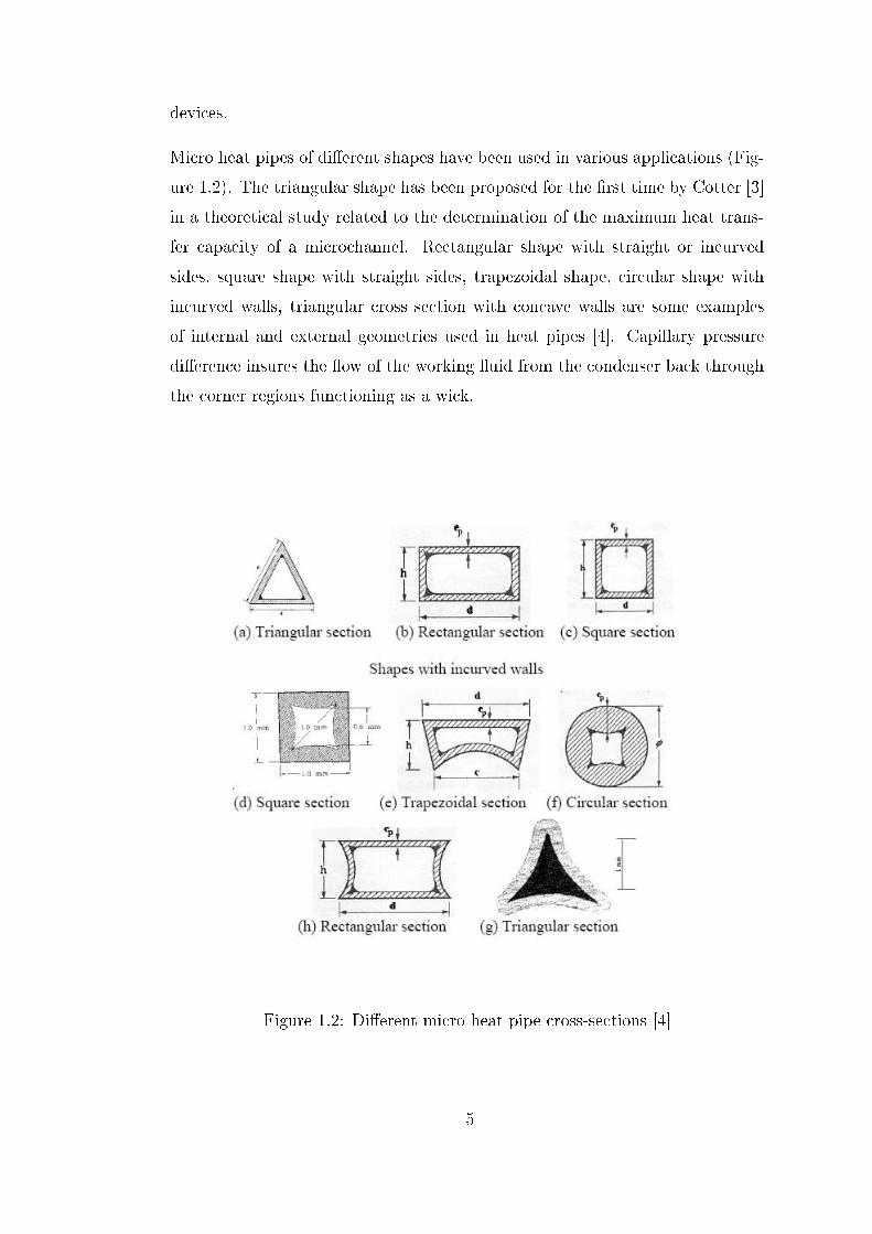
Micro heat pipes of dierent shapes have been used in various applications (Fig-
ure 1.2). The triangular shape has been proposed for the rst time by Cotter [3]
in a theoretical study related to the determination of the maximum heat trans-
fer capacity of a microchannel. Rectangular shape with straight or incurved
sides, square shape with straight sides, trapezoidal shape, circular shape with
incurved walls, triangular cross section with concave walls are some examples
of internal and external geometries used in heat pipes [4]. Capillary pressure
dierence insures the ow of the working uid from the condenser back through
the corner regions functioning as a wick.
Figure 1.2: Dierent micro heat pipe cross-sections [4]
5

1.1.2 Flat heat pipes
Flat heat pipes are similar to traditional cylindrical heat pipes but have a rect-
angular cross-section. They are used to cool and render uniform temperature
distribution on semiconductor or transistor packages assembled in arrays on top
of the heat pipe. For the metallic at mini heat pipes, axial microgrooves with
triangular, rectangular, and trapezoidal shapes are fabricated. Microgrooves
mixed with screen mesh or sintered metal are proposed to improve the perfor-
mance. A number of dierent techniques including high speed dicing and rolling
method, Electric Discharge Machining (EDM), CNC milling process, drawing
and extrusion processes have been applied to fabrication of microgrooves.
Figure 1.3: Construction of at micro heat pipes [5, 6]
1.1.3 Loop heat pipes
Loop heat pipes have separate vapor and liquid lines between the evaporator
and condenser sections. A unique feature of the loop heat pipe is the use of
a compensation chamber which helps maintain the uid inventory. Loop heat
pipes utilize high pumping power allowing heat to be transported for several
meters since loop heat pipes have a wick structure only in the evaporator section.
Loop heat pipes are typically used in aerospace applications and electronics
cooling.
6

Figure 1.4: A typical loop heat pipe [7]
1.1.4 Variable conductance heat pipe
This type of heat pipe maintains the heat source temperature at an almost
constant level over a wide range of heat inputs. This is achieved by maintaining
a constant pressure but at the same time varying the condensation area, which is
called the gas buering. The reservoir, whose volume is much larger than the
heat pipe, is lled with an inert gas. During normal operation the pressure in the
reservoir is equal to the saturation pressure of the uid. When the temperature
of the source increases, the saturation pressure increases and the gas in the
reservoir recedes to increase the condensation area. The applications range from
thermal control of components on satellites to conventional electronics cooling.
7

Figure 1.5: Schematics of a variable conductance heat pipe [8]
1.2 Operational Limits of Heat Pipes
Limitations of the maximum heat input that may be transported by a heat
pipe can be divided into two primary categories, limits that result in heat pipe
failure and limits that do not. For the limitations resulting in heat pipe failure,
all are characterized by insucient liquid ow to the evaporator for a given
heat input, thus resulting in dry-out of the evaporator wick structure. However,
limitations not resulting in heat pipe failure require that the heat pipe operate
at an increased temperature for an increase in heat input. Capillary, boiling
and entrainment limits cause dry-out of the heat pipe. The denitions of the
limitations are summarized in the following sections.
1.2.1 Capillary limit
A liquid droplet on a solid surface has three interfaces, one between the solid
and vapor, a second one between the solid and liquid, and a third one between
the liquid and vapor. There are two types of forces between dierent substances.
8

The forces which act between neighboring parts of the same substance are called
forces of cohesion, and those which act between dierent substances are called
forces of adhesion. These forces are quite insensible when separated by a mea-
surable distance; however, they become perceptible when the distance becomes
exceedingly small. The action between a small size container and a liquid is
named the capillary action. The shape of a liquidvapor interface (meniscus) is
dependent on the liquid's surface tension and the solidliquid adhesion force. If
the adhesion force is greater than the surface tension, the liquid near the solid
will be forced upward. The capillary pressure created by two menisci of dierent
radii of curvature is given by the YoungLaplace equation, where RI and RII
are principal radii of the meniscus surface,
Pc = σ
(1
RI
+1
RII
). (1.1)
In the heat pipe as the liquid in the evaporator vaporizes, the radius of curvature
of the menisci in the wick decreases. The dierence in the radius of curvature
results in capillary pressure dierence, which is the basic driving force for liquid
motion in a heat pipe.
When the capillary forces, developed through the wick structure, are insucient
to drive back enough liquid from the condenser to the evaporator, dry-out occurs
in the evaporator and the heat pipe will fail to operate. Under normal operating
conditions capillary pressure dierence is greater than the total pressure drop
along the heat pipe, which is made up of three components dened below.
• The pressure drop in the liquid phase, 4Pl, required to drive the liquid
from the condenser to the evaporator.
• The pressure drop in vapor the phase, 4Pv, required to cause vapor to
ow from the evaporator to the condenser.
• The pressure due to gravitational head, 4Pg, which may be zero, positive
or negative depending on the inclination of the heat pipe.
The condition dened by the following relation should be satised for proper
9

operation of a heat pipe, otherwise dry-out condition occurs at the evaporator,
4 Pc > 4Pl +4Pv +4Pg. (1.2)
1.2.2 Entrainment limit
In a heat pipe the liquid and vapor ow in opposite directions, whose interaction
results in shear forces at the liquidvapor interface. The magnitude of the force
depends on the vapor properties and velocity, where liquid resists this force by
the surface tension. At high vapor velocities, droplets of liquid in the wick can
be torn from the wick and entrained into the vapor. This results in insucient
liquid ow through the wick structure.
1.2.3 Sonic limit
The sonic limit is typically experienced in liquid metal heat pipes during start-
up or low-temperature operations due to the associated very low vapor densities
under these conditions. With the increased vapor velocities inertial eects of the
vapor ow become signicant, and heat pipe may no longer operate in a nearly
isothermal state, resulting in an increased temperature gradient along the heat
pipe. An analogy between this mode of heat pipe operation and compressible
ow in a converging-diverging nozzle can be made. In a converging-diverging
nozzle, the mass ow rate is constant and the vapor velocity varies due to the
varying cross-sectional area. In heat pipes, however, the ow area is typically
constant and the vapor velocity varies due to mass addition (evaporation) and
mass rejection (condensation) along the heat pipe. As in nozzle ow, decreased
outlet (back) pressure, or in the case of heat pipes, condenser temperatures, re-
sult in a decrease in the evaporator temperature until the sonic limit is reached.
Any further increase in the heat rejection rate does not reduce the evaporator
temperature or the maximum heat transfer capability but only reduces the con-
denser temperature due to the existence of choked ow. The sonic limitation
actually serves as an upper bound to the axial heat transport capacity and does
10

not necessarily result in dry-out of the evaporator wick or total heat pipe failure.
1.2.4 Viscous limit
When the heat pipe operates at low temperatures, the available vapor (satura-
tion) pressure in the evaporator region may be very small to provide required
pressure gradient to drive the vapor from the evaporator to the condenser. In
this case, the total vapor pressure is balanced by opposing viscous forces in the
vapor channel. Thus, the total vapor pressure within the vapor region may be
insucient to sustain an increased ow. This low-ow condition in the vapor
region is referred to as the viscous limit.
1.2.5 Boiling limit
For low values of heat ux, heat is transported to the liquid surface partly by
conduction through the wick and liquid, partly by convection. Evaporation
occurs from the liquid surface. As the heat ux increases, the liquid in contact
with the container wall will be superheated and bubbles will form. With further
increase in the input heat load the wick will dry out and heat pipe stops to
operate.
1.3 Literature Review
In order to better understand the physical mechanism governing the heat and
momentum transfer in heat pipes and to optimize product design, mathematical
models were developed and experiments were conducted. Previous studies are
summarized in the following sections. The summary is organized according
to the wick structure, where the heat pipes with homogeneous or porous wick
structure will be explained rst. Next, the studies on the heat pipes with grooved
wick structure with dierent cross-sections will be summarized. Finally, some
examples about the heat pipes will be given, where the porous and grooved wick
structure are combined to improve the heat removal capacity.
11
1.3.1 Heat pipes with a porous wick structures
A at heat pipe with a porous wick structure is generally composed of a at
container, whose inner side is lined with the wick structure and has a hollow
core for vapor ow. Heat pipes with groove wick structure can only transfer heat
along the groove orientation, however, heat pipes with porous wick structure can
provide heat transfer in any direction. Therefore, they are sometimes referred
as heat spreaders. This property nds wide application in electronics cooling,
where the temperature gradient is reduced and localized hot spots are eliminated.
Homogeneous wick structure also allows cooling of multiple heat sources, such
as integrated heat pipes on electronic boards or chips.
Vafai and Wang [9] analyzed a specic application of a at heat pipe, where it
was used to cool a medical device used in Boron Neutron Capture Therapy. The
heat pipe material was aluminum and the working uid, heavy water. Heat pipe
contained a top and a bottom wick structure and the area for vapor ow was
divided into channels with vertical wicks. An analytical solution is obtained for
the velocity and pressure distribution in the vapor and liquid phases. Clasius
Clapeyron relation was used to obtain the vapor temperature and operating
condition. It was shown that the capillary and boiling limits were not exceeded
and operating temperature was below the operation point of the medical device.
In this application heat source was located at the top center of the heat pipe,
where the remaining area served as the condensation region. It was also shown
that vapor ow was not symmetric and maximum velocity shifted towards the
bottom side due to the vapor injection from the heat source region, whereas the
ow became symmetric away from the heat source region towards the outer sides
of the heat pipe. In [9] vapor ow was analyzed as pseudo-three dimensional
and liquid ow was simulated using Darcy's law. The study on the same heat
pipe conguration was extended by Zhu and Vafai [10] including a nite element
simulation for complete three-dimensional vapor ow and liquid ow including
non-Darcian eect. Studies in [9] and [10] did not include heat transfer anal-
ysis. Wang and Vafai [11] modeled the conduction heat transfer in the heat
pipe container and wick structure in transverse direction for evaporation and
12

condensation regions. A second degree polynomial was assumed for the temper-
ature distribution where the constants were derived using boundary conditions
and an overall heat balance along the heat pipe. This analytical model was
used to predict the transient performance for both the start-up and shutdown
operations. The heat pipe container material was copper, while sintered copper
powder was the wick material and water the working uid. It was shown that
the thermal diusivity of the container and the wick dominated the time for
heat transfer towards the inner side. The ambient heat transfer coecient had
a substantial eect where larger values decreased the time to reach steady state.
The same heat pipe model was investigated by Vafai and Wang [5] experimen-
tally and temperature distribution was measured. The temperature dierence
in the vapor domain was very small and therefore, it was taken as an average
of the evaporation and condensation region end temperatures. Temperature on
the outside surface of the container was measured and it was found that tem-
perature along the condensation area was uniform, whereas the temperature in
the evaporation region was approximately two degrees centigrade higher than
the condensation area. The results also indicated that the porous wick of the
evaporator section created the main thermal resistance resulting in the largest
temperature drop.
Flat heat pipe with the asymmetrical boundary condition in [10, 5] was im-
proved by Faghri and Xiao [12] by including the eect of three-dimensional heat
conduction in the wall, uid ow in the vapor chambers and porous wicks, and
the coupled heat and mass transfer at the liquidvapor interface. The governing
equations for the container, wick and vapor cores were derived and solved by
SIMPLE algorithm. For the vapor region compressible, and for the liquid region
incompressible equations of motion were solved. At the liquidvapor interface
heat balance was used to nd the phase change mass uxes. It was shown that
the vertical wicks improved heat pipe performance by increasing the capillary
pressure. Parametric eects including the heat input and the axial length on
the thermal and hydrodynamic behavior in the heat pipe were investigated.
It was explained that at heat pipes with porous wick structure provide tem-
perature attening for multiple heat sources. Location of the heat source re-
13

gion/regions on the surface of the heat pipe result in a variation of evaporation
and condensation regions according to the application. A simplied analytical
thermaluid model including the container, liquid and vapor ows was devel-
oped for such a heat pipe with four dierent heating and cooling congurations
by Aghvami and Faghri [13]. The congurations were; (i) single heat source and
sink at top, (ii) multiple heat sources and sink at top, (iii) heat source at the
bottom and heat sink on the top, (iv) multiple heat sources and sink positioned
at both the top and bottom of the heat pipe. Two-dimensional steady heat
conduction equation inside the container was solved to obtain the temperature
distribution. Steady, laminar, incompressible ow in vapor and liquid regions
was solved for the axial and transverse velocities and also for the axial pressure
distribution. The results showed that evaporation and condensation are not
conned to the heat source and heat sink regions due to the axial heat transfer
in heat pipe container wall. Therefore, the assumptions that evaporation occurs
only in the heat source region and that condensation occurs only in the heat
sink region, are valid only if the thermal conductivity of the heat pipe container
is very small.
The typical function of a heat pipe is the transfer of heat from a source to a
sink whose locations are xed. In space applications, however, source and sink
positions can be changed for thermal management. Switching source and sink
positions reverses the ow and heat transfer directions and this transient process
was studied by Park et al. [14]. In this case a cylindrical heat pipe with a porous
wick structure was analyzed using the transient, compressible, two-dimensional
ow and heat transfer equations in the vapor region. Wick and container were
included in the analysis in terms of heat transfer, where in the former an eective
thermal conductivity of the wick was dened. Heat sources were dened as
heat ux boundary conditions, whereas in the condensation region convection
and radiation boundary conditions were used. Finite dierence forms of the
governing equations were solved using an in-house developed code. Transition
time after switching the source and sink positions for convection and radiation
boundary conditions were obtained.
Lefevre and Lallemand [15] studied an integrated at heat pipe with several
14

electronic components and heat sinks. Two-dimensional ow model for both the
liquid and the vapor ows were coupled to a three-dimensional thermal model in
the heat pipe container. Constant heat ux was used as boundary condition at
the heat source and heat sink regions. Convection heat transfer coecient was
dened at the outside surface of the heat pipe container. The temperature of
the vapor phase was assumed to be constant and equal to saturation tempera-
ture. Liquid velocity was obtained using Darcy's law whereas the vapor velocity
was obtained assuming the presence of a laminar incompressible ow between
the two parallel plates. This model enabled the calculation of the proportion
of the heat ux, which was conducted through the heat pipe container. It was
shown that the maximum temperature dierence was approximately three times
higher when an equivalent thickness full copper plate was used for cooling. A
similar model was analysed numerically by Sonan et al. [16] and the model was
improved with the inclusion of transient eects. A transient three-dimensional
thermal model was developed to dene the transient heat transfer, both from the
electronic components to the uid and from the uid to the condensers through
the heat pipe container, which was used for the phase change at the container
wick interface. Electronic components were the heat sources, which were mod-
eled by a constant heat ux boundary condition and the condensation regions
were modeled by a convection heat transfer coecient dened between the con-
tainer and the surrounding ambient. In addition, a transient two-dimensional
hydrodynamic model was developed to characterize the uid ow in both the
wick and the vapor core. The simulation was used in the problem of cooling of
three electronic components of a starter generator. The time evolution of max-
imum temperatures over the electronic component were compared to that of an
equivalent solid copper plate. The response time of the heat pipe was faster,
however, it was seen that at maximum power dissipation, the temperature using
the heat pipe was approximately 10oC higher than the copper plate. During
the power descending phase, the maximum temperature with the heat pipe was
about 20oC lower. However, using the heat pipe resulted in a lower temperature
gradient and had lighter weight, which could be preferable in a system design.
Finite element method was applied by Thuchayapong et al. [17] to simulate two-
15

dimensional heat transfer and uid ow at steady state in a heat pipe. The model
included the vapor core, the wick, the container and the water jacket. The results
were compared to experimentally obtained vapor and container temperature
distributions of heat pipes with the coppermesh wick. The results showed that
the capillary pressure gradient inside the wick at the end of the evaporator
section was large which might be attributed to fast liquid motion at the end of
the evaporator section. It was shown that conduction heat transfer dominated
in wick structure except the end of the evaporation section, where high liquid
velocity provided ecient heat transfer through convection and resulted in a
decrease in the wall temperature.
High heat ux values and the restrictions imposed on the size of heat sinks and
fans, and on the noise level associated with the increased fan speed, necessitate
enhanced CPU cooling techniques. Elnaggar et al. [18] simulated a nned U-
shaped heat pipe using ANSYS-FLOTRAN. The evaporation section was located
at the bottom of U-shape in the horizontal position, but the rest constituted
two nned condensation sections in the vertical position, requiring the eect
of gravity to be accounted for. Two-dimensional heat and uid ow equations
were solved to determine appropriate ambient coolant velocity. The results
were compared to experimentally measured container temperatures and coolant
velocity, which were in good agreement.
Heat pipe model studied in [9] was used to investigate the performance improve-
ment eect of nanoparticles in working uid in by Bianco et al. [19]. Nano par-
ticles such as silver, gold, CuO, diamond, titanium, nickel oxide can be added to
the working uid, which change the thermal conductivity, viscosity and density
of the uid. The analytical model used in [9] was modied to include new work-
ing uid properties. Dierent concentrations of Al2O3, CuO, and TiO2 with
diameters of 10, 20 and 40 nanometers were also investigated. It was shown
that nanoparticles reduced thermal resistance of the heat pipe and the liquid
velocity. Wick thickness and nanoparticle concentration levels were optimized
to maximize the heat removal capacity.
16

1.3.2 Heat pipes with grooved wick structures
The concept of micro heat pipe was rst introduced by Cotter [3] and it was
dened as one so small that the mean curvature of the liquidvapor interface is
comparable in magnitude to the reciprocal of the hydraulic radius of total ow
channel. Micro heat pipes do not have wick structure, but non circular chan-
nels serve as liquid arteries. This type of heat pipes also have a wide application
area in electronics cooling, therefore they are investigated both mathematically
and experimentally to understand the operating limitations and the eect of
geometric parameters on their performance. Modeling of a heat pipe requires a
coupled analysis of momentum transfer in the liquid and vapor domains along
with the heat transfer analysis in heat pipe container. Phase change mass ow
rates should be incorporated in both conservation of mass and energy over the
whole domain. Therefore, dierent mathematical approaches were used for mod-
eling. Generally the analyses are not complicated compared to those heat pipes
with homogeneous wick structure and simplied numerical and analytical anal-
yses were performed to understand the overall behavior. Some examples from
the previous studies will be summarized in the following section, where sim-
ple to detailed mathematical modeling approach used in the literature will be
addressed.
The basic assumption in the momentum model is that the ow is steady, unidi-
rectional and incompressible both in the liquid and vapor domains. Total heat
input from the external boundary is used for phase change and conduction in
the heat pipe container is neglected due to the high thermal conductivity of the
solid compared to the working uid. Capillary pressure in the liquid domain is
introduced using YoungLaplace equation and the liquidvapor interface radius
variation along the heat pipe axis is also obtained using this relation. This gen-
eral approach was used by Babin and Peterson [3] to understand the operating
characteristics, where the cross-section of the heat pipe was rectangular but the
internal incurved geometry formed corners which were modeled as triangular
grooves serving as liquid arteries. Capillary limit was the dominant operating
limitation as is the case for other heat pipes, therefore capillary pressure should
17
overcome the pressure losses in the vapor, liquid regions and the hydrostatic
pressure drop. An analytical relation was obtained for total pressure drop and
equalized to capillary pressure to obtain the dry-out limit and maximum heat
transfer capacity. The temperature of the heat pipe container was measured
experimentally and maximum temperature change region was dened as the
beginning of the dry-out region and the analytical results were compared to
experiments.
Micro heat pipes with dierent cross-sections utilize sharp corners for liquid
feed to the evaporation region. These corners can be modeled as triangular
grooves, therefore studies generally concentrate on micro heat pipes having tri-
angular or V-shaped grooves. Peterson and Ma [20] and Khrustalev and Faghri
[21] studied heat transfer capacity of grooves with triangular geometry. Mo-
mentum equations in both liquid and vapor regions were solved using available
correlations. The studies took liquidvapor interfacial shear stress into account
and it was shown that neglecting the shear stress at the free surface of the
liquid due to vaporliquid frictional interaction could lead to an overestima-
tion of the maximum heat transfer capacity. Energy equation was introduced
in the problem where the axial change in mass ow rate was found due to
evaporation and condensation as mentioned in basic assumptions above in [20].
However, Khrustalev and Faghri [21] performed a more detailed analysis, where
condensation and evaporation heat transfer rates were calculated by solving liq-
uid lm thicknesses and conduction through micro liquid regions. The variation
of liquidvapor interface along heat pipe axis, maximum heat capacity, pressure
drops in liquid and vapor regions were obtained. It was shown that as the in-
clination angle and the length of the heat pipe increased, the heat transport
capacity decreased. However, decreasing apex angle of the triangle increased
the heat transport capacity of the heat pipe.
V-shaped groove was modeled by Kumar and Dasgupta [22] where a more de-
tailed evaporation model was applied to obtain evaporation mass ow rates in
transition and meniscus regions and results were reported for dierent heat input
values. In this study, heat balance at macro level was written for a unit liquid
volume, where the dierence between the inow and evaporation heat transfer
18

was used to increase the liquid temperature axially. The change of the liquid
vapor interface radius was investigated for dierent values of heat input. The
eects of inclination and apex angle on the heat capacity of the heat pipe were
studied. The decrease in apex angle resulted in an increased liquidvapor inter-
face radius change and hence improved capillary pumping, resulting in higher
heat transfer capacity.
Suman and DasGupta [23] generalized the uid ow model for any arbitrary
(polygonal) shaped groove. However, the detailed evaporation mass transfer
model given in [22] was not used in this study. In addition, macro level heat
balance for a unit liquid volume did not consider the axial temperature distri-
bution. The numerical model used in the solutions of grooved heat pipes with
triangular and rectangular cross-sectional geometries. In this case, the axial
variation of liquidvapor interface radius was used to predict the onset of the
dry-out point and the propagation of the dry-out length, where the minimum
value of the radius at the end of the evaporation region is dened by the contact
angle and the geometry of the cross-section. It was shown that triangular heat
pipes have higher heat carrying capacity with respect to rectangular ones. Simi-
lar analysis was conducted by Suman and Hoda [24], where the eect of contact
angle, surface tension and viscosity of the working uid, inclination, apex angle
of V-groove, length of adiabatic section on the heat removal capacity of the heat
pipe were studied.
The modeling approach in [23] was extended to include the transient eects by
Suman et al. [25]. The triangular micro-heat pipe was taken as a test case. The
coupled equations of heat, mass and momentum transfer were solved to obtain
the transient as well as the steady state proles of temperature. It was shown
that higher heat input required more time to reach steady state.
Experiments were carried out to study the onset and propagation of dry-out
point on a silicon surface with V-shaped grooves where pentane was used as
the working uid by Anand et al. [26]. The axial temperature distribution was
accurately measured as a function of the heat input and inclination without the
working uid in the heat pipe. Since no working uid at dry-out point was
19
present, the temperature distribution during the operation of the heat pipe was
compared to the measured temperature without the working uid. Where these
two temperatures coincide, it was noticed that dry-out point was reached. The
problem was also solved numerically using an approach similar to [23] to predict
the onset, location and propagation of the dry-out point. The results showed
that by increasing inclination angle and heat input, dry-out point propagated
away from the heat input region.
Shear stress at the liquidvapor interface contributes to the increase of the liq-
uid pressure drop and decreases the heat transfer capacity of the heat pipe.
Generally, heat pipe analysis uses predened correlations to include this eect.
Thomas et al. [27] studied fully developed laminar ow for one cross-section
in a trapezoidal groove. A correlation for shear stress was dened in terms of
Poiseuille number (f · Re) as a function of groove aspect ratio, groove half an-
gle and liquid contact angle. A semi-analytical solution for capillary limit was
obtained.
Launay et al. [28] developed a mathematical model for predicting the heat
transport capacity and temperature distribution along the axial direction of a
triangular heat pipe, lled with water. A detailed evaporation and condensation
model from kinetic theory was utilized and lm thickness along evaporation
and condensation micro regions were obtained, which were used to calculate
thermal resistance and the heat transfer rate through the liquid lm. An iterative
procedure in terms of vapor temperature was applied, where heat transferred
from the condensation region became equal to the dened heat input at the
evaporation region. In this study heat pipe container temperature was also
obtained using detailed evaporation and condensation models. Ratios of heat
transferred in the evaporator and condenser regions showed that the geometry
of the micro region could be altered to increase the heat removal capacity of
the heat pipe. The velocity, pressure, and temperature distributions in the
vapor and liquid phases were calculated. Fluid ll charge eect on heat pipe
heat removal capacity was predicted and it was shown that ll ratio should be
optimized to obtain maximum heat removal capacity for a given heat input.
20
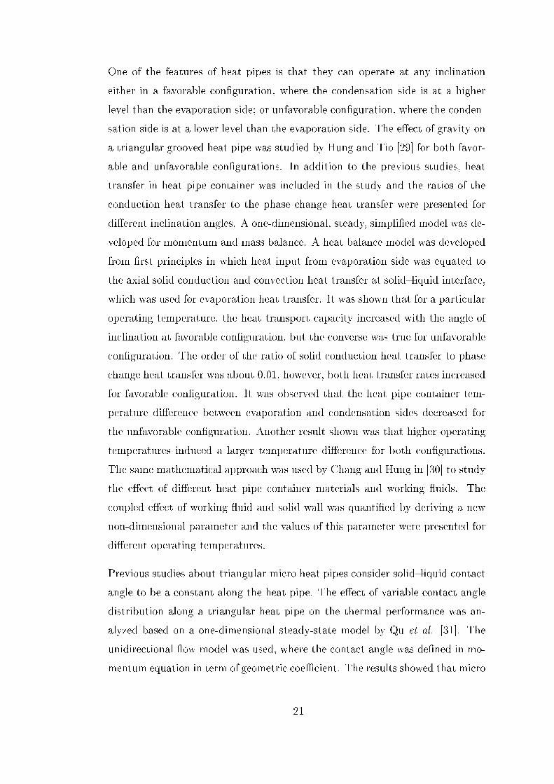
One of the features of heat pipes is that they can operate at any inclination
either in a favorable conguration, where the condensation side is at a higher
level than the evaporation side; or unfavorable conguration, where the conden-
sation side is at a lower level than the evaporation side. The eect of gravity on
a triangular grooved heat pipe was studied by Hung and Tio [29] for both favor-
able and unfavorable congurations. In addition to the previous studies, heat
transfer in heat pipe container was included in the study and the ratios of the
conduction heat transfer to the phase change heat transfer were presented for
dierent inclination angles. A one-dimensional, steady, simplied model was de-
veloped for momentum and mass balance. A heat balance model was developed
from rst principles in which heat input from evaporation side was equated to
the axial solid conduction and convection heat transfer at solidliquid interface,
which was used for evaporation heat transfer. It was shown that for a particular
operating temperature, the heat transport capacity increased with the angle of
inclination at favorable conguration, but the converse was true for unfavorable
conguration. The order of the ratio of solid conduction heat transfer to phase
change heat transfer was about 0.01, however, both heat transfer rates increased
for favorable conguration. It was observed that the heat pipe container tem-
perature dierence between evaporation and condensation sides decreased for
the unfavorable conguration. Another result shown was that higher operating
temperatures induced a larger temperature dierence for both congurations.
The same mathematical approach was used by Chang and Hung in [30] to study
the eect of dierent heat pipe container materials and working uids. The
coupled eect of working uid and solid wall was quantied by deriving a new
non-dimensional parameter and the values of this parameter were presented for
dierent operating temperatures.
Previous studies about triangular micro heat pipes consider solidliquid contact
angle to be a constant along the heat pipe. The eect of variable contact angle
distribution along a triangular heat pipe on the thermal performance was an-
alyzed based on a one-dimensional steady-state model by Qu et al. [31]. The
unidirectional ow model was used, where the contact angle was dened in mo-
mentum equation in term of geometric coecient. The results showed that micro
21

heat pipe with variable contact angle could remove a larger amount of heat for
a given heat input. Increased thermal performance could be attributed to the
increase in the liquid capillary force, however, it was observed that there was no
perceptible increase in the liquid shear force.
Grooved heat pipes with dierent cross-section proles were also investigated
such as Ω-shaped [32] or dual cored trapezoidal grooved [33] and trapezoidal
grooved [34] cylindrical heat pipes.
A theoretical model of uid ow and heat transfer with axial Ω-shaped grooves
was studied for maximum heat transport capability by Chen et al. [32]. The
inuence of variations in the liquidvapor inteface radius, interfacial shear stress
and the contact angle were considered. The axial distribution of the liquid
vapor inteface radius, uid pressure and mean velocity were obtained where the
accuracy of the developed model was veried by experimental data.
Among the heat pipes with dierent wick structures like wire mesh, arteries,
foams, axial grooves, and porous materials, axially grooved heat pipes are proven
to be reliable for long-life spacecraft missions. Dual core axially trapezoidal
grooved aluminum heat pipe using ethane as working uid was chosen for satel-
lite thermal control by Anand et al. [33]. Flow equations for liquid and vapor
cores were considered for maximum heat transport capacity and the results of
the analysis were also veried by experimental study.
A mathematical model for heat and mass transfer in a cylindrical heat pipe
with trapezoidal grooved structure was solved analytically by Kim et al. [34].
The eects of the liquidvapor interfacial shear stress, contact angle, and the
amount of initial liquid charge were considered in the proposed model. Modi-
ed Shah method was suggested and validated for liquidvapor interfacial shear.
For the heat transfer equation, thermal resistances in solid and liquid regions,
simplied models for evaporation and condensation by dening eective heat
transfer coecients were used. Analytical results for the maximum heat trans-
port rate and total thermal resistance were shown to be in close agreement with
the experimental results.
22

Viscous losses in grooved heat pipes limit the heat transport capacity, which is
less than that of a homogeneous wicked heat pipe. The electrohydrodynamic
(EHD) pumping oers a promise to improve the capacity with a smaller size,
which is a concern whenever size limitation is imposed. The EHD phenomenon
involves the interaction of the electrical eld and the ow eld in a dielectric uid
medium. This interaction can result in electrically induced uid motion that is
caused by an electrical body force. V-grooved micro heat pipe was studied by
Suman [35], where an electrical body force was added in the momentum equation
of the working uid. Analytical expressions for the critical heat input and dry-
out lengths were obtained, which showed that the critical heat input increased
and the dry-out length decreased with increasing applied electrical eld.
Theoretical modeling of a triangular micro-heat pipe showed that the heat trans-
port capacity increases when the channel apex angle and the length of the
micro-heat pipe decreases. Star-grooved heat pipes obtain the desired corner
apex angle without aecting the number of corners, therefore, under identical
operating conditions star-grooved micro-heat pipe reveal better performance.
The study by Hung and Seng [36] considered a one-dimensional, steady-state
mathematical model, where the continuity, momentum, and energy equations of
the liquid and vapor phases, together with the YoungLaplace equation, were
solved numerically to yield the heat and uid ow characteristics of the micro
heat pipe.
Chauris et al. [37] analyzed a at heat pipe, where lower, upper and vertical
sides contain triangular grooves, whereas the intersection between horizontal
and vertical sides were combined through droplet shaped grooves at the corners.
Simple mathematical models for momentum model and mass balance were used
and heat input was used to nd liquidvapor interface velocity. Dierent work-
ing uids were studied to investigate dry-out length as a function of working
temperatures.
Flat heat pipes having rectangular groove arrays were investigated by various
authors [38, 39]. A mathematical model was developed for predicting the ther-
mal performance of a at micro heat pipe with a rectangular groove by Do et al.
23

[38]. Generally, heat pipe calculations were carried out with the following as-
sumptions: (i) evaporation and condensation were assumed to occur uniformly
in the axial direction; (ii) neither evaporation nor condensation occurred in the
adiabatic section inside the heat pipe; (iii) the container temperature was either
assumed to be constant or its variation was neglected. These simplifying assump-
tions had good applicability to small heat pipes, whereas experiments showed a
temperature drop of 25C for a length of 120 mm. This suggested that the axial
variation of the container temperature and the evaporation and condensation
rates should be taken into consideration. Therefore, the axial variation of the
container temperature was accounted for in the energy balance equation. The
evaporation and condensation mass ow rates were calculated from the relations
obtained from kinetic theory and conduction through the liquid region. The ef-
fects of the liquidvapor interfacial shear stress, contact angle, and the amount
of liquid charge were included in this model. Numerical results were found to be
in good agreement with those given in [40]. Finally, the grooved wick structure
was optimized for maximum heat transport rate as a function of the width and
the height of the groove.
Two-phase heat spreaders with rectangular grooves have a high evaporation area
compared to the condensation area. A one-dimensional two-phase ow model
was developed for such a heat spreader in horizontal orientation by Rulliere et al.
[41]. A confocal microscope was used to measure the liquidvapor interface
radius along the groove. The measurements were compared to the results of
uid ow model based on mass and momentum balance and the YoungLaplace
equation. Container temperatures were measured with three dierent working
uids, namely water, n-pentane and methanol. The experimental results were
found to be in good agreement with the calculated liquidvapor interface radii
that were obtained without considering interfacial shear stress, since vapor cross
section was larger than liquid cross section in this heat pipe. A similar analysis
was performed by Lefevre et al. [6], where the heat conduction in each cross
section in liquid and solid regions was solved to obtain the thermal resistance,
which was used to nd the axial temperature distribution along the heat pipe
container. The results were validated in experiments, in which liquidvapor
24
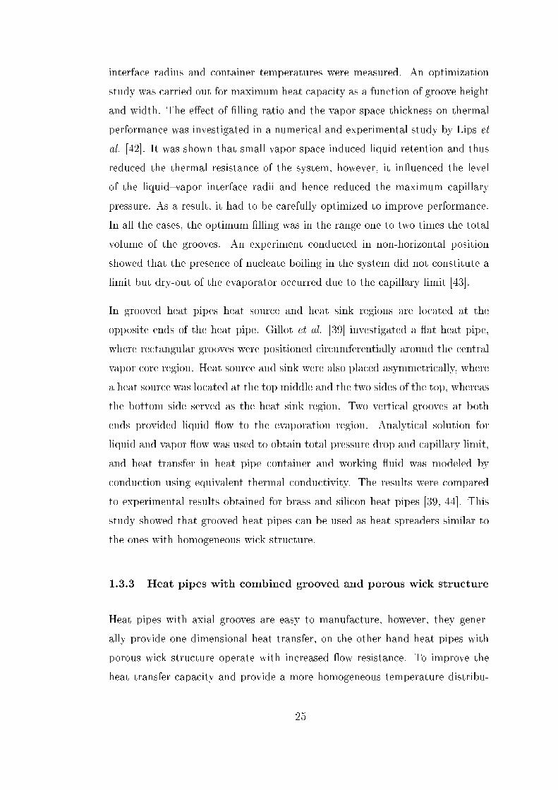
interface radius and container temperatures were measured. An optimization
study was carried out for maximum heat capacity as a function of groove height
and width. The eect of lling ratio and the vapor space thickness on thermal
performance was investigated in a numerical and experimental study by Lips et
al. [42]. It was shown that small vapor space induced liquid retention and thus
reduced the thermal resistance of the system, however, it inuenced the level
of the liquidvapor interface radii and hence reduced the maximum capillary
pressure. As a result, it had to be carefully optimized to improve performance.
In all the cases, the optimum lling was in the range one to two times the total
volume of the grooves. An experiment conducted in non-horizontal position
showed that the presence of nucleate boiling in the system did not constitute a
limit but dry-out of the evaporator occurred due to the capillary limit [43].
In grooved heat pipes heat source and heat sink regions are located at the
opposite ends of the heat pipe. Gillot et al. [39] investigated a at heat pipe,
where rectangular grooves were positioned circumferentially around the central
vapor core region. Heat source and sink were also placed asymmetrically, where
a heat source was located at the top middle and the two sides of the top, whereas
the bottom side served as the heat sink region. Two vertical grooves at both
ends provided liquid ow to the evaporation region. Analytical solution for
liquid and vapor ow was used to obtain total pressure drop and capillary limit,
and heat transfer in heat pipe container and working uid was modeled by
conduction using equivalent thermal conductivity. The results were compared
to experimental results obtained for brass and silicon heat pipes [39, 44]. This
study showed that grooved heat pipes can be used as heat spreaders similar to
the ones with homogeneous wick structure.
1.3.3 Heat pipes with combined grooved and porous wick structure
Heat pipes with axial grooves are easy to manufacture, however, they gener-
ally provide one dimensional heat transfer, on the other hand heat pipes with
porous wick structure operate with increased ow resistance. To improve the
heat transfer capacity and provide a more homogeneous temperature distribu-
25

tion in any direction some novel design prototypes were proposed and studied.
One example is the heat pipe produced and investigated both analytically and
experimentally by Wang and Peterson [45]. Copper screen mesh was used as the
primary wicking structure, in conjunction with a series of parallel wires, which
formed liquid arteries where water was selected as the working uid. Capillary,
boiling, entrainment limitations were investigated through empirical relations
considering heat input and geometric parameters. Two prototypes were tested
experimentally and maximum heat removal capacity results were found to be
in good agreement with empirical results. Increasing the wire diameter resulted
in an increase in the maximum heat transport capacity. The mesh number had
conicting eects on the capillary pumping capacity and the frictional pressure
drop, i.e. increasing mesh number provided higher capillary force, however, also
resulted in higher pressure drop. Therefore, optimum design parameters should
be searched for a specic operating temperature. Similar to the mesh number,
the wick thickness had an opposing eect on the capillary and boiling heat trans-
fer. As the wick thickness increased liquid pressure drop decreased due to larger
area, but it reduced boiling limit, where the liquid was easily superheated. The
inclination angle had a dominant eect on the maximum heat transfer capacity,
as the heat transport capacity decreased with increasing inclination angle.
Rectangular grooved at heat pipe mentioned in [38] was extended by Do and
Jang [46] by adding water-based Al2O3 nanouids as the working uid. The
nanoparticles increased thermal conductivity of the working uid, but also ac-
cumulated on the heat transfer surface in the evaporation region. This porous
layer enhanced evaporation heat transfer and the driving capillary force. Ax-
ial momentum equations in the liquid and vapor were solved, where eective
density and viscosity values were dened by considering the volume fraction of
nanoparticles. Evaporation and condensation mass uxes for each cross-section
along the heat pipe axis were calculated by the relations obtained from kinetic
theory, where the thermal conductivity of the liquid was recalculated due to the
addition of nanoparticles. Due to nanoparticle coating in evaporation region,
one additional relation from kinetic theory and Darcy's law was obtained for
the evaporation region on the n top. The eects of the volume fraction and
26

the size of nanoparticles on the thermal performance were studied, where results
showed that adding less than 1% nanouids enhanced thermal performance up
to 100%.
1.4 Description of the Current Study
As summarized in the previous section, numerous studies have been performed
on heat pipes to compute the maximum heat removal capacity and get an insight
to the physical mechanisms involved. The eects of the physical and geometrical
parameters (groove size, contact angle, shear force at the liquidvapor interface)
were investigated for geometries with dierent cross section. For at heat pipes
with porous wick, detailed analyses were performed for momentum equation
both in liquid and vapor regions and heat transfer in the container. For grooved
micro heat pipes the analyses were less detailed, simplifying assumptions and
pre-dened correlations for solidliquid and liquidvapor interface shear stresses
were used. Temperature distribution along the heat pipe container was not con-
sidered generally and evaporation and condensation mass ow rates correlated
through heat input to the evaporator. Studies on at grooved heat pipes with
rectangular cross-section included axial temperature distribution through the
heat transfer equation in the heat pipe container and working uid by dening
thermal resistances and using electrical analogy. Evaporation and condensation
mass uxes were found from correlations available in the literature or dened
heat transfer coecient at the liquidvapor interface.
In the present study a at micro heat pipe with rectangular cross section is
investigated. Three dimensional heat transfer equation both in the heat pipe
container, solid domain, and in the working uid, liquid domain, is solved, which
is coupled to the evaporation and condensation models at the liquidvapor in-
terface. Evaporation and condensation models are used to dene the liquid lm
thickness along the micro region, which is used to nd the phase change mass
uxes at each cross-section along the heat pipe. The details of the modeling will
be presented in Chapter II.
27
The shape of the interface between liquid and vapor is not known a priori and
each cross-section is assumed to be circular. Since the physical domain is irregu-
lar in the liquid domain, a coordinate transformation is made and a transformed
form of the heat transfer equation is obtained for a xed rectangular computa-
tional domain, which is used in the numerical solution. Heat transfer equation
in the liquid domain includes the eect of convective heat transfer, which is
generally neglected and the eect of the convection on heat pipe performance is
investigated.
The axial ow is modeled as a one dimensional incompressible ow where the
averaged velocity is used at each cross section. Shear force between solidliquid
interface is dened by an empirical relation. YoungLaplace equation is used to
correlate surface tension and the liquidvapor interface radius to pressure drop
in the liquid domain.
The details of the solution methodology will be explained in Chapter III. Chapter
IV includes validation of the current model with the results of Lefevre et al. [6]
as well as a parametric study considering the eect of the dimensions of the
heat pipe geometry and boundary conditions on the heat removal capacity of
the heat pipe. A sample problem simulating cooling of an electronic component
is solved in Chapter V to design a heat pipe with a given set of design objectives
and restrictions.
28
CHAPTER 2
PHASE CHANGE
Heat pipes take advantage of phase change heat transfer to remove large amounts
of heat in small areas with small temperature dierences. Evaporation and
condensation modeling is a major area of interest in heat pipe research and a
detailed explanation of evaporation and condensation modeling will be given in
this chapter and the comparison of the present model with the previous studies
will be presented.
2.1 Evaporation Modeling
Evaporation is a surface phenomenon, where the liquid molecules with sucient
energy to overcome intermolecular forces at the liquidvapor interface escape
from the bulk liquid region and change state to gaseous phase. If evaporation
takes place in an enclosed area, the escaping molecules accumulate as a vapor
above the liquid and many of the molecules return to the liquid. When the
process of escape and return reaches equilibrium, the vapor state is saturated.
For a system consisting of vapor and liquid of a pure substance, this equilibrium
state is related to the vapor pressure by the ClausiusClapeyron relation,
ln
(P2
P1
)= −hlv
Ru
(1
T2− 1
T1
), (2.1)
where P1 and P2 are vapor pressures at temperatures T1 and T2, Ru the universal
gas constant and hlv the latent heat of evaporation.
29

At the liquidvapor interface the conservation of mass, momentum and energy
should be satised. Momentum equation at the interface reduces to Young
Laplace equation, since the momentum terms due to interface motion are small,
Pl − Pv =σ
R, (2.2)
where R is the radius at the liquidvapor interface and σ is the surface tension
of the liquid. The denition of the capillary pressure was given in Equation
1.1 by two principal radii of liquidvapor interface, however, the radius in axial
direction is very large compared to the one along the groove cross-section and
it's contribution is neglected in Equation 2.2.
Conservation of energy at the interface requires
q′′l − q′′v = m′′ehlv (2.3)
where q′′l and q′′v are heat uxes at liquid and vapor sides and m′′e is evaporation
mass ux at the interface.
When the evaporator section of a grooved heat pipe is analyzed, three subregions
of the evaporating lm section can be observed (Figure 2.1).
• the adsorbed lm/non-evaporating region, where the liquid layer is thin,
of the order of a fraction of nanometers and remains constant. There is no
mass transfer, since intermolecular interactions between the wall and the
liquidvapor interface dominate,
• evaporating thin lm region, where both the intermolecular and capillary
forces are dominant,
• meniscus/macro region, where intermolecular forces are negligible, and the
curvature of the interface becomes constant. In this zone, the liquid layer is
too thick to be inuenced by the liquidsolid interactions. The equilibrium
is mainly governed by the capillary forces.
30

The rst two regions are called the micro-region which forms a very small
portion of the global meniscus. However, this region is characterized by high
heat transfer rates due to the very low resistance to heat transfer across the
liquid lm. It was shown that liquidvapor interface curvature is not constant
Fluid Flow
B
A
C
A: non-evaporating region
B: evaporating thin film region
C: meniscus/macro region
micro region
Eva
po
ratio
n
Figure 2.1: Evaporation micro region and subregions
and the interface temperature is greater than the saturation temperature in the
micro region [47]. Transverse pressure gradient in liquid phase results in large
curvatures in this region, which decrease the volatility of the liquid and increases
the interface temperature above the saturation temperature.
The coordinate system used for the micro region evaporation model is given in
Figure 2.2. The origin of the coordinate system is placed at the interface between
the evaporating thin lm region and meniscus regions. The axial direction, s,
extends to the non-evaporating region and transverse direction, n, extends from
the liquid to vapor phase.
31

s
Non-evaporating
region
Evaporating
thin-film region
Meniscus/macro
region
n
Liquid film thickness
Contact angle
Figure 2.2: Coordinate system used in the evaporating region
The liquid ow in the axial direction compensates the evaporation mass ux
from thin lm region as shown in Figure 2.1. Evaporation mass ux in the
evaporating thin lm region can be dened from kinetic theory as in Equation
2.4,
m′′e = a (Tlv − Tv) + b (Pl − Pv) , (2.4)
where
a =2c
2− c
(M
2πRuTlv
)1/2(MPvhlvRuTvTlv
), (2.4a)
b =2c
2− c
(M
2πRuTlv
)1/2(PvVlRuTlv
), (2.4b)
where c is the accommodation coecient, hlv is the latent heat of evaporation,
M is the molecular weight, Ru universal gas constant, V molar volume of liquid
32

phase, Pv vapor pressure, Pl liquid pressure, Tv vapor temperature, and Tlv
liquidvapor interface temperature.
There are two contributions to the pressure dierence between the liquid and
vapor phases, which are due to the eects of dispersion and surface tension as
represented in Figure 2.3.
Vapor Pressure, vP
Dispersion Pressure, dP
Liquid Pressure, lP
Capillary Pressure, cP
Figure 2.3: Pressure balance at the liquidvapor interface
Dispersion pressure in the micro region comprises several components which
include the molecular component, electrostatic component (existing in ionic so-
lutions) and structural component which is related to the formation of the hy-
dration layers of polar molecules near interfaces [48]. For a non-polar liquid, the
dispersion pressure can be expressed as,
Pd =Adδ3, (2.5)
where Pd , is the dispersion constant and, δ, is the liquid lm thickness. For polar
33

liquids like water and aqueous solutions logarithmic functions from experimental
studies are also used to represent the dispersion pressure.
Capillary pressure is dened in terms of curvature of the liquidvapor interface
(Equation 2.6).
Pc = σd 2δ/ds 2(
1 + (dδ/ds)2)3/2 (2.6)
The dierence between the vapor and liquid pressures is balanced by the disper-
sion and capillary pressures at the interface,
Pv − Pl = Pd + Pc. (2.7)
By dierentiating Equation 2.7 with respect to s, which is the coordinate dened
from the meniscus region to the non-evaporating region (Figure 2.2), the varia-
tion of liquid pressure in terms of liquid lm thickness, δ, is obtained assuming
that the vapor pressure is constant.
dPlds− 3Ad
δ4dδ
ds+ σ
d 3δ/ds 3(1 + (dδ/ds)2
)3/2 − 3σ(d 2δ/ds 2)
2((1 + (dδ/ds)2
)5/2 dδds (2.8)
The liquid feed from the macro region can be formulated as a fully developed
one-dimensional ow in the s-direction as given in Equation 2.9,
dPlds
= µd 2uldn2
, (2.9)
subject to the boundary conditions,
dul/dn = 0 at n = δ, (2.9a)
ul = 0 at n = 0, (2.9b)
Mass ow rate at each cross section can be obtained through the integration,
m′e = ρl
∫ δ
0
ul dn (2.10)
34

Dierentiating Equation 2.10 with respect to s and combining with Equation 2.8
the mass ux along the direction of ow, m′′e , becomes,
− d
ds
(δ3
3ν−(
3Adδ4
dδ
ds+σ
d 3δ/ds 3(1 + (dδ/ds)2
)3/2 −3σ(d 2δ/ds 2)
2(1 + (dδ/ds)2
)5/2 dδds))
(2.11)
Evaporation mass ux can be obtained from Equation 2.4, however as mentioned
before liquidvapor interface temperature is higher than the saturation temper-
ature and is also an unknown. Therefore, the heat ux between liquidvapor
interface and heat pipe wall is used to dene the interface temperature.
m′′e = a (Tlv − Tv) + b (Pl − Pv) = klTw − Tlvδhlv
(2.12)
Tlv =klTw/δhlv + aTv + b (Pv − Pl)
a+ kl/δhlv(2.13)
Evaporation mass ux is written in terms of the heat pipe wall temperature, so
Equation 2.4 becomes
m′′e =a(Tw − Tv) + b(Pl − Pv)
1 + aδhlv/kl(2.14)
Equations 2.11 and 2.14 are rearranged to give Equation 2.15 and integrated to
obtain the liquid lm thickness and evaporation mass ux at each cross section
of the micro region.
d
ds
(δ3
3ν−(
3Adδ4
dδ
ds+ σ
d 3δ/ds3(1 + (dδ/ds)2
)3/2 − 3σ(d 2δ/ds2)
2(1 + (dδ/ds)2
)5/2 dδds))
= −a(Tw − Tv) + b(Pl − Pv)1 + aδhlv/kl
(2.15)
subject to following boundary conditions.
δ = δ0 at s = 0, (2.15a)
35

dδ/ds = − tan θ at s = 0, (2.15b)
Pv − Pl =σ/R at s = 0, (2.15c)
d (Pv − Pl) /ds = 0 at s = 0, (2.15d)
m′′e = 0 at s = l. (2.15e)
Since the total length of the evaporating region is not known a priori, one addi-
tional condition should be introduced to nd the length, l, dened in Equation
2.15.e.
Assuming that dispersion pressure is 1/100000th of the capillary pressure at the
beginning of the coordinate system, i.e s = 0,
Pd =σ
R10−5 =
Adδ30
(2.16)
the initial value of the liquid lm thickness, δ0, can be found.
The heat transfer in micro grooves and heat pipes were investigated by several
authors to nd out the evaporating heat transfer coecient and the eect of the
physical and geometric parameters on evaporation heat transfer performance.
Stephan and Busse [47] modeled the evaporator section of a trapezoidal grooved
heat pipe. The study shows that the liquidvapor interface temperature is higher
than the saturation temperature. In this study, liquid lm thickness, interface
temperature and heat ux variation along the micro region were calculated and
the ratio of micro region evaporation heat transfer to the liquid meniscus region
was also reported. A similar analysis was performed by Bertossi [49] and dif-
ferent working uids were compared in terms of micro region evaporation rates.
The denition of micro region can be dierent according to the assumptions
and related boundary conditions to formulate the micro region evaporation. Du
and Zhao [48] studied the problem by dening a new boundary condition and
compared their results to the previous studies. A mathematical model was de-
veloped by Jiao et al. [50] to investigate the eect of thin lm evaporation on
the maximum heat capacity of a trapezoidal micro-grooved heat pipe. The ef-
fect of the contact angle on meniscus radius, heat transfer rate and micro region
36

length was investigated. It was shown that contact angle increase results in a
nonlinear increase in the meniscus radius and a decrease in the length of the
micro region. This results in a decrease in the heat transfer capacity through
the micro region. A similar model was developed by Cheng et al. [51] to deter-
mine the heat transfer through both the thin-lm and liquid meniscus regions
in a rectangular microgroove. In the liquid meniscus region two-dimensional
steady heat conduction equation was solved analytically to determine the heat
transfer rate. It was shown that the contribution of heat transfer through the
liquid meniscus region depended on the contact angle and solid wall superheat.
Present study, where the details were explained in the previous paragraphs, is
compared to the results of [47] in terms of liquid lm thicknesses and heat uxes
in the micro region. The working uid in [47] was ammonia and other physical
parameters used in the analysis are given in Table 2.1
Table 2.1: Physical parameters used in evaporation model
Vapor temperature (K) Tv 300
Vapor pressure (Pa) Pv 1.06× 10⁵
Latent heat of evaporation (J/kg) hlv 1.18× 10⁻⁶
Density of liquid (kg/m3) ρ 600
Surface tension (N/m) σ 2.0× 10⁻²
Thermal conductivity (W/m ·K) kl 0.48
Molar mass of liquid (kg/mol) M 17.3× 10⁻³
Molar volume of liquid (m3/mol) Vl 28.8× 10⁻⁶
Accommodation coecient c 1
Dispersion constant (J) Ad 2.0× 10⁻²¹
Interface radius (m) R 909× 10−6
Film thickness variation along the micro region is shown in Figure 2.4. There is
a 5% dierence between the present study and the results of Stephan and Busse
37

[47]. Heat ux variation is given in Figure 2.5, where the maximum value of
both results coincide. It is given in [47] that the overall heat transfer in a span
of 1µm region is 6.6 W, whose value in the present study is 7.52 W.
0.0E+00
2.0E-08
4.0E-08
6.0E-08
8.0E-08
1.0E-07
1.2E-07
1.4E-07
0.0E+00 1.0E-07 2.0E-07 3.0E-07 4.0E-07 5.0E-07 6.0E-07
Micro region, s (m)
Fil
m t
hic
kn
ess,
d (m
)
Results of Stephan & Busse
Present study
Figure 2.4: Liquid lm thickness variation along the micro region
38

0.0E+00
1.0E+07
2.0E+07
3.0E+07
4.0E+07
5.0E+07
6.0E+07
0.0E+00 1.0E-07 2.0E-07 3.0E-07 4.0E-07 5.0E-07 6.0E-07
Micro region, s (m)
Heat
flu
x,
q (
W/m
2)
Results of Stephan & Busse
Present study
Figure 2.5: Heat ux variation along the micro region
2.2 Condensation Modeling
Condensation is the change of the state from gaseous phase into liquid phase, and
is the reverse of evaporation. Most of the condensation occurs at the top of the
n, which can be dened as the micro region for condensation. A schematic of
the condensation on the top of the n is represented in Figure 2.6. Condensation
mass ux is dened in a way similar to the evaporation mass ux using kinetic
theory. However, in this case dispersion pressure in the liquid region is neglected.
Equation 2.15 given for evaporation is rewritten for condensation in the following
form,
σ
3ν
d
ds
(δ3d3δ
ds3
)= −a(Tw − Tv) + b(Pl − Pv)
1 + aδhlv/kl(2.17)
39

Condensation
Liquid
flow Liquid film
thickness
s
Fin
thickness t
Figure 2.6: Condensation region and the groove geometry
The pressure dierence between the vapor and liquid phases is made up of
only the capillary pressure. The variation of lm thickness along the n top is
small, therefore the derivative in the thin lm curvature denition can also be
neglected. The pressure jump at the liquidvapor interface is given in terms of
lm thickness, δ,
Pv − Pl = σd 2δ
ds 2(2.18)
The boundary conditions for the lm thickness are
dδ/ds = dδ3/ds3 = 0 at s = 0, (2.18a)
dδ/ds = − tan θ at s = t, (2.18b)
d2δ/ds2 = 0 at s = t. (2.18c)
The boundary conditions given in Equations 2.18ac for the liquid lm thickness
40

along the n top and the mass balance, where the condensed uid mass is
equal to total mass ow rate from the n, should be satised. In this case
the dierential equation for the lm thickness is not solved but an integral
approach is adopted using a fourth degree polynomial t satisfying the boundary
conditions to approximate the lm thickness,
δ = c0 + c1(s− t) + c2(s− t)2 + c3(s− t)3 + c4(s− t)4. (2.19)
The coecients c1 − c4 are obtained using the boundary conditions dened in
Equations 2.18ac.
c1 = − tan (π/2− θ) (2.19a)
c2 = 0 (2.19b)
c3 = c1/2t2 (2.19c)
c4 = c1/ (2t)3 (2.19d)
The condition, where total mass ow rate along the n top is equal to the
condensation mass ow obtained using the kinetic theory, is used to calculate
the unknown coecient c0 in Equation 2.19. The left hand side of Equation 2.17
is integrated analytically to obtain the total mass ow,
σ
3ν6 c30 c3 = m
′
c. (2.20)
Heat ux at the liquid vapor interface is used to dene the interface temperature,
which is substituted into Equation 2.22.
Tlv = Tw +m′′chlvδ
kl(2.21)
An iterative procedure is applied to obtain the constant c0 which satises Equa-
tion 2.22.
m′c +
∫ t
0
a(Tw − Tv) + b(Pl − Pv)1 + aδhlv/kl
ds = f (2.22)
41

After the lm thickness variation dened by the fourth degree polynomial is
obtained, the condensation mass ow is calculated from Equation 2.17.
Y. Zhang and A. Faghri [52] modeled a rectangular groove and studied the
condensation at the n top using the Volume of Fluid (VOF) method. Two di-
mensional incompressible momentum equation in a groove was solved along with
the condensation at the n top. The model included only one cross section of
a grooved heat pipe, where the groove wall temperature had a xed value. The
eects of surface tension, wall temperature, contact angle at the solidliquid
interface and n thickness were investigated. Numerical simulation was per-
formed for water at the saturation temperature of 373 K. It was concluded that
the liquid lm on top of the n became atter and the heat transfer coecient
on the n top became more uniform when the contact angle increased. It was
also observed that the heat transfer coecient decreased with increasing tem-
perature dierence between the groove wall and the liquid vapor temperature.
Increasing surface tension decreased liquid lm thickness and as a result heat
transfer coecient increased. The results of the present study are compared to
the results of [52]. The physical parameters used in the comparison calculation
are given in Table 2.2.
The results are compared for lm thickness and heat ux variation along the
n top, where the contact angle is 84 degrees and the temperature dierence
between the vapor and solid wall is 10 K. There is a 25% dierence in liquid lm
thickness at the beginning of the n top (Figure 2.7) and this dierence results
in an 18% dierence in heat ux values (Figure 2.8).
42

Table 2.2: Physical properties used for condensation mass ux calculation
Fin top thickness (m) t 20× 10−6
Vapor temperature (K) Tv 373
Vapor pressure (Pa) Pv 1.033× 10⁵
Latent heat of evaporation (J/kg) hlv 2.3× 10⁻⁶
Density of liquid (kg/m3) ρ 1000
Dynamic viscosity (Pa·s) µ 2.79× 10⁻⁴
Surface tension (N/m) σ 58.9× 10⁻³
Thermal conductivity (W/m ·K) kl 0.6
Molar mass of liquid (kg/mol) M 18× 10−3
Molar volume of liquid (m3/mol) Vl 18× 10−6
Accommodation coecient c 1
The eect of contact angle and temperature dierence on liquid lm thickness
and heat ux variation is also investigated. As the contact angle decreases
the liquid lm thickness variation is steeper as shown in Figure 2.9. A similar
behavior can be seen for heat ux variation, when the liquid lm decreases heat
ux increases towards the end of the n top (Figure 2.10).
Temperature dierence between the solid wall and vapor aects the amount
of condensation. When temperature dierence is large, more vapor condenses
into liquid phase and liquid lm thickness is larger than the case with a smaller
temperature dierence (Figure 2.11). Since larger temperature dierences result
in increased condensation, heat ux is higher with larger temperature dierence
(Figure 2.12). These results are consistent with the results given by Y. Zhang
and A. Faghri [52].
43

0.0E+00
5.0E-07
1.0E-06
1.5E-06
2.0E-06
2.5E-06
3.0E-06
3.5E-06
0.0E+00 2.0E-06 4.0E-06 6.0E-06 8.0E-06 1.0E-05 1.2E-05 1.4E-05 1.6E-05 1.8E-05 2.0E-05
Fin thickness, s(m)
Fil
m t
hic
kn
ess, d(m
)
Results of Zhang and Faghri 10K 84deg
Present Study 10K 84deg
Figure 2.7: Liquid lm thickness variation along the n top
0.0E+00
1.0E+06
2.0E+06
3.0E+06
4.0E+06
5.0E+06
6.0E+06
7.0E+06
8.0E+06
0.0E+00 2.0E-06 4.0E-06 6.0E-06 8.0E-06 1.0E-05 1.2E-05 1.4E-05 1.6E-05 1.8E-05 2.0E-05
Fin thickness, s(m)
Heat
flu
x,q
(W
/m2)
Results of Zhang and Faghri 84deg 10K
Present Study 10K 84deg
Figure 2.8: Heat ux variation along the n top
44

0.0E+00
5.0E-07
1.0E-06
1.5E-06
2.0E-06
2.5E-06
0.0E+00 2.0E-06 4.0E-06 6.0E-06 8.0E-06 1.0E-05 1.2E-05 1.4E-05 1.6E-05 1.8E-05 2.0E-05
Fin thickness, s(m)
Fil
m t
hic
kn
ess, d(m
)
Present Study 10K 88deg
Present Study 10K 84deg
Figure 2.9: Liquid lm thickness variation along the n top for dierent contactangles
0.0E+00
1.0E+06
2.0E+06
3.0E+06
4.0E+06
5.0E+06
6.0E+06
7.0E+06
8.0E+06
0.0E+00 2.0E-06 4.0E-06 6.0E-06 8.0E-06 1.0E-05 1.2E-05 1.4E-05 1.6E-05 1.8E-05 2.0E-05
Fin thickness, s(m)
Heat
flu
x,q
(W
/m2)
Present Study 10K 84deg
Present Study 10K 88deg
Figure 2.10: Heat ux variation along the n top for dierent contact angles
45

1.0E-06
1.1E-06
1.2E-06
1.3E-06
1.4E-06
1.5E-06
1.6E-06
1.7E-06
0.0E+00 2.0E-06 4.0E-06 6.0E-06 8.0E-06 1.0E-05 1.2E-05 1.4E-05 1.6E-05 1.8E-05 2.0E-05
Fin thickness, s(m)
Fil
m t
hic
kn
ess, d(m
)
Present Study 10K 88deg
Present Study 5K 88deg
Figure 2.11: Liquid lm thickness variation along the n top for dierent tem-perature dierence
1.0E+06
1.5E+06
2.0E+06
2.5E+06
3.0E+06
3.5E+06
4.0E+06
4.5E+06
5.0E+06
0.0E+00 2.0E-06 4.0E-06 6.0E-06 8.0E-06 1.0E-05 1.2E-05 1.4E-05 1.6E-05 1.8E-05 2.0E-05
Fin thickness, s(m)
Heat
flu
x,
q (
W/m
2)
Present Study 5K 88deg
Present Study 10K 88deg
Figure 2.12: Heat ux variation along the n top for dierent temperaturedierence
46

CHAPTER 3
SOLUTION METHODOLOGY
In the current study, a at heat pipe with rectangular grooves along the heat
pipe axis is investigated, which is presented in Figure 3.1. The bottom side of
the heat pipe container has grooves and ns, above which there is a volume for
vapor ow. The grooves of the heat pipe is lled with the working uid. One
end of the container is heated from bottom by a heat source, which will be called
the heat source region, where the other end is cooled by a heat sink, which is
called the heat sink region. In the present study heat sink is exposed to ambient
environment by convection heat transfer. When the working uid is heated by
the heat source, it evaporates. This part of the heat pipe is called the evaporation
region and the vapor ows to the colder side of the heat pipe, where it condenses.
This colder region inside the heat pipe is called the condensation region. The
condensed liquid ows through the grooves to the evaporation region. Between
the heat source and sink regions, there can be a region, which has no heat transfer
with the ambient, which is called the adiabatic region. Due to the symmetry
of the geometry, the solution domain consists of half of the n and groove as
presented in Figure 3.1. Side walls and the upper side of the container and vapor
region are not included in the solution domain. The coordinate system used for
the solution domain is also shown in Figure 3.1, where the axial coordinate y
starts from the condensation region and ends at the evaporation region. The
transverse coordinate x is dened between two symmetry axes, which extends
from the center of the n to the center of the groove. The z coordinate starts
from the exterior bottom side of the heat pipe container and extends to the top
of the n.
47

A
A
z
x
Section A-A
Condensation Evaporation
Heat Sink Heat Source
Vapor Flow
Liquid Flow
Solution Domain
y
z
Figure 3.1: Heat and mass ow paths
A representative schematics for the current problem considering only the solution
domain is given in Figure 3.2.
Vapor
Liquid
Solid
x
y
z
Figure 3.2: Axial variation of the liquid shape in the grooves, and the soliddomain
48

The problem involves the solution of steady axial ow equation coupled with the
steady heat transfer equation, which are combined through the phase change
at the liquidvapor interface, details of which were given in Chapter II. The
simplied form of the momentum equation is written for the working uid, which
is called the liquid domain. The energy equation is solved both in working uid
and in the half of the n, which is called the solid domain. The details of the
ow and heat transfer models will be given in the following sections.
3.1 Flow Modeling in the Working Fluid
The main idea of a heat pipe is to create sucient capillary force to overcome the
friction losses along the heat pipe to feed the liquid to the evaporation region. A
simplied form of the momentum equation along the heat pipe axis is formulated
to calculate the variation of liquidvapor interface radius along the heat pipe,
which generates the capillary force necessary to drive the ow. A force balance
for a unit liquid volume is given in Equation 3.1.
lwlwA
ll AP
llll APdy
dAP
lvlvA
Figure 3.3: Forces acting on a uid particle in the axial direction
49

ρld
dy
(Alu
2)dy = − d
dy
(AlPl
)dy + Alwτlw + Alvτlv (3.1)
where Al, ρl, Pl and u represent cross-sectional area, density, pressure and ve-
locity in axial direction in the liquid domain, respectively; Alw, Alv, τlw, τlv are
the cross-sectional area between liquid and groove wall interface, cross-sectional
area between liquid and vapor domain interface and shear between liquid and
groove wall, shear between liquid and vapor domain interface, respectively.
When phase change occurs all along the groove, the interfacial shear between
the liquid and vapor can be neglected [6]. In the current study, liquidvapor
interfacial shear is not taken into account, since due to axial conduction there is a
smooth transition from the condensation to the evaporation region, which means
that there is a phase change all along the heat pipe axis. Pressure dierence
between the liquid and vapor phases of the working uid can be written from
YoungLaplace equation,
Pv − Pl =σ
R(3.2)
where R is the liquidvapor interface radius. Using the assumption that the
change in vapor pressure along the heat pipe is negligible, the liquid pressure
change along the heat pipe becomes,
dPldy
= −σ ddy
(1
R
)(3.3)
Equation 3.3 is substituted into Equation 3.1 to obtain the relation between the
variation of the liquid velocity and the liquidvapor interface radius along heat
pipe axis. Llw in Equation 3.4 represents wetted perimeter at liquidgroove wall
interface. The momentum balance along the axis becomes,
ρld
dy
(Alu
2)
= −σAld
dy
(1
R
)+ Llwτlw (3.4)
In Equation 3.4 the change in the liquid cross sectional area in the pressure term
50

is neglected [43]. Shear at the liquidgroove wall interface is calculated using a
friction coecient, f .
τlw =1
2ρ u2f =
1
2(Re · f)
µ
Dh
u (3.5)
Reynolds number is based on the hydraulic diameter, Dh, which is dened by
the following relation,
Dh =4AlLlw
(3.6)
Friction coecient, f , is calculated using the correlation given by Schneider and
DeVos which is applicable for rectangular grooves without liquidvapor interac-
tion [38].
Re · f =8r2(
1 + r)2(
1/3− (64/π5r) tanhπ/2r) (3.7)
where b is the half groove width and d is the groove depth and r = d/b. The
geometric details of the groove are given in Figure 3.4.
When the liquid interface is attached to the top corners of the groove, it permits
the contact angle to vary freely so long as it remains larger than the minimum
contact angle. After this value of contact angle is reached, further evaporation
causes a retreat of the liquidvapor interface without changing the contact angle.
This region is referred as the dead zone. In this case, in a groove of uniform
width, the radius of interface remains constant axially, therefore, over this range
there is no variation in the capillary pressure and hence no pressure gradient
to drive a ow [53]. In the current study it is assumed that the liquid contacts
always at top corner of the groove and contact angle changes up to its minimum
value.
51

Contact angle
Groove width, b
Groove depth, d
Groove thickness, h
Liquid–vapor
interface radius, R
Fin thickness, t
Figure 3.4: Groove geometry
Hydraulic radius and liquid cross sectional area can be found from the geometry
given Equations 3.8 and 3.9,
Al = 2bd−[(π/2− θ)R2 − b2
tan (π/2− θ)
](3.8)
Dh =4[2bd− (π/2− θ)R2 + (b2/ tan (π/2− θ))
]2 (b+ d)
(3.9)
Mass balance for a unit liquid volume is given in Equation 3.10, where mt
is the total phase change mass ow rate. It is explained in Chapter II, that
evaporation takes place in a small region called the micro region for evaporation.
Previous studies show that micro region evaporation heat ux values are high,
but since the micro region length is of the order of one micron, the overall eect
52

is not as high as expected. However, it is reported by Stephan and Busse [47]
that evaporation from micro region constitutes 45% and along the rest of the
liquidvapor interface, called the macro region, accounts for 55% of the overall
evaporation. Therefore, both micro and macro region evaporation are included
into the formulation, solution procedure of macro region evaporation will be
presented in Section 3.3. Phase change mass ow rate, mt, in Equation 3.10
includes the sum of micro and macro evaporation ow rates. Macro evaporation
is calculated at the end of the heat transfer analysis, therefore the details will
be explained in Section 3.3. In ow analysis, it will be mentioned as total phase
change mass ow rate.
tm
lll Au
llllll Audy
dAu
Figure 3.5: Mass balance
d
dy
(ρluAl
)dy + mt = 0 (3.10)
Equations 3.4 and 3.10 are solved iteratively by secant method for liquidvapor
interface radius, R, where the velocity at the beginning of the condenser is zero.
The radius at the beginning of the condenser, R0 , is dened as an initial value.
The solution starts from condensation side and is integrated explicitly for each
axial position. The iteration starts with an assumed value of radius for the
53

next axial position, which is used to calculate the liquid cross-sectional area.
Total phase change mass ow rates are obtained and Equation 3.10 is solved
for the average axial liquid velocity. Friction coecient in Equation 3.7 is used
to calculate shear at the liquidgroove wall for the new axial position as given
in Equation 3.5. Momentum equation given in Equation 3.4 is solved for the
radius. The iteration for radius continues until convergence is reached. The
calculation is repeated for the next axial position. At the end of the momentum
calculation axial liquid velocity and liquidvapor interface radius distributions
are obtained along the axial length of the groove.
3.2 Heat Transfer Modeling
Heat transfer analysis is performed in both the solid domain and the liquid
domain, which is presented in Figure 3.6. Energy equation in the solid domain
includes only the conduction terms, where convective terms are also included in
the liquid domain. Three dimensional steady heat conduction equation is solved
in the solid domain subject to the boundary conditions dened in Equations
3.11.ad,
∂2T
∂x2+∂2T
∂y2+∂2T
∂z2= 0 (3.11)
The boundary conditions for solid domain dene the interface of the heat pipe
to outside environment. It is assumed that at both ends, y = 0 and y = L, there
is no heat transfer. There is a symmetry condition at the center of the n and
the groove, x = 0 and x = t + b (Figure 3.4). Heat source region is dened by
an input heat ux and heat sink region is dened by convection to the ambient,
where ambient temperature and heat transfer coecients are given as constant
values,
54

eL cL
sourceL sinkL
vpc Th
vpc Th
0
y
T 0
y
T
L
vT
Evaporation Region
Condensation Region
0
x
T
0
x
T
0
x
T
0
x
T
0
x
T
0
x
T
0
y
T
0
y
T
Figure 3.6: Heat transfer domain geometry with boundary conditions
∂T
∂x= 0 at x = 0 ; x = t+ b, (3.11a)
∂T
∂y= 0 at y = 0 ; y = L, (3.11b)
∂T
∂z= q′′in at z = 0 ; Lsource < y < L, (3.11c)
ks∂T
∂z=hamb (T − Tamb) at z = 0 ; 0 < y < Lsink. (3.11d)
Three dimensional energy equation including convective terms is given in Equa-
tion 3.12 for the liquid domain. The convection terms are included due to axial
55

velocity, u, and transverse velocity, w. In the ow model for the liquid domain,
a lumped axial ow is considered, however, heat transfer model is three dimen-
sional. The dierence between the two models requires a detailed mass balance
in the interior grid points for the liquid domain. Due to the phase change at
liquidvapor interface, a velocity component in z−direction should be taken intoaccount.
u∂T
∂y+ w
∂T
∂z=
klρCpl
(∂2T∂x2
+∂2T
∂y2+∂2T
∂z2
)+
µ
ρlCplΦ (3.12)
where Φ represent viscous dissipation. For the liquid domain, it is also assumed
that at both ends, y = 0 and y = L, there is no heat transfer. There is a
symmetry condition at the groove center, x = t + b. At liquidvapor interface
temperature is set at the vapor temperature, Tv. Stephan and Busse [47] stated
that the interface temperature at the liquidvapor interface in the micro region is
larger than the vapor saturation temperature due to change in the liquidvapor
interface radius variation. However, in meniscus or macro region the interface
radius becomes constant and the temperature dierence diminishes. Therefore,
the temperature at liquidvapor interface in meniscus region is dened by a
constant vapor temperature in this model.
∂T
∂x= 0 at x = t+ b, (3.12a)
∂T
∂y= 0 at y = 0 ; y = L, (3.12b)
T =Tv at t < x < t+ b ; z = d+ h. (3.12c)
Phase change at the liquidvapor interface is both related to heat transfer analy-
sis and mass balance, since condensation and evaporation regions are dierenti-
ated by the temperature at n top corner, where solid, liquid and vapor regions
coincide. Since the thermal conductivity of the solid is approximately two or-
ders of magnitude higher than the liquid, the temperature distribution along the
56
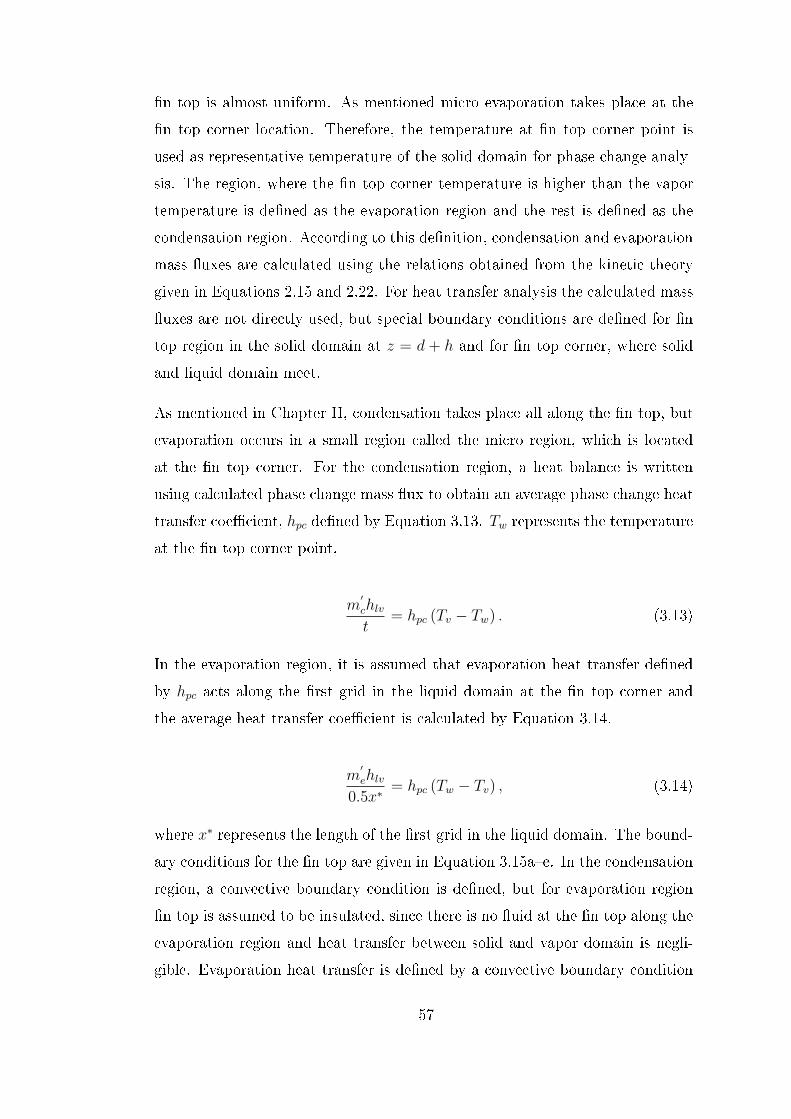
n top is almost uniform. As mentioned micro evaporation takes place at the
n top corner location. Therefore, the temperature at n top corner point is
used as representative temperature of the solid domain for phase change analy-
sis. The region, where the n top corner temperature is higher than the vapor
temperature is dened as the evaporation region and the rest is dened as the
condensation region. According to this denition, condensation and evaporation
mass uxes are calculated using the relations obtained from the kinetic theory
given in Equations 2.15 and 2.22. For heat transfer analysis the calculated mass
uxes are not directly used, but special boundary conditions are dened for n
top region in the solid domain at z = d + h and for n top corner, where solid
and liquid domain meet.
As mentioned in Chapter II, condensation takes place all along the n top, but
evaporation occurs in a small region called the micro region, which is located
at the n top corner. For the condensation region, a heat balance is written
using calculated phase change mass ux to obtain an average phase change heat
transfer coecient, hpc dened by Equation 3.13. Tw represents the temperature
at the n top corner point,
m′chlvt
= hpc (Tv − Tw) . (3.13)
In the evaporation region, it is assumed that evaporation heat transfer dened
by hpc acts along the rst grid in the liquid domain at the n top corner and
the average heat transfer coecient is calculated by Equation 3.14.
m′ehlv
0.5x∗= hpc (Tw − Tv) , (3.14)
where x∗ represents the length of the rst grid in the liquid domain. The bound-
ary conditions for the n top are given in Equation 3.15ac. In the condensation
region, a convective boundary condition is dened, but for evaporation region
n top is assumed to be insulated, since there is no uid at the n top along the
evaporation region and heat transfer between solid and vapor domain is negli-
gible. Evaporation heat transfer is dened by a convective boundary condition
57

only for the n top corner point,
ks∂T
∂z=hpc (Tv − T ) 0 < x < t ; z = d+ h ; T < Tv (3.15a)
∂T
∂z= 0 0 < x < t ; z = d+ h ; T > Tv (3.15b)
ks∂T
∂z=hpc (T − Tv) t < x < t+ x∗ ; z = d+ h ; T > Tv (3.15c)
Equations (3.11) and (3.12) are solved by nite dierence method subject to
the boundary conditions dened by Equations 3.11ad, 3.12ac and 3.15ac.
Liquid domain does not have a pre-determined shape due to the variation of the
liquidvapor interface radius along the heat pipe axis. Therefore, a coordinate
transformation is applied for this region, where the transformed coordinates are
dened as,
λ = x (3.16a)
η = y (3.16b)
ξ = z0
(1 +
z − z04di (y)− z0
4d0)
(3.16c)
where z0 is equal to the groove thickness, 4di is the depth at each x position
along the groove and 4d0 is the depth of the liquid at the center of the chan-
nel x = t. Equation (3.12) can be rewritten using the new coordinates and
rearranging the terms as follows,
u
(∂T
∂η+ a0
∂T
∂ξ
)+ w
(a1∂T
∂ξ
)=
klρCpl
(∂2T
∂λ2+∂2T
∂η2+ a2
∂2T
∂ξ2
)+
klρCpl
(a3∂2T
∂λ∂ξ+ a4
∂2T
∂η∂ξ+ a5
∂T
∂ξ
)+
µ
ρlCplΦ (3.17)
58

where the coecients are dened as,
a0 =∂ξ
∂y(3.17a)
a1 =∂ξ
∂z(3.17b)
a2 =
(∂ξ
∂x
)2
+
(∂ξ
∂y
)2
+
(∂ξ
∂z
)2
(3.17c)
a3 = 2∂ξ
∂x(3.17d)
a4 = 2∂ξ
∂y(3.17e)
a5 =∂2ξ
∂x2+∂2ξ
∂y2+∂2ξ
∂z2(3.17f)
The details about the coordinate transformation are given in Appendix A.
At the solidliquid interface the solution domain includes volumes, half of which
are solid and uniform, where the other half are liquid and non-uniform. For this
region Equations 3.11 and 3.12 cannot be used directly, therefore a heat balance
for each volume is written explicitly. There are four dierent regions (i) Region
I, the interface located at the bottom of the groove, (ii) Region II, the interface
located at the groove bottom corner, and (iii) Region III, the interface located
along the depth of the groove, and (iv) Region IV, the interface located at n
top corner, which are shown in Figure 3.7. The details of the derivation of these
equations are explained in Appendix B.
Due to the skewness of the control volume in Region IV (Figure 3.7) and the
dierence in equations used in the bulk liquid domain and solidliquid interface
domain (Region IIV) and to provide a transition from interface region to the
bulk liquid domain, special equations using overall heat balance equations for
control volumes are written for Region V, which are explained in Appendix B.
59

3.2.1 Grid generation
The rst step in the solution of heat transfer equations given in Equations 3.11,
3.17 and Appendix B is the generation of grid points. There are four subregions
for each x − z plane: (i) Region A, the lower side of the n, (ii) Region B, the
solid domain bottom of the groove, (iii) Region C, upper side of the n, (iv)
Region D, liquid domain in the groove. In each region the grid points are equally
spaced along a constant coordinate line, whose denitions are given in Equations
3.18af. The computational grid structure in the physical domain is presented
in Figure 3.7. The number of grid points in xdirection is m1 for Region A and
C, where m−m1 points are dened in Region B and D. In zdirection k1 points
are used in Region A and B, where the number is k− k1 in Region C and D. In
the axial direction (y) there is no dierence between the four regions, where n
points are dened.
xi =xi−1 +t
m1 − 1(3.18a)
xi =t+
(xi−1 +
b
m−m1
)(3.18b)
yj =yj−1 +L
n− 1(3.18c)
zk =zk−1 +z0
k − 1(3.18d)
zk =zk−1 +z0
k − 1(3.18e)
zk =z0 +
(zk−1 +
(4di)jk − k1
)(3.18f)
60

x,i
z,k
m1 m
k1
k
id
0d
Region I
Region III
Region II
Region IV
D
C
B A
Region V
Figure 3.7: Computational grid in the physical domain at a cross-section of thechannel
3.3 Solution Procedure
Axial momentum equation detailed in Section 3.1 in the liquid domain is coupled
with the heat transfer equation detailed in Section 3.2. As explained in Chapter
II, phase change mass ux equation is a function of n top corner temperature,
solidliquid contact angle, which is related to the liquidvapor interface radius
through the geometry. Momentum equation is coupled to the phase change
mass uxes through the mass balance. The lengths of the evaporation and
condensation regions along the heat pipe axis are unknown at the beginning of
the solution and depend on the n top corner temperature distribution along the
heat pipe axis. All the parameters dening the problem are coupled, therefore
an iterative solution procedure is applied.
The solution procedure starts with the solution of the axial momentum equa-
61

tion (Equation 3.4) for the distribution of liquidvapor interface radius vari-
ation, R(y). The input values are the liquidvapor interface radius, R0, the
liquid velocity, u0, at the beginning of the condensation region and the vapor
temperature, Tv. Mass balance equation (Equation 3.10) is used to nd axial
liquid velocity, u(y), the evaluation of which requires total phase change mass
ow rates, mt. Total phase change mass ow rates consist of evaporation and
condensation mass uxes obtained from micro region relations (Equations 2.15
and 2.22) and from macro or meniscus region. Macro region phase change mass
uxes are calculated from the heat balance written for the liquidvapor interface
region using the temperature distribution in the liquid domain given in appendix
B Section VI. For the rst step of iteration, there is no calculated temperature
distribution, therefore an assumed n top corner temperature distribution along
the heat pipe axis, Tw(y), is used to calculate the micro region phase change
mass ow rates and macro region phase change mass ow rates are not included
in the mass balance. After liquidvapor interface radius variation, R(y), and
liquid velocity, u(y), values are obtained, grid points are generated as dened
in Section 3.2.1 for the heat transfer analysis. The transverse velocity, w, is re-
quired at each grid point for convective terms in Equation 3.17, therefore mass
balance is written for each control volume using the axial velocity distribution
and phase change mass ow rates.
mi − mo + mby − mbz − mty + mtz = 0 (3.19)
where
mi =1
2(uj−1 + uj) ρlAy
j− 12
(3.19a)
mo =1
2(uj+1 + uj) ρlAy
j+12
(3.19b)
mby = ujρlAbny (3.19c)
62

mty = ujρlAtny (3.19d)
Ay represents the cross-sectional area in the x−z plane and u(j) axial velocity in
each y−position. Since the areas are dierent on each face due to the irregular
shape of the liquid domain, they are approximated as trapezoidal areas and
calculated for each control volume using the solution domain grid points. The
upper and lower surfaces of the liquid control volumes are curved due to the
axial variation of interface radius and the surface normal has components in the
x and ycoordinates. The area Anty represents the projected area of the upper
curved surface on the x-z plane, which is also approximated as a trapezoidal
area and calculated using grid points. Anby is the projected area of the lower
curved surface. Figure 3.8 shows the mass ows into and out of the control
volumes at a constant x−line on the y − z plane. The calculation starts from
the bottom control volumes at the solidliquid interface and the calculated mtz
values are equated to mbz of the upper grid point. Since the grid points are
dened centrally in the control volumes, average of mbz and mtz values are used
in the calculation of the velocity w(x, y, z).
63

i,j,k
y
z
Figure 3.8: Mass balance in the liquid domain for the calculation of transversevelocity
Heat transfer equations Equation 3.11, 3.17 and heat balance equations given in
Appendix B Section IV are solved subject to the boundary conditions 3.11ad,
3.12ac and 3.15ac. Since the newly obtained temperature distribution is dier-
ent than the initial n top corner temperature, Tw(y), a successive substitution
procedure is applied for Tw until convergence is reached. During temperature
iterations, phase change mass ow rates from micro regions are also recalculated
using new values of the n top corner temperatures. At the end of the analysis
the overall evaporated mass should be equal to condensed mass, which implicitly
satises overall energy balance of the solution domain. Therefore, evaporation
and condensation mass uxes from macro regions are calculated using the con-
verged temperature distribution and the mass uxes are calculated from the
energy balance written for the liquidvapor interface or top of the liquid do-
main region (Appendix B, Section VI). Micro and macro region mass uxes are
integrated along the y−axis and sum of the evaporated and condensed masses
are found, which are not equal until convergence. The vapor temperature is a
64

parameter dening the phase change mass uxes, therefore an iteration using
the secant method is carried out to equalize the masses in terms of vapor tem-
perature, Tv. During these iterations micro region phase change mass uxes are
recalculated for new values of vapor temperature, Tv, in each iteration, which is
terminated, when a set convergence criteria is satised.
At this point, the liquidvapor interface radius variation, R(y), and temperature
distribution in the solid and liquid domains are not compatible, since phase
change mass uxes from micro regions are recalculated during iterations for
new values of vapor temperature, Tv, and n top corner temperature, Tw(y).
Therefore, the solution of axial momentum equation is repeated for new values
of Tv, Tw(y) and mass ow rates from macro region. This iteration procedure is
repeated until the change in Tv satises a set convergence criteria. The solution
procedure is summarized in Figure 3.9.
65

Iteration for Tv
Solve momentum
equation for R(y)
Solve heat transfer
equation for Tw
Iteration for Tw
Check
oldw
neww TT
criterion
Iteration phase change
mass balance
Check
cmacroemicroe
cmacroemicroe
mmm
mmm
,,
,, /
Check
oldv
newv TT
criterion
criterion
Finish
NO
NO
NO
Figure 3.9: Flowchart for the solution procedure
66

CHAPTER 4
RESULTS FOR HEAT PIPE MODEL
In this chapter the results obtained for the heat pipe model will be compared
with those available in the literature. In the second part a sample problem
is introduced and the eect of the physical and thermal parameters will be
investigated for a constant heat input. The axial variation of the temperature
and liquidvapor interface will be provided to understand the eect of various
parameters on heat pipe performance. The last part includes the study of the
maximum heat capacity of the heat pipe in terms of dierent groove width,
groove depth combinations, where at the end of the evaporation region dry-out
limit is reached.
4.1 Validation of the Present Study
The results of the present study are compared to the experimental/numerical
study of Lefevre et al. [6] for validation. The at heat pipe used in the study
is made of copper and the working uid is methanol. The physical properties
used in the computations are given in Table 4.1
67

Table 4.1: Dimension and physical properties used in validation model
Channel length mm 230
Groove width mm 0.2
Fin thickness mm 0.2
Groove thickness mm 2
Groove depth mm 0.38
Length of heat source region mm 190
Length of heat sink region mm 30
Thermal conductivity of solid W/m·K 400
Thermal conductivity of liquid W/m·K 0.2
Latent heat of evaporation kJ/kg 1085
Density of liquid kg/m3 792
Dynamic viscosity of liquid Pa·s 3.14× 10⁻⁴
Specic heat of liquid J/kg·K 2530
Surface tension N/m 18.5× 10⁻³
Molar mass of liquid kg/mol 32× 10−3
Molar volume of liquid m3/mol 42× 10−6
Vapor pressure Pa 1.31× 10⁵
Heat load W/m2·K 5000
Ambient heat transfer coecient W/m2·K 2100
Ambient temperature K 323
Two parameters are used to analyze and compare the results. The rst one
is the liquidvapor interface radius variation along the heat pipe axis, which
generates the driving capillary pressure. The second one is the temperature at
n top corner point where solidliquidvapor domains meet, which is used as a
representative temperature of the heat pipe. The temperature at this location
will be termed as the edge temperature. The results for the interface radius
variation is given in Figure 4.1. The dierence between the present study and
the results of [6] is within 9% when convective heat transfer in the liquid domain
68

is not included. There is no considerable dierence in the results when eect of
convection is included.
0.0E+00
2.0E-04
4.0E-04
6.0E-04
8.0E-04
1.0E-03
1.2E-03
1.4E-03
0 0.05 0.1 0.15 0.2 0.25
Axial position (m)
Inte
rfa
ce
ra
diu
s (
m)
Results of Lefevre et al
Present study (w/o convection)
Present study (convection)
Figure 4.1: Liquid interface radius variation along the heat pipe axis
The variation of liquid velocity, u(y), along the heat pipe axis is given in Fig-
ure 4.2. At the beginning of the condensation region the liquid velocity is zero
and increases to a maximum value of 5.3 mm/s at the end of the condensation
region, 4.4 cm away from the beginning of the groove. The axial liquid veloc-
ity starts to decrease due to evaporation in spite of the decrease in the liquid
cross-sectional area until the end of the heat pipe axis.
69

0.0E+00
1.0E-03
2.0E-03
3.0E-03
4.0E-03
5.0E-03
6.0E-03
0 0.05 0.1 0.15 0.2 0.25
Axial position (m)
Liq
uid
Velo
cit
y (
m/s
)
Figure 4.2: Axial liquid velocity variation along the heat pipe axis
338
339
340
341
342
343
344
345
346
0 0.05 0.1 0.15 0.2 0.25
Axial position (m)
Ed
ge t
em
pera
ture
(K
)
Results of Lefevre et al
Present study (w/o convection)
Present study (convection)
Figure 4.3: Edge temperature variation along the heat pipe axis
The edge temperature variation is given in Figure 4.3, where the dierence
between the present study and Lefevre et al. [6] is about 2 K for both with and
70

without liquid convection eect, where the maximum value of the dierence is
located in the evaporation region. Vapor temperature is given as 343 K in [6],
where the corresponding values are 342.86 K and 342.83 K for the present study
without liquid convection eect and including liquid convection, respectively.
The temperature distribution in the solid and liquid domains is shown in Figure
4.4. The axial temperature variation is dominant and the transverse temperature
distribution in the solid domain is almost uniform due to the high thermal
conductivity of the solid and high value of heat pipe length to depth ratio.
Figure 4.4: 3-D temperature distribution in the liquid and solid regions
As seen in Figure 4.3, there are two discrepancies in the edge temperature be-
tween the present study and [6], which are the temperature dierences in magni-
tude for both in the condensation and evaporation regions and the temperature
gradient in the condensation region. This condition can be the result of the ther-
mal modeling used in the two studies. An electrical analogy is used to model
the heat transfer along the heat pipe axis in [6]. Each crosssection of the heat
71

pipe was modeled separately, which in turn, was used to calculate the thermal
resistance in the transverse direction. Conduction in solid domain was used to
obtain the longitudinal resistance. The approach used in thermal modeling for
heat source and sink regions are similar, where a constant heat ux was applied
along the heat source region and convection boundary condition was dened for
the heat sink region. At the liquidvapor interface a convective boundary con-
dition was dened, where the phase change heat transfer coecient was dened
from the formula derived from kinetic theory. Similar to the present study the
liquid lm distribution along the n top was obtained for the condensation re-
gion and conduction through the liquid lm was considered. For the evaporation
region n top surface was taken adiabatic. In [6], phase change heat transfer
coecient was a function of vapor saturation temperature and pressure, which
were constant along the heat pipe axis. Therefore, a constant phase change heat
transfer coecient was used at the liquidvapor interface for both the evapo-
ration and condensation regions. However, in the present study phase change
mass uxes are calculated directly from kinetic theory rendering them functions
of the edge temperature and the solidliquid contact angle, which change along
the heat pipe axis.
In the present study, evaporation from micro and macro regions are considered
separately, where in [6] a constant phase change heat transfer coecient was
dened along the liquidvapor interface. It is seen that coupling of micro region
evaporation heat ux for the n top corner point has a large impact on the
temperature distribution along the heat pipe. In the micro region, whose length
is about 1 micrometer, evaporation heat ux is obtained and it is distributed
along the rst control volume in the liquid phase by dening an average phase
change heat transfer coecient, whose value is approximately 12 orders of
magnitude lower than the value calculated from the formula given in [6]. If the
formula given in [6] is applied along the liquidvapor interface, the temperature
distribution at each cross-section on the x − z plane becomes more uniform
and closer to the vapor temperature. For the condensation region the model
used in the present study depends also on the contact angle which decreases
along the heat pipe axis. As mentioned in Chapter II, condensation mass ux
72

decreases with decreasing contact angle. At the beginning of the condensation
region, the condensation mass ux is high and solid wall temperature should be
lower to increase the convective heat transfer to the ambient, which results in a
temperature gradient in the condensation region.
One of the advantages of heat pipes is the reduction of the temperature dierence
between the heat source and heat sink regions. Same amount of heat input used
in the validation study is transferred by a copper block, where the axial edge
temperature variation is given in Figure 4.5. As shown in the gure the axial
temperature dierence increases to 138 K, whereas the corresponding dierence
is 7 K in the heat pipe. The heat pipe solution shows that 86% of the input heat
load is transferred by phase change through the heat pipe. Therefore, by causing
an approximately constant temperature region on the evaporation region, phase
change results in a steeper temperature gradient in the solid, thus eectively
increasing the conduction heat transfer in the solid. As a result eectively 15%
of the heat input is transferred through one third of the heat pipe length by
conduction, which results in 138 K temperature dierence, which is consistent
with the result given in Figure 4.5.
73

338
339
340
341
342
343
344
345
346
347
0 0.05 0.1 0.15 0.2
Axial position (m)
Co
rner
tem
pera
ture
(K
)
300
320
340
360
380
400
420
440
460
480
500
Wall
Tem
pera
ture
(K
)
Heat Pipe Solution
Equivalent Copper Block
Figure 4.5: Edge temperature variation in the heat pipe and copper block
4.2 A Parametric Study of Heat Pipe Performance
A parametric study is conducted to understand the eect of parameters such
as heat load, ambient heat transfer coecient, the radius at the beginning of
the condensation region, groove depth and width, n thickness, the length of
heat sink and source region on the liquidvapor interface radius and the edge
temperature variation for the same amount of heat input. In this case the
working uid and heat pipe material are the same as in the validation study,
i.e. methanol and copper. The dimensions of the groove are dierent as given
in Table 4.2. In this case the heat source region is shorter than the heat sink
region. A sample problem is introduced to simulate the cooling of an electronic
device on a circuit board. It is seen that heat dissipation rates of CPU's range
from 20100 W, where the size of the device is approximately 50 mm × 50 mm.
Therefore in the parametric study, a heat load of 50 W is applied on a heat
source region of 50 mm × 50 mm dimension. The heat transfer coecient with
74

the ambient heat transfer coecient is taken as 250 W/m2·K, which is typically
in the range of forced convection heat transfer. The ambient temperature is set
at 50C, which is a typical dened maximum operating ambient temperature for
electronic components. The case dened in this section is taken as a baseline
and the eect of the change in the parameters are explained in the following
sections.
Table 4.2: Dimension and physical properties used in theparametric study
Channel length mm 200
Groove width mm 0.2
Fin thickness mm 0.2
Groove thickness mm 2
Groove depth mm 0.4
Length of heat source region mm 50
Length of heat sink region mm 150
Thermal conductivity of solid W/m·K 400
Thermal conductivity of liquid W/m·K 0.2
Latent heat of evaporation kJ/kg 1085
Density of liquid kg/m3 792
Dynamic viscosity of liquid Pa·s 3.14× 10⁻⁴
Specic heat of liquid J/kg·K 2530
Surface tension N/m 18.5× 10⁻³
Molar mass of liquid kg/mol 32× 10−3
Molar volume of liquid m3/mol 42× 10−6
Vapor pressure Pa 1.31× 10⁵
Heat load W/m2 20000
Ambient heat transfer coecient W/m2·K 250
Ambient temperature K 323
75

4.2.1 The eect of ambient heat transfer coecient
Ambient heat transfer coecient for the baseline case is 250W/m2·K as given in
Table 4.2. This value is increased and decreased by 50%. As given in Figure 4.5,
the change in ambient heat transfer coecient has no considerable eect on the
interface radius variation. Since the heat load is constant in all three cases, there
is an equal amount of heat input for evaporation, which is the driving force for
the heat transfer problem. The iterative process is terminated when the evap-
oration and condensation mass uxes equalize in terms of vapor temperature.
Higher vapor temperatures and consequently higher edge temperatures (Figure
4.7) are obtained for lower heat transfer coecients. The analysis is performed
to show that operating range of the heat pipe can be adjusted by changing the
amount of cooling at the heat sink region.
0.0E+00
2.0E-04
4.0E-04
6.0E-04
8.0E-04
1.0E-03
1.2E-03
1.4E-03
0 0.02 0.04 0.06 0.08 0.1 0.12 0.14 0.16 0.18 0.2
Axial position (m)
Inte
rface r
ad
ius (
m)
Baseline
150% of baseline
50% of baseline
Figure 4.6: Liquid interface radius variation along the heat pipe axis for dierentambient heat transfer coecients
76

320
330
340
350
360
370
380
390
0 0.02 0.04 0.06 0.08 0.1 0.12 0.14 0.16 0.18 0.2
Axial position (m)
Ed
ge t
em
pera
ture
(K
)
Baseline, Tv = 350.6K
150% of baseline, Tv = 341.6K
50% of baseline, Tv = 377.8K
Figure 4.7: Edge temperature variation along the heat pipe axis for dierentambient heat transfer coecients
4.2.2 The eect of solid thermal conductivity
Copper container is used for the baseline analysis whose thermal conductivity is
400 W/m·K. The eect of the thermal conductivity is investigated by reducing
the value to 25 W/m·K, which is in the range of that of stainless steel. The
variation of the liquid interface radius shows a similar behavior for the two cases
(Figure 4.8), where input heat load is identical and consequently so is the evap-
oration heat transfer. For decreasing thermal conductivity of the container, the
contribution of the axial heat transfer decreases and the amount of heat transfer
used for phase change increases, which can be seen in the ratio of the heat trans-
ferred via phase change to the input heat load is 81% for the baseline copper
case, which increases to 98% with low solid thermal conductivity. Some previous
studies which did not consider axial heat transfer assumed that evapora-
tion and condensation regions are constrained with heat source and heat sink
regions. However, axial heat transfer causes a smooth transition from condensa-
tion to evaporation regions as shown in Figure 4.9. As the thermal conductivity
77
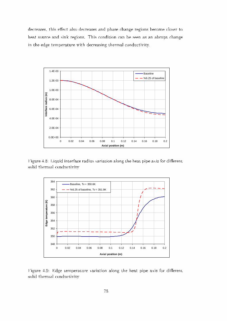
decreases, this eect also decreases and phase change regions become closer to
heat source and sink regions. This condition can be seen as an abrupt change
in the edge temperature with decreasing thermal conductivity.
0.0E+00
2.0E-04
4.0E-04
6.0E-04
8.0E-04
1.0E-03
1.2E-03
1.4E-03
0 0.02 0.04 0.06 0.08 0.1 0.12 0.14 0.16 0.18 0.2
Axial position (m)
Inte
rface r
ad
ius (
m)
Baseline
%6.25 of baseline
Figure 4.8: Liquid interface radius variation along the heat pipe axis for dierentsolid thermal conductivity
348
350
352
354
356
358
360
362
364
0 0.02 0.04 0.06 0.08 0.1 0.12 0.14 0.16 0.18 0.2
Axial position (m)
Ed
ge t
em
pera
ture
(K
)
Baseline, Tv = 350.6K
%6.25 of baseline, Tv = 351.9K
Figure 4.9: Edge temperature variation along the heat pipe axis for dierentsolid thermal conductivity
78

4.2.3 The eect of heat load
Initial heat ux value, 20kW/m2, is decreased by 20% and 40% and increased
by 20% to investigate the eect of the input heat load. As expected, higher
heat loads result in more evaporation and smaller radius is obtained for the
evaporation region (Figure 4.10). More evaporation leads to higher temperature
dierences at the heat sink region, since the same amount of uid should con-
densate to satisfy the overall mass balance. Therefore, the vapor temperature
(Tv) also increases with increasing heat load. As expected, more uid should be
present for higher heat input, which is shown in Figure 4.12.
0.0E+00
2.0E-04
4.0E-04
6.0E-04
8.0E-04
1.0E-03
1.2E-03
1.4E-03
0 0.02 0.04 0.06 0.08 0.1 0.12 0.14 0.16 0.18 0.2
Axial position (m)
Inte
rface r
ad
ius (
m)
Baseline
120% of baseline
80% of baseline
60% of baseline
Figure 4.10: Liquid interface radius variation along the heat pipe axis for dier-ent heat load values
79

335
340
345
350
355
360
365
370
0 0.02 0.04 0.06 0.08 0.1 0.12 0.14 0.16 0.18 0.2
Axial position (m)
Ed
ge t
em
pera
ture
(K
)
Baseline
120% of baseline
80% of baseline
60% of baseline
Figure 4.11: Edge temperature variation along the heat pipe axis for dierentheat load values
338
340
342
344
346
348
350
352
354
356
358
10000 12000 14000 16000 18000 20000 22000 24000 26000
Heat flux (W/m2 K)
Vap
or
tem
pera
ture
(K
)
3.05E-05
3.10E-05
3.15E-05
3.20E-05
3.25E-05
3.30E-05
3.35E-05
To
tal
flu
id m
ass (
kg
)
Vapor temperature (K)
Total fluid mass(kg)
Figure 4.12: Vapor temperature and total uid mass variation for dierent heatload values
80

4.2.4 The eect of initial interface radius
The initial radius is 1200 micrometers for baseline study, which is reduced by
50% and increased by 50% and 200%. The eect of initial interface radius
on the variation of the interface radius along the heat pipe is given in Figure
4.13. When the initial radius increases, the change along the heat pipe axis
increases, the change is %44 for the case when the initial radius is only 50% of
the baseline case; and it increases to 67% when the initial radius is 150% of the
baseline case. As mentioned in Chapter II, contact angle is a parameter for phase
change modeling. When the interface radius decreases, contact angle decreases,
which results in lower condensation but higher evaporation mass uxes. As the
interface radius decreases heat transfer rate for condensation decreases from 0.25
W to 0.23 W. However, heat transfer rate for micro region evaporation increases
from 0.06 W to 0.08 W. Therefore, approximately the same amount of heat load
is used for phase change, which is about 81% of the heat input. Consequently the
change in the edge temperature is not considerable and there is approximately 1
K dierence, which can be seen in Figure 4.14 and there is approximately 0.8 K
change in the vapor temperature as shown in Figure 4.15. It is expected that
increasing initial radius will increase the amount of uid mass. However, with
increasing initial radius the uid mass in the heat pipe decreases as shown in
Figure 4.15. This eect can be explained by the condensed mass on the n top,
since smaller radii result in steeper variation of the liquid lm thickness on the
n top as explained in Chapter II Figure 2.9. The integration of the liquid lm
thickness to calculate the liquid volume on the n top gives higher values for
steeper lm thickness variation, which increases overall uid mass in the heat
pipe, even the uid mass inside the groove decreases with decreasing radius.
81

0.0E+00
5.0E-04
1.0E-03
1.5E-03
2.0E-03
2.5E-03
3.0E-03
0 0.02 0.04 0.06 0.08 0.1 0.12 0.14 0.16 0.18 0.2
Axial position (m)
Inte
rface r
ad
ius (
m)
Baseline
50% of baseline
150% of baseline
200% of baseline
Figure 4.13: Liquid interface radius variation along the heat pipe axis for dier-ent initial radius values
348
350
352
354
356
358
360
362
0 0.02 0.04 0.06 0.08 0.1 0.12 0.14 0.16 0.18 0.2
Axial position (m)
Ed
ge t
em
pera
ture
(K
)
Baseline
50% of baseline
150% of baseline
200% of baseline
Figure 4.14: Edge temperature variation along the heat pipe axis for dierentinitial radius values
82

350.2
350.3
350.4
350.5
350.6
350.7
350.8
350.9
351.0
351.1
351.2
0.5 1.0 1.5 2.0 2.5 3.0 3.5 4.0 4.5 5.0
Initial radius (mm)
Vap
or
tem
pera
ture
(K
)
0.0E+00
5.0E-06
1.0E-05
1.5E-05
2.0E-05
2.5E-05
3.0E-05
3.5E-05
4.0E-05
To
tal
flu
id m
ass (
kg
)
Vapor temperature
total fluid mass
Figure 4.15: Vapor temperature and uid mass for dierent initial radius values
4.2.5 The eect of groove depth
Three dierent groove depth values are investigated, which are 300, 400 and 500
micrometers, where the depth is 400 micrometers for the baseline study. When
the depth is larger, the amount of uid in the heat pipe increases, which gen-
erates a larger thermal resistance. Fluid masses in the heat pipe vary between
2.86×10⁻⁵kg, 3.24×10⁻⁵ kg, 3.78×10⁻⁵kg from 300 to 500 micrometers groove
depths, respectively. The ratio of the heat load for phase change to input heat
load increases with decreasing groove depth, whose change is about 2% for this
case. As a result, the interface radius is smaller for the 75% of the baseline
case (Figure 4.16). However, the edge temperature variation gives almost same
distribution for all three cases (Figure 4.17). Although, with increasing groove
depths phase change heat transfer from micro region decreases, a larger propor-
tion of the heat load is conducted through the liquid and used in the macro
region evaporation. These two eects can be the reason for the approximately
constant edge temperature and consequently vapor temperature (Figure 4.17),
83

which is approximately 350.7 K.
0.0E+00
2.0E-04
4.0E-04
6.0E-04
8.0E-04
1.0E-03
1.2E-03
1.4E-03
0 0.02 0.04 0.06 0.08 0.1 0.12 0.14 0.16 0.18 0.2
Axial position (m)
Inte
rface r
ad
ius (
m)
Baseline
75% of baseline
125% of baseline
Figure 4.16: Liquid interface radius variation along the heat pipe axis for dier-ent groove depths
348
350
352
354
356
358
360
362
0 0.02 0.04 0.06 0.08 0.1 0.12 0.14 0.16 0.18 0.2
Axial position (m)
Ed
ge t
em
pera
ture
(K
)
Baseline
75% of baseline
125% of baseline
Figure 4.17: Edge temperature variation along the heat pipe axis for dierentgroove depths
84

4.2.6 The eect of n thickness
The eect of n thickness is investigated without changing the groove width,
where the n thicknesses are 400, 200 and 100 micrometers, where the 200
micrometers is used in the baseline study. As given by Zhang and Faghri [52] a
decrease in n thickness results in a thinner condensation layer on the n top,
which causes higher heat ux values and overall heat transfer depends on the
integration of the ux values along the n top. For the present case, increasing
n thickness results in an increase in the condensation heat transfer rate, which
results in an increase in the evaporation heat transfer rate since the overall energy
balance should be satised at the end of the solution procedure. The eect can
be seen in the interface radius variation given in Figure 4.18. The interface
radius for the n thickness of 400 micrometers has the smallest value at the end
of the heat pipe axis. Since the condensate mass on the n top increases with
increasing thickness, total uid mass in the heat pipe has the largest value at 400
micrometers, where the values are 6.34×10⁻⁵kg, 3.24×10⁻⁵ kg and 2.62×10⁻⁵kg
for 400, 200 and 100 micrometers, respectively. Changing n thickness does not
aect the edge temperature in the condensation region, whereas the temperature
in the evaporation region has higher values for increased n thickness (Figure
4.19). The result is compatible with increased evaporation heat transfer for
larger n thicknesses.
85

0.0E+00
2.0E-04
4.0E-04
6.0E-04
8.0E-04
1.0E-03
1.2E-03
1.4E-03
0 0.02 0.04 0.06 0.08 0.1 0.12 0.14 0.16 0.18 0.2
Axial position (m)
Inte
rfa
ce
ra
diu
s (
m)
Baseline
50% of baseline
200% of baseline
Figure 4.18: Liquid interface radius variation along the heat pipe axis for dier-ent n thickness
348
350
352
354
356
358
360
362
364
0 0.02 0.04 0.06 0.08 0.1 0.12 0.14 0.16 0.18 0.2
Axial position (m)
Ed
ge t
em
pera
ture
(K
)
Baseline
50% of baseline
200% of baseline
Figure 4.19: Edge temperature variation along the heat pipe axis for dierentn thickness
86

4.2.7 The eect of groove width
For this section the eect of the groove width is investigated, where the groove
widths are 400, 200 and 100 micrometers, where 200 micrometers is used for the
baseline study. The uid mass inside the heat pipe is 5.58× 10⁻⁵kg, 3.24× 10⁻⁵
kg, 2.44 × 10⁻⁵kg for 400, 200 and 100 micrometers, respectively. Since by
decreasing the groove width, the uid mass inside the heat pipe decreases, a
larger portion of the heat load is used for phase change. The ratios of the phase
change heat transfer to the input heat load are 86%, 81% and 76% for 100, 200
and 400 micrometers groove widths, respectively. Due to increase in the phase
change heat transfer for smaller grooves, the interface radius for 100 micrometers
groove width gets the smallest value at the end of the heat pipe axis (Figure
4.20). The edge temperature variation is given in Figure 4.21, where dierent
values of groove widths only aect the temperature in the evaporation region.
0.0E+00
2.0E-04
4.0E-04
6.0E-04
8.0E-04
1.0E-03
1.2E-03
1.4E-03
0 0.02 0.04 0.06 0.08 0.1 0.12 0.14 0.16 0.18 0.2
Axial position (m)
Inte
rface r
ad
ius (
m)
Baseline
50% of baseline
200% of baseline
Figure 4.20: Liquid interface radius variation along the heat pipe axis for dier-ent groove width
87

348
350
352
354
356
358
360
362
364
366
0 0.02 0.04 0.06 0.08 0.1 0.12 0.14 0.16 0.18 0.2
Axial position (m)
Ed
ge t
em
pera
ture
(K
)
Baseline
50% of baseline
200% of baseline
Figure 4.21: Edge temperature variation along the heat pipe axis for dierentgroove width
4.2.8 The eect of working uid
Thermophysical properties of the working uids dene phase change character-
istics and operational range of the heat pipe. To show this eect three dierent
working uids compatible with copper container are analyzed. The physical
properties are given in Table 4.3. Latent heat of evaporation of methanol, which
is the baseline for this study, is about half of that of water, therefore there is
more evaporating mass in the case of methanol, whose eect can be seen in the
interface radius variation given in Figure 4.22. It is expected that evaporated
mass of ammonia becomes larger than methanol, since the latent heat of am-
monia is lower than that of methanol. The heat ow rate used for evaporation
is 0.35 W for ammonia and 0.32 W for methanol and this dierence does not
result in a considerable dierence in the interface radius.
88

Table 4.3: Thermophysical properties of working uids
Methanol Water Ammonia
Thermal conductivity W/m·K 0.2 0.67 0.36
Latent heat of evaporation kJ/kg 1085 2308 895
Density kg/m3 792 972 512
Dynamic viscosity Pa·s 3.14× 10⁻⁴ 3.51× 10⁻⁴ 8.32×10⁻⁵
Surface tension N/m 18.51×10⁻³ 62.69×10⁻³ 9.6× 10⁻³
Molar mass kg/mol 32× 10−3 18× 10−3 17× 10−3
Molar volume m3/mol 42× 10−6 18× 10−6 33× 10−6
Specic heat J/kg·K 2530 4197 5639
Vapor Pressure Pa 1.31× 10⁵ 0.47× 10⁵ 3.86× 10⁶
Thermal conductivity of the working uid aects heat transfer in the liquid do-
main and temperature distribution along the heat pipe wall. Higher thermal
conductivity values, as given for water here, result in a lower temperature dier-
ence between the evaporation and condensation region, which is 5 K for water
and 10 K for methanol (Figure 4.23). This behavior can be also seen for am-
monia, the temperature dierence between the evaporation and condensation
regions is reduced to 6 K.
89

0.0E+00
2.0E-04
4.0E-04
6.0E-04
8.0E-04
1.0E-03
1.2E-03
1.4E-03
0 0.02 0.04 0.06 0.08 0.1 0.12 0.14 0.16 0.18 0.2
Axial position (m)
Inte
rface r
ad
ius (
m)
Baseline
Ammonia
Water
Figure 4.22: Liquid interface radius variation along the heat pipe axis for dier-ent working uids
348
350
352
354
356
358
360
362
0 0.02 0.04 0.06 0.08 0.1 0.12 0.14 0.16 0.18 0.2
Axial position (m)
Ed
ge t
em
pera
ture
(K
)
Baseline
Ammonia
Water
Figure 4.23: Edge temperature variation along the heat pipe axis for dierentworking uids
90

4.2.9 The eect of heat source and sink region length
The eect of dierent heat source and heat sink lengths are studied in this
section for the same total heat input. The cases are summarized in Table 4.4.
Addition of an adiabatic region between the two ends increases the eectiveness
of the heat pipe, where the ratio of phase change heat transfer to the heat input
is 81% for baseline case, the ratio increases to 97% for a 50mm adiabatic region
and 99% for a 75mm adiabatic region. The 150 mm heat source case is similar
to the validation problem. For this case the interface radius is smaller at the
end of the evaporation region compared to the baseline case, but it is larger
than the cases with adiabatic regions as shown in Figure 4.24. The advantage
of this case is the reduction in temperature dierence between the evaporator
and condenser sides, which is 6 K as opposed to the baseline 10 K dierence
(Figure 4.25). However, the ratio of phase change heat transfer to input heat is
84% and smaller than the cases with adiabatic regions.
Table 4.4: Dimensions of heat source, heat sink and adiabatic regions
Heat Adiabatic Heat
Source Region Sink
Length Length Length
(mm) (mm) (mm)
Baseline 50 150
50mm adiabatic region 50 50 100
75mm adiabatic region 50 75 25
150mm heat source region 150 50
As seen in Figure 4.25, the lengths of evaporation and condensation regions
change according to the boundary conditions, which are the lengths of the heat
source and heat sink in this case. In the heat pipe, there is a smooth transition
91

from condensation to evaporation region due to axial heat transfer and there is no
denite adiabatic region in the heat pipe, eventhough at the external boundary
a region with an adiabatic boundary condition is dened.
0.0E+00
2.0E-04
4.0E-04
6.0E-04
8.0E-04
1.0E-03
1.2E-03
1.4E-03
0 0.02 0.04 0.06 0.08 0.1 0.12 0.14 0.16 0.18 0.2
Axial position (m)
Inte
rface r
ad
ius (
m)
Baseline
50mm adiabatic region
75mm adiabatic region
150mm heat source
Figure 4.24: Liquid interface radius variation along the heat pipe axis for dier-ent heat sink and source lengths
340
350
360
370
380
390
400
410
420
430
440
0 0.02 0.04 0.06 0.08 0.1 0.12 0.14 0.16 0.18 0.2
Axial position (m)
Ed
ge t
em
pera
ture
(K
)
Baseline
50mm adiabatic region
75mm adiabatic region
150mm heat source
Figure 4.25: Edge temperature variation along the heat pipe axis for dierentheat sink and source lengths
92

4.3 Maximum Heat Capacity of the Heat Pipe
In section 4.2, a constant amount of heat load is applied and the eect of geo-
metric and physical parameters on the interface radius and the edge temperature
is studied. In this section the maximum heat capacity of the heat pipe is investi-
gated. Since for the present model, the analysis for axial momentum starts from
the condensation region and ends at the evaporation region, it is not possible to
nd the minimum interface radius at the end of the evaporation region directly.
However, minimum radius can be dened by the geometry and solidliquid con-
tact angle, which is unique for a specic heat pipe material and working uid
combination,
Rmin =b
cos θ(4.1)
The contact angle is approximately 40 degrees for coppermethanol combination
[6]. Therefore, the input heat load is increased gradually to obtain 40 degrees
at the end of the evaporation region, when dry-out conditions starts to prevail.
4.3.1 Fixed total length of n thickness and groove width
For this analysis the baseline case has the same geometry and boundary con-
ditions used in Section 4.2. Total length of the n thickness and groove width
is 400 micrometers, which is kept constant. Dierent values of groove width
to n thickness ratios are analyzed. Since the total length is constant, number
of grooves is xed for a given heat pipe size. The variation for the maximum
heat ux and vapor temperature is given Figure 4.26. Maximum heat ux in-
creases where the width to thickness ratio reaches the value of three and further
increase in the ratio does not change the maximum heat transfer value, where
similar behavior can be seen in the vapor temperature variation. Evaporation
heat transfer rate from micro region increases until the ratio reaches the value of
three, but then it starts to decrease. On the other hand, the heat transfer rate
from macro evaporation continues to increase, which compensates the increasing
93

value of the condensation heat transfer rate. The ratio of the phase change heat
transfer to the input heat load is almost constant, where the value is 81% for
this section.
0.0E+00
1.0E+04
2.0E+04
3.0E+04
4.0E+04
5.0E+04
6.0E+04
7.0E+04
0.5 1 1.5 2 2.5 3 3.5 4
Groove width/fin thickness
Maxim
um
heat
flu
x (
W /
m2)
360
365
370
375
380
385
390
395
400
405
410
Vap
or
tem
pera
ture
(K
)
Maximum Heat Flux
Vapor Temperature
Figure 4.26: Maximum heat ux and the vapor temperature variation for dier-ent groove width to n thickness ratios
The variation of the total uid mass in the heat pipe is given in Figure 4.27.
The overall uid mass decreases until the ratio reaches the value of two and after
that value it starts to increase. Total uid mass includes the uid in the groove
and the condensate mass on the n top. Increasing groove width also causes an
increase in the uid mass in the groove, however, the condensate mass on the
n top decreases. After the groove width to n thickness ratio reaches the value
of two, the increase in the groove mass dominates and the overall eect can be
seen as an increase in the uid mass. The ratio of the total uid volume to
the groove volume is also given in Figure 4.27, where increasing groove volume
determines the behavior and a continued decrease in the volume ratio can be
seen.
94

3.6E-05
3.7E-05
3.8E-05
3.9E-05
4.0E-05
4.1E-05
4.2E-05
0.5 1 1.5 2 2.5 3 3.5 4
Groove width/fin thickness
To
tal
flu
id m
ass (
kg
)
0
0.5
1
1.5
2
2.5
3
Flu
id v
olu
me/g
roo
ve v
olu
me
Fluid mass
Total volume/groove volume
Figure 4.27: Fluid mass for dierent groove width to n thickness ratios
4.3.2 Eect of dierent groove width and depth for xed n thickness
In the second case, groove width and depth values are changed, where the n
thickness is taken as a constant of 200 micrometers. Groove width varies from
150 to 400 micrometers and the groove depth range is 250 to 600 micrometers.
Maximum heat ux variation for dierent groove width and depth combinations
are shown in Figures 4.284.30. The initial value of the liquid interface radius
is also varied between 0.9 to 2.4 mm. As given in Figures 4.284.30 for a xed
groove width (solid lines), the increase in groove depth causes an increase in
the maximum heat ux values. For a xed groove depth value (dash lines)
an increase in groove width causes an increase in the maximum heat ux to a
peak value after which the maximum heat ux starts to decrease again. As the
groove width increases, evaporation heat transfer from micro region decreases,
whereas evaporation from macro region continues to increase and compensate
condensation. After a certain value, heat transfer from macro region also starts
to decrease. The decreasing ratio of the phase change heat transfer rate to the
95

input heat load also supports this behavior.
1.00
1.10
1.20
1.30
1.40
1.50
1.60
1.70
1.80
1.90
2.00
2.10
2.20
4.0 14.0 24.0 34.0 44.0 54.0 64.0 74.0 84.0
Heat flux x103( W/m2)
Flu
id v
olu
me/g
roo
ve v
olu
me
Depth:250 Depth:300
Depth:400 Depth:500
Depth:600 Width:150
Width:200 Width:250
Width:300 Width:350
Width:400
Figure 4.28: Maximum heat ux variation for dierent groove depths and widthsfor an initial radius of 0.9 mm.
96

1.00
1.10
1.20
1.30
1.40
1.50
1.60
1.70
1.80
1.90
2.00
2.10
8.0 18.0 28.0 38.0 48.0 58.0 68.0 78.0 88.0 98.0 108.0
Heat flux x103(W/m2)
Flu
id v
olu
me
/gro
ov
e v
olu
me
Depth:250 Depth:300
Depth:400 Depth:500
Depth:600 Width:150
Width:200 Width:250
Width:300 Width:350
Width:400
Figure 4.29: Maximum heat ux variation for dierent groove depths and widthsfor an initial radius of 1.2 mm.
1.00
1.10
1.20
1.30
1.40
1.50
1.60
1.70
1.80
1.90
2.00
14.5 24.5 34.5 44.5 54.5 64.5 74.5 84.5 94.5 104.5 114.5 124.5 134.5 144.5
Heat flux x103 (W/m2)
Flu
id v
olu
me/g
roo
ve v
olu
me
Depth:250 Depth:300
Depth:400 Depth:500
Depth:600 Width:150
Width:200 Width:250
Width:300 Width:350
Width:400
Figure 4.30: Maximum heat ux variation for dierent groove depths and widthsfor an initial radius of 2.4 mm.
97

The eect of the increase in the initial liquid interface radius can also be seen
in Figures 4.284.30, where the maximum heat ux increases.
Total uid mass variation for dierent groove depths, widths and initial interface
radius is given in Figure 4.31. The groove depth and width is normalized by
the baseline dimensions, where the groove depth is 400 micrometers and groove
width is 200 micrometers. As expected, uid mass increases as the groove depth
and width increases for all values of the initial radius.
Figure 4.31: Total uid mass variation for dierent groove depths and widths
Maximum heat ux and vapor temperature variation is given in Figure 4.32,
where both variations show similar behavior in terms of groove depth, width
and radius.
98

Figure 4.32: Maximum heat ux and vapor temperature variation for dierentgroove depths and widths
Maximum heat ux variation for a constant groove depth and width values are
given in Figure 4.33. The results given in Figures 4.284.30 can also be seen
here, where for constant groove width heat ux increases with the groove depth.
For a constant groove depth, as the groove width increases heat ux increases
to a maximum value and starts to decrease, where higher heat ux values are
obtained for deeper grooves.
99

Figure 4.33: Maximum heat ux variation for constant groove depth and widthvalues
For a practical problem, heat dissipation of an electronic component can be
dened and using this constraint the size of the grooves, total uid mass and
the temperature can be found from a surface given in Figure 4.34. In another
case the temperature can be the constraint and for a certain value, heat transfer
capacity, size and total uid mass can be decided from such a surface given in
Figure 4.35.
100

Figure 4.34: Total uid mass and temperature variation for 35000 W/m2
Figure 4.35: Maximum heat ux and total uid mass distribution for vaportemperature 393 K
101

4.3.3 Eect of dierent heat pipe length
The eect of the heat pipe length on the maximum heat transfer capacity is
investigated in this section. For this study, the length of the heat source and
sink regions are taken equal, where the ratio of the heat source/sink length to
the total length is set as 0.3. As given in Figure 4.36, heat transfer capacity
decreases with increasing length. For longer heat pipes, solidliquid interface
shear increases and due to higher friction dry-out limit is reached for lower
input heat loads. Total uid mass increases with heat pipe length as expected,
but the ratio of the total uid volume to the groove volume decreases.
Maximum heat transfer capacity is also investigated for dierent values of heat
source to total heat pipe length ratio, where the length of heat sink is assumed
to be equal to the source. As the ratio increases, maximum heat transport
capacity decreases, where the adiabatic section length decreases. This result is
in line with the results given in Section 4.2.9, where decreasing adiabatic section
length causes a reduction in the heat transfer rate used for phase change.
1
1.05
1.1
1.15
1.2
1.25
1.3
1.35
0.15 0.2 0.25 0.3 0.35 0.4 0.45
Heat pipe length (m)
Flu
id v
olu
me/g
roo
ve v
olu
me
5000
10000
15000
20000
25000
30000
Heat
flu
x (
W/m
2)
Fluid volume/groove volume
Heat flux
Figure 4.36: Maximum heat ux variation for dierent heat pipe lengths
102

1.29
1.3
1.31
1.32
1.33
1.34
1.35
1.36
1.37
1.38
0.15 0.2 0.25 0.3 0.35 0.4 0.45 0.5 0.55
Heat source length/total heat pipe length
Flu
id v
olu
me/g
roo
ve v
olu
me
10000
15000
20000
25000
30000
35000
40000
Heat
flu
x (
W/m
2)
Fluid volume/groove volume
Heat flux
Figure 4.37: Maximum heat ux variation in terms of heat source length to heatpipe length ratio
103

104

CHAPTER 5
DESIGN PROBLEM
In Chapter IV a parametric study was carried out using the present heat pipe
model to understand the eects of the geometric parameters and physical proper-
ties on the performance of heat pipe and to develop a methodology for the design
of a at grooved heat pipe to carry out dened operational tasks. By using the
results obtained in the previous chapter, a sample problem is introduced, where
the parameters will be determined according to the dened maximum operating
temperature.
5.1 Denition of the Design Problem
To select a heat pipe the following steps and parameters can be dened as a
general procedure.
• Dene heat load
• Dene heat source size
• Dene possible heat sink position and size
• Dene heat sink cooling method and heat transfer capacity
• Dene heat sink temperature
• Dene operational temperature range for the component
105

• Dene a working uid according to operational temperature range
• Select a container compatible with the working uid
• Determine the size of the grooves (depth, width and thickness) to operate
within the dened operational temperature
• Determine the amount of uid to be lled into the heat pipe
A sample problem is introduced to simulate the cooling of an electronic com-
ponent on a circuit board. Heat dissipation rate is set as 40 W and the size of
the electronic component is 40 mm×40 mm. Copper heat pipe container with
methanol as the working uid is used. Component size is a given design con-
straint and determines the size of the evaporation region or heat source length.
A constant ambient heat transfer coecient is dened for the heat sink region,
since it is assumed that the overall cooling of the board is provided by a xed
means e.g. fan cooling. The ambient is at 50C (323 K). The design objective
is to operate under a dened maximum evaporation region temperature, which
represents the maximum allowable operating temperature of the component. In
this case the maximum allowable operating temperature used is 82 (355 K).
The physical and geometric parameters are listed in Table 5.1.
106

Table 5.1: Dimension and physical properties used for design problem
Fixed Channel length mm 200
given Groove thickness mm 1.0
parameter Length of heat source region mm 40
Heat load W/m2 25000
Ambient heat transfer coecient W/m2·K 250
Ambient temperature mm 323
Physical Thermal conductivity of solid W/m·K 400
parameters Thermal conductivity of liquid W/m·K 0.2
Latent heat of evaporation kJ/kg 1085
Density of liquid kg/m3 792
Dynamic viscosity of liquid Pa·s 3.14×10⁻⁴
Specic heat of liquid J/kg·K 2530
Surface tension N/m 18.5×10⁻³
Molar mass of liquid kg/mol 32× 10−3
Molar volume of liquid m3/mol 42× 10−6
Vapor pressure Pa 1.31× 10⁵
Geometric Length of heat sink region mm 100
parameters Groove width mm 0.2
used for Fin thickness mm 0.2
design Groove depth mm 0.4
Number of grooves 50
5.2 Result for the Design Problem
For the sample problem it is assumed that other parameters except the physical
dimension of the groove geometry is dened as given in Table 5.1. Without
groove dimensions it is not possible to model the heat pipe, therefore arbitrary
initial values for the groove geometry are assumed, which is the baseline case
107
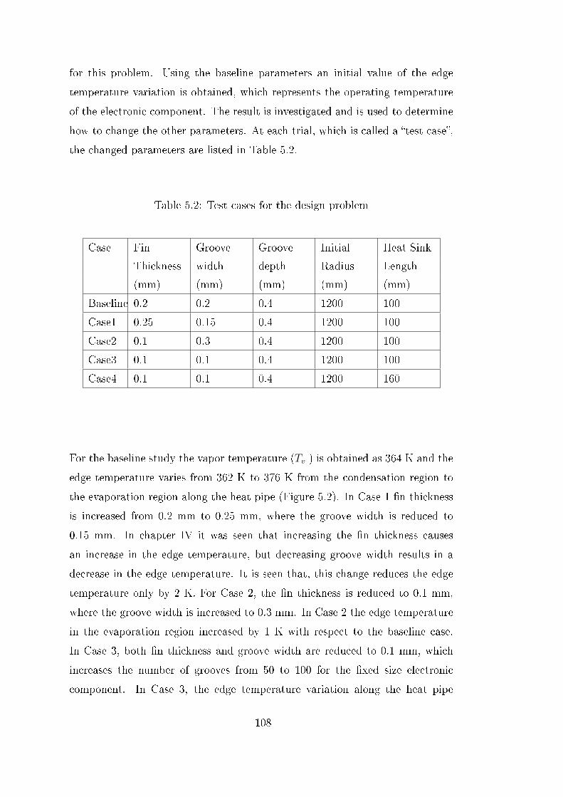
for this problem. Using the baseline parameters an initial value of the edge
temperature variation is obtained, which represents the operating temperature
of the electronic component. The result is investigated and is used to determine
how to change the other parameters. At each trial, which is called a test case,
the changed parameters are listed in Table 5.2.
Table 5.2: Test cases for the design problem
Case Fin Groove Groove Initial Heat Sink
Thickness width depth Radius Length
(mm) (mm) (mm) (mm) (mm)
Baseline 0.2 0.2 0.4 1200 100
Case1 0.25 0.15 0.4 1200 100
Case2 0.1 0.3 0.4 1200 100
Case3 0.1 0.1 0.4 1200 100
Case4 0.1 0.1 0.4 1200 160
For the baseline study the vapor temperature (Tv ) is obtained as 364 K and the
edge temperature varies from 362 K to 376 K from the condensation region to
the evaporation region along the heat pipe (Figure 5.2). In Case 1 n thickness
is increased from 0.2 mm to 0.25 mm, where the groove width is reduced to
0.15 mm. In chapter IV it was seen that increasing the n thickness causes
an increase in the edge temperature, but decreasing groove width results in a
decrease in the edge temperature. It is seen that, this change reduces the edge
temperature only by 2 K. For Case 2, the n thickness is reduced to 0.1 mm,
where the groove width is increased to 0.3 mm. In Case 2 the edge temperature
in the evaporation region increased by 1 K with respect to the baseline case.
In Case 3, both n thickness and groove width are reduced to 0.1 mm, which
increases the number of grooves from 50 to 100 for the xed size electronic
component. In Case 3, the edge temperature variation along the heat pipe
108

drops to 363368 K. However, the result is not sucient, because the dened
design temperature of 355 K cannot be obtained. All three cases do not provide
an acceptable change for the temperature. Moreover, in Chapter IV, it was
seen that changing the initial radius and the the groove depth did not aect the
edge temperature considerably. Therefore, the length of the heat sink region is
increased to 160 mm, where adiabatic region length of 60 mm in the baseline
case is also used for cooling. In section 4.2.9 it was shown that decreasing the
length of adiabatic region results in a decrease in the edge temperature. The
edge temperature range is reduced to 346353 K for Case 4, which is just below
the dened maximum allowable operating temperature and total uid mass to
be lled in the heat pipe is 2.9 grams.
The variation of the interface radius is given in Figure 5.1 and maximum edge
temperatures for each test case are summarized in Figure 5.3.
0.0E+00
2.0E-04
4.0E-04
6.0E-04
8.0E-04
1.0E-03
1.2E-03
1.4E-03
0 0.02 0.04 0.06 0.08 0.1 0.12 0.14 0.16 0.18 0.2
Axial position (m)
Inte
rface r
ad
ius (
m)
Baseline
Case 1
Case 2
Case 3
Case4
Figure 5.1: Liquid interface radius variation along heat pipe axis
109

340
345
350
355
360
365
370
375
380
0 0.02 0.04 0.06 0.08 0.1 0.12 0.14 0.16 0.18 0.2
Axial position (m)
Co
rner
tem
pera
ture
(K
)
Baseline
Case 1
Case 2
Case 3
Case 4
Op. Temp.
Figure 5.2: Edge temperature variation along heat pipe axis
350
355
360
365
370
375
380
Baseline Case 1 Case 2 Case 3 Case 4
Maxim
um
co
rner
tem
peart
ure
(K
)
Figure 5.3: Maximum edge temperature for test cases
110

CHAPTER 6
CONCLUSION
Heat pipes take advantage of phase change to remove heat generated from a
source. Therefore, they have large heat removal capacity compared to their
size, which makes them preferable especially for electronics cooling applications.
Studies performed on heat pipes with homogeneous wick structure used more
detailed analysis both with in-house developed or commercially available codes.
These studies involved two or three dimensional momentum analysis for liquid
and/or vapor ow as well as heat transfer analysis in heat pipe container. In
these studies evaporation/condensation mass ow rates were correlated by the
heat ux at the liquidvapor interface. However, studies on grooved heat pipes
used simplifying assumptions to model liquid and/or vapor ow. Some studies
included only axial heat in the analysis.
In the present study a at micro heat pipe with rectangular cross section is
investigated. Solution domain includes the heat pipe container material, solid
domain, and working uid, liquid domain. Previous studies showed that axial
conduction aects evaporation and condensation regions in the heat pipe, but
simplied approaches were used to model the heat transfer analysis. However,
in the present study solid and liquid domains are modeled by three dimensional
heat transfer equation. Phase change heat transfer from micro region is calcu-
lated using the relation obtained from kinetic theory. Moreover, phase change
heat transfer from macro region is included into the analysis calculated from the
heat balance at the liquidvapor interface. It is shown that macro evaporation
can account for up to 80% of the overall evaporation heat transfer. Conden-
111

sation from macro region is also calculated, however, it's eect on the overall
condensation heat transfer is found to be at most 15%. Energy equation in the
liquid domain includes both conduction and convection heat transfer, where the
eect of convection is negligible similar to the ndings of previous studies.
The results of the present study are validated using the results given in [6] in
terms of liquidvapor interface radius and heat pipe edge temperature variation
along the heat pipe axis. The dierence between two studies is found to be
acceptable, where the dierence is attributed to the three dimensional heat
transfer analysis and phase change modeling at the liquidvapor interface.
Due to the high thermal conductivity of the heat pipe container material, previ-
ous studies showed that a small fraction of the input heat load is transferred by
conduction through the container. However, according to the present study it is
found that %120 of the heat load is transferred by conduction inside the heat
pipe container and the working uid the magnitude of which is aected by the
length of heat source and heat sink regions. The percentage can be increased by
adding an adiabatic region at the outside boundary of the heat pipe between the
heat source and sink regions or decreasing the thermal conductivity of the heat
pipe material, which eectively reduces the contribution of the axial conduction.
In the current study the eects of physical dimensions of the heat pipe and
boundary conditions are also investigated. In the rst part of the study a denite
amount of heat load is applied and it is not forced to reach dry-out limit, the
variation of the liquidvapor interface and heat pipe container temperature,
which denes the operating range of the heat pipe is investigated. The results
can be summarized as,
• Increasing heat load increases the vapor temperature and consequently
higher heat pipe container temperature is obtained,
• Increasing ambient heat transfer coecient decreases heat pipe container
temperature,
• Decreasing heat pipe material thermal conductivity increases the ratio of
the heat transfer by phase change and increases the heat pipe container
112

temperature ,
• Increasing the initial value of the liquidvapor interface radius does not
aect the container temperature and the ratio of the heat transfer by phase
change, but the the interface radius change rate increases,
• Increasing groove depth decreases the ratio of the heat transfer by phase
change but does not change the container temperature,
• Increasing n thickness decreases the ratio of the heat transfer by phase
change, but increases the container temperature,
• Increasing groove width decreases the ratio of the heat transfer by phase
change, but increases the container temperature,
• Adding an adiabatic region or increasing it's length increase the ratio of
the heat transfer by phase change.
In the second part of the study, the eect of the physical dimension of the heat
pipe is investigated, where operation at the dry-out limit is forced by increasing
the input heat load. In this study, the change in the maximum heat transfer
capacity can be summarized as,
• For a xed total length of n thickness and groove width, increasing groove
width increases maximum heat transfer capacity until it reaches a upper
limit, where the capacity gets a constant value,
• For a constant n thickness, increasing groove width increases the heat
transfer capacity to a maximum, after which it starts to decrease,
• For a constant n thickness and groove width, increasing groove depth
increases heat capacity,
• Increasing heat pipe length decreases heat transfer capacity,
• Increasing the ratio of heat source and sink region lengths to the total
length decreases heat capacity.
113

Present study can be also used for dierent groove geometries (e.g trapezoidal)
and the eect of the geometry on the heat transfer capacity can be compared.
The thermophysical properties of the working uid is taken as constant values
in this study, the variation of those properties with temperature can be intro-
duced into the model, whose eect can be considerable where the vapor and the
edge temperature have high values. Moreover, vapor domain and vapor core
dimension can be included, which is not considered in the present model. The
eect of the vapor core dimension on the ooding limit can be analyzed. Con-
densation modeling of the present study uses simplied modeling of the liquid
lm thickness, which can be improved by detailed analysis and the eect on
the liquidvapor interface can be studied. The current condensation modeling,
which is also used in the previous studies, is not a mass conserving model, where
the condensate uid mass on the n top increases along the heat pipe axis from
the condensation region to the evaporation region. Moreover, the transition from
the condensation to the evaporation region on the n top is an abrupt change,
where the uid mass on the n top at the last condensation region position is
assumed to be evaporated completely at the rst evaporation region position
due to the phase change modeling. This condition can also aect the total uid
mass calculation, which considers both the liquid in the groove and on the n top
of the heat pipe geometry. By using more detailed condensation modeling the
analysis can be improved to analyze physical phenomena through phase change
region.
114

REFERENCES
[1] D. REAY P. KEW. Theory, Design and Application. Elsevier, 2006.
[2] T.NGUYEN K.MASHIKO Y.SAITO V.WUTTIJUMNONGM.MOCHIZUKI. A review of heat pipe application including newopportunities. Frontiers in Heat Pipes, 2-013001:115, 2011.
[3] B.R.BABIN G.P.PETERSON D.WU. Steady-state modeling and testingof a micro heat pipe. Journal of Heat Transfer, 112:595601, 1990.
[4] M.C.ZAGHDOUDI S.MAALEJ J.MANSOURI M.B.H.SASSI. Flat minia-ture heat pipes for electronics cooling: State of the art, experimental andtheoretical analysis. World Academy of Science, Engineering and Technol-
ogy, 75:880903, 2011.
[5] Y.WANG K.VAFAI. An experimental investigation of the thermal perfor-mance of an asymmetrical at plate heat pipe. International Journal of
Heat and Mass Transfer, 43:26572668, 2000.
[6] F.LEFÈVRE R.RULLIÈRE G.PANDRAUD M.LALLEMAND. Predictionof the temperature eld in at plate heat pipes with micro-grooves ex-perimental validation. International Journal of Heat and Mass Transfer,51:40834094, 2008.
[7] A.FAGHRI. Heat Pipe Science and Technology. Taylor and Francis, 1995.
[8] A.BEJAN A.KRAUS. Heat Transfer Handbook. John Wiley and Sons,2003.
[9] K.VAFAI W.WANG. Analysis of ow and heat transfer characteristics ofan asymmetrical at plate heat pipe. International Journal of Heat and
Mass Transfer, 35:20872099, 1992.
[10] N.ZHU K.VAFAI. Vapor and liquid ow in an asymmetrical at plate heatpipe: A threedimensional analytical and numerical investigation. Interna-tional Journal of Heat and Mass Transfer, 41(1):159174, 1998.
[11] Y.WANG K.VAFAI. Transient characterization of at plate heat pipesduring startup and shutdown operations. International Journal of Heat
and Mass Transfer, 43:26412655, 2000.
115

[12] B.XIAO A.FAGHRI. A three-dimensional thermal-uid analysis of at heatpipes. International Journal of Heat and Mass Transfer, 51:31133126,2008.
[13] M.AGHVAMI A.FAGHRI. Analysis of at heat pipes with various heat-ing and cooling congurations. Applied Thermal Engineering, 3:26452655,2011.
[14] J.H.PARK H.NOH J.LEE. A numerical study on the heat pipe withswitched heat source and sink for space application. ASME Proceedings
of 31st National Heat Transfer Conference, 7:109116, 1996.
[15] F.LEFÈVRE M.LALLEMAND. Coupled thermal and hydrodynamic mod-els of at micro heat pipes for the cooling of multiple electronic components.International Journal of Heat and Mass Transfer, 49:13751383, 2006.
[16] R.SONAN S.HARMAND J.PELLÈ D.LEGER M.FAKÈS. Transient ther-mal and hydrodynamic model of at heat pipe for the cooling of elec-tronics components. International Journal of Heat and Mass Transfer,51:60066017, 2008.
[17] N.THUCHAYAPONG A.NAKANO P.SAKULCHANGSATJATAIP.TERDTOON. Eect of capillary pressure on performance of aheat pipe: Numerical approach with fem. Applied Thermal Engineering,32:9399, 2012.
[18] M.ELNAGGAR M.Z.ABDULLAH M.A.MUJEEBU. Characterization ofworking uid in vertically mounted nned u-shape twin heat pipe for elec-tronic cooling. Energy Conversion and Management, 62:3139, 2012.
[19] V.BIANCO K.VAFAI O.MANCA M.SHAFAH. Thermal performance ofat-shaped heat pipes using nanouids. International Journal of Heat andMass Transfer, 53:14381445, 2010.
[20] G.P.PETERSON H.B.MA. Theoretical analysis of the maximum heattransport in triangular grooves: A study of idealized micro heat pipes.Journal of Heat Transfer, 118:731739, 1996.
[21] D.KHRUSTALEV A.FAGHRI. Thermal analysis of a micro heat pipe.Journal of Heat Transfer, 116:189198, 1994.
[22] M.R.KUMAR S.DASGUPTA. Modelling of evaporation from v-shaped mi-crogrooves. Chemical Engineer Community, 160:225248, 1997.
[23] B.SUMAN S.DE S.DASGUPTA. A model of the capillary limit of a microheat pipe and prediction of the dry-out length. International Journal of
Heat and Fluid Flow, 26:495505, 2005.
116
[24] B.SUMAN N.HODA. Eect of variations in thermophysical properties anddesign parameters on the performance of a v-shaped micro grooved heatpipe. International Journal of Heat and Mass Transfer, 48:20902101, 2005.
[25] B.SUMAN S.DE S.DASGUPTA. Transient modeling of micro-grooved heatpipe. International Journal of Heat and Mass Transfer, 48:16331646, 2005.
[26] S.ANAND S.DE S.DASGUPTA. Experimental and theoretical study of ax-ial dryout point for evaporation from v-shaped microgrooves. InternationalJournal of Heat and Mass Transfer, 45:15351543, 2002.
[27] S.K.THOMAS R.C.LYKINS K.L.YERKES. Fully developed laminar owin trapezoidal grooves with shear stress at the liquid-vapor interface. In-
ternational Journal of Heat and Mass Transfer, 44:33973412, 2001.
[28] S.LAUNAY V.SARTRE M.LALLEMAND. Hydrodynamic and thermalstudy of a water-lled micro-heat-pipe array. Journal of Thermophysics
and Heat Transfer, 18(3):358363, 2004.
[29] Y.M.HUNG K.TIO. Thermal analysis of optimally designed inclined microheat pipes with axial solid wall conduction. International Communications
in Heat and Mass Transfer, 39:11461153, 2012.
[30] F.L.CHANG Y.M.HUNG. The coupled eects of working uid and solidwall on thermal performance of micro heat pipes. International Communi-
cations in Heat and Mass Transfer, 73:7687, 2014.
[31] J.QU H.WU P.CHENG. Eects of functional surface on performance of amicro heat pipe. International Communications in Heat and Mass Transfer,35:523528, 2008.
[32] Y.CHEN C.ZHANG M.SHI J.WUA G.P.PETERSON. Study on ow andheat transfer characteristics of heat pipe with axial omega-shaped microgrooves. International Journal of Heat and Mass Transfer, 52:636643,2009.
[33] A.R. ANAND A.J. VEDAMURTHY S.R. CHIKKALA S. KUMAR D.KUMAR P. GUPTA. Analytical and experimental investigations on ax-ially grooved aluminum-ethane heat pipe. Heat Transfer Engineering,29(4):410416, 2008.
[34] S.J.KIM J.K.SEO K.H.DO. Analytical and experimental investigation onthe operational characteristics and the thermal optimization of a miniatureheat pipe with a grooved wick structure. International Journal of Heat andMass Transfer, 46:20512063, 2003.
[35] B.SUMAN. A steady state model and maximum heat transport capacityof an electrohydrodynamically augmented micro-grooved heat pipe. Inter-national Journal of Heat and Mass Transfer, 4:39573967, 2006.
117

[36] Y.M.HUNG Q.SENG. Eects of geometric design on thermal performanceof star-groove micro-heat pipes. International Journal of Heat and Mass
Transfer, 54:11981209, 2011.
[37] N.CHAURIS V.AYEL Y.BERTIN C.ROMESTANT D.EYSSERIC. Hy-draulic modelling of a at heat pipe with two dierent groove shapes anda small vapour section. Applied Thermal Engineering, 61:311 326, 2013.
[38] K.H.DO S.J.KIM S.V.GARIMELLA. A mathematical model for analyzingthe thermal characteristics of a at micro heat pipe with a grooved wick.International Journal of Heat and Mass Transfer, 51:46374650, 2008.
[39] C.GILLOT Y.AVENAS N.CEZAC G.POUPON C.SCHAEFFERE.FOURNIER. Silicon heat pipes used as thermal spreaders. , IEEE
Transactions on Components and Packaging Technologies, 26(2):332339,2003.
[40] L.LIN R.PONNAPPAN J.LELAND. High performance miniature heatpipe. International Journal of Heat and Mass Transfer, 45:31313142, 2002.
[41] R.RULLIÈRE F.LEFÈVRE M.LALLEMAND. Prediction of the maximumheat transfer capability of two-phase heat spreadersexperimental valida-tion. International Journal of Heat and Mass Transfer, 50:12551262, 2007.
[42] S.LIPS F.LEFÈVRE J.BONJOUR. Combined eects of the lling ratioand the vapour space thickness on the performance of a at plate heatpipe. International Journal of Heat and Mass Transfer, 53:694702, 2010.
[43] S.LIPS F.LEFÈVRE J.BONJOUR. Physical mechanisms involved ingrooved at heat pipes: Experimental and numerical analyses. Interna-
tional Journal of Thermal Sciences, 50:12431252, 2011.
[44] C.GILLOT A.LAR M.IVANOVA Y.AVENAS C.SCHAEFFERE.FOURNIER. Experimental study of a at silicon heat pipe withmicrocapillary grooves. Inter Society Conference on Thermal Phenomena,page 4750, 2004.
[45] Y.WANG G.P.PETERSON. Investigation of a novel at heat pipe. Journalof Heat Transfer, 127:165170, 2005.
[46] K.H.DO S.P.JANG. Eect of nanouids on the thermal performance of aat micro heat pipe with a rectangular grooved wick. International Journalof Heat and Mass Transfer, 53:21832192, 2010.
[47] P.C.STEPHAN C.A.BUSSE. Analysis of the heat transfer coecient ofgrooved heat pipe evaporator walls. International Journal of Heat and
Mass Transfer, 35(2):383391, 1992.
118

[48] S.DU Y.H.ZHAO. New boundary conditions for the evaporating thin-lmmodel in a rectangular micro channel. International Journal of Heat and
Mass Transfer, 54:36943701, 2011.
[49] R.BERTOSSI V.AYEL C.ROMESTANT Y.BERTIN Z.LATAOUI. Model-ing of transfer in the microregion in axially grooved heat pipes: Comparisonof uid performances. Heat Pipe Science and Technology, An International
Journal, 1(1):99112, 2010.
[50] A.J.JIAO H.B.MA J.K.CRITSER. Evaporation heat transfer characteris-tics of a grooved heat pipe with micro-trapezoidal grooves. International
Journal of Heat and Mass Transfer, 50:29052911, 2007.
[51] P.CHENG J.DONG S.M.THOMPSON H.B.MA. Heat transfer in bulkand thin-lm uid regions of rectangular microgroove. Journal of Ther-
mophysics and Heat Transfer, 26(1):108114, 2012.
[52] Y.ZHANG A.FAGHRI. Numerical simulation of condensation on a capil-lary grooved structure. Numerical Heat Transfer, Part A, page 227243,2001.
[53] R.H.NILSON S.W.TCHIKANDA S.K.GRIFFITHS M.J.MARTINEZ.Steady evaporating ow in rectangular microchannel. International Journalof Heat and Mass Transfer, 49:16031618, 2006.
119

120

APPENDIX A
DERIVATION OF ENERGY EQUATION IN THE
TRANSFORMED DOMAIN
u∂T
∂y+ w
∂T
∂z=
klρCpl
(∂2T
∂x2+∂2T
∂y2+∂2T
∂z2
)+
µ
ρlCplΦ (A.1)
The derivatives are written using chain rule.
∂T
∂y=
∂T
∂λ
∂λ
∂y+∂T
∂η
∂η
∂y+∂T
∂ξ
∂ξ
∂y(A.2)
∂2T
∂x2=
∂2T
∂λ2
(∂λ
∂x
)2
+∂2T
∂η2
(∂η
∂x
)2
+∂2T
∂ξ2
(∂ξ
∂x
)2
+
∂2T
∂λ∂η
(2∂λ
∂x
∂η
∂x
)+
∂2T
∂λ∂ξ
(2∂λ
∂x
∂ξ
∂x
)+
∂2T
∂η∂ξ
(2∂η
∂x
∂ξ
∂x
)+
∂T
∂λ
(∂2λ
∂x2
)+∂T
∂η
(∂2η
∂x2
)+∂T
∂ξ
(∂2ξ
∂x2
)(A.3)
∂2T
∂y2=
∂2T
∂λ2
(∂λ
∂y
)2
+∂2T
∂η2
(∂η
∂y
)2
+∂2T
∂ξ2
(∂ξ
∂y
)2
+
∂2T
∂λ∂η
(2∂λ
∂y
∂η
∂y
)+
∂2T
∂λ∂ξ
(2∂λ
∂y
∂ξ
∂y
)+
∂2T
∂η∂ξ
(2∂η
∂y
∂ξ
∂y
)+
∂T
∂λ
(∂2λ
∂y2
)+∂T
∂η
(∂2η
∂y2
)+∂T
∂ξ
(∂2ξ
∂y2
)(A.4)
121

∂2T
∂z2=
∂2T
∂λ2
(∂λ
∂z
)2
+∂2T
∂η2
(∂η
∂z
)2
+∂2T
∂ξ2
(∂ξ
∂z
)2
+
∂2T
∂λ∂η
(2∂λ
∂z
∂η
∂z
)+
∂2T
∂λ∂ξ
(2∂λ
∂y
∂ξ
∂z
)+
∂2T
∂η∂ξ
(2∂η
∂z
∂ξ
∂z
)+
∂T
∂λ
(∂2λ
∂z2
)+∂T
∂η
(∂2η
∂z2
)+∂T
∂ξ
(∂2ξ
∂z2
)(A.5)
The transformed coordinates are dened as follows
λ = x ; η = y ; ξ = z0 +z
4hi4h0 (A.6)
Therefore the following derivatives can be obtained directly.
∂λ
∂x= 1 ;
∂λ
∂y= 0 ;
∂λ
∂z= 0 ; (A.7)
∂η
∂x= 0 ;
∂η
∂y= 1 ;
∂η
∂z= 0 . (A.8)
Total derivative of each variable can be expressed in terms of and
dx =∂x
∂λdλ+
∂x
∂ηdη +
∂x
∂ξdξ ; (A.9)
dy =∂y
∂λdλ+
∂y
∂ηdη +
∂y
∂ξdξ ; (A.10)
dz =∂z
∂λdλ+
∂z
∂ηdη +
∂z
∂ξdξ . (A.11)
Equations A.11-13 are rearranged to give,
dλ =1
detJ[a1dx+ a2dy + a3dz] (A.12)
122

dη =1
detJ[b1dx+ b2dy + b3dz] (A.13)
dξ =1
detJ[c1dx+ c2dy + c3dz] (A.14)
where the coecients are,
a1 =∂y
∂η
∂z
∂ξ− ∂y
∂ξ
∂z
∂ηa2 =
∂x
∂ξ
∂z
∂η− ∂x
∂η
∂z
∂ξa3 =
∂x
∂η
∂y
∂ξ− ∂x
∂ξ
∂y
∂η
b1 =∂y
∂ξ
∂z
∂λ− ∂y
∂λ
∂z
∂ξb2 =
∂x
∂λ
∂z
∂ξ− ∂x
∂ξ
∂z
∂λb3 =
∂x
∂ξ
∂y
∂λ− ∂x
∂λ
∂y
∂ξ
c1 =∂y
∂λ
∂z
∂η− ∂y
∂η
∂z
∂λc2 =
∂x
∂η
∂z
∂λ− ∂x
∂λ
∂z
∂ηc3 =
∂x
∂λ
∂y
∂η− ∂x
∂η
∂y
∂λ
where J is the determinant of the Jacobian matrix and is dened as,
detJ = d1∂x
∂λ− d2
∂x
∂η+ d3
∂x
∂ξ(A.15)
where
d1 =∂y
∂η
∂z
∂ξ− ∂z
∂η
∂y
∂ξd2 =
∂y
∂λ
∂z
∂ξ− ∂z
∂λ
∂y
∂ξd3 =
∂y
∂λ
∂z
∂η− ∂z
∂λ
∂y
∂η
The Jacobian matrix is dened by,
∂λ
∂x
∂λ
∂y
∂λ
∂z
∂η
∂x
∂η
∂y
∂η
∂z
∂ξ
∂x
∂ξ
∂y
∂ξ
∂z
(A.16)
Using Equations A.9 and A.10 and A.18 following relations are derived.
123

∂x
∂λ= 1 ;
∂y
∂λ= 0 ;
∂z
∂λ= 0 ; (A.17)
∂x
∂η= 0 ;
∂y
∂η= 1 ;
∂z
∂η= 0. (A.18)
Coordinate derivatives becomes
∂λ
∂x= 1 ;
∂λ
∂y= 0 ;
∂λ
∂z= 0 ; (A.19)
∂η
∂x= 0 ;
∂η
∂y= 1 ;
∂η
∂z= 0 ; (A.20)
∂ξ
∂x= −∂z
∂λ/∂z
∂ξ;
∂ξ
∂y= −∂z
∂η/∂z
∂ξ;
∂ξ
∂z= 1/
∂z
∂ξ(A.21)
∂2λ
∂x2= 0 ;
∂2λ
∂y2= 0 ;
∂2λ
∂z2= 0 ; (A.22)
∂2η
∂x2= 0 ;
∂2η
∂y2= 0 ;
∂2η
∂z2= 0 . (A.23)
∂2ξ
∂x2= e1
(∂z
∂ξ
)−1+ e2
(∂z
∂ξ
)−2+ e3
(∂z
∂ξ
)−3∂2ξ
∂y2= f1
(∂z
∂ξ
)−1+ f2
(∂z
∂ξ
)−2+ f3
(∂z
∂ξ
)−3∂2ξ
∂z2= g1
(∂z
∂ξ
)−3(A.24)
where
124

e1 = −∂2z
∂λ2; e2 = 2
∂z
∂λ
∂2λ
∂ξ∂z; e3 = −∂
2z
∂ξ2
(∂z
∂λ
)2
;
f1 = −∂2z
∂η2; f2 = 2
∂z
∂η
∂2η
∂ξ∂z; f3 = −∂
2z
∂ξ2
(∂z
∂η
)2
;
g1 =∂2z
∂ξ2·
Final form of Equation A.1 becomes
u
(∂T
∂η+ h0
∂T
∂ξ
)+ w
(h1∂T
∂ξ
)=
klρCpl
(∂2T
∂λ2+∂2T
∂η2+ h2
∂2T
∂ξ2
)+
klρCpl
(h3
∂2T
∂λ∂ξ+ h4
∂2T
∂η∂ξ+ h5
∂T
∂ξ
)+
µ
ρlCplΦ (A.25)
where the coecients are dened as,
h0 =∂ξ
∂y
h1 =∂ξ
∂z
h2 =
(∂ξ
∂x
)2
+
(∂ξ
∂y
)2
+
(∂ξ
∂z
)2
h3 = 2∂ξ
∂x
h4 = 2∂ξ
∂y
h5 =∂2ξ
∂x2+∂2ξ
∂y2+∂2ξ
∂z2
125

126
APPENDIX B
ENERGY BALANCE EQUATIONS AT THE
INTERFACES
For the interface grid points between solid and liquid domain, nite dierence
form of the energy balance equations are given for the four subregions. The
indices i, j and k represent the grid node points in x, y and z−directions in the
solid domain and λ, η and ξ−directions in the transformed liquid domain. The
representative gures are given to show the heat ux denitions, where only
heat balance in x− z plane is shown.
Heat ow rates in solid domain are dened as,
q′′
xsAx = ksAx∂T
∂x(B.1)
q′′
ysAy = ksAy∂T
∂y(B.2)
q′′
zsAz = ksAz∂T
∂z(B.3)
Heat ow rates in liquid domain are dened in transformed coordinates. The
cross-sectional area Ax is in y−z plane, Ay in x−z plane, which are approximated
as trapezoidal areas and calculated for each grid point using the solution domain
grid points. Az is the projected area on x− y plane.
127
q′′
xlAx = klAx
(∂T
∂λ+∂T
∂ξ
∂ξ
∂x
)(B.4)
q′′
ylAy = klAy
(∂T
∂η+∂T
∂ξ
∂ξ
∂y
)(B.5)
q′′
zlAz = klAz
(∂T
∂ξ
∂ξ
∂z
)(B.6)
For the general case for a liquid control volume, the upper and lower surfaces
are curved and the surface normal has components in x and y−coordinates.The areas Antx and Anty represent projected areas of the upper curved surface
on y − z plane and x − z plane respectively, which are also approximated as
trapezoidal areas and calculated using grid points. Anbx and Anby are projected
areas of the lower curved surface.
q′′
ntxAntx = klAntx
(∂T
∂λ+∂T
∂ξ
∂ξ
∂x
)(B.7)
q′′
ntyAnty = klAnty
(∂T
∂η+∂T
∂ξ
∂ξ
∂y
)(B.8)
q′′
nbxAnbx = klAnbx
(∂T
∂λ+∂T
∂ξ
∂ξ
∂x
)(B.9)
q′′
nbyAnby = klAnby
(∂T
∂η+∂T
∂ξ
∂ξ
∂y
)(B.10)
B.1 Energy Balance for Region I
Region I is dened at the interface along the bottom of the groove. The heat
uxes on each surface is shown in Figure B.1
128

xl
zl
zs
Liquid
Solid
i,j,k
x
z
Figure B.1: Energy balance for Region I
For this region Qnbx and Qnby are not dened, since this part of the control
volume is solid. Finite dierence forms of Equations B.13 and B.48 become,
Qi− 12,j,k = ks
∆zs2
∆yTi−1,j,k − Ti,j,k
∆xl(B.11)
Qi+ 12,j,k = ks
∆zs2
∆yTi+1,j,k − Ti,j,k
∆xl(B.12)
Qi,j− 12,k = ks
∆zs2
∆xlTi,j−1,k − Ti,j,k
∆y(B.13)
129

Qi,j+ 12,k = ks
∆zs2
∆xlTi,j+1,k − Ti,j,k
∆y(B.14)
Qi,j,k− 12
= ks∆xl∆yTi,j,k−1 − Ti,j,k
∆zs(B.15)
For Region I the coordinate derivatives ∂ξ/∂x and ∂ξ/∂y are zero due to the solid
domain interface. As opposed to solid domain the areas Ax, Ay are changing
along the coordinate axes, therefore they are dened by indices i and j. Same
notation is used also for Antx and Anty . Finite dierence forms of the Equations
B.46 become,
Qi− 12,j,k = klAx
i− 12
∂T
∂λ= klAx
i− 12
Ti−1,j,k − Ti,j,k∆λ
(B.16)
Qi+ 12,j,k = klAx
i+12
∂T
∂λ= klAx
i+12
Ti+1,j,k − Ti,j,k∆λ
(B.17)
Qi,j− 12,k = klAy
j− 12
∂T
∂η= klAy
j− 12
Ti,j−1,k − Ti,j,k∆η
(B.18)
Qi,j+ 12,k = klAy
j+12
∂T
∂η= klAy
j+12
Ti,j+1,k − Ti,j,k∆η
(B.19)
Qi,j,k+ 12
= klAz∂T
∂ξ
∂ξ
∂z= klAz
Ti,j,k+1 − Ti,j,k∆ξ
(∂ξ
∂z
)i,j,k+ 1
2
(B.20)
Heat ow rates on the upper curved surface is dened by
Qntx = klAntx
[(∂T
∂λ
)i,j,k+ 1
2
+
(∂T
∂ξ
∂ξ
∂x
)i,j,k+ 1
2
](B.21)
Qnty = klAnty
[(∂T
∂η
)i,j,k+ 1
2
+
(∂T
∂ξ
∂ξ
∂y
)i,j,k+ 1
2
](B.22)
130

where (∂T
∂λ
)i,j,k+ 1
2
=1
2
[Ti+1,j,k − Ti−1,j,k
2∆λ+Ti+1,j,k+1 − Ti−1,j,k+1
2∆λ
](B.23)
(∂T
∂ξ
∂ξ
∂x
)i,j,k+ 1
2
=Ti,j,k+1 − Ti,j,k
∆ξ
1
2
[(∂ξ
∂x
)i,j,k
+
(∂ξ
∂x
)i,j,k+1
](B.24)
(∂T
∂η
)i,j,k+ 1
2
=1
2
[Ti,j+1,k − Ti,j−1,k
2∆η+Ti,j+1,k+1 − Ti,j−1,k+1
2∆η
](B.25)
(∂T
∂ξ
∂ξ
∂y
)i,j,k+ 1
2
=Ti,j,k+1 − Ti,j,k
∆ξ
1
2
[(∂ξ
∂y
)i,j,k
+
(∂ξ
∂y
)i,j,k+1
](B.26)
The convective terms are obtained from net enthalpy ow into the control volume
given in Figure B.2.
i,j,k
y
z
Figure B.2: Enthalpy ow to Region I
mihi − moho − mtyhty + mtzhtz = 0 (B.27)
Enthalpy is dened assuming constant Cpl as h = Cpl (T − Tref ) and mass ow
rates and temperature values are calculated as below.
131

mi =1
2(uj−1 + uj) ρlAy
j− 12
Ti =1
2(Ti,j,k + Ti,j−1,k)
mo =1
2(uj+1 + uj) ρlAy
j+12
To =1
2(Ti,j,k + Ti,j+1,k)
mty =ujρlAnty Tty =1
2(Ti,j,k + Ti,j,k+1)
mtz =− mi + mo + mty Ttz =1
2(Ti,j,k + Ti,j,k+1)
B.2 Energy Balance for Region II
Region II is located at the bottom groove corner as shown in Figure B.3. One
fourth of the control volume is in the liquid domain and the rest is in the solid
domain. The dierence for this region comes from the area denition with
respect to Region I.
132

Solid Solid
Solid Liquid
zs
zl
xs xl
i,j,k
x
z
Figure B.3: Heat balance for Region II
Qi− 12,j,k = ks
∆zs + ∆zl2
∆yTi−1,j,k − Ti,j,k
∆xl(B.28)
Qi+ 12,j,k = ks
∆zs2
∆yTi+1,j,k − Ti,j,k
∆xl(B.29)
Qi,j− 12,k = ks
(∆xs + ∆xl
2
∆zs2
+∆xs
2
∆zl2
)Ti,j−1,k − Ti,j,k
∆y(B.30)
Qi,j+ 12,k = ks
(∆xs + ∆xl
2
∆zs2
+∆xs
2
∆zl2
)Ti,j+1,k − Ti,j,k
∆y(B.31)
Qi,j,k− 12
= ks∆xs + ∆xl
2∆y
Ti,j,k−1 − Ti,j,k∆zl
(B.32)
133
Qi,j,k+ 12
= ks∆xs
2∆y
Ti,j,k+1 − Ti,j,k∆zs
(B.33)
For Region II the coordinate derivatives ∂ξ/∂x and ∂ξ/∂y are zero and ∂ξ/∂z =
1 due to the solid domain interface. Finite dierence forms of the Equations
B.47 become,
Qi+ 12,j,k = klAx
i+12
∂T
∂λ= klAx
i+12
Ti+1,j,k − Ti,j,k∆λ
(B.34)
Qi,j− 12,k = klAy
j− 12
∂T
∂η= klAy
j− 12
Ti,j−1,k − Ti,j,k∆η
(B.35)
Qi,j+ 12,k = klAy
j+12
∂T
∂η= klAy
j+12
Ti,j+1,k − Ti,j,k∆η
(B.36)
Qi,j,k+ 12
= klAz∂T
∂ξ= klAz
Ti,j,k+1 − Ti,j,k∆ξ
(B.37)
Only the xcomponent of the Qnt is dened, since the surface normal at the
grid point i, j, k + 12is located on the solid line, where there is no variation in
y−direction. Heat ow rates on the upper curved surface is dened by
Qntx = klAntx
[(∂T
∂λ
)i,j,k+ 1
2
+
(∂T
∂ξ
∂ξ
∂x
)i,j,k+ 1
2
](B.38)
where
(∂T
∂λ
)i,j,k+ 1
2
=1
2
[Ti+1,j,k − Ti,j,k
∆λ+Ti+1,j,k+1 − Ti,j,k+1
∆λ
](B.39)
(∂T
∂ξ
∂ξ
∂x
)i,j,k+ 1
2
=Ti,j,k+1 − Ti,j,k
∆ξ
1
2
[(∂ξ
∂x
)i,j,k
+
(∂ξ
∂x
)i,j,k+1
](B.40)
The convective terms are obtained from net enthalpy ow into the control volume
given in Figure B.4. same as for Region I.
134
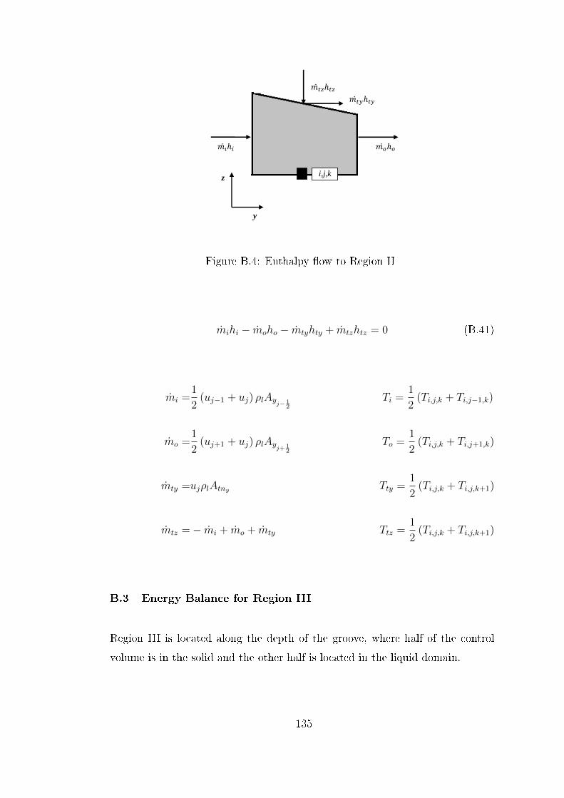
i,j,k
y
z
Figure B.4: Enthalpy ow to Region II
mihi − moho − mtyhty + mtzhtz = 0 (B.41)
mi =1
2(uj−1 + uj) ρlAy
j− 12
Ti =1
2(Ti,j,k + Ti,j−1,k)
mo =1
2(uj+1 + uj) ρlAy
j+12
To =1
2(Ti,j,k + Ti,j+1,k)
mty =ujρlAtny Tty =1
2(Ti,j,k + Ti,j,k+1)
mtz =− mi + mo + mty Ttz =1
2(Ti,j,k + Ti,j,k+1)
B.3 Energy Balance for Region III
Region III is located along the depth of the groove, where half of the control
volume is in the solid and the other half is located in the liquid domain.
135
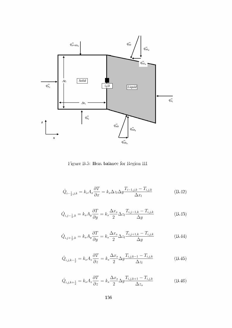
xs
zl Solid
Liquid
i,j,k
x
z
Figure B.5: Heat balance for Region III
Qi− 12,j,k = ksAx
∂T
∂x= ks∆zl∆y
Ti−1,j,k − Ti,j,k∆xl
(B.42)
Qi,j− 12,k = ksAy
∂T
∂y= ks
∆xs2
∆zlTi,j−1,k − Ti,j,k
∆y(B.43)
Qi,j+ 12,k = ksAy
∂T
∂y= ks
∆xs2
∆zlTi,j+1,k − Ti,j,k
∆y(B.44)
Qi,j,k− 12
= ksAz∂T
∂z= ks
∆xs2
∆yTi,j,k−1 − Ti,j,k
∆zl(B.45)
Qi,j,k+ 12
= ksAz∂T
∂z= ks
∆xs2
∆yTi,j,k+1 − Ti,j,k
∆zs(B.46)
136

Similar to Region II, in Region III the coordinate derivative ∂ξ/∂y is zero and
∂ξ/∂z = 1 due to the solid domain interface.
Qi+ 12,j,k = klAx
i+12
[(∂T
∂λ
)i+ 1
2,j,k
+
(∂T
∂ξ
∂ξ
∂x
)i+ 1
2,j,k
](B.47)
where
(∂T
∂λ
)i+ 1
2,j,k
=Ti+1,j,k − Ti,j,k
∆λ(B.48)
(∂T
∂ξ
∂ξ
∂x
)i+ 1
2,j,k
=1
2
[Ti,j,k+1 − Ti,j,k−1
2∆ξ+Ti+1,j,k+1 − Ti+1,j,k−1
2∆ξ
]
+1
2
[(∂ξ
∂x
)i,j,k
+
(∂ξ
∂x
)i+1,j,k
](B.49)
Qi,j− 12,k = klAy
j− 12
∂T
∂η= klAy
j− 12
Ti,j−1,k − Ti,j,k∆η
(B.50)
Qi,j+ 12,k = klAy
j+12
∂T
∂η= klAy
j+12
Ti,j+1,k − Ti,j,k∆η
(B.51)
Qi,j,k− 12
= klAz∂T
∂ξ= klAz
Ti,j,k−1 − Ti,j,k∆ξ
(B.52)
Qi,j,k+ 12
= klAz∂T
∂ξ= klAz
Ti,j,k+1 − Ti,j,k∆ξ
(B.53)
For Region III both Qnt and Qnb are considered.
Qntx = klAntx
[(∂T
∂λ
)i,j,k+ 1
2
+
(∂T
∂ξ
∂ξ
∂x
)i,j,k+ 1
2
](B.54)
Qnbx = klAnbx
[(∂T
∂λ
)i,j,k− 1
2
+
(∂T
∂ξ
∂ξ
∂x
)i,j,k− 1
2
](B.55)
137

where
(∂T
∂λ
)i,j,k+ 1
2
=1
2
[Ti+1,j,k − Ti,j,k
∆λ+Ti+1,j,k+1 − Ti,j,k+1
∆λ
](B.56)
(∂T
∂ξ
∂ξ
∂x
)i,j,k+ 1
2
=Ti,j,k+1 − Ti,j,k
∆ξ
1
2
[(∂ξ
∂x
)i,j,k
+
(∂ξ
∂x
)i,j,k+1
](B.57)
(∂T
∂λ
)i,j,k− 1
2
=1
2
[Ti,j,k − Ti+1,j,k
∆λ+Ti,j,k−1 − Ti+1,j,k−1
∆λ
](B.58)
(∂T
∂ξ
∂ξ
∂x
)i,j,k− 1
2
=Ti,j,k−1 − Ti,j,k
∆ξ
1
2
[(∂ξ
∂x
)i,j,k
+
(∂ξ
∂x
)i,j,k−1
](B.59)
The convective terms are obtained from net enthalpy ow into the control volume
given in Figure B.6.
i,j,k
y
z
Figure B.6: Enthalpy ow to Region III
mihi − moho − mtyhty + mtzhtz + mbyhby − mbzhbz = 0 (B.60)
138

mi =1
2(uj−1 + uj) ρlAy
j− 12
Ti =1
2(Ti,j,k + Ti,j−1,k)
mo =1
2(uj+1 + uj) ρlAy
j+12
To =1
2(Ti,j,k + Ti,j+1,k)
mty =ujρlAtny Tty =1
2(Ti,j,k + Ti,j,k+1)
mtz =− mi + mo + mty − mby + mbz Ttz =1
2(Ti,j,k + Ti,j,k+1)
mby =ujρlAbny Tby =1
2(Ti,j,k + Ti,j,k−1)
mbz =(−mtz)k− 12
Tbz =1
2(Ti,j,k + Ti,j,k−1)
B.4 Energy Balance for Region IV
Region IV is at n top corner, where upper surface is liquidvapor interface and
includes phase change as given in Figure B.7.
139

xs
zl Solid
Liquid
i,j,k
x
z
for evaporation for condensation
Figure B.7: Heat balance for Region IV
Heat ow rates in solid domain are dened as,
Qi− 12,j,k = ks
∆zl2
∆yTi−1,j,k − Ti,j,k
∆xs(B.61)
Qi,j− 12,k = ks
∆xs2
∆zl2
Ti,j−1,k − Ti,j,k∆y
(B.62)
Qi,j+ 12,k = ks
∆xs2
∆zl2
Ti,j+1,k − Ti,j,k∆y
(B.63)
Qi,j,k− 12
= ks∆xs
2∆y
Ti,j,k−1 − Ti,j,k∆zl
(B.64)
For condensation region, phase change is dened by a convection boundary con-
dition on the upper surface in the solid domain, whereas for evaporation region,
140

this surface is assumed to be insulated, where Qpc is taken as zero.
Qi,j,k = Qpc = hpc∆xs
2∆y (Tv − Ti,j,k) (B.65)
For Region IV the coordinate derivatives ∂ξ/∂y is zero and ∂ξ/∂z = 1 due to the
solid domain interface. Finite dierence forms of the Equations B.48 become,
Qi+ 12,j,k = klAx
i+12
[(∂T
∂λ
)i+ 1
2,j,k
+
(∂T
∂ξ
∂ξ
∂x
)i+ 1
2,j,k
](B.66)
where
(∂T
∂λ
)i+ 1
2,j,k
=Ti+1,j,k − Ti,j,k
∆λ(B.67)
(∂T
∂ξ
∂ξ
∂x
)i+ 1
2,j,k
=1
2
[Ti,j,k − Ti,j,k−1
∆ξ+Ti+1,j,k − Ti+1,j,k−1
∆ξ
]
+1
2
[(∂ξ
∂x
)i,j,k
+
(∂ξ
∂x
)i+1,j,k
](B.68)
Qi,j− 12,k = klAy
j− 12
∂T
∂η= klAy
j− 12
Ti,j−1,k − Ti,j,k∆η
(B.69)
Qi,j+ 12,k = klAy
j+12
∂T
∂η= klAy
j+12
Ti,j+1,k − Ti,j,k∆η
(B.70)
Qi,j,k− 12
= klAz∂T
∂ξ= klAz
Ti,j,k−1 − Ti,j,k∆ξ
(B.71)
In region IV for evaporation region it is assumed that Qnt is equal to the phase
change heat transfer and approximated with convection boundary condition.
Qnt = Qpc = hpc∆xl
2∆y (Ti,j,k − Tv) (B.72)
141

At the lower surface of the liquid domain
Qnbx = klAnbx
[(∂T
∂λ
)i,j,k− 1
2
+
(∂T
∂ξ
∂ξ
∂x
)i,j,k− 1
2
](B.73)
where
(∂T
∂λ
)i,j,k− 1
2
=1
2
[Ti,j,k − Ti+1,j,k
∆λ+Ti,j,k−1 − Ti+1,j,k−1
∆λ
](B.74)
(∂T
∂ξ
∂ξ
∂x
)i,j,k− 1
2
=Ti,j,k−1 − Ti,j,k
∆ξ
1
2
[(∂ξ
∂x
)i,j,k
+
(∂ξ
∂x
)i,j,k−1
](B.75)
The convective terms are obtained from net enthalpy ow into the control volume
given in Figure B.8.
i,j,k
y
z
Figure B.8: Enthalpy ow to Region IV
mihi − moho + mbyhby − mbzhbz + mpc (hlv + Tv) = 0 (B.76)
142

mpc represent phase change mass ow rate for both condensation and evapora-
tion and calculated by a mass balance dened as below.
mi =1
2(uj−1 + uj) ρlAy
j− 12
Ti =1
2(Ti,j,k + Ti,j−1,k)
mo =1
2(uj+1 + uj) ρlAy
j+12
To =1
2(Ti,j,k + Ti,j+1,k)
mby =ujρlAbny Tby =1
2(Ti,j,k + Ti,j,k−1)
mbz =(−mtz)k− 12
Tbz =1
2(Ti,j,k + Ti,j,k−1)
mpc =− mi + mo − mby + mbz
Since mpchlv is considered in overall energy balance, it is not included again in
convective terms.
B.5 Energy Balance for Region V
Region V is located fully in the liquid domain, where the heat uxes on each
face are shown in Figure B.9.
143
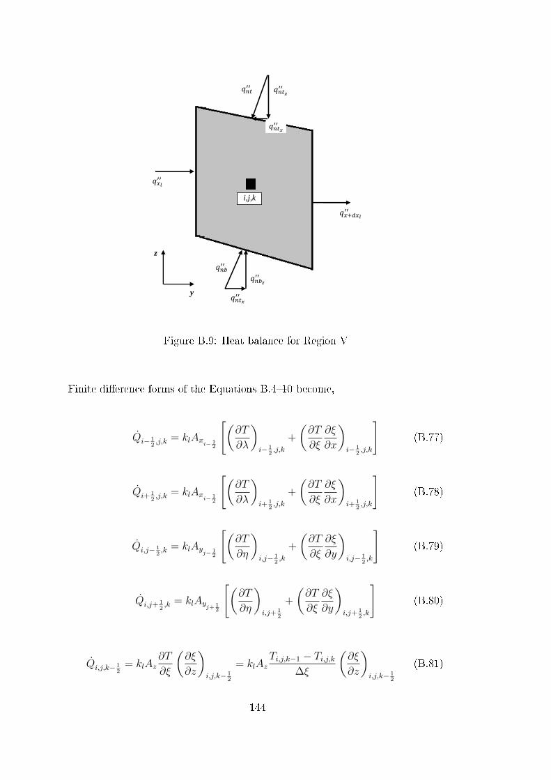
i,j,k
y
z
Figure B.9: Heat balance for Region V
Finite dierence forms of the Equations B.410 become,
Qi− 12,j,k = klAx
i− 12
[(∂T
∂λ
)i− 1
2,j,k
+
(∂T
∂ξ
∂ξ
∂x
)i− 1
2,j,k
](B.77)
Qi+ 12,j,k = klAx
i− 12
[(∂T
∂λ
)i+ 1
2,j,k
+
(∂T
∂ξ
∂ξ
∂x
)i+ 1
2,j,k
](B.78)
Qi,j− 12,k = klAy
j− 12
[(∂T
∂η
)i,j− 1
2,k
+
(∂T
∂ξ
∂ξ
∂y
)i,j− 1
2,k
](B.79)
Qi,j+ 12,k = klAy
j+12
[(∂T
∂η
)i,j+ 1
2
+
(∂T
∂ξ
∂ξ
∂y
)i,j+ 1
2,k
](B.80)
Qi,j,k− 12
= klAz∂T
∂ξ
(∂ξ
∂z
)i,j,k− 1
2
= klAzTi,j,k−1 − Ti,j,k
∆ξ
(∂ξ
∂z
)i,j,k− 1
2
(B.81)
144

Qi,j,k+ 12
= klAz∂T
∂ξ
(∂ξ
∂z
)i,j,k+ 1
2
= klAzTi,j,k+1 − Ti,j,k
∆ξ
(∂ξ
∂z
)i,j,k+ 1
2
(B.82)
where
(∂T
∂λ
)i− 1
2,j,k
=Ti−1,j,k − Ti,j,k
∆λ(B.83)
(∂T
∂λ
)i+ 1
2,j,k
=Ti+1,j,k − Ti,j,k
∆λ(B.84)
(∂T
∂η
)i,j− 1
2,k
=Ti,j−1,k − Ti,j,k
∆η(B.85)
(∂T
∂η
)i,j+ 1
2,k
=Ti,j+1,k − Ti,j,k
∆η(B.86)
(∂T
∂ξ
∂ξ
∂x
)i− 1
2,j,k
=1
2
[Ti,j,k−1 − Ti,j,k+1
2∆ξ+Ti−1,j,k−1 − Ti−1,j,k+1
2∆ξ
]
+1
2
[(∂ξ
∂x
)i,j,k
+
(∂ξ
∂x
)i−1,j,k
](B.87)
(∂T
∂ξ
∂ξ
∂x
)i+ 1
2,j,k
=1
2
[Ti,j,k+1 − Ti,j,k−1
2∆ξ+Ti+1,j,k+1 − Ti+1,j,k−1
2∆ξ
]
+1
2
[(∂ξ
∂x
)i,j,k
+
(∂ξ
∂x
)i+1,j,k
](B.88)
(∂T
∂ξ
∂ξ
∂y
)i,j− 1
2,k
=1
2
[Ti,j,k−1 − Ti,j,k+1
2∆ξ+Ti,j−1,k−1 − Ti,j−1,k+1
2∆ξ
]
+1
2
[(∂ξ
∂y
)i,j,k
+
(∂ξ
∂y
)i,j−1,k
](B.89)
145

(∂T
∂ξ
∂ξ
∂y
)i,j+ 1
2,k
=1
2
[Ti,j,k+1 − Ti,j,k−1
2∆ξ+Ti,j+1,k+1 − Ti,j+1,k−1
2∆ξ
]
+1
2
[(∂ξ
∂y
)i,j,k
+
(∂ξ
∂y
)i,j+1,k
](B.90)
At the lower surface of the liquid domain
Qnbx = klAnbx
[(∂T
∂λ
)i,j,k− 1
2
+
(∂T
∂ξ
∂ξ
∂x
)i,j,k− 1
2
](B.91)
Qnby = klAnby
[(∂T
∂η
)i,j,k− 1
2
+
(∂T
∂ξ
∂ξ
∂y
)i,j,k− 1
2
](B.92)
where
(∂T
∂λ
)i,j,k− 1
2
=1
2
[Ti−1,j,k − Ti+1,j,k
2∆λ+Ti−1,j,k−1 − Ti+1,j,k−1
2∆λ
](B.93)
(∂T
∂ξ
∂ξ
∂x
)i,j,k− 1
2
=Ti,j,k−1 − Ti,j,k
∆ξ
1
2
[(∂ξ
∂x
)i,j,k
+
(∂ξ
∂x
)i,j,k−1
](B.94)
(∂T
∂η
)i,j,k− 1
2
=1
2
[Ti,j−1,k − Ti,j+1,k
2∆η+Ti,j−1,k−1 − Ti,j+1,k−1
2∆η
](B.95)
(∂T
∂ξ
∂ξ
∂y
)i,j,k− 1
2
=Ti,j,k−1 − Ti,j,k
∆ξ
1
2
[(∂ξ
∂y
)i,j,k
+
(∂ξ
∂y
)i,j,k−1
](B.96)
At the upper surface of the liquid domain
Qntx = klAntx
[(∂T
∂λ
)i,j,k+ 1
2
+
(∂T
∂ξ
∂ξ
∂x
)i,j,k+ 1
2
](B.97)
Qnty = klAnty
[(∂T
∂η
)i,j,k+ 1
2
+
(∂T
∂ξ
∂ξ
∂y
)i,j,k+ 1
2
](B.98)
146

where
(∂T
∂λ
)i,j,k+ 1
2
=1
2
[Ti+1,j,k − Ti−1,j,k
2∆λ+Ti+1,j,k+1 − Ti−1,j,k+1
2∆λ
](B.99)
(∂T
∂ξ
∂ξ
∂x
)i,j,k+ 1
2
=Ti,j,k+1 − Ti,j,k
∆ξ
1
2
[(∂ξ
∂x
)i,j,k
+
(∂ξ
∂x
)i,j,k+1
](B.100)
(∂T
∂η
)i,j,k+ 1
2
=1
2
[Ti,j+1,k − Ti,j−1,k
2∆η+Ti,j+1,k+1 − Ti,j−1,k+1
2∆η
](B.101)
(∂T
∂ξ
∂ξ
∂y
)i,j,k+ 1
2
=Ti,j,k+1 − Ti,j,k
∆ξ
1
2
[(∂ξ
∂y
)i,j,k
+
(∂ξ
∂y
)i,j,k+1
](B.102)
The convective terms are obtained from net enthalpy ow into the control volume
given in Figure B.10.
i,j,k
y
z
Figure B.10: Enthalpy ow to Region V
mihi − moho − mtyhty + mtzhtz + mbyhby − mbzhbz = 0 (B.103)
147
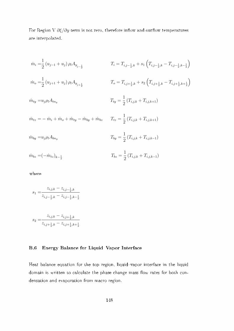
For Region V ∂ξ/∂y term is not zero, therefore inow and outow temperatures
are interpolated.
mi =1
2(uj−1 + uj) ρlAy
j− 12
Ti = Ti,j− 12,k + s1
(Ti,j− 1
2,k − Ti,j− 1
2,k− 1
2
)
mo =1
2(uj+1 + uj) ρlAy
j+12
To = Ti,j+ 12,k + s2
(Ti,j+ 1
2,k − Ti,j+ 1
2,k+ 1
2
)
mty =ujρlAtny Tty =1
2(Ti,j,k + Ti,j,k+1)
mtz =− mi + mo + mty − mby + mbz Ttz =1
2(Ti,j,k + Ti,j,k+1)
mby =ujρlAbny Tby =1
2(Ti,j,k + Ti,j,k−1)
mbz =(−mtz)k− 12
Tbz =1
2(Ti,j,k + Ti,j,k−1)
where
s1 =zi,j,k − zi,j− 1
2,k
zi,j− 12,k − zi,j− 1
2,k− 1
2
s2 =zi,j,k − zi,j+ 1
2,k
zi,j+ 12,k − zi,j+ 1
2,k+ 1
2
B.6 Energy Balance for LiquidVapor Interface
Heat balance equation for the top region, liquidvapor interface in the liquid
domain is written to calculate the phase change mass ow rates for both con-
densation and evaporation from macro region.
148

i,j,k
x
z
Figure B.11: Heat balance at the liquidvapor interface
Qi− 12,j,k = klAx
i− 12
[(∂T
∂λ
)i− 1
2,j,k
+
(∂T
∂ξ
∂ξ
∂x
)i− 1
2,j,k
](B.104)
Qi+ 12,j,k = klAx
i− 12
[(∂T
∂λ
)i+ 1
2,j,k
+
(∂T
∂ξ
∂ξ
∂x
)i+ 1
2,j,k
](B.105)
Qi,j− 12,k = klAy
j− 12
[(∂T
∂η
)i,j− 1
2,k
+
(∂T
∂ξ
∂ξ
∂y
)i,j− 1
2,k
](B.106)
Qi,j+ 12,k = klAy
j+12
[(∂T
∂η
)i,j+ 1
2
+
(∂T
∂ξ
∂ξ
∂y
)i,j+ 1
2,k
](B.107)
Qi,j,k− 12
= klAz∂T
∂ξ
(∂ξ
∂z
)i,j,k− 1
2
= klAzTi,j,k−1 − Ti,j,k
∆ξ
(∂ξ
∂z
)i,j,k− 1
2
(B.108)
where
149

(∂T
∂λ
)i− 1
2,j,k
=Ti−1,j,k − Ti,j,k
∆λ(B.109)
(∂T
∂λ
)i+ 1
2,j,k
=Ti+1,j,k − Ti,j,k
∆λ(B.110)
(∂T
∂η
)i,j− 1
2,k
=Ti,j−1,k − Ti,j,k
∆η(B.111)
(∂T
∂η
)i,j+ 1
2,k
=Ti,j+1,k − Ti,j,k
∆η(B.112)
(∂T
∂ξ
∂ξ
∂x
)i− 1
2,j,k
=1
2
[Ti,j,k−1 − Ti,j,k+1
2∆ξ+Ti−1,j,k−1 − Ti−1,j,k+1
2∆ξ
]
+1
2
[(∂ξ
∂x
)i,j,k
+
(∂ξ
∂x
)i−1,j,k
](B.113)
(∂T
∂ξ
∂ξ
∂x
)i+ 1
2,j,k
=1
2
[Ti,j,k+1 − Ti,j,k−1
2∆ξ+Ti+1,j,k+1 − Ti+1,j,k−1
2∆ξ
]
+1
2
[(∂ξ
∂x
)i,j,k
+
(∂ξ
∂x
)i+1,j,k
](B.114)
(∂T
∂ξ
∂ξ
∂y
)i,j− 1
2,k
=1
2
[Ti,j,k−1 − Ti,j,k+1
2∆ξ+Ti,j−1,k−1 − Ti,j−1,k+1
2∆ξ
]
+1
2
[(∂ξ
∂y
)i,j,k
+
(∂ξ
∂y
)i,j−1,k
](B.115)
(∂T
∂ξ
∂ξ
∂y
)i,j+ 1
2,k
=1
2
[Ti,j,k+1 − Ti,j,k−1
2∆ξ+Ti,j+1,k+1 − Ti,j+1,k−1
2∆ξ
]
+1
2
[(∂ξ
∂y
)i,j,k
+
(∂ξ
∂y
)i,j+1,k
](B.116)
150

At the lower surface of the liquid domain
Qnbx = klAnbx
[(∂T
∂λ
)i,j,k− 1
2
+
(∂T
∂ξ
∂ξ
∂x
)i,j,k− 1
2
](B.117)
Qnby = klAnby
[(∂T
∂η
)i,j,k− 1
2
+
(∂T
∂ξ
∂ξ
∂y
)i,j,k− 1
2
](B.118)
where
(∂T
∂λ
)i,j,k− 1
2
=1
2
[Ti−1,j,k − Ti+1,j,k
2∆λ+Ti−1,j,k−1 − Ti+1,j,k−1
2∆λ
](B.119)
(∂T
∂ξ
∂ξ
∂x
)i,j,k− 1
2
=Ti,j,k−1 − Ti,j,k
∆ξ
1
2
[(∂ξ
∂x
)i,j,k
+
(∂ξ
∂x
)i,j,k−1
](B.120)
(∂T
∂η
)i,j,k− 1
2
=1
2
[Ti,j−1,k − Ti,j+1,k
2∆η+Ti,j−1,k−1 − Ti,j+1,k−1
2∆η
](B.121)
(∂T
∂ξ
∂ξ
∂y
)i,j,k− 1
2
=Ti,j,k−1 − Ti,j,k
∆ξ
1
2
[(∂ξ
∂y
)i,j,k
+
(∂ξ
∂y
)i,j,k−1
](B.122)
The convective terms are obtained from net enthalpy ow into the control volume
given in Figure B.12.
151
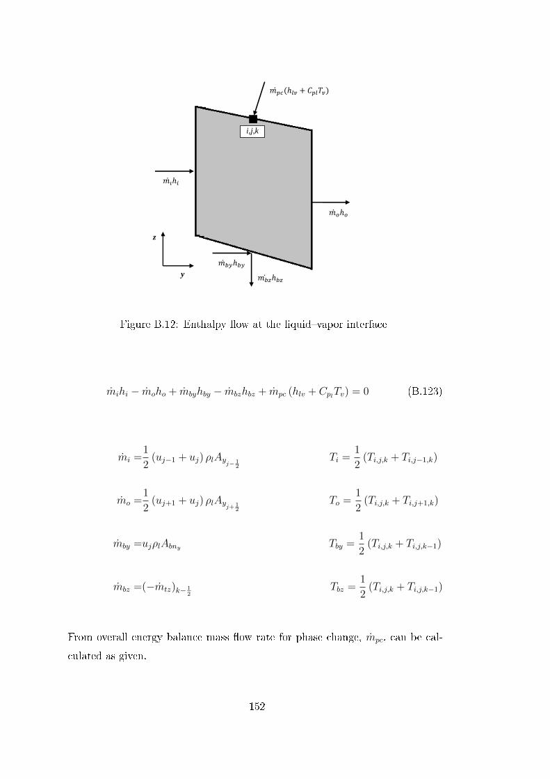
i,j,k
y
z
Figure B.12: Enthalpy ow at the liquidvapor interface
mihi − moho + mbyhby − mbzhbz + mpc (hlv + CplTv) = 0 (B.123)
mi =1
2(uj−1 + uj) ρlAy
j− 12
Ti =1
2(Ti,j,k + Ti,j−1,k)
mo =1
2(uj+1 + uj) ρlAy
j+12
To =1
2(Ti,j,k + Ti,j+1,k)
mby =ujρlAbny Tby =1
2(Ti,j,k + Ti,j,k−1)
mbz =(−mtz)k− 12
Tbz =1
2(Ti,j,k + Ti,j,k−1)
From overall energy balance mass ow rate for phase change, mpc, can be cal-
culated as given.
152

Qnet + miCpl (Ti − Tv)− moCpl (To − Tv) +
mbyCpl (Tby − Tv)− mbz (Tbz − Tv) + mpchlv = 0 (B.124)
153

154

CURRICULUM VITAE
PERSONAL INFORMATION
Surname, Name: ODABAI, Gülnihal
Nationality: Turkish (TC)
Date and Place of Birth: 1972, Ankara
Marital Status: Single
Phone: (533)2592750
Fax:
EDUCATION
Degree Institution Year of Graduation
M.S. METU 1997
B.S. METU 1995
High School Ankara Anatolian High School 1990
PROFESSIONAL EXPERIENCE
Year Place Enrollment
19972006 ROKETSAN Engineer
20062007 TUBITAK Space Technologies Research Institute Researcher
20072013 STM Defence Technologies and Engineering Certication Engineer
155

PUBLICATIONS
International Publications
DURSUNKAYA Z. ODABAI G. Numerical solution of solidication in a square
prism using an algebraic grid generation technique Heat and Mass Transfer, 40,
pp 9197, 2003
156


