Modeling of Natural Remediation: Contaminant Fate … of Natural Remediation: Contaminant Fate and...

September 1999 Page 1 of 57 MNR Chapter V5 0.doc

Modeling of Natural Remediation: Contaminant Fate and Transport Brent Peyton Assistant Professor, Chemical Engineering Department Center for Multiphase Environmental Research Washington State University Dana Hall 118, Spokane St. Pullman, WA 99164-2710 USA PH (509) 335-4002 FAX (509) 335-4806 E-mail: [email protected] John Connolly Quantitative Environmental Analysis, LLC 305 West Grand Avenue Montvale, NJ 07645 USA PH (201) 930-9890 FAX (201) 930-9805 E-mail: [email protected] Prabhakar Clement


Predictive models can play an important role in verifying the occurrence and significance of

natural remediation and can significantly improve the design of monitoring and assessment

procedures. Predictions resulting from the models can be used to address important questions

that invariably arise during the assessment of remediation by intrinsic processes. Such questions

may include the following: “Will environmentally important receptors be impacted by the

contaminant?; What are the expected average and maximum concentration levels and what is the

associated risk?; How long will it take for the contaminant plume to degrade below regulated

limits?” To answer these questions, one must adequately describe the key natural remediation

processes that are active at the site. To accomplish such description, robust mathematical

models capable of predicting the transport and reaction of contaminants are required.

Typically, models used to evaluate natural remediation modeling involves two distinct modeling

steps: 1) modeling the general environmental system (e.g., sediment, surface water, and/or

groundwater) and 2) modeling the transport and reaction of specific contaminants. Interactions

between contaminants and environmental materials often control the rates of natural remediation.

Partitioning of fuel hydrocarbons to soil organic matter can limit the rate of hydrocarbon

transport and also the rate of bacterial degradation. The interactions might be sufficiently

important that they may modify the properties of the system itself. One case where interactions

of this type can be important is when rapid microbial growth during an in situ bioremediation

effort might significantly reduce the permeability and porosity of the porous media (Taylor and

Jaffe, 1990; Clement et al., 1996b). However, for most natural remediation modeling

applications, the flow and reactive transport may be considered as uncoupled processes.


For complex environmental systems such as those typically encountered at contaminated sites,

computer models will never give answers that accurately reflect all aspects of the complex

chemical and microbial interactions that may be occurring. For natural remediation, rather than

giving “answers”, models should be used to predict future trends and to provide insight into the

relative importance of various processes that are occurring at the site. In this way, a natural

remediation model can be used as a project mentor, rather than as a project director. Complex

models such as these are subject to many conditions that may severely limit the accuracy or

applicability of a particular model to a particular site. These limitations may or may not be

known at the time the natural remediation assessment begins. During an initial site

characterization, for example, based on limited data, a model can be used to predict the order of

magnitude of the contaminant plume distribution and give rough estimates for various rates of

degradation and dispersion. This information can be very useful when designing a site

characterization plan or estimating initial sampling costs. Data obtained in the initial phase of

the site characterization can be incorporated into the model to improve predictions regarding the

rate of plume movement from the initial contaminating event to the current volumetric extent of

the contamination. Time-phased sampling events may be used to calibrate the temporal aspects

the model to allow predictions of future extent of contaminant spreading, rates of natural

remediation, and the eventual decline and disappearance of the contaminant.

For evaluation and acceptance of natural remediation as a viable treatment option, the value of

models to predict long-term risk cannot be overemphasized. In addition, a carefully assembled

and validated model can help address stakeholder and regulator concerns over the rate and extent

of contaminant movement. Models are important tools with which to provide valuable insight


into the complex systems that bring about the natural remediation of contaminants. The goal of

this chapter is to provide a basis of understanding of the appropriate issues important for

modeling natural remediation of contaminants in both surface water and groundwater.

5.1 Surface Water Biogeochemical Transport Models

Surface water biogeochemical models describe the movement of water and sediments in relation

to the transport and transformation of contaminants. These models can be valuable tools in the

evaluation of natural remediation of contaminants in aquatic ecosystems. Typically, surface

water biogeochemical transport models have three coupled components as illustrated

schematically in Figure 6-1: hydrodynamics; sediment transport; and contaminant fate. The

hydrodynamics component involves the movement of water and the friction or shear that this

movement causes at the interface between the water and the sediment bed. A hydrodynamic

model computes the velocity and depth of the water column, as well as the shear stress at the

water-bed interface, in response to upstream flows and flows entering from tributaries or the

downstream boundary. The sediment transport component includes the movement of suspended

and settled solids with the moving water and the settling and resuspension of solids that occurs at

the water-sediment interface as a result of the shear caused by the moving water. A sediment

transport model computes the concentration of solids in the water column and the rate at which

sediment accumulates in the bed. The contaminant fate component includes the transport of

contaminant dissolved in the water or sorbed to solids, the transfer between the dissolved and

sorbed state, the transfer among chemical species of the contaminant, the transfer between the

water and the atmosphere, and the degradation that occurs because of biotic or chemical

reactions.


A contaminant fate model computes the concentrations of the contaminant in the water column

and in the sediment. The models used to assess natural remediation are systems of equations

developed from the basic principles of conservation of mass, energy and momentum, equations

of state, and laboratory and field studies of individual phenomena. These equations are general

and can be applied to various surface water systems. The application of the equations to a

specific system involves the determination of appropriate values for each of the parameters in the

equations. Site-specific data are the basis for assigning values, either directly or by the process

of model calibration. Each of the three models must be calibrated and validated using the

available data. Good site specific data are the key to the accurate prediction of natural

remediation; if these data are not available, the utility of model predictions may be limited.

Nevertheless, in the absence of high quality data, modeling can still be instructive for identifying

critical processes and future data collection needs.

A number of biochemical transport modeling approaches are in use. However, only a few of

these approaches are appropriate for addressing natural remediation. Because fundamental

questions regarding natural remediation often require the assessment of either the rate of

contaminant decline or the time to achieve some endpoint, steady-state models are inappropriate.

Because natural remediation in surface water systems is invariably a function of cyclic or event-

related phenomena such as temperature, light, flow and solids loading, models that assume

temporally constant rates of input or reaction are inadequate (Connolly 1997). A widely-used

framework that does not suffer these limitations is WASP (Ambrose et al. 1993). This

framework utilizes a flexible compartment modeling approach that can represent a surface water


in one, two or three dimensions. The hydrodynamic and sediment transport components are

separate from the fate component, allowing for convenient modification of the fate component to

include reaction processes unique to the contaminant being modeled. The WASP modeling

framework, or a variant of it, has been applied to evaluate natural remediation in the lower Fox

River (Vellueux et al.1995), Green Bay (Raghunathan et al. 1994), the James River (O’Connor et

al. 1989) and the Hudson River (Thomann et al. 1991). The primary limitation of this WASP-

like frameworks is that hydrodynamics and sediment transport are uncoupled. Rates of erosion

and deposition, input in the form of settling and resuspension velocities, are independent of input

rates of flow and velocity. This limitation can be overcome by using a hydrodynamic-sediment

transport model (e.g., TABS-2; Thomas and McAnally 1985; SEDZL; Ziegler and Nisbet 1994)

to calculate a time series of erosion and deposition rates from a time series of flows which serve

as inputs to the fate model.

5.1.1 Use of Models to Assess Natural Remediation in Surface Water Ecosystems

Assessment of natural remediation in surface waters often focuses on the reduction in

contaminant concentration in surface sediments. Here surface sediments refers to sediments

from which contaminants are potentially available to biota. Natural remediation in surface water

ecosystems is the cumulative result of reaction processes that destroy the contaminant, transfer

processes that move the contaminant between the sediment and the water column and between

the water column and the atmosphere, and sedimentation that buries and dilutes the contaminant

(Figure 6-1). Data must exist on all of these processes in order to have confidence in model

predictions.


Often the primary mechanism of natural remediation in surface waters is burial of contaminated

sediments by relatively clean sediments (Michelson 1999). Most of the solids loading

responsible for burial typically enters the system in short term events that occur only a few times

each year (Ager 1981). Accurate estimation of the relationship between flow and solids loading

and simulation of sediment transport during the event periods is necessary for accurate

prediction of burial rate and contaminant fate (Ziegler and Connolly 1995; Cardenas and Lick

1996). A practical example of this postulate is found in a model of the natural remediation of

Kepone in the James River estuary (O’Connor et al. 1983; 1989). The first version of this model

assumed constant flow at the annual mean. This version significantly over predicted the rate of

decline of sediment Kepone concentrations. By modifying the model to account for flow

variation and the variable solids loading, the predicted rate of decline agreed with the observed

rate.

5.1.2 Current State of the Art

All of the physical, chemical and biological processes that determine the fate of a contaminant in

a surface water system have been the subject of extensive scientific investigation that has

allowed the development of sophisticated models. However, the information requirements of

these models are formidable and their computational requirements can be extreme.

Consequently, aggregation of these models into a biogeochemical transport model remains

beyond the current state-of-the-art. Biogeochemical transport models have tended to use

relatively simplistic descriptions of some or all of the components. The structure and application

of the state-of-the art component models that comprise a biochemical transport model are

reviewed below.


5.1.3 Hydrodynamics

Hydrodynamics are described by two and three-dimensional models that account for the major

forces affecting water motion. These forces include horizontal pressure gradients associated

with the slope of the water surface (due to channel slope, tides and/or seiches), internal density

gradients (due to salinity or temperature gradients), wind stresses at the water surface, bottom

stresses at the water-bed inteface, internal friction or viscosity and Coriolis acceleration

(important only in coastal waters and oceans). The accuracy of the hydrodynamic calculation

typically depends on the scale of the numerical grid, the resolution and accuracy of bathymetric

data and boundary forcing functions (stage height, salinity, wind speed and direction, tributary

inflows), and the availability of sufficient current, temperature, salinity (if an estuary or coastal

water) and water surface elevation data within the system to allow accurate estimation of bottom

friction factors or equivalently bottom roughness heights.

The approach used to calibrate a hydrodynamic model is dependent on the available data.

Typically, the bottom friction factor is adjusted to maximize the fit between computed and

observed values of water surface elevation and current velocity data. The approach is illustrated

by two examples. Quantitative Environmental Analysis, LLC (1999) calibrated hydrodynamic

models for each of eight dammed reaches of the Upper Hudson River by fixing the dam stage

height at the downstream limit of the model at the measured value and then adjusting the bottom

friction factors until good agreement was achieved between the predicted and measured stage

heights at an upstream location. The models were validated by simulating a flood that occurred

in May 1983 and comparing computed and observed stage height measurements (Figure 6-2).


HydroQual, Inc. (1998) calibrated a hydrodynamic model of Lavaca and Matagorda Bays on the

Texas Coast. A fine scale numerical grid was employed with 5,280 horizontal elements and ten

vertical layers used to describe the approximate 80 km2 bay system. A time series of water

surface elevations at the connection to the Gulf of Mexico, wind velocities and tributary inflows

were used as forcing functions. The bottom roughness height was used as the calibration

parameter. Calibration was assessed using a one-month time-series of water surface elevations

at several locations within the bay system and current velocities measured at a single location in

Lavaca Bay. A bottom roughness height of 0.6 mm yielded good results. The model predicted

hourly water surface elevations at three locations with a mean error of 2% (Figure 6-3).

Predicted current velocities also agreed well with observations (Figure 6-4).

5.1.4 Sediment Transport

Sediment transport is simulated using a simplification of the distribution of particle sizes in a

surface water. Typically, suspendable sediments are aggregated into two classes; one

representing fine grain (cohesive) particles with diameters less than 62 micrometers and the

other representing fine sands with diameters between 62 and 250 micrometers (e.g., Ziegler and

Nisbet 1994). Various empirical formulations exist to describe the deposition and resuspension

of these particle classes. The parameters in these formulations are site-specific, particularly for

resuspension, and require direct measurement (e.g., Tai and Lick 1986; Jepsen et al. 1997). In

addition to the obvious importance of accurate characterization of deposition and resuspension,

the accuracy of the solids loading measurements (or the flow-solids loading correlation) and the

accuracy of the particle size distribution of that loading are important determinants of model


accuracy. In cases where the solids loading or the particle size distribution of that loading are

poorly characterized, model calibration can result in incorrect estimates of the rates of

resuspension and deposition. If solids loading is underestimated, calibration may result in too

much solids resuspension to achieve the measured suspended solids levels. Further, it is likely

that the burial rate would be underestimated and consequently, so would the rate of natural

remediation. This difficulty occurred in a preliminary model for the Upper Hudson River

(USEPA 1996). The solids loading for two tributaries were significantly underestimated,

resulting in an overestimate of resuspension and the incorrect calculation of net erosion rather

than net burial (Schweiger et al. 1996).

The development of a sediment transport model begins by defining the characteristics of the

sediment bed. A bed map is constructed in which the bed is divided into a minimum of three

classifications: cohesive sediments; non-cohesive sediments and hard bottom. The non-cohesive

sediments may be further divided on the basis of median particle size. The erosion properties of

the cohesive sediments are defined by measurement and those of the non-cohesive sediments are

defined by specified values of an active layer depth and median particle diameter (Ziegler and

Nisbet 1994). Tributary solids loading is defined by a data-based relationship between solids

loading and tributary flow (e.g., Ferguson 1987; Walling and Webb 1988). Settling velocities of

the cohesive sediment classes are defined by empirical correlations to particle size and

concentration and water column turbulence (Ziegler and Nisbet 1995). The settling velocity of

the non-cohesive particles is a function of particle size (Cheng 1997). The model is calibrated

by comparison to total suspended solids (TSS) data during flood conditions (e.g., Ziegler and

Nisbet 1994) and also by comparison of predicted and observed rates of sedimentation (e.g.,


Ziegler and Nisbet 1995). Calibration parameters include the particle size composition of the

solids loading and the median particle size and active layer depth of the non-cohesive sediments.

The upper Hudson River hydrodynamic models discussed earlier were used with a sediment

transport model to predict erosion and deposition of sediment and associated polychlorinated

biphenyls (PCBs) (Quantitative Environmental Analysis 1999; Ziegler et al. submitted).

Suspended solids data from an April 1994 flood were used to calibrate the model. Comparisons

of predicted and observed TSS at four locations covering a 55 km length of river are presented in

Figure 6-5. The model closely approximates the observed data at all of the locations. It captures

both the temporal variation and the general increase in TSS concentrations through the 55 km

between the Thompson Island Dam and Waterford.

5.1.5 Contaminant Fate

Contaminant fate models combine the water velocity and resuspension/deposition results of the

previous two components with descriptions of the reaction and intermedia transfer processes that

affect a contaminant. The transfer processes include sorption, exchange between the atmosphere

and the dissolved phase in the water column and exchange between the dissolved phase in the

water column and the sediment bed pore water. The reaction processes include speciation,

precipitation/dissolution and biotic and abiotic degradation.

Sorption is described as a reversible equilibrium process; most commonly by a partition

coefficient. Laboratory experiments indicating relatively slow desorption rates (e.g., Pignatello

and Xing 1996) or reductions in the bioavailability of sorbed contaminants with sediment aging


(e.g., Loonen et al. 1997) suggest that the assumptions of equilibrium and reversibility may be

inaccurate. The significance of any inaccuracies has not been rigorously evaluated, indicating

that this is an area of needed research. Nonetheless, reversible equilibrium has been used with

some success for over twenty years.

Speciation is described using chemical equilibrium models such as MINTEQA2 (Allison and

Perdue 1994), MINEQL+ (Schecher and McAvoy 1995) and WHAM (Tipping 1994). These

models provide accurate estimates of speciation and precipitation/dissolution of inorganics so

long as the major chemical species in the water are well known and kinetic limitations do not

influence speciation (i.e. thermodynamic equilibrium is assumed in these models). These models

are computationally intensive and their use in long-term natural remediation simulations

involves compromises between the frequency at which the speciation is updated and the

accuracy of the solution. In addition, accurate application of these models to natural soils and

sediments is quite difficult since calibration of contaminant binding to heterogeneous sites is not

straightforward.


Chemical and biochemical reactions that create or destroy a contaminant of concern are

described in simple fashion. A second-order kinetic expression is used in which the reaction rate

is proportional to the concentration of the contaminant and the concentration of another reactant

such as the hydroxyl ion or bacteria. In the case of a biological reaction, the organism

responsible for the reaction is not modeled. An organism concentration is input to the model,

either as a constant or as a time function. This also may be the case for a chemical reactant, if a

chemical equilibrium model is not incorporated within the modeling framework.

Because the influence that site characteristics have on many chemical and biochemical reactions

is not well understood (Boethling and Alexander 1979; Lartiges and Garrigues 1995), it is

common to use simple first-order reaction rates that are defined from laboratory experiments or

from model calibration (e.g., Dilks et al. 1993; Tell and Parkerton 1997). The accuracy of such

descriptions is dependent on how well the model describes all other processes: the greater the

number of parameters that must be adjusted during calibration, the more uncertain the model

predictions.

A volatilization mass transfer rate constant is used to compute air-water exchange. It is

calculated typically from empirical formulations dependent on the molecular diffusivity of the

contaminant, water velocity, water column depth and wind velocity (e.g., Mackay and Yeun

1983; Rathbun 1990). The equations are fairly robust and yield accurate volatilization rates.

The principal weakness of existing models is their inability to describe volatilization losses that

occur at waterfalls. Such losses can be important for volatile chemicals (McLachlan et al. 1990).


Transfer at the water-bed interface refers to the movement of contaminant between the water

column and the sediment pore water. The models describe this process using a diffusion

equation. A number of phenomena affect the transfer, including: bioturbation; hydrodynamic

pumping due to pressure gradients, and; advection to or from groundwater. As a result, the

transfer rate is site-specific and varies temporally at a site (eg., Riedel et al. 1988; Gill et al.

1999). The diffusion model is an obvious simplification. In cases where water-bed transfer is an

important mechanism, the accuracy of the model is dependent on the existence of data for

calibration of this transfer rate constant.

The Hudson River model (Quantitative Environmental Analysis 199; Connolly et al. Submitted)

is again used to illustrate model application. Daily values of river flow and water depth for the

period from 1977 to 1991 were obtained from the hydrodynamic model. Rates of resuspension

and deposition were obtained from the sediment transport model. The sorption partition

coefficient was determined from an analysis of dissolved and particulate PCB measurements

taken by the USEPA as part of a field data collection program (USEPA, 1997). A 20ºC organic

carbon normalized partition coefficient (Koc) of 105.6 L kg-1 organic carbon was used in the

model. The volatilization rate constant was calculated from two film theory using a Henry’s

Law constant of 2x10-4 atm-m3 mol-1, a liquid film mass transfer coefficient calculated using the

O’Connor-Dobbins reaeration equation and a gas film mass transfer coefficient fixed at 100 m

day-1. The vertical diffusion of PCBs between the pore waters of adjacent sediment segments

was modeled using a diffusion coefficient of 1 cm2 day-1. A time dependent mass transfer

coefficient was used to model the exchange of PCBs between the pore water and the water

column. This coefficient was established from matched water column and sediment PCB data.


It varied from about 3 cm/d in winter to 12 cm/d in early summer. PCBs entering from upstream

were estimated from an extensive database of water column PCB and flow measurements

extending from 1977 to 1998

Figure 6-6 compares temporal profiles of calculated and observed average PCB3+ (PCBs with 3

or more chlorine atoms) concentrations in surface (0-5 cm) cohesive and non-cohesive sediments

of the Thompson Island Pool, a six-mile reach just downstream of the General Electric facilities

that were the original sources of the PCBs Cohesive sediment PCB3+ levels decline from 105

ppm in 1977 to 20 ppm in 1991 and 14 ppm in 1998., declines of 80 and87%, repectively. The

model closely reproduces this trend, predicting 18 ppm in 1991 and 10 ppm in 1998, declines of

83 and 90%, respectively. The concentrations computed by the model lie within the uncertainty

bars shown on the plot, which indicate ± two standard errors of the mean. Thus, there is no

statistically significant difference between the model and the data.

The non-cohesive sediment PCB3+ levels declined from 40 ppm in 1977 to 12 ppm in 1991 and 7

ppm in 1998, declines of 70 and 83% respectively. This downward trend is slower than that of

the cohesive sediments. The model reproduces the trend, computing concentraitons of 11 ppm in

1991 and 8 ppm in 1998. Thus, the model accounts for the difference in the trend between the

cohesive and non-cohesive sediments, as well as the absolute concentration drops between 1977

and 1998.


5.2 Subsurface Biochemical Transport Models

Subsurface biochemical transport models describe the movement and degradation of

contaminants in aquifers. These models can be valuable tools in the evaluation of natural

remediation and in the predictions of risks associated with contaminants found in aquifer

ecosystems. To the casual observer, modeling subsurface natural remediation may appear

simple in comparison to modeling natural remediation processes in surface water environments.

However, while there are typically fewer processes to be accounted for in subsurface

ecosystems (e.g. insignificant sediment transport), the underground systems are difficult to

characterize with regard to distributions of geologic stratigraphy and its effects of water flow and

contaminant transport.

A typical subsurface natural remediation-modeling task would involve two distinct modeling

steps: 1) groundwater flow modeling, and 2) reactive contaminant transport modeling. In some

field sites, the transport and reaction of some system components might significantly modify the

properties of porous media itself. For example, the introduction of oxygen into a zone of

reduced iron may cause rapid precipitation of oxidized iron during the initiation of an active

bioremediation effort. This precipitation event within the aquifer might grossly reduce the

permeability and porosity of the porous media. However, for most natural remediation modeling

applications, the flow and reactive transport may be considered as uncoupled processes.

5.2.1 Modeling Groundwater Flow

The subsurface groundwater flow system is dynamically linked to the hydrological cycle through

various natural or artificial recharge processes. As part of the hydrological cycle, groundwater is


always in motion from regions of recharge to discharge points such as lakes, rivers, or oceans.

The role of a groundwater flow model is to characterize the balance of withdrawal or recharge

events so that changes in local groundwater flow rates and changes in water levels can be

predicted.

In 1856, Henry Darcy performed experimental investigations on the flow of water through

homogeneous saturated porous media and formulated the Darcy formula (Bear, 1979). This

formula is the basic law that governs the flow of water through porous media. When combined

with a mass balance on water, the Darcy formula creates the basis of the groundwater flow

model. It should be noted that Darcy’s law is not applicable for both saturated and unsaturated

groundwater flow systems. However, in this work only saturated flow will be reviewed because

many natural remediation modeling applications involve prediction of plume fate in the saturated

groundwater region.

Substituting the Darcy formula into the fluid mass balance equation and performing water

balance around a control volume, the partial differential equation that governs the flow of

groundwater in multi-dimensional saturated porous media can be written as (Freeze and Cherry,

1979; Domenico and Schwartz, 1990):

szyxs qzhK

xyhK

y

xhK

x =

th

S +⎟⎟⎠

⎞⎜⎜⎝

⎛∂∂

∂∂

+⎟⎟⎠

⎞⎜⎜⎝

⎛∂∂

∂∂

+⎟⎟⎠

⎞⎜⎜⎝

⎛∂∂

∂∂

∂∂

(1)

where h is the hydraulic head [L], Ss is the specific storage coefficient [L-1], qs is the fluid

sink/source term, and Kx, Ky, and Kz are the principal components of the hydraulic conductivity

[LT-1]; it is assumed that the aquifer is represented by a orthogonal coordinate systems whose


axis directions are aligned along the principal direction of hydraulic conductivity. The

distribution of groundwater head, h(x, y, z, t) in a specified flow domain is obtained by solving

(1) with appropriate initial and boundary conditions. From the hydraulic head distribution,

transport velocity field can be estimated using the expression:

i

iii x

h K = v∂∂

φ− (1)

Where v is the groundwater transport velocity [LT-1] and φ is the matrix porosity.

Analytical models may be used for solving (1) for specific initial and boundary conditions (Bear,

1979). However, analytical models usually have limited applications because they are usually

derived for a specific set of conditions. Several general-purpose finite-element and finite

difference codes are available for solving (1) under various initial and boundary conditions.

Among available public domain groundwater flow computer codes, MODFLOW (McDonald

and Harbaugh, 1988) is the most widely used code. Several pre-and-post processing Graphic-

User Interfaces (GUI) are available for the MODFLOW code [e.g. GMS

(http://www.ecgl.byu.edu/ software/gms/gms.html), VisualModflow

(http://www.golden.net/~whs/), Groundwater vistas (http://www. groundwatermodels.com/)]

which help in integrating the conceptual site models within MODFLOW’s numerical modeling

framework. Hence the MODFLOW computer code seems to be one of the feasible alternatives

for investigating the groundwater flow distribution at a natural remediation field site.

5.2.2 Modeling Reactive Transport

Use of deterministic, single species, advection-dispersion models for analyzing simple reactions


in porous media has been well documented in the literature. The single-species models are

relatively simple and, in some special cases, are amenable to analytical solutions (Bear, 1979).

Several public-domain computer codes are also available for modeling field-scale transport in

natural porous media (Konikow and Bredehoeft, 1978; Voss, 1984; Zheng, 1990). However,

none of these codes are capable of simulating coupled, multi-species, reactive transport,

especially when the reactions are mediated by complex microbial systems.

Multi-species, bioreactive transport in one-dimensional soil columns has been numerically

modeled by other researchers (Molz et al., 1986; Zysset et al., 1994; Clement et al., 1996a;

Clement et al., 1997). Chilakapati (1995) presents details of a three-dimensional code for

modeling reactive transport in a rectangular domain. de Blanc et al. (1996) modified the multi-

phase code, UTCHEM, to model multi-species bioreactive transport. Waddill et al. (1996)

present a two-dimensional sequential electron acceptor model for modeling bioremediation of

LNAPL-contaminated aquifers. Steefel and Yabusaki present a multi-dimensional code, OS3D,

for modeling multi component reactive transport in groundwater systems. Steefel and

MacQuarrie present an excellent review of different numerical approaches available for

modeling reactive transport in porous media.

In the bioremediation area, Rifai et al. (1987) were the first to present a multi-dimensional model

for analyzing the natural fate and transport of hydrocarbon plumes in subsurface environments.

This pioneering effort produced a practical computer code, BIOPLUME-II, for analyzing field-

scale bioremediation scenarios. BIOPLUME-II uses a modified version of the USGS transport

code, MOC, for simulating the two-dimensional reactive transport of fuel-hydrocarbon and


oxygen plumes. The code was recently updated to BIOPLUME-III which allows for simulation

of alternate electron acceptors such as nitrate, iron, and sulfate, for fuel hydrocarbon destruction

(Rifai et al. 1998). Although these modifications will be useful, the code still has limited

applicability because, in BIOPLUME, depth-averaged two-dimensional transport is assumed,

bacterial growth is neglected, and only hydrocarbon kinetics are considered. Clement (1998)

recently developed a more comprehensive three-dimensional reactive transport model, RT3D,

that alleviates several of these practical limitations. Application of the code for several

contaminant transport problems is discussed in Clement et al. (1998). RT3D solves the coupled

partial differential equations that describe reactive-flow and transport of multiple mobile and/or

immobile species in three-dimensional saturated groundwater systems. RT3D is a generalized

multi-species version of the U.S. EPA transport code, MT3D (Zheng, 1990). The current version

RT3D uses the advection and dispersion solvers from the DOD_1.5 (1997) version of MT3D.

The general macroscopic equations solved by the RT3D computer code are written as:

( ) m...,2,1k , where,r r r Cqs + Cvixi

- x j

CDijxi

= t

Cdacsk

kkk

=+−+φ∂

∂⎟⎟

⎠

⎞

⎜⎜

⎝

⎛

∂∂

∂∂

∂∂

(2)

)mn(...,2,1, = im where,,r - r + r~ = dtC~d

dacim −

(3)

where n is the total number of species, m is the total number of aqueous-phase (mobile) species

(thus, n minus m is the total number of solid-phase or immobile species), Ck is the aqueous-

phase concentration of the kth species [ML-3], imC~ is the solid-phase concentration of the imth

species [MM-1], Dij is the hydrodynamic dispersion coefficient [L2T-1], v is the pore velocity [LT-

1], qs is the volumetric flux of water per unit volume of aquifer representing sources and sinks [T-


1], Cs is the concentration of source/sink [ML-3], rc is the reaction rate that describes the mass of

the species removed or produced per unit volume per unit time [ML3T-1], cr~ is the reaction rate

at the solid phase [MM-1T-1], and ra and rd, respectively, are attachment (or adsorption) and

detachment (or desorption) rates that describe the kinetic exchange of the transported species

between aqueous and solid phases [ML-3T-1].

5.2.3 Numerical Solution Procedure

RT3D code was developed to solve the multi-species reactive transport equations (2) and (3).

The code utilizes a reaction Operator-Split (OS) numerical strategy to solve any number of

coupled transport equations [of the form (2) and (3)]. Previously, Walter et al. (1994) have

successfully used a similar OS approach to solve multi-component transport with geochemical

reactions. Clement et al. (1996a) used the OS strategy to solve a biologically reactive flow

problem in a radial system. Valocchi and Malmstead (1992) and Kaluarachchi and Morshed

(1995) have noted that splitting the reaction terms using the standard OS strategy may have

numerical limitations. They recommended an improved alternating OS strategy that may yield

more accurate numerical results. However, Barry et al. (1995) states that the improvement

provided by the alternating OS may not be applicable for multi-component nonlinear problems.

They also demonstrated the efficiency of the standard OS approach by solving a two species

reactive transport problem. In this work, we use a standard OS strategy, similar to the one used

by Zheng (1990), to develop a general numerical solution scheme for solving the coupled partial/

ordinary differential equations (2) and (3).

Employing the OS strategy, first the mobile species transport equation (2) is divided into four


distinct equations: the advection equation,

( )∂∂

∂∂

Ct

= - v Cxi

i

(4)

dispersion equation,

∂∂

∂∂

∂∂

⎛

⎝⎜

⎞

⎠⎟

Ct

= x

DCxi

ijj

(5)

source/sink-mixing equation,

∂∂Ct

= q

Cssφ

(6)

and, reaction equation,

dCdt

= r (7)

where, the term r represents all possible reaction terms that appear in a typical mobile-species

transport equation. Note in a typical immobile species equation [of the form (3)], the advection,

dispersion, and source-sink mixing terms are zero and only the reaction term exists.

The USEPA code MT3D uses a similar operator-split approach to solve a mathematical model of

the form equation (2) that describes single-species transport with first-order reaction (Zheng,

1990). MT3D is coded into four different packages, each of which is used to sequentially solve

the advection equation (5), dispersion equation (6), source-sink mixing equation (7), and single-

species reaction equation (8). The advection package has the method of characteristics, modified

method of characteristics, hybrid method of characteristics, and upstream finite-difference

solution schemes (Zheng, 1990). The dispersion and source-sink mixing packages use explicit

finite-difference approximations. RT3D utilizes all the original transport routines available in


MT3D for solving the advection-dispersion problem. The routines are invoked by RT3D

multiple times to compute the transport of multiple mobile species. The original MT3D-reaction

solver (an explicit solver) was replaced by a new reaction module that has an improved implicit

reaction solver. Appropriate code modifications were also implemented to input multiple initial-

and-boundary conditions and the multi-species reaction information.

The logical steps involved in the numerical solution procedure are illustrated in Figure 6-7. As

shown in Figure 6-7, the use of the operator-split strategy helps solve the complex coupled

reactive transport system in a modular fashion. The solution algorithm initially solves the

advection, dispersion and source-sink mixing steps for all mobile components for a transport

time step ∆t. The length of transport step is restricted by the constraints posed from the

advection, dispersion, and source-sink mixing solvers (Zheng, 1990). After solving the

transport, the coupled reaction equations are solved implicitly by using multiple reaction-time

steps. Computation of the required reaction-time step sizes to precisely integrate the differential

equations is automated within the differential equation solver. Use of this modular operator-split

approach for solving the reactive transport problem facilitates representation of different

contaminant transport systems through a set of pre-programmed reaction packages. Further,

other user-defined reaction kinetics may also be easily incorporated into the simulator using a

user-defined reaction package (Clement, 1998). Currently, the RT3D computer code supports

seven reaction packages for modeling different types of reactions (Clement, 1998; Clement and

Jones, 1998). Details of several of these reaction packages, which could be used for natural

remediation modeling purposes, are described below.


5.2.4 Modeling Natural Remediation of Fuel Hydrocarbon Plumes 5.2.4.1 Modeling Fuel Hydrocarbon Degradation via Aerobic Processes. It has been well

established that the subsurface microorganisms have the inherent capability to degrade

hydrocarbon compounds under aerobic conditions (Borden and Bedient, 1986; Rifai et al., 1988;

Chiang et al., 1989). Two conceptual models are available for modeling the subsurface aerobic

biodegradation process. The first approach (Borden and Bedient, 1986) simplifies the governing

equations by assuming instantaneous reaction between electron donor (BTEX) and the electron

acceptor (e.g. oxygen). The instantaneous reaction model assumes that the microbial kinetics

have no effect on contaminant concentrations, and the biodegradation is limited only by the

transport of oxygen into the contaminant plume. Thus, all available oxygen in an aquifer will be

completely depleted in high contaminant regions, and all contaminants will be degraded in high

oxygen regions. The presence of low levels of oxygen in high-contaminant regions have been

observed in several field sites (Chiang et al., 1987; Rifai et al., 1988; Wiedemeier et al., 1995).

In the second model uses a dual-substrate Monod kinetic formulation to calculate biodegradation

(Molz et al., 1986; Borden and Bedient, 1986; Rifai et al., 1990; Clement et al., 1996a). In this

model biodegradation of contaminants is assumed to be limited by microbial growth kinetics

and/or utilization rates.

Instantaneous Aerobic Reaction Model. The RT3D computer code has a 2-component

instantaneous reaction model that could be used for simulating the aerobic degradation of BTEX.

The modeling methodology used is similar the approach used in the BIOPLUME-II (Rifai et al.,

1987) code. The method simulates the instantaneous degradation of fuel hydrocarbons under


aerobic conditions described by the reaction:

C H O CO H O6 6 2 2 27 5 6 3+ → +. (8)

The transport equations solved by this model are:

( )HCs

s

i

i

jij

iHC r ]HC[q+

x]HC[v-

x]HC[

Dx

= t

]HC[R +φ∂

∂⎟⎟⎠

⎞⎜⎜⎝

⎛∂∂

∂∂

∂∂

(9)

( )22 O2 s

s

i

2i

j

2ij

i

2O r ]O[q+

x]O[v-

x]O[

Dx

= t

]O[R +φ∂

∂⎟⎟⎠

⎞⎜⎜⎝

⎛

∂∂

∂∂

∂∂

(10)

The following algorithm dictates the instantaneous removal rate of either the fuel contaminant or

the oxygen (Rifai et al., 1988):

FtOtHCtHC /)()()1( −=+ and O t( )+ =1 0 , when FtOtHC /)()( > (11)

FtHCtOtO •−=+ )()()1( and 0)1( =+tHC , when FtHCtO •> )()( (12)

where, t refers to a particular time step and F is the stoichiometric ratio. Given this algorithm,

either the hydrocarbon or the oxygen concentration in a given grid cell will be reduced to zero at

each time step, depending on which component is stoichiometrically limiting in the prior time

step.

Dual-Monod Kinetic Model. To simulate the rate limited degradation of BTEX, the dual-

Monod kinetic model available in the RT3D code may be used (Clement et al., 1998). This

model provides a general description for simulating reactions between any electron donor and

electron acceptor mediated by actively growing bacteria that live in both aqueous and soil

phases. Application of similar types of double-Monod models are discussed by: Molz et al.

(1986); Rifai and Bedient (1990); Tayler and Jaffe (1990); Clement et al. (1996a); Clement et al.


(1996b); Reddy et al. (1997); Clement et al. (1997b); and Clement et al. (1998).

Assuming an equilibrium model for sorption and a Monod kinetic model for biological reactions

(Rifai and Bedient 1990; Clement et al. 1996a), the fate and transport of an electron donor (e.g. a

hydrocarbon) in a multi-dimensional saturated porous media can be written as:

( )

⎟⎟⎠

⎞⎜⎜⎝

⎛⎟⎟⎠

⎞⎜⎜⎝

⎛⎟⎟⎠

⎞⎜⎜⎝

⎛φρ

µ

φ∂∂

⎟⎟⎠

⎞⎜⎜⎝

⎛∂∂

∂∂

∂∂

]A[+K]A[

]D[+K]D[X~+]X[

- ]D[q

+ ]D[vx

- x

]D[x

= t

]D[R

ADm

ss

iij

iji

D D

(13)

where [D] is the electron donor concentration in the aqueous phase [ML-3], [Ds] is the donor

concentration in the sources/sinks [ML-3], Dij is the dispersion tensor; [X] is the aqueous phase

bacterial cell concentration [ML-3], ~X is the solid-phase cell concentration (mass of bacterial

cells per unit mass of porous media [MM-1]), [A] is the electron acceptor concentration in the

aqueous phase [ML-3], RH is the retardation coefficient of the hydrocarbon, KD is the half

saturation coefficient for the electron donor [ML-3], KA is the half saturation coefficient for the

electron acceptor [ML-3], and :m is the contaminant utilization rate [T-1]. The model assumes that

the degradation reactions occur only in the aqueous phase, which is usually a conservative

assumption.

The fate and transport of the electron acceptor (e.g. oxygen) can be modeled using the equation:

( )

⎟⎟⎠

⎞⎜⎜⎝

⎛⎟⎟⎠

⎞⎜⎜⎝

⎛⎟⎟⎠

⎞⎜⎜⎝

⎛φρ

µ

φ∂∂

⎟⎟⎠

⎞⎜⎜⎝

⎛

∂∂

∂∂

∂∂

]A[+K]A[

]D[+K]D[X~+]X[Y

- ]A[q

+ ]A[vx

- x

]A[x

= t

]A[R

ADmD/A

ss

iij

iji

A D

(14)


where YA/D is the stoichiometric yield coefficient, and RA is the retardation coefficient of the

electron acceptor.

The fate and transport of bacteria in the aqueous phase can be described using the equation:

( )

]X[K-]A[+K

]A[]D[+K

]D[]X[Y

+X~K+]X[K-]X[q

+]X[vx

-t]X[

x =

t]X[

eAD

mD/X

detatts

si

iij

i

⎟⎟⎠

⎞⎜⎜⎝

⎛⎟⎟⎠

⎞⎜⎜⎝

⎛µ

φρ

φ∂∂

⎟⎠⎞

⎜⎝⎛

∂∂

∂∂

∂∂

D

(15)

where Katt is the bacterial attachment coefficient [T-1], Kdet is the bacterial detachment coefficient

[T-1], and Ke is the endogenous cell death or decay coefficient [T-1].

The growth of attached-phase bacteria can be described using an ordinary differential equation

of the form:

X~Ke-]A[+K

]A[]D[+K

]D[X~mY + X~Kdet - ]X[Katt =

dtX~d

ADD/X ⎟⎟

⎠

⎞⎜⎜⎝

⎛⎟⎟⎠

⎞⎜⎜⎝

⎛µ

ρφ

(16)

The conceptual model for representing soil bacteria, implicitly assumed in the above formulation

is similar to the macroscopic model described by Baveye and Valocchi (1989); no specific

microscopic biomass structure is assumed, and diffusional limitations across biofilm are also

neglected. Equations (15) and (16) also assume first-order kinetic expressions for representing

the exchange of bacteria cells between aqueous and solid phases (Taylor and Jaffe, 1990;

Hornberger et al. 1992; Peyton et al. 1995). More recently, Reddy and Ford (1996) compared

equilibrium and kinetic expressions for modeling the microbial exchange process and concluded

that kinetic models provide more general description. Permeability and porosity changes caused

by bacterial growth are ignored in this formulation. However, if required, macroscopic models


for biomass-affected porous-media properties, described in Clement et al. (1996b), may be

integrated within this modeling approach.

6.2.4.2 Modeling Fuel Hydrocarbon Decay via Aerobic and Anaerobic Processes utilizing

Multiple Electron Acceptors. Over the past two decades, numerous laboratory and field

studies have shown that microorganism indigenous to subsurface environment can degrade fuel

hydrocarbon under both aerobic and anaerobic conditions (Wiedemeier et al., 1995). During

biodegradation, microorganisms transform available carbon into forms useful for energy and cell

production. This results in oxidation of the electron donor and reduction of electron acceptor.

Electron donors include natural organic matter and anthropogenically introduced carbon, such as

fuel hydrocarbon. Electron acceptors are elements or compounds that occur in relatively

oxidized states. The more common electron acceptors in groundwater include dissolved oxygen,

nitrate, iron(III), sulfate, and carbon dioxide. The electron acceptors are listed in the expected

sequence that is established based on the Gibb’s free energy of the redox reactions.

In literature, three approaches are described for modeling the fuel-degradation process coupled

to multiple electron acceptors. The first approach is a simple extension of two-component

instantaneous reaction modeling approach (Rifai et al., 1998). The instantaneous reaction

algorithm originally derived for single electron acceptor (oxygen) is simply extended to describe

multiple electron acceptors. The second approach is used a first-order kinetic model to describe

various reaction rates (Clement et al., 1997). The rate constants are assumed to be first-order

with respect to hydrocarbon and a rate-limiting term and an inhibition term, respectively, are

used to simulate the presence and absence of different electron acceptors. The third approach


uses a detailed Monod-kinetic model where the kinetics of each individual microbial population

is tracked in detail to describe various reactions (Waddill et al., 1996). This multi-population

kinetic dependency concept is numerically more complex to simulate. It also requires extensive

field data to support and hence and very little work has been done in applying such model to a

field scale. Moreover, for easily degradable contaminants such as fuel hydrocarbons, which

found to degrade ubiquitously, such detailed modeling efforts may not be required. Therefore, in

the section below we only discuss the first two approaches in detail and show how they are

included within the RT3D computer code’s reactive transport modeling framework.

Instantaneous Reaction Model for Fuel Hydrocarbon Decay Utilizing Multiple Electron

Acceptors. To simulate degradation of fuel hydrocarbon using multiple electron acceptors, a 6-

component, instantaneous reaction model has been developed. This model simulates the

instantaneous degradation of fuel-hydrocarbon based on following chemical reactions:

C H O CO H O6 6 2 2 27 5 6 3+ → +. (17)

222663 N3OH6CO6HCH6NO6 ++→++ + (18)

++ ++→++ 222663 Fe30OH78CO6HCH60)OH(Fe30 (19)

SH75.3OH3CO6HCH5.7SO5.3 2226624 ++→++ +− (20)

42266 CH75.3CO25.2OH5.4HC +→+ (21)

The reaction rates are assumed to occur in a sequential order, as listed above, and the reaction

rates are assumed to be instantaneous. Since the iron reduction capacity (or the bioavailable

concentration of Fe3+) and the methanogenic capacity (MC) are not readily quantifiable under


normal field conditions, these processes are represented by “assimilative capacity terms” for iron

reduction and methanogenesis, defined as:

]Fe[]Fe[]Fe[ 2max

23 +++ −= (22)

]CH[]CH[]MC[ 4max,4 −= (23)

where [Fe2+max] and [CH4,max] are the maximum measured aquifer levels of these species that

represent aquifer’s (maximum) capacity for iron reduction and methanogenesis, respectively.

The couple set of transport equations that describe the transport of all six reacting species can be

written as:

( )HCs

s

i

i

jij

iHC r ]HC[q+

x]HC[v-

x]HC[

Dx

= t

]HC[R +φ∂

∂⎟⎟⎠

⎞⎜⎜⎝

⎛∂∂

∂∂

∂∂

(24)

( )22 O2 s

s

i

2i

j

2ij

i

2O r ]O[q+

x]O[v-

x]O[

Dx

= t

]O[R +φ∂

∂⎟⎟⎠

⎞⎜⎜⎝

⎛

∂∂

∂∂

∂∂

(25)

( )33 NO3 s

s

i

3i

j

3ij

i

3NO r ]NO[q+

x]NO[v-

x]NO[

Dx

= t

]NO[R +φ∂

∂⎟⎟⎠

⎞⎜⎜⎝

⎛

∂∂

∂∂

∂∂

(26)

( )++ +

φ∂∂

⎟⎟⎠

⎞⎜⎜⎝

⎛

∂∂

∂∂

∂∂ +

+++

22 Fe2

ss

i

2i

j

2

iji

2

Fer ]Fe[q+

x]Fe[v-

x]Fe[

Dx

= t

]Fe[R (27)

( )44 SO4 s

s

i

4i

j

4ij

i

4SO r ]SO[q+

x]SO[v-

x]SO[

Dx

= t

]SO[R +φ∂

∂⎟⎟⎠

⎞⎜⎜⎝

⎛

∂∂

∂∂

∂∂

(28)

( )44 CH4 s

s

i

4i

j

4ij

i

4CH r ]CH[q+

x]CH[v-

x]CH[

Dx

= t

]CH[R +φ∂

∂⎟⎟⎠

⎞⎜⎜⎝

⎛

∂∂

∂∂

∂∂

(29)

The removal term r is computed using an instantaneous reaction model similar to the one used

for modeling the aerobic instantaneous reaction. The following general algorithm is used for


computing either the removal of either the electron donor (D) or the electron acceptor (A) within

a reaction time step:

F/)t(A)t(D)1t(D −=+ and 0)1t(A =+ , when F/)t(A)t(D > (30)

F)t(D)t(A)1t(A •−=+ and 0)1t(D =+ , when F)t(D)t(A •> (31)

where, t refers to a particular time step and F is the stoichiometric ratio and its values are 3.08,

4.77, 21.5, 4.6, and 0.78, respectively, for the reactions (17) to (21).

First-Order Kinetic Model for Fuel Hydrocarbon Decay utilizing Multiple Electron

Acceptors. The kinetic model considered here describes rate-limited degradation of

hydrocarbon through five distinct degradation pathways. Similar to the previous model, this

model also describes sequential degradation of fuel hydrocarbon under aerobic, denitrifying,

iron-reducing, sulfate-reducing, and methanogenic conditions. The transport system solved is

exactly similar to the system described by equations (24) to (29). However, the kinetics of

hydrocarbon decay are assumed to be first order with respect to hydrocarbon concentration. A

Monod-type term is used to account for the presence (or the absence) of various electron

acceptors, and an inhibition model is used to describe sequential utilization of various electron

acceptors. The following kinetic framework is used to represent degradation of hydrocarbon

through different electron acceptor pathways:

r k HCO

K OHC O OO

, [ ][ ]

[ ]2 2

2

2

2

= −+

(32)

]O[KK

]NO[K]NO[]HC[kr

2O,i

O,i

3NO

3NONO,HC

2

2

3

33 ++−=

(33)


]NO[KK

]O[KK

]Fe[K]Fe[

]HC[kr3NO,i

NO,i

2O,i

O,i3

Fe

3

FeFe,HC3

3

2

2

3

32+++

−= +

+

+

++ (34)

]Fe[K

K

]NO[KK

]O[KK

]SO[K]SO[]HC[kr

3Fe,i

Fe,i

3NO,i

NO,i

2O,i

O,i

4SO

4SOSO,HC

3

3

3

3

2

2

4

44

++

+++−=

+

+

(35)

]SO[KK

]Fe[K

K

]NO[KK

]O[KK

]CO[K]CO[]HC[kr

4SO,i

SO,i3

Fe,i

Fe,i

3NO,i

NO,i

2O,i

O,i

2CH

2CHCH,HC

4

4

3

3

3

3

2

2

4

44

++

+++−=

++

+

(36)

where rHC,O2 is the rate at which hydrocarbon is destroyed by utilizing oxygen, rHC,NO3 is the

destruction rate utilizing nitrate, rHC,Fe2+ is the destruction rate utilizing Fe3+ (or producing Fe3+),

rHC,SO4 is the destruction rate utilizing sulfate, rHC,CH4 is the destruction rate via methane

production, [O2] is oxygen concentration [ML-3], kO2 is the first-order rate constant [T-1], Ko2 is

the Monod half saturation constant [ML-3] (note by pre-setting the half-saturation constants to a

small value we can simulate zero-order dependency with respect electron donor, and hence a

first-order degradation model with respect to hydrocarbon), and Ki,o2 is the oxygen inhibition

constant [ML-3]; similar nomenclature was used for all other reactions.

Since methane production is a fermentation process, there is no external electron transfer process

involved in this reaction step. Therefore, the concentration term for CO2, used in (36) and (23),

should be considered as a hypothetical term that simply indicates the Methanogenic Capacity

(MC) of the aquifer. Similarly, the concentration term for Fe3+ should also be considered as a


hypothetical term that simply indicates the iron reduction capacity of the aquifer. Using the

transformation equations (22) and (23), the unquantifiable concentration levels of the species

Fe3+ and CO2 (or MC) are related back to field-measurable Fe2+ and CH4 concentration levels.

Since the concentrations of Fe3+ and CO2 are hard to quantify, the transformation equations (22)

and (23) are used to relate the concentration levels of the species Fe3+ and CO2 (or MC) back to

field-measurable Fe2+ and CH4 concentration levels.

The total rate of hydrocarbon destruction is given as:

44232 CH,HCSO,HCFe,HCNO,HCO,HCHC rrrrrr ++++= + (37)

Rates of electron acceptor utilization are given as the corresponding rate of hydrocarbon

destruction multiplied by the appropriate yield coefficients (Y):

222 O,HCHC/OO rYr = (38)

333 NO,HCHC/NONO rYr = (39)

+++ −= 222 Fe,HCHC/FeFe rYr (40)

444 SO,HCHC/SOSO rYr = (41)

444 CH,HCHC/CHCH rYr −= (42)

The default value set for all the half-saturation constants is 0.5 mg/L, and for all the inhibition

constants is 0.01 mg/L. Assuming BTEX to represent all fuel contaminants, the yield value for

Y02/HC is 3.14, YNO3/HC is 4.9, YFe2+/HC is 21.8, YSO4/HC is 4.7 , and YCH4/HC is 0.78.

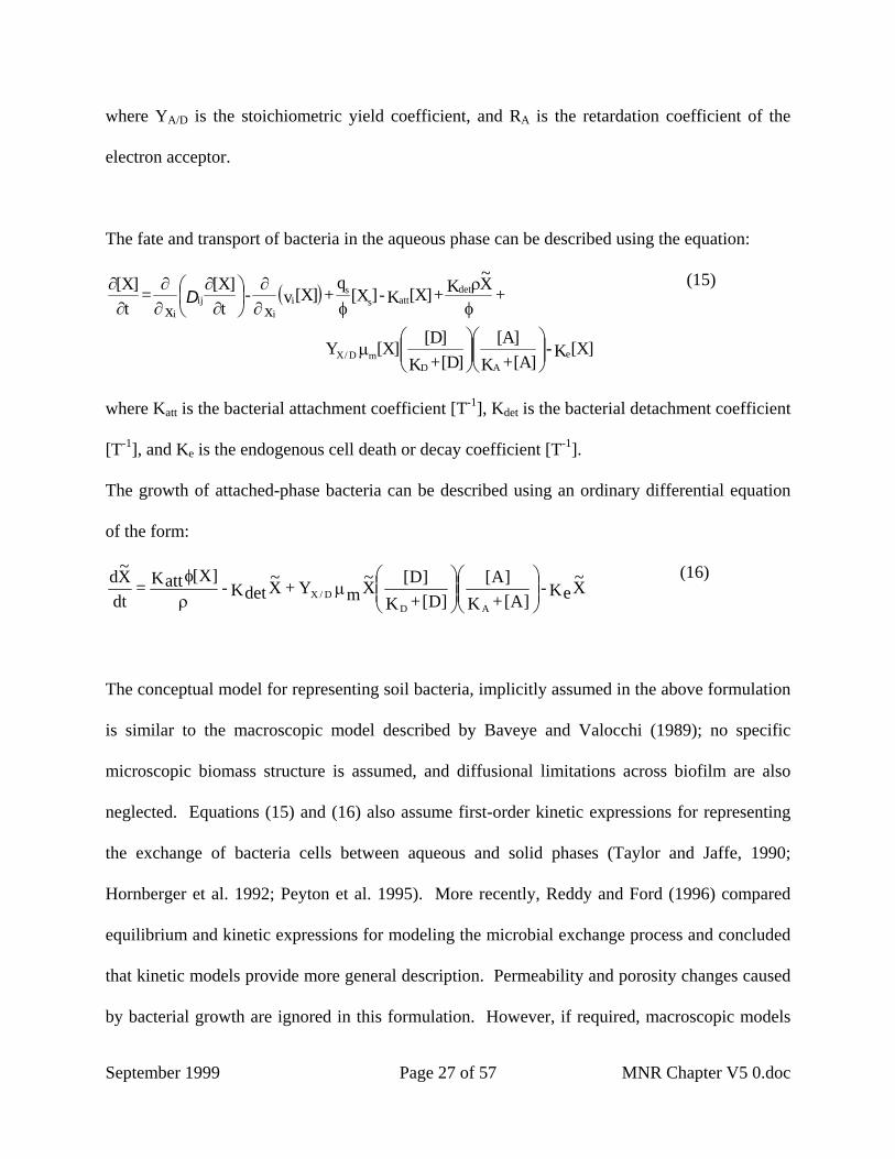
5.2.5 Modeling Natural Remediation of Chlorinated Solvents Plumes Waste sites where chlorinated solvent plumes are of primary concern commonly exist throughout


North America. Most of these chlorinated solvent plumes originated from waste disposal pits

where industrial solvents, such as PCE (tetrachloroethylene) and TCE (trichloroethylene) were

indiscriminately disposed. Recent demonstrations of natural degradation of petroleum

hydrocarbon, in virtually all groundwater systems, have raised the prospects that chlorinated

solvents might also be amenable for natural remediation. Wiedemeier et al. (1997) presented a

technical protocol that documents the conditions under which natural remediation of chlorinated

solvent may be feasible. The degree of natural remediation will obviously depend on the

biodegradation potential of the aquifer. Based on previous lab and field-scale results, they report

that the representative first-order biodegradation rates for chlorinated solvents in the presence of

aquifer materials may range from 0.00068 to 0.54 day-1 for PCE, 0.0001 to 0.021 day-1 for TCE,

0.00016 to 0.026 day-1 for DCE, and 0.0003 to 0.012 day-1 for VC (Wiedemeier et al. 1997).

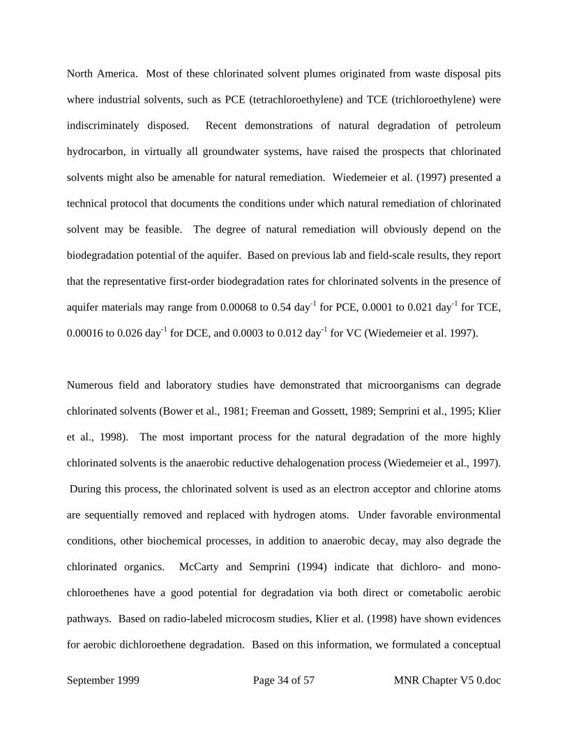
Numerous field and laboratory studies have demonstrated that microorganisms can degrade

chlorinated solvents (Bower et al., 1981; Freeman and Gossett, 1989; Semprini et al., 1995; Klier

et al., 1998). The most important process for the natural degradation of the more highly

chlorinated solvents is the anaerobic reductive dehalogenation process (Wiedemeier et al., 1997).

During this process, the chlorinated solvent is used as an electron acceptor and chlorine atoms

are sequentially removed and replaced with hydrogen atoms. Under favorable environmental

conditions, other biochemical processes, in addition to anaerobic decay, may also degrade the

chlorinated organics. McCarty and Semprini (1994) indicate that dichloro- and mono-

chloroethenes have a good potential for degradation via both direct or cometabolic aerobic

pathways. Based on radio-labeled microcosm studies, Klier et al. (1998) have shown evidences

for aerobic dichloroethene degradation. Based on this information, we formulated a conceptual


model for describing all biochemical reaction steps involved in dechlorination of various

chlorinated solvent chemicals. In this model, the degradation reactions are assumed to be

mediated by both aerobic and anaerobic dechlorination processes, as shown in Figure 6-8.

Assuming first-order biodegradation kinetics for every reaction step, the transport and

transformation of PCE, TCE, DCE, VC, ETH, and Cl can be simulated by solving the following

set of partial differential equations:

( ) ]PCE[K ]PCE[q

+x

]PCE[v- x

]PCE[D

x =

t]PCE[R Ps

s

i

i

jij

iP −

φ∂∂

⎟⎟⎠

⎞⎜⎜⎝

⎛

∂∂

∂∂

∂∂

(43)

( ) ]TCE[ K-]TCE[ K-]PCE[KY ]TCE[q

+x

]TCE[v- x

]TCE[D

x =

t]TCE[R 2T1TPP/Ts

s

i

i

jij

iT +

φ∂∂

⎟⎟⎠

⎞⎜⎜⎝

⎛

∂∂

∂∂

∂∂

(44)

( ) ]DCE[ K-]DCE[ K-]TCE[KY ]DCE[q

+x

]DCE[v- x

]DCE[D

x =

t]DCE[R 2D1DTT/Ds

s

i

i

jij

iD +

φ∂∂

⎟⎟⎠

⎞⎜⎜⎝

⎛

∂∂

∂∂

∂∂

(45)

( ) ]VC[ K-]VC[ K-]DCE[KY ]VC[q

+x

]VC[v- x

]VC[D

x =

t]VC[R 2V1V1DD/Vs

s

i

i

jij

iV +

φ∂∂

⎟⎟⎠

⎞⎜⎜⎝

⎛

∂∂

∂∂

∂∂

(46)

( ) ]ETH[ K-]ETH[ K-]VC[KY ]ETH[q

+x

]ETH[v- x

]ETH[D

x =

t]ETH[R 2E1E1VV/Es

s

i

i

jij

iE +

φ∂∂

⎟⎟⎠

⎞⎜⎜⎝

⎛

∂∂

∂∂

∂∂

(47)

( )

]VC[K2Y]DCE[K2Y]TCE[K2Y]VC[K1Y]DCE[K1Y

]TCE[K1Y]PCE[K1Y ]Cl[q

+x

]Cl[v- x

]Cl[D

x =

t]Cl[R

2VV/C

2DD/C2TT/C1VV/C1DD/C

1TT/C1PP/Css

i

i

jij

iC

+++++

++φ∂

∂⎟⎟⎠

⎞⎜⎜⎝

⎛

∂∂

∂∂

∂∂

(48)

where [PCE], [TCE], [DCE], [VC], [ETH], and [Cl] represent contaminant concentrations of

various species [mg/L]; KP, KT1, KD1, and KV1, and KE1 are first-order anaerobic degradation

rates [day-1]; KT2, KD2, and KV2, and KE2 are first-order aerobic degradation rates [day-1]; RP, RT,


RD, RV, RE, and RC are retardation factors; YT/P, YD/T, YV/D, and YE/V are chlorinated compound

yields under anaerobic reductive dechlorination conditions− their values are: 0.79, 0.74, 0.64 and

0.45, respectively; Y1C/P, Y1C/T, Y1C/D, and Y1C/V are yield values for chloride under anaerobic

conditions− their values are: 0.21, 0.27, 0.37, and 0.57, respectively; and Y2C/T, Y2C/D, and

Y2C/V are yield values for chloride under aerobic conditions− their values are: 0.81, 0.74, and

0.57, respectively. The yield values are estimated from the reaction stoichiometry and molecular

weights. The anaerobic degradation of one mole of PCE would yield one mole of TCE, therefore

YT/P = molecular weight of TCE/molecular weight of PCE (131.4/165.8 = 0.79). Note the

reaction models presented above assume that the biological degradation reactions only occur in

the aqueous phase, which is a conservative assumption.

All the reaction models described in this chapter for modeling natural remediation of fuel-

hydrocarbon and chlorinated solvent plumes are available in the RT3D code as pre-programmed

reaction modules. Several of these modules are field tested. In addition, several test example

data sets for applying these modules to predict plume migration scenarios, within the GMS

modeling environment, are documented in Clement and Jones (1998c).

Summary

Natural remediation is the reduction in contaminant concentration that naturally occurs as a

result of contaminant diffusion and dispersion, and as a result of natural degradation through

biotic and chemical reactions in the environment. This chapter describes important aspects of

the use and understanding of numerical models in the evaluation of natural remediation

scenarios. For this chapter, natural remediation models have been divided into two broad


classes; surface water models and groundwater models. Each environment, and thus model

type, has its own unique characteristics that control the rate of contaminant transport, dilution,

and degradation.

Surface water models have four components that must be integrated to produce an accurate

representation of contaminant fate and transport. These components are surface water

hydrodynamics, sediment transport, contaminant sorption/desorption processes, and contaminant

transformations (either biotic or chemical). The hydrodynamics of surface water systems

describe processes that affect the movement of water, and subsequently, the movement of

soluble and suspended contaminants from one location to another. In these surface water

systems, sediment transport is often a critical component of the model since many contaminants

are strongly sorbed to sediment particles. The deposition of sediment may significantly slow the

spreading of a contaminant. In contrast, resuspension events, such as floods or annual spring

runoff, may significantly increase, and may dominate, the contaminant transport properties in

surface systems. Contaminant sorption/desorption processes and transformation rates are often

very site and contaminant specific. Sorption/desorption processes control the distribution of a

contaminant between the solid and aqueous phases of the system. Transformation rates describe

the chemical or biological reactions that affect contaminant concentrations. Without laboratory

testing the sorption/desorption and reaction parameters are often difficult to quantify. Therefore

these processes, though very complex and the subject of significant research, are often modeled

as simple equilibrium and first order processes, respectively.

In contrast to surface water modeling, subsurface or groundwater modeling is slightly less


complex because of the significantly lower sediment transport load in aquifer systems and the

typically lower level of macrobiotic diversity found in aquifer systems. Natural remediation

modeling of groundwater systems requires knowledge of the subsurface hydrodynamics of

groundwater flow in response to natural hydrostatic gradients. Groundwater flow patterns can

also be influenced by wells used for irrigation or drinking water. Like surface water systems,

groundwater contaminant fate and transport is affected by contaminant sorption/desorption and

chemical and biotic transformations. Significant research has improved our understanding of the

chemical and biological processes that occur naturally in groundwater. These processes can

decrease contaminant concentrations and may eventually limit further spreading of contaminant

plumes.

Overall, modeling the natural remediation of contaminants in surface and subsurface water

systems has the potential to improve our estimates of the degradation rates and the extent of

spreading of contaminants released into our environment. In providing these estimates, the real

risks associated with natural remediation of environmental contaminants may be better balanced

against the costs of other remediation methods.

5.3 References

Ager DV. 1981. The nature of the stratigraphical record. New York, NY: John Wiley & Sons.

Ahlborg UG, Becking GC, Birnbaum LS, Brouwer A, Derks HJGM, Feeley M, Golor G,

Hanberg A, Larsen JC, Liem AKD, Safe SH, Schlatter C, Waern F, Younes M,

Yrjanheikki E. 1994. Toxic equivalency factors for dioxin-like PCBs - report on a WHO-

ECEH and IPCS consultation, December 1993. Chemosphere. 28:10-49.


Allison JA, Perdue EM. 1994. Modeling metal-humic interactions with MINTEQA2. In: Senesi

N, Miano TM, editors. Humic substances in the global environment and implications on

human health. Amsterdam: Elsevier. p927-942.

Ankley GT, Erickson R, Sheedy B, Kosian PA, Mattson V, Cox JS. 1997. Evaluation of models

for predicting the phototoxic potency of polycyclic aromatic hydrocarbons. Aquatic

Toxicology. 37:37-50.

Ambrose, Jr. RB, Wool TA, Martin JL. 1993. The water quality analysis simulation program,

WASP5, Part A: Model documentation. Center for Exposure Assessment Modeling

(CEAM), U.S. Environmental Protection Agency. Athens, GA. p.209

Barnthouse LW. 1993. Population-level effects. Boca Raton FL. Lewis Publishers.

Barnthouse LW, Suter G, Rosen A. 1990. Risks of toxic contaminants to exploited fish

populations: influence of life history, data uncertainty and exploitation intensity.

Environmental Toxicology and Chemistry. 9:297-311.

Bartell SM; Gardner RH, O'Neil RV. 1992. Ecological risk estimation. Boca Raton, FL. Lewis

Publishers.

Baveye, P. and Valocchi, V.A., 1989, An evaluation of mathematical models of the transport of

biologically reacting solutes in saturated soils and aquifers, Water Resources Research,

25, 1413-1421.

Barry, D.A., C.T., Miller, P.J., Culligan, K. Bajracharya, 1995, Split operator methods for

reactive chemical transport in groundwater, MODSIM95 conference proceedings.

Beamish FWH. 1964. Respiration of fishes with special emphasis on standard oxygen

consumption. Canadian Journal of Zoology. 42:177-188.

Bear, J., Hydraulics of groundwater, 1979, McGraw-Hill Book Co., Inc., New York, N.Y.

Bierman V; DePinto JV; Young TC; Rodgers PW; Martin SC; Raghunathan R, Hinz SC.

Development and validation of an integrated exposure model for toxic chemicals in


Green Bay, Lake Michigan. Prepared for EPA Large Lakes Research Station, Grosse Ile,

Michigan, Cooperative Agreement CR-814885.

Boese BL, Lee H, Echols S. 1997. Evaluation of a first-order model for the prediction of the

bioaccumulation of PCBs and DDT from sediment into the marine deposite-feeding clam

Macoma nasuta. Environmental Toxicology and Chemistry. 16:1545-1553.

Boething RS, Alexander M. 1979. Effect of concentration of organic chemicals on their

degradation by natural microbial communities. Appl. Environ. Microbiol.. 37:1211-1216.

Borden, R.C., Gomez, C.A., and Becker, M.T., 1995, Geochemical indicators of intrinsic

bioremediation, Ground Water, 33(2), 180-189.

Bower, E.J., Rittman, B.E., and McCarty, P.L., 1981, Anaerobic degradation of halogenated and

2-carbon organic compounds, Environmental Science and Technology, v. 15 (5), 596-

599.

Bradbury SP, Mekenyan OG, Ankley GT. 1998. The role of ligand flexibility in predicting

biological activity: structure – activity relationships for aryl hydrocarbon, estrogen, and

androgen receptor binding affinity. Environmental Toxicology and Chemistry. 17:15-25.

Brazner J, Heinis L, Jensen D. 1989. A littoral enclosure for replicated field experiments.


Calabrese EJ, Baldwin L. 1994. A toxicological basis to derive a generic interspecies uncertainty

factor. Environmental Health Perspectives. 102:14-17.

Campbell PGC, Tessier A. 1996. Ecotoxicology and metals in the aquatic environment:

geochemical aspects. In: Newman MC, Jagoe CH, editors. Ecotoxicology, A Hierarchical

Treatment. CRC Press.

Cardenas M, Lick W. 1996. Modeling the transport of sediments and hydrophobic contaminants

in the lower Saginaw River. J. Great Lakes Res. 22:669-682.

Caswell H. 1996. Demography meets ecotoxicology: untangling the population level effects of


toxic substances. In: Newman MC, Jagoe CH, editors. Ecotoxicology – A Hierarchical

Treatment. CRC Press.

Caswell H. 1989. Matrix population models: construction, analysis, and interpretation.

Sunderland, MA. Sinauer Associates.

Chapelle, F.H., McMahon, P.B., Dubrovsky, N,M., Fujii, R.F., Oaksford, E.T., and Vroblesky,

D.A., 1995, Deducing the distribution of terminal electron-accepting processes in

hydrologically diverse groundwater systems, Water Resources Research, 31(2), 359-371.

Cheng N-S. 1997. Simplified settling velocity formula for sediment particle. J. Hydr. Eng.

123:149-152.

Chilakapati, A., 1993, Numerical simulation of reactive flow and transport through the

subsurface, Ph.D. Thesis, Rice University, Houston, TX.

Chiang, C.Y., J.P. Salanitro, E.Y. Chai, J.D. Colthart, and C.L. Klein, 1989, Aerobic

biodegradation of benzene, toluene, and xylene in a sandy aquifer – Data analysis and

computer modeling, Ground Water, 27(6), 823-834.

Clark TP, Norstrom RJ, Fox GA, Woon HT. 1987. Dynamics of organochlorine compounds in

herring gulls (Larus argentatus): II. A two-compartment model and data for ten

compounds. Environmental Toxicology and Chemistry. 6:547-559.

Clement, T.P., Hooker, B.S., and Skeen, R.S., 1996a, Numerical modeling of biologically

reactive transport near a nutrient injection well, ASCE Journal of Environmental

Engineering Division, 122(9), 833-839.

Clement, T.P., Hooker, B.S., and Skeen, R.S., 1996b, Macroscopic models for predicting

changes in saturated porous media properties caused by microbial growth, Ground

Water, 34(5), 934-942.

Clement, T.P, Peyton, B.M., Skeen, R.S., Jennings, D.A., Petersen, J.N., 1997, Microbial growth

and transport in porous media under denitrification conditions: Experiment and


simulations, Journal of Contaminant Hydrology, 24, 269-285.

Clement, T.P, Peyton, B.M., Skeen, R.S., Jennings, D.A., Petersen, J.N., 1998, Modeling multi-

species reactive transport in groundwater, Groundwater Monitoring and Remediation

Journal, in press, Spring 98 issue.

Clement, T.P, 1998a, RT3D - A modular computer code for simulating reactive multi-species

transport in 3-Dimensional groundwater systems, Draft Report, Pacific Northwest

National Laboratory, PNNL-SA-28967, available at: http://etd.

pnl.gov:2080/bioprocess/rt3d.htm.

Clement, T.P., and Jones, N.L., RT3D tutorials for GMS users, 1998b, Pacific Northwest

National Laboratory, PNNL-11805, available at: http://etd.pnl.gov:

2080/bioprocess/rt3d.htm.

Connolly JP. 1991. Application of a food chain model to polychlorinated biphenyl contamination

of the lobster and winter flounder food chains in New Bedford Harbor. Environmental

Science & Technology. 25:760-770.

Connolly JP. 1997. Modeling the environmental fate and transport of metals. Society of

Environmental Toxicology and Chemistry (SETAC) Pellston Workshop on Reassessment

of Metals Criteria for Aquatic Life Protection; 1996 Feb 14-14; Pensacola, FL: SETAC

Pr. 114.

Connolly JP; Parkerton TF; Quadrini JD; Taylor ST, Thuman AJ. 1992. Development and

application of a model of PCBs in the Green Bay, Lake Michigan walleye and brown

trout and their food webs. Report for Large Lakes Research Station, U.S. EPA, Grosse

Ile, Michigan. Cooperative Agreement CR-815396.

Connolly JP, Zahakos HA, Benaman J, Ziegler CK, Rhea JR, Russell K. A model of PCB fate in

the Upper Hudson River. Submitted to Environ. Sci. Technol.

DeAngelis DL, Gross LJ. 1992. Individual-based models and approaches in ecology. New York

NY. Chapman & Hall.


de Blanc, P.C., D.C., McKinney, and G.E. Speitel, 1996, A 3-D flow and biodegradation model,

Proceeding of the ASCE conference on Non-aqueous phase liquid (NAPLs) in the

subsurface environment: Assessment and Remediation, Washington, D.C., p 478-489.

Dilks DW, Canale RP, Meier PG. 1992. Development of bayesian Monte-Carlo techniques for

water quality model uncertainty. Ecological Modelling 62:149-162.

Dilks DW, Helfand JS, Bierman Jr. VJ, Burkhard L. 1993. Field application of a steady-state

mass balance model for hydrophobic organic chemicals in an estuarine system. Wat. Sci.

Tech. 28:263-271.

DiToro DM, Parkerton TF. 1993. Uncertainty analysis methodology for Green Bay models.

Final Report to the US EPA Large Lakes Research Station, Grosse Ile, Michigan.

Cooperative Agreement CR-815397-01-0.

DiToro DM, Mahony JD, Hansen DJ, Scott KJ, Hicks MB, Mayr SM, Redmond MS. 1990.

Toxicity of cadmium in sediments: the role of acid volatile sulfide. Environmental

Toxicology and Chemistry. 9:1487-1502.

Domenico, P.A., and F.W., Schwartz, 1990, Physical and chemical hydrogeology, John Wiley &

Sons, New York.

Endicott D, Kreis RG, Mackelburg L, Kandt D. 1998. Modeling PCB bioaccumulation by the

zebra mussel (Dreissena polymorpha) in Saginaw Bay, Lake Huron. Journal of Great

Lakes Research. 24:411-426.

Erickson R, McKim J. 1990. A simple flow-limited model for exchange of organic chemicals at

fish gills. Environmental Toxicology and Chemistry. 9:159-165.

Evans D. 1984. Temperature independence of the annual cycle of standard metabolism in the

pumpkinseed. Transactions of the American Fisheries Society. 113:494-512.

Ferguson RI. 1987. Accuracy and precision of methods for estimating river loads. Earth Surf.

Proc. and Land. 12:95-104.


Freeman, D.L., and Gossett, J.M., 1989, Biological reductive dehalogenation of

tetrachloroethylene and trichloroethylene to etylene under methanogenic conditions,

Applied Environmental Microbiology, v. 55(4), 1009-1014.

Freeze, R.A., and J.A., Cherry, 1979, Groundwater, Prentice-Hall, Eaglewood Cliffs, New

Jersey.

Gabric AJ, Connell DW, Bell P. 1990. A kinetic model for bioconcentration of lipophilic

compounds by oligochaetes. Water Resources. 24:1225-1231.

Gill GA, Bloom NS, Cappellino S, Driscoll CT, Dobbs C, McShea L, Mason R, Rudd JWM.

1998. Sediment-water fluxes of mercury in Lavaca Bay, Texas. Submitted to Env. Sci.

Technol

Gilpin M, Hanski I. 1991. Metapopulation dynamics empirical and theoretical investigations.

San Diego, CA. Academic Press.

Glaser D, Connolly JP. 1994. Fish and wildlife toxicokinetic modeling and risk analysis.

Presentation at Annual Meeting of the Society for Risk Analysis; December 1994.

Glaser D, Connolly JP. 1995. Uncertainty in bioaccumulation modeling. Pages 8-49 through 8-

60 in Toxic Substances in Water Environments: Assessment and Control. Water

Environment Federation Specialty Conference; 1995.

Glaser D; Connolly JP, Bergoffen A. 1996. Population impacts of contaminants on the resident

bald eagles of the Lower Columbia River. Presentation at Society for Environmental

Toxicology and Chemistry Annual Meeting; November 1996.

Glaser D; Connolly JP, Haggard J. 1997. Development of a quantitative bioaccumulation model

for PCBs in fish from the Upper Hudson River. Presentation at Annual Meeting of the

Society for Environmental Toxicology and Chemistry; November 1997.

Gobas FAPC. 1993. A model for predicting the bioaccumulation of hydrophobic organic

chemicals in aquatic food-webs: application to Lake Ontario. Ecological Modeling .


69:1-17.

Gobas FAPC, McCorquodale JR, Haffner GD. 1993. Intestinal absorption and biomagnification

of organochlorines. Environmental Toxicology and Chemistry. 12:567-576.

Hallam T, Trawick T, Wolff W. 1996. Modeling effects of chemicals on a population:

application to a wading bird nesting colony. Ecological Modeling. 92:155-178.

Hanratty M, Liber K. 1996. Evaluation of model predictions of the persistence and ecological

effects of diflubenzuron in a littoral ecosystem. Ecological Modeling. 90:79-95.

Hanratty M, Stay F. 1994. Field evaluation of the littoral ecosystem risk assessment model's

predictions of the effects of chlorpyrifos. Journal of Applied Ecology. 31:439-453.

Hayton WL, Barron MG. 1990. Rate-limiting barriers to xenobiotic uptake by the Gill.


Hewett SJ. 1992. Bioenergetics model. University of Wisconsin Sea Grant Program.

Hindmarsh, A.C., and Petzold, L.R., 1995, Algorithm and software for ordinary differential

equations and differential algebraic equations, Part II: Higher order methods and software

packages, Computer in Physics, 9(2), 148-155.

Hornberger, G.M., Mills, A.L., and Herman, J.S., 1992, Bacterial transport in porous media:

Evaluation of a model using laboratory observations, Water Resources Research, 28,

915-938.

HydroQual, Inc. 1995. Addendum to Green Bay Final Report - Food chain model projections.

Report for Large Lakes Research Station, U.S. EPA, Grosse Ile, Michigan.

HydroQual, Inc. 1997. Southern California bight damage assessment food web/pathways study.

Report for the National Oceanic and Atmospheric Administration.


HydroQual, Inc. 1998. Development and application of a modeling framework to evaluate

hurricane impacts on surficial mercury concentrations in Lavaca Bay: Final Report to

Aluminum Company of America. Mahwah NJ.

Jepsen R, Roberts J, Lick W. 1997. Effects of bulk density on sediment erosion rates. Water, Air,

Soil Poll. 99:21-31.

Kaluarachchi, J., and J., Morshed, 1995, Critical assessment of the operator-splitting technique

in solving the advection-dispersion-reaction equation: 1. First-order reaction, Advances in

Water Resources, 18, 89-100.

Klier, N.J., R.J. West, and P.A. Donberg, 1998, Aerobic biodegradation of dichloroethylene in

subsurface soils, Chemosphere, in press.

Kolar C, Hudson P, Savino J. 1997. Conditions for the return and simulation of the recovery of

burrowing mayflies in Western Lake Erie. Ecological Applications. 7:665-676.

Konikow, L.F., and Bredehoeft, J.D., 1978, Computer model of two dimensional solute transport

and dispersion in groundwater, TWRI USGS Report I-19.15/5.

Landrum PF, Eadie B, Faust W. 1991. Toxicokinetics and toxicity of a mixture of sediment-

associated polycyclic aromatic hydrocarbons to the amphipod diporeia SP.


Lartiges SB, Garrigues PP. 1995. Degradation kinetics of organophosphorus and organonitrogen

pesticides in different waters under various environmental conditions. Envrion. Sci.

Technol. 29:1246-1254.

Leslie PH. 1945. On the use of matrices in certain population mathematics. Biometrika 33:183-

212.

Levin L, Caswell H, Bridges T, DiBacco C, Cabrera D, Plaia G. 1996. Demographic responses

of estuarine polychaetes to pollutants: life table response experiments. Ecological

Applications 6:1295-1313.


Levins R. 1975. Evolution in communities near equilibrium. In: Ecology and Evolution of

Communities. Cody, ML and Diamond, JM, editors. Cambridge MA. Belknap Press.

Limno-Tech, Inc., Menzie Cura & Associates, The Cadmus Group, Inc. 1996. Phase 2 Report -

further site characterization and analysis. Volume 2. Preliminary model calibration

report, Hudson River PCBs reassessment RI/FS. Prepared for the US EPA, Region II.

Loonen H, Muir DCG, Parsons JR, Govers HAJ. 1997. Bioaccumulation of polychlorinated

dibenzo-p-dioxins in sediments by oligochaetes: influence of exposure pathway and

contact time. Environ. Tox. Chem. 16:1518-1525.

Lotka AJ. 1925. Elements of mathematical biology. New York NY. Dover Publications, Inc.

Makay D, Yeun ATK. 1983. Mass transfer coefficient correlations for volatilization of organic

solutes from water. Environ. Sci. Technol. 17:211-217.

Malthus RT. 1978. An essay on the principle of population as it affects the future improvement

of society. Johnson, London.

Mazak EJ, MacIsaac HJ, Servos MR, Hesslein R. 1997. Influence of feeding habits on

organochlorine contaminant accumulation in waterfowl on the Great Lakes. Ecological

Applications. 7:1133-1143.

McCarty L, Mackay D. 1993. Enhancing ecotoxicological modeling and assessment.

Environmental Science & Technology. 27:1719-1728.

McCarty L, Mackay D, Smith A, Ozburn G, Dixon D. 1991. Interpreting aquatic toxicity

QSARs: the significance of toxicant body residues at the pharmacologic endpoint. The

Science of the Total Environment. 109/110:515-525.

McCarty L , Mackay D, Smith A, Ozburn G, Dixon D. 1992. Residue-based interpretation of

toxicity and bioconcentration QSARs from aquatic bioassays: neutral narcotic organics.


McCarty, P.L., and Semprini, L., 1994, Groundwater treatment for chlorinated solvents, In


Handbook of Bioremediation, Lewis Publishers, Florida.

McLachlan M, Mackay D, Jones PH. 1990. A conceptual model of organic chemical

volatilization at waterfalls. Environ. Sci. Technol. 24:252-257.

McLachlan M. 1994. Model of the fate of hydrophobic contaminants in cows. Environmental

Science & Technology. 28:2407-2414.

Molz, F.J., Widdowson, M.A., and Benefield, L.D., 1986, Simulation of microbial growth

dynamics coupled to nutrient oxygen transport in porous media, Water Resources

Research, 22, 1207-1216.

Munns W, Black D, Gleason T, Salomon K, Bengtson D, Guthjahr-Gobell R. 1997. Evaluation

of the effects of dioxin and PCBS on Fundulus heteroclitus populations using a modeling

approach. Environmental Toxicology and Chemistry. 16:1074-1081.

Newman MC, Dixon PM. 1996. Ecologically meaningful estimates of lethal effect in

individuals. In: Newman MC, Jagoe CH. Ecotoxicology: a hierarchical treatment. Boca

Raton FL. Lewis Publishers. p. 225-254.

Newman MC, Jagoe CH. 1996. Ecotoxicology: a hierarchical treatment. Boca Raton FL. Lewis

Publishers.

Newsted JL, Giesy JP, Ankley GT, Tillitt DE, Crawford RA, Gooch JW, Jones PD, Denison MS.

1995. Development of toxic equivalency factors for PCB congeners and the assessment

of TCDD and PCB mixtures in rainbow trout. Environmental Toxicology and Chemistry.

14:861-871.

Nichols JW, Larsen CP, McDonald ME, Niemi GJ, Ankley GT. 1995. Bioenergetics-based

model for accumulation of polychlorinated biphenyls by nestling tree

swallows/Tachycineta bicolor. Environmental Science & Technology. 29:604-612.

Norstrom RJ, McKinnon AE, DeFreita ASW. 1976. A bioenergetics-based model for pollutant

accumulation by fish. Simulation of PCB and methylmercury residue levels in Ottawa


River yellow perch (Perca flavescens). Jour. Fish. Res. Bd. Canada. 13:248-267.

O?Connor DJ, Connolly JP, Garland EJ. 1989. Mathematical models-fate, transport, and food

chain. In:Levin SA, Harwell MA, Kelly JR, Kimball KD, editors. Ecotoxicology:

problems and approaches. New York NY: Springer-Verlag. p. 221-243.

Opperhuizen A, Schrap SM. 1988. Uptake efficiencies of two polychlorobiphenyls in fish after

dietary exposure to five different concentrations. Chemosphere. 17:253-262.

Peyton, B.M., Skeen, R.S., Hooker, B.S., Lundman R.W., and Cunningham, A.B., 1995,

Evaluation of bacterial detachment rates in porous media, Applied Biochemistry and

Biotechnology, 51, 785-797.

Pignatello JJ, Xing, B. 1996. Mechanisms of slow sorption of organic chemicals to natural

particles. Environ. Sci. Technol. 30:1-11.

Puccia CJ, Levins R. 1985. Qualitative modeling of complex systems. Cambridge MA. Harvard

University Press.

Quantitative Environmental Analysis, LLC. 1999. PCBs in the Upper Hudson River: Report to

General Electric Company. Montvale NJ.

Raghunathan RJ, DePinto JV, Bierman Jr VJ, Rogers PJ, Young TC, Maritn SC, Zhang X. 1994.

Development of a toxic chemical dynamics model (GBTOX) for the Green Bay Mass

Balance Study: part two-model diagnosis and interpretation. J. Great Lakes Res.

Rathbun RE. 1990. Prediction of stream volatilization coefficients. J. Environ. Eng. 116:615-

631.

Reddy, H.L., and Ford, R.M., 1996, Analysis of biodegration and bacterial transport:

Comparison of models with kinetic and equilibrium bacterial adsorption, Journal of

Contaminant Hydrology, 22, 271-287.

Rice JA. 1981. Derivation and application of a bioenergetics model for largemouth bass

(micropterus salmoides). Ph.D. Thesis. University of Wisconsin, Madison, WI.


Rice, D.E., Grose, R.D., Michaelsen, J.C., Dooher, B.P., Macqueen, D.H., Cullen, S.J.,

Kastenberg, W.E., Everett, L.G., and Marino, M.S., 1995, California Leaking

Underground Fuel Tank (LUFT) historical case analyses, California State Water

Resources Publication, UCRL-AR-122207.

Riedel GF, Sanders JG, Osman RW. 1988. The effect of biological and physical disturbances on

the transport of arsenic from contaminated estuarine sediments. Est. Coastal Shelf Sci.

23:693-706.

Rifai, S.H., Bedient, P.B., Borden, R.C., and Haasbeek, J.F., 1987, BIOPLUME II - Computer

model of two-dimensional contaminant transport under the influence of oxygen limited

biodegradation in ground water, National Center for Ground Water Research, Rice

University.

Rifai, S.H., and Bedient, P.B., 1990, Comparison of biodegradation kinetics with an

instantaneous reaction model for groundwater, Water Resources Research, 637-655.

Rifai, S.H., Newell, C.J., Miller, R., Taffinder, S., and Rounsaville, M., 1998, BIOPLUME-III

reference here...***

Russom C, Bradbury S, Broderius S, Hammermeister D, Drummond R. 1997. Predicting modes

of toxic action from chemical structure: acute toxicity in the fathead minnow

(Pimephales promelas). Environmental Toxicology and Chemistry. 16:948-967.

Schecher WD, McAvoy DC. 1995. MINEQL+: a chemical equilibrium program for personal

computers. Hallowell ME: Environmental Research Software. Verson 3.01.

Schweiger, MB, Haggard, JG, Connolly JP. 1996. Comments of General Electric Company on

Phase 2 report - review copy: Further site characterization and analysis volume 2B -

Preliminary model calibration report Hudson River PCBs reassessment RI/FS. General

Electric Company, Albany NY.


Semprini, L., Kitanidis, P., Kampbell, D., and Wilson, J., 1995, Anaerobic transformation of

chlorinated aliphatic hydrocarbons in a sand aquifer based on spatial chemical

distribution, Water Resources Research, 31, 1051-1062.

Steefel, C.I., and Yabusaki, S.B., (1996), OS3D/GIMRT, Software for multicomponent-

multidimensional reactive transport, user manual and programmers guide, PNL-11166,

Pacific Northwest National Laboratory, Washington.

Suter GW. 1993. Ecological risk assessment. Boca Raton FL. Lewis Publishers.

Swackhamer DL, Skoglund RS. 1993. Bioaccumulation of PCBs by algae: kinetics versus

equilibrium. Environmental Toxicology and Chemistry. 12:831-838.

Taylor, S.W., and Jaffe, P.R., 1990, Biofilm growth and the related changes in the physical

properties of a porous medium, 1. Experimental investigations, Water Resources

Research, 26, 2153-2159.

Tell JG, Parkerton TF. 1997. A comparison of multi-medial models used in regulatory decision-

making. SAR QSAR Env. Res. 6:29-45.

Thomann RV, Connolly JP. 1984. Model of PCB in the Lake Michigan lake trout food chain.

Environmental Science & Technology. 18:65-71.

Thomann RV, Mueller JA, Winfield RP, Huang C-R. 1991. Model of fate and accumulation of

PCB homologues in Hudson Estuary. ASCE J. Environ. Engr. 117:161-178.

Thomann RV, Shkreli F, Harrison S. 1997. A pharmacokinetic model of cadmium in rainbow

trout. Environmental Toxicology and Chemistry. 16:2268-2774.

Thomas WA, McAnally WH. 1985. Open channel flow and sedimentation, TABS-2. U.S.A.E.

Waterways Experiment Station. Vicksburg MS. Instructional Report HL-85-1.

Tipping, E. 1994. WHAM - a chemical equilibrium model and computer code for waters,

sediments and soils incorporating a discrete site/electrostatic model of ion-binding by

humic substances. Computers & Geoscience 6:973-1023.


Tracey GA, Hansen DJ. 1996. Use of biota-sediment accumulation factors to assess similarity of

nonionic organic chemical exposure to benthically-coupled organisms of differing

trophic mode. Archives of Environmental Contamination and Toxicology. 30:467-475.

Tsai CH, Lick W. 1986. A portable device for measuring sediment resuspension. J. Great Lakes

Res. 12:314-321.

Tuljapurpkar S, Caswell H. 1997. Structured-population models in marine/terrestrial/and

freshwater systems. New York NY. Chapman & Hall.

[USEPA] United States Environmental Protection Agency. 1996. Phase 2 report - review copy:

Further site characterization and analysis volume 2B - Preliminary model calibration

report Hudson River PCBs reassessment RI/FS. New York NY: Region II.

[USEPA] United States Environmental Protection Agency. 1992. Framework for ecological risk

assessment. Washington D.C. US EPA.

[USEPA] United States Environmental Protection Agency. 1995. Great Lakes water quality

initiative criteria documents for the protection of wildlife. Washington D.C. US EPA.

Walker CH. 1987. Kinetic models for predicting bioaccumulation of pollutants in ecosystems.

Environmental Pollution. 44:227-240.

Wang XL, Ma YJ, Yu WJ, Geyer HJ. 1997. Two-compartment thermodynamic model for

bioconcentration of hydrophobic organic chemicals by alga: quantitative relationship

between bioconcentrations factor and surface area of marine algae or octanol/water

partition coefficient. Chemosphere. 35:1781-1797.

Ward CH. 1998. The role of ligand flexibility in predicting biological activity: structure-activity

relationships for aryl hydrocarbon, estrogen, and androgen receptor binding affinity.


Watanabe K, Bois F, Zeise L. 1992. Interspecies extrapolation: a reexamination of acute toxicity

data. Risk Analysis. 12:301-310.


[USEPA] U.S. Environmental Protection Agency. 1997. Phase 2 report – review copy: Further

site characterization and analysis volume 2C – Data evaluation and interpretation report

Hudson River PCBs reassessment RI/FS. New York, NY: Region II.

Valocchi, A.J. and M. Malmstead, 1992, Accuracy of operator-splitting for advection-dispersion-

reaction problems, Water Resources Research, 28, 1471-1476.

Velleux M, Endicott D, Steuer J, Jaeger S, Patterson D. 1995. Long-term simulation of PCB

export from the Fox River to Green Bay. J. Great Lakes Res. 21:359-372.

Voss, C.I., 1984, Two dimensional density dependent flow and transport of either dissolved

solute or thermal energy, USGS report.

Waddill, D.W., M.A., Widdowson, and J.S., Brauner, 1996, SEAM2D: A numerical model for

two-dimensional solute transport and sequential electron acceptor-based bioremediation

of LNAPL contaminated aquifers, Proceeding of the ASCE conference on Non-aqueous

phase liquid (NAPLs) in the subsurface environment: Assessment and Remediation,

Washington, D.C, November 12-14.

Walling DE, Webb BW. 1988. The reliability of rating curve estimates of suspended sediment

yield: some further considerations. In: Sediment Budgets. IAHS Pub. No. 174. P. 337-

350.

Walter, A.L., Frind, E.O., Blowes, D.W., Ptacek, C.J., and Molson, J.W., 1994, Modeling of

multicomponent reactive transport in groundwater 1. Model development and evaluation,

Water Resources Research, 30, 3137-3148.

Wiedemeier, T.H., Wilson, J.T., Kampbell, D.H., Miller, R.N., and Hansen, J., 1995, Technical

protocol for implementing intrinsic remediation with long-term monitoring for natural

attenuation of fuel contamination dissolved in groundwater, Volume 1 & 2, Air Force

Center for Environmental Excellence, Technology Transfer Division, Brooks AFB, San

Antonio, Texas.


Wiedemeier, T.H., M.A. Swanson, D.E. Moutoux, E.K. Gordon, J.T.Wilson, B.H. Wilson, D.H.

Kampbel, J. Hansen, and P. Haas, 1997, Technical protocol for evaluating natural

attenuation of chlorinated solvents in groundwater, Air Force Center for Environmental

Excellence, Technology Transfer Division, Brooks AFB, San Antonio, Texas.

Zheng, C., MT3D, 1990, A modular three-dimensional transport model for simulation of

advection, dispersion and chemical reactions of contaminants in groundwater systems,

U.S.E.P.A Report.

Ziegler, CK, Connolly JP. 1995. The impact of sediment transport processes on the fate of

hydrophobic organic chemicals in surface water systems. Water Environment Federation

Specialty Conference; 1995 May 14-17; Cincinnati, OH.

Ziegler CK, Israelsson PH, Connolly JP. Modeling of flood and long-term sediment transport

dynamics in Thompson Island Pool, Upper Hudson River. Submitted to ASCE J. Hyd. Engr.

Ziegler CK, Nisbet B. 1994. Fine-grained sediment transport in Pawtuxet River, Rhode Island.

ASCE J. Hyd. Engr. 120:561-576.

Ziegler CK, Nisbet B. 1995. Long-term simulation of fine-grained sediment transport in large

reservoir. ASCE J. Hydr. Engr. 121:773-781.

Zysset, A., Stauffer, F., and Dracos, T., 1994, Modeling of reactive groundwater transport

governed by biodegradation, Water Resources Research, 30, 2423-2434.


Figures


Mobile Components

Solve Advection for “m” mobile components

Solve Dispersion for “m” mobile components

Source/sink mixing for “m” mobile components

Solve coupled reactions for all “n” components

Immobile Components

No Advection

No Dispersion

No Source/sink

Numerical Solution Procedure...

Figure 6-8. Block Diagram Illustrating the Numerical Solution Scheme


EtheneVCDCE

CO2 + HCl

Cl

TCE

Cl Cl

PCE

Cl

Anaerobic AnaerobicAnaerobicAnaerobicAerobic

Aerobic

CO2 + 2HClCO2 + 3HCl

CH4Anaerobic

Aerobic

Aerobic

CO2

Figure 6-9. Conceptual biochemical model for biodegradation of chlorinated ethenes

(PCE=tetrachloroethene, TCE = trichloroethene, DCE = dichloroethene, VC= vinyl chloride)

AIR

WATER

BED

Hydrodynamics SedimentTransport

Physical/Chemical

Food ChainBioaccumulation

Hydrology Hydro-dynamics

DissolvedComponent

DissolvedOrganicCarbon

ParticulateComponent

SuspendedSolids

Settling

Scour

Volatilization

Groundwater AdvectionInterfacialBed Layer

IntermediateLayer

Deep Bed

ParticulateComponent

DissolvedComponent

DissolvedOrganicCarbon

Diffusion toDeep Bed

BenthicInvertebrates

Invertebrates ForageFish

PredatoryFish

Burial toDeep Bed

Diffusion

Partitioning

Partitioning

Partitioning

Predation

Dechlorination/Biodegradation

Humans &Wildlife

Biogeochemical Model Components

Date post:	26-Mar-2018
Category:	Documents
Upload:	vodan
View:	216 times
Download:	1 times

Modeling of Natural Remediation: Contaminant Fate … of Natural Remediation: Contaminant Fate and...

Documents