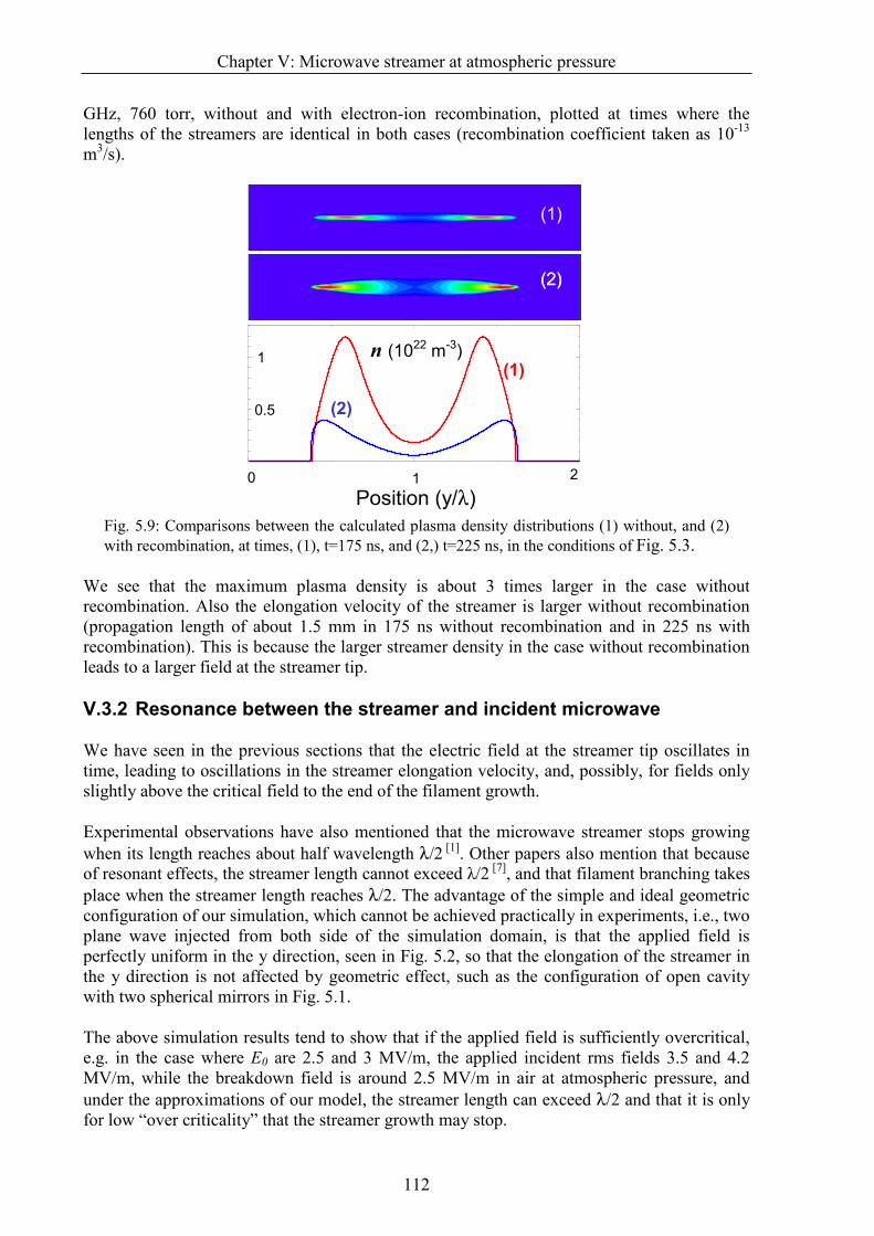
HAL Id: tel-00668934 https://tel.archives-ouvertes.fr/tel-00668934 Submitted on 10 Feb 2012 HAL is a multi-disciplinary open access archive for the deposit and dissemination of sci- entific research documents, whether they are pub- lished or not. The documents may come from teaching and research institutions in France or abroad, or from public or private research centers. L’archive ouverte pluridisciplinaire HAL, est destinée au dépôt et à la diffusion de documents scientifiques de niveau recherche, publiés ou non, émanant des établissements d’enseignement et de recherche français ou étrangers, des laboratoires publics ou privés. Modeling of plasma dynamics and pattern formation during high pressure microwave breakdown in air Guo-Qiang Zhu To cite this version: Guo-Qiang Zhu. Modeling of plasma dynamics and pattern formation during high pressure microwave breakdown in air. Plasmas. Université Paul Sabatier - Toulouse III, 2012. English. tel-00668934
Transcript
HAL Id: tel-00668934https://tel.archives-ouvertes.fr/tel-00668934
Submitted on 10 Feb 2012
HAL is a multi-disciplinary open accessarchive for the deposit and dissemination of sci-entific research documents, whether they are pub-lished or not. The documents may come fromteaching and research institutions in France orabroad, or from public or private research centers.
L’archive ouverte pluridisciplinaire HAL, estdestinée au dépôt et à la diffusion de documentsscientifiques de niveau recherche, publiés ou non,émanant des établissements d’enseignement et derecherche français ou étrangers, des laboratoirespublics ou privés.
Modeling of plasma dynamics and pattern formationduring high pressure microwave breakdown in air
Guo-Qiang Zhu
To cite this version:Guo-Qiang Zhu. Modeling of plasma dynamics and pattern formation during high pressure microwavebreakdown in air. Plasmas. Université Paul Sabatier - Toulouse III, 2012. English. �tel-00668934�
My sincere appreciation goes out to my advisor Jean-Pierre Boeuf who provided the opportunity of working on the present subject at LAPLACE/GREPHE. Thank you for leading me to this magical plasma world and guiding me during the research work, thank you for sharing the skill in paper writing and presentation, and for your thoughtfulness, kindness, and inspiration. In a word, I do not think I could ever find a better advisor than you for me.
My appreciation also goes to other GREPHE members, Leanne Pitchford, Laurent Garrigues and Garjan Hagelarr, thank you for the great help both in the research work and daily life during the past three years.
The great appreciation goes to Professor Ana Lacoste and Professor Khaled Hassouni, thank you for reporting my thesis work.
I would show my special appreciation to the post-doctroal and co-worker, Bhaskar Chaudhury, thank you for the many many helpful discussions and your parallel results, and for correcting the mistakes in my manuscript.
Thanks Nicolas and Noureddine, I really enjoy the lab life we shared together, and thank you for the helpful daily discussions and the great help in French language.
A big thank you goes to my friends, those that I made in Toulouse, at LAPLACE, Philippe, Jonathan, Juslan, Elisa, Sédiré, Amine, José, Cherif, Benoit, Namjun, Raja, Thiery and Thomas. Thanks Yu, Siyuan, Zhen, Yuan, Yanling, Xiao Yu, Zhongxun, Chao, Yunhui, Lanlan and all the other Chinese friends of mine, thank you for making me not feel lonely in a foreign country.
Thanks my grandparents and parents, sister and bothers. Thank you for the warm and rich home life and the great support you giving to me.
Thanks my beloved wife, thank you for the company and encouragement during the difficulte times, thank you making me feel be loved so much. Also thanks my to be-borned baby for the great happiness you bring to me.
My final appreciation goes to China Scholarship Council for the financial support in the past three years, and PLASMAX project for the opportunity to work on microwave breakdown.
Acknowledgements
ii
—— To my grandfather, and hope him enjoying happiness and peace in another world.
—— 献给我深爱的祖父,愿他在天国永享幸福和安宁。
Table of contents
iii
Table of contents
ACKNOWLEDGEMENTS ........................................................................................................ I
TABLE OF CONTENTS ........................................................................................................... III
GENERAL INTRODUCTION .................................................................................. 1
Gas discharges have been observed and studied for more than 200 years. They can be observed in nature as well as in laboratory experiments. Historically, the term gas discharge refers to the discharge of a plate capacitor through an air gap, while now this term is used for any electric current flowing through an ionized gas. Microwave discharges have been investigated relatively more recently than other types of discharges since they were first systematically studied in the late 1940s. The free located microwave discharges that are considered in this thesis work were first observed during the 1980s, after the gyrotrons became available for laboratory experiments. In present days the elementary processes of gas discharges are generally well understood, but the complex and non-linear interaction between charged particle transport, reactions, and self-consistent fields is still the subject of intense research in the context of very different applications. The increasing development of sophisticated diagnostic tools and availability of powerful and low cost computing resources lead to continuous progress in the understanding and control of the complex mechanisms taking place in gas discharges.
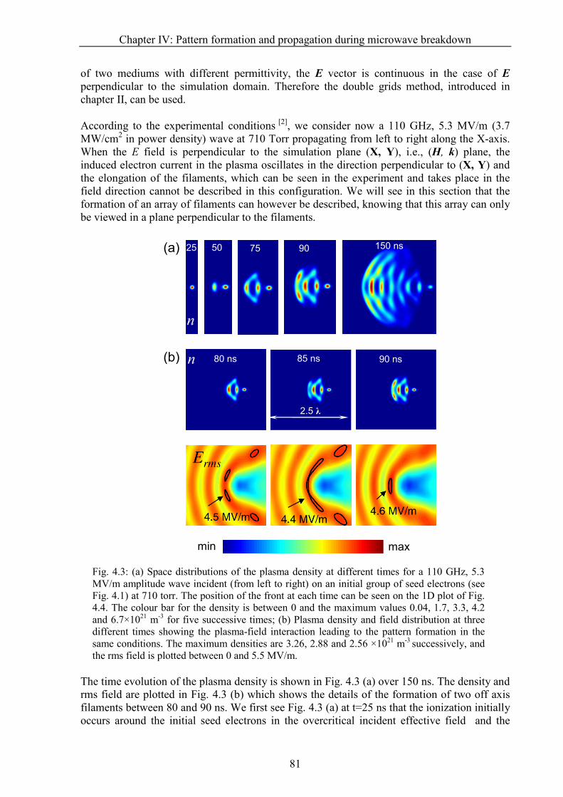
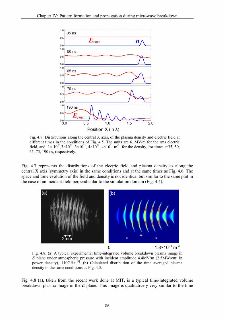
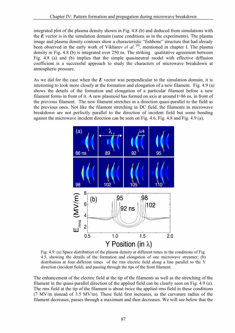
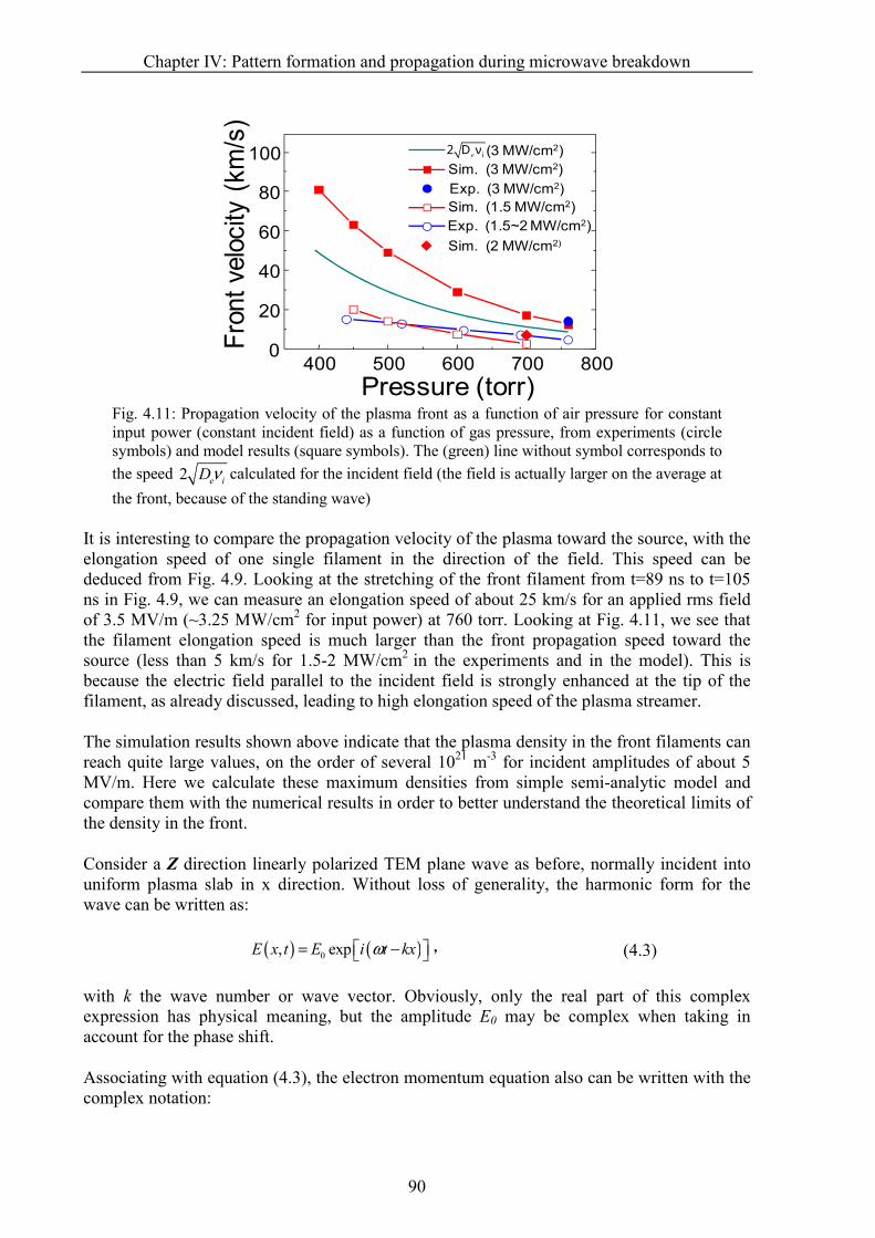
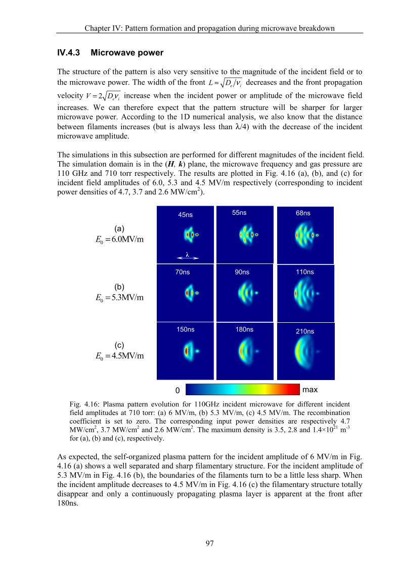
The early experimental and theoretical studies of microwave discharges in free space were focused on the determination of the breakdown field as a function of several parameters such as pressure, frequency, and pulse duration. In contrast to breakdown under DC fields at atmospheric pressure, which has led to a number of experimental, theoretical, and numerical studies (avalanche to streamer transition, streamer development, streamer to spark transition, filament branching …), microwave breakdown at high pressure and the plasma dynamics after breakdown have received relatively less attention. This is due to the fact that microwave sources able to trigger breakdown in air at atmospheric pressure are not as common and available as high voltage DC voltage sources. The plasma dynamics after microwave breakdown at high pressure however exhibits very spectacular features such as the development of filamentary structures that propagate toward the microwave source and form complex network. Such features have been observed and reported in Russia in the 1980s. Although the basic physics that determines the plasma dynamics after breakdown and the associated models equations are known, there has been no systematic attempt (at least not reported in the English literature) at solving numerically the equations describing these phenomena. Recently, microwave experiments in atmospheric pressure air performed at MIT have revealed in a very clear way, using fast imaging techniques, the formation and self-organization of filamentary plasma array propagating toward the microwave source. These MIT experiments have motivated the work presented in this thesis, the objective being to define the simplest possible physical model able to describe and reproduce the experimental observations.
In this thesis work we have developed a model for the microwave–atmospheric plasma interaction based on solutions of Maxwell’s equations for microwave coupled with plasma model equations describing plasma growth and transport in the microwave field. The plasma model is kept as simple as possible and consists in a diffusion-ionization-attachment-recombination equation for the quasineutral plasma density associated with a simplified electron momentum transfer equation to calculate the electron current density. The Maxwell-plasma interaction in these conditions can be summarized as follows: electromagnetic field
General introduction
2
“sees” the plasma through the electron current density in Maxwell’s equations while the plasma is sensitive to the electromagnetic field through the ionization frequency in the density equation (this interaction is strongly non-linear). An important aspect of the plasma density equation was to find a proper way to describe plasma diffusion. This is because, as we will see along this thesis, the expansion of the quasineutral, collisional plasma under these conditions is mainly related to a diffusion-ionization mechanism at the plasma edge. The value that must be taken for the diffusion coefficient at the plasma edge (ambipolar or free?) is therefore an issue. We show in this thesis that if a proper form of the diffusion is included in the density equation, this simple model is able to reproduce a number of experimental features such as the formation of self-organized filamentary structures and the propagation velocity.
Simulations performed in one and two dimensions with a linearly polarized TEM (transverse-electric-magnetic) plane wave as in the experiments can reproduce the experimental observations and allow a clear understanding of the complex plasma pattern formation and the jump-like plasma front propagation. New filaments develop ahead of previous ones because of diffusion-ionization mechanisms in the standing wave field that develop in front of the high density filament. The filaments stretch in a direction parallel to the incident electric field because of polarization effects, in a way that is very similar to DC streamers (intense field at the streamer tips, decrease of the field inside the plasma filament). We also provide a detailed description of the development of an isolated streamer and show evidence of the existence of resonant effects due to the fact that a streamer with sufficient density behaves like a small antenna.
The manuscript is organized in 5 chapters as follows: The first chapter presents an introduction to microwave breakdown starting with a brief review of the gas discharge development history, a description of possible applications and a brief literature overview. In the second chapter a closed physical model for the microwave breakdown in high pressure air is established and the corresponding numerical schemes are presented. The expression of the effective diffusion coefficient describing the diffusion transition at plasma front is also derived in this chapter. The third chapter is divided into two sections: in the first section the numerical validation of the effective diffusion coefficient is performed by comparing the simulation results with the ‘more exact’ drift-diffusion-Poisson model, in the second section the plasma pattern formation is studied by coupling Maxwell’s equations and plasma equations in 1D, and the influence of recombination, pressure and negative ions is also discussed. The fourth chapter presents the 2D simulations in both (E, k) plane and (H, k) plane (k is the wave vector). The detailed dynamics of the self-organized pattern formation are shown and discussed in this chapter, and comparisons between the simulation results and the experimental observations under similar conditions are performed. The elongation of an isolated plasma filament (microwave streamer) formed in the standing wave at the intersection of two incident waves with opposed wave vectors is studied in the fifth chapter.
This thesis work has been done in the GREPHE (Groupe de Recherche Energétique, Plasma, Hors-Equilibre) group of LAPLACE (LAboratoire PLAsma et Conversion d’Energie) in the frame of the PLASMAX project supported by the RTRA STAE “Fondation de Coopération Scientifique Sciences et Technologies pour l'Aéronautique et l'Espace”. One of the goals of the PLASMAX project was the development of physical models and numerical tools to study the interaction of microwave field and plasmas at high pressure under conditions that could be relevant to aerodynamic and aerospace applications (breakdown next to antenna, protection against high power microwave, flow control, shockwave mitigation, and ignition control). The parallelized code for 2D simulations in (E, k) plane is developed by B. Chaudhury, post-doctoral fellow in GREPHE in the frame of the PLASMAX project.
Chapter I: Introduction – Microwave breakdown
3
Chapter I
Introduction - Microwave breakdown
Chapter I: Introduction – Microwave breakdown
4
Chapter I: Introduction – Microwave breakdown
5
I.1 Gas discharge and microwave breakdown
The work performed in this thesis is the modeling and simulation on microwave breakdown discharge under atmospheric pressure. Microwave breakdown, which was first systematically studied in the late 1940s [1], is not a ‘new’ research subject in gas discharge but recent advances in microwave sources, plasma diagnostic techniques, numerical simulation and computing power have allowed significant progress in the understanding of plasma formation during microwave breakdown. In the following we will introduce the subject by giving a brief review of the development of gas discharge firstly.
I.1.1 Brief history of the gas discharge
Gas discharge is a basic physical phenomenon in the nature. Leaving lightning alone, the first observation on man-made electric discharges can date back to 17th century, when the researcher saw the friction charged insulated conductors lose their charge. Coulomb proved experimentally in 1785 that charge leaks through air. We understand now that the cause of leakage is the non-self-sustaining discharge.
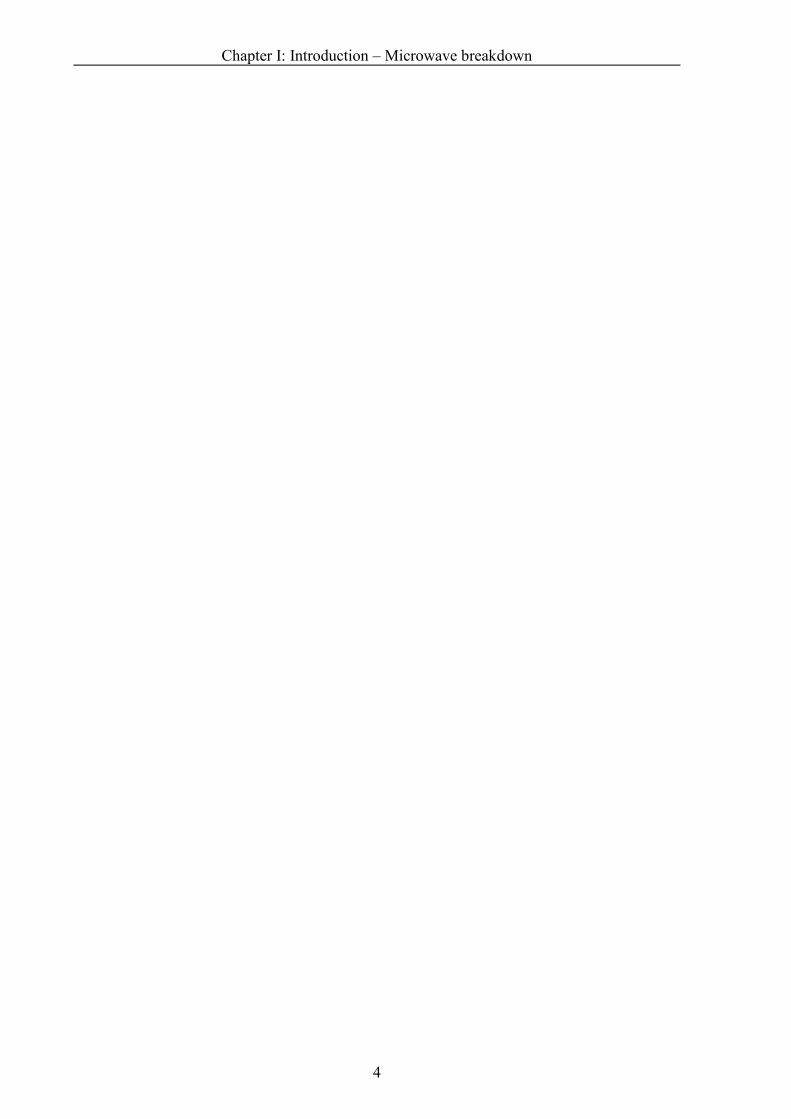
After the first battery (the voltaic pile) was developed by A. Volta in 1800, the sufficiently powerful electric batteries were developed, and this allows the discovery of arc discharge which was first reported by V. V. Petrov in Russia in 1803. Several years later Humphrey Davy in Britain produced and studied the arc in air. This type of discharge became known as ‘arc’ because its bright horizontal column between two electrodes bends up and arches the middle owing to the Archimedes’s force. The glow discharge was first discovered and studied by Faraday in thirties of 19th century. Faraday worked with tubes evacuated to a pressure about 1 torr and applied voltage up to 1000V. In 1855, with the work of Heinrich Geissler, the first evacuated (~103 Pa) glass tubes (seen in Fig. 1.1) became available for scientific research and made it easy to study discharges in a more controlled environment.
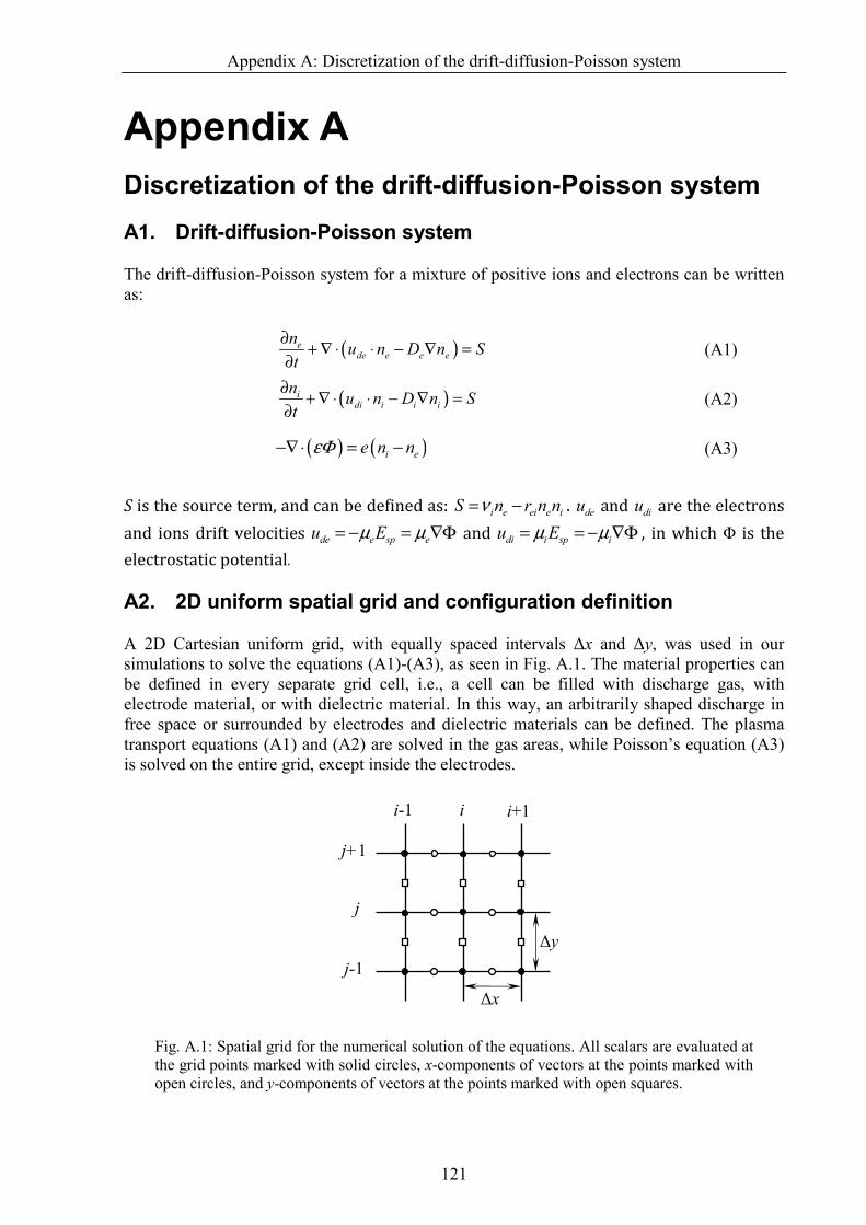
Fig. 1.1: Classical experimental setup for the typical gas discharge tube
Most of the observations and studies of gas discharges in the late 19th and early 20th centuries were performed in the context of atomic physics research. After William Crookes’ cathode ray experiments, which were also preformed with glass discharge tubes, and J. J. Thomson’s measurements of the e/m ratio, it became clear that the current in gases is mostly carried by electrons. A great deal of information on elementary processes involving electrons, ions, atoms, and light fields was obtained by studying phenomena in gas discharge tubes.
R
anode cathode
- +
Chapter I: Introduction – Microwave breakdown
6
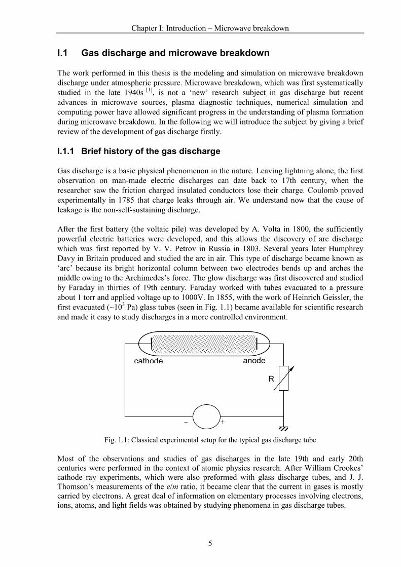
In 1889 [2], Friedrich Paschen published his work in which he investigated the minimum potential that is necessary to generate a spark in the gap between the two electrodes in gas discharge tubes. Curves of this potential as a function of pressure and the gap distance are nowadays called Paschen curves (see Fig. 1.2 (a)).
At the beginning of 1900 [3], J. S. E. Townsend proposed the theory of ionization by collision to explain the development of currents in gases, by which many phenomena in connection with the discharge through gas can be explained, including Paschen’s observations. He introduced a coefficient α to describe the average number of electrons produced by one electron moving through a unit length of centimetre in gas. This so-called ionization coefficient is widely used in the study of various discharge phenomena, including the work performed in this thesis. Numerous experimental results were gradually accumulated on cross sections of various electron-atom collisions, drift velocities of electrons and ions, their recombination coefficients, etc. These works built the foundations of the current reference sources, without which no research in discharge physics would be possible. The concept of plasma was first introduced by I. Langmuir and L. Tonks in 1928 [4], [5]. Langmuir also made many important contributions to the physics of gas discharge, including probe techniques [6] of plasma diagnostics.
Fig. 1.2: (a) The Paschen curves for different gases [7], the minimum in the curve is called Stolevtov’s point; (b) the dependence of α/p on the reduced electric field E/p for various gases [8].
Regarding different frequency ranges, the development of field generators and the research into the discharges they produce followed the order of increasing frequencies. Radio frequency (RF) discharges were first observed by N. Tesla in 1891 and the inductively coupled RF discharges up to the power of tens of kW were obtained by G. I. Babat in Leningrad around 1940. The progress in radar technology drew attention to phenomena in
microwave field. S. C. Brown et al., began the systematic studies of microwave discharges
in the late 1940s [1]. Discharges in the optical frequency range were realized after the advent
of the laser and being achieved successfully in 1963 [9]. The physical interactions during microwave and optical discharges is more complex than the discharges in constant electric fields, which have been studied for more than 200 years, and the new features are still being discovered continually in now days.
In the present day the elementary processes of gas discharge are generally well understood. However, the question of how these processes interact to determine the more macroscopic phenomena in gas discharges is what drives researches. The many possible configurations, the
(b) (a)
Chapter I: Introduction – Microwave breakdown
7
interactions of the discharge with itself and its surroundings, both at microscopic and macroscopic length scales, all give rise to a myriad of applications of gas discharges. Among these are lighting, material processing, propulsion and chemical analysis. New types of discharges keep emerging and give rise to new applications and technologies.
I.1.2 Classification of gas discharge
As can be seen in the brief review, the gas discharge (plasma) is a wide subject. Nevertheless, it can be classified with the terminology typical of this field.
There is a variety of known discharge types. The parameters characterizing the gas discharge are the gas type, ambient pressure and temperature, spatial dimensions and the shape of the discharge region, presence and composition of electrodes and boundaries, the kind of energy supply, presence of external magnetic field, etc. Internally, gas discharges are characterized by the electric field and its homogeneity, the ionization rate, energy distribution of particles, spatial distribution of charge carriers, dominant processes in the plasma, etc.
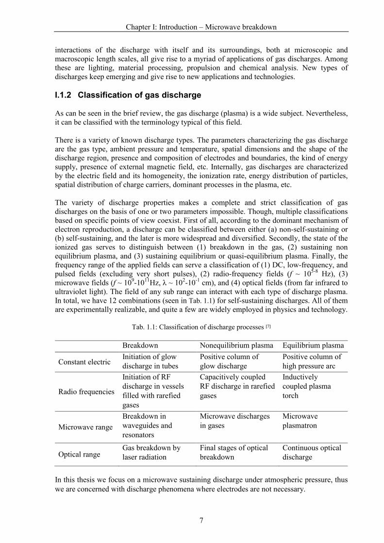
The variety of discharge properties makes a complete and strict classification of gas discharges on the basis of one or two parameters impossible. Though, multiple classifications based on specific points of view coexist. First of all, according to the dominant mechanism of electron reproduction, a discharge can be classified between either (a) non-self-sustaining or (b) self-sustaining, and the later is more widespread and diversified. Secondly, the state of the ionized gas serves to distinguish between (1) breakdown in the gas, (2) sustaining non equilibrium plasma, and (3) sustaining equilibrium or quasi-equilibrium plasma. Finally, the frequency range of the applied fields can serve a classification of (1) DC, low-frequency, and pulsed fields (excluding very short pulses), (2) radio-frequency fields (f ~ 105-8 Hz), (3) microwave fields (f ~ 109-1011Hz, λ ~ 102-10-1 cm), and (4) optical fields (from far infrared to ultraviolet light). The field of any sub range can interact with each type of discharge plasma. In total, we have 12 combinations (seen in Tab. 1.1) for self-sustaining discharges. All of them are experimentally realizable, and quite a few are widely employed in physics and technology.
Tab. 1.1: Classification of discharge processes [7]
Constant electric Initiation of glow discharge in tubes
Positive column of glow discharge
Positive column of high pressure arc
Radio frequencies
Initiation of RF discharge in vessels filled with rarefied gases
Capacitively coupled RF discharge in rarefied gases
Inductively coupled plasma torch
Microwave range
Breakdown in waveguides and resonators
Microwave discharges in gases
Microwave plasmatron
Optical range Gas breakdown by laser radiation
Final stages of optical breakdown
Continuous optical discharge
In this thesis we focus on a microwave sustaining discharge under atmospheric pressure, thus we are concerned with discharge phenomena where electrodes are not necessary.
Chapter I: Introduction – Microwave breakdown
8
I.1.3 Microwave discharge and applications
In a microwave discharge, free electrons are accelerated by the microwave electromagnetic field, which enables them to ionize the natural gas particles in collisions and ignite and sustain a plasma.
The discharge phenomenon in microwave field was first extensively investigated in the late 1940s in order to solve the problem of discharge formation within a waveguide in a radar system. The work was mainly performed by S. C. Brown, A. D. MacDonald et al. at Research Laboratory of Electronics (RLE) in MIT, and a series of quarterly progress reports and papers on this subject were presented in the following decade. This early work was summarized by MacDonald in ‘Microwave Breakdown in Gases’ published in 1966 [1].
After that, benefiting from the rapid development of the High Power Microwave (HPM) technology, the studies of microwave breakdown and “Microwave Induced Plasmas” (MIPs) were carried out extensively. These works were performed over a wide range of conditions, i.e., a frequency ranging from several hundred MHz to terahertz [10], a pressure changing from less than 0.1 Pascal to a few atmospheres, a power between a few Watts and several MWs, sustaining in both noble and molecular gases, with or without external magnetic field. Depending on the different operating conditions and different discharge mechanisms, the MIPs also can be classified into several different types, e.g. Electron Cyclotron Resonance (ECR) plasmas, cavity induced plasmas, free expanding atmospheric plasma torches, Surface Wave Discharges (SWD), etc. All these MIPs have been widely used in various fields, such as Plasma Enhanced Chemical Vapor Deposition (PECVD), plasma sterilization, and space propulsion [11].
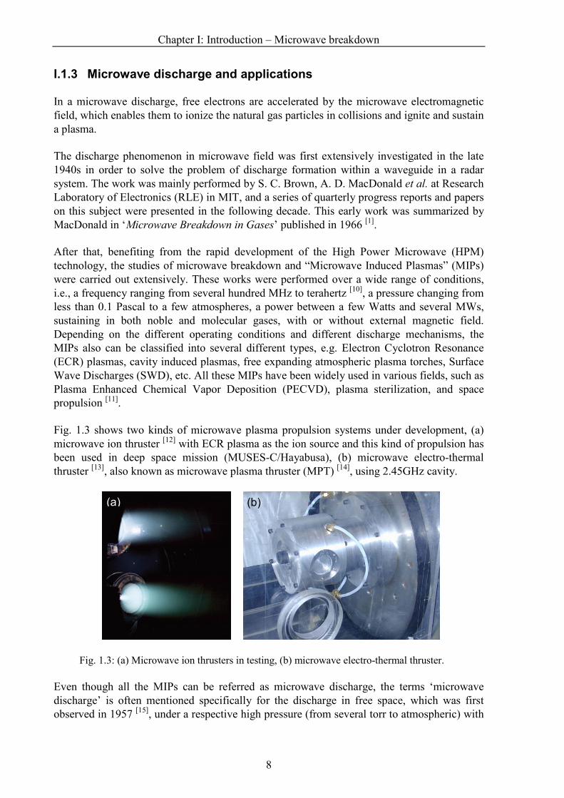
Fig. 1.3 shows two kinds of microwave plasma propulsion systems under development, (a) microwave ion thruster [12] with ECR plasma as the ion source and this kind of propulsion has been used in deep space mission (MUSES-C/Hayabusa), (b) microwave electro-thermal thruster [13], also known as microwave plasma thruster (MPT) [14], using 2.45GHz cavity.
Fig. 1.3: (a) Microwave ion thrusters in testing, (b) microwave electro-thermal thruster.
Even though all the MIPs can be referred as microwave discharge, the terms ‘microwave discharge’ is often mentioned specifically for the discharge in free space, which was first observed in 1957 [15], under a respective high pressure (from several torr to atmospheric) with
(a) (b)
Chapter I: Introduction – Microwave breakdown
9
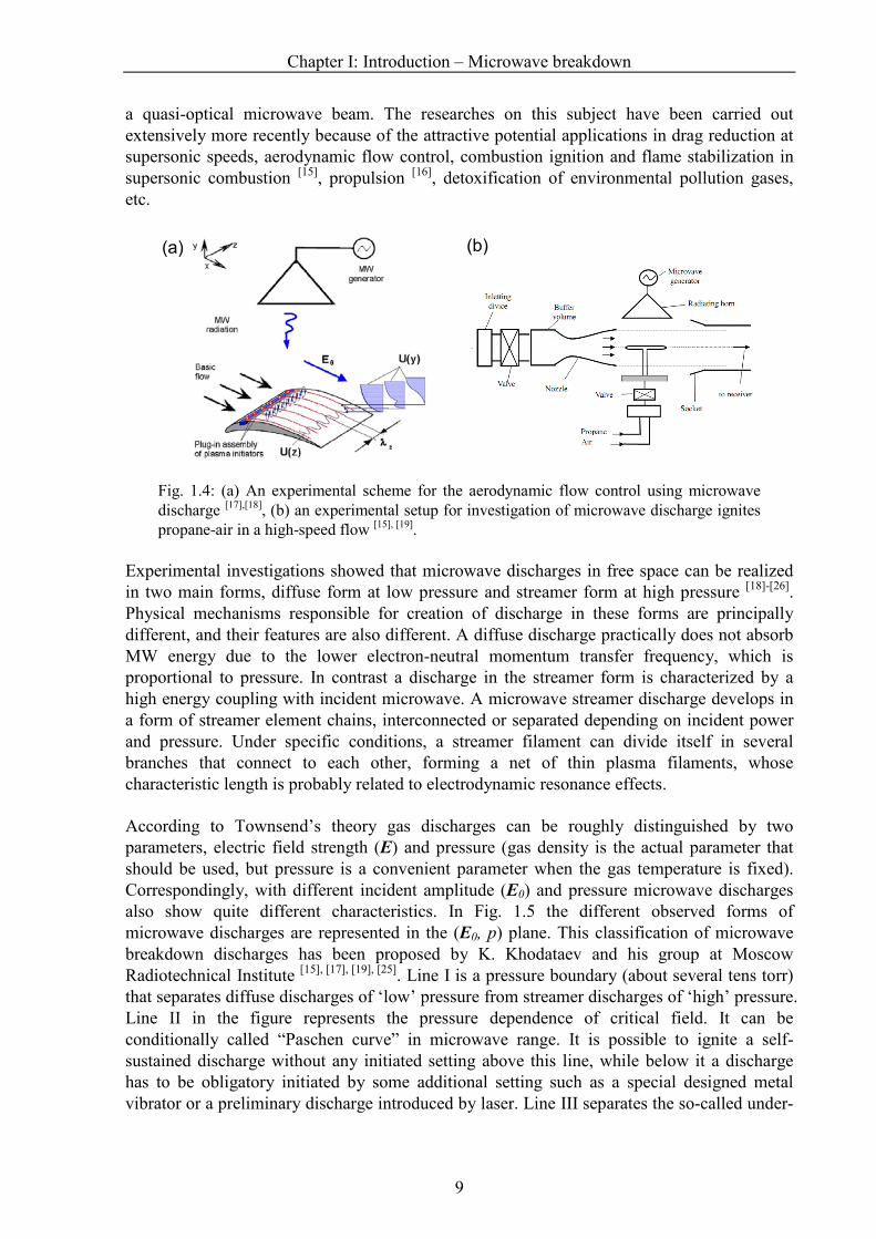
a quasi-optical microwave beam. The researches on this subject have been carried out extensively more recently because of the attractive potential applications in drag reduction at supersonic speeds, aerodynamic flow control, combustion ignition and flame stabilization in supersonic combustion [15], propulsion [16], detoxification of environmental pollution gases, etc.
Fig. 1.4: (a) An experimental scheme for the aerodynamic flow control using microwave discharge [17],[18], (b) an experimental setup for investigation of microwave discharge ignites propane-air in a high-speed flow [15], [19].
Experimental investigations showed that microwave discharges in free space can be realized in two main forms, diffuse form at low pressure and streamer form at high pressure [18]-[26]. Physical mechanisms responsible for creation of discharge in these forms are principally different, and their features are also different. A diffuse discharge practically does not absorb MW energy due to the lower electron-neutral momentum transfer frequency, which is proportional to pressure. In contrast a discharge in the streamer form is characterized by a high energy coupling with incident microwave. A microwave streamer discharge develops in a form of streamer element chains, interconnected or separated depending on incident power and pressure. Under specific conditions, a streamer filament can divide itself in several branches that connect to each other, forming a net of thin plasma filaments, whose characteristic length is probably related to electrodynamic resonance effects.
According to Townsend’s theory gas discharges can be roughly distinguished by two parameters, electric field strength (E) and pressure (gas density is the actual parameter that should be used, but pressure is a convenient parameter when the gas temperature is fixed). Correspondingly, with different incident amplitude (E0) and pressure microwave discharges also show quite different characteristics. In Fig. 1.5 the different observed forms of microwave discharges are represented in the (E0, p) plane. This classification of microwave breakdown discharges has been proposed by K. Khodataev and his group at Moscow Radiotechnical Institute [15], [17], [19], [25]. Line I is a pressure boundary (about several tens torr) that separates diffuse discharges of ‘low’ pressure from streamer discharges of ‘high’ pressure. Line II in the figure represents the pressure dependence of critical field. It can be conditionally called “Paschen curve” in microwave range. It is possible to ignite a self-sustained discharge without any initiated setting above this line, while below it a discharge has to be obligatory initiated by some additional setting such as a special designed metal vibrator or a preliminary discharge introduced by laser. Line III separates the so-called under-
(a) (b)
Chapter I: Introduction – Microwave breakdown
10
critical and deeply under-critical discharge forms of obligatory initiated discharges. Both numerical and experimental investigations have shown that in the under-critical and deeply under-critical discharges the local field induced at the ends of the metallic initiator is significantly enhanced to a level above the critical value. The typical images for discharges in each existence fields also are presented on Fig. 1.5. One can see that the difference between the under-critical and deeply under-critical discharges is that the streamers remain “attached” to the initiator for deeply under-critical case. The diffuse discharge plasma in the under-critical region also remains attached to the initiator.
Fig. 1.5: Microwave discharge forms in still air with microwave beam [15], [17], [19], [25]
The subject of this thesis work is the freely localized non-equilibrium discharge initiated by a microwave beam under atmospheric pressure and the corresponding region in the (E0, p) plane is indicated in Fig. 1.5 also. In the experimental observations this kind of discharge shows a well defined self-organized filamentary pattern, following we will describe it in detail.
I.2 Plasma dynamics and self-organized pattern in microwave
breakdown under high pressure
The early experimental and theoretical studies of microwave discharges in free space were focused on the determination of the discharge field as a function of several parameters such as pressure, frequency, and pulse duration. Although, the existence of small-scale structures and filaments in high pressure microwave discharge has been known since the 1980s [20]-[23], when gyrotrons became available for laboratory experiments [27], the knowledge about the detailed dynamics of the self-organized structures was absent for a long time. More recently, benefiting from the development of high-speed photography, the detailed observations of the
Streamer discharge
Diffuse discharge
Discharge studied in this work
Streamer undercritical discharge
Streamer deeply undercritical discharge
Diffuse undercritical discharge
Incident amplitude (kV/cm)
Pressure (torr)
Streamer Diffuse
Chapter I: Introduction – Microwave breakdown
11
plasma dynamics during microwave discharge have been possible [24]-[26], [28]-[33]. Based on the experimental study, the theoretical analysis and modeling work also has been carried out extensively [34]-[52].
I.2.1 Experimental observations
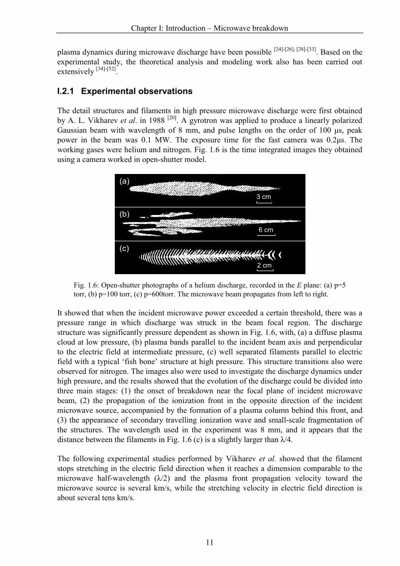
The detail structures and filaments in high pressure microwave discharge were first obtained by A. L. Vikharev et al. in 1988 [20]. A gyrotron was applied to produce a linearly polarized Gaussian beam with wavelength of 8 mm, and pulse lengths on the order of 100 µs, peak power in the beam was 0.1 MW. The exposure time for the fast camera was 0.2µs. The working gases were helium and nitrogen. Fig. 1.6 is the time integrated images they obtained using a camera worked in open-shutter model.
Fig. 1.6: Open-shutter photographs of a helium discharge, recorded in the E plane: (a) p=5 torr, (b) p=100 torr, (c) p=600torr. The microwave beam propagates from left to right.
It showed that when the incident microwave power exceeded a certain threshold, there was a pressure range in which discharge was struck in the beam focal region. The discharge structure was significantly pressure dependent as shown in Fig. 1.6, with, (a) a diffuse plasma cloud at low pressure, (b) plasma bands parallel to the incident beam axis and perpendicular to the electric field at intermediate pressure, (c) well separated filaments parallel to electric field with a typical ‘fish bone’ structure at high pressure. This structure transitions also were observed for nitrogen. The images also were used to investigate the discharge dynamics under high pressure, and the results showed that the evolution of the discharge could be divided into three main stages: (1) the onset of breakdown near the focal plane of incident microwave beam, (2) the propagation of the ionization front in the opposite direction of the incident microwave source, accompanied by the formation of a plasma column behind this front, and (3) the appearance of secondary travelling ionization wave and small-scale fragmentation of the structures. The wavelength used in the experiment was 8 mm, and it appears that the distance between the filaments in Fig. 1.6 (c) is a slightly larger than λ/4.
The following experimental studies performed by Vikharev et al. showed that the filament stops stretching in the electric field direction when it reaches a dimension comparable to the microwave half-wavelength (λ/2) and the plasma front propagation velocity toward the microwave source is several km/s, while the stretching velocity in electric field direction is about several tens km/s.
(a)
(b)
(c)
3 cm
6 cm
2 cm
Chapter I: Introduction – Microwave breakdown
12
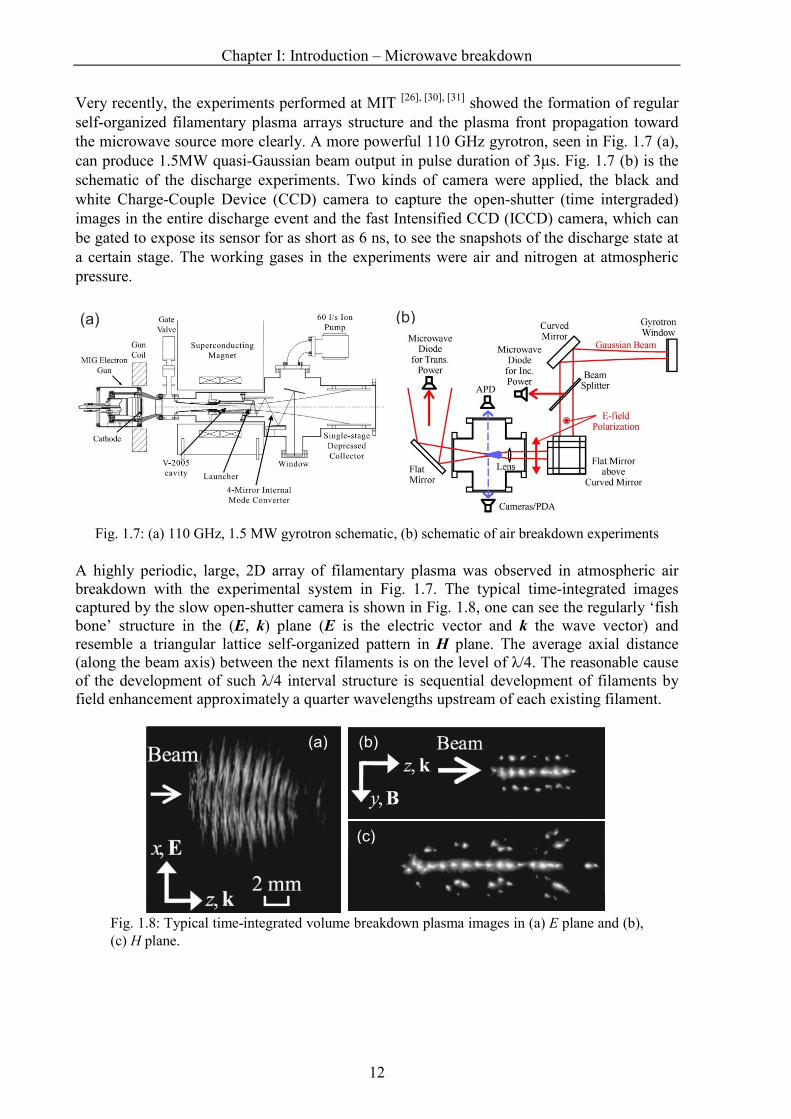
Very recently, the experiments performed at MIT [26], [30], [31] showed the formation of regular self-organized filamentary plasma arrays structure and the plasma front propagation toward the microwave source more clearly. A more powerful 110 GHz gyrotron, seen in Fig. 1.7 (a), can produce 1.5MW quasi-Gaussian beam output in pulse duration of 3µs. Fig. 1.7 (b) is the schematic of the discharge experiments. Two kinds of camera were applied, the black and white Charge-Couple Device (CCD) camera to capture the open-shutter (time intergraded) images in the entire discharge event and the fast Intensified CCD (ICCD) camera, which can be gated to expose its sensor for as short as 6 ns, to see the snapshots of the discharge state at a certain stage. The working gases in the experiments were air and nitrogen at atmospheric pressure.
Fig. 1.7: (a) 110 GHz, 1.5 MW gyrotron schematic, (b) schematic of air breakdown experiments
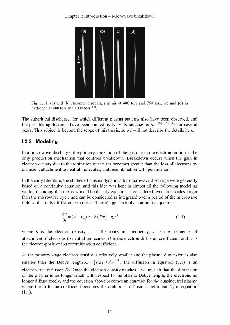
A highly periodic, large, 2D array of filamentary plasma was observed in atmospheric air breakdown with the experimental system in Fig. 1.7. The typical time-integrated images captured by the slow open-shutter camera is shown in Fig. 1.8, one can see the regularly ‘fish bone’ structure in the (E, k) plane (E is the electric vector and k the wave vector) and resemble a triangular lattice self-organized pattern in H plane. The average axial distance (along the beam axis) between the next filaments is on the level of λ/4. The reasonable cause of the development of such λ/4 interval structure is sequential development of filaments by field enhancement approximately a quarter wavelengths upstream of each existing filament.
Fig. 1.8: Typical time-integrated volume breakdown plasma images in (a) E plane and (b), (c) H plane.
(a) (b)
(a) (b)
(c)
Chapter I: Introduction – Microwave breakdown
13
Fig. 1.9: Images of breakdown in ambient of air at 710 torr in H plane with 49 ns optical gate pulse starting at (a) t=400 ns, (b) 1.28µs, and (c) 1.52µs.
Plasma images taken in the (H, k) plane (H is the magnetic vecotor) are shown in Fig. 1.9 in ambient of air at a pressure of 710 torr. The black and white images of Fig. 1.9 were time-integrated as in Fig. 1.8, and the pseudo colour images were taken by the fast gated camera with 49 ns optical gate width. One can check that the plasma/ionization front propagation velocity toward the microwave source is more than a dozen km/s, which agrees with Vikharev’s observation.
In order to investigate the streamer stretching in the (E, k) plane, an open cavity formed by two coaxial spherical concave mirrors as shown in Fig. 1.10 [53] was applied in experiments. With a certain distance between the mirrors, a linearly polarized standing TEM wave along the cavity axis can be obtained. So with this experimental arrangement a single streamer could be isolated at the antinode of the standing wave field resulting from the incident and reflected microwaves. The experiments were performed in different gases and different pressure with a 3.2 GHz incident microwave.
Fig. 1.10: Experimental arrangement for investigating microwave streamer discharges in an open two mirror cavity: (1) gyrotron, (2) circulator, (3) matching transmission line, (4) open cavity with spherical mirrors, (5) gas filled cell, and (6) connection to an oscillograph.
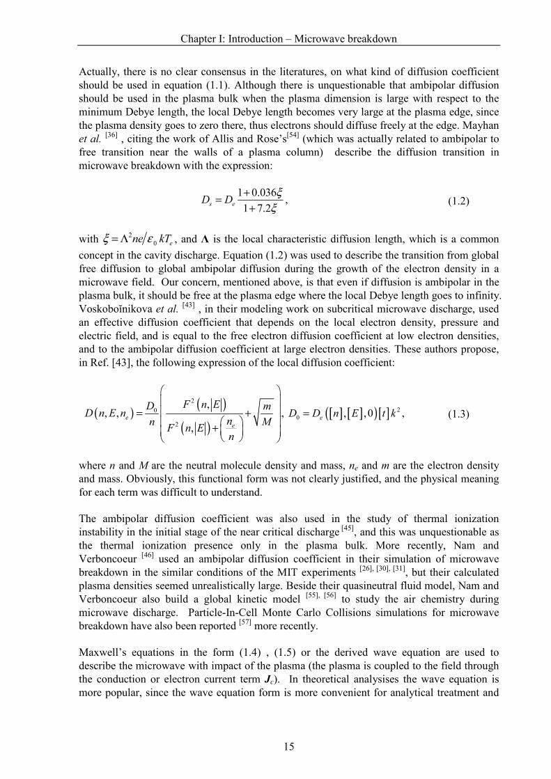
Regardless of the shape detail of the streamer, the visible streamer length in Fig. 1.11 was about 2.5 cm for different work gases, and was found to depend weakly on pressure. This length is on the level of quarter wavelength (λ/4), which is quite smaller than λ/2 obtained by Vikharev and the filament length in Fig. 1.8 (a).
(a)
(b)
(c)
Chapter I: Introduction – Microwave breakdown
14
Fig. 1.11: (a) and (b) streamer discharges in air at 480 torr and 760 torr, (c) and (d) in hydrogen at 480 torr and 1000 torr [53].
The subcritical discharge, for which different plasma patterns also have been observed, and the possible applications have been studied by K. V. Khodataev el al. [15], [19], [43] for several years. This subject is beyond the scope of this thesis, so we will not describe the details here.
I.2.2 Modeling
In a microwave discharge, the primary ionization of the gas due to the electron motion is the only production mechanism that controls breakdown. Breakdown occurs when the gain in electron density due to the ionization of the gas becomes greater than the loss of electrons by diffusion, attachment to neutral molecules, and recombination with positive ions.
In the early literature, the studies of plasma dynamics for microwave discharge were generally based on a continuity equation, and this idea was kept in almost all the following modeling works, including this thesis work. The density equation is considered over time scales larger than the microwave cycle and can be considered as integrated over a period of the microwave field so that only diffusion term (no drift term) appears in the continuity equation:
( ) ( ) 2i a ei
nn Dn r n
tν ν
∂= − + ∆ −
∂. (1.1)
where n is the electron density, iν is the ionization frequency, aν is the frequency of
attachment of electrons to neutral molecules, D is the electron diffusion coefficient, and rei is the electron-positive ion recombination coefficient.
At the primary stage electron density is relatively smaller and the plasma dimension is also
smaller than the Debye length ( )1 22
0D ekT e nλ ε= , the diffusion in equation (1.1) is an
electron free diffusion De. Once the electron density reaches a value such that the dimension of the plasma is no longer small with respect to the plasma Debye length, the electrons no longer diffuse freely, and the equation above becomes an equation for the quasineutral plasma where the diffusion coefficient becomes the ambipolar diffusion coefficient Da in equation (1.1).
(a) (b) (c) (d)
1 cm
Chapter I: Introduction – Microwave breakdown
15
Actually, there is no clear consensus in the literatures, on what kind of diffusion coefficient should be used in equation (1.1). Although there is unquestionable that ambipolar diffusion should be used in the plasma bulk when the plasma dimension is large with respect to the minimum Debye length, the local Debye length becomes very large at the plasma edge, since the plasma density goes to zero there, thus electrons should diffuse freely at the edge. Mayhan et al. [36] , citing the work of Allis and Rose’s[54] (which was actually related to ambipolar to free transition near the walls of a plasma column) describe the diffusion transition in microwave breakdown with the expression:
1 0.036
1 7.2s eD D
ξ
ξ
+=
+, (1.2)
with 20 ene kTξ ε= Λ , and Λ is the local characteristic diffusion length, which is a common
concept in the cavity discharge. Equation (1.2) was used to describe the transition from global free diffusion to global ambipolar diffusion during the growth of the electron density in a microwave field. Our concern, mentioned above, is that even if diffusion is ambipolar in the plasma bulk, it should be free at the plasma edge where the local Debye length goes to infinity. Voskoboĭnikova et al. [43] , in their modeling work on subcritical microwave discharge, used an effective diffusion coefficient that depends on the local electron density, pressure and electric field, and is equal to the free electron diffusion coefficient at low electron densities, and to the ambipolar diffusion coefficient at large electron densities. These authors propose, in Ref. [43], the following expression of the local diffusion coefficient:
( )( )
( )
2
0
2
,, ,
,e
e
F n ED mD n E n
nn MF n E
n
= +
+
, [ ] [ ]( )[ ] 20 , , 0
eD D n E t k= , (1.3)
where n and M are the neutral molecule density and mass, ne and m are the electron density and mass. Obviously, this functional form was not clearly justified, and the physical meaning for each term was difficult to understand.
The ambipolar diffusion coefficient was also used in the study of thermal ionization instability in the initial stage of the near critical discharge [45], and this was unquestionable as the thermal ionization presence only in the plasma bulk. More recently, Nam and Verboncoeur [46] used an ambipolar diffusion coefficient in their simulation of microwave breakdown in the similar conditions of the MIT experiments [26], [30], [31], but their calculated plasma densities seemed unrealistically large. Beside their quasineutral fluid model, Nam and Verboncoeur also build a global kinetic model [55], [56] to study the air chemistry during microwave discharge. Particle-In-Cell Monte Carlo Collisions simulations for microwave breakdown have also been reported [57] more recently.
Maxwell’s equations in the form (1.4) , (1.5) or the derived wave equation are used to describe the microwave with impact of the plasma (the plasma is coupled to the field through the conduction or electron current term Jc). In theoretical analysises the wave equation is more popular, since the wave equation form is more convenient for analytical treatment and
Chapter I: Introduction – Microwave breakdown
16
can be solved in the same time step with the plasma model. But with Maxwell’s equations (1.4) and (1.5) the interaction between microwave and plasma can be seen more clearly.
c
EH J
tε
∂∇ × = +
∂ (1.4)
HE
tµ
∂∇× = −
∂ (1.5)
As said above, the plasma model is coupled to Maxwell’s equations through the conduction current in equation (1.6). As the ion current is much smaller with respecting to the electron current, the conduction current in Maxwell’s equations is mostly the electron current.
c en= −J u (1.6)
where the electron mean velocity u is obtained from the simplified electron momentum transfer equation given by
m
e
t mν
∂= − −
∂
uE u , (1.7)
with mν the momentum transfer collision frequency between electrons and neutral molecules.
We will see in the next chapter that with the local field approximation the ionization
frequency in the density equation is a function of a reduced effective field ( effE p ).
Empirical analytical expressions (from experimental data) of the ionization frequency as a function of reduced effective field are generally used in the literatures. These expressions are typically of the forms (1.8) and (1.9) [7], [38], [41]:
, B p Eid d ev Ae v E
p
νµ−= = (1.8)
( ) ( )3 1 1
1 ,
4.9 10 , 32
i a
c
a c
E
p p E
Es torr V cm torr
p p
βν ν
ν − −
= −
× ⋅� �
(1.9)
I.3 The work of this thesis
The detailed understanding of the mechanisms leading to the plasma dynamics and formation of complex filamentary structures after microwave breakdown at high pressure is very important to evaluate the potential applications of microwave plasmas.
In this thesis work we try to establish a numerical model for the microwave breakdown discharge at high (atmospheric) pressure with clear physical concepts. The model is described
Chapter I: Introduction – Microwave breakdown
17
in Chapter II. In chapter II we first build a simple quasineutral fluid (diffusion-ionization-attachment-recombination) model for the plasma. The diffusion in this model is an effective diffusion with a parameter that describes the transition from free diffusion at the plasma edge to ambipolar diffusion inside the plasma bulk. The ionization and attachment frequencies are supposed to depend on the reduced effective field and the plasma density variations are averaged over one cycle of the microwave. The microwave is described with Maxwell’s equations. The numerical scheme for plasma equation and the finite-difference-time-domain (FDTD) scheme for Maxwell’s equations are also presented in this chapter, as well as the absorbing boundary condition (or outgoing boundary condition) proposed by Mur.
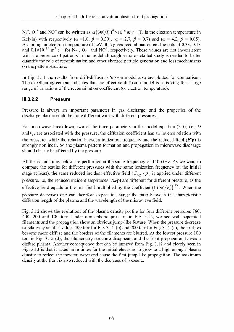
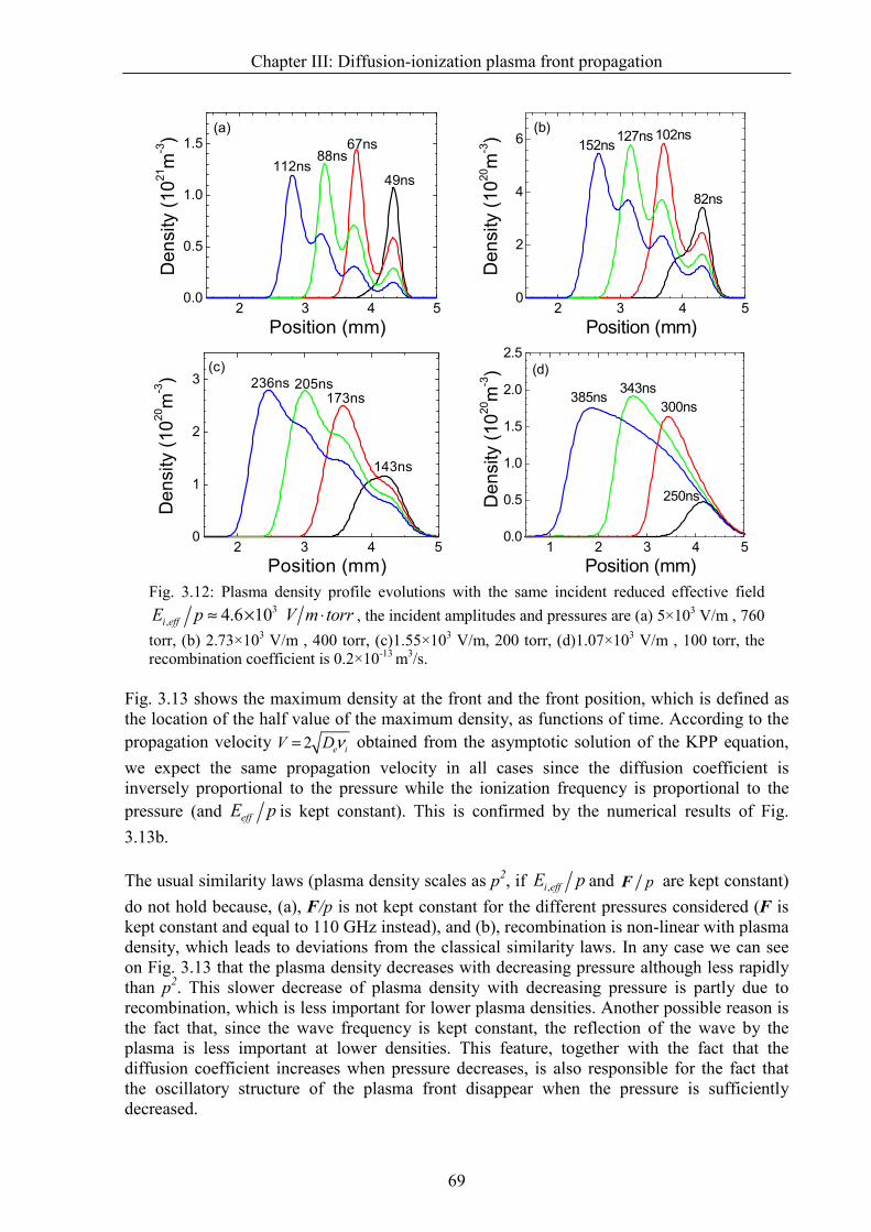
In Chapter III, the numerical validation of the effective diffusion coefficient for the collisional plasma that we propose for the density equation is performed in 1D by comparing the numerical results with the “more exact” solutions from a drift-diffusion-Poisson model. The comparisons are performed both for the simple cases of constant ionization frequencies and also for the realistic case when the plasma front propagates toward the microwave source in microwave breakdown. In the latter case the plasma model is solved together with Maxwell’s equations and the ionization frequency is modulated in time due to the complex interaction between the discharge plasma and the incident microwave. The mechanism of the plasma front propagating toward the incident microwave source is studied with 1D numerical result as well as the propagation velocity and distance between the filaments. The effects of electron-ion recombination, pressure, and negative ions are discussed also.
After the numerical validation of the effective diffusion coefficient and the 1D study on the plasma pattern formation and propagation in chapter III, the Maxwell’s equations are solved together with the quasineutral plasma model equations in 2D to study the space and time evolution of the microwave field and the plasma density in chapter IV. The simulations in both (H, k) and (E, k) plan are performed, and the results provide a physical interpretation of the pattern formation and dynamics in terms of diffusion-ionization and absorption-reflection mechanisms. The simulations allow a good qualitative and quantitative understanding of different features of the microwave discharge plasma such as plasma front propagating velocity, spacing between filaments, and maximum density inside the filaments. The influence of the discharge parameters, i.e., recombination coefficient, pressure, and incident microwave power, on the development of the well defined filamentary plasma arrays or more diffuse plasma fronts also are studied parametrically.
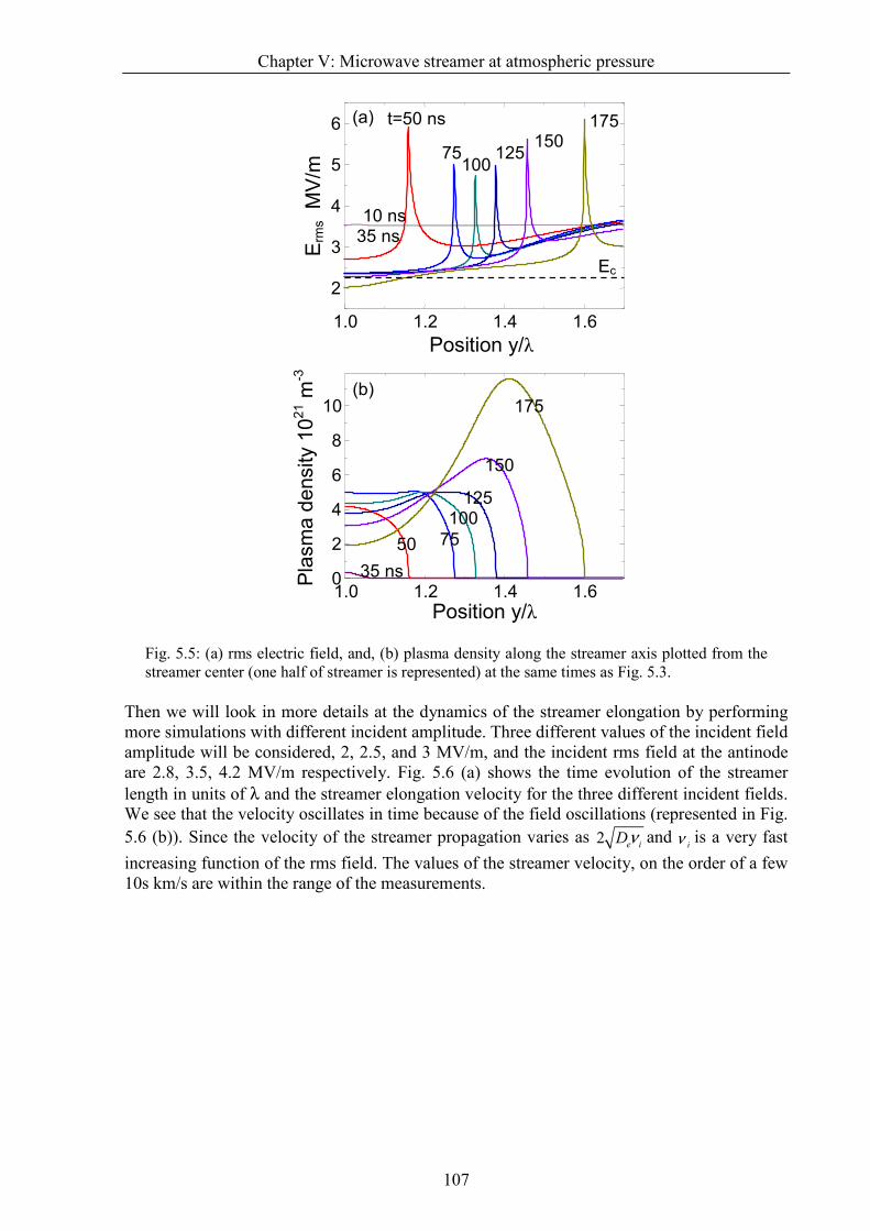
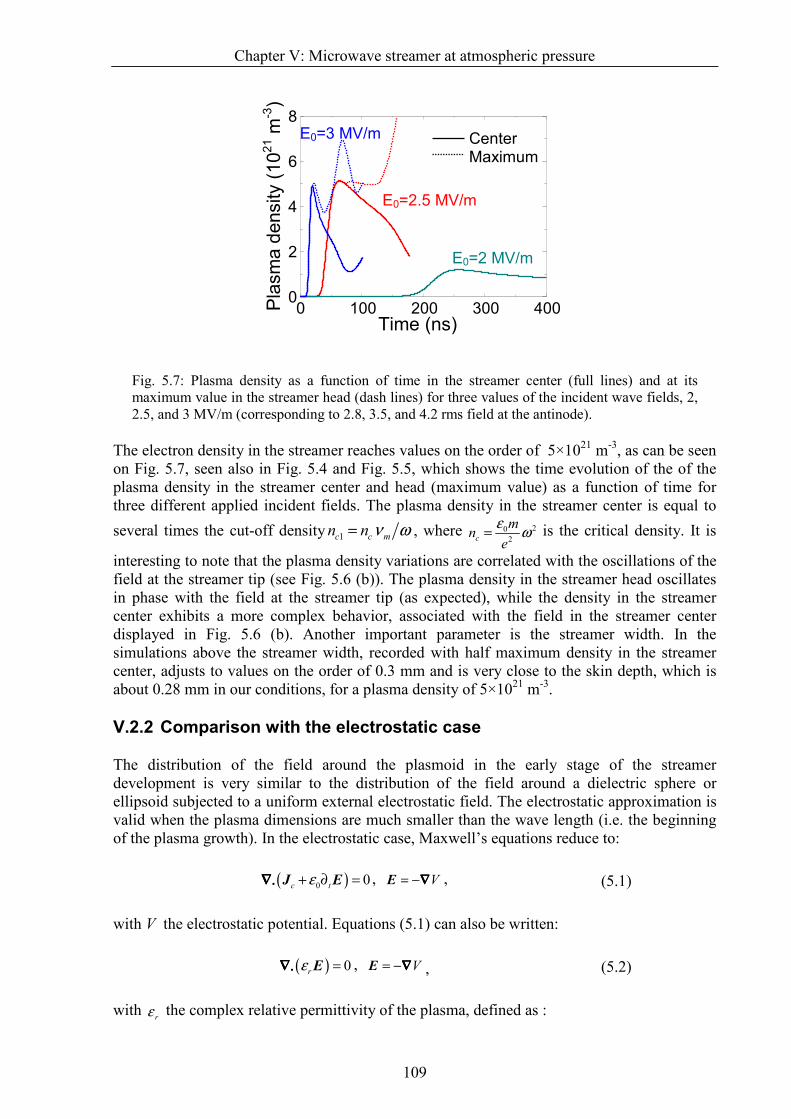
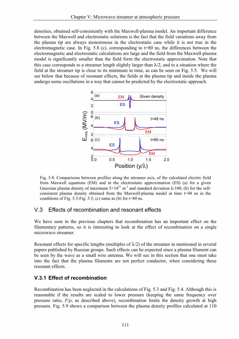
In Chapter V, the physics and the dynamics of a single microwave streamer formation and elongation in a standing microwave field are investigated. The standing wave is generated by two incident, identical, linearly polarized plane waves injected from the left and right sides of the simulation domain in a 2D rectangular geometry. The microwave streamer is initiated by assuming an initial density of seed electrons at the location of maximum electric field, i.e., antinode. The simulation provides the space and time evolution of the plasma density and electromagnetic field during the formation and elongation of the streamer under typical conditions. The properties of the streamer such as diameter, elongation velocity and maximum electric field at the streamer tip are discussed. Resonant effects leading to the existence of maxima and minima of the electric field at the streamer tips during the streamer elongation are also discussed.
Chapter I: Introduction – Microwave breakdown
18
Even though all the simulations in this thesis are performed with the frequency of 110 GHz in ambient of dry air at atmospheric pressure, the model results can be extrapolated (at least in an approximate way) to lower frequencies if one remembers that in the absence of second kind collisions (such as electron-ion recombination) similar discharge are obtained when the following parameters are kept constant: F/p, E/p, pt, pr, n/p2 (F is the macroscopic force, p is the pressure, t the time, r the position in space). Finally we note that in all the results presented in this thesis, the gas temperature and gas density are supposed to be constant. In the conditions of microwave breakdown at atmospheric pressure the plasma electrons can absorb a significant amount of energy from the microwave field. A non negligible part of this energy can be quickly transferred into gas heating, leading to an increase of the gas temperature, followed by a decrease of the gas density (associated in some cases with the formation of a shockwave). Such effect may become important when time scale becomes on the order of 100 ns but is not considered in the work presented in this thesis.
I.4 Conclusion
Microwave discharge has been studied for more than a half century. After the gyrotrons became available for lab researches, the discharge in open space with a microwave under high pressure was investigated experimentally. Thanks to the development of high-speed imaging techniques, the self-organized small-scale plasma structures in high pressure microwave discharge and the dynamics have been observed in details. The detailed dynamics of the self-organized structures and microwave streamer formation, which are still not very clear, can be fully understood with the help of an accurate enouth numerical modeling. In this thesis a quasineutral plasma model with an effective diffusion is established for microwave discharge and solved together with the Maxwell’s equations. The thesis work shows that most of the observed complex features and plasma dynamics of microwave discharge at atmospheric pressure can be described and understood with the help of this simple Maxwell-quasineutral model.
Chapter I: Introduction – Microwave breakdown
19
References
[1] A. D. MacDonald, Microwave Breakdown in Gases (John Wiley & Sons, New York, 1966).
[2] F. Paschen. Ueber die zum Funkenübergang in Luff, Wasserstoff und Kohlensäure bei verschiedenen Drucken erforderliche Potentialdifferenz. Wied. Ann., 37:69-96, 1889.
[3] J. S. Townsend. The Theory of Ionization of Gases by Collision. Constable & Company Ltd., London, 1910.
[4] I. Langmuir. The Interaction of Electron and Positive Ion Space Charges in Cathode Sheaths. Phys. Rev. 33, 954–989 (1929)
[5] L. Tonks and I. Langmuir. A General Theory of the Plasma of an Arc. Phys. Rev. 34, 876–922 (1929)
[6] H. M. Mott-Smith and I. Langmuir. The Theory of Collectors in Gaseous Discharges. Phys. Rev. 28, 727–763 (1926)
[7] Yu. P. Raizer. Gas Discharge Physics. (Springer, Berlin, 1991).
[8] W. Bartholomeyczyk. Über den Mechanismus der Zündung langer Entladungsrohre. Ann. der Physik, 5:485–520, 1939.
[9] O. Svelto, Principles of lasers, fifth edition, Springer Science and Business Media,Inc., 2009.
[10] V. L. Bratman et al. Plasma creation by terahertz electromagnetic radiation. Physics of Plasmas. 18, 083507 (2011)
[11] Annemie Bogaerts, Erik Neyts, Renaat Gijbels, Joost van der Mullen. Gas discharge plasmas and their applications. Spectrochimica Acta Part B 57 (2002) 609–658
[12] Yoshiyuki Takao, et al. Performance test of micro ion thruster using microwave discharge. Vacuum Volume 80, Issues 11-12, 7 September 2006, Pages 1239-1243
[13] K. D. Diamant, B. L. Zeigler, and R. B. Cohen. Microwave Electrothermal Thruster Performance. Journal of Propulsion and Power. Vol. 23, No. 1, Jan.–Feb. 2007
[14] X. W. Han, G. W. Mao and H. Q. He. The PIC-DSMC Numerical Simulation for Vacuum Plume of MPT. Journal of Solid Rocket Technology, vol.25 (2002), pp21-24
[15] Kirill V. Khodataev. Microwave Discharges and Possible Applications in Aerospace Technologies. Journal of Propulsion and Power. Vol.24, No.5, 2008
[16] Yasuhisa Oda and Kimiya Komurasaki, Koji Takahashi, Atsushi Kasugai, and Keishi Sakamoto. Plasma generation using high-power millimeter-wave beam and its application for thrust generation. Journal of Applied Physics 100, 113307 (2006)
[17] V. L. Bychkov, I. I.Esakov, L. P.Grachev, K. V.Khodataev. A Microwave Discharge Initiated by Loop-Shaped Electromagnetic Vibrator on a Surface of Radio-Transparent Plate in Airflow. 46th AIAA Aerospace Sciences Meeting and Exhibition, 7-10 January 2008, Reno, Nevada
[18] K. V.Khodataev. Numerical study of the contactlessly fed vibrators system destined for at surface airflow heating. 47th AIAA Aerospace Sciences Meeting and Exposition, 5 - 8 January 2009, Orlando, Florida
Chapter I: Introduction – Microwave breakdown
20
[19] I. I.Esakov, L. P.Grachev, K. V.Khodataev, and D.M.Van Wie. Deeply subcritical MW discharge in the submerged stream of propane-air mixture. 46th AIAA Aerospace Sciences Meeting and Exhibition, 7-10 January 2008, Reno, Nevada
[20] A. L. Vikharev, et al. Nonlinear dynamics of a freely localized microwave discharge in an electromagnetic wave beam. Sov. Phys. JETP 67 724 (1988)
[21] W. M. Bollen, C. L. Yee, A. W. Ali, M. J. Nagurney, and M. E. Read. High-power microwave energy coupling to nitrogen during breakdown. J. Appl. Phys. 54, 101 (1983)
[22] S. P. Kuo and Y. S. Zhang, P. Kossey. Propagation of high power microwave pulses in air breakdown environment. J. Appl. Phys. 67 (6), 15 March 1990
[23] M. Lǒfgren, D. Anderson, H. Bonder, H. Hamnén, and M. Lisak. Breakdown phenomena in microwave transmit-receive switches. J. Appl. Phys. 69 (4), 15 February 1991
[24] A. L. Vikharev, A. M. Gorbachev, A. V. Kim, and A. L. Kolsyko. Formation of the small-scale structure in a microwave discharge in high-pressure gas. Sov. J. Plasma Phys. 18 554 (1992)
[25] I. I. Esakov, L. P. Grachev, K. V. Khodataev and D.M.Van Wie. Microwave Discharge in Quasi-optical Wave Beam. 45th AIAA Aerospace Sciences Meeting and Exhibit, 8 - 11 January 2007, Reno, Nevada
[26] A. Cook, M. Shapiro, and R. Temkin. Pressure dependence of plasma structure in microwave gas breakdown at 110 GHz. App. Phys. Lett. 97, 011504 (2010)
[27] A. Litvak. Freely localized gas discharges in microwave beams. Applications of high power microwaves, edited by A.V. Gaponov-grekhov and V.L. Granatstein(Artech House, Boston, 1994), pp. 145-167
[28] S. Popović R. J. Exton and G. C. Herring. Transition from diffuse to filamentary domain in a 9.5 GHz microwave-induced surface discharge. App. Phys. Lett. 87, 061502 2005
[29] I. I. Esakov, L. P. Grachev, K. V. Khodataev, V. L. Bychkov, and D. M. Van Wie. Surface Discharge in a Microwave Beam. IEEE Trans. On Plasma Sci., Vol.35, No.6, Dec. 2007
[30] Y. Hidaka, E.M. Choi, I. Mastovsky, M.A. Shapiro, J.R. Sirigiri, and R. J. Temkin. Observation of Large Arrays of Plasma Filaments in Air Breakdown by 1.5-MW 110-GHZ Gyrotron Pulses. Phys. Rev. Lett. 100, 035003 (2008)
[31] Y. Hidaka, E. M. Choi, I. Mastovsky, M. A. Shapiro, J. R. Sirigiri, R. J. Temkin, G. F. Edmiston, A. A. Neuber, Y. Oda. Plasma structures observed in gas breakdown using a 1.5 MW, 110 GHz pulsed gyrotron. Phys. of plasma 16, 055702 (2009)
[32] R. P. Cardoso, T. Belmonte, C. Noël, F. Kosior, and G. Henrion. Filamentation in argon microwave plasma at atmospheric pressure. J. Appl. Phys 105, 093306 2009
[33] A. M. Cook, J. S. Hummelt, M. A. Shapiro, and R. J. Temkin. Measurements of electron avalanche formation time in W-band microwave air breakdown. Phys. Plasmas 18, 080707 (2011)
[34] L. Gould and L. W. Roberts. Breakdown of Air at Microwave Frequencies. J. Appl. Phys, Vol.27, No.10, Oct. 1956
Chapter I: Introduction – Microwave breakdown
21
[35] J. T. Mayhan and R. L. Fante. Microwave Breakdown Over a Semi-Infinite Interval. J. Appl. Phys, Vol 40, No. 13, Dec. 1969
[36] J. T. Mayhan. Compression of Various Microwave Breakdown Prediction Models. J. Appl. Phys, Vol.42, No.13, Dec. 1971
[37] W. Woo and J. S. DeGroot. Microwave absorption and Plasma heating due to microwave breakdown in the atmosphere. Phys. Fluids, Vol.27, No.2, Feb. 1984
[38] D. Anderson, M. Lisak, and T. Lewin. Self-consistent structure of an ionization wave produced by microwave breakdown in atmospheric air. Phys. Fluids 29(2), Feb. 1986
[39] S. P. Kuo and Y. S. Zhang, Paul Kossey. Propagation of high power microwave pulses in air breakdown environment. J. Appl. Phys. 67 (6), 15 March 1990
[40] S. P. Kuo and Y. S. Zhang. A theoretical model for intense microwave pulse propagation in an air breakdown environment. Phys. Fluids B 3, 2906 (1991),
[41] H. Hamnén, D. Anderson, and M. Lisak. A model for steady-state breakdown plasmas in microwave transmit-receive tubes. J. Appl. Phys. 70 (1), 1 July I991
[42] M. Löfgren, D. Anderson, M. Lisak, and L. Lundgren. Breakdown-induced distortion of high-power microwave pulses in air. Phys. Fluids B, Vol. 3, No. 12, December 1991
[43] O. I. Voskoboĭnikova, S. L. Ginzburg, V. F. D’yachenko, and K. V. Khodataev. Numerical Investigation of Subcritical Microwave Discharges in a High-Pressure Gas. Tech. Phys. 2002,Vol. 47, No. 8, pp. 955–960
[44] A.F. Aleksandrov, V.L. Bychkov, L.P. Grachev, I.I. Esakov, and A. Yu. Lomteva. Air Ionization in a Near-Critical Electric Field. Tech. Phys. 2006, Vol. 51, No.3, pp.330-335
[45] V. L. Bychkov, L. P. Grachev, and I. I. Isakov. Thermal Ionization Instability of an Air Discharge Plasma in a Microwave Field. Tech. Phys. 2007, Vol. 52, No. 3, pp. 289–295
[46] Sang Ki Nam and John P. Verboncoeur. Theory of Filamentary Plasma Array Formation in Microwave Breakdown at Near-Atmospheric Pressure. Phys. Rev. Lett. 103, 055004 (2009)
[47] J. P. Boeuf, B. Chaudhury, and G. Q. Zhu. Theory and Modeling of Self-Organization and Propagation of Filamentary Plasma Arrays in Microwave Breakdown at Atmospheric Pressure. Phys. Rev. Lett. 104, 015002 ( 2010)
[48] B. Chaudhury and J. P. Boeuf. Computational Studies of Filamentary Pattern Formation in a High Power Microwave Breakdown Generated Air Plasma. IEEE Trans. on plasma Sci., VOL. 38, NO. 9, SEPTEMBER 2010
[49] B. Chaudhury, J. P. Boeuf, and G. Q. Zhu. Pattern formation and propagation during microwave breakdown. Phys. of plasma 17, 123505 (2010)
[50] G. Q. Zhu, J. P. Boeuf, and B. Chaudhury. Ionization-diffusion plasma front propagation in a microwave field. Plasma Sources Sci. Technol. 20 (2011)035007
[51] B. Chaudhury, J. P. Boeuf, and G. Q. Zhu. Physics and modeling of Microwave Streamers at atmospheric pressure. J. Appl. Phys., submitted.
[52] Qianhong Zhou and Zhiwei Dong. Modeling study on pressure dependence of plasma structure and formation in 110 GHz microwave air breakdown. App. Phys. Lett. 98,
Chapter I: Introduction – Microwave breakdown
22
161504 (2011)
[53] V. S. Barashenkov, L. P. Grachev, I. I. Esakov, B. F. Kostenko, K. V. Khodataev, and M. Z. Yur’ev. Threshold for a cumulative resonant microwave streamer discharge in a high-pressure gas. Tech. Phys. 2000, Vol. 45, No. 11, pp. 1406–1410
[54] W. P. Allis, D. J. Rose. The Transition from Free to Ambipolar Diffusion. Phys. Rev. Vol. 93, No. 1, 84-93 (1954)
[55] Sang Ki Nam and J. P. Verboncoeur. Effect of microwave frequency on breakdown and electron energy distribution function using a global model. App. Phys. Lett. 93, 151504 2008
[56] Sang Ki Nama, J. P. Verboncoeur. Global model for high power microwave breakdown at high pressure in air. Computer Physics Communications 180 (2009) 628–635
[57] J. T. Krile, A. A. Neuber, H. G. Krompholz, and T. L. Gibson. Monte Carlo simulation of high power microwave window breakdown at atmospheric conditions. App. Phys. Lett. 89, 201501 2006
[58] V. A. Bityurin and P. V. Vedenin. Electrodynamic Model of a Microwave Streamer. Technical Physics Letters, 2009, Vol. 35, No. 7, pp. 622–625
[59] V. A. Bityurin and P. V. Vedenin, "Dynamics of Power Absorption in a Microwave Streamer", Technical Physics Letters, 2009, Vol. 35, No. 8, pp. 683–686
[60] V. A. Bityurin and P. V. Vedenin. An Integral Approach to Considering the Evolution of a Microwave Streamer. J. Exp. and Theo. Phys., 2010, Vol. 111, No. 3, pp. 512–521
[61] W. J. M. Brok. Modelling of transient phenomena in gas discharges. PhD. thesis, Technische Universiteit Eindhoven, The Netherlands, 2005
Chapter II: Models of microwave breakdown
23
Chapter II
Modeling of microwave breakdown
Chapter II: Models of microwave breakdown
24
Chapter II: Models of microwave breakdown
25
II.1 Introduction
Experimental physics provides essential ingredients to the understanding of natural phenomena, but sometimes the experiment is limited as the interest quantity cannot be observed directly and needs to be inferred via an interpretation that introduces assumptions. Numerical modeling provides a way to complement experiments by numerical solutions to the complete set of equations that is believed to describe the system. Different from experimental observations, all quantities can be obtained and how they influence each other also can be tested by artificially manipulating them. The observable quantities can be directly compared to the experimental data and this can increase the confidence in the validity of the model. Finally, model results can inspire new experiments, help interpret observations or validate a given interpretation of experiments by performing a “numerical experiment”.
The complete set of equations that is necessary to describe a given system, i.e. the physical model of the considered system, is the foundation of the numerical experiment, and the theory analysis on the set of equations also plays a guiding role in the simulation works. In this chapter we will try to establish a closed physical model for the discharge plasma in microwave breakdown at atmospheric pressure. In the model, an effective diffusion coefficient, different from reported ones, will be introduced to describe the diffusion transition from free diffusion at the plasma front to ambipolar in the plasma bulk. After the model description, the principles of the numerical method will be introduced. The coupling between the microwave fields and the discharge plasma will be discussed in detail in a separated section.
II.2 Physics
II.2.1 Microwave and Maxwell’s equations
The existence of electromagnetic wave was first predicted by J. C. Maxwell in 1861 [1] and confirmed by H. Hertz subsequently. After it was first used in the wireless telegraphy by G. Marconi in 1895, the applications of electromagnetic wave developed explosively. Nowadays these applications can be seen everywhere around us, for example in mobile phones, wireless LAN protocols, satellite communications and navigations.
Electromagnetic waves can be classified according to the wavelengths (or frequencies). On the electromagnetic spectrum Fig. 2.1, one can see that the band of microwave is between the radio frequency and the infrared, with wavelengths ranging from as long as 1 m to as short as 1 mm (or with frequencies from 200 MHz to 200GHz). Of course the boundaries for the adjacent bands are not strictly defined.
Fig. 2.1: Electromagnetic spectrum
Chapter II: Models of microwave breakdown
26
Maxwell’s equations are a set of four equations, which firstly appeared throughout J. C. Maxwell’s 1861 paper [1]. Maxwell’s equations are the basis of macroscopic electromagnetic theory, which is the most basic and important theory for analyzing and studying electromagnetic problems. Maxwell’s equations can be written in many different forms. Here we present the basic differential time domain form in a linear isotropic medium:
c
EH J
tε
∂∇ × = +
∂ (2.1)
HE
tµ
∂∇× = −
∂ (2.2)
( )Eε ρ∇ =i (2.3)
( ) 0Hµ∇ =i (2.4)
where, 0rε ε ε= , 0rµ µ µ= , 0ε and 0µ are permittivity and permeability of free space, rε and
rµ are relative values of permittivity and permeability for a specific linear isotropic medium
respectively, for free space and air the values of rε and rµ can be considered as one.
The first equation (2.1) is total current equations, it is Ampère’s circuital law with Maxwell’s bound current correction, the second (2.2) is Maxwell-Faraday equation derived from Faraday’s law of induction, (2.3) and (2.4) are Gauss’s law for electric field and magnetic field respectively. These four equations represent all the information needed for linear isotropic mediums to completely specify the electromagnetic behavior over time as long as the initial state is specified and satisfies the equations. Conveniently, the field and sources can be set to zero at the initial time. The two divergence equations (2.3) and (2.4) are in fact redundant as they are included within the curl equations and the initial conditions.
II.2.2 Fluid models for plasma
Models of a discharge should be build upon a microscopic description of the particles in the discharge, however the discharge gas in this work is air, which is a mixture with complex compositions (N2, O2, CO2, Ar, etc.). It will be a formidable (and unnecessary, considering our purpose) work to describe the behaviors of every particle species in the discharge. Therefore we simply treat the ionized air as a mixture of one type of positive ions, electrons and neutral particles, and pursue a ‘simple’ model to describe the evolution of the discharge plasma. The existence of different types of ions would only affect the ambipolar diffusion coefficient in our model and we will see below that the plasma dynamics is mainly affected by the free electron diffusion. Therefore we can consider that the presence of different types of ions is not an essential aspect of the physical mechanisms we want to describe.
The description of discharge plasma can be performed with fluid or particle models. And if some particle species of the plasma are described with fluid model while other species are described with particle model, the system is referred as “hybrid” model. Regardless the classification, all the plasma models are founded on the Boltzmann equation. This equation results from the notion of a grand canonical ensemble, the Liouville equation, in statistical
Chapter II: Models of microwave breakdown
27
mechanics, and the assumption that the particle ensemble under consideration is sufficiently large to ensure that statistical fluctuations are small enough to be neglected.
The Boltzmann equation describes the evolution of the velocity distribution function ( , , )f tr v
of a single particle species, which gives the particle number of specific species per unit phase volume with velocity v at the location r and at time t. The general form of the Boltzmann equation reads:
c
f ff f
t m t
∂ ∂ + ⋅∇ + ⋅∇ =
∂ ∂ v
Fv
, (2.5)
The left hands side reflects the flow of the particles in phase space, where m is the particle mass, F is the macroscopic forces (electro-magnetic and gravity forces) that cause the acceleration of the species, ∇v indicates the gradient operator in velocity space. The right
hands side of the equation ( )c
f t∂ ∂ denotes the effect of the microscopic collisions and
radiation. Coupling multiple Boltzmann equations for the different species together with their right hands side is necessary to describe a discharge. However, this seven-dimensional equation cannot be solved completely for any practical application at present, even for a single species.
In this thesis work we are interested in fluid description, which is applicable to low Knudsen number conditions, i.e., the mean free path of particles is significantly smaller than the characteristic dimension of the plasma. In fluid models the behaviors of various discharge particle species are described in terms of average, macroscopic, hydrodynamic quantities such as particle density n, mean velocity u, and mean energy ε. All those macroscopic quantities correspond to velocity moments of the distribution function ( , , )f tr v :
( ), ( , , )n t f t d= ∫r r v v (2.6)
1( , , )f t d
n= ∫u = v v r v v (2.7)
2 2 ( , , )2 2
m mv f t d
nε = = ∫v r v v . (2.8)
The fluid equations, describing the evolution of the macroscopic variables, can be obtained by taking different velocity moments of Boltzmann equation (2.5).
Multiplying Boltzmann equation by some function of velocity ( )Φ v and integrating over all
velocity components gives the transport equation for the average moment quantity given by
1( ) ( ) fd
nΦ = Φ∫v v v . (2.9)
The first term on the left hands side of Boltzmann’s equation becomes
Chapter II: Models of microwave breakdown
28
nf fd d
t t t
∂ Φ∂ ∂ ΦΦ = =
∂ ∂ ∂∫ ∫v v ,
where the order of integration and derivation have been changed.
Assuming the integration limits do not depend on r and t, the second term reads
( )fd nΦ ⋅∇ = ∇⋅ Φ∫ v v v ,
as Φ is independence of r.
For the macroscopic force term we have
( )1 n n
fd f dm m m m
Φ ⋅∇ = ∇ Φ − ⋅∇ Φ = − ⋅∇ Φ∫ ∫v v v v
Fv F v F F .
Here we have used the fact that f vanishes rapidly whenever → ∞v and hence the integration
over the full differential must vanish. As we also assumed that F is divergence free in velocity space, which holds true for the electromagnetic force. We denote the moment of the collision term as
c c
nfd
t t
∂ Φ ∂ Φ =
∂ ∂ ∫ v .
Combining these expressions we arrive at the general transport equation for the macroscopic
moment Φ ,
( )c
n nnn
t m t
∂ Φ ∂ Φ + ∇ ⋅ Φ − ⋅∇ Φ =
∂ ∂ vv F (2.10)
This equation has the form of conservation equation for the density of the average or
macroscopic quantity Φ . The right hands side describes the effect collisions. Now we are
free to choose the velocity functionΦ . As we can see, Φ=1 results in the particle continuity equation,
( )n
n St
∂+ ∇ ⋅ =
∂u , (2.11)
where the source term S is the net number of charged particles created per unit time per unit volume due to collisions.
Setting mΦ = v yields the momentum conservation equation,
Chapter II: Models of microwave breakdown
29
( )1n
n n Rt m m
∂+ ∇ ⋅ = − ∇ ⋅ + +
∂P
u Fuu (2.12)
where ( )( )m fd= − −∫P v u v u v is the pressure tensor, and mR n ν= u is the momentum source
due to momentum transfer collisions with other species, with mν the macroscopic momentum
transfer collision frequency.
And setting 22mΦ = v gives the energy conservation equation,
( )( )
nn n S
tε
εε
∂+ ∇ ⋅ + ⋅ + = ⋅
∂Pu u Q u F + (2.13)
where ( )2
2
mfd= − −∫Q v u v u v is the heat flux vector, Sε is the energy gained or lost in
collisions.
One crucial problem is that equations obtained from (2.20) are not closed, as the n-th moment equation introduces the (n+1)-th macroscopic moment, which is clear from the second term on the left hands side of the general transport equation (2.20). Any finite set of moment equations have more unknowns than equations. Therefore some additional information, limiting assumption or additional physical setting, is always needed to obtain a closed model. The first standard approximation for plasma is to assume that pressure tensor is diagonal and isotropic:
enT=P I (2.14)
where 2
3
menT fd= −∫ v u v is the scalar pressure, T is the temperature in unit of eV, and I is
the identity matrix. By substituting equations (2.11) and (2.14), the momentum conservation equation (2.12) becomes
( ) ( ) m
enT
t mn mν
∂+ ⋅∇ + ∇ = −
∂
u Fu u u . (2.15)
For high collisional conditions, i.e., discharges at high pressure, the charged particle momentum equation can be further simplified by removing the inertia term and the magnetic term included in the force term on the right hands, with respect to the collision term, assuming that collisions take place on much shorter time and smaller length scale than macroscopic field, pressure variations and cyclotron motion. With these assumptions the momentum conservation equation turns to be,
( ) ( )m m
q en n nT n Dn
m mµ
ν ν= = − ∇ ≡ ± −∇u E EΓΓΓΓ , (2.16)
with q the particle charge.
Chapter II: Models of microwave breakdown
30
This is the so-called drift-diffusion equation, and the two transport coefficients of mobility and diffusion:
mq mµ ν≡ (2.17)
mD eT mν≡ . (2.18)
These will be different for each particle species, and these two coefficients are connected by the Einstein relation:
D eT
qµ≡ . (2.19)
By these definitions the continuity equation can be rewritten in a drift-diffusion form
( )( )n
n Dn St
µ∂
+ ∇ ⋅ ± − ∇ =∂
E .
One of the main questions to close the fluid models is how to describe the source term in the equation, i.e., ionization, attachment and recombination. The most popular closure for collisional conditions is the local field approximation, assuming local equilibrium between electric acceleration, i.e., energy gain from the electric field, and collisional momentum and energy losses, so that the ionization frequencies depend only on the local electric field E, or rather, the reduced electric field E/N (or E/p) since the collision frequency is proportional to the gas density N (or pressure). Using the local field approximation the energy equation is not necessary anymore [2]. If we consider the ratio of diffusion coefficient and mobility to be constant, the diffusion coefficient in the equation above can be put out of nabla,
( )n
n D n St
µ∂
+ ∇ ⋅ ± − ∇ =∂
E . (2.20)
For charged particle in high frequency microwave field Maxwell’s and plasma equations are coupled with the conduction current density in the plasma, which generally reduces to the electron current density. The mean electron velocity for the electron current in high frequency fields is generally obtained from another approximation of the momentum equation (2.15). Assuming that the distance travelled over one field period is small with respect to the length scale of field and pressure variation, so all gradients can be neglected:
m
q
t mν
∂= −
∂
uE u . (2.21)
This simplified form of the electron momentum equation is appropriate in the calculation of the electron current in Maxwell’s equations on the time scale much shorter than the microwave period. On longer time scales, for example to describe electron transport averaged over one cycle, the diffusion term in the momentum transfer equations must be kept. Using two different forms of the momentum equations in the same model (equation (2.21) in the
Chapter II: Models of microwave breakdown
31
electron current in Maxwell’s equations and equation (2.15) in the plasma model) may appear inconsistent, but is justified as the different time scales are considered in the Maxwell’s equations and in the transport equations. Note also that equation (2.21) leads to the classical form of the complex permittivity (or complex conductivity) which is the basis of the Drude model and which defines the phase shift between microwave field and electron current density. Finally equation (2.21) is an expression for conditions without magnetic field. If an external magnetic field is present and its effect is not negligible the corresponding magnetic force must be added in the right hands side of equation (2.21). The magnetic field of the wave itself must also be included in some specific cases and leads to the so-called pondermotive effect. This effect is negligible in our conditions.
II.2.3 Quasineutral assumption and effective diffusion
In microwave discharge plasma, the electric field in equation (2.20) should be the sum of the microwave field and a DC or slowly varying space charge field. The wave field plays an essential role in electron heating and ionization, but its contribution to particle transport averaged over one wave cycle is negligible, so only space charge field contributes to charged particle transport, therefore equation (2.20) can be rewritten as,
( )sp
nn D n S
tµ
∂+ ∇ ⋅ ± − ∇ =
∂E (2.22)
where the space charge field is noted with Esp.
As mentioned before, we simply treat the ionized air in our problem as a mixture of positive ions, electrons and neutral particles. Two equations therefore are needed to describe the discharge plasma,
( )ee e sp e e
nn D n S
tµ
∂+ ∇ ⋅ − − ∇ =
∂E , (2.23)
( )ii i sp i i
nn D n S
tµ
∂+ ∇ ⋅ − ∇ =
∂E . (2.24)
In microwave field with the absence of DC field, quasineutrality ( e in n n= = ) is often a good
approximation. With the quasineutral approximation, we can write i e= =Γ Γ ΓΓ Γ ΓΓ Γ ΓΓ Γ Γ , and can
express the space charge (ambipolar) field as:
i esp
i e
D D n
nµ µ
− ∇=
+E . (2.25)
So the common flux is then given by
i e i e e ii i
i e i e
D D D Dn D n n
µ µµ
µ µ µ µ
− += ∇ − ∇ = − ∇
+ +ΓΓΓΓ .
Thus, equations (2.23) and (2.24) can be represented in a common form
Chapter II: Models of microwave breakdown
32
with a new diffusion coefficient
i e e ia
i e
D DD
µ µ
µ µ
+=
+, (2.27)
which is known as the ambipolar diffusion coefficient.
In most conditions, we can take e iµ µ� and Di is negligible with respect to De, so the
magnitude of Da can be estimated with
ia e
e
D Dµ
µ≈ . (2.28)
Equation (2.26) is a simple reaction-diffusion equation, which is also referred as the Fisher KPP (Kolmogorov-Petrovsky-Piskounov) equation [3] and arises in many other problems in chemistry, biology, geology and ecology. If neglecting the attachment and recombination in the source term, the well known asymptotic solution for equation (2.26) is a Gaussian of the form [4]:
( ) [ ]2 3, exp 4i an t At t D tν−= −r r . (2.29)
The density of this equation exhibits a self-similar front propagating at a speed of
2 i aV Dν= , (2.30)
and the characteristic length of the front, defined as 1
n n−
∇ in a reference frame moving at
the speed V, is
/a i
nL D
nν= =
∇. (2.31)
This result can be generalized [5] to more complex source terms, for example, including attachment and electron-ion recombination, i.e.,
( ) 2i a eiS n r nν ν= − − . (2.32)
The ambipolar diffusion coefficient above is obtained with the quasineutral assumption, which is valid in the bulk of a static plasma, but for the plasma in open space even if the plasma dimension is much larger than the Debye length, the plasma density at the edge goes to zero and, therefore, there should be a small region in the edge where the electrons diffuse
( )a
nD n S
t
∂− ∇ ⋅ ∇ =
∂, (2.26)
Chapter II: Models of microwave breakdown
33
freely instead of ambipolarly. This question has been considered somewhat empirically in the literature. Some authors [6] indicate that the calculated plasma propagation speed matches the experimental result only if the free diffusion coefficient is in equation (2.26). Theoretical evidence of the fact that the free diffusion coefficient should be used also has been provided which shows that within a DC electric field plasma streamer front propagates with a speed equal to the electron drift velocity at the front plus a corrective term due to diffusion and
equal to 2 i eDν [7], [8]. These results certainly can be applied to microwave discharge plasma,
where the cycle averaged electron drift velocity due to high-frequency electric field is zero [4],
and the speed of the front is therefore 2 i eDν , and the characteristic length of the propagation
front also turns to be /e iD ν .
Since free diffusion prevails only in the front while the plasma bulk is controlled by ambipolar diffusion, we need a parameter to describe this transition. We define below an effective diffusion coefficient, deduced from the current continuity equation in the drift-diffusion approximation, to describe this transition. We start the derivation by considering the ‘more exact’ description for the ionized air without the quasineutral assumption, i.e., equations (2.23) and (2.24). The space charge electric field Esp in the equations is related to
the electric potential by sp = −∇ΦE , and the electric potential can be obtained from Poisson’s
equation:
( )2
0
i e
en n
ε∇ Φ = − − . (2.33)
Subtracting equation (2.23) from (2.24) yields:
( ) ( ) ( ) 0i e i i e e sp i i e en n n n D n D nt
µ µ∂
− + ∇ − ∇ − ∇ = ∂i + E .
Eliminating densities in the first term with Poisson’s equation and using the quasineutral approximation, we obtain
sp i em sp
i e
D D n
t nτ
µ µ
∂ − ∇+ =
∂ +
EE , (2.34)
where ( )0m i eenτ ε µ µ= + is the dielectric (or Maxwell) relaxation time. With respect to the
ambipolar field (2.25) there is an extra time partial differential term on the left hands side of equation (2.34), and this is what we will play with.
As the front propagates at the velocity 2 i eV Dν= the first term at the left hands side of
equation (2.34) can be replaced by m spVτ ∇E . Approximating sp∇E in the front with 2sp LE ,
where /e iL D ν= is the characteristic length of the front, we get m sp i m spVτ ν τ∇ ≈E E , which
means the first term of equation (2.34) is of the order of i mα ν τ= with respect to the second
term. Therefore equation (2.34) can be approximated with:
Chapter II: Models of microwave breakdown
34
1
1i e
sp
i e
D D n
nα µ µ
− ∇≈
+ +E . (2.35)
Using this space charge field expression, the electron flux turn to be
1e i e
e e eff
i e
D DD n D n
µ
α µ µ
−Γ ≈ − + ∇ = − ∇
+ + , (2.36)
with an effective diffusion coefficient
1e a
eff
D DD
α
α
+≈
+, with 2 2
i M D Lα ν τ λ= = , (2.37)
where we also used the assumption of , i e i eD Dµ µ<< << .
The heuristic arguments above justify the use of equation (2.26) with the effective diffusion coefficient (2.37), associating the source term expression (2.32), we finally get our model equation,
( ) 2eff i ei
nD n n r n
tν
∂− ∇ ⋅ ∇ = −
∂, (2.38)
where iν is used to note the apparent ionization frequency including the attachment effect.
This model equation (2.38) is not mathematically exact but gives the good limits and a correct estimation of the parameter α controlling the crossover from free diffusion in the front ( 1α ≈
or >1) to ambipolar diffusion in the bulk for electrons. The validity of this model will be presented in next chapter by comparing the numerical results obtained with this effective diffusion quasineutral model with results from the ‘more exact’ drift-diffusion-Poisson’s system, i.e., equation (2.23), (2.24) and (2.33).
II.3 Numerical Model
The numerical model is a system of discrete equations for the physical model, in which the partial differential terms are replaced by finite-differences or some other discrete schemes. Choosing an appropriate scheme is very important during the numerical simulations.
II.3.1 Principles of FDTD and absorbing boundary condition
The FDTD method, first proposed by Yee in 1966 [9], is the most popular numerical method for the solution of electromagnetic problems. In the FDTD method the electric field (E) is defined on a grid that is offset both spatially and temporally from the magnetic field (H) grid. The fields at the next time step are deduced from the previous fields using a simple leapfrog scheme.
Chapter II: Models of microwave breakdown
35
II.3.1.1 FDTD Algorithm
In FDTD method, equations (2.1) and (2.2) are replaced by six coupled scalar equations in the 3D rectangular coordinate system (x, y, z):
0 0
0 0
0 0
1 1
1 1
1 1
yx zx
y x zy
y xzz
HE HJ
t y z
E H HJ
t z x
H HEJ
t x y
ε ε
ε ε
ε ε
∂ ∂ ∂= − −
∂ ∂ ∂ ∂ ∂ ∂
= − − ∂ ∂ ∂
∂ ∂∂ = − −
∂ ∂ ∂ ,
(2.39)
0
0
0
1
1
1
yx z
y x z
y xz
EH E
t y z
H E E
t z x
E EH
t x y
µ
µ
µ
∂ ∂ ∂= − −
∂ ∂ ∂ ∂ ∂ ∂
= − − ∂ ∂ ∂
∂ ∂∂ = − −
∂ ∂ ∂ .
(2.40)
Fig. 2.2: Positions of the field components about a unit cell of the FDTD lattice [9].
Fig. 2.2 is the illustration of Yee’s FDTD lattice, this algorithm centers E and H components in 3D space so that every E component is surrounded by four circulating H components, and every H component is also surrounded by four circulating E components ; in time the E and H are centered in a leapfrog arrangement. Using the finite-difference notation and Yee’s lattice, scalar Maxwell’s equations (2.39) and (2.40), can be numerically approximated by
z
x
y
Ey
Ey
Ey
Hy
Ez
Ez Ez
Ex
Ex
Ex
Hx
Hz
(i, j, k) (i, j+1, k)
(i-1, j+1, k)
(i-1, j+1, k+1) (i-1, j, k+1)
(i, j, k+1)
Chapter II: Models of microwave breakdown
36
1/2 1/21 1/2 1/2
1/2, , , , , 1/2, , 1/2, , , 1/2 , , 1/2
, ,0
1 1/2 1/2 1/2
, , , , , , 1/2 , , 1/2 1/2, ,
0
1
1
n nn n n n
y yx x z z ni j k i j k i j k i j k i j k i j k
x i j k
n n n n n
y y x x z zi j k i j k i j k i j k i j k i
H HE E H HJ
t y z
E E H H H H
t z
ε
ε
+ ++ + +
++ − + −
+ + + +
+ − +
−− − = − −
− − −= −
� � �
� �
1/2
1/21/2, ,
, ,
1/2 1/21 1/2 1/2
1/2, , , , 1/2, , 1/2, , , 1/2, , 1/2,
, ,0
1
n
nj k
y i j k
n nn n n n
y yz z x x ni j k i j k i j k i j k i j k i j k
z i j k
Jx
H HE E H HJ
t x yε
+
+−
+ ++ + +
++ − + −
−
−− − = − −
�
� � �
, (2.41)
1/2 1/2
, , , , , 1/2, , 1/2, , , 1/2 , , 1/2
0
1/2 1/2
, , , , , , 1/2 , , 1/2 1/2, , 1/2, ,
0
, ,
1
1
n nn n n n
y yx x z zi j k i j k i j k i j k i j k i j k
n n n n n n
y y x x z zi j k i j k i j k i j k i j k i j k
n
z i j k
E EH H E E
t y z
H H E E E E
t z x
H
µ
µ
+ −
+ − + −
+ −
+ − + −
−− − = − −
− − − = − −
� � �
� � �
1/2 1/2
, , 1/2, , 1/2, , , 1/2, , 1/2,
0
1n nn n n
y yz x xi j k i j k i j k i j k i j kE EH E E
t x yµ
+ −
+ − + −
−− − = − −
� � �
. (2.42)
As shown in (2.41) and (2.42) Yee’s algorithm is second order accurate in both space and time. The fundamental constraint for Yee’s cell is that the size must be much less than the wavelength for which accurate results are desired. And an often quoted constraint is “10 cells per wavelength” [10], meaning that the size of the cells should be λ/10 or less, which is much smaller than the Nyquist sampling limit ( 2x λ∆ ≤ ). So it is reasonable to say that a cell size
of λ/50 can give a desired accuracy in most conditions. For the free space computational stability of equations (2.41) and (2.42) requires
( ) ( ) ( )0 2 2 2
1
1 1 1t
cx y z
∆ ≤
+ +∆ ∆ ∆
, (2.43)
where ( )1/2
0 0 0c ε µ−
= denotes the speed of light in free space, and if s x y z∆ = ∆ = ∆ = ∆ , the
stability condition simplifies to 0 3t s c∆ ≤ ∆ .
For 2D problems, in which assuming source and materials have a translation symmetry, say, z direction, the electromagnetic field quantities will be independent of the z coordinate, thus z derivation terms in Maxwell’s equations become zero( 0z∂ ∂ = ). Then the full set of
Maxwell’s scalar equations in rectangular coordinates given by (2.39) and (2.40) reduces to
Chapter II: Models of microwave breakdown
37
0 0
0 0
0 0
1 1
1 1
1 1
x zx
y zy
y xzz
E HJ
t y
E HJ
t x
H HEJ
t x y
ε ε
ε ε
ε ε
∂ ∂= −
∂ ∂∂ ∂
= − −∂ ∂
∂ ∂∂ = − −
∂ ∂ ∂
and
0
0
0
1
1
1
x z
y z
y xz
H E
t y
H E
t x
E EH
t x y
µ
µ
µ
∂ ∂= −
∂ ∂∂ ∂
=∂ ∂
∂ ∂∂ = − −
∂ ∂ ∂ .
(2.44)
For different electromagnetic modes Maxwell’s scalar equations can be farther simplified, such as for transverse magnetic (TM) mode, E field only has the component in wave vector (k) direction and H field has components only in the transverse directions, and the finite-difference scheme, given by (2.41) and (2.42) also can be simplified respectively. As in 2D problem only a single plane in the lattice, seen in Fig. 2.2, is used and the stability condition
turns to be 0 2t s c∆ ≤ ∆ , when s x y∆ = ∆ = ∆ .
The Maxwell’s equations (2.1) and (2.2) can be discretized to obtain a total field FDTD scheme as (2.41) and (2.42). Alternately the fields can be expressed separately as [10]
t i s= = +E E E E , (2.45)
t i s= = +H H H H . (2.46)
with subscripts t, i, and s for the total, incident, and scattered fields.
The rationale for the separate field approach is that in the open space problems the incident field components can be specified analytically while the scattered fields are found computationally and only the scattered fields need to be absorbed at the problem space outer boundaries. The later feature is the important one. The scattered fields emanating from a scattering or interaction object, the discharge plasma in our problem, can be more readily absorbed than a total field by an outer radiation boundary condition applied at the problem space extremities. With this separate expression the incident field propagates in free space (even when passing through the interaction or scattering objection) and is defined as the field that would be present in the absence of the scatterer or reflector. It is always possible to combine the scattered and incident field to obtain the total field and with it all the insight the total field behavior is provided. Furthermore, the separation expression allows further insight into the interaction process, and this precisely is what we are concerned about in the problem of microwave discharge.
By the separate expression (2.45) and (2.46), Maxwell’s equations can be rewritten as
( )( )
( )i s
i s c tt
ε∂ +
∇× + = +∂
E EH H J E , (2.47)
( )( )i s
i st
µ∂ +
∇× + = −∂
H HE E . (2.48)
Chapter II: Models of microwave breakdown
38
As the incident and scattered fields must satisfy the Maxwell’s equation independently in linear materials, so the incident fields traversing the media satisfy free space conditions
0i
it
ε∂
∇ × =∂
EH , (2.49)
0i
it
µ∂
∇ × = −∂
HE . (2.50)
Subtracting the incident fields above from (2.47) and (2.48), we can obtain the equations governing the scattered fields
( ) ( )0 0s i
s c tt t
ε ε ε∂ ∂
∇ × = + − +∂ ∂
E EH J E ,
( )0 0s i
st t
µ µ µ∂ ∂
∇ × = − − −∂ ∂
H HE ,
when 0
ε ε→ and 0
µ µ→ , the second terms on the right hands side vanish, thus
( )0s
s c tt
ε∂
∇ × = +∂
EH J E , (2.51)
0s
st
µ∂
∇ × = −∂
HE . (2.52)
As the incident field can be specified analytically, we just need to approximate (2.51) and (2.52) with the numerical scheme of (2.41) and (2.42).
For problems in free space, it is impossible to set the simulation domain to be infinity or big enough to neglect the boundary effects, an Absorbing Boundary Condition (ABC) should be used to truncate the computational domain since the tangential components of the electric field along the outer boundary of the computational domain cannot be updated using the basic Yee’s algorithm. The most popular two kinds of ABCs are those that derived from differential equations and those that employ a material absorber [12], [13]. Differential-based ABCs are generally obtained by factoring the wave equation, and by allowing a solution which permits only outgoing waves, while the material-based ABCs employ an absorbing medium to dampen the propagating fields.
In this work, we use a differential-based ABC, which was proposed by G. Mur, to truncate the computational domain. Fig. 2.2 shows that in each of the coordinate direction, the mesh is truncated by enclosing it between two planes that are normal to the relevant coordinate axis and one of the plane pass through point (i, j, k), and that all components of the electric field vector E occurring in equations (2.41) and (2.42) applied to a particular point in the boundary of the mesh are tangential to the boundary plane while the relevant components of the magnetic field vector H are normal to it. The magnetic field components can be evaluated by equation (2.42). The electric field components, however, cannot be evaluated with the finite-difference equation (2.41) as this would require magnetic field components that are outside the mesh. The ABCs should be applied to update these electric field components.
Chapter II: Models of microwave breakdown
39
As discussed in the last subsection, the ABC is only needed by the scattered fields as the incident can be specified analytically.
Eliminating H or E from Maxwell’s equations for free space, we obtain
22
2 20
1( ) 0
c t
∂∇ − =
∂W , (2.53)
with W standing for E or H.
Without loss of generality, we shall assume that the computational domain is located in the region 0x ≥ with boundaries at the planes of 0x = and dx x= . The scattered field cross the
boundary plane at 0x = can be approximated locally by a plane wave constituent traveling in the direction of decreasing x, with inverse velocity components of the wave are x t xs = ∂ ∂ ,
y t ys = ∂ ∂ , and z t zs = ∂ ∂ , such that 2 2 2 20x y zs s s c−+ + = , which can be written as
( )Re x y zW t s x s y s zψ = + + + ,
and, by expressing xs as ( )1 22 2 2
0 y zc s s− − − , this becomes
( )2 2 2 1/20Re ( )y z y zW t c s s x s y s zψ − = + − − + + , (2.54)
with ( )1/22 2 2
0Re 0y zc s s− − − ≥ , i.e., 0xs ≥ indicates the wave is traveling in the direction of
decreasing x. For this outgoing wave, the first order boundary condition
( )1/22 2
0 0
0
0
1 ( ) ( )| 0
y z
x
c s c s
x c t=
− +∂ ∂ − = ∂ ∂
W . (2.55)
would, for fixed values of sy and sz , determine a W on the outer surface that is consistent with an outgoing wave, i.e., the wave can be characterized as absorbed.
Using the first order Taylor approximation in equation (2.55), writing
( ) ( )1/22 2 2 2
0 0 0 01 ( ) ( ) 1 0 ( ) ( )y z y zc s c s c s c s− − = + + , (2.56)
the first approximation is obtained
0
0
1| 0x
x c t=
∂ ∂− =
∂ ∂ W . (2.57)
Chapter II: Models of microwave breakdown
40
In the same way, using the second order Taylor approximation
( ) ( ) ( )1/2 22 2 2 2 2 2
0 0 0 0 0 0
11 ( ) ( ) 1 ( ) ( ) 0 ( ) ( )
2y z y z y zc s c s c s c s c s c s − − = − + + +
, (2.58)
yields the second approximation of the boundary condition
( )2 20 0
0
1| 0
2y z xc s s
x c t t=
∂ ∂ ∂− + + =
∂ ∂ ∂ W . (2.59)
Taking the time derivative of equation (2.59) and multiplying 01 c , we finally obtain Mur’s
expression[11]
2 2 2 2
02 2 2 20 0
1 1 1| 0
2 xc x t c t y z
=
∂ ∂ ∂ ∂− + + =
∂ ∂ ∂ ∂ ∂ W . (2.60)
In a similar way, the boundary condition approximations for the boundary plane of dx x= can
be obtained, and also for the other boundary planes. If the wave is E-polarized, the first and second approximations for the first order boundary condition for scalar field, say, Ez at plane
0x = can be discretized as
( )1 10(0, , ) (1, , ) (1, , ) (0, , )
0
n n n n
z j k z j k z j k z j k
c t sE E E E
c t s
+ +∆ − ∆= + −
∆ + ∆, (2.61)
( )
( )
( )( )
1 1 10(0, , ) (1, , ) (1, , ) (0, , )
0
(0, , ) (1, , )
0
2
(0, 1, ) (0, , ) (0, 1, )0
(1, 1, ) (1, ,0
2
2
22
n n n n
z j k z j k z j k z j k
n n
z j k z j k
n n n
z j k z j k z j k
n
z j k z j
c t sE E E E
c t s
sE E
c t s
E E Ec t
E Ec t s
+ − +
+ −
+
∆ − ∆= − + +
∆ + ∆
∆+ +
∆ + ∆
− +∆+
+ −∆ ∆ + ∆
( )( )
) (1, 1, )
2
(0, , 1) (0, , ) (0, , 1)0
(1, , 1) (1, , ) (1, , 1)0
2
22
n n
k z j k
n n n
z j k z j k z j k
n n n
z j k z j k z j k
E
E E Ec t
E E Ec t s
−
+ −
+ −
+
− +∆+ + − +∆ ∆ + ∆
,
(2.62)
with s x y z∆ = ∆ = ∆ = ∆ .
For 2D problems, the second approximation can be simplified by removing the z derivation term and for 1D only the first approximation is available.
II.3.2 Numerical solution of the quasineutral plasma equation
In the following sections all the numerical schemes will be written in form of 2D, as the dimensions applied in this thesis work is up to two.
Chapter II: Models of microwave breakdown
41
The quasineutral plasma equation (2.38) can be solved with a simple explicit scheme for the diffusion and ionization terms, in order to impose the positivity of the solution the loss terms are treated implicitly or semi-implicitly.
( )
( )( )1,
,
( , ) ( 1, ) ( 1, ) ( , 1) ( , 1) ( , )2
1
1
1 4
n
e k l n
p a ei e k l
effn n n n n n
e k l p i e k l e k l e k l e k l e k l
p
nt r n
Dn t n n n n n
s
ν
ν
+
+ − + −
=+ ∆ +
× + ∆ + + + + − ∆ ,
(2.63)
where pt∆ and p p ps x y∆ = ∆ = ∆ note the time and space step for plasma.
In the problem of microwave breakdown at high pressure, the space gradient of plasma density can be extremely large, and we will see in the following chapters that the plasma equation (2.38) asks more fine grid spacing than the FDTD grid for the Maxwell’s equations.
The density gradient can be estimated by characteristic length /i
L D ν= of the front getting
from the asymptotic solution (equation (2.29)) of the KPP equation. For our condition (E0 ~ a few MV/m, p ~ 760 torr), the diffusion coefficient is on the order of 10-3 m2s-1 and the ionization frequency in the front is on the order of a few 108 s-1, so that L of the front is in the 10 micrometer range, which is on the order of a few thousandths of the wavelength (2.7 mm for 110 GHz).
An efficient way to deal with the requirement of the more fine grid to describe the sharp density gradients would be to apply an adaptive mesh refinement (AMR) scheme which adapts the distribution of grids according to the density gradients. But it is very complex to apply the automatic AMR in our numerical model, and we found that using a fixed grid fine enough to resolve the density gradients led to reasonable computation times.
As we mentioned before the grid size of λ/50 can give a good accuracy for the FDTD in most conditions, λ/50 is much coarser than the desired density grid, which must be on the order of λ/1000 [14]. We therefore consider a double grid method, using different grid size for FDTD and plasma density. In the following, we use the same grid spacing in the x- and y-directions, and as above we use ∆s noting the grid spacing for the Maxwell equations (FDTD scheme) and ∆sP for the grid spacing for the fluid equation of the density. The ratio between two grid sizes is defined by
pm s s= ∆ ∆ . (2.64)
Solutions of the quasineutral plasma equation need the transport coefficients, i.e., ionization frequency iν and attachment frequency aν , which are functions of the electric field. The detail
coupling relation will be discussed in the following section. Since the electric field is available only at the coarser FDTD grid points, an interpolation is needed to obtain the electric field on the fine grid in order to estimate the ionization and attachment frequencies in the quasineutral plasma equation. Once the new density is known on the fine grid, a weighted average must be used to update the density on the coarser grid, which is used for the current in the FDTD scheme. We will employ a simple bilinear interpolation scheme for this purpose, which is briefly described below. The large dots in Fig. 2.3, (i, j), (i, j+1), (i+1, j) and (i+1,
Chapter II: Models of microwave breakdown
42
j+1) are coarse grid points where the microwave electric fields are available after solving the Maxwell’s equations with FDTD, while the plasma density is defined on both the large dots and the small ones.
Fig. 2.3: Overlapping coarse FDTD and fine density grid. Bilinear interpolation is used to find the electric field on the fine mesh points
The values of the electric fields on the small pots can be obtained by the bilinear interpolation formula
( ) ( ) ( )
( )
, , 1,
, 1 1, 1
k l lkk l i j i j
k l k li j i j
m m m m m mme E E
m m m m
m m m m mE E
m m m m
+
+ + +
− − −= +
−+ +
, (2.65)
where ,k lm m varies from 0 to m in both x- and y-directions, respectively. For example, in Fig.
2.3, m = 5, and we have another 36 points in the fine grid respecting to the coarse grid. On the global view the subscripts k and l can be calculated by
( )1 1 kk i m m= + − +
( )1 1 ll j m m= + − + . (2.66)
Using the interpolated values of the field, the new density at the fine grid locations is obtained from the discretized continuity equation (2.63). The density on the coarse grid is then obtained by weighted average of the densities on the fine grids with a similar formula to the one used for the bilinear interpolation above.
Clearly, the premise of equation (2.65) is that the electric field must be continuous, and it is true when the electric field direction is parallel to the boundary of mediums with different permittivity. In our problem of TEM plane wave discharge in high pressure air, this premise is only met when the 2D simulation domain is defined by the (H, k) plane, i.e. when the electric
X
Y
Ei, j Ei+1, j
Ei, j+1 Ei+1, j+1
mk
ml
ek,l
Chapter II: Models of microwave breakdown
43
field is perpendicular to the simulation domain (E is perpendicular to the gradient direction of the density or permittivity, which is in the simulation domain). So the double grid method can be used when (H, k) is in the simulation plane, and E is perpendicular to this plane. When the simulations are preformed in the (E, k) plane, it is no longer possible to use a coarser grid for Maxwell’s equations and the fine grid should be used for both plasma equation and FDTD. Therefore the computation time may be much longer for simulations within the simulation domain (as mentioned above, in some of the simulations presented in this thesis, the grid is on the order λ/50 for simulations in the (H, k) plane while it is on the order of λ/1000 for simulations in the (E, k) plane).
In order to ensure the stability of the numerical scheme for the quasineutral plasma equation, the time step (∆tp) must satisfy the Courant-Friedrichs-Lewy (CFL) condition:
( ) ( )2
, max 2p p efft s D∆ < ∆ , (2.67)
where ∆sp is the fluid mesh size and Deff, max corresponds to maximum value of effective diffusion coefficient.
II.4 Coupling Maxwell’s equations with plasma model
As we discussed in the model section, the plasma due to the microwave discharge in atmospheric pressure can be treated as quasineutral, and equation (2.38) can give a good description for the evolution of the discharge plasma. In this section we describe the way how Maxwell’s equations are numerically coupled with the plasma equations.
In gas discharge with local field approximation the apparent ionization frequency iν (including the attachment effect) depends on the local electric field only, or rather, the local reduced effective electric field. And the electron-ion recombination coefficient is supposed to be constant.
Here we rewrite the quasineutral plasma equation (2.38) and Maxwell’s equations for scattered microwave fields,
( ) 2eff i ei
nD n n r n
tν
∂− ∇ ⋅ ∇ = −
∂, (2.68)
( )ss c tE
tε
∂∇ × = +
∂
EH J (2.69)
ss
tµ
∂∇ × = −
∂
HE . (2.70)
The conduction current Jc is approximated by the electron conduction current (the ion current is neglected because of the much smaller ion mobility):
( )c t eE en= −J u , (2.71)
Chapter II: Models of microwave breakdown
44
where u is the mean velocity of electrons, which can be obtain form the approximate momentum equation,
t m
e
e
t mν
∂= − −
∂
uE u (2.72)
From equations (2.68) -(2.72), the quasineutral plasma model ‘sees’ Maxwell’s equations through the conductive current, which depends both on the plasma density and the total electric field, and Maxwell’s equations feed back with ionization (and attachment) frequency, which depends on the local reduced electric field under local field approximation.
The FDTD scheme in section II.3.1 is an explicit second order accurate time-domain method with centered finite differences. When a direct integration approximation is used for the electron momentum equation (2.72), writing [15], [16]
11 1
2 2
n nn n n n
t tm
e
E Eu u u u e
t mν
++ + +− ++ = −
∆, (2.73)
a new leapfrog approximation can be made for equation (2.69) to improve the accuracy,
( )( )
1 1
0 0
1 1
1 2 1 1 1n n n n n
s s i i
en t tE E u E E H
β α β
β ε β β β ε+ +− ∆ + ∆
= + − + + ∇×+ + + +
, (2.74)
( )1 1
2n n n n
t t
e
e tu u E E
mα
γ+ +∆
= − + , (2.75)
with 2 2
1, , 1 ,
1 4 2p mt ta
a aa
ω να β γ
γ
∆ ∆−= = = + =
+.
Now the remaining question is how the microwave field determines the ionization frequency. Generally, the ionization frequency can be found either by solving the kinetic equation for electron energy distribution or experimentally. The local field approximation mentioned above seems to be a reasonable approximation for the space dependence of the transport coefficients and collision frequencies. This approximation is made in most models of atmospheric discharges (e.g. DC steamer models). The question therefore reduces to the treatment of the time dependence of the transport coefficients and collision frequencies. Under microwave conditions, depending on the wave frequency and collision frequency, electron transport may or may not be in equilibrium with the local field at a given time (rigorously speaking, this is a good approximation only when the collision frequencies for momentum and energy exchange are large with respect to the angular frequency of the electromagnetic field).
A usual approximation [17] when electron transport can be considered on time scales on the order of the field period is to assume that the electron transport coefficients and collision frequencies depend on the local value of an effective DC field that would give the same electron energy gain per unit time as the microwave field, when this energy gain is integrated
Chapter II: Models of microwave breakdown
45
over one cycle. The time averaged energy gain per unit time is proportional to the average of the product of the electric field times the electron mean velocity and can be written as:
e− ⋅E v
The mean electron velocity is solution of the momentum equation (2.72) for a microwave
field 0 sin tω=E E , where 0E is the amplitude, and can be written as
( )0
2 2cos , arctan m
e m
et
m
νω ϕ ϕ
ωω ν= + =
+
Ev , (2.76)
so the mean energy gain per unit time that the field performs on an electron is
( )
2 20
2 22m
f
e m
e Ee
m
ν
ω ν− ⋅ =
+E v , (2.77)
while mean energy gain in dc field is
2 2dc
dce m
e Ee
mν− ⋅ =E v . (2.78)
Matching (2.66) and (2.67), we can define an effective field,
2 21
rmseff
m
EE
ω ν=
+, (2.79)
where rmsE is the local root mean square field, which can be obtained from the FDTD over
one cycle. So for high frequency conditions the transport coefficients and ionization frequency will be taken as a function of the local effective field defined by equation (2.79) using the same functional dependence as under a DC field.
One can easily find in the literature values of the ionization frequency in air as a function of the reduced electric field in the form of analytical expressions fitted from experiments or numerical simulations. The ionization coefficient α (m-1), which is the number of ionization events that an electron undergoes per unit length along the field [18], [19], is often given instead of the ionization frequency νi . The ionization coefficient is related to the ionization frequency by:
, i d i dv vα ν ν α= = , (2.80)
where d e dcv Eµ= is the of drift velocity.
Analytical fits of α are often of the form:
Chapter II: Models of microwave breakdown
46
dcB p EApeα −≈ . (2.81)
The constants A and B are determined by regression analysis of the experimental data (seen Tab. 2.1).
Tab. 2.1: Constants in the formula for the ionization coefficient, and regions of applicability [18]
Gas E/p A B
V/(cm·Torr) cm-1Torr-1 V/(cm·Torr)
He 20-150 2 24
Ar 100-600 12 180
H2 150-600 5 120
N2 27-200 8.8 275
100-600 12 242
Air 50-200 8.805 258.45
100-800 15 265
CO2 500-1000 20 466
H2O 150-1000 12 290
Although air contains electro-negative components (oxygen, etc.) and the attachment process really exist during air discharge, for high reduced field ( 50V / (cm Torr)E p ≥ ⋅ ) equation
(2.81) can describe the apparent ionization including attachment very well with the constants showing in Tab. 2.1. When reduced field E/p is lower than50V / (cm Torr)⋅ the attachment
process becomes important, and the empirical formula (2.81) needs a modification. A simple approximate fit for the low reduced field is given by [19],
( )0
0 1dc cB p E p EA p eα − − ≈ −
, (2.82)
with 1 10 0.005A cm Torr− −= , 0 200 / ( )B V cm Torr= ⋅ and 31.25 / ( )cE p V cm Torr= ⋅ .
Chapter II: Models of microwave breakdown
47
0 20 40 60 80 1000
200
400
600
800
1000
Air
H2
N2
H2O(Vapor)
α/p (m
-1torr-1)
Edc/p (kVm
-1torr
-1)
Fig. 2.4: Ionization coefficients as function of reduced electric field.
II.5 Conclusion
We have presented in this chapter the plasma-Maxwell model that is used in the rest of this thesis. The model is based on solutions of the Maxwell’s equations by a Finite Difference Time Domain (FDTD) method, together with a simple diffusion-ionization-recombination continuity equation for the quasineutral plasma density. We have shown that this density equation should use an effective diffusion coefficient that takes into account the fact that diffusion at the plasma edge should be described by free electron diffusion while diffusion of the plasma bulk is ambipolar. We have proposed (heuristically) a form of this effective diffusion coefficient that describes continuously the transition from free diffusion at the plasma edge to ambipolar diffusion in the bulk plasma. The validity of this effective diffusion coefficient will be checked in the following chapter by comparisons with results from a more complex model (drift-diffusion-Poisson) that does not assume quasineutrality.
The coupling between Maxwell’s equations and the plasma model takes place through the electron current density. The plasma density in the electron current density is deduced from the plasma model while the electron mean velocity is deduced from a simplified electron momentum equation that physically describes the phase-shift between electric field and electron current density and is related to the complex permittivity of the plasma.
In the plasma model, the energy equation is replaced by the usual local effective field approximation which assumes that the electron transport coefficients and ionisation frequency depend on this local effective field in the same way as in a DC field. The effective field is such that the local energy gain per electron per unit time averaged over one cycle of the wave field is the same as it would be in a DC field equal to the effective field.
The plasma model is basic and does not include any plasma chemistry since we are interested on relatively short time scales of the plasma evolution where 1), only direct ionisation is important, and 2), ions are practically immobile. One of the goals of this thesis is to contribute to a better understanding of the plasma dynamics and self-organization phenomena during atmospheric microwave breakdown and plasma chemistry is not an essential “ingredient” of these phenomena (this will be confirmed by the good agreement between experiments and model results). We also do not consider the possible effects of gas heating and subsequent gas density decrease that could strongly modify the plasma dynamics. It is possible that the time scales over which we are following the evolution of the plasma in some of the examples
Chapter II: Models of microwave breakdown
48
described in this thesis are long enough to allow non negligible gas temperature rise and the beginning of gas density decrease. The detailed study of this temperature effect is however outside the scope of this thesis and we leave it for further studies.
Chapter II: Models of microwave breakdown
49
References
[1] J. C. Maxwell. On physical lines of force. Philosophical magazine and journal of science. Fourth series, March, 1861
[2] J. Meunier, Ph. Belenguer, and J. P. Boeuf. Numerical model of an ac plasma display panel cell in neon-xenon mixtures. J. Appl. Phys. 78 (2), 15 July 1995
[3] R. A. Fisher. The wave of advance of advantageous genes. Annals of Eugenics, v.7: 355-369 (1937)
[4] J. P. Boeuf, B. Chaudhury, and G. Q. Zhu. Theory and Modeling of Self-Organization and Propagation of Filamentary Plasma Arrays in Microwave Breakdown at Atmospheric Pressure. Phys. Rev. Lett. 104, 015002 ( 2010)
[5] U. Ebert, W. van Saarloos. Front propagation into unstable states: universal algebraic convergence towards uniformly translating pulled fronts. Physica D: Nonlinear Phenomena, vol.164, 1-99, Nov. 2000
[6] A. L. Vikharev, A. M. Gorbachev, A. V. Kim, and A. L. Kolysko. Formation of the small-scale structure in a microwave discharge in high-pressure gas. Soviet Journal of Plasma Physics, vol. 18, no. 8, pp. 94-101, Aug. 1992.
[7] U. Ebert, W. van Saarloos, and C. Caroli. Streamer Propagation as a Pattern Formation Problem: Planar Fronts. Phys. Rev. Lett.. 77, 4178 (1996).
[8] U. Ebert, W. van Saarloos, and C. Caroli. Propagation and structure of planar streamer fronts. Phys. Rev. E 55, 1530 (1997).
[9] K. K. Yee. Numerical solution of initial boundary value problems involving Maxwell’s equations in isotropic media. IEEE Trans. on antennas and
propagation. Vol. AP-14, No.3, May, 1966
[10] K. S. Kunz, R. J. Luebbers, The Finite Difference Time Domain Method for
Electromagnetics (CRC Press, Baca Raton, Ann Arbor, London, Tokyo, 1993)
[11] Gerrit Mur. Absorbing Boundary Conditions for the Finite-Difference Approximation of the Time-Domain Electromagnetic-Field Equations. IEEE Trans. on electromagnetic compatibility, Vol. EMC-23, No. 4, Nov. 1981
[12] Kurt L. Slrlagerl and John B. Sclineiderz. A Selective Survey of the Finite-Difference Time-Domain Literature. IEEE Antennas and Propagation Magazine, Vol.37, No.4, Aug.1995
[13] G. Mur. Total-Field Absorbing Boundary Conditions for the Time-Domain Electromagnetic Field Equations. IEEE Trans. on electromagnetic compatibility Vol.40, No. 2, May 1998
[14] B. Chaudhury and J. P. Boeuf. Computational Studies of Filamentary Pattern Formation in a High Power Microwave Breakdown Generated Air Plasma. IEEE Trans. on plasma Sci., vol. 38, No. 9, Sep. 2010
[15] S. A. Cummer. An Analysis of New and Existing FDTD Method for Isotropic Cold Plasma and a Method for Improving Their Accuracy. IEEE Trans. on Antennas and Propagation, Vol. 45, No.3, Mar. 1997
Chapter II: Models of microwave breakdown
50
[16] Sh. J. Huang. Exponential Time Differencing FDTD Formulation for Plasma. Microwave and Optical Tech. Lett. Vol.49, No.6, June 2007
[17] A. D. MacDonald, Microwave Breakdown in Gases (Wiley, New York, 1966).
[18] Yu. P. Raizer. Gas Discharge Physics. (Springer, Berlin, 1991)
[19] L.K. Warne, R.E. Jorgenson, and S.D. Nicolaysen. Ionization Coefficient Approach to Modeling Breakdown in Nonuniform Geometries. SANDIA REPORT SAND2003-4078 (2003)
[20] F. F. Chen. Introduction to Plasma Physics and Controlled Fusion, 2nd ed., Vol. 1: Plasma Physics (Plenum Press, New York, 1984).
[21] G. J. M. Hagelaar, Modelling methods for low-temperature plasmas (Habilitation à Diriger des Recherches, Université de Toulouse, France, 2008)
[22] W. J. M. Brok. Modelling of transient phenomena in gas discharges. PhD. thesis, Technische Universiteit Eindhoven, The Netherlands, 2005
[23] A. Taflove. Computational Electrodynamics – The Finite-Difference Time-Domain Method. (Artech House, Boston, London, 1995)
Chapter III: Diffusion-ionization plasma front propagation
51
Chapter III
Diffusion-ionization plasma front propagation
Chapter III: Diffusion-ionization plasma front propagation
52
Chapter III: Diffusion-ionization plasma front propagation
53
III.1 Introduction
During microwave breakdown discharge at atmospheric pressure, the plasma forms around an initial electron or group of electrons, grows because of fast ionization and propagates toward the microwave source. In the model presented in chapter II, the plasma during the discharge is considered with electrons and positive ions only, and is described simply with a quasineutral density equation including ionization, attachment and electron-ion recombination. The diffusion coefficient in the quasineutral model is an effective dynamic one, and is different from the Allis and Rose’s effective diffusion [1], which describes the transition from free electron diffusion to ambipolar diffusion for steady state plasma in a cavity. Section III.2 is devoted to the validation of the dynamic effective diffusion. We compare the results from the effective diffusion quasineutral model with ‘more exact’ solutions from the drift-diffusion-Poisson system, without quasineutral assumption, in 1D. The comparisons are done both in the simple cases with constant ionization frequencies and when ionization and plasma front propagation are associated with plasma-microwave interaction. Even though the constant ionization frequencies do not correspond to any real situations since the field is modified by the presence of the plasma and the ionization rate cannot stay constant, it allows us to check the effective diffusion model in a very simple way. In the latter case the plasma model equations are solved together with Maxwell’s equations and the ionization frequency is no longer constant but is the result of the complex interaction of the plasma with incident microwave beam. After the validation, in section III.3, the quasineutral effective diffusion model is solved together with Maxwell’s equation in 1D to study the detail dynamics of plasma front propagation in microwave, the mechanisms of pattern formation and the influence of the parameters, i.e., recombination and pressure, on the plasma pattern. With the drift-diffusion-Poisson model, the influence of the presence of negative ions, which is neglected in the quasineutral effective diffusion model, is also discussed.
III.2 One-dimensional validation of effective diffusion model
The validation of the effective diffusion will be presented in this section by comparing the results of the quasineutral effective diffusion model and drift-diffusion-Poisson model. The drift-diffusion-Poisson model does not assume quasineutrality and the diffusion of electrons and ions in the plasma is described self-consistently. In the drift-diffusion-Poisson model, electrons and ions are described separately with their drift-diffusion equations and the space charge electric field, deduced from Poisson’s equation, controls plasma diffusion and the assumption of a global ambipolar or effective diffusion is not necessary. Comparisons between results of the effective diffusion quasineutral model and results from the drift-diffusion-Poisson model can therefore validate the effective diffusion quasineutral model.
III.2.1 Considerations on the effective diffusion model
The quasineutral model is based on the diffusion equation below, where, as discussed in chapter II, it is important to account for the fact that diffusion at the plasma edge should be free, while diffusion in the bulk plasma is ambipolar:
Chapter III: Diffusion-ionization plasma front propagation
54
( ) 2i ei
nD n n r n
tν
∂− ∇ ⋅ ∇ = −
∂, (3.1)
with n the plasma density, iν the apparent ionization frequency including attachment effect,
and eir the electron-ion recombination coefficient.
Note that theoretical studies[2], [3] in the context of streamers in a DC field have shown the propagation velocity of the streamer front is equal to the electron drift velocity in the front,
plus a corrective velocity equal to 2 i eDν . Since there is no net drift in the microwave case
(the cycle averaged electron drift velocity in the high frequency electric field is zero), this
result tends to confirm that the front velocity in the microwave case should be 2 i eDν , i.e.,
the diffusion coefficient D in equation (3.1) should be equal to the electron free diffusion coefficient De at the plasma edges. In the plasma bulk the quasineutral assumption holds strictly, and ambipolar diffusion should naturally prevail. So during the plasma front propagation there should be a transition from electron free diffusion at the plasma edge to ambipolar diffusion in the plasma bulk.
It is quite important to use the proper diffusion coefficient in the front (although free electron diffusion takes place in a very thin region at the plasma edge) because using
aD instead of eD
in the front would give a front propagation velocity typically 10 times too small since the ambipolar diffusion coefficient can be approximated by a e i eD D µ µ≈ . In low temperature
non-thermal plasmas the ratio of ion to electron mobility is on the order of 100, so the ambipolar diffusion coefficient is 100 times lower than the free diffusion coefficient [4]. One must therefore use in diffusion equation (3.1) an effective diffusion coefficient that is equal to the free electron diffusion coefficient in the edge region of plasma, and to the ambipolar diffusion coefficient in the plasma bulk. In chapter II, this transition has been discussed in detail and an effective diffusion coefficient was proposed to describe it. The effective diffusion coefficient was heuristically derived from the drift-diffusion-Poisson system and is a linear combination of the ambipolar and free electron diffusion coefficients. It tends to the free electron diffusion at low plasma densities (or large Debye length with respect to the characteristic length of the density gradient) and approaches the ambipolar diffusion coefficient at high plasma densities (small Debye lengths). This effective diffusion coefficient writes:
1e a
eff
D DD
α
α
+≈
+, with 2 2
i M D Lα ν τ λ= = . (3.2)
where iν is the ionization frequency, ( )0M e ienτ ε µ µ= + is the dielectric (or Maxwell)
relaxation time, 1/220D ekT e nλ ε = is the electron Debye length,
e iL D ν= is the characteristic
length of the front, and where we also assume , i e i eD Dµ µ<< << .
Even though the justification of this expression for the effective diffusion coefficient is not mathematically exact, it gives the crossover from free diffusion ( 1α ≈ or >1) in the plasma front to ambipolar diffusion ( 1α � ) in the bulk.
The mobility coefficient and the free electron diffusion coefficient can be obtained by
Chapter III: Diffusion-ionization plasma front propagation
55
e
e m
e
mµ
ν= , (3.3)
e ee
kTD
e
µ= , (3.4)
where em is mass of electron, m
ν is the collision frequency of electron and neutral particle,
and ekT e is electron temperature in eV . The coefficients for ions can also be expressed with
similar forms.
Note that equation (3.1) is often written in the form (3.5) where the spatial variation of the diffusion coefficient is neglected.
2i ei
nD n n r n
tν
∂− ∆ = −
∂. (3.5)
Neglecting ( D n⋅∇ ∇∇ ∇∇ ∇∇ ∇ ) is a reasonable approximation, for example in a plasma bulk where the ambipolar diffusion coefficient does not vary rapidly with position (electron temperature and charged particles mobility can be assumed to be constant in the plasma bulk). In the case of the effective diffusion coefficient, the space variations of the effective diffusion coefficient are more important since the α coefficient in equation (3.2) is a function of plasma density and ionization coefficient. The conservative form of the diffusion equation therefore seems more adequate (although we will see below that the diffusion equation in the forms (3.1) or (3.5) give very similar results).
As the derivation of effective diffusion coefficient is heuristic and not mathematically exact, it is very necessary to quantify its accuracy. In the following sections we will compare numerical solutions from the quasineutral effective diffusion model of equation (3.1) with effective diffusion
effD , with solutions from the “more exact” drift-diffusion-Poisson
equations system.
III.2.2 Validation with constant ionization frequency
Before looking at the whole problem of plasma formation and dynamics in a microwave field, we consider a simpler problem with constant ionization frequency and describe the growth and expansion of the plasma under a constant (both in space and time) ionization frequency. Even though the constant ionization frequency case is only an imaginary experiment (in a real situation the plasma formation leads to a modification of the applied electric field and the ionization frequency can therefore not stay constant), it does give a simple way to check the effective diffusion. We suppose here that the charged particles in the plasma are electrons and positive ions only, and assume that, at time t=0, the electron and positive ion densities are non-zero only in a small region, with a Gaussian distribution in space centred around the location r0 (x=0). In the experiment these initial charged particles can be introduced by a focused microwave beam or laser. We want to.
As mentioned above, we consider successively two ways of describing this problem. The first one is to assume plasma quasineutrality and solve equation (3.1). The second and more accurate way of approaching this problem is to solve the electron and ion transport equations
Chapter III: Diffusion-ionization plasma front propagation
56
coupled with Poisson’s equation for the electric field. In that case the quasineutral assumption is not needed, and the model equations write:
t e e e i ei e in n r n nν∂ + ⋅ = −∇ Γ∇ Γ∇ Γ∇ Γ , (3.6)
t i i e i ei e in n r n nν∂ + ⋅ = −∇ Γ∇ Γ∇ Γ∇ Γ , (3.7)
where eΓΓΓΓ and
iΓΓΓΓ are the electron and ion flux respectively, and can be written in the drift-
diffusion form :
e e e sp e en E D nµ= − −Γ ∇Γ ∇Γ ∇Γ ∇ , i i i sp i in E D nµ= −Γ ∇Γ ∇Γ ∇Γ ∇ . (3.8)
where spE is the space charge electric field and is related to the electric potential by
spE = − Φ∇∇∇∇ .
The electron and ion densities must satisfy Poisson’s equation:
( )2
0
i e
en n
ε∇ Φ = − − . (3.9)
The system of equations (3.6)-(3.9) was solved with the Scharfetter-Gummel discretization of the charged particle fluxes with a semi-implicit method for Poisson’s equation [5] (the detail description of the numerical aspects can be seen in appendix A and B).
Equation (3.1) is obviously much simpler to solve numerically than the system defined by equations (3.6)-(3.9) especially in high dimensional geometry, or under complex situations of microwave-plasma interactions where the ionization frequency depends on the microwave field, and the microwave field is modified by the presence of the plasma at the same time. The question is how to choose the diffusion coefficient in equation (3.1) so that solutions of equation (3.1) can match the solutions of the more accurate model formed by the system of equations (3.6)-(3.9). Here we use the effective diffusion coefficient defined in equation (3.2) to achieve the match.
In order to correspond approximately to air at atmospheric pressure, the parameters below are applied in the simulations performed in this section:
7 13.9 10 ( ) ; 200
2 eV; 0;
em
i
ie i a e
e
p torr s
kT D D D
µν
µ
µ
µ
−= × =
= = =
, (3.10)
The mobility coefficient and the free electron diffusion coefficient can be obtained from equation (3.3) and (3.4) using the parameters above, and the magnitudes of the applied
constant ionization frequencies ( iν ) are 108 s-1 and 109 s-1, the electron-ion recombination
coefficient ( eir ) is also considered to be constant and equals to10-13 m3s-1 (the influence of the
value of the recombination coefficient will be discussed in section III.3). The relations and
Chapter III: Diffusion-ionization plasma front propagation
57
parameters above will be used in the simulation results described in the following sections also, unless mentioned otherwise.
Following, equations (3.1) and/or (3.5) will be solved in 1D. The initial electrons have a Gaussian distribution centered at 0x = , with a maximum density of 1015 m-3 and a standard deviation of50 mµ . The settings (distribution, maximum density and standard deviation) for
the initial electrons will be kept in the simulations in the following sections too, while the centre and dimension of the distribution change according the cases.
Firstly we will see the error caused by neglecting the diffusion gradient term ( D n⋅∇ ∇∇ ∇∇ ∇∇ ∇ ) in equation (3.1) when the effective diffusion coefficient is applied. Fig. 3.1 shows the space distributions of the plasma density at different times obtained from numerical solutions of equations (3.1) and (3.5) with the ionization frequencies of 108 s-1 and 109 s-1. On Fig. 3.1 we see that the initial density grows from its initial value and reaches a plateau after at time t~200
ns. The values of plasma density in this plateau equal to 21 -310 mi eirν = for ionization
frequency of 108 s-1 and 1022 m-3 for 109 s-1, since i ein rν= is a stable solution of equation
(3.1) (while 0n = is a non stable solution). Equation (3.1) therefore describes the propagation of a stable state into an unstable state, which is a well known property of solutions of the Fisher KPP equation. The shapes of the plasma front in Fig. 3.1 are associated with the transition from ambipolar to free diffusion and one can check that the thickness of the front is
on the order of 1
e iL n n D ν−
= ∇ ≈ . Fig. 3.2 shows that the propagation velocity of the
plasma front from the simulation agrees exactly with 2e i
V Dν= .
10-8
10-6
10-4
10-2
100(a)
0ns
neglect
eff eD n∇ ⋅∇400ns
200ns
300ns
100ns
Density (1021m
-3)
-3 -2 -1 0 1 2 310
-8
10-6
10-4
10-2
100 (b) neglect
eff eD n∇ ⋅∇110ns
40ns
75ns
5ns
Density (1021m
-3)
Position (mm)
Fig. 3.1: Space distributions of the plasma density at different times, from 1D solutions of the quasineutral density equation with effective diffusion equation (3.1). The initial density is a Gaussian of maximum 1015 m-3 centered at x=0 and with a standard deviation of 50 µm. The solutions of the approximate equation (3.5) are also represented for comparison (dashed line). The ionization frequencies are (a) 108 s-1, and (b) 109s-1, the recombination coefficient is 10-13 m3s-1.
Chapter III: Diffusion-ionization plasma front propagation
58
0 2 4 6 8 104
6
8
10
12
14
16
18
20
Velocity (km/s)
Ionization frequency (108s-1)
Fig. 3.2: Plasma front velocity obtained from the effective diffusion model, equation (3.5)
(symbols), and from 2e i
V Dν= (full line) as a function of ionization frequency.
The densities with 8 110i sν −= after time t=200 ns, calculated from equation (3.1), is compared
in Fig. 3.1 (a) with solutions of the approximate (non-conservative) form equation (3.5),
where effD n⋅∇ ∇∇ ∇∇ ∇∇ ∇ is neglected, and these comparisons for 9 110i sν −= after time t= 40 ns are
also show in Fig. 3.1 (b). We see that the error made by using the non-conservative form of this equation is actually small and the error decreases with the increment of the ionization frequency. So even with effective diffusion
effD equation (3.5) gives a good approximation to
equation (3.1), in the following simulations equation (3.5) will be used instead of equation (3.1) with all kinds of diffusion coefficient ( , or a eff eD D D D= ).
-1.5 -1.0 -0.5 0.0 0.5 1.0 1.510
-8
10-6
10-4
10-2
100
10-8
10-6
10-4
10-2
100
(b)
Da
Deff
De
Density (1021m
-3)
Position (mm)
(a)
Da
Deff
De
Fig. 3.3: Comparisons between solutions of the diffusion equation (3.5) with effective diffusion, free diffusion, and ambipolar diffusion coefficient in the conditions of (a)
8 110i sν −= at time t=200 ns, and (b) 9 110i sν −= at t=45 ns, the electron-ion recombination
coefficient is 13 3 110 m s− − .
Solutions of equation (3.5) using Deff, De or Da as diffusion coefficients are compared in Fig. 3.3 for at time t=200 ns and at t=45 ns. We see that using a diffusion
coefficient equal to the ambipolar diffusion coefficient leads to a much slower propagation of the plasma front, and to a much sharper plasma front. Using free electron diffusion
8 110i sν −= 9 110i sν −=
Chapter III: Diffusion-ionization plasma front propagation
59
everywhere gives a density profile closer to the results obtained with the effective diffusion coefficient. With free diffusion the propagation velocity of the front and the plasma decay at the edge of the plasma are correct, and the difference between the solutions of effective diffusion and free diffusion is in the transition part between the plasma front and the density plateau.
We now consider numerical solutions of the drift-diffusion -Poisson model (equations (3.6)-
(3.9)) under constant ionization frequencies ( 8 1 9 110 and 10i s sν − −= ), and compare the results
with those of the simpler quasineutral effective diffusion model, equation (3.5). Fig. 3.4 shows the comparisons of the density profiles obtained with two models, at different times during the propagation. We see that the agreement between the two models is excellent with
8 110i sν −= . For the condition of 9 110i sν −= there is a tiny difference at the edge, but this
difference stop developing when the density reaches the plateau value 21 -310 mi ein rν= =
(t~20 ns) the difference. After that the plasma fronts from both models keep a self-similar propagation, so the quasineutral effective diffusion model gives an excellent approximation to drift-diffusion -Poisson system.
10-8
10-6
10-4
10-2
100
-1.5 -1.0 -0.5 0.0 0.5 1.0 1.5
-0.6 -0.4 -0.2 0.0 0.2 0.4 0.610
-8
10-6
10-4
10-2
100
t=0
(a)
50ns
200ns150ns
100ns
Density (1021m
-3)
t=0
(b)
5ns
20ns15ns
10ns
Position (mm)
Fig. 3.4: Comparisons between the quasineutral density obtained from the effective diffusion model, equation (3.5) (full lines) and the electron density obtained from the drift-diffusion-
Poisson system (symbols) at different times, in the conditions of (a) and (b)
. The electron-ion recombination coefficient is .
After comparing the results from effective diffusion model and drift-diffusion-Poisson system, it is interesting to look at the space charge field
spE . This field is equal to the usual ambipolar
field in the plasma bulk, but should go to zero out side of the plasmoid. For the drift-diffusion-Poisson model
spE can be deduced directly from the electric potential in Poisson
equation, and for the effective diffusion model it can be obtained by matching that the electron flux
e e e sp e en E D nµ= − −Γ ∇Γ ∇Γ ∇Γ ∇ with the common effective diffusion fluxeffD n= −Γ ∇Γ ∇Γ ∇Γ ∇ . This
gives:
8 110i sν −=9 110i sν −= 13 3 110 m s− −
Chapter III: Diffusion-ionization plasma front propagation
60
e xsp
e
D n1E -
1+ nα µ
∂≈ . (3.11)
The space charge fields obtained from the drift-diffusion-Poisson model and from the quasineutral effective diffusion model, equation (3.11), are plotted in Fig. 3.5. The global agreement between the two models is quite good, although some small discrepancies appear in the transition region from ambipolar to free diffusion. In spite of these discrepancies we consider that the effective diffusion model provides a very good approximation of the space and time variations of the plasma density expansion due to diffusion-ionization mechanism, as seen in Fig. 3.4. This is the reason why this model was able to reproduce the recently experimental observations concerning plasma formation and propagation in a microwave field, and the comparisons between the 2D simulation results from effective diffusion model and experimental observations will be presented in the following chapter.
-1.5 -1.0 -0.5 0.0 0.5 1.0 1.50
5
10
0
1
2
3
4
Position (mm)
Field (10kV/m)
(b)
(a)
Field (10kV/m)
Fig. 3.5: Space distribution of the space charge field in the drift-diffusion-Poisson model (symbols) and in the quasineutral effective diffusion model (full line, equation (3.11)), (a) at time t=200 ns in the conditions of Fig. 3.1 (a), (b) at time t=45 ns in the conditions of Fig. 3.1 (b).
III.2.3 Validation in a microwave field
We will now consider the more realistic cases of breakdown and plasma propagation in a microwave field in air at atmospheric pressure. Both the quasineutral effective diffusion model and the drift-diffusion-Poisson model will be coupled with the microwave, and the ionization frequencies in both models are no longer constant but the result of the complex interaction of the plasma with incident microwave beam. We consider the propagation of a linear polarized 110 GHz (2.7 mm in wave length) TEM plane wave. The microwave electric field is supposed to be perpendicular to the simulated direction (which is parallel to the wave vector). Note that the electric fields in the transport equations of drift-diffusion-Poisson model is still the space charge field, and there is no electron or ion transport associated with the microwave field in the simulated direction in the microwave period time scale.
Chapter III: Diffusion-ionization plasma front propagation
61
The schematic of the simulation domain is shown in Fig. 3.6. The simulation domain is between 0 and 2λ (5.4 mm) and the incident linear polarized TEM plane wave is from the left of the simulation domain and E is the transverse electric field of the applied plane wave. The amplitudes of the incident microwave field are 5.5 and 6.0×10⁶ V/m and the initial electron and ion density profile is a Gaussian with a 50 µm standard deviation, centered a x =1.6λ (about 4.3 mm).
Fig. 3.6: The schematic of the simulation domain.
The incident linear polarized TEM plane wave is specified with a sinusoidal function
( )0 0siniE E t x cω= − . (3.12)
The Maxwell’s equations for scattered wave
0s sE H
x tµ
∂ ∂= −
∂ ∂, (3.13)
( )0s s
c t
H EJ E
x tε
∂ ∂= +
∂ ∂, (3.14)
are coupled with the plasma models through the electron current density, as the ion current is neglected:
( )c t eJ E en u= − , (3.15)
and the mean velocity of electron u is solution of the simplified momentum equation
t e m
ueE m u
tν
∂= − −
∂. (3.16)
Maxwell’s equations (3.13), (3.14), and equation (3.15) are solved with the FDTD algorithm in 1D, the electron density in the current equation (3.15) is from the plasma model (effective diffusion model or drift-diffusion-Poisson model). Note that in the case of the drift-diffusion-Poisson model, the space charge field is in the x direction while the wave field E is
perpendicular to the x direction. The plasma equations in both effective diffusion model and drift-diffusion-Poisson model are solved with a time step equal to the microwave period,
using the ionization frequency determined by the reduced effective field ( effE p ) obtained
from the FDTD algorithm over one microwave period.
spE
E
k
Initial electrons
Plasma front propagation
0 2λ 1.6λ -∞ +∞ Simulation domain
Chapter III: Diffusion-ionization plasma front propagation
62
In order to be consistent with the constant ionization frequency conditions, the equations are solved for air at atmospheric pressure, with a simplified set of transport coefficients (mobility
and diffusion coefficients as shown in equation (3.10)). Instead of iν , a new notation, effν , is
used for the effective ionization frequency accounting for ionization and attachment, which also was referred as apparent ionization frequency in chapter II,
eff i aν ν ν= − , (3.17)
iν and a
ν are functions of the local effective field when the pressure is specified,
( )1/22 21eff rms mE E ω ν
−
= + . (3.18)
The effective ionization frequency used in the simulations is plotted in Fig. 3.7, which is calculated from the analytical fit of experimental data presented in chapter II. There are also some other expressions used by many others in microwave breakdown [7]-[10], the most popular one, which also plotted in Fig. 3.7 for comparison, is
1eff effa
c
E
p p E
βν ν
= −
, (3.19)
with cE the critical field, for which ionization balances attachment, and is generally taken
such that 1 132 cE p Vcm torr− −= , and 5.4β ≈ gives a good fit of the ionization frequency in a
limited range of eff cE E . There is, however, no general agreement on the best value of apν
to fit the air data and several different values are applied in different published papers, in the
plot of Fig. 3.7 4 1 15.0 10a p s torrν − −= × is used, and this value is also applied in the following
section where the effect of negative ions is discussed and the attachment frequency must be defined explicitly.
2 3 4 5 6 7 810
7
108
109
1010
Ionization Frequency (s-1)
Electric Field (MV/m)
Fig. 3.7: Effective ionization frequency for air as a function of the electric field at atmospheric pressure (300K) used in this chapter (full line with square symbols), compared with another analytical expression, equation (3.20) (triangle symbols).
Chapter III: Diffusion-ionization plasma front propagation
63
In the following sections unless mentioned otherwise, negative ions are ignored in the drift-
diffusion-Poisson model and only electrons and positive ions are considered. In that case effν
is used for the production of electrons and positive ions. When the effective field goes below
the critical value ( i aν ν= ), the effective ionization frequency becomes negative, which
corresponds, since negative ions are not considered, to losses of both electrons and positive ions, which is equivalent to assuming negative ion production with instantaneous ion-ion recombination.
The results obtained with the quasineutral effective diffusion model and the drift-diffusion-Poisson model coupling with Maxwell’s equations under conditions of microwave breakdown are compared in Fig. 3.8. The time evolutions of the plasma density distribution of the two models are identical.
The plasma structures of Fig. 3.8 correspond to the filaments observed in the experiments. Although “plasma layer” would be a more appropriate term since we use a 1D model here, we will use the term of “filament” in the rest of this chapter. The filament formation will be discussed in details in the following.
2 3 4 5
0.5
1.0
1.5
2.0
Position (mm)
(a)
134ns
89ns111ns
66ns
50ns
Density (1021m
-3)
2 3 4 5
0.5
1.0
1.5
2.0
2.5
3.0
Position (mm)
(b)
60ns49ns
39ns28ns
20ns
Density (1021m
-3)
Fig. 3.8: Electron density profiles at different times during plasma front propagation in a microwave field in air at atmospheric pressure obtained from the effective diffusion model (full lines) and the drift-diffusion-Poisson model (symbols). The incident field amplitudes are (a) 5.0×10⁶ V/m and (b) 6.0×10⁶ V/m and the recombination coefficient is set to 0.2×10⁻¹³ m3s-1 (the influence of recombination will be discussed below in this chapter). The wave propagates from left to right.
The excellent agreement between the two models with different incident field amplitudes seen in Fig. 3.8 indicates that the quasineutral effective diffusion model with the coefficient defined in equations (3.3), (3.4) and the relations and parameters in equation (3.10) provides an accurate description of the plasma dynamics in the microwave discharge at atmospheric pressure.
By now the validation of the effective diffusion coefficient has been checked, as the results obtained from effective diffusion model and the ‘more exact’ drift-diffusion-Poisson system have an excellent agreement both in the constant ionization frequency condition and when the ionization frequency is determined by the complex interaction of the plasma with incident microwave. And the fact of that plasma diffusion evolves from free at the plasma edge to ambipolar in the plasma bulk is also verified. Although the validation work is done in 1D, the
Chapter III: Diffusion-ionization plasma front propagation
64
results can be extended to 2D or 3D unquestionably. And in the next section it will be used to study the plasma front propagation and pattern formation in a microwave field in 1D.
III.3 One-dimensional front propagation in a microwave field
The electron density profiles in Fig. 3.8 exhibit well defined structures with oscillations of the plasma density as a function of position from the front. The physics associated with the formation of these structures will be discussed in this section using the quasineutral effective diffusion model.
III.3.1 Spatial structure and propagation velocity of the plasma
The formation of plasma structures in Fig. 3.8 is associated with the presence of standing waves in front of the plasma due to wave reflection by the plasma front. In contrast with the cases of a constant ionization frequency, the plasma front propagates only in one direction, i.e. towards the microwave source. From the multi quantities plots in Fig. 3.9, we can see clearly that the plasma front propagation is because the microwave field is enhanced away from the front, towards the source, due to reflection of the wave, and on the other side the effective field goes to below the critical value because of the wave reflection and absorption of the plasma. The complex coupling between microwave field intensity and plasma density in the front is responsible for the formation of plasma structures or patterns.
Fig. 3.9 shows the details of the formation of a new filament. Between t=28 ns, Fig. 3.9 (a), and t=30 ns, Fig. 3.9 (b), the front filament in the front (i.e. left of the profile) stops growing because the field has dropped to values below the critical field inside the filament due to reflection and absorption. Due to the standing wave, formed by the incident and reflected wave, apparent in Fig. 3.9, the field increases away from the filament and so does the ionization frequency. The combination of decreasing electron density ne and increasing ionization frequency νeff away from the front filament in Fig. 3.9 (b) gives rise to a new maximum of the ionization rate (neνeff). A new filament forms at the location of this maximum in Fig. 3.9 (c), and its density grows till the electric field inside the filament becomes smaller than the critical field (Fig. 3.9 (d)). Then a new maximum in the ionization rate forms ahead of the previous filament (Fig. 3.9 (e)) and so on.
Chapter III: Diffusion-ionization plasma front propagation
65
0.0
0.2
0.4
0.6
0.8
1.0
1.5 2.0 2.5 3.0 3.5 4.0 4.50.0
0.2
0.4
0.6
0.8
1.0
0.0
0.2
0.4
0.6
0.8
1.0
0.0
0.2
0.4
0.6
0.8
1.0
0.0
0.2
0.4
0.6
0.8
1.0
λ/4
(e)
(d)
(c)
(b)
(a)
Position (mm)
Fig. 3.9: Electron density (full line, unit 3×10²¹m-3) and total effective field (dashed line, unit 6×10⁶V/m) profiles at (a) t=28 ns, (b) t=30 ns, (c) t=34 ns, (d) t=39 ns, (e) t=41 ns. The full line with circle symbols is the effective ionization rate (unit 6×1029m-3s-1). The dotted line indicates the value of the critical field (about 2.4×10⁶ V/m in our conditions). The incident field amplitude is 6×10⁶ V/m.
Fig. 3.9 shows that although the distance between the front filament, located at the node of the standing wave (when its growth has stopped), and the maximum field at the anti-node ahead of the filament is equal to λ/4, the new filament does not necessarily forms at a distance λ/4 ahead of the previous filament, because the location of the new filament is not only associated with the ionization frequency or electric field, but with the ionization rate (neνeff). Because of the density and field profile, it is impossible to rise a ionization rate peak beyond the distance of λ/4 ahead of the previous filament, so we can only say that λ/4 is an upper limit of the distance between filaments, and it is clear that the distance between filaments is related to (but not exactly equal to) λ/4. We can also deduce from Fig. 3.9 that for incident fields with larger
Chapter III: Diffusion-ionization plasma front propagation
66
amplitude, the distance between filaments decreases since the ionization rate will grow faster with distance from the previous filament, which has been suggested in Fig. 3.8 and is shown clearly in Fig. 3.10. The 2D or 3D conditions of the model and the experiments are more complicated, but we can still say that λ/4 provides an upper limit of the distance between filaments and a good estimate of this distance for fields slightly above the critical field. The detailed description of the front propagation in Fig. 3.9 can help us to understand the features shown in Fig. 3.10 that the distance between plasma filaments is on the order of λ/4 at low fields but decreases with increasing field amplitude.
3.5 4.0 4.5 5.0 5.5 6.0 6.50
10
20
30
40
50
Velocity (km/s)
Amplitude (MV/m)
0.5
0.6
0.7
0.8
0.9
1.0
2 e iD ν
VelocityDistance
Distance (
λ/4)
Fig. 3.10: Calculated average propagation velocity (square symbols) and distance between plasma filaments (triangle symbols) in unit of quarter wavelength as a function of incident
microwave amplitude (110GHz). The velocity v 2 e effDν= where effν is the effective
ionization frequency calculated for the incident field is also plotted for comparisons (line).
One can check on Fig. 3.8 and Fig. 3.9 that the plasma front propagates toward the microwave source with velocities of about 20 km/s for the 5.0×10⁶ V/m field amplitude and 45 km/s for the 6.0×10⁶ V/m field amplitude. The propagation velocity strongly depends on the incident
amplitude, since, as mentioned above, this velocity should vary as 2e i
Dν and iν varies
exponentially with the field.
Fig. 3.10 shows the propagation velocity deduced from the simulations, as a function of incident field amplitude. The variation of 2 e effDν , where
effν is calculated for the incident
effective field from equation (3.18), is also shown for comparisons. The agreement is good at low field, when the plasma density in the front is relatively lower and the incident field is only slightly modified by the plasma. For larger incident amplitudes, the plasma density becomes larger and the field in the front is enhanced significantly as standing wave formed there due to wave reflection. This explains the increasing discrepancy between the front propagation velocities calculated from the effective diffusion model and 2 e effDν .
III.3.2 Influence of recombination, pressure and negative ions
In the previous section we chose 13 3 10.2 10 m s− −× as the value of the electro-ion recombination coefficient, and the pressure was set to 760 Torr. The influence of electron-ion recombination, pressure and the effect of neglecting negative ions on the propagation of the plasma front and on pattern formation will be discussed in this section.
Chapter III: Diffusion-ionization plasma front propagation
67
III.3.2.1 Recombination
As described above, the formation of well separated filaments is due to the decay of the plasma density in the front, associated with the field enhancement ahead of the filament. If however the growth of the plasma density is limited (e.g. by electron-ion recombination) the electric field may not decrease sufficiently in the front (reflection is less important) and the propagation of the plasma may become continuous as shown in this subsection.
A detailed study of the effect of electron-ion recombination in air should take into account the different ions (N2
+, N4 +, O2
+, O4+ etc…). Since our purpose is not to study in details air
chemistry during microwave breakdown, we only perform a parametric study of the effect of electron-ion recombination on the results of the simulations and on the formation of plasma patterns. A typical order of magnitude of the electron-ion recombination coefficient in air is 10-13 m3s-1. This coefficient should however depend on electron temperature and decrease with increasing electron temperature. In order to study qualitatively the effect of electron-ion recombination, we performed simulations in the same conditions as above (air at atmospheric pressure, incident fields 5.0×10⁶ V/m and 6.0×10⁶ V/m), for three different values of the recombination coefficient: r=0, 0.2×10⁻¹³ m3s-1, and 10-13 m3s-1.
Fig. 3.11 shows the plasma density profile at t=136.4 ns for an incident field of 5.0×10⁶ V/m and t=68.2 ns for incident field of 6.0×10⁶ V/m with three values of the recombination coefficient. In the r=0 case we see the well defined plasma structures discussed above. When the recombination coefficient is increased to 0.2×10⁻¹³ m3s-1 the plasma structures are more diffuse. For a recombination coefficient of 10-13 m3s-1 the plasma pattern has completely disappeared and the density profile is smooth. Since recombination limits the growth of the plasma density, it is possible that, for large enough recombination coefficient, the wave reflection in the front is not sufficient to lead to a significant decrease of the field and ionization rate in the front region. The propagation of the front in that case can therefore become continuous.
0 1 2 3 4 50.0
0.5
1.0
1.5
Position (mm)
(a)
Density (1021m
-3) r(10
-13m
3/s)
0.0
0.2
1.0
0 1 2 3 4 50.0
0.5
1.0
1.5
2.0
2.5 (b)
Density (1021m
-3)
Position (mm)
Fig. 3.11: Plasma density distribution for different values of the electron-ion recombination coefficient obtained with the effective diffusion model (full lines) and the drift-diffusion-Poisson model neglecting negative ions (symbols), at time (a) t=136.4 ns for incident field is 5.0×10⁶ V/m and (b) t=68.24 ns for incident field is 6.0×10⁶ V/m, 110 GHz.
Since the experimental results show distinct plasma patterns under similar conditions, our results indicate that the recombination coefficient in the experiments should be smaller than a few 10-14 m3s-1. According to Capitelli et al [6], the dissociative recombination coefficients of
Chapter III: Diffusion-ionization plasma front propagation
68
N2+, O2
+ and NO+ can be written as ( ) 13 3 1300 10eT m sβ
α − −× (Te is the electron temperature in
Kelvin) with respectively (α =1.8, β = 0.39), (α = 2.7, β = 0.7) and (α = 4.2, β = 0.85). Assuming an electron temperature of 2eV, this gives recombination coefficients of 0.33, 0.13 and 0.1×10⁻¹³ m3 s−1 for N2
+, O2+ and NO+, respectively. These values are not inconsistent
with the presence of patterns in the model although a more detailed study is needed to better quantify the role of recombination and other charged particle generation and loss mechanisms on the pattern structure.
In Fig. 3.11 the results from drift-diffusion-Poisson model also are plotted for comparison. The excellent agreement indicates that the effective diffusion model is satisfying for a large range of variations of the recombination coefficient (or electron temperature).
III.3.2.2 Pressure
Pressure is always an important parameter in gas discharge, and the properties of the discharge plasma could be quite different with with different pressures.
For microwave breakdown, two of the three parameters in the model equation (3.5), i.e., D
and iν , are associated with the pressure, the diffusion coefficient has an inverse relation with
the pressure, while the relation between ionization frequency and the reduced field (E/p) is strongly nonlinear. So the plasma pattern formation and propagation in microwave discharge should clearly be affected by the pressure.
All the calculations below are performed at the same frequency of 110 GHz. As we want to compare the results for different pressures with the same ionization frequency (at the initial
stage at least), the same reduced incident effective field ( ,i effE p ) is applied under different
pressure, i.e, the reduced incident amplitudes (E0/p) are different for different pressure, as the
effective field equals to the rms field multiplied by the coefficient ( )1 22 21 mω ν
−
+ . When the
pressure decreases one can therefore expect to change the ratio between the characteristic diffusion length of the plasma and the wavelength of the microwave field.
Fig. 3.12 shows the evolutions of the plasma density profile for four different pressures 760, 400, 200 and 100 torr. Under atmospheric pressure in Fig. 3.12, we see well separated filaments and the propagation show an obvious jump-like feature. When the pressure decrease to relatively smaller values 400 torr for Fig. 3.12 (b) and 200 torr for Fig. 3.12 (c), the profiles become more diffuse and the borders of the filaments are blurred. At the lowest pressure 100 torr in Fig. 3.12 (d), the filamentary structure disappears and the front propagation leaves a diffuse plasma. Another consequence that can be inferred from Fig. 3.12 and clearly seen in Fig. 3.13 is that it takes more times for the initial electrons to grow to a high enough plasma density to reflect the incident wave and cause the first jump-like propagation. The maximum density at the front is also reduced with the decrease of pressure.
Chapter III: Diffusion-ionization plasma front propagation
69
2 3 4 50.0
0.5
1.0
1.5(a)
112ns88ns
67ns
49ns
Density (1021m
-3)
Position (mm)
2 3 4 50
2
4
6(b)
152ns127ns102ns
82ns
Density (1020m
-3)
Position (mm)
2 3 4 50
1
2
3(c)
236ns 205ns173ns
143ns
Density (1020m
-3)
Position (mm)
1 2 3 4 50.0
0.5
1.0
1.5
2.0
2.5
(d)
385ns343ns
250ns
300ns
Density (1020m
-3)
Position (mm)
Fig. 3.12: Plasma density profile evolutions with the same incident reduced effective field 3
, 4.6 10 i effE p V m torr≈ × ⋅ , the incident amplitudes and pressures are (a) 5×10³ V/m , 760
Fig. 3.13 shows the maximum density at the front and the front position, which is defined as the location of the half value of the maximum density, as functions of time. According to the
propagation velocity 2e i
V Dν= obtained from the asymptotic solution of the KPP equation,
we expect the same propagation velocity in all cases since the diffusion coefficient is inversely proportional to the pressure while the ionization frequency is proportional to the
pressure (and effE p is kept constant). This is confirmed by the numerical results of Fig.
3.13b.
The usual similarity laws (plasma density scales as p2, if ,i effE p and pF are kept constant)
do not hold because, (a), F/p is not kept constant for the different pressures considered (F is kept constant and equal to 110 GHz instead), and (b), recombination is non-linear with plasma density, which leads to deviations from the classical similarity laws. In any case we can see on Fig. 3.13 that the plasma density decreases with decreasing pressure although less rapidly than p2. This slower decrease of plasma density with decreasing pressure is partly due to recombination, which is less important for lower plasma densities. Another possible reason is the fact that, since the wave frequency is kept constant, the reflection of the wave by the plasma is less important at lower densities. This feature, together with the fact that the diffusion coefficient increases when pressure decreases, is also responsible for the fact that the oscillatory structure of the plasma front disappear when the pressure is sufficiently decreased.
Chapter III: Diffusion-ionization plasma front propagation
70
0 100 200 300 4000.0
0.5
1.0
1.5(a)
760 torr
400 torr
200 torr
100 torr
Maximum density(m
-3)
Time (ns)
0 100 200 300 4000
1
2
3
4(b)
760 torr
200 torr
400 torr
100 torr
Front position (mm)
Time (ns)
Fig. 3.13: (a) Maximum density of the plasma front and (b) position of the plasma front respective to the centre of original electrons distribution as functions of time under different pressures with the same condition as Fig. 3.12.
III.3.2.3 Negative ions
In the models discussion and the 1D simulations presented in this chapter, the negative ions are neglected. The error made by neglecting negative ions is studied in this subsection. We add negative ions to the drift-diffusion-Poisson model and compare the results with those of the same effective diffusion model as above. As mentioned before we do not consider here the details of air chemistry during microwave breakdown. In the drift-diffusion-Poisson model the ionized air is simply treated as a mixture of electrons, positive ions, negative ions and neutral particles.
The equations of the drift-diffusion-Poisson model with negative ions can be rewritten as:
t e e e i e a ei e in n n r n nν ν∂ + ∇ ⋅Γ = − − , (3.20)
t i i e i ei e i ni n in n r n n r n nν∂ + ∇ ⋅Γ = − − , (3.21)
t n n e a ni n in n r n nν∂ + ∇ ⋅Γ = − , (3.22)
( )0
i e n
eV n n n
ε∆ = − − − . (3.23)
with n n n sp n nn E D nµΓ = − − ∇ the negative ion flux, eir the electron-ion recombination
coefficient, and nir the recombination of negative and positive ions. We assume n i
µ µ= and
0n i
D D= = . As we see in equations (3.20)-(3.23) the ionization frequency iν and attachment
frequency aν are treated separately in drift-diffusion-Poisson system, while the effective
ionization frequency seen in Fig. 3.7 is applied in effective diffusion model. The attachment
frequency is taken as a constant: 4 1 15.0 10a p s Torrν − −= × according to E. Kuffel et al.’s data [11].
We performed simulations with both models in the same conditions (6.0×10⁶ V/m, 110 GHz)
with recombination coefficients 13 3 -10.2 10 m sei inr r −= = × . The electron density profiles
calculated at t=56 ns with both models are shown in Fig. 3.14 (a). We see that the electron density profile from the effective diffusion model is almost exactly the same in the front and
Chapter III: Diffusion-ionization plasma front propagation
71
the first filament with the profile obtained with the drift-diffusion-Poisson model with negative ions and only slightly different in the plasma behind the front. The plasma front propagation velocity is however the same in both models. The density distributions of electrons, positive ions, and negative ions from the drift-diffusion-Poisson model at t=56 ns are plotted in Fig. 3.14 (b). We see that the negative ion density becomes on the same order or larger than the electron density in the plasma bulk about 1 mm from the plasma front, where the effective field is lower than the critical field and attachment is larger than ionization.
0 1 2 3 4 50.0
0.5
1.0
1.5
2.0
0.0
0.5
1.0
1.5
2.0
(b)
Density (1021m
-3)
Position (mm)
ne
nn
drift-diffusion-Poisson
effective diffusion
ni
(a)
Density (1021m
-3)
Fig. 3.14: (a) Electron density distribution at t=56 ns, from the drift-diffusion-Poisson model with negative ions and effective diffusion model; (b) electron, positive ion and negative ion densities at t=56ns from the drift-diffusion-Poisson model with negative ions at time t=56ns.
We can conclude that the effective diffusion model with effective ionization provides a very reasonable description of breakdown and front propagation in air even though the presence of negative ions is not explicitly taken into account in the model.
III.4 Conclusion
With the 1D simulation results presented above we can reach the conclusions below. The quasineutral effective diffusion model can describe the propagation of a collisional microwave discharge plasma front due to the combination of ionization and diffusion. Assuming ambipolar diffusion of the whole plasma gives a wrong description of the plasma front propagation toward the source and an effective diffusion coefficient must be used in the quasineutral model, to describe the transition from ambipolar diffusion in the plasma bulk to free electron diffusion at the plasma edge. Taking into account the free electron diffusion at the plasma edge is important since the plasma front propagation velocity is directly related to the diffusion coefficient in the front (and to the ionization frequency). A form of effective diffusion coefficient deduced from heuristic considerations during the modeling discussion has been checked in this chapter. The solutions from the effective diffusion model using this coefficient are in excellent agreement with more accurate solutions from a drift-diffusion-Poisson model that can describe properly the presence of an electron space charge at the plasma edge under different conditions (ionization frequency/incident field amplitude,
Chapter III: Diffusion-ionization plasma front propagation
72
electron-ion recombination, pressure). Calculations have been performed both for the simple case of a constant ionization frequency and for a more realistic situation corresponding to microwave breakdown. In the latter case, the complex interaction of the wave with the plasma leads to the formation of plasma structures (filaments). The density in the front filament grows till the local field decreases (due to reflection and absorption) to values below the critical field, while the field increases away from the filament because of the presence of standing waves. The enhanced ionization toward the antinode of the standing wave, away from the front and in the direction of the source, combined with the diffusion of the plasma front leads to the formation of a new filament ahead of the previous one. The distance between the front filament and the antinode, λ/4, is an upper limit of the distance between filaments. The results show that the simulated plasma pattern under the considered conditions is very sensitive to the value of the recombination coefficient and that the filamentary or layered structure of the plasma front may disappear for sufficiently large electron-ion recombination. With the same incident reduced effective field, the plasma becomes more diffuse under low pressure, and the propagation lost the jump-like feature as borders of the filaments are blurred. The effective diffusion model with effective ionization provides a very reasonable description of breakdown and front propagation in air even though the presence of negative ions is not explicitly taken into account in the model.
Chapter III: Diffusion-ionization plasma front propagation
73
References
[1] W. P. Allis, D. J. Rose. The Transition from Free to Ambipolar Diffusion. Phys. Rev. Vol. 93, No. 1, 84-93 (1954)
[2] U. Ebert, W. van Saarloos, and C. Caroli. Streamer Propagation as a Pattern Formation Problem: Planar Fronts. Phys. Rev. Lett.. 77, 4178 (1996).
[3] U. Ebert, W. van Saarloos, and C. Caroli. Propagation and structure of planar streamer fronts. Phys. Rev. E 55, 1530 (1997).
[4] G. Q. Zhu, J. P. Boeuf, and B. Chaudhury. Ionization-diffusion plasma front propagation in a microwave field. Plasma Sources Sci. Technol. 20 (2011)035007
[5] G. J. M. Hagelaar, K. Makasheva, L. Garrigues, and J-P Boeuf. Modelling of a dipolar microwave plasma sustained by electron cyclotron resonance. J. Phys. D: Appl. Phys. 42 194019(2009)
[6] M. Capitelli, C. M. Ferreira, B. F. Gordiets and A. I. Osipov. Plasma Kinetics in Atmospheric Gases (Springer, Berlin, 2000) p141
[7] J. T. Mayhan and R. L. Fante. Microwave Breakdown Over a Semi-Infinite Interval. Journal of Applied Physics, vol. 40, no. 13, p. 5207, 1969.
[8] L. P. Grachev, I. I. Esakov, and S. G. Malyk. A spherical plasmoid with a diffuse boundary in a linearly polarized quasistatic electromagnetic field. Technical Physics, vol. 46, no. 6, pp. 668-672, Jun. 2001.
[9] U. Jordan, D. Anderson, M. Backstrom, A. V. Kim, M. Lisak, and O. Lunden. Microwave breakdown in slots. IEEE Transactions on Plasma Science, vol. 32, no. 6, pp. 2250- 2262, Dec. 2004.
[10] A. F. Aleksandrov, V. L. Bychkov, L. P. Grachev, I. I. Esakov, and A. Y. Lomteva. Air ionization in a near-critical electric field. Technical Physics, vol. 51, no. 3, pp. 330-335, Mar. 2006.
[11] E. Kuffel, W. S. Zaengl, and J. Kuffel. High Voltage Engineering: Fundamentals. (Newnes, Boston, 2000)
[12] J. P. Boeuf, B. Chaudhury, and G. Q. Zhu. Theory and Modeling of Self-Organization and Propagation of Filamentary Plasma Arrays in Microwave Breakdown at Atmospheric Pressure. Phys. Rev. Lett. 104, 015002 ( 2010)
[13] S. P. Kuo1, Y. S. Zhang, and P. Kossey. Propagation of high‐power microwave pulses in air breakdown environment. J. Appl. Phys. 67, 2762 (1990)
Chapter III: Diffusion-ionization plasma front propagation
74
Chapter IV: Pattern formation and propagation during microwave breakdown
75
Chapter IV
Pattern formation and propagation during
microwave breakdown
Chapter IV: Pattern formation and propagation during microwave breakdown
76
Chapter IV: Pattern formation and propagation during microwave breakdown
77
IV.1 Introduction
Recent experiments at MIT [1]-[4] have revealed that during microwave breakdown at atmospheric pressure a sharp plasma front forms and propagates toward the microwave source with very high velocities, and the plasma front exhibits a complex dynamical structure or pattern composed of plasma filaments aligned with the wave electric field and apparently moving toward the source. The distance between filaments is about λ/4 where λ is the wavelength of the incident electromagnetic field. When the pressure is decreased one can observe transitions from a well-defined array of filaments to a smeared-out array, and finally to a diffuse plasma. Although the filamentary nature of microwave plasmas at high pressure has been known for a long time, a detailed understanding of the mechanisms leading to these complex structures is still missing, and this understanding is necessary to evaluate the potential applications of microwave plasmas.
In chapter III, the pattern formation and propagation under conditions close to recent experiments have been studied numerically in 1D with the quasineutral effective diffusion model coupling with FDTD for the Maxwell equations. In this chapter, the quasineutral effective diffusion model and Maxwell’s equations for microwave will be solved together in 2D to describe the space and time evolution of the wave field and plasma density. The filament formation and dynamics will be studied in a linear polarized TEM plane wave for two different cases, E vector in the simulation domain, and E vector perpendicular to the simulation domain. The simulation results shall give a great help to understand the mechanism of the plasma structure formation and dynamics. The qualitative and quantitative comparisons between experiments and simulation results will also allow re-estimating the validity of the model. The propagation velocity and maximum density of the plasma front will be studied with both the numerical method and an analytical way. As the experimental observations have shown that several parameters have strong influence on the self-organized plasma filamentary pattern, the effects of the most important three parameters, recombination coefficient, pressure and incident microwave power, will be studied numerically at the end of this chapter.
IV.2 Filament formation and dynamics in a linear polarized TEM plane wave
In the experimental observations of MIT the plasma dynamics after breakdown with a linear polarized TEM plane wave, was observed in the (E, k) and (H, k) planes (E is the electric vector, and H is the magnetic vector, and k the wave vector). In order to compare the numerical results with the experimental observations, we consider a linearly polarized plane wave propagating in air at atmospheric pressure in the X direction [5] (see Fig. 4.1). The electric field E, and the magnetic field H are in the (Y, Z) plane perpendicular to the X direction. The amplitude of the incident field is supposed to be larger than the critical field. Once breakdown occurs around an initial electron or group of electrons, a plasmoid grows until its density becomes large enough to modify the incident field. We will see that because of field enhancement at the poles, the plasmoid stretches in a direction parallel to the incident electric field, and tends to form a filament, or microwave streamer. Since the incident field is above the critical field the plasmoid or filament also develops in the direction perpendicular to electric field, because of ionization and diffusion, i.e., toward the microwave source (opposite to k direction), there is no growth on the other side of the plasmoid since the field decreases in this direction (along k direction) due to wave absorption by the filament. Therefore the plasma propagates in the direction of the source while stretching in the direction of the field. The
Chapter IV: Pattern formation and propagation during microwave breakdown
78
simulations we have performed are 2D, and, as in the experiments, we can consider two cases, as shown in Fig. 4.1. In the first case, the simulation plane (X, Y) contains E and the wave vector k (parallel to the X direction), and H is perpendicular. This case corresponds to a Y-polarized, X-directed wave as seen in Fig. 4.1. In that case the filaments are in the simulation domain and the model will predict the filament stretching in the direction of the field, as well as the propagation of the plasma toward the source. In the second case H and k are in the simulation domain and E is perpendicular to the simulation domain. This corresponds to a Z-polarized, X-directed wave as seen in Fig. 4.1. In that case the filaments are perpendicular to the simulation plane and the stretching of the filaments is not apparent in the simulations.
As under 1D conditions, in all the simulations presented in this chapter we assume an initial Gaussian density profile with a maximum of 1015 m−3 and a standard deviation of 50 µm, centered at a pre-defined breakdown spot. The microwave frequency is 110 GHz (λ ~2.7 mm). The simulation domain is 2.5 × 2.5 λ, i.e., about 6.8 × 6.8 mm. The position of the initial spot is on the central X-axis at 0.7 λ from the right boundary of the simulation domain. In the experiments, the microwave beam is focused with a 14 cm lens and breakdown is initiated in the focal region. In our calculations, the microwave beam is not focused and the role of the initial spot is to initiate breakdown at a well defined location. The chosen initial density profile corresponds to a relatively small number of seed electrons since a sphere of density 1014 m-3 and radius 50 µm contains approximately 250 electrons.
Fig. 4.1: Schematic of the computational problem and simulation domain (X, Y). Wave propagation is from left to right. Two cases are considered: Y-polarized, X-directed wave (electric field in the simulation plane), and Z-polarized, X-directed wave (electric field perpendicular to the simulation plane). Seed electrons are represented by an initial Gaussian density profile.
The simulations in this chapter are in 2D and we consider two different linear polarizations of the electromagnetic wave to match the experimental observation from two directions [1], [2], [4]. In the first one the electric vector is in the simulation domain and in the second case the electric field is perpendicular to the simulation domain.
As in 1D, the incident microwave is specified analytically, Maxwell’s equations for the scattered wave are solved with a FDTD scheme and a simple explicit method, shown in
Chapter IV: Pattern formation and propagation during microwave breakdown
79
chapter II, is used for the density equation. After solving Maxwell’s equations during one cycle using the plasma density calculated at the beginning of the cycle, the plasma density is advanced for one cycle with transport coefficients depending on the rms field deduced from the previous cycle.
As already mentioned, the purpose of the simulations performed in this chapter is to understand the general properties of pattern formation during microwave breakdown and not to study the detailed air plasma chemistry. We therefore use a simple model of electron and ion transport in air. The transport parameters, i.e., electron-neutral momentum transfer collision frequency, electron mobility and electron free diffusion coefficient, are set in the same way as in 1D. For the electron temperature instead of a constant value (2eV in chapter II), the following dependence of electron temperature with effective field, which was suggested by Wee Woo and J. S. DeGroot [6], is applied:
1/3
52.1 10 91100
eff effeE EkT
e p p
−
= × +
. (4.1)
But in the of effective field range considered in our simulations, the electron temperature is close to 2eV, as can been seen in Fig. 4.2, and we checked that assuming a constant electron temperature of 2eV instead of the temperature given by the above expression provided very similar results [5].
As in the 1D simulations, the positive ion mobility was taken as 200 times smaller than the electron mobility and the ion diffusion coefficient was set to zero in the simulations.
The ionization frequency in the effective diffusion equation was taken as an effective ionization frequency including electron impact ionization and electron attachment. The effective ionization frequency used in the simulations is plotted in Fig. 4.2 as a function of effective electric field at atmospheric pressure (760 torr), and was deduced from the effective ionization coefficient for air and the electron mobility above. The electron temperature and
the theoretical front propagation velocity 2e i
V Dν= are also plotted as a function of effective
field in Fig. 4.2. Note that the front propagation velocity in the experiments or simulations must be estimated for the effective field at the plasma front, which is different from the incident electric field and is the result of scattering of the field by the plasma.
Chapter IV: Pattern formation and propagation during microwave breakdown
80
2 3 4 5 6 70
2
4
6
8
10
Te (eV)
νi (10
9 s
-1)
2(Deνi)1/2 (10
4 ms
-1)
Electric Field (MV/m) Fig. 4.2: Electron temperature Te and effective ionization frequency νi, used in the model for air at atmospheric pressure, as a function of electric field (rms).
Under the overcritical field and atmospheric pressure conditions considered here, the plasma density can reach quite large values and the dissociative electrons and positive ions recombination may play a role. However the exact value of the dissociative recombination coefficient depends on the complex air chemistry taking place in the plasma and that is not described by our effective diffusion model. The electron-positive ions dissociative recombination is a function of electron temperature, that is often written as
( ) 13 3 1300 10eT m sβ
α − −× where the electron temperature is expressed in Kelvin [7]; for
different positive particle species ( ,α β ) have different values. In the 1D problem of chapter
III we took constant values of the recombination coefficient (e.g. 0.2×10⁻¹³ m3s-1) and studied the effect of the recombination coefficient on the results. In this chapter the dependence of electron temperature with effective field equation (4.1) was applied, we therefore simply assumed the following form of electron-ion recombination coefficient, where α is a parameter that was varied between 0 and 2 in the simulations, and β was taken as 1/2 [8]:
( )1 21310 300 er Tα −= × , (4.2)
with Te the electron temperature in Kelvin.
IV.1.1 E vector perpendicular to the simulation domain
As we saw in 1D conditions the plasma density gradients at the front can be quite large, so that it is important to resolve the density gradients on a fine grid. From the model discussion we can show that for constant effective diffusion coefficient and ionization frequency the characteristic length of the propagating front that is solution of the effective diffusion
equation is ( )1
e iL n n D ν−
= ∇ = . Under the conditions considered here, a resolution of a few
micrometers may be necessary for diffusion equation, i.e., on the order of λ/1000 where λ is the wave length. But for the Maxwell’s equations such fine resolution is not necessary and λ/100 is sufficient when the field is perpendicular to the simulation domain (this is discussed in chapter II). For conditions where the electric field is perpendicular to the simulation domain, the E vector is perpendicular to the gradient direction of the density and also of the permittivity. According to the boundary conditions for Maxwell’s equations at the boundary
Chapter IV: Pattern formation and propagation during microwave breakdown
81
of two mediums with different permittivity, the E vector is continuous in the case of E perpendicular to the simulation domain. Therefore the double grids method, introduced in chapter II, can be used.
According to the experimental conditions [2], we consider now a 110 GHz, 5.3 MV/m (3.7 MW/cm2 in power density) wave at 710 Torr propagating from left to right along the X-axis. When the E field is perpendicular to the simulation plane (X, Y), i.e., (H, k) plane, the induced electron current in the plasma oscillates in the direction perpendicular to (X, Y) and the elongation of the filaments, which can be seen in the experiment and takes place in the field direction cannot be described in this configuration. We will see in this section that the formation of an array of filaments can however be described, knowing that this array can only be viewed in a plane perpendicular to the filaments.
(a)
(b)
Fig. 4.3: (a) Space distributions of the plasma density at different times for a 110 GHz, 5.3 MV/m amplitude wave incident (from left to right) on an initial group of seed electrons (see Fig. 4.1) at 710 torr. The position of the front at each time can be seen on the 1D plot of Fig. 4.4. The colour bar for the density is between 0 and the maximum values 0.04, 1.7, 3.3, 4.2 and 6.7×10²¹ m-3 for five successive times; (b) Plasma density and field distribution at three different times showing the plasma-field interaction leading to the pattern formation in the same conditions. The maximum densities are 3.26, 2.88 and 2.56 ×10²¹ m-3 successively, and the rms field is plotted between 0 and 5.5 MV/m.
The time evolution of the plasma density is shown in Fig. 4.3 (a) over 150 ns. The density and rms field are plotted in Fig. 4.3 (b) which shows the details of the formation of two off axis filaments between 80 and 90 ns. We first see Fig. 4.3 (a) at t=25 ns that the ionization initially occurs around the initial seed electrons in the overcritical incident effective field and the
n
25 50 75 90 150 ns
maxmin
90 ns
2.5 λ
85 ns80 nsn
Chapter IV: Pattern formation and propagation during microwave breakdown
82
electron density first grows exponentially in time, keeping its Gaussian shape. Since the plasmoid stretching only takes place along the electric field direction, which is perpendicular to the simulation domain, we do not see any stretching of the plasmoid in Fig. 4.3. We however call “filaments” the plasmoids appearing in Fig. 4.3. At t=25 ns, as the filament grows by absorbing the microwave energy, reflection of the incident wave starts to occur as seen in Fig. 4.3 (a) and also in Fig. 4.4, which displays 1D plots of the plasma density and field along the central X axis. At t=50 ns a second filament forms ahead of the first one, and the first filament has stopped growing because of the decrease of the electric field at its edge due to reflection and absorption. Standing waves are formed ahead of the filament and the electric field increases away from the first filament, with a maximum at a distance around λ/4. Electron diffusion in the front of the first filament, associated with enhanced ionization in the antinodes region of the electric field, leads to the growth of a new filament in front of the previous one. At t=75 ns, a more complex filamentary structure can be observed with two new off axis filaments. The formation of the off axis filaments can be understood with the information of Fig. 4.3 (b), which shows both the distribution of plasma density and the electric field at 80, 85 and 90 ns. At t=80 ns, the scattering of the field by the plasma structure leads to two off axis maximums of the rms field ahead of the front filament (two other off-axis relative maximums are present further away from the front). This leads, through the diffusion-ionization mechanisms, to the formation of two off axis filaments ahead of the plasma structure (no filaments formation is observed at the two other fields maximums away from the front because of the negligible plasma density in this region). The new field configuration after the development of two off axis filaments at t=90 ns is such that the maximum field ahead of the plasma front is on the axis again and a new filament will form on axis as seen the contour lines plotted around the maximum field at t=90 ns. The process continues and we obtain at t=150 ns a complex structure of plasma filaments as seen in Fig. 4.3 (a).
The plasma density distributions in Fig. 4.3 indicate that the filaments in the front have higher densities since they are exposed to the incident field, while the plasma density in the back filaments decreases because the local field decreases to values below the critical field due to the reflection and absorption by the plasma filaments in the front. Recombination, which supposed to be zero in the simulations of Fig. 4.3 and Fig. 4.4, may also contribute to a faster decay of the plasma density in the back of the array.
Chapter IV: Pattern formation and propagation during microwave breakdown
83
Fig. 4.4: Plasma density and electric field distribution along the central X axis at 5 different times of the simulation (same as Fig. 4.3), for an incident field perpendicular to the simulation domain in the conditions of Fig. 4.3. The units are 4×10²¹ m-3 for the density, excepting for time t=50 ns where the unit is 7×10²¹ m-3, and 5MV/m for the rms electric field.
The comparison between the images observed in the experiments and our simulation results is presented in Fig. 4.5. Both the experimental images and the simulation density distribution were obtained using the ambient air at pressure of 710 torr. The black and white experimental image in Fig. 4.5 (a) was captured by a slow camera, so the image shows the breakdown integrated in time. The pseudo colour image in Fig. 4.5 (a) was captured by a fast gated camera, which corresponds to the breakdown in time. We can therefore compare the colour image with our simulation result, which shows in Fig. 4.5 (b). The good agreement between the structures from experiment and simulation suggests that the system with effective diffusion coefficient applied in our model can be used to predict the characters of high power microwave breakdown in atmospheric pressure gases.
0.0 0.5 1.0 1.5 2.00.0
0.5
Position X (in λ)
0.0
0.5
0.0
0.5
0.0
0.5
0.0
0.5
1.0
150 ns
90 ns
75 ns
50 ns
25 ns
n
E rms n
E rms
Chapter IV: Pattern formation and propagation during microwave breakdown
84
Fig. 4.5: (a) A typical microwave breakdown plasma images in H plane under pressure of 710 torr with incident power density 3.5-4MW/cm2 (~5.4MV/m in amplitude, 110GHz), the black and white was captured by the slow camera (time-integrated values) and the pseudo colour was taken by the fast gated camera (instantaneous values) [2]. (b) Distribution of the plasma density in the same conditions of Fig. 4.3
IV.1.2 E vector in the simulation domain
In this case we consider an incident 110 GHz plane wave with amplitude of 5 MV/m (~3.5 MW/cm2 in power density) at atmospheric pressure (760 torr) propagating from left to right along X-axis, as seen in Fig. 4.1. When the E vector was in the simulation domain, the E vector was not always perpendicular to the gradient direction of the density, which was also in the simulation domain. Therefore, the double grid method applied to the case when E vector perpendicular to simulation domain was not sufficiently accurate when E vector was in the simulation domain. In this case, as described below, the plasma filaments or streamers are in the simulation plane and the E field at the tip of the filaments can become very large and present very large gradients. Therefore the fine grid of spacing λ/1000 was needed both for the plasma density equation and for Maxwell’s equations. The calculations in this subsection were considerably more time consuming than in the case of that E perpendicular to the simulation domain.
Fig. 4.6 shows the plasma density and electric field at 5 different times during the breakdown process. Ionization occurs around the initial seed electrons and the electron density first grows exponentially in time, keeping its Gaussian shape as can be seen at time t=35 ns on Fig. 4.6. When the density reaches about 5×10¹⁹ m-3, the incident electromagnetic field starts to be scattered by the plasma. As seen Fig. 4.6, the electric field is strongly enhanced at the two poles of the initial plasmoid in the direction of the incident field at t=50 ns. The incident wave is also reflected by the plasmoid and standing waves form in the X direction ahead of the plasmoid. At t=65 ns, the plasmoid has stretched in the direction of the incident field because of the enhanced field at its poles and becomes a “filament”. The filament is not perfectly aligned in the Y direction and its curvature is due to the distribution of the standing wave field formed by the reflection. The positions of the front along the central X axis at each time are plotted in 1D in Fig. 4.7. As can be seen in Fig. 4.7 at time t=65 ns, the density at the centre of the first filament stops growing because of the drop of the electric field due to reflection at the filament edge in the direction of the source and power absorption in the filament. However the stretching in the direction parallel to the incident field may continue for some time as seen at t=75 ns. During the stretching this filament we see in Fig. 4.7 at time t=65 ns, that the enhanced ionization due to the enhanced field in the standing wave just ahead of the plasma
(b)
λ
(a)
2mm
Chapter IV: Pattern formation and propagation during
front in the X direction, associated with plasma diffusion, leads to the filament.
At t=75 ns one can see on Fig. 4.stretched in the Y direction. The growth of the first filament, which has formed on the right of the figure, has stopped because of the screening of the incident electromagnetic fienew (second) filament. This process of formation and elongation of a new filament in front of the previous one continues, as can be seen at time t=190 ns on an array of filaments apparently propagating toward the source. The filaments in the front have a high density since they are exposed to the incident field, while the density in the back filaments decay because the field is screened by the front filaments and drops below the critical field so that the attachment becomes larger than ionization.
As shown in Fig. 4.6 and the description above, when the incident field is in the simulation domain, each plasma filament elongates along the direction parallel to the incident field while a new filament is created ahead at a distance on the order or less than wave that forms as the plasma density of the filament increases. The filament array therefore seems to propagate in the direction of the incident wave source. stretching of a given filament parallel to the electric field direction is finite and stops due to the screening of the incident wave by new filaments created ahead of this filament. Since the mechanism for the propagation in the direction of the source has been discussed in the last chapter, the principle of the stretching in the electric field direction also will be performed in the following.
Fig. 4.6: Space distributions of the plasma density and electric field at different times. The colour scale for the density is between 0 and the maximum valueand 6.7×10²¹ m-3 for five successive timesminimum and maximum valueMV/m within the intervals of 7.08] MV/m for five successive times
min
5035
n
Chapter IV: Pattern formation and propagation during microwave breakdown
85
front in the X direction, associated with plasma diffusion, leads to the formation of a new
Fig. 4.6 and Fig. 4.7 that a second filament has formed and has stretched in the Y direction. The growth of the first filament, which has formed on the right of
has stopped because of the screening of the incident electromagnetic fienew (second) filament. This process of formation and elongation of a new filament in front of the previous one continues, as can be seen at time t=190 ns on Fig. 4.6 and Fig. 4.an array of filaments apparently propagating toward the source. The filaments in the front
h density since they are exposed to the incident field, while the density in the back filaments decay because the field is screened by the front filaments and drops below the
attachment becomes larger than ionization.
and the description above, when the incident field is in the simulation domain, each plasma filament elongates along the direction parallel to the incident field while a new filament is created ahead at a distance on the order or less than λ/4 due to the wave that forms as the plasma density of the filament increases. The filament array therefore seems to propagate in the direction of the incident wave source. Fig. 4.6 also shows that the stretching of a given filament parallel to the electric field direction is finite and stops due to the screening of the incident wave by new filaments created ahead of this filament. Since the
e propagation in the direction of the source has been discussed in the last chapter, the principle of the stretching in the electric field direction also will be performed in
Space distributions of the plasma density and electric field at different times.
for the density is between 0 and the maximum values: 0.04, 1.7, 3.3, 4.2, for five successive times. The colour scale for the field is between the
minimum and maximum values symmetric with respect to the incident rms field of 3.54 MV/m within the intervals of [3.44, 3.64], [2.54, 4.54], [1.28, 5.28], [0.48, 6.6], and [0.0,
] MV/m for five successive times.
max
190 ns756550
λ
Erms
breakdown
formation of a new
that a second filament has formed and has stretched in the Y direction. The growth of the first filament, which has formed on the right of
has stopped because of the screening of the incident electromagnetic field by the new (second) filament. This process of formation and elongation of a new filament in front of
Fig. 4.7, leading to an array of filaments apparently propagating toward the source. The filaments in the front
h density since they are exposed to the incident field, while the density in the back filaments decay because the field is screened by the front filaments and drops below the
and the description above, when the incident field is in the simulation domain, each plasma filament elongates along the direction parallel to the incident field while
/4 due to the standing wave that forms as the plasma density of the filament increases. The filament array therefore
also shows that the stretching of a given filament parallel to the electric field direction is finite and stops due to the screening of the incident wave by new filaments created ahead of this filament. Since the
e propagation in the direction of the source has been discussed in the last chapter, the principle of the stretching in the electric field direction also will be performed in
Space distributions of the plasma density and electric field at different times. s: 0.04, 1.7, 3.3, 4.2,
. The colour scale for the field is between the s symmetric with respect to the incident rms field of 3.54 3.44, 3.64], [2.54, 4.54], [1.28, 5.28], [0.48, 6.6], and [0.0,
Chapter IV: Pattern formation and propagation during microwave breakdown
86
Fig. 4.7: Distributions along the central X axis, of the plasma density and electric field at different times in the conditions of Fig. 4.5. The units are 6. MV/m for the rms electric field, and 1× 1020,3×1021, 3×10²¹, 4×10²¹, 4×10²¹ m-3 for the density, for times t=35, 50, 65, 75, 190 ns, respectively.
Fig. 4.7 represents the distributions of the electric field and plasma density as along the central X axis (symmetry axis) in the same conditions and at the same times as Fig. 4.6. The space and time evolution of the field and density is not identical but similar to the same plot in the case of an incident field perpendicular to the simulation domain (Fig. 4.4).
Fig. 4.8: (a) A typical experimental time-integrated volume breakdown plasma image in E plane under atmospheric pressure with incident amplitude 4.4MV/m (2.5MW/cm2 in power density), 110GHz [1]. (b) Calculated distribution of the time averaged plasma density in the same conditions as Fig. 4.5.
Fig. 4.8 (a), taken from the recent work done at MIT, is a typical time-integrated volume breakdown plasma image in the E plane. This image is qualitatively very similar to the time
0.0 0.5 1.0 1.5 2.0 0.0
0.5
1.0
Position X (in λ)
0.0
0.5
1.0
0.0
0.5
1.0
0.0
0.5
1.0
0.0
0.5
1.0
190 ns
75 ns
65 ns
50 ns
35 ns
Erms n
Erms
λ
(b)
2mm
(a)
0 1.8×10²¹ m-3
Chapter IV: Pattern formation and propagation during microwave breakdown
87
integrated plot of the plasma density shown in Fig. 4.8 (b) and deduced from simulations with the E vector is in the simulation domain (same conditions as in the experiments). The plasma image and plasma density contours show a characteristic “fishbone” structure that had already been observed in the early work of Vikharev el al. [9], mentioned in chapter I. The plasma density in Fig. 4.8 (b) is integrated over 250 ns. The striking qualitative agreement between Fig. 4.8 (a) and (b) implies that the simple quasineutral model with effective diffusion coefficient is a successful approach to study the characters of microwave breakdown at atmospheric pressure.
As we did for the case when the E vector was perpendicular to the simulation domain, it is interesting to look more closely at the formation and elongation of a new filament. Fig. 4.9 (a) shows the details of the formation and elongation of a particular filament before a new filament forms in front of it. A new plasmoid has formed on axis at around t=86 ns, in front of the previous filament. The new filament stretches in a direction quasi-parallel to the field as the previous ones. Not like the filament stretching in DC field, the filaments in microwave breakdown are not perfectly parallel to the direction of incident field but some bending against the microwave incident direction can be seen on Fig. 4.6, Fig. 4.8 and Fig. 4.9 (a).
Fig. 4.9: (a) Space distribution of the plasma density at different times in the conditions of Fig. 4.5, showing the details of the formation and elongation of one microwave streamer; (b) distribution at four different times of the rms electric field along a line parallel to the Y direction (incident field), and passing through the tips of the front filament.
The enhancement of the electric field at the tip of the filaments as well as the stretching of the filament in the quasi-parallel direction of the applied field can be clearly seen on Fig. 4.9 (a). The rms field at the tip of the filament is about twice the applied rms field in these conditions (7 MV/m instead of 3.5 MV/m). These field first increases, as the curvature radius of the filament decreases, passes through a maximum and then decreases. We will see below that the
Chapter IV: Pattern formation and propagation during microwave breakdown
88
elongation speed of the filament in a direction quasi-parallel to the incident field is actually larger than the speed of propagation of the filamentary array toward the source because of the very large electric field at the tips of the filament. The development of a single, isolated filament at the antinode of a standing wave will be studied in more details in the next chapter.
IV.3 The velocity and maximum density of the plasma front
The simulation results both for E vector perpendicular to the domain and E vector in the domain show that the propagation of the plasma front under the considered conditions is modulated in time. A filament grows until its density is large enough to reflect the incident wave, leading, through diffusion and ionization, to the formation of a new filament at a finite distance (on the order of λ/4) from the previous filament. We therefore have a jump-like propagation of the filaments, which is seen on Fig. 4.3, Fig. 4.6 and Fig. 4.9 (a), and also of the plasma front. Fig. 4.10 (a) displays the position of the plasma front as a function of time. There are different ways to define the position of the plasma front. One way to do it is to record the position of the first point in the front where the plasma density reaches a given, constant value (generally a fraction of the maximum density). One can then plot the position of the first point with this given density, as a function of time. This is done in Fig. 4.10 (a) where the positions corresponding to plasma densities in the front equal to 1017, 1019, and 1021 m-3 are plotted as a function of time, the density of 1017 m-3 corresponds to the edge of the plasma while 1021 m-3 is close to the maximum density in the front around the centre of the front filament. The jump-like propagation appears more clearly on the plot of the front position which is recorded with a density of 1021 m-3, close to the maximum density in the front. The horizontal parts of the curve for a density of 1021 m-3 correspond to filaments growing in time until to the density reaches its maximum, and the vertical parts of the curve indicate the formation of a new filament in front of the previous one at a distance slightly below λ/4 of the previous one.
Fig. 4.10: (a) Positions of the plasma front as a function of time in the conditions of Fig. 4.5; the different curves correspond to different definitions of the plasma front, corresponding to different given values of the plasma density (1017, 1019 and 1021 m-3), (b) rms electric field as a function of time at the same locations as (a), the critical value for rms field is also marked with dash line.
While the curve corresponding to a density level of 1021 m-3 exhibits an obvious jump-like character, the front profile recorded at a density level of 1017 m-3 exhibits a smoother and
(b)
Ecr
Chapter IV: Pattern formation and propagation during microwave breakdown
89
quasi-linear increase against time. Despite this, the time averaged velocities of these plasma fronts are the same, on the order of 20 km/s.
The value of the rms electric field at the positions of the plasma front defined above is plotted in Fig. 4.10 (b). The time average rms field at the plasma front recorded for the density level of 1017 m-3 is about 4.2 MV/m, larger than the incident rms field 3.5 MV/m because of reflection, while the time averaged rms field around the density 1021 m-3 is lower than the incident because of absorption and reflection. The field oscillates in time due to the formation and growth of a new filament in front of the previous one and to the associated changes in the reflection and absorption of the wave by the plasma. The curve corresponding to a density of 1021 m-3 exhibits some discontinuities related to the formation of a new filament, and these discontinuities correspond to the vertical parts of the curve in Fig. 4.10 (a). The field in the filament around the position where the density is 1021 m-3 decays in time due to absorption and reaches values below the critical field and the filament stops growing. The sharp increase in the field following the decay period is due to the fact that a new filament has appeared in front of the previous one and that the density in this new filament has reached 1021 m-3. For the lower density of 1017 m-3, the corresponding position is closer to the plasma edge and we see on Fig. 4.10 (b) the field modulation due to reflection by the plasma downstream of this position.
As said above, the time averaged velocity of the plasma front is around 20 km/s. The variations of this velocity as a function of the field amplitude or pressure will be discussed below.
Calculations of the propagation velocity of the plasma front toward the source are performed in the same conditions as in the experiments, i.e., as a function of gas pressure for a given wave power per unit surface, i.e., given field amplitude. Results from the simulations and experimental observations are compared in Fig. 4.11. The orders of magnitude and trends predicted by the model are consistent with the experiments. Two different input powers are considered as reported in the experiments, 3 MW/cm2 (~4.75 MV/m in rms) and 1.5-2 MW/cm2 (3.4-3.9 MV/m in rms). The only experimentally measured value at 3 MW/cm2 at 760 torr pressure is 14 km/s, which matches the simulation results. Several experimental measurements were done in the range 1.5-2 MW/cm2, but the accurate value of the power was not indicated.
The simulations have been performed for two different input powers 3 and 1.5 MW/cm2, corresponding to incident rms fields of 4.75 and 3.4 MV/m respectively. The increase of the velocity with decreasing pressure (i.e., increasing E/p since the incident field is kept constant), seems faster in the simulations, and is due to the fast increase of the ionization frequency with
E/p. The “theoretical” speed 2e i
Dν calculated for a constant field equal to the incident field
(constant energy flux of 3 MW/cm2) is also plotted for comparison in Fig. 4.11. This velocity is lower than the speed obtained in the simulation because the time averaged rms field in the front is larger than the rms incident field due to the standing wave effect, as seen in Fig. 4.10 (b).
Chapter IV: Pattern formation and propagation during microwave breakdown
90
Fig. 4.11: Propagation velocity of the plasma front as a function of air pressure for constant input power (constant incident field) as a function of gas pressure, from experiments (circle symbols) and model results (square symbols). The (green) line without symbol corresponds to
the speed 2e i
Dν calculated for the incident field (the field is actually larger on the average at
the front, because of the standing wave)
It is interesting to compare the propagation velocity of the plasma toward the source, with the elongation speed of one single filament in the direction of the field. This speed can be deduced from Fig. 4.9. Looking at the stretching of the front filament from t=89 ns to t=105 ns in Fig. 4.9, we can measure an elongation speed of about 25 km/s for an applied rms field of 3.5 MV/m (~3.25 MW/cm2 for input power) at 760 torr. Looking at Fig. 4.11, we see that the filament elongation speed is much larger than the front propagation speed toward the source (less than 5 km/s for 1.5-2 MW/cm2 in the experiments and in the model). This is because the electric field parallel to the incident field is strongly enhanced at the tip of the filament, as already discussed, leading to high elongation speed of the plasma streamer.
The simulation results shown above indicate that the plasma density in the front filaments can reach quite large values, on the order of several 1021 m-3 for incident amplitudes of about 5 MV/m. Here we calculate these maximum densities from simple semi-analytic model and compare them with the numerical results in order to better understand the theoretical limits of the density in the front.
Consider a Z direction linearly polarized TEM plane wave as before, normally incident into uniform plasma slab in x direction. Without loss of generality, the harmonic form for the wave can be written as:
( ) ( )0, expE x t E i t kxω= − , (4.3)
with k the wave number or wave vector. Obviously, only the real part of this complex expression has physical meaning, but the amplitude E0 may be complex when taking in account for the phase shift.
Associating with equation (4.3), the electron momentum equation also can be written with the complex notation:
400 500 600 700 8000
20
40
60
80
100
Front velocity (km/s)
Pressure (torr)
Sim. (3 MW/cm2)
Exp. (3 MW/cm2)
Exp. (1.5~2MW/cm2)
Sim. (1.5 MW/cm2)
Sim. (2 MW/cm2)
(3 MW/cm2)e i2 D ν
Chapter IV: Pattern formation and propagation during microwave breakdown
91
m
e
ei u u E
mω ν+ = − , (4.4)
whereu is the electron mean velocity, mν is the electron-neutral momentum transfer frequency,
e is the elementary charge and me is the electron mass. Because of the much lower ion mobility, the ion motion can be neglected, and the conductive current density in the plasma is:
( )( )2
0
2 2
p m
c
m
iJ E enu E
ε ω ν ω
ν ω
−= − =
+, (4.5)
with1/22
0
p
e
e n
mω
ε
=
the plasma angular frequency, and 2 fω π= the wave angular frequency.
According to equations (4.3) and (4.5), the curl Maxwell’s equations also can be described with complex notation:
( )0 0c rikH i E J E i Eωε ωε ε= + = , (4.6)
0ikE i Hωµ= , (4.7)
where rε it the complex relative permittivity of the collisional plasma which can be written as
[10]:
2 2
2 2 2 21 p p m
r
m m
iω ω ν
εω ν ω ν ω
= − − + +
. (4.8)
In equation (4.8) we can see that for a collisionless case ( 0mν = ) if the plasma angular
frequency equal to the wave angular frequency, the real part of the complex relative permittivity turns to be zero, which means the wave cannot propagate in the plasma. We therefore can introduce a critical density by setting
pω ω= , which gives
20
2e
c
mn
e
ε ω= . (4.9)
For the frequency of 110 GHz the value of this critical density is about 20 31.5 10 m −× . Under atmospheric pressure, the value of
mν ω is relatively large, on the order of 5.8, and therefore
we have 2 2mν ω� , so the complex relative permittivity can be written approximately as:
2
21
r
c m c m
n ni
n n
ω ωε
ν ν
≈ − −
. (4.10)
Fom equation (4.8) we can get that the imaginary part of the permittivity, which is related to
the plasma conductivity, becomes dominant when 1m
c cn n nν
ω> = , i.e., 20 -38.7 10 mn > × for
110 GHz under atmospheric pressure, i.e., the wave reflection by the plasma starts to be
Chapter IV: Pattern formation and propagation during microwave breakdown
92
important for 1m
c cn n nν
ω> = . Therefore 1cn is called the cut-off plasma density [6]. We show
below that the maximum plasma density can be significantly larger than 1cn in our problem.
We can find the wave number inside the plasma by eliminating E and H in complex Maxwell’s equations:
2 20rk kε= , (4.11)
where ( )1 2
0 0 0 0k cω ω µ ε= = is the wave number in vacuum or air.
If we consider a metal reflector in microwave, the phase-shift of the scattered or reflecting field is determined by the metal conductivity, so that the phase of the standing wave at the edge of metal reflector depends on the metal conductivity. For the ideal condition of a perfect conductor, the edge is a node of the standing wave and the microwave field at the edge is zero. A theoretical upper limit of the plasma density can be obtained by assuming a plasma density profile with step edge. In these conditions, the plasma density will grow until the effective field at the edge of the plasma becomes equal or below the critical field because of reflection. So an upper limit of the plasma density can be obtained by looking for the value of the plasma density such that the field at the plasma edge is equal to the critical field. This can be done both analytically and numerically.
At the edge of the plasma or metal reflector, the appropriate field boundary conditions are
I R TE E E+ = , (4.12)
I R TH H H+ = , (4.13)
where subscripts I and R refer to the incident and reflected waves, while T stands for
transmitted wave. For the I and R waves we have ( )0 0H k Eµ ω= ± , and for the T wave
( )0H k Eµ ω= ± , where k is the complex wave number described above, so then equation
(4.13) becomes
0 0I R Tk E k E kE+ = . (4.14)
Eliminating ET in equations (4.12) and (4.14), we obtain a classical expression
0
0
R
I
k kE
E k k
−=
+. (4.15)
If we apply energy conservation, it is easy to get boundary condition for energy at the edge of the plasma or metal reflector:
Chapter IV: Pattern formation and propagation during microwave breakdown
93
2 2
2 21 2ReT R R
II I
E E E
EE E
= + +
. (4.16)
Equation (4.11) together with equations (4.15) and (4.16) is a relation between the plasma density and electric field at the step plasma edge, for given incident field, field frequency, and electron-neutral collision frequency. The upper limit of the plasma density can therefore be
calculated as a function of incident field by writing T cE E≡ in equation (4.16). The results
from this simple semi-analytical model are shown in Fig. 4.12 and are in perfect agreement with results obtained by solving 1D Maxwell’s equation for a given plasma slab, in which the plasma density is adjusted until the field at the plasma edge is equal to the critical field.
Results for a real, self-consistent plasma front profile are also represented in Fig. 4.12 for 1D and 2D solutions of Maxwell’s-plasma equations. In the 1D case the calculations were done for a time long enough so that the plasma front profile reached a quasi-steady state independent of the initial density. In the 2D case it was not possible to reach a quasi-steady state front profile because of the larger computation time and the results plotted on Fig. 4.12 correspond to the density in the plasma front when the front has traveled one wavelength from the initial breakdown position.
Fig. 4.12: Maximum density in the front filament as a function of the incident rms field, 1D simulation of a quasi-steady state front propagation (square symbols), 2D values correspond to the propagation of the front over one wavelength and depend on initial conditions (triangle symbols), the semi-analytical results from the simple theory assuming a step profile of the plasma density are represented (full line), together with numerical solutions from the 1D plasma-Maxwell’s model assuming a given step density profile (circle symbols).
We see that, as expected, the results for a self-consistent plasma profile are smaller than the upper limit obtained with a step edge plasma density profile, but that the variations of the density with the incident field follow the same trends, i.e., the maximum density increases
significantly with increasing field and is larger than the “cut-off” density 1cn when incident
rms fields are above the value of 3.2 MV/m.
3 4 6 710
20
1021
1022
ncν/ω
nc
Maximun Density (m
-3)
Erms (MV/m)
Step front, analytical
Step front, numerical
1D Maxwell plasma
2D Maxwell plasma
Chapter IV: Pattern formation and propagation during microwave breakdown
94
Obviously when recombination is taken into account, the maximum density in the plasma front is lower. And this point has been checked by more simulation results in 1D, for example, for an incident rms field of 4.2 MV/m, the maximum density in the plasma front from the 1D Maxwell’s-plasma model is 21 -31.8 10 m× without recombination and drops to 21 -31.25 10 m× for a recombination coefficient of -13 3 10.5 10 m s−× , and to 21 -310 m for -13 3 110 m s− .
IV.4 Parameters study of the self-organized pattern
Several parameters have a strong influence on the structure of the filamentary pattern, and we have discussed the effects of some parameters, i.e., recombination and pressure, in 1D. But in the 1D case it is impossible to get real pattern, and the pattern character trends with the parameters are not also very clear. In this subsection we will see the influences of recombination, pressure and incident microwave power on the plasma pattern in 2D.
IV.4.1 Recombination
Even though we do not study air chemistry during microwave breakdown in details, we assumed an electron temperature depending form for the recombination coefficient in breakdown (equation (4.2)). When the coefficient α vary from 0 to 2, the most important two-
plasma are covered. As seen in Fig. 4.2, even if we make the electron temperature depend on
the reduced effective field ( effE p ) instead the constant value in 1D case, the electron
temperature under our simulation conditions is still not far from 2eV. The recombination coefficient therefore depends on the α coefficient more than on the reduced effective field, so we prefer to do a parameter study based on the α coefficient and we do not consider the dependence of the recombination coefficient with the electron temperature or local effective field.
Fig. 4.13 shows the self-organized plasma pattern structures for a 110 GHz, 5.3 MV/m amplitude incident wave at 710 torr with different recombination coefficients at time t=140ns. When the recombination coefficient of equation (4.2) α=0 is used in the simulations (Fig. 4.13 (a)), we see a well defined plasma pattern structure with separated filaments. In Fig. 4.13 (b) and Fig. 4.13 (c) α values are 0.5 and 1 respectively, the plasma pattern structures are more diffuse and the previous filaments decay faster. When α coefficient is increased to 2 in Fig. 4.13 (d), the plasma pattern completely disappears and only a plasma layer appears in the front. The gradual change of the plasma pattern in Fig. 4.13 can be understood as following. Recombination limits the plasma density growth in the front. As can been seen in Fig. 4.13 the maximum densities at the front decrease with increasing α. If recombination is sufficiently large, reflection of the incident wave by the plasma is less important and the total electric field in the front does not decay to values equal or close to the critical field. The plasma edge therefore does not stop growing and the propagation of the front is continuous and no longer jump-like. This feature had also been obtained in the 1D simulations of last chapter. The fact that the experimental results give pictures of the filamentary array that are closer to the simulation results of Fig. 4.13 (a) or Fig. 4.13 (b) than to those of Fig. 4.13 (c) and Fig. 4.13 (d) suggests that the recombination coefficients of equation (4.2) with α larger than 0.5 overestimate electron-ion recombination in the front. Just like the results we obtained from the asymptotic solution for the KPP equation, the simulation results on Fig. 4.13 also indicate that there is no remarkable coupling between the plasma front propagation velocity and recombination.
Chapter IV: Pattern formation and propagation during microwave breakdown
95
Fig. 4.13: Distribution of the plasma density at 127 ns for a 110 GHz, 5.3 MV/m amplitude incident wave at 710 torr, (a) ,(b), (c) and (d) with recombination parameter (see equation (4.2)) α=0, α =0.5, α =1 and α =2 respectively.
IV.4.2 Pressure
In chapter III, we have discussed the pressure influence on the filamentary structure in 1D and the maximum density in the front and propagation velocity. Here we also perform similar simulations in 2D with reduced incident effective field at the same level of
36.9 10 effE p V m torr= × ⋅ , with α equal to 0.5 in equation (4.2).
Fig. 4.14 shows the evolution of self-organized plasma pattern structures for different pressures. We can see that the plasma pattern structures gradually change from a well defined structure with separated filaments, seen on Fig. 4.14 (a) at 800torr, to a smeared-out plasmoid, seen on Fig. 4.14 (c) at 200torr. Those features already observed and explained for the 1D model, can be understood by considering the asymptotic solution of the KPP equation which
gives a self-similar front propagation at the velocity 2e i
V Dν= and a front width defined by
the characteristic length 1
e iL n n D ν−
= ∇ ≈ . When the pressure decreases, this characteristic
length increases (as expected) as 1/p and the plasma density decreases (for the same reduced effective field, the ionization frequency scales as p). The reflection by the front is therefore weakened and the front propagation is no longer jump-like and becomes more continuous, as can be seen clearly in Fig. 4.15 (b). This is in qualitative agreement with the experimental results.
The maximum density at the plasma front and position of the plasma front respective to the centre of the original electrons distribution are plotted in Fig. 4.15 as a function of time. Differently from section IV.3, where the front position was recorded at the location of a given, constant density level, we use the half value of the maximum density to define the plasma front position as we have done in 1D case. Fig. 4.15(a) shows that the maximum density and its oscillations are limited under lower pressure. The ladder like curves at high pressure in Fig. 4.15(b) illustrate the jump-like propagation of the plasma front, and each vertical part of the curves indicate the generation of a new plasma filament, while the horizontal parts correspond
(a)
2.5×10²¹ m-30
(b)
(c) (d)
Chapter IV: Pattern formation and propagation during microwave breakdown
96
to the filament growth. The curve for 800 torr in Fig. 4.15(b) keeps the step-characteristic over the whole simulation time, while at lower pressures (400 torr and 200 torr) the front does not exhibit oscillation after a few 10s of ns. Fig. 4.15 (b) also shows that the propagation velocity does not change with the pressure under the same reduced incident effective field, and this is consistent with the result obtained in the 1D case.
t=30ns t=40ns t=50ns t=60ns
(a)800 torr
(b) 400 torr
(c) 200 torr
Fig. 4.14: Plasma pattern evolution for different 110GHz incident microwave with the same reduced
incident effective field 36.9 10 effE p V m torr= × ⋅ for different pressure, and the coefficient for
combination is α=0.5. The maximum density is 4.2×10²¹, 2.2×10²¹ and 7.1×10²⁰ m-3 for (a), (b) and (c), respectively.
0 10 20 30 40 50 60 700
2
4
6
8
10
12
14 (a) 200 torr
400 torr
800 torr
Maximum density (1021 m
-3)
Time (ns) Fig. 4.15: (a) Maximum density at the plasma front and (b) position of the plasma front respective to the centre of original electrons distribution as a function of time under different pressures in the conditions of Fig. 4.14.
max0
0 10 20 30 40 50 60 700
1
2
3
4(b)
Position (mm)
Time (ns)
λ
Chapter IV: Pattern formation and propagation during microwave breakdown
97
IV.4.3 Microwave power
The structure of the pattern is also very sensitive to the magnitude of the incident field or to
the microwave power. The width of the front e i
L D ν≈ decreases and the front propagation
velocity 2e i
V Dν= increase when the incident power or amplitude of the microwave field
increases. We can therefore expect that the pattern structure will be sharper for larger microwave power. According to the 1D numerical analysis, we also know that the distance between filaments increases (but is always less than λ/4) with the decrease of the incident microwave amplitude.
The simulations in this subsection are performed for different magnitudes of the incident field. The simulation domain is in the (H, k) plane, the microwave frequency and gas pressure are 110 GHz and 710 torr respectively. The results are plotted in Fig. 4.16 (a), (b), and (c) for incident field amplitudes of 6.0, 5.3 and 4.5 MV/m respectively (corresponding to incident power densities of 4.7, 3.7 and 2.6 MW/cm2).
(a)
0 6.0MV/mE =
(b)
0 5.3MV/mE =
(c)
0 4.5MV/mE =
Fig. 4.16: Plasma pattern evolution for 110GHz incident microwave for different incident field amplitudes at 710 torr: (a) 6 MV/m, (b) 5.3 MV/m, (c) 4.5 MV/m. The recombination coefficient is set to zero. The corresponding input power densities are respectively 4.7 MW/cm2, 3.7 MW/cm2 and 2.6 MW/cm2. The maximum density is 3.5, 2.8 and 1.4×10²¹ m-3 for (a), (b) and (c), respectively.
As expected, the self-organized plasma pattern for the incident amplitude of 6 MV/m in Fig. 4.16 (a) shows a well separated and sharp filamentary structure. For the incident amplitude of 5.3 MV/m in Fig. 4.16 (b), the boundaries of the filaments turn to be a little less sharp. When the incident amplitude decreases to 4.5 MV/m in Fig. 4.16 (c) the filamentary structure totally disappear and only a continuously propagating plasma layer is apparent at the front after 180ns.
150ns
55ns
210ns
68ns
70ns 90ns
180ns
45ns
max0
λ
110ns
Chapter IV: Pattern formation and propagation during microwave breakdown
98
The position of the plasma front respective to the centre of the initial electron density distribution is plotted as a function of time in Fig. 4.17 (b). As described above, the vertical parts of curves indicate the formation of a new filament, and the horizontal parts stand for filament growth. More precisely, the length of vertical parts of curves represents the distances between plasma filaments, and the scale of horizontal parts stand for duration of filaments growth. We can therefore check on Fig. 4.17 (b) that the density inside of the front filament grows more quickly with larger incident amplitude, while the distances between filaments are a litter smaller.
0 50 100 150 200 2500
2
4
6
8
10(a) 4.5 MV/m
5.3 MV/m
6.0 MV/m
Maximum density (1021 m
-3)
Time (ns)
0 50 100 150 200 2500
1
2
3
4
(b)
Position (mm)
Time (ns)
Fig. 4.17: (a) Maximum density at the plasma front and (b) position of the plasma front respective to the centre of the original electron density distribution as a function of time in the same conditions as Fig. 4.16.
IV.5 Conclusion
The formation of a self-organized plasma filamentary array and its propagation toward to the source during high pressure air breakdown by a linear polarized 110 GHz TEM plane wave have been investigated using a 2D plasma-Maxwell’s model in this chapter. Comparisons between the simulation results and the recent experimental observations of MIT have also been performed for the pattern structures and plasma front propagation velocities. The simulation results exhibit plasma structures in the (E, k) and (H, k) plane that are in good qualitative agreement with the experiments. The model allows a clear understanding of the plasma structure and dynamics. An initial plasmoid develops around a group of seed electrons and stretches in the direction of the electric field due to the field enhanced at the tips. At the same time, reflection of the microwave by the plasma filament leads to the formation of standing waves ahead of the filament in the direction -k, toward the source. The electric field is lower at the filament edge on the source side (for a perfect reflector, the nodes of the electric field is at the conductor’s surface), and increases away from the filament in the direction of the microwave source and reach the maximum at the antinode. This leads to
maximum of the ionization rate ( inν ) away from the plasma edge, on and/or off axis with an
upper distance of λ/4, giving rise to the formation of new filaments ahead of the previous one through diffusion-ionization mechanisms. The plasma filamentary pattern in the front is the result of the complex interaction between the scattered field pattern and the resulting filamentary pattern through the non-linear diffusion-ionization front propagation mechanism. The sharpness or width of the filamentary edge and the propagation velocity depends on parameters such as incident field and pressure. The recombination coefficient does not influence the propagation velocity. The pattern tends to become smeared-out when the electron-ion recombination coefficient becomes larger than 0.16×10⁻¹³ m3s-1 and practically
Chapter IV: Pattern formation and propagation during microwave breakdown
99
disappear for a recombination coefficient of 0.32×10⁻¹³ m3s-1 for fields on the order of twice the critical field. The filamentary structure also disappears for air pressure below 400 torr under the same reduced incident effective field. The smeared-out pattern is also presents when the incident field is close to the critical field.
Because of important field enhancement at the tips of the filaments, the velocity of the filament elongation along the incident field is much larger than the propagation velocity of the plasma structure toward the source. The latter is on the order of 10 km/s, in agreement with the experiments, for fields about 50% above the critical field, and increases sharply with the electric field. The relative good agreement of the calculated velocity with the experiments can be seen as a validation of the fact that free diffusion must be taken into account at the plasma edge as discussed in the last chapter and that the effective diffusion coefficient gives realistic results. The results also show that the diffusion-ionization mechanism is sufficient to explain the experiments and that it is not necessary to invoke other effects such as photo-ionization.
The distance between filaments is related to the distance between nodes and antinodes of the total field (incident plus scattered), i.e., on the order of λ/4. As shown in the last chapter, λ/4 is actually an upper limit of this distance. Both the 1D results and 2D simulations in the (H, k) plane indicate that the distance between filaments tends to decrease with increasing incident microwave fields. Note that the high frequency of 110 GHz and small wavelength ~2.7 mm considered in the experimental work and in this thesis is an essential aspect of the problem. The relatively small distance between nodes and antinodes of the standing wave associating with the small electron diffusion at atmospheric pressure makes the jump-like propagation possible. This would not be the case for a much lower frequency (e.g. in the GHz range) at atmospheric pressure. We can expect however to observe similar structures (on larger length scales) with both lower frequency and lower pressure.
Finally, the simulations show that the plasma density in the front filaments can reach values as large as 5-6×10²¹ m-3 in these conditions of wave frequency, i.e., significantly larger than
the cut-off density 1c c mn n ν ω= .
The parameters studies of the self-organized pattern in this chapter just include the most important three parameters, i.e. recombination, pressure and the incident microwave power. The exact shape of the filamentary structure may also depend on aspects that have not been considered above, such as the complex air plasma chemistry leading to the presence of different kind of ions, dissociation of the air molecules, ionization of excited states etc.
Chapter IV: Pattern formation and propagation during microwave breakdown
100
References
[1] Y. Hidaka, E.M. Choi, I. Mastovsky, M.A. Shapiro, J.R. Sirigiri, and R. J. Temkin. Observation of Large Arrays of Plasma Filaments in Air Breakdown by 1.5-MW 110-GHZ Gyrotron Pulses. Phys. Rev. Lett. 100, 035003 (2008)
[2] Y. Hidaka, E. M. Choi, I. Mastovsky, M. A. Shapiro, J. R. Sirigiri, R. J. Temkin, G. F. Edmiston, A. A. Neuber, Y. Oda. Plasma structures observed in gas breakdown using a 1.5 MW, 110 GHz pulsed gyrotron. Phys. of plasma 16, 055702 (2009)
[3] A. Cook, M. Shapiro, and R. Temkin. Pressure dependence of plasma structure in microwave gas breakdown at 110 GHz. App. Phys. Lett. 97, 011504 (2010)
[4] A. M. Cook, J. S. Hummelt, M. A. Shapiro, and R. J. Temkin. Observation of plasma array dynamics in 110GHz millimeter-wave air breakdown. Phys. Plasmas 18, 100704 (2011)
[5] B. Chaudhury, J. P. Boeuf, and G. Q. Zhu. Pattern formation and propagation during microwave breakdown. Phys. of plasma 17, 123505 (2010)
[6] W. Woo and J. S. DeGroot. Microwave absorption and Plasma heating due to microwave breakdown in the atmosphere. Phys. Fluids, Vol.27, No.2, Feb. 1984
[7] M. Capitelli, C. M. Ferreira, B. F. Gordiets and A. I. Osipov. Plasma Kinetics in Atmospheric Gases (Springer, Berlin, 2000)
[8] I. A. Kossyi, A. Yu. Kostinsky, A. A. Matveyev, and V. P. Silakov. Kinetic scheme of the non-equilibrium discharge in nitrogen-oxygen mixtures. Plasma Sources Sci. Technol. 1 (1992 )207-220
[9] A. L. Vikharev, et al. Nonlinear dynamics of a freely localized microwave discharge in an electromagnetic wave beam. Sov. Phys. JETP 67 724 (1988)
[10] G.J. M. Hagelaar, K. Hassouni, and A. Gicquel. Interaction between the electromagnetic fields and the plasma in a microwave plasma reactor. J. Applied. Phys., Vol.96, No.4, 15 Aug.,2004
Chapter V: Microwave streamer at atmospheric pressure
101
Chapter V
Microwave streamer at atmospheric pressure
Chapter V: Microwave streamer at atmospheric pressure
102
Chapter V: Microwave streamer at atmospheric pressure
103
V.1 Introduction
Both the experimental observations [1]-[3] and the numerical simulations [4]-[6] show that the common features of breakdown discharge in a microwave field at atmospheric pressure is the formation of an initial plasmoid that develops around a group of seed electrons, stretches in the direction parallel to the incident electric field and forms a filament or “microwave streamer”. The initial filament scatters the incident field of the microwave beam and new filaments form ahead of this filament near the antinodes of the resulting field by a diffusioin-ionization mechanism. These new filaments or “microwave streamers” form in front of the previous ones and the plasma dynamics appears as a motion of an array of plasma filaments toward the source.
It is interesting to study in mode details the formation and dynamics of a single microwave streamer. To do this one must find a way to avoid the generation of multiple streamers and the propagation of the filamentary array toward the source due to reflection and standing wave formation associated with diffusion-ionization of the plasma. Experimentally [7], this can be done by using the arrangement of Fig. 5.1. The linearly polarized TEM wave is incident from the left and a standing wave forms along the open cavity axis between the two coaxial spherical concave mirrors. With special incident amplitude (or power) the electric field is above breakdown only around the antinode of the standing wave in the middle of the cavity. Thus, the observation on the formation of a single microwave streamer that elongates in the direction of the incident field is possible.
Fig. 5.1: Experimental schematic for investigating microwave streamer discharges in an open two mirror cavity: (1) gyrotron, (2) circulator, (3) matching transmission line, (4) open cavity with spherical mirrors, (5) gas filled cell, and (6) connection to an oscillograph.
In this chapter, we will use our quasineutral description of the microwave plasma coupled with Maxwell’s equations to study the formation of the single streamer formed and confined at the antinode of a standing wave in 2D. Different from the experimental investigations, two incident linearly polarized waves with opposed wave vectors are used to form the standing wave instead of the open cavity reflecting mirrors of Fig. 5.1. The electrodynamics for the streamer stretching, parameters controlling the plasma density in the streamer, the field distribution and elongation speed will be discussed for incident fields with frequency of 110 GHz at atmospheric pressure, p=760 torr, in ambient dry air. With 110 GHz and 760 torr the coefficient between rms field and effective field is almost equal to 1, so in this chapter the rms field is mentioned where the concept of effective field should be applied. The transport data for air, i.e., ionization frequency, mobility, diffusion and recombination coefficients, in this chapter are set the same as those used in last chapters. As the simulations are in the (E, k) plane, the double grid method cannot be used. Considering the large density gradient at the streamer tip, a fine grid size up to λ/1000 (around 3 µm for 110 GHz), where λ is the wavelength, is necessary to keep the convergence and accuracy.
Chapter V: Microwave streamer at atmospheric pressure
104
V.2 Streamer formation and elongation in a standing wave field
As mentioned above, in order to isolate a single streamer we use two incident, identical, linearly polarized waves from both sides of the 2D rectangular simulation domain in opposed directions to form a standing wave. The size of the simulation domain is 0.4λ×2λ, and boundaries are absorbing for scattered microwave. In this configuration of the simulation domain and injected waves, there is only one antinode in the standing wave as seen in Fig. 5.2. Even though this does not correspond to a possible experimental arrangement, it gives a good way to study the dynamic properties of a single microwave streamer.
The microwave streamer is initiated by assuming a group of seed electrons with a Gaussian distribution (with maximum of 1015 m-3 and standard deviation of 60 µm) initial density at the location of maximum electric field, i.e., in the center of the simulation domain. The simulation will provide the space and time evolution of the plasma density and electromagnetic field.
Fig. 5.2: Scheme of the 2D rectangular simulation domain and of the standing wave field (blue dash line) resulting from the two identical linearly polarized waves injected form the left and right sides of the domains with opposed wave vectors. E0 is the amplitude of the incident field on each side, the incident rms field at the antinode is
02E . The initial electron density is a
Gaussian with maximum 1015 m-3 in the center of the simulation domain and standard deviation 60 µm.
V.2.1 Dynamics of microwave streamer
The evolution of plasma density distributions at different times of the microwave streamer evolution for a typical case is shown in the form of contour plots in Fig. 5.3. The initial density is a Gaussian centered in the center of the simulation domain, as seen Fig. 5.2. The amplitude of the incident microwave beams from both sides is 2.5 MV/m, i.e. the maximum
incident rms field of the standing wave is 0 2 3.5 MV/mE ≈ , and this is significantly larger
than the critical field, which is around 2.5 MV/m in air at atmospheric pressure.
Y
X
Initial electrons
0.4λ
2λ
E0 E0
k -k
Chapter V: Microwave streamer at atmospheric pressure
105
Fig. 5.3: Time evolution of the plasma density in a microwave streamer. The recombination coefficient is set to zero. The maximum densities at the successive times are, respectively, 3×10¹⁶, 3.6×10²⁰, 4.2×10²¹, 5×10²¹, 5×10²¹, 5×10²¹, 7×10²¹, and , 1.2×10²² m-3.
As long as the plasma density is small and does not perturb the electromagnetic field, its distribution remains Gaussian. At t=10 ns, in Fig. 5.3, the plasma density has increased because of ionization but its value is still not sufficient to modify the electromagnetic field of the standing wave significantly. When the plasma density is no longer negligible with respect
to the cut-off density 1m
c cn nν
ω= [8], where 20
2c
mn
e
εω= is the so-called critical density (see
detail in section IV.3) and mν is momentum transfer collision frequency, the plasma starts to
behave as a conductor and to interact strongly with the field. For the frequency of 110 GHz in our conditions 11 12 6.9 10f sω π −= ≈ × , ( )9 12 15.3 10 4 10m p torr sν −≈ × ≈ × , the critical density is
about 1.5×10²⁰ m-3 and the cut-off density is approximately 20 -31 8.6 10 mcn ≈ × . At t=35 ns, in
Fig. 5.3, the maximum plasma density is 3.6×10²⁰ m-3 and the applied field starts to be modified significantly by the plasma. As in electrostatics, e.g. dielectric sphere in a constant external electric field, polarization effects tend to enhance the electric field at the poles of the plasmoid in the direction of the field (continuity of the electric displacement field D Eε= at the pole where ε is the complex permittivity of the plasma or the dielectric permittivitity) while the field at the equator is not affected because of tangential field continuity. This leads to an increase of the ionization in the pole regions, and to a faster elongation of the plasmoid in the direction of the field. The elongation velocity of the plasmoid tip in Fig. 5.3 is
V 2e i
Dν= , which is an increasing function of the field. The plasmoid of Fig. 5.3 is no longer
isotropic after t=35 ns, and quickly stretches in the direction of the field after that time, forming a microwave streamer. The streamer elongation in one direction is about 3 mm in 150 ns approximately, which corresponds to a velocity on the order of dozen km/s.
The 2D distributions of the rms field and plasma density, as well as the field and density profiles along the streamer axis are displayed in Fig. 5.4 at two different times, in the same conditions as Fig. 5.3. The density profile at the front of the streamer is extremely sharp, and
the characteristic length of the density gradient, ( )1
L n n−
= ∇ is on the order of 7 µm, at t=100
ns. One can show that the characteristic length of the density gradient in the asymptotic
solution for the diffusion is on the order of e i
D ν and the numerical value of 7 L mµ≈ is
λ/2
λ/4
17515012510075503510 ns
MAX0
Chapter V: Microwave streamer at atmospheric pressure
106
consistent with e i
L D ν≈ if we take 20.12 m /seD ≈ and 9 12.5 10 siν −≈ × , as can be deduced
using an effective electric field of about 5 MV/m at the streamer front in Fig. 5.4.
The field enhancement at the streamer tips, associated with the large density (and permittivity) gradient reaches values on the order of 1.7 with respect to the incident standing wave field in the example of Fig. 5.4, i.e. the maximum rms field at the tip is on the order of 6 MV/m, for an incident standing wave field of 3.5 MV/m, and is localized in a region extending over about 0.1λ. The rms field in the center of the microwave streamer first reaches a value close the critical field at t=100 ns, and then starts to decrease below the critical field. This leads to a decay of the plasma density in the center of the streamer as can be seen in Fig. 5.3 and Fig. 5.4 after time t=100 ns. The model results become questionable (at least at high pressure) on long time scales because gas heating takes place in these conditions, that would lead, on time scales on the order and larger than 100 ns to the formation of a shockwave followed by gas density decay in the streamer channel, and to a complete change in the ionization rate along the streamer.
Fig. 5.4: Plasma density and rms electric field distributions at two different times, (a), t=60 ns, (b), t=160 ns, in the conditions of Fig. 5.3. The colour plots represent the 2D contours of Erms and n in the simulation domain. The line plot shows the profile of density and rms field along the streamer axis.
The rms electric profile along the streamer axis at the different times of Fig. 5.3 is represented in Fig. 5.5 (a). We see that the field at the streamer tip first decreases from t=50 ns, and reaches a minimum at t=100 ns and then increases again. The field in the plasma center stays around the critical field between 75-100 ns, and then decreases below the critical field. The reason for this oscillating behavior will be discussed in details below. The plasma density along the streamer axis and at different times in the same conditions is shown in Fig. 5.5 (b). The plasma density in the streamer center reaches 5×10²¹ m-3 at about 75 ns and then decreases while the plasma density in the streamer head increases up to 1022 m-3 at 175 ns, i.e.
more than 10 times the cut-off density 20 -31 8.6 10 mc cn n
ν
ω= = × .
Erms
n
Erms
n
(a) (b)
Position y/λ
0
2
4
6
8
0.0 0.5 1.0 1.5 2.00
2
4
6 MV/m
n
E rms
1021 m-3
Ec
0.0 0.5 1.0 1.5 2.00
2
4
6MV/m
n
E rms
Position y/λ
0
2
4
61021 m-3
E c
Chapter V: Microwave streamer at atmospheric pressure
107
Fig. 5.5: (a) rms electric field, and, (b) plasma density along the streamer axis plotted from the streamer center (one half of streamer is represented) at the same times as Fig. 5.3.
Then we will look in more details at the dynamics of the streamer elongation by performing more simulations with different incident amplitude. Three different values of the incident field amplitude will be considered, 2, 2.5, and 3 MV/m, and the incident rms field at the antinode are 2.8, 3.5, 4.2 MV/m respectively. Fig. 5.6 (a) shows the time evolution of the streamer length in units of λ and the streamer elongation velocity for the three different incident fields. We see that the velocity oscillates in time because of the field oscillations (represented in Fig.
5.6 (b)). Since the velocity of the streamer propagation varies as 2e i
Dν and iν is a very fast
increasing function of the rms field. The values of the streamer velocity, on the order of a few 10s km/s are within the range of the measurements.
1.0 1.2 1.4 1.60
2
4
6
8
10 175
150
125
75
100
50
35 ns
(b)
Position y/λ
Plasma density 1021 m
-3
1.0 1.2 1.4 1.6
2
3
4
5
6 (a)
10 ns35 ns
125150
175
75 100
t=50 ns
Position y/λ
Ec
Erm
s MV/m
Chapter V: Microwave streamer at atmospheric pressure
108
Fig. 5.6: (a) Normalized streamer length (full lines) and velocity (dash lines), and (b), rms electric field at the streamer tip (full lines) and at the streamer center (dash lines) as a function of time for three values of the incident amplitudes, 2, 2.5, and 3 MV/m (corresponding to 2.8, 3.5, and 4.2 rms field at the antinode).
Note that photo-ionization is not likely to play an essential role in microwave streamer propagation. In a dc field, photoelectrons are accelerated toward the head of the cathode streamer, leading to important electron multiplication that contribute to the streamer propagation, i.e., electron diffusion toward the cathode is practically impossible because of the large dc field, and cathode streamer propagation would be impossible without the generation of electrons ahead of the streamer by mechanisms other than diffusion. In a microwave field there is no mean electron drift, no electron avalanches toward the streamer head, and the effect of photo-ionization is only to locally enhance the ionization rate.
Under conditions where the applied field at the antinode is only slightly above the critical field, the streamer elongation may considerably slow down when the field reaches a minimum, and its growth may even stop. For example, in the case with E0 = 2 MV/m (Erms is 2.8 MV/m at the antinode) in Fig. 5.6 (a), the streamer growth practically stops when its length reaches a value close to λ/2. One can check that the rms field reaches a minimum value when the streamer is about λ/2 in the cases of E0 = 2.5 MV/m and E0 = 3.0 MV/m. These maxima and minima are associated with resonant effects. When the applied field is only slightly above the critical field, such as E0 = 2 MV/m, the streamer growth may stop at the first field minimum. This conclusion agrees with the experimental observation, shown in the first chapter.
0 100 200 300 4000.0
0.5
1.0
1.5
2.0(a)
E0=2 MV/m
E0=2.5 MV/m
Time (ns)
0
1
2
3
4
5E0=3 MV/m
Velocity (10 km/s)
Length
Velocity
Length (L/λ)
400 0
2
4
6
8 (b)
Time (ns)
Erm
s (MV/m)
E0=2 MV/m E0=2.5 MV/m
E0=3 MV/m
Center
Tip
0 100 200 300
Chapter V: Microwave streamer at atmospheric pressure
109
Fig. 5.7: Plasma density as a function of time in the streamer center (full lines) and at its maximum value in the streamer head (dash lines) for three values of the incident wave fields, 2, 2.5, and 3 MV/m (corresponding to 2.8, 3.5, and 4.2 rms field at the antinode).
The electron density in the streamer reaches values on the order of 5×10²¹ m-3, as can be seen on Fig. 5.7, seen also in Fig. 5.4 and Fig. 5.5, which shows the time evolution of the of the plasma density in the streamer center and head (maximum value) as a function of time for three different applied incident fields. The plasma density in the streamer center is equal to
several times the cut-off density 1c c mn n ν ω= , where 202c
mn
e
εω= is the critical density. It is
interesting to note that the plasma density variations are correlated with the oscillations of the field at the streamer tip (see Fig. 5.6 (b)). The plasma density in the streamer head oscillates in phase with the field at the streamer tip (as expected), while the density in the streamer center exhibits a more complex behavior, associated with the field in the streamer center displayed in Fig. 5.6 (b). Another important parameter is the streamer width. In the simulations above the streamer width, recorded with half maximum density in the streamer center, adjusts to values on the order of 0.3 mm and is very close to the skin depth, which is about 0.28 mm in our conditions, for a plasma density of 5×10²¹ m-3.
V.2.2 Comparison with the electrostatic case
The distribution of the field around the plasmoid in the early stage of the streamer development is very similar to the distribution of the field around a dielectric sphere or ellipsoid subjected to a uniform external electrostatic field. The electrostatic approximation is valid when the plasma dimensions are much smaller than the wave length (i.e. the beginning of the plasma growth). In the electrostatic case, Maxwell’s equations reduce to:
( )0 0c tε+ ∂ =∇.∇.∇.∇. J E , V= −∇∇∇∇E , (5.1)
with V the electrostatic potential. Equations (5.1) can also be written:
( ) 0rε =∇.∇.∇.∇. E , V= −∇∇∇∇E , (5.2)
with rε the complex relative permittivity of the plasma, defined as :
0 100 200 300 4000
2
4
6
8
E0=2 MV/m
E0=2.5 MV/m
E0=3 MV/m
Plasma density (1021 m
-3)
Time (ns)
CenterMaximum
Chapter V: Microwave streamer at atmospheric pressure
110
2 2
2 2 2 21 p p m
r
m m
iω ω ν
εω ν ω ν ω
= − − + +
, (5.3)
with
1/22
0
p
e n
mω
ε
=
the plasma frequency.
We know from electrostatic field theory that analytical solutions of this problem exist if the plasma density (and thus permittivity) is uniform in a simple volume (e.g. sphere or ellipsoid). The field at the pole, En, and the field inside the plasma, Ei can be simply related to the external applied field Ea
[9], [10]:
1
1 ( 1)i a
r y
E Enε
=+ −
, (5.4)
1 ( 1)r
n r i a
r y
E E En
εε
ε= ==
+ −. (5.5)
The depolarization coefficient ny in the y direction is equal to 1/3 for a sphere and varies
asymptotically as 2
2ln
b b
a a
for an ellipsoid of semi axes a and b, with a>>b. For an
infinite cylinder (this corresponds, in our 2D conditions, to a uniform density inside a circle of the simulation domain (x, y)) the depolarization coefficient is 1/2.
It is interesting to compare the self-consistent field deduced from the Maxwell-plasma model with the field that can be obtained by solving the equations of the electrostatic approximation, equations (4.2) and (5.2), for the same plasma density distribution. This comparison is done in Fig. 5.8 (a) compares the fields obtained with a given plasma density (Gaussian distribution with maximum of 5×10²¹ m-3 at the center of the simulation domain, standard deviation λ/100). Fig. 5.8 (b) and (c) compares the fields obtained from the Maxwell-plasma model and in the electrostatic approximation for the self-consistent plasma density obtained with the Maxwell-plasma model, at two different times, in the conditions of Fig. 5.3. We see on Fig. 5.8a that the electrostatic approximation is very close to the Maxwell solution when the plasma dimensions are small with respect to the wave length.
It is also possible to compare the results of Fig. 5.8 (a) with the analytical solution of equations (5.3) and (5.4), although these solutions are strictly valid only for constant plasma density or permittivity in a given volume. If we assume an average plasma density of 3×10²¹
m-3 we have 12 13 10p sω −≈ × , and 3rε ≈ . This gives, from equation (5.4), 3n iE E= , which is
consistent with the field deduced from Maxwell’s equations and from the electrostatic approximation in Fig. 5.8 (a), as the calculated minimum and maximum fields, Ei and En are respectively and approximately 1.5 MV/m and 4.5 MV/m. Using equation (5.3) with a permittivity of 3 and a depolarization coefficient of 0.5 gives 0.5i aE E= which is not far from
the value calculated with both models. The calculations also show that the differences between the Maxwell solution and the electrostatic approximation become non negligible for dimensions of the plasma streamer larger than a few percent of the wavelength. In Fig. 5.8 (b) and (c), the fields from the Maxwell and electrostatic models are shown for “real” plasma
Chapter V: Microwave streamer at atmospheric pressure
111
densities, obtained self-consistently with the Maxwell-plasma model. An important difference between the Maxwell and electrostatic solutions is the fact that the field variations away from the plasma tip are always monotonous in the electrostatic case while it is not true in the electromagnetic case. In Fig. 5.8 (c), corresponding to t=80 ns, the differences between the electromagnetic and electrostatic calculations are large and the field from the Maxwell-plasma model is significantly smaller than the field form the electrostatic approximation. Note that this case corresponds to a streamer length slightly larger than λ/2, and to a situation where the field at the streamer tip is close to its minimum in time, as can be seen on Fig. 5.5. We will see below that because of resonant effects, the fields at the plasma tip and inside the plasma undergo some oscillations in a way that cannot be predicted by the electrostatic approach.
Fig. 5.8: Comparisons between profiles along the streamer axis, of the calculated electric field from Maxwell equations (EM) and in the electrostatic approximation (ES) (a) for a given Gaussian plasma density of maximum 5×10²¹ m-3 and standard deviation λ/100; (b) for the self-consistent plasma density obtained from the Maxwell-plasma model at time t=48 ns in the conditions of Fig. 5.3-Fig. 5.5; (c) same as (b) for t=80 ns.
V.3 Effects of recombination and resonant effects
We have seen in the previous chapters that recombination has an important effect on the filamentary patterns, so it is interesting to look at the effect of recombination on a single microwave streamer.
Resonant effects for specific lengths (multiples of λ/2) of the streamer in mentioned in several papers published by Russian groups. Such effects can be expected since a plasma filament can be seen by the wave as a small wire antenna. We will see in this section that one must take into the fact that the plasma filaments are not perfect conductor, when considering these resonant effects.
V.3.1 Effect of recombination
Recombination has been neglected in the calculations of Fig. 5.3 and Fig. 5.4. Although this is reasonable if the results are scaled to lower pressure (keeping the same frequency over pressure ratio, F/p, as described above), recombination limits the density growth at high pressure. Fig. 5.9 shows a comparison between the plasma density profiles calculated at 110
2
4
6
0.0 0.5 1.0 1.5 2.02
4
6
0
2
4
6
t=48 ns(b)
EM
ES
Position (y/λ)
t=80 ns(c)
EM
ES
Erm
s (MV/m)
(a) EM
ES
Given density
Chapter V: Microwave streamer at atmospheric pressure
112
GHz, 760 torr, without and with electron-ion recombination, plotted at times where the lengths of the streamers are identical in both cases (recombination coefficient taken as 10-13 m3/s).
Fig. 5.9: Comparisons between the calculated plasma density distributions (1) without, and (2) with recombination, at times, (1), t=175 ns, and (2,) t=225 ns, in the conditions of Fig. 5.3.
We see that the maximum plasma density is about 3 times larger in the case without recombination. Also the elongation velocity of the streamer is larger without recombination (propagation length of about 1.5 mm in 175 ns without recombination and in 225 ns with recombination). This is because the larger streamer density in the case without recombination leads to a larger field at the streamer tip.
V.3.2 Resonance between the streamer and incident microwave
We have seen in the previous sections that the electric field at the streamer tip oscillates in time, leading to oscillations in the streamer elongation velocity, and, possibly, for fields only slightly above the critical field to the end of the filament growth.
Experimental observations have also mentioned that the microwave streamer stops growing when its length reaches about half wavelength λ/2 [1]. Other papers also mention that because of resonant effects, the streamer length cannot exceed λ/2 [7], and that filament branching takes place when the streamer length reaches λ/2. The advantage of the simple and ideal geometric configuration of our simulation, which cannot be achieved practically in experiments, i.e., two plane wave injected from both side of the simulation domain, is that the applied field is perfectly uniform in the y direction, seen in Fig. 5.2, so that the elongation of the streamer in the y direction is not affected by geometric effect, such as the configuration of open cavity with two spherical mirrors in Fig. 5.1.
The above simulation results tend to show that if the applied field is sufficiently overcritical, e.g. in the case where E0 are 2.5 and 3 MV/m, the applied incident rms fields 3.5 and 4.2 MV/m, while the breakdown field is around 2.5 MV/m in air at atmospheric pressure, and under the approximations of our model, the streamer length can exceed λ/2 and that it is only for low “over criticality” that the streamer growth may stop.
(1)
(2)
Position (y/λ)
n (1022 m-3)
0.5
1
0 2
(2)
(1)
1
(2)
Chapter V: Microwave streamer at atmospheric pressure
113
The value of λ/2, mentioned in the literature as a limit for streamer growth is however not very clear and this point is discussed below. It is well known that a dipole antenna formed by two conductor elements placed back to back and driven by a sinusoidal current allows optimum radiation because of resonance effects when its length is λ/2, i.e. λ/4 for each conductor element. We therefore could expect the field at the streamer tip to be maximum and not minimum when its length is close to λ/2, in which case the extension velocity of the streamer would be maximum and there is no clear reason why the streamer would stop growing. To understand this apparent contradiction, it is very instructive to look at the calculated maximum field at the tips of a given “wire-like” plasma element. The considered wire-like plasma element in the simulation is the equivalent, in a 2D rectangular geometry, of a cylinder with spherical ends, filled with a uniform, given plasma density. The thickness of the “cylinder” was λ/20 in the calculations. Fig. 5.10 shows this field as a function of the “plasma wire” length. The collision frequency is supposed to be the same as in air at atmospheric pressure. For this given plasma element, it is possible to solve Maxwell’s equations in the same geometry as in the calculations above (Fig. 5.2) and to deduce the field distribution resulting from the incident fields and the field scattered by the plasma element. The calculations of Fig. 5.10 have been performed for different values of the plasma density, from 1021 m-3 to 1023 m-3, and also in the case where the plasma element is replaced by a metallic element. We see that, depending on the plasma density, the field at the tip is maximum for different lengths of the “plasma wire”, e.g. from 0.2λ for a plasma density of 6×10²¹ m-3 to a little bit more than 0.3λ for a plasma density of 1023 m-3. For a perfect metal, the maximum field at the tip occurs when the wire length is about 0.4λ. This last value is consistent with the experiments performed by Aleksandrov et al. [11], where the field at the tip of a metallic vibrator or wire, was measured as a function of its length. The results of these authors show that the field presents a maximum for a length around 0.4λ, and that the exact value of the optimum length also depends on the wire thickness.
This result is not inconsistent with the well known resonance of a dipolar antenna at 0.5λ. From the Maxwell calculations in the case of a metallic wire in Fig. 5.11, we can also deduce the amplitude of the current flowing through the wire in its middle. Note that the calculations are performed in a 2D rectangular configuration so the plasma or metal element is not really a wire but is a slab with infinite dimension in the direction perpendicular to the simulation domain of Fig. 5.2.
The calculated current presents, as expected, a maximum for a wire length of 0.5λ. In other words, these results show that resonance and optimum radiation of the wire occur at λ/2 but that this does not correlate exactly with maximum of the field at the tip in the case of a metal, and even less in the case of plasma with finite conductivity.
Chapter V: Microwave streamer at atmospheric pressure
114
0
1
2
3
4
(a)
Erm
s, max (norm
alized)
Metal
1023
1022
6×10²¹
1021 m
-3
0.0 0.2 0.4 0.6 0.8 1.00.0
0.5
1.0
(b)
J
Emax
Emax, J (norm
alized)
Length (L/λ)
Fig. 5.10: (a) Calculated field (normalized by the antinode field) at the tip of a “plasma wire” (thickness λ/20 with given constant plasma density) as a function of its length normalized L/λ in the same arrangement as Fig. 5.2. The field calculated for a metal wire is also represented. (b) Electric field at the tip of a metal wire, and amplitude of the current flowing through the wire in its middle as a function of the wire length.
Fig. 5.11: rms electric field at the streamer tip as a function of streamer length for a “plasma wire” with constant electron density (triangle symbols) and for a simulated streamer development with incident fields of 2.5 MV/m (the plotted field is normalized to the antinode field, 3.5 MV/m).
From the results of Fig. 5.6 showing the streamer length and electric field at the streamer tip as a function of time, we can deduce the field at the streamer tip as a function of the streamer
0.0 0.5 1.0
1
2
3
streamer
n = 6×10²¹ m-3
Erm
s,max (norm
alized)
Length (L/λ)
Chapter V: Microwave streamer at atmospheric pressure
115
length. This is shown in Fig. 5.11 in the case of an incident field of 2.5 MV/m, and compared with the calculations of Fig. 5.10 (a) in the case of a plasma cylinder with a constant density of 6×10²¹ m-3. The maximum in the tip electric field is shifted toward larger streamer lengths in the case of the “real” streamer because the plasma density is small during the early stage of the streamer growth. When the plasma density in the streamer reaches values on the same order as in the case of the fixed density (6×10²¹ m-3), the two curves are much closer to each other. The maximum field at the streamer tip occurs for a length around 0.4λ while the minimum occurs around 0.6 λ. This shows that it is difficult to predict the exact streamer lengths corresponding to the first maximum and minimum in the electric field in the streamer head and that λ/2 does not necessarily correspond exactly to the maximum, or to the minimum.
V.4 Conclusion
The formation and elongation of microwave streamers in a direction parallel to the incident electric field is studied numerically by isolating a single streamer with a standing wave created at the intersection of two linearly polarized waves with opposed wave vectors. The numerical model is based on Maxwell’s equations coupled with the quasineutral plasma model with effective diffusion described in the previous chapters. The simulations show the formation of a plasmoid that elongates in the direction of the incident electric field by a diffusion-ionization mechanism and becomes a plasma filament or microwave streamer. Because of the large plasma density in the streamer channel the field at the streamer tip is significantly enhanced and is responsible for the quick elongation of the streamer in the direction of the incident field. The elongation velocity of the streamer is on the order of, or less than a few 10s km/s for rms fields less than twice the critical field in air at atmospheric pressure. In contrast with the cathode streamer in a DC case, photo-ionization is not essential or dominant mechanism controlling streamer propagation in a microwave field.
The strength of the enhanced field in the streamer head oscillates in time during the streamer elongation, leading to oscillations in the streamer velocity, and, possibly, to the end of the streamer growth at a length between λ/2 and λ. These oscillations are associated with resonant effects although the exact streamer lengths corresponding to maxima and minima of the field in the streamer head are difficult to estimate and depend on the particular conditions. The simulations show that the streamer length can exceed λ/2 if the applied field is large enough (in the limits of our model assumptions). In any case, the possible end of the streamer growth does not take place under resonant conditions (in that case the field at the streamer tip and its elongation velocity would be close to their maximum value), but in the opposite conditions of minimum field at the streamer tip. Accurate experiments on single, isolated streamers with up-to-date fast imaging techniques would be extremely useful to validate the model predictions.
Note that although the increase in gas temperature in a microwave streamer at high pressure can be very fast because of the large energy absorption, and gas heating can lead to the generation of a shock wave that will decrease the neutral density in the streamer channel and completely modify the charged particle balance, the decrease of the gas density due to the shock wave takes place over longer times and the simulations preformed in this work were restricted to time durations shorter than this characteristic time. Thus the effect of gas heating has not been considered in this thesis work. Previous published experimental works indicate that branching of the microwave streamer takes place when the gas depletion due to gas heating starts to play an important role.
Chapter V: Microwave streamer at atmospheric pressure
116
References
[1] A. L. Vikharev, et al. Nonlinear dynamics of a freely localized microwave discharge in an electromagnetic wave beam. Sov. Phys. JETP 67 724 (1988)
[2] Y. Hidaka, E.M. Choi, I. Mastovsky, M.A. Shapiro, J.R. Sirigiri, and R. J. Temkin. Observation of Large Arrays of Plasma Filaments in Air Breakdown by 1.5-MW 110-GHZ Gyrotron Pulses. Phys. Rev. Lett. 100, 035003 (2008)
[3] A. M. Cook, J. S. Hummelt, M. A. Shapiro, and R. J. Temkin. Observation of plasma array dynamics in 110 GHz millimeter-wave air breakdown. Phys. Plasmas 18, 100704 (2011)
[4] J. P. Boeuf, B. Chaudhury, and G. Q. Zhu. Theory and Modeling of Self-Organization and Propagation of Filamentary Plasma Arrays in Microwave Breakdown at Atmospheric Pressure. Phys. Rev. Lett. 104, 015002 ( 2010)
[5] B. Chaudhury, J. P. Boeuf, and G. Q. Zhu. Pattern formation and propagation during microwave breakdown. Phys. of plasma 17, 123505 (2010)
[6] B. Chaudhury, J. P. Boeuf, and G. Q. Zhu. Physics and modeling of Microwave Streamers at atmospheric pressure. J. Appl. Phys., submitted.
[7] V. S. Barashenkov, L. P. Grachev, I. I. Esakov, B. F. Kostenko, K. V. Khodataev, and M. Z. Yur’ev. Threshold for a cumulative resonant microwave streamer discharge in a high-pressure gas. Tech. Phys. 2000, Vol. 45, No. 11, pp. 1406–1410
[8] W. Woo and J. S. DeGroot. Microwave absorption and Plasma heating due to microwave breakdown in the atmosphere. Phys. Fluids, Vol.27, No.2, Feb. 1984
[9] V. B. Gil'denburg, I. S. Gushchin, S. A. Dvinin, and A. V. Kim. Dynamics of high-frequency streamer. Sov. Phys. JETP 70, 645 (1990).
[10] L.D. Landau, E.M. Lifshitz and L.P. Pitaevskii, Electrodynamics of Continuous Media,
Pergamon, Oxford (1984)
[11] K. V. Aleksandrov, L. P. Grachev, I. I. Esakov, and L. G. Severinov. Electromagnetic vibrator: An initiator of air breakdown in the subcritical field of a quasi-optical microwave beam. Technical Physics 56 351 (2011)
General Conclusions
117
General conclusions
Microwave breakdown discharges in an open space at high pressure have been investigated experimentally since the 1980s in Russia, and more recently with fast imaging techniques in experiments performed at MIT with a 110 GHz gyrotron. The experimental observations show that a self-organized multi-streamer array forms and propagates towards the incident microwave source with a high velocity after breakdown. The detailed dynamics of the plasma and the formation of self-organized filamentary structures immediately after microwave breakdown are however not clearly understood qualitatively and quantitatively.
The objectives of this thesis were to study the physics of the plasma dynamics after microwave breakdown at high pressure in air, by developing a physical and numerical model able to reproduce the experiments and provide a basis for a better understanding of the observed phenomena. For this purpose, a quasineutral fluid model of the discharge plasma interacting with the microwave field has been developed. The aim was to build a plasma model containing the essential “ingredients” to reproduce and explain the experiments. It was therefore natural to start with the simple quasineutral diffusion-ionization-recombination density equation that is classically used to determine the conditions for microwave breakdown. One of the conclusions of this work is that this simple model, when coupled to Maxwell’s equations, and provided that the diffusion term of the density equation is carefully defined, is also sufficient to describe the plasma dynamics and formation of self-organized structures that take place after breakdown and are observed experimentally.
We have shown that the expansion of the collisional plasma after microwave breakdown is controlled by diffusion-ionization mechanisms. In contrast with DC breakdown at atmospheric pressure, leading the formation of DC streamers, electron drift does not play an essential role in microwave breakdown. Therefore, in a first order model of the charged particle transport, the density equations can be averaged over on cycle of the microwave field, leading to a zero contribution of the drift terms. Assuming quasineutrality, the transport model for the plasma density reduces to a diffusion equation with a source term including ionization, attachment, and recombination. We assumed that the complex chemistry that can take place in a high pressure discharge in air was not essential in our conditions and for the time scales considered. An important issue was the determination of the diffusion coefficient. Diffusion of quasineutral collisional plasma is usually ambipolar and described by an ambipolar diffusion coefficient. We have shown that assuming that the whole plasma diffuses with a global ambipolar diffusion coefficient was not satisfactory for our problem and that a model based on this assumption was not able to reproduce the experiments (contrary to the conclusions of a paper published in 2009 in Phys. Rev. Lett. [1]). The reason is that the expansion of the collisional plasma is associated with diffusion-ionization mechanisms taking place at the edge or the front of the plasma. In this region the plasma density is low and therefore diffusion is not ambipolar but is free and therefore controlled by the electron free diffusion coefficient. We derived heuristically a local effective diffusion coefficient that is able to describe the continuous transition from free electron diffusion at the plasma edge, to ambipolar diffusion in the plasma bulk (chapter II). We proved in chapter III the validity of this heuristic effective diffusion coefficient by developing a more accurate drift-diffusion-Poisson model that can self-consistently describe the charged particle transport (without
General Conclusions
118
assuming quasineutrality), and comparing numerical results obtained with this model, with results obtained from the quasineutral density equation with effective diffusion. These comparisons were performed in chapter III under 1D conditions both in the case of constant ionization and when the full interaction of the plasma with an incident electromagnetic wave was taken into account. In the latter case, the 1D results showed the formation of an oscillatory spatial structure of the plasma front, with a characteristic distance between maxima and minima of the density on the order of or less than a quarter wavelength, λ/4.
The 2D numerical model was based on a simple explicit solution of the plasma equation, coupled with a Finite-Difference Time-Domain solution of the Maxwell’s equations. The plasma in Maxwell’s equations appears in the electron current density term of the Maxwell Ampere equation. The electron mean velocity in this term was obtained from a simple, gradient free, momentum transfer equation (leading to the usual Drude model). Numerically, and because of the very sharp density gradients, it was necessary, under some conditions, to use a very fine grid, on the order of λ/1000 where λ is the wavelength, which is quite unusual when solving Maxwell’s equations. A parallelized version of the Maxwell solver was developed in the GREPHE group and used in some of the simulations presented here.
2D simulations were performed in chapter IV both in the (E, k) and (H, k) planes for a linearly polarized TEM plane wave, under the conditions of the MIT experiments that showed the formation, after breakdown, of self-organized filamentary structures propagating toward the microwave source. The simulations also showed the formation of self-organized plasma filaments apparently moving toward the source, with a strikingly good qualitative agreement with the experiments. The characteristic dimensions and propagation velocities of the self-organized structures were in good quantitative agreement with the MIT experiments. The only parameter that could be adjusted in the simulation and that could significantly change the pattern structure was the electron-ion recombination coefficient. The simulations allow a clear understanding of the plasma dynamics and filamentary structure formation. An initial plasmoid develops around a group of seed electrons and stretches in the direction of the electric field due to the field enhancement at its tips, associated with polarization effects. At the same time, wave reflection by the front plasma filament leads to the formation of standing waves ahead of the filament in the direction -k, toward the source. The electric field is lower at the filament edge on the source side, increases away from the filament in the -k direction
and reaches the maximum at the antinode. This leads to maximum of the ionization rate ( inν )
away from the plasma edge, on and/or off the domain axis, giving rise to the formation of new filaments ahead of the previous one through diffusion-ionization mechanisms. The plasma filamentary pattern is the result of the complex interaction between the scattered field pattern and the resulting filamentary pattern through the non-linear diffusion-ionization front propagation mechanism. The sharpness or width of the filamentary edge and the propagation velocity are, as expected, strongly dependant on the reduced incident field (E/p) and pressure. The recombination coefficient has a strong influence of the pattern structure but not on the propagation velocity. The pattern tends to become smeared-out when the electron-ion recombination coefficient becomes larger or when the incident field is close to the critical field. The filamentary structure also disappears for air pressure below 400 torr under the same reduced incident effective field.
Because of field enhancement at the tips of the filaments, the velocity of the filament elongation along the incident electric field is much larger than the propagation velocity of the filamentary plasma array toward the source. The latter is on the order of 10 km/s, in
General Conclusions
119
agreement with the experiments for a field about 50% above the critical value, and increases nonlinearly with the electric field. The distance between filaments is on the order of but smaller than the distance λ/4 between nodes and antinodes of the standing wave field. Both 1D and 2D results illustrate that the distance between filaments tends to decrease with increasing incident field amplitude. For the high frequency (110 GHz) microwave considered in the MIT experiments and in the simulations performed in this thesis, the relatively small distance between nodes and antinodes of the standing wave associated with the small electron diffusion at high pressure make the jump-like propagation possible. The plasma density in the
front filament is significantly larger than the cut-off density c mnν ω .
The filament formation and elongation in the electric field direction has been studied in details in chapter V by isolating a single streamer at the maximum field of a standing wave created at the intersection of two linearly polarized TEM plane waves with opposed wave vectors. Because of polarization effects, the E field is enhanced at the poles of the initial plasmoid in the direction parallel to the incident field. The simulations show that, due to this field enhancement, the plasmoid elongates in the direction of the incident electric field by a diffusion-ionization mechanism and becomes a plasma filament or microwave streamer. Because of the large plasma density in the streamer channel the field at the streamer tip is significantly enhanced and is responsible for the quick elongation of the streamer in the direction of the incident electric field. The elongation velocity of the streamer is on the order of several 10s km/s for a total rms field less than twice the critical field. Photo-ionization does not seem to be an essential mechanism controlling streamer elongation or propagation along the direction of the incident electric field. The fact that electrons that could be generated by photoionization ahead of the streamer tips and multiplying in the high field do not drift toward the tips, in contrast with the case of a DC cathodic streamer, makes the photionization mechanism less important in the microwave case. The enhanced field strength in the streamer head oscillates in time during the streamer elongation, leading to oscillations in the streamer velocity, and possibly to the end of the streamer growth at a length between λ/2 and λ. These oscillations are associated with resonant effects although the exact streamer lengths corresponding to maxima and minima of the field in the streamer head are difficult to estimate and depend on the particular conditions. The simulations show that the streamer length can exceed λ/2 if the applied field is large enough.
Although the increase of gas temperature in the microwave streamer at high pressure can be very fast because of the large energy absorption, and gas heating can lead to the generation of a shock wave that will decrease the neutral density in the streamer channel and completely modify the charged particle balance, the decrease of the gas density due to the shock wave takes place over a longer time and the simulations preformed in this work were restricted to time durations shorter than this characteristic time. Thus the effect of gas heating has not been considered in this thesis work. Previous experimental works seem to indicate that branching of the microwave filaments is enhanced when gas heating and gas depletion become important. A natural continuation of this work would be to include the effects of gas heating and decrease of the gas density on the plasma dynamics after breakdown. This would imply the coupling of the plasma-Maxwell model with Navier Stockes equations.
Finally we note that all the simulations in this work were performed with an incident frequency of 110GHz under atmospheric pressure. When electron-ion recombination is zero and the effect of gas heating is negligible, classical discharge similarity laws apply and the
General Conclusions
120
results presented in this work can be easily scaled to lower frequency and lower pressure if pE and pF are kept constant.
References
[1] Sang Ki Nam and John P. Verboncoeur. Theory of Filamentary Plasma Array Formation in Microwave Breakdown at Near-Atmospheric Pressure. Phys. Rev. Lett. 103, 055004 (2009)
Appendix A: Discretization of the drift-diffusion-Poisson system
121
Appendix A
Discretization of the drift-diffusion-Poisson system
A1. Drift-diffusion-Poisson system
The drift-diffusion-Poisson system for a mixture of positive ions and electrons can be written as:
( )ede e e e
nu n D n S
t
∂+ ∇ ⋅ ⋅ − ∇ =
∂ (A1)
( )idi i i i
nu n D n S
t
∂+ ∇ ⋅ ⋅ − ∇ =
∂ (A2)
( ) ( )i ee n nεΦ−∇⋅ = − (A3)
S is the source term, and can be defined as: i e ei e iS n r n nν= − . deu and diu are the electrons
and ions drift velocities de e sp eu Eµ µ= − = ∇Φ and di i sp iu Eµ µ= = − ∇Φ , in which Φ is the
electrostatic potential.
A2. 2D uniform spatial grid and configuration definition
A 2D Cartesian uniform grid, with equally spaced intervals ∆x and ∆y, was used in our simulations to solve the equations (A1)-(A3), as seen in Fig. A.1. The material properties can be defined in every separate grid cell, i.e., a cell can be filled with discharge gas, with electrode material, or with dielectric material. In this way, an arbitrarily shaped discharge in free space or surrounded by electrodes and dielectric materials can be defined. The plasma transport equations (A1) and (A2) are solved in the gas areas, while Poisson’s equation (A3) is solved on the entire grid, except inside the electrodes.
Fig. A.1: Spatial grid for the numerical solution of the equations. All scalars are evaluated at the grid points marked with solid circles, x-components of vectors at the points marked with open circles, and y-components of vectors at the points marked with open squares.
i-1 i i+1
j-1
j+1
j
∆y
∆x
Appendix A: Discretization of the drift-diffusion-Poisson system
122
Let the x and y positions of the grid points be referred by two lower indices, where
1, ,i j i jx x x+ = + ∆ and , 1 ,i j i jy y y+ = + ∆ . The scalar quantities X(x, y) are represented by their
values Xi, j at the grid point, and all vector quantities X(x, y) by the values of their Cartesian components Xx, i+1/2, j and Xy, i, j+1/2 exactly midway between the grid points, seen illustration in Fig. A.1. The value of a scalar quantity midway between the grid points is taken to be the average of its values at the vicinal grid points. Next both the transport equations and Poisson’s equation are spatially discretized on the grid points defined above.
A3. Scharfetter-Gummel discretization for transport equations
Consider the general form of the transport equations with a drift-diffusion flux:
nS
t
∂+ ∇ ⋅Γ =
∂. (A4)
It can be discretized in time with a semi-implicit scheme,
( )1
1,k k
k k
sp
n nn E S
t
++−
+ ∇⋅Γ =∆
, (A5)
with t∆ the time step, source term 1k k k k
i e ei e iS n r n nν += − for electrons, and 1k k k k
i e ei e iS n r n nν += −
for ions.
The transport term can be spatial discretized as follow:
( ) , 1/2, , 1/2, , , 1/2 , , 1/2
,
x i j x i j y i j y i j
i j x y
+ − + −Γ − Γ Γ − Γ∇ ⋅Γ = +
∆ ∆. (A6)
In order to calculate the density in this transport term implicitly, as is required by the time integration scheme (A5), a discretized expression for the drift-diffusion flux has to be substituted. For this purpose, the exponential scheme of Scharfetter and Gummel can be employed.
The coefficients of the exponential scheme are obtained by considering the flux expression as a first order differential equation for the density and the drift velocity du diffusion coefficient
and flux as constant over the cell. Taking the x-component for example,
x dx
nu n D
x
∂Γ = −
∂. (A7)
By definingx dxz u x D= ∆ , equation (A7) can be written as:
x xznn
x x D
Γ∂− =
∂ ∆. (A8)
The solution of this classical first order differential equation is:
Appendix A: Discretization of the drift-diffusion-Poisson system
123
exp x x
dx
z xn C
x u
Γ = +
∆ . (A9)
with C a coefficient determined by the boundary conditions at the edges of the grid cell. Applying the expression of (A9) for the density at the grid points i and i+1 gives the expression for the x-component flux at the midway between two gird points
, 1/2, , 1/2,1 1, 1/2, , 1,
, 1/2, , 1/2,1 exp( ) 1 exp( )
k k
dx i j dx i jk k
x i j i j i j
x i j x i j
u un n
z z
+ ++ ++ +
+ +
Γ = +− − −
. (A10)
This scheme supports large density gradients, opposed to the central difference scheme. After the substitution of the exponential scheme (A10) for the flux, the discretized transport equation (A5) has a form of five-point equation:
1 1 1 1 1, 1, , 1, , , 1 , , 1 , , ,e k w k n k s k c k
i j i j i j i j i j i j i j i j i j i j i ja n a n a n a n a n A+ + + + ++ − + −+ + + + = , (A11)
a linear equation that relates the density in a grid point to the densities in the four vicinal grid points. The east, west, north, south, central, and source coefficients of equation (A11) are given respectively by
( ), 1/2,
,
, 1/2,1 exp
k
dx i je
i j
x i j
uta
x z
+
+
∆=
∆ −, (A12)
( ), 1/2,
,
, 1/2,1 exp
k
dx i jw
i j
x i j
uta
x z
−
−
∆= −
∆ − −, (A13)
( ), , 1/2
,
, , 1/21 exp
k
dy i jn
i j
y i j
uta
y z
+
+
∆=
∆ −, (A14)
( ), , 1/2
,
, , 1/21 exp
k
dy i js
i j
y i j
uta
y z
−
−
∆= −
∆ − −, (A15)
, , 1, 1, , 1 , 11c k e w n s
i j ei i j i j i j i j i ja r n a a a a− + − += + − − − − , (A16)
( ), , 1k k
i j i j iA n tν= + ∆ , (A17)
and in (A16) en n= for electron transport equation and in n= for ion.
A4. Semi-implicit discretization for Poisson’s equation
If charged particles transport equations and Poisson’s equation were solved successively in time (i.e. in an explicit way), there is a strong constraint on the time step associated with the Maxwell relaxation time.
Appendix A: Discretization of the drift-diffusion-Poisson system
124
Poisson’s equation can be treated in a semi-implicit way as follows:
with 1kn +� an estimate for 1kn + , arising from the transport equation (A4); we can write
( )1 1k k k k k
dn n tS t n D nµ+ += + ∆ − ∆ ∇ ⋅ ∇Φ − ∇� . (A19)
Associating with (A19), equation (A18) can be rewritten as:
( ) ( ) ( )( )( )
1 1
k k k k k k
i e i i e e
k k
i i e e
e n n e t n n
e t D n D n
ε µ µ+ +−∇⋅ ∇Φ = − − ∆ ∇ − − ∇Φ
+ ∆ ∇ ∇ − ∇
i
i , (A20)
eliminating diffusion terms on the left hands side with
( )1k k
k k kn nn D n S
tµ
−−+ ∇⋅ ∇Φ − ∇ =
∆∓ , (A21)
a semi-implicit scheme for Poisson’s eqation is finally obtained as
( )( ) ( ) ( ) ( )1 1 1 11 2 2k k k k k k k k
e i i e e ee n n n nε χ εχ+ − − − −∇ + ∇Φ = − − − − ∇ ∇Φ i i , (A22)
with ( )k k k
e i i e e
d
t te n e nχ µ µ
ε τ
∆ ∆= + = the ratio of time step and dielectric relaxation time.
With the central spatial difference scheme, (A22) is also discretized into a five-point equation
1 1 1 1 1, 1, , 1, , , 1 , , 1 , , ,e k w k n k s k c k
i j i j i j i j i j i j i j i j i j i j i ja a a a a A+ + + + ++ − + −Φ + Φ + Φ + Φ + Φ = , (A23)
with coefficients given by
( ) ( )1 1 1 k k k
i ee n nε + + +−∇ ⋅ ∇Φ = −� � , (A18)
Appendix A: Discretization of the drift-diffusion-Poisson system
125
( ), 1/2
, 2
1 k
e ie
i jax
ε χ ++=
∆, (A24)
( ), 1/2
, 2
1 k
e iw
i jax
ε χ −+=
∆, (A25)
( ), 1/2
, 2
1 k
e jn
i ja
y
ε χ ++=
∆, (A26)
( ), 1/2
, 2
1 k
e js
i ja
y
ε χ −+=
∆, (A27)
, , , , ,c e w n s
i j i j i j i j i ja a a a a= − − − − , (A28)
( ) ( )1 1,
,
1 1, 1/2 , 1/2
1, 1,2 2
1 1, 1/2 , 1/2
, 1 , 12 2
11 1, 1/2, 1/2 , 1/2
2 2
2 2
k k k k
i j e e i ii j
k k
e i e ik k
i j i j
k k
e j e jk k
i j i j
kk k
e je i e i
A e n n n n
x x
y y
x x
εχ εχ
εχ εχ
εχεχ εχ
− −
− −− +
− +
− −− +
− +
−− −−− +
= − − −
+ Φ + Φ∆ ∆
+ Φ + Φ∆ ∆
+ − − −∆ ∆ ∆
1, 1/2
,2 2
k
e j k
i jy y
εχ −+
− Φ
∆
.
(A29)
Appendix A: Discretization of the drift-diffusion-Poisson system
126
Reference
[1] P. A. Farrell and E. C. Gartland Jr. On the Scharfetter-Gummel discretization for drift-diffusion continuity equations. Computational Methods for boundary and Interior
Layers in Several Dimensions, edited by: J. J. H. Miller, Dublin: Boole Press, 1991 [2] J. P. Boeuf. Numerical model of rf glow discharge. Physical review A, Vol. 36, No. 6,
Sept. 15, 1987.
[3] G. J. M. Hagelaar. Modelling methods for low-temperature plasmas (Habilitation à Diriger des Recherches, Université de Toulouse, France, 2008)
[4] G. J. M. Hagelaar. Modelling of microdischarges for display technology. PhD. thesis, Technische Universiteit Eindhoven, The Netherlands, 2000
Appendix B: Modified Strongly Implicit method for five-point equations
127
Appendix B
Modified Strongly Implicit method for five-point equations
The discretizations of transport equations and Poisson’s equation are sets of linear five-point
equations
, 1, , 1, , , 1 , , 1 , , ,e w n s c
i j i j i j i j i j i j i j i j i j i j i ja u a u a u a u a u A+ − + −+ + + + = . (B1)
The Modified Strongly Implicit (MSI) iterative method developed by Schneider and Zedan is
a more implicit method than the well known Successive Over Relaxation (SOR) method.
Besides being extremely simple to implement, this iterative method is also very efficient and
usually much more powerful than SOR.
In the MSI method, the following coefficients are calculated for every grid point firstly:
,
,
, 1 1, 11
s
i j
i j
i j i j
ab
f fα − + −
=−
, (B2)
, , , 1i j i j i jc b f −= − , (B3)
, , , 1
,
1,1 2
w
i j i j i j
i j
i j
a b gd
gα−
−
−=
+, (B4)
1, , 1, 1i j i j i jc fφ + −= , (B5)
2, , 1,i j i j i jd gφ −= , (B6)
( )1 2, , , , 1 , 1, 1 , 1, , ,2C
i j i j i j i j i j i j i j i j i j i je a b h c g d f α φ φ− + − −= − − − + + , (B7)
1, , 1, 1 ,
,
,
2e
i j i j i j i j
i j
i j
a c hf
e
αφ+ −− −= , (B8)
, 1,
,
,
i j i j
i j
i j
d hg
e
−= − , (B9)
4, ,
,
,
n
i j i j
i j
i j
ah
e
αφ−= , (B10)
withα a parameter which can be set between 0 and 1.
Appendix B: Modified Strongly Implicit method for five-point equations
128
Then, an iteration procedure is followed to improve an estimated solution for u. Each iteration
requires four steps:
1. Calculating the residual vector r ,
, , , 1, , 1, , , 1 , , 1 , ,e w n s c
i j i j i j i j i j i j i j i j i j i j i j i jr A a u a u a u a u a u+ − + −= − − − − − . (B11)
2. Finding an intermediate vector v by a forward substitution
, , , 1 , 1, 1 , 1,
,
,
i j i j i j i j i j i j i j
i j
i j
r b v c v d vv
e
− + − −− − −= . (B12)
3. Obtaining the change vector δ with a backward substitution of v:
, , , 1, , 1, 1 , , 1i j i j i j i j i j i j i j i jv f g hδ δ δ δ+ − + += − − − . (B13)
4. Redressing u with δ:
, , ,i j i j i ju u δ= + . (B14)
The steps above are repeated until the norm of the residual r is small enough to satisfy the
convergence criterion
( )610 cr A a u
−< + . (B15)
Note that the coefficients b and h remain unchanged during this process.
Appendix B: Modified Strongly Implicit method for five-point equations
129
Reference
[1] G. E. Schneider and M. Zedan. A modified strongly implicit procedure for the numerical solution of field problems. Numerical Heat Transfer, Vol. 4, 1-19, 1981
[2] G. J. M. Hagelaar. Modelling of microdischarges for display technology. PhD. thesis, Technische Universiteit Eindhoven, The Netherlands, 2000