Modeling organic aerosol concentrations and properties ... · 5 Laboratoire de Métérologie...

Modeling organic aerosol concentrations and properties duringwinter 2014 in the northwestern Mediterranean regionMounir Chrit1, Karine Sartelet1, Jean Sciare2,3, Marwa Majdi1,5, José Nicolas2, Jean-Eudes Petit2,4, andFrançois Dulac2

1CEREA, joint laboratory Ecole des Ponts ParisTech - EDF R&D, Université Paris-Est, 77455 Champs sur Marne, France.2 LSCE, CNRS-CEA-UVSQ, IPSL, Université Paris-Saclay, Gif-sur-Yvette, France3 EEWRC, The Cyprus Institute, Nicosia, Cyprus4 INERIS, Parc Technologique ALATA, 60550 Verneuil-en-Halatte, France5 Laboratoire de Métérologie Dynamique (LMD)-IPSL, Sorbonne Université, CNRS UMR 8539, Ecole Polytechnique, Paris,France

Correspondence to: Mounir CHRIT ([email protected])

Abstract. Organic aerosols are measured at a remote site (Ersa) on Corsica Cape in the northwestern Mediterranean basin

during the Chemistry-Aerosol Mediterranean Experiment (CharMEx) winter campaign of 2014, when high organic concentra-

tions from anthropogenic origin are observed. This work aims at representing the observed organic aerosol concentrations and

properties (oxidation state) using the air-quality model Polyphemus with a surrogate approach for secondary organic aerosol

(SOA) formation. Because intermediate/semi-volatile organic compounds (I/S-VOC) are the main precursors of SOA at Ersa5

during the winter 2014, different parameterizations to represent the emission and ageing of I/S-VOC were implemented in the

chemistry-transport model of the air-quality platform Polyphemus (different volatility distribution emissions, single-step oxi-

dation vs multi-step oxidation within a Volatility Basis Set framework, inclusion of non-traditional volatile organic compounds

NTVOC). Simulations using the different parameterizations are compared to each other and to the measurements (concentra-

tion and oxidation state). The high observed organic concentrations are well reproduced whatever the parameterizations. They10

are slightly under-estimated with most parameterizations, but they are slightly over-estimated when the ageing of NTVOC is

taken into account. The volatility distribution at emissions influences more strongly the concentrations than the choice of the

parameterization that may be used for ageing (single-step oxidation vs multi-step oxidation), stressing the importance of an

accurate characterization of emissions. Assuming the volatility distribution of sectors other than residential heating to be the

same as residential heating may lead to a strong under-estimation of organic concentrations. The observed organic oxidation15

and oxygenation states are strongly under-estimated in all simulations, even when a recently developed parameterization for

modeling the ageing of I/S-VOC from residential heating is used. This suggests that uncertainties in the ageing of I/S-VOC

emissions remain to be elucidated, with a potential role of organic nitrate from anthropogenic precursors and highly oxygenated

organic molecules.

1

Atmos. Chem. Phys. Discuss., https://doi.org/10.5194/acp-2018-149Manuscript under review for journal Atmos. Chem. Phys.Discussion started: 26 April 2018c© Author(s) 2018. CC BY 4.0 License.

1 Introduction

Organic aerosols (OA) are one of the main compound of submicron particulate matter (PM1) (Jimenez et al., 2009). Their

primary fraction originates from combustion sources, such as traffic and residential heating. However, large uncertainties re-

main regarding their emissions (Gentner et al., 2017; Shrivastava et al., 2017). POA has been considered as non-volatile in

emissions inventories and chemistry-transport models (CTMs); however, recent studies have provided clear evidences that a5

large portion of POA emissions partition between the gas and the particle phases (Robinson et al., 2007). Organic species that

compose OA are often classified depending on their volatility: intermediate volatility organic compounds (IVOC) (with satura-

tion concentration C∗ in the range 104-106 µg m−3), semi-volatile organic compounds (SVOC) (with saturation concentration

C∗ in the range 0.1-104 µg m−3), or low-volatility organic compounds (LVOC) (with saturation concentration C∗ lower than

0.1 µg m−3) (Lipsky and Robinson, 2006; Grieshop et al., 2009; Huffman et al., 2009; Cappa and Jimenez, 2010; Fountoukis10

et al., 2014; Tsimpidi et al., 2010; Woody et al., 2016; Ciarelli et al., 2017b, a).

OA originates not only from the partitioning of POA between the gas and the particle phases, but also from secondary

aerosol formation (SOA) through the gas-to-particle partitioning of the oxidation products of biogenic and anthropogenic

volatile organic compounds (VOC) and intermediate and semi volatile organic compounds (I/S-VOC). The main biogenic

VOC precursors are terpenes (α-pinene, β-pinene, limonene, humulene) and isoprene (Shrivastava et al., 2017), while the main15

anthropogenic VOC are aromatics (e.g. toluene, xylenes) (Dawson et al., 2016; Gentner et al., 2017).

Available measurements and modeling studies are useful to elucidate the composition and origin of OA in different seasons

(Couvidat et al., 2012; Hayes et al., 2015; Canonaco et al., 2015; Chrit et al., 2017; Ciarelli et al., 2017b). Indeed, over the

Mediterranean region, the oxidation of biogenic VOC may dominate the formation of OA during the summer (El Haddad et al.,

2013; Minguillón et al., 2016; Chrit et al., 2017). Chrit et al. (2017) found that I/S-VOC emissions do not influence much20

the concentrations of OA in summer over the Mediterranean region, but biogenic SOA prevail. Because biogenic emissions

are low in winter, Canonaco et al. (2015) demonstrated a clear shift in the SOA origin between summer and winter during

a measurement campaign from February 2012 to February 2013 conducted in Zürich using the Aerosol Chemical Speciation

Monitor (ACSM, Ng et al. (2011)) measurements. This last study notably highlights the importance of biogenic VOC emissions

and biogenic SOA production in summer, and the importance of residential heating in winter. Ciarelli et al. (2017a) performed25

a source apportionment study at the European scale and revealed that residential combustion (mainly related to wood burning)

contributed around 60-70% to SOA formation during the winter whereas non-residential combustion and road-transportation

sector contributed about 30-40% to SOA formation. Moreover, residential heating can also be a source of POA, which may

make up a large fraction (20% to 90%) of the submicron particulate matter in winter (Murphy et al., 2006; May et al., 2013d;

Shrivastava et al., 2017).30

Modeling OA concentrations in winter is challenging, because it involves mostly the characterization of I/S-VOC emissions

and ageing. Standard gridded emission inventories, such as those of the European Monitoring and Evaluation Programme

(EMEP, www.emep.int) over Europe, do not yet include I/S-VOC emissions, and their emissions are still highly uncertain. For

example, Denier van der Gon et al. (2015) estimated that emissions from residential wood combustion were under-estimated

2


by a factor 2-3 in the 2005 EUCAARI inventory. As an indirect method to account for the missing organic emissions in the

absence of precise emission inventories, numerous modeling studies estimate the I/S-VOC emissions from POA emissions

(Couvidat et al., 2012; Bergström et al., 2012; Koo et al., 2014; Zhu et al., 2016; Ciarelli et al., 2017a) or more recently from

VOC emissions (Zhao et al., 2015, 2016; Ots et al., 2016; Murphy et al., 2017). A ratio of I/S-VOC/POA of 1.5 has been used

in several air quality studies (Bergström et al., 2012; Koo et al., 2014; Zhu et al., 2016; Ciarelli et al., 2017a). For example, Zhu5

et al. (2016) simulated the particle composition over Greater Paris during the winter MEGAPOLI campaign and they found that

simulated OA agreed well with observed OA when gas-phase I/S-VOC emissions are estimated using a ratio I/S-VOC/POA

of 1.5, as derived following the measurements at the tailpipe of vehicles representative of the french fleet (Kim et al., 2016).

However, various ratios are used to better fit the measurements. For example, over Europe, Couvidat et al. (2012) used a ratio

I/S-VOC/POA of 4 but also of 6 in a sensitivity simulation to better fit the observed OA concentrations in winter. Koo et al.10

(2014) used a ratio IVOC/POA of 1.5 but also of 3 in their high IVOC emission scenario.

The atmospheric evolution (also known as ageing) of I/S-VOC as well as their impacts on atmospheric OA concentrations

remain poorly characterized (Murphy et al., 2006) and deserve a better understanding. A widely used approach to model the

ageing of I/S-VOC in CTMs is the volatility basis set (VBS) approach (Donahue et al., 2006). I/S-VOC are divided into sev-

eral classes of volatility where each class is represented by a surrogate. When oxidized by the hydroxyl radical, it leads to15

the formation of surrogates of lower volatility classes. This approach tends to lead to an overestimation of simulated organic

concentrations (Cholakian et al., 2017) if fragmentation is not considered (formation of high volatility surrogates during the

oxidation). Although the one-dimensional basis set 1-D VBS accounts for the volatility of the surrogates, it does not allow the

representation of varying oxidation levels of OA. The more powerful prognostic tool to date, bi-dimensional VBS approach

(2D-VBS), although it is computationally burdensome, describes the ageing of I/S-VOC using not only the volatility property20

(C∗) but also the oxidation level (the oxygen-to-carbon ratio O:C), taking into account two competing processes: functional-

ization and fragmentation (Donahue et al., 2012). Koo et al. (2014) developed a 1.5-D ageing VBS-type scheme that accounts

for fragmentation, functionalization and multigenerational ageing, and that represents both the volatility and the oxidation

properties of the surrogates. When oxidized by a hydroxyl radical, each surrogate leads to the formation of more oxidized and

less volatile surrogates with a reduced carbon number. Functionalization and fragmentation are implicitly taken into account in25

this approach, because of the increase of the oxygen number and the decrease of the carbon number of the surrogates formed.

The 1.5-D VBS module is implemented within two widely used CTMs namely CAMx(ENVIRON, 2011) and CMAQ (Byun

and Ching, 1999). Couvidat et al. (2012, 2013b, 2017) and Zhu et al. (2016) used a simplified ageing scheme with 3 volatility

bins. When oxidized by the hydroxyl radical, each surrogate forms a less volatile and more oxidized surrogate, that does not

undergo multigenerational ageing. This simplified ageing scheme is implemented in the two widely used CTMs Polyphemus30

(Chrit et al., 2017) and Chimere (Couvidat et al., 2017). In winter, when anthropogenic emissions impact the most air quality,

anthropogenic emissions such as toluene and xylenes may also form SOA, although they may be less efficient than I/S-VOC

(Couvidat et al., 2013a). To take into account emissions and ageing of anthropogenic VOC that are usually not considered in

CTMs (phenol, naphtalene, m-,o-,p- cresol, etc.), Ciarelli et al. (2017b) modified the approach of Koo et al. (2014) by adding

non traditional VOC (NTVOC) that have a limit saturation concentration between VOC and IVOC.35

3


The oxidation level of OA is important, because it is indicative of the degree of hygroscopicity, surface tension (Jimenez

et al., 2009), and radiative property of the OA in addition to its ability to act as cloud condensation nuclei (CCN) over the

Mediterranean (Jimenez et al., 2009; Duplissy et al., 2011; Wong et al., 2011). Chrit et al. (2017) showed that, in summer

in the western Mediterranean region, OA is highly oxidized and oxygenated. The CTM Polyphemus/Polair3d used in their

study does represent this high oxidation level of OA after adding to the model formation processes of highly oxidized species5

(autoxidation) and organic nitrate formation.

Although the organic matter to organic carbon ratio (OM:OC) was first believed to lie between 1.2 and 1.4 (Grosjean and

Friedlander, 1975), recent studies (Turpin and Lim, 2001; El-Zanan et al., 2005) show that OM:OC is rather close to 1.6 for

urban aerosols and 2.1 for non urban aerosols. Zhang et al. (2005a) developed an algorithm to deconvolve the mass spectra

of OA obtained with an AerodyneTM Aerosol Mass Spectrometer (AMS) in order to estimate the mass concentrations of10

hydrocarbon-like and oxygenated organic aerosols (HOA and OOA). The mass of HOA represents primary sources, with

a OM:OC ratio close to 1.2 and O:C ratio close to 0.1, while the mass of OOA represents secondary sources (aged and

oxygenated) with a OM:OC ratio close to 2.2 and O:C ratio close to 1 (Aiken et al., 2008). Using this technique, Zhang

et al. (2005b) found an average OM:OC ratio of 1.8 in Pittsburgh in September. Over Europe, Crippa et al. (2014) found that

secondary OA is dominant in the OA fraction, with primary sources contributing to less than 30% to the total mass fraction.15

Xing et al. (2013) measured a ratio OM:OC ratio over 14 cities throughout China and found that in summer, OM:OC is nearly

1.75± 0.13, while the ratio is lower in winter (1.59± 0.18). The OM:OC ratio is lower during winter due to the slow oxidation

process owing to the low temperatures in addition the low biogenic contribution to OA mass during winter. At Ersa, over the

Mediterranean during the summer, Chrit et al. (2017) found high OM:OC and O:C ratios (2.5 and 1 respectively). They are

due to aged biogenic OA, which Chrit et al. (2017) were able to represent by adding the formation of extremely low-volatility20

species and organic nitrate to the model and by considering the formation of organosulfate.

Quantifying the effect of I/S-VOC emissions and their impact on the atmospheric organic budget as well as the OA oxi-

dation/oxygenation levels during different seasons is challenging in spite of the recent advances concerning the description

of I/S-VOC (Stockwell et al., 2015; Ciarelli et al., 2017b). This work aims at evaluating how commonly used parameteri-

zations and assumptions of I/S-VOC emissions and ageing perform to model the OA concentrations and properties in the25

western Mediterranean region in winter. To that end, the CTM from the air quality platform Polyphemus is used with different

parameterizations of I/S-VOC emissions and ageing.

This paper is structured as follow: section 2 presents the setup of the air-quality model used and reference measurements.

Section 3 presents the different emissions and ageing mechanisms used to describe the evolution of I/S-VOC as well as the

comparison method. Section 4 compares the simulated concentrations, compositions of OA for the simulations using the30

different parameterizations. Finally, section 5 compares the measured and simulated OM:OC and O:C ratios.

2 Model and measurement set-up

The period of interest of this study is January-March 2014, hereafter referred to as the winter 2014 campaign.

4


2.1 General model setup

The Polyphemus/Polair3d air-quality model is used, with a similar setup as Chrit et al. (2017).

Transport and both dry and wet deposition are modeled folowing Sartelet et al. (2007). The Carbon Bond 05 model is used

for gas-phase chemistry. Semi-volatile organic compounds formation mechanisms from five SOA gaseous precursors namely

isoprene, monoternenes, sesquiterpenes, aromatic compounds and intermediate and semi-volatile organic compounds from5

anthropogenic emissions (Kim et al., 2011; Couvidat et al., 2012) are added to CB05 model. Theses five precursors are modeled

with a few surrogates as proxies to represent all the species. The aerosol dynamics (coagulation and condensation/evaporation)

are modeled using the SIze REsolved Aerosol Model (SIREAM) (Debry et al., 2007) based on a sectional approach with an

aerosol distribution of 24 sections of bound diameters: 0.01, 0.0141, 0.0199, 0.0281, 0.0398, 0.0562, 0.0794, 0.1121, 0.1585,

0.199, 0.25, 0.316, 0.4, 0.5, 0.63, 0.79, 1.0, 1.2589, 1.5849, 1.9953, 2.5119, 3.5481, 5.0119, 7.0795 and 10.0 µm.10

The thermodynamic model used for condensation/evaporation of inorganic aerosol is ISORROPIA (Nenes et al., 1998) and

the gas/particle partioning of SOA is computed with SOAP (Couvidat and Sartelet, 2015). In order to compute the gas/particle

partitioning of both inorganics and inorganics, a bulk equilibrium approach is adopted. After condensation/evaporation, the

mass is redistributed among size bins using the moving diameter algorithm.

The simulations are run between 01 January and 01 April 2014 for both the nesting (Europe) and the nested (Mediterranean)15

domains. The simulation domains (Europe and Mediterranean) and the spatial resolution used in the present study are the same

as the ones used in Chrit et al. (2017). Boundary conditions for the European domain are obtained from the global chemistry-

transport model MOZART v4.0 (Horowitz et al., 2003) (https://www.acom.ucar.edu/wrf-chem/mozart.shtml). The European

simulation provides initial and boundary conditions to the Mediterranean one.

The European Center for Medium-Range Weather Forecasts (ECMWF) model provides the meteorological fields. The Troen20

and Mahrt parameterization (Troen and Mahrt, 1986) is used to compute the vertical diffusion. The land cover is modeled

using the Global Land Cover 2000 (GLC-2000; http://www.gvm.jrc.it/glc2000/) data set. Sea-salt emissions are parameterized

following Jaegle et al. (2011) and are assumed to be composed of sodium, chloride and sulfate (Schwier et al., 2015). Other sea-

salt compounds, such as calcium, are not modelled. Biogenic emissions are estimated with the Model of Emissions of Gases

and Aerosols from Nature (MEGAN, Guenther et al. (2006)). Anthropogenic emissions are generated using the EDGAR-25

HTAP_V2 inventory for 2010 (http://edgar.jrc.ec.europa.eu/htap_v2/). The monthly and daily temporal distribution for the

different activity sectors are obtained from GENEMIS (1994), and the hourly temporal distribution from Sartelet et al. (2012).

NOx, SOx and PM2.5 emissions are speciated as described in Chrit et al. (2017). I/S-VOC gas-phase emissions are estimated

from the POA emissions from residential heating by multiplying them by a constant factor assumed to be 1.5 in the default

simulation. As described in section 3.5, different values will be used and compared for I/S-VOC gas-phase emissions from30

residential heating and from other sectors. The I/S-VOC emissions from residential heating are assumed to be those of the

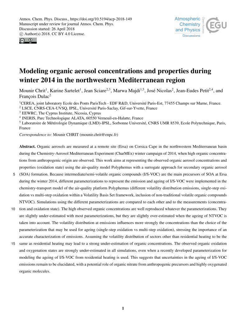
sector "htap_6_residential" of the EDGAR-HTAP_V2 inventory. The emissions from this sector (shown in Figure 1) concern

the emissions from heating/cooling and equipment/lightening of buildings as well as waste treatment. The I/S-VOC emissions

from residential heating are obtained from the POA emissions of sector 6 by multiplying them by a constant factor noted RRH

5


= I/S-VOC/POA. These emissions over the Mediterranean domain are located over big cities (Marseille, Milan, Rome, etc).

I/S-VOC emissions from the six other anthropogenic sources (shown in Figure 1) are estimated from the POA emissions by

multiplying them by a constant factor noted R = I/S-VOC/POA. These emissions are located over big cities and along the main

traffic routes, as well as the shipping routes linking Marseille to Ajaccio and Bastia. Different approaches will also be used to

represent the ageing of I/S-VOC, as described in section 3.5

Figure 1. Surface emissions of POA from the residential heating sector (left panel) and from the other six anthropogenic sectors (right panel)

during the winter 2014. The emissions are in µg.m−2.s−1

2.2 Measurement setup

The ground-based measurements were performed in the framework of ChArMEx (The Chemistry-Aerosol Mediterranean

Experiment) at Ersa (42◦58’N, 9◦21.8’E) on a ridge at the northern tip of Corsica Island at an altitude of about 530 m.a.s.l..

The ground-based comparisons are performed by comparing the measured and modeled concentrations at the model cell the

closest to the station (42◦52N, 9◦22’30”E, 494 m.a.s.l.), as detailed in Chrit et al. (2017). An AerodyneTM ACSM was used10

in order to measure the near real-time mass concetration and chemical composition of aerosols with aerodynamic diameters

between 70 and 1000 nm with a time resolution of 30-min (Ng et al., 2011). This instrument has been continuously running

at Ersa between June 2012 and July 2014 (Nicolas, 2013), with an on-site set-up similar to the one presented in Michoud

et al. (2017). A recent intercomparison exercise, which he ACSM used in this study has successfully taken part in, report an

expanded uncertainty of 19% for OM (Crenn et al., 2015). OM:OC and O:C ratios are estimated using these measurements15

following the methodology provided in Kroll et al. (2011). Although Crenn et al. (2015) and Fröhlich et al. (2015) have shown

consistent results (eg satisfactorily Z-scores) in terms of fragmentation pattern, higher discrepancies were observed for f44

(mass fraction of m/z44), which is an essential variable in the calculation of these elemental ratios. In this respect, results are

presented with an uncertainty which can be estimated as being twice the one of PM (i.e. around 40%).

6


2.3 Model/measurements comparison method

To evaluate the performance of the model, we compare model simulation results to measurements at the Ersa site using a

variety of performance statistical indicators. These indicators are: the simulated mean (s), the root mean square error (RMSE),

the correlation coefficient (corr), the mean fractional bias (MFB) and the mean fractional error (MFE). Table A1 of Appendix

A lists the key statistical indicators definitions used in the model-to-data intercomparison. Furthermore, the criteria of Boylan5

and Russell (2006) (detailed in Table A2 of Appendix A) is used to assess the performance of the simulations.

3 Modeling of I/S-VOC emissions and ageing

In order to understand the behavior of the different parameterizations commonly used in CTMs to represent emissions and

ageing of I/S-VOC in the western Mediterranean region, several simulations using different parameterizations are compared.

These parameterizations are those described in Couvidat et al. (2012), Koo et al. (2014) and Ciarelli et al. (2017b). The10

differences concern the emission ratios used to estimate I/S-VOC from POA (R and RRH ), the ageing scheme (one step or

multi-generational), the modeling of NTVOC, as well as the ratio OM:OC and volatility distribution at emissions.

3.1 One-step oxidation scheme

The one-step oxidation mechanism of Couvidat et al. (2012) is based on the fitting of the curve of dilution of POA from diesel

exhaust of Robinson et al. (2007). I/S-VOC are modeled with three surrogate species POAlP, POAmP and POAhP of different15

volatilities characterized by their saturation concentrations (0.91, 86.21 and 3225.80 µg m−3 respectively). The properties of

the primary and aged I/S-VOC are shown in Table B1 of Appendix B. The ageing of each of these primary surrogates is modeled

by a one-step OH-oxidation reaction in the gas phase (Appendix B), leading to the formation of secondary surrogates SOAlP,

SOAmP and SOAhP. Once formed, these secondary surrogates do not undergo further oxidations. Compared to the primary

surrogates, the volatility of the secondary surrogates is reduced by a factor of 100 and their molecular weight is increased by20

40% (Grieshop et al., 2009; Couvidat et al., 2012) to represent functionalization and fragmentation.

3.2 Multi-generational step oxidation scheme

In sensitivity simulations, for anthropogenic I/S-VOC emissions, the oxidation mechanism is based on the hybrid volatility

basis set (1.5-D VBS) approach developed by Koo et al. (2014). This mechanism combines the simplicity of the 1-dimensional

(1-D) VBS with the ability to describe evolution of OA in the 2-dimensional space of oxidation state and volatility. This25

basis set uses five volatility surrogates, characterized by saturation concentrations varying between 0.1 and 1000 µg m−3. The

surrogates VAP0, VAP1, VAP2, VAP3 and VAP4 refer to the primary surrogates and VAS0, VAS1, VAS2, VAS3 and VAS4

refer to the secondary ones. Table C1 of Appendix C lists their properties.

In the scheme developed by Koo et al. (2014), the OH-oxidation of the primary surrogates leads to a mixture of primary and

secondary surrogates of lower volatility. The carbon (oxygen respectively) number of the lower volatility surrogate decreases30

7


(increases respectively) indicating that functionalization and fragmentation are implicitly accounted for. This mechanism is

detailed in Appendix C.

3.3 Multi-generational step oxidation scheme for residential heating

In sensitivity simulations, for anthropogenic I/S-VOC emissions from residential heating, the VBS model developed by Cia-

relli et al. (2017b) is also used. As in the previously detailed multi-step oxidation scheme, five surrogates with volatilities5

characterized by saturation concentrations extending from 0.1 to 1000 µg m−3 are used. The primary surrogates (BBPOA1,

BBPOA2, BBPOA3, BBPOA4, BBPOA5) react with OH to form secondary surrogates (BBSOA0, BBSOA1, BBSOA2, BB-

SOA3, BBSOA4), whose volatility is one order of magnitude lower than the primary surrogate. In opposition to the one-step

and multi-step oxidation schemes detailed above, here the secondary surrogates may also undergo OH-oxidation forming the

secondary surrogate of lower volatility. As in the other schemes, functionalization and fragmentation are taken into account as10

the carbon and oxygen numbers of the secondary surrogates increases and decreases respectively. The properties of the VBS

surrogates are shown in Table D1 of Appendix D, where reactions are also detailed.

Data from recent wood combustion and ageing experiments performed in smog chamber by Ciarelli et al. (2017b) show

significant contribution of SOA from non-traditional volatile organic compounds (NTVOC: phenol, m-, o-, p-cresol, m-,

o-, p-benzenediol/2-methylfuraldehyde, dimethylphenols, guaiacol/methylbenzenediols, naphthalene, 2-methylnaphthalene/1-15

methylnaphthalene, acenaphthylene, syringol, biphenyl/acenaphthene, dimethylnaphthalene) to OA mass. These NTVOC are

usually not accounted as SOA precursors in CTMs. The NTVOC mixture saturation concentration is estimated to be ∼106

µg m−3 falling with the IVOC saturation concentrations range limit (Koo et al., 2014; Donahue et al., 2012). NTVOC emis-

sions are estimated using a ratio of NTVOC/SVOC of 4.75 (Ciarelli et al., 2017b) and their OH-oxidation produces four

secondary surrogates of different volatilities. These four surrogates may undergo OH-oxidation leading to the less volatile and20

more oxidized secondary surrogate, similarly to the multi-step oxidation described in section 3.3. This mechanism is detailed

in Appendix D and the surrogates properties are listed in Table D2 of Appendix D.

3.4 Volatility distribution and properties of primary emissions

In the one-step oxidation scheme of Couvidat et al. (2012), the emission distribution is based on the fitting of the curve of

dilution of diesel exhaust from Robinson et al. (2007) and is shown in Table 1. This emission distribution is approximately25

similar to the one measured by May et al. (2013a) for biomass burning, and used in the multi-step oxidation scheme for resi-

dential heating of Ciarelli et al. (2017b). In the multi-step oxidation scheme of Koo et al. (2014) for anthropogenic emissions,

the emission distribution is obtained from averaging the emission distributions from gasoline and diesel vehicles measured

by May et al. (2013b, c). As shown in Table 1, the emitted I/S-VOC are less volatile than in the biomass-burning volatility

distribution of May et al. (2013b). Here, the volatility distributions are assigned to a profile number (equal to 1 or 2), depending30

on whether the volatility profile is similar to the profile from biomass burning emissions of May et al. (2013b) (profile number

8


Profil N◦ 1 2 1 2

Reference May et al. (2013b, c) Couvidat et al. (2012) May et al. (2013b, c) May et al. (2013a)

Satu

ratio

nC

onc. 0.9 0.35 0.25

Satu

ratio

nC

onc.

0.1 0.15 0.20

1 0.20 0.10

86.2 0.51 0.3210 0.31 0.10

100 0.20 0.20

3225.8 0.14 0.43 1000 0.14 0.4

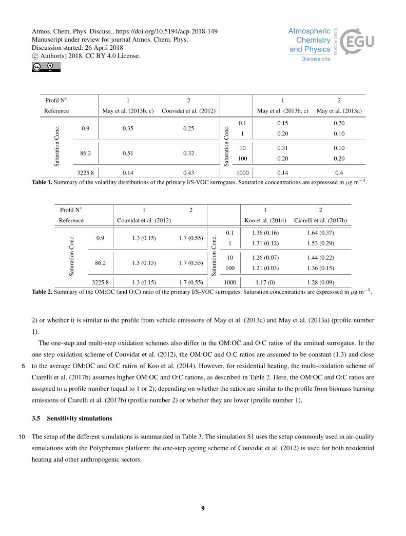
Table 1. Summary of the volatility distributions of the primary I/S-VOC surrogates. Saturation concentrations are expresssed in µg m−3.

Profil N◦ 1 2 1 2

Reference Couvidat et al. (2012) Koo et al. (2014) Ciarelli et al. (2017b)

Satu

ratio

nC

onc. 0.9 1.3 (0.15) 1.7 (0.55)

Satu

ratio

nC

onc.

0.1 1.36 (0.16) 1.64 (0.37)

1 1.31 (0.12) 1.53 (0.29)

86.2 1.3 (0.15) 1.7 (0.55)10 1.26 (0.07) 1.44 (0.22)

100 1.21 (0.03) 1.36 (0.15)

3225.8 1.3 (0.15) 1.7 (0.55) 1000 1.17 (0) 1.28 (0.09)

Table 2. Summary of the OM:OC (and O:C) ratio of the primary I/S-VOC surrogates. Saturation concentrations are expresssed in µg m−3.

2) or whether it is similar to the profile from vehicle emissions of May et al. (2013c) and May et al. (2013a) (profile number

1).

The one-step and multi-step oxidation schemes also differ in the OM:OC and O:C ratios of the emitted surrogates. In the

one-step oxidation scheme of Couvidat et al. (2012), the OM:OC and O:C ratios are assumed to be constant (1.3) and close

to the average OM:OC and O:C ratios of Koo et al. (2014). However, for residential heating, the multi-oxidation scheme of5

Ciarelli et al. (2017b) assumes higher OM:OC and O:C rations, as described in Table 2. Here, the OM:OC and O:C ratios are

assigned to a profile number (equal to 1 or 2), depending on whether the ratios are similar to the profile from biomass burning

emissions of Ciarelli et al. (2017b) (profile number 2) or whether they are lower (profile number 1).

3.5 Sensitivity simulations

The setup of the different simulations is summarized in Table 3. The simulation S1 uses the setup commonly used in air-quality10

simulations with the Polyphemus platform: the one-step ageing scheme of Couvidat et al. (2012) is used for both residential

heating and other anthropogenic sectors.

9


Residential heating Other anthropogenic sectors

Simulation AgeingVolatility

RRH

OM:OCNTVOC Ageing

Volatility R OM:OC

profile profile profile profile

S1 one-step (Couvidat) 2 1.5 1 No one-step (Couvidat) 2 1.5 1


S3 multi-step (Ciarelli) 2 1.5 2 No multi-step (Koo) 1 1.5 1

S4 multi-step (Ciarelli) 2 1.5 2 Yes multi-step (Koo) 1 1.5 1


S6 multi-step (Ciarelli) 2 4.0 2 Yes multi-step (Koo) 1 1.5 1Table 3. Summary of the parameters used in the different simulations performed.

The simulation S2 is conducted to evaluate the impact of the volatility distribution of emissions. Instead of using a volatility

distribution specific of biomass burning for all sectors as in S1, the volatility distribution specific of car emissions is used for

anthropogenic sectors other than residential heating.

The simulation S3 is conducted to evaluate the impact of the ageing scheme. The volatility distributions are similar as S2,

but multi-generational schemes are used rather than a single-oxidation strep for all anthropogenic sectors.5

The simulation S4 is evaluated to estimate the impact of NTVOC. It has the same setup as S2 with multi-generational ageing,

but NTVOC are taken into account.

The simulations S5 and S6 are conducted to assess the impact of the I/S-VOC/POA ratio used for residential heating (RRH ).

The simulation S5 has the same setup as the simulation S2 (single-step oxidation), but it differs in the ratio RRH , which is

assumed to be equal to 4 rather than 1.5. The simulation S6 has the same setup as the simulation S4 (multi-step oxidation and10

NTVOC), but it differs in the ratio RRH , which is assumed to be equal to 4 rather than 1.5.

In terms of the OM:OC ratio, the ratio specific of car emissions is used for emissions from anthropogenic sectors other

than residential heating. For residential heating, higher OM:OC ratios are used in all simulations, except in S1, where the ratio

specific of car emissions is used for all sectors.

4 Organic concentrations15

The spatial distribution of OM1 concentrations averaged over the first 3 months of 2014 (Figure E1 of Appendix E) shows that

high OM1 concentrations are mostly located over big cities like Marseille, Genoa, Turin, Milan, Rome and Naples and along

maritime traffic routes, stressing that organics during wintertime are likely to be mostly of anthropogenic origins.

The simulated composition of OM1 at Ersa is shown in Figure 2 for the simulations S4 and S5. In all simulations, primary

and secondary organic aerosols (POA and SOA) from anthropogenic I/S-VOC are the main components of the organic mass20

(between 60% and 84%). POA tends to account for almost the same fraction of the organic mass than SOA (between 46% and

62%). Similarly, in the U.S., Koo et al. (2014) found that the SOA account for less than half of the modeled OA mass in winter

10


2005 due to the slow chemical ageing during the cold season. Over Europe, in March 2009, Ciarelli et al. (2017a) simulated

that POA accounts between 12 and 68% of the OA, with an average value of 38%. The emission sector 6 (residential heating)

has a large contribution to OA (between 31% and 33%). This is also in line with Ciarelli et al. (2017a) who found that over

Europe in March 2009, the contribution of the residential sector to OA varies between 20% and 45% with an average value of

38%. Furthermore, this sector contributes more to SOA (between 42% and 52% of SOA from I/S-VOC) than to POA (between5

17% and 31% of SOA from I/S-VOC), because their I/S-VOC emissions are more volatile. The contribution from aromatic

VOC is low (lower than 3%), and when NTVOC are considered, they represent between 18% and 21% of the organic mass.

The model simulations performed revealed that, for the winter of 2014, the biogenic OA fraction is low (15-18%). Ciarelli

et al. (2017a) also estimated the biogenic contribution to the organic budget to be between 5 and 20% over Europe.

Figure 2. Simulated composition of OM1 during the winter campaign of 2014 for two simulations: S4 (left panel) and S5 (right panel).

The statistical evaluation of the simulations is shown in Table 4. The performance criterion is satisfied for all simulations10

and the goal criterion is satisfied for S2, S3, S4 and S5. The goal criterion is not satisfied for the simulation S1, which uses

single-step oxidation with a biomass-burning type volatility distribution for all anthropogenic sectors, and for the simulation

S6, which uses multi-step oxidation with NTVOC and a high RRH ratio. The simulation S1 strongly under-estimates the OM1

concentration at Ersa, whereas the simulation S6 strongly over-estimates it.

All the simulations tend to under-estimate the OM1 concentrations at Ersa, except for the two simulations where NTVOC15

are taken into account (S4 and S6), which over-estimate the OM1 concentrations at Ersa.

The model-to-measurement correlation is high for all simulations (between 76 and 83%).

Other CTMs showed the same under-estimation of OM1 concentrations during winter over Europe, even when I/S-VOC

emissions are taken into account (Couvidat et al., 2012; Denier van der Gon et al., 2015). The CTM CAMX (Comprehensive

Air Quality Model with extensions) also under-estimated the organic concentrations over Europe during February and March20

11


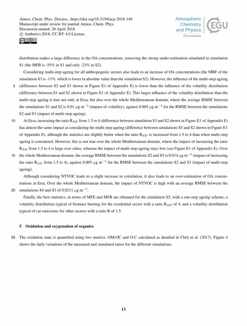
Simulations S1 S2 S3 S4 S5 S6

o=

1.45

s ± RMSE 0.75 ± 1.14 1.06 ± 0.91 1.20 ± 0.85 1.65 ± 0.79 1.25 ± 0.80 2.06 ± 1.08

Correlation (%) 78.3 76.7 76.2 82.4 78.8 82.7

MFB (%) -55 -23 -11 17 -7 38

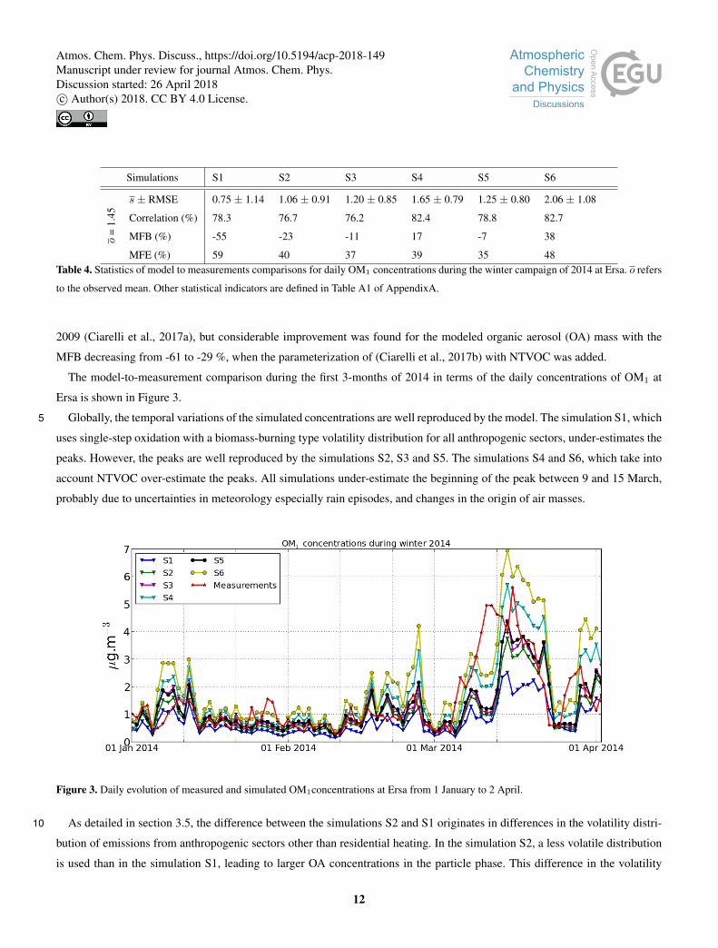
MFE (%) 59 40 37 39 35 48Table 4. Statistics of model to measurements comparisons for daily OM1 concentrations during the winter campaign of 2014 at Ersa. o refers

to the observed mean. Other statistical indicators are defined in Table A1 of AppendixA.

2009 (Ciarelli et al., 2017a), but considerable improvement was found for the modeled organic aerosol (OA) mass with the

MFB decreasing from -61 to -29 %, when the parameterization of (Ciarelli et al., 2017b) with NTVOC was added.

The model-to-measurement comparison during the first 3-months of 2014 in terms of the daily concentrations of OM1 at

Ersa is shown in Figure 3.

Globally, the temporal variations of the simulated concentrations are well reproduced by the model. The simulation S1, which5

uses single-step oxidation with a biomass-burning type volatility distribution for all anthropogenic sectors, under-estimates the

peaks. However, the peaks are well reproduced by the simulations S2, S3 and S5. The simulations S4 and S6, which take into

account NTVOC over-estimate the peaks. All simulations under-estimate the beginning of the peak between 9 and 15 March,

probably due to uncertainties in meteorology especially rain episodes, and changes in the origin of air masses.

Figure 3. Daily evolution of measured and simulated OM1concentrations at Ersa from 1 January to 2 April.

As detailed in section 3.5, the difference between the simulations S2 and S1 originates in differences in the volatility distri-10

bution of emissions from anthropogenic sectors other than residential heating. In the simulation S2, a less volatile distribution

is used than in the simulation S1, leading to larger OA concentrations in the particle phase. This difference in the volatility

12


distribution makes a large difference in the OA concentrations, removing the strong under-estimation simulated in simulation

S1 (the MFB is -55% in S1 and only -23% in S2).

Considering multi-step ageing for all anthropogenic sectors also leads to an increase of OA concentrations (the MBF of the

simulation S3 is -11%, which is lower in absolute value than the simulation S2). However, the influence of the multi-step ageing

(difference between S2 and S3 shown in Figure E1 of Appendix E) is lower than the influence of the volatility distribution5

(difference between S1 and S2 shown in Figure E1 of Appendix E). This larger influence of the volatility distribution than the

multi-step ageing is true not only at Ersa, but also over the whole Mediterranean domain, where the average RMSE between

the simulations S1 and S2 is 0.01 µg m−3 (impact of volatility), against 0.005 µg m−3 for the RMSE between the simulations

S2 and S3 (impact of multi-step ageing).

At Ersa, increasing the ratio RRH from 1.5 to 4 (difference between simulation S3 and S2 shown in Figure E1 of Appendix E)10

has almost the same impact as considering the multi-step ageing (difference between simulations S5 and S2 shown in Figure E1

of Appendix E), although the statistics are slightly better when the ratio RRH is increased from 1.5 to 4 than when multi-step

ageing is considered. However, this is not true over the whole Mediterranean domain, where the impact of increasing the ratio

RRH from 1.5 to 4 is large over cities, whereas the impact of multi-step ageing stays low (see Figure E1 of Appendix E). Over

the whole Mediterranean domain, the average RMSE between the simulations S2 and S5 is 0.014 µg m−3 (impact of increasing15

the ratio RRH from 1.5 to 4), against 0.005 µg m−3 for the RMSE between the simulations S2 and S3 (impact of multi-step

ageing).

Although considering NTVOC leads to a slight increase in correlation, it also leads to an over-estimation of OA concen-

trations at Ersa. Over the whole Mediterranean domain, the impact of NTVOC is high with an average RMSE between the

simulations S4 and S3 of 0.0211 µg m−3.20

Finally, the best statistics, in terms of MFE and MFB are obtained for the simulation S5, with a one-step ageing scheme, a

volatility distribution typical of biomass burning for the residential sector with a ratio RRH of 4, and a volatility distribution

typical of car emissions for other sectors with a ratio R of 1.5.

5 Oxidation and oxygenation of organics

The oxidation state is quantified using two metrics: OM:OC and O:C calculated as detailed in Chrit et al. (2017). Figure 425

shows the daily variations of the measured and simulated ratios for the different simulations.

13


Figure 4. Daily evolution of the ratios OM:OC (left panel) and O:C (right panel) from 01 January to 02 April 2014 at Ersa.

The measurements at Ersa show highly oxidized and oxygenated organics: the measured OM:OC and O:C ratios at Ersa

are respectively 2.21 ± 0.09 and 0.82 ± 0.07 These values are lower than the index measured during the summer 2013 by

Chrit et al. (2017) (2.43 ± 0.07 and 0.99 ± 0.06 for the measured OM:OC and O:C ratios at Ersa respectively), due to the

slower oxidation process owing to the lower temperatures during winter. The average simulated OM:OC and O:C ratios are

shown in Table 5. Both index are strongly underestimated by all simulations, due to the high contribution of POA to the OM15

concentrations (POA is less volatile and oxygenated than SOA). The simulations using multi-step ageing schemes for I/S-VOC

emissions have higher OM:OC and O:C ratios, although the differences are very low (the OM:OC ratio is 1.69 ± 0.53 in S2

(single-step) and 1.72 ± 0.50 in S3 (multi-step). Organics in the simulations where the strength of I/S-VOC emission from

residential heating was increased (simulations S5 and S6) have higher OM:OC and O:C ratios because POA and SOA from

I/S-VOC from residential heating are more oxidized and oxygenated than POA and SOA from other anthropogenic sources.10

Similarly, organics in the simulations where NTVOC are taken into account have higher OM:OC and O:C ratios, because in

the model, NTVOC lead to very oxidized and oxygenated OA. However, the simulated ratios OM:OC and O:C stay under-

estimated (1.85 ± 0.38 and 0.60 ± 0.24 at most, against 2.21 ± 0.09 and 0.82 ± 0.07 in the measurements).

Simulations S1 S2 S3 S4 S5 S6 Measurements

OM:OC 1.60 ± 0.62 1.69 ± 0.53 1.72 ± 0.50 1.85 ± 0.38 1.74 ± 0.49 1.85 ± 0.38 2.21 ± 0.09

O:C 0.38 ± 0.45 0.47 ± 0.36 0.50 ± 0.33 0.60 ± 0.23 0.53 ± 0.31 0.59 ± 0.24 0.82 ± 0.07Table 5. Daily averages of OM:OC and O:C ratios at Ersa during winter 2014 for different simulations. The average measured OM:OC ratio

is 2.21 and the average measured O:C ratio is 0.82.

14


6 Conclusion

This study shows a ground-based comparison of both modeled organic concentrations and properties to measurements per-

formed at Ersa (Cape Corsica, France) during the winter 2014. This work aims at evaluating how commonly used param-

eterizations and assumptions of intermediate/semi-volatile organic compound (I/S-VOC) emissions and ageing perform in

modeling the organic aerosol (OA) concentrations and properties in the western Mediterranean region in winter. To that end,5

the chemistry-transport model from the air quality platform Polyphemus is used with different parameterizations of I/S-VOC

emissions and ageing (different volatility distribution emissions, single-step oxidation vs multi-step oxidation within a Volatil-

ity Basis Set framework, including non-traditional volatile organic compounds NTVOC). Winter (JFM) 2014 simulations are

performed and compared to measurements obtained with an ACSM at the background station of Ersa in the North of Corsica

Island. In all simulations, OA at Ersa is mainly from anthropogenic sources (15 to 18% of OA is from biogenic sources). The10

emission sector 6 (residential heating) has a large contribution to OA (between 31 and 33%). The contribution from aromatic

VOC is low (lower than 3%). NTVOC, as modeled with the parameterization of Ciarelli et al. (2017b) represent between 18%

and 21% of the organic mass. For most simulations, the concentrations of OA compare well to the measurements. All the

simulations tend to under-estimate the OA concentrations at Ersa, except for the two simulations where NTVOC are taken into

account, which, however, over-estimate the OA concentrations. Over the whole western Mediterranean domain, the volatility15

distribution at the emission influences more strongly the concentrations than the choice of the parameterization that may be

used for ageing (single-step oxidation vs multi-step oxidation). Modifying the volatility distribution of sectors other than resi-

dential heating leads to a decrease of 29% in OA concentrations at Ersa, while using the multi-step oxidation parameterization

rather than the single-step one leads to an increase of 13%. The best statistics are obtained using two configurations: the first

one is a one-step ageing scheme, a volatility distribution typical of biomass burning for the residential sector with a ratio I/S-20

VOC/POA at emission of 4, and the second one is a multi-generational ageing scheme, a volatility distribution typical of car

emissions for other sectors with a ratio R I/S-VOC/POA at emission of 1.5.

Both the OM:OC and O:C ratios are underestimated at Ersa in all simulations. The largest simulated OM:OC ratio is equal

to 1.85± 0.83, against 2.21± 0.09 in the measurements. For the summer campaign, Chrit et al. (2017) improved the simulated

OM:OC ratio by adding the formation mechanisms of both extremely-low volatile organic compounds and organic nitrate25

from monoterpene oxidation. Similarly, the formation of organic nitrate and highly oxygenated organic molecules (Molteni

et al., 2018) from aromatic precursors should be added in order to better reproduce the observed OA oxidation/oxygenation

levels. However, adding these new OA formation pathways may lead to an increase in OA concentrations, suggesting that the

actual parameterizations, particularly those with NTVOC may need to be revisited, for example by better characterizing their

deposition.30

Acknowledgements. This research was funded by the French National Research Agency (ANR) projects SAF-MED (grant ANR-12-BS06-

0013). It is part of the ChArMEx project supported by ADEME, CNRS-INSU, CEA and Météo-France through the multidisciplinary pro-

gramme MISTRALS (Mediterranean Integrated Studies aT Regional And Local Scales). It contributes to ChArMEx work packages 1 and 2

15


on emissions and aerosol ageing, respectively. The ACSM at Ersa was funded by the CORSiCA project funded by the Collectivité Territo-

riale de Corse through the Fonds Européen de Développement Régional of the European Operational Program 2007-2013 and the Contrat

de Plan Etat-Région. Eric Hamounou is acknowledged for his great help in setting up the Ersa station. CEREA is a member of the Institut

Pierre-Simon Laplace (IPSL).

16


References

Aiken, A., DeCarlo, P., Krol, J., Worsno, D., Huffma, J., Docherty, K., Ulbrich, I., Mohr, C., Kimmel, J., Sueper, D., Sun, Y., Zhang, Q.,

Trimborn, A., Northway, M., Ziemann, P., Canagaratna, M., Onasch, T., Alfarra, M., Prevot, A., Dommen, J., Duplissy, J., Metzger, A.,

Baltensperger, U., and Jimenez, J.: O/C and OM/OC Ratios of Primary, Secondary, and Ambient Organic Aerosols with High-Resolution

Time-of-Flight Aerosol Mass Spectrometry., Environ. Sci. Technol., 42, 4478–4485, doi:10.1021/es703009q, 2008.5

Bergström, R., Denier van der Gon, H., Prévôt, A., Yttri, K., and Simpson, D.: Modelling of organic aerosols over Europe (2002-2007) using

a volatility basis set (VBS) framework: application of different assumptions regarding the formation of secondary organic aerosol., Atmos.

Chem. Phys., 12, 8499–8527, doi:10.5194/acp-12-8499-2012, 2012.

Boylan, J. W. and Russell, A. G.: PM and light extinction model performance metrics, goals, and criteria for three-dimensional air quality

models, Atmos. Environ., 40, 4946–4959, doi:10.1016/j.atmosenv.2005.09.087, 2006.10

Byun, D. and Ching, J.: Science algorithms of the EPA Models-3 Community Multiscale Air Quality (CMAQ) Modeling System, environ-

mental Protection Agency, Research Triangle Park, NC, 1999.

Canonaco, F., Slowik, J. G., Baltensperger, U., and Prévôt, A. S. H.: Seasonal differences in oxygenated organic aerosol composition:

implications for emissions sources and factor analysis, Atmos. Chem. Phys., 15, 6993–7002, doi:10.5194/acp-15-6993-2015, 2015.

Cappa, C. D. and Jimenez, J. L.: Quantitative estimates of the volatility of ambient organic aerosol, Atmos. Chem. Phys., 10(12), 5409–5424,15

doi:10.5194/acp-10-5409-2010, 2010.

Cholakian, A., Beekmann, M., Colette, A., Coll, I., Siour, G., Sciare, J., Marchand, N., Couvidat, F., Pey, J., Gros, V., Sauvage, S., Michoud,

V., Sellegri, K., Colomb, A., Sartelet, K., Langley Dewitt, H., Elser, M., Prévôt, A. S. H., Szidat, S., and Dulac, F.: Simulation of organic

aerosols in the western Mediterranean area during the ChArMEx 2013 summer campaign, Atmos. Chem. Phys. Discuss., doi:10-51947acp-

2017-697, 2017.20

Chrit, M., Sartelet, K., Sciare, J., Pey, J., Marchand, N., Couvidat, F., Sellegri, K., and Beekmann, M.: Modelling organic aerosol concentra-

tions and properties during ChArMEx summer campaigns of 2012 and 2013 in the western Mediterranean region, Atmos. Chem. Phys.,

17, 12 509–12 531, doi:10.5194/acp-17-12509-2017, 2017.

Ciarelli, G., Aksoyoglu, S., El Haddad, I., Bruns, E. A., Crippa, M., Poulain, L., Äijälä, M., Carbone, S., Freney, E., O’Dowd, C., Bal-

tensperger, U., and Prévôt, A. S. H.: Modelling winter organic aerosol at the European scale with CAMx: valuation and source appor-25

tionment with a VBS parameterization based on novel wood burning smog chamber experiments, Atmos. Chem. Phys., 17, 7653–7669,

doi:10.5194/acp-17-7653-2017, 2017a.

Ciarelli, G., El Haddad, I., Bruns, E., Aksoyoglu, S., Möhler, O., Baltensperger, U., and Prévôt, A. S. H.: Constraining a hybrid volatility

basis-set model for aging of wood-burning emissions using smog chamber experiments: a box-model study based on the VBS scheme of

the CAMx model (v5.40), Geosci. Model Dev., 10, 2303–2320, doi:10.5194/gmd-10-2303-2017, 2017b.30

Couvidat, F. and Sartelet, K.: The Secondary Organic Aerosol Processor (SOAP v1.0) model: a unified model with different ranges of

complexity based on the molecular surrogate approach, Geosci. Model Dev., 8, 1111–1138, doi:10.5194/gmd-8-1111-2015, 2015.

Couvidat, F., Debry, É., Sartelet, K., and Seigneur, C.: A hydrophilic/hydrophobic organic (H2O) model: Model development, evaluation and

sensitivity analysis, J. Geophys. Res., 117, D10 304, doi:10.1029/2011JD017214, 2012.

Couvidat, F., Kim, Y., Sartelet, K., Seigneur, C., Marchand, N., and Sciare, J.: Modeling secondary organic aerosol in an urban area: appli-35

cation to Paris, France, Atmos. Chem. Phys., 13, 983–996, doi:10.5194/acp-13-983-2013, 2013a.

17


Couvidat, F., Sartelet, K., and Seigneur, C.: Investigating the impact of aqueous-phase chemistry and wet deposition on organic aerosol

formation using a molecular surrogate modeling approach, Environ. Sci. Technol., 47, 914–922, doi:10.1021/es3034318, 2013b.

Couvidat, F., Bessagnet, B., Garcia-Vivanco, M., Real, E., Menut, L., and Colette, A.: Development of an inorganic and organic aerosol model

(Chimere2017 β v1.0): seasonal and spatial evaluation over Europe., Geosci. Model Dev. Discuss., in review, doi:doi.org/10.5194/gmd-

2017-120, 2017.5

Crenn, V., Sciare, J., Croteau, P. L., Verlhac, S., Fröhlich, R., Belis, C. A., Aas, W., Äijälä, M., Alastuey, A., Artiñano, B., Baisnée, D.,

Bonnaire, N., Bressi, M., Canagaratna, M., Canonaco, F., Carbone, C., Cavalli, F., Coz, E., Cubison, M. J., Esser-Gietl, J. K., Green, D. C.,

Gros, V., Heikkinen, L., Herrmann, H., Lunder, C., Minguillón, M. C., Mocnik, G., O’Dowd, C. D., Ovadnevaite, J., Petit, J.-E., Petralia,

E., Poulain, L., Priestman, M., Riffault, V., Ripoll, A., Sarda-Estève, R., Slowik, J. G., Setyan, A., Wiedensohler, A., Baltensperger, U.,

Prévôt, A. S. H., Jayne, J. T., , and Favez, O.: ACTRIS ACSM intercomparison – Part 1: Reproducibility of concentration and fragment10

results from 13 individual Quadrupole Aerosol Chemical Speciation Monitors (Q-ACSM) and consistency with co-located instruments,

Atmos. Meas. Tech., 8, 5063–5087, doi:10.5194/amt-8-5063-2015, 2015.

Crippa, M., Canonaco, F., Lanz, V., Äijälä, M., Allan, J., Carbone, S., Capes, G., Ceburnis, D., Dall’Osto, M., Day, A., DeCarlo, P., Ehn, M.,

Eriksson, A., Freney, E., Hildebrandt Ruiz, L., Hillamo, R., Jimenez, J., Junninen, H., Kiendler-Scharr, A., Kortelainen, A.-M., Kulmala,

M., Laaksonen, A., Mensah, A., Mohr, C., Nemitz, E., O’Dowd, C., Ovadnevaite, J., Pandis, S., Petäja, T., Poulain, L., Saarikoski, S.,15

Sellegri, K., Swietlicki, E., Tiitta, P., Worsnop, D., Baltensperger, U., and Prévôt, A.: Organic aerosol components derived from 25

AMS data sets across Europe using a consistent ME-2 based source apportionment approach., Atmos. Chem. Phys., 14, 6159–6176,

doi:10.5194/acp-14-6159-2014, 2014.

Dawson, M., Xu, J., Griffin, R., and Dabdub, D.: Development of aroCACM/MPMPO 1.0: a model to simulate secondary organic aerosol

from aromatic precursors in regional models., Geosci. Model Dev., 9, 2143–2151, doi:10.5194/gmd-9-2143-2016, 2016.20

Debry, É., Fahey, K., Sartelet, K., Sportisse, B., and Tombette, M.: Technical Note: A new SIze REsolved Aerosol Model (SIREAM), Atmos.

Chem. Phys., 7, 1537–1547, doi:10.5194/acp-7-1537-2007, 2007.

Denier van der Gon, H. A. C., Bergström, R., Fountoukis, C., Johansson, C., Pandis, S., Simpson, D., and Visschedijk, A.: Particulate

emissions from residential wood combustion in Europe: revised estimates and an evaluation, Atmos. Chem. Phys., 15, 6503–6519,

doi:10.5194/acp-15-6503-2015, 2015.25

Donahue, N. M., Robinson, A. L., Stanier, C. O., and Pandis, S. N.: Coupled partitioning, dilution, and chemical aging of semivolatile

organics, Environ. Sci. Technol., 40, 2635–2643, doi:10.1021/es052297c, 2006.

Donahue, N. M., Kroll, J. H., Pandis, S. N., and Robinson, A. L.: A two-dimensional volatility basis set – Part 2: Diagnostics of organic-

aerosol evolution, Atmos. Chem. Phys., 12, 615–634, doi:10.5194/acp-12-615-2012, 2012.

Duplissy, J., DeCarlo, P. F., Dommen, J., Alfarra, M. R., Metzger, A., Barmpadimos, I., Prévôt, A. S. H., Weingartner, E., Tritscher, T.,30

Gysel, M., Aiken, A. C., Jimenez, J. L., Canagaratna, M. R., Worsnop, D. R., Collins, D. R., Tomlinson, J., and Baltensperger, U.:

Relating hygroscopicity and composition of organic aerosol particulate matter, Atmos. Chem. Phys., 11, 1155–1165, doi:10.5194/acp-11-

1155-2011, 2011.

El Haddad, I., D’Anna, B., Temime-Roussel, B., Nicolas, M., Boreave, A., Favez, O., Voisin, D., Sciare, J., George, C., Jaffrezo, J.-L.,

Wortham, H., , and Marchand, N.: Towards a better understanding of the origins, chemical composition and aging of oxygenated organic35

aerosols: case study of a Mediterranean industrialized environment, Marseille, Atmos. Chem. Phys., 13, 7875–7894, doi:10.5194/acp-13-

7875-2013, 2013.

18


El-Zanan, H., Lowenthal, D., Zielinska, B., Chow, J., and Kumar, N.: Determination of the organic aerosol mass to organic carbon ratio in

IMPROVE samples., Chemosphere, 60, 480–496, doi:10.1016/j.chemosphere.2005.01.005, 2005.

ENVIRON: User’s Guide, Comprehensive Air Quality Model with Extensions (CAMx), Version 5.40, Environ International Corporation,

california, USA, 2011.

Fountoukis, C., Megaritis, A. G., Skyllakou, K., Charalampidis, P. E., Pilinis, C., Denier van der Gon, H. A. C., Crippa, M., Canonaco,5

F., Mohr, C., Prévôt, A. S. H., Allan, J. D., oulain, L., Petäjä, T., Tiitta, P., Carbone, S., Kiendler-Scharr, A., Nemitz, E., O’Dowd, C.,

Swietlicki, E., and Pandis, S. N.: Organic aerosol concentration and composition over -Europe: insights from comparison of regional

model predictions with aerosol mass spectrometer factor analysis, Atmos. Chem. Phys., 14, 9061–9076, doi:10.5194/acp-14-9061-2014,

2014.

Fröhlich, R., Cubison, M. J., Slowik, J. G., Bukowiecki, N., Canonaco, F., Croteau, P. L., Gysel, M., Henne, S., Herrmann, E., Jayne, J. T.,10

Steinbacher, M., Worsnop, D. R., Baltensperger, U., and Prévôt, A. S. H.: Fourteen months of on-line measurements of the non-refractory

submicron aerosol at the Jungfraujoch (3580 m a.s.l.) – chemical composition, origins and organic aerosol sources, Atmos. Chem. Phys.,

15, 11 373–11 398, doi:10.5194/acp-15-11373-2015, 2015.

GENEMIS: Technical Report, EUROTEC, annual report 1993, 1994.

Gentner, D., Jathar, S., Gordon, T., Bahreini, R., Day, D., El Haddad, I., Hayes, P., Pieber, S., Platt, S., de Gouw, J., Goldstein, A., Harley,15

R., Jimenez, J., Prévôt, A., and Robinson, A.: Review of Urban Secondary Organic Aerosol Formation from Gasoline and Diesel Motor

Vehicle Emissions, Environ. Sci. Technol., 51, 1074–1093, doi:10.1021/acs.est.6b04509, 2017.

Grieshop, A. P., Donahue, N. M., and Robinson, A. L.: Laboratory investigation of photochemical oxidation of organic aerosol from wood

fires 2: analysis of aerosol mass spectrometer data, Atmos. Chem. Phys., 9, 2227–2240, doi:10.5194/acp-9-2227-2009, 2009.

Grosjean, D. and Friedlander, S.: Gas-particle distribution factors for organic and other pollutants in the Los Angeles atmosphere., J. Air20

Pollut. Control Assoc., 25, 1038–1044, 1975.

Guenther, A., Karl, T., Harley, P., Wiedinmyer, C., Palmer, P. I., and Geron, C.: Estimates of global terrestrial isoprene emissions using

MEGAN (Model of Emissions of Gases and Aerosols from Nature), Atmos. Chem. Phys., 6, 3181–3210, doi:10.5194/acp-6-3181-2006,

2006.

Hayes, P. L., Carlton, A. G., Baker, K. R., Ahmadov, R., Washenfelder, R. A., Alvarez, S., Rappenglück, B., Gilman, J. B., Kuster, W. C.,25

de Gouw, J. A., Zotter, P., Prévôt, A. S. H., Szidat, S., Kleindienst, T. E., Offenberg, J. H., Ma, P. K., and Jimenez, J. L.: Modeling

the formation and aging of secondary organic aerosols in Los Angeles during CalNex 2010, Atmos. Chem. Phys., 15, 5773–5801,

doi:10.5194/acp-15-5773-2015, 2015.

Horowitz, L. W., Walters, S., Mauzerall, D. L., Emmons, L. K., Rasch, P. J., Granier, C., Tie, X., Lamarque, J.-F., Schultz, M. G., Tyndall,

G. S., Orlando, J. J., and Brasseur, G. P.: A global simulation of tropospheric ozone and related tracers: Description and evaluation of30

MOZART, version 2, J. Geophys. Res., 108, 4784, doi:10.1029/2002JD002853, 2003.

Huffman, J. A., Docherty, K. S., Mohr, C., Cubison, M. J., Ulbrich, I. M., Ziemann, P. J., Onasch, T. B., and Jimenez, J. L.:

Chemically resolved volatility measurements of organic aerosol from different sources, Environ. Sci. Technol., 43(14), 5351–5357,

doi:10.1021/Es803539d, 2009.

Jimenez, J. L., Canagaratna, M. R., Donahue, N. M., Prevot, A. S., Zhang, Q., Kroll, J. H., DeCarlo, P. F., Allan, J. D., Coe, H., Ng, N. L.,35

Aiken, A. C., Docherty, K. D., Ulbrich, I., Grieshop, A. P., Robinson, A. L., Duplissy, J., Smith, J. D., Wilson, K. R., Lanz, V. A., Hueglin,

C., Sun, Y. L., Tian, J., Laaksonen, A., Raatikainen, T., Rautiainen, J., Vaattovaara, P., Ehn, M., Kulmala, M., Tomlinson, J. M., Collins,

D. R., Cubison, M. J., Dunlea, E. J., Huffman, J. A., Onasch, T. B., Alfarra, M. R., Williams, P. I., Bower, K., Kondo, Y., Schneider, J.,

19


Drewnick, F., Borrmann, S., Weimer, S., Demerjian, K., Salcedo, D., Cottrell, L., Griffin, R., Takami, A., Miyoshi, T., Hatakeyama, S.,

Shimono, A., Sun, J. Y., Zhang, Y. M., Dzepina, K., Kimmel, J. R., Sueper, D., Jayne, J. T., Herndon, S. C., Trimborn, A. M., Williams,

L. R., Wood, E. C., Kolb, C. E., Middlebrook, A. M., Baltensperger, U., and Worsnop, D. R.: Evolution of organic aerosols in the

atmosphere, Science, 326, 1525–1529, doi:10.1126/science.1180353, 2009.

Kim, Y., Sartelet, K., and Seigneur, C.: Formation of secondary aerosols: impact of the gas-phase chemical mechanism, Atmos. Chem. Phys.,5

11, 583–598, doi:10.5194/acp-11-583-2011, 2011.

Kim, Y., Sartelet, K., Seigneur, C., Charron, A., Besombes, J.-L., Jaffrezo, J.-L., Marchand, N., and Polo, L.: Effect of measurement

protocol on organic aerosol measurements of exhaust emissions from gasoline and diesel vehicles, Atmos. Environ., 140, 176–187,

doi:10.1016/j.atmosenv.2016.05.045, 2016.

Koo, B., Knipping, E., and Yarwood, G.: 1.5-Dimensional volatility basis set approach for modeling organic aerosol in CAMx and CMAQ,10

Atmos. Environ., 95, 158–164, doi:10.1016/j.atmosenv.2014.06.031, 2014.

Kroll, J. H., Donahue, N. M., Jimenez, J. L., Kessler, S. H., Canagaratna, M., Wilson, K. R., Altieri, K. E., Mazzoleni, L. R., Wozniak, A. S.,

Bluhm, H., Mysak, E. R., Smith, J. D., E., K. C., and Worsnop, D. R.: Carbon oxidation state as a metric for describing the chemistry of

atmospheric organic aerosol, Nature Chem., 3, 133–139, doi:10.1038/NCHEM.948, 2011.

Lipsky, E. M. and Robinson, A. L.: Effects of dilution on fine particle mass and partitioning of semivolatile organics in diesel exhaust and15

wood smoke, Environ. Sci. Technol., 40(1), 155–162, doi:10.1021/Es050319p, 2006.

May, A., Levin, E., Hennigan, C., Riipinen, I., Lee, T., Collett Jr., J., Jimenez, J., Kreidenweis, S., and Robinson, A.: Gas-particle partitioning

of primary organic aerosol emissions: 3. Biomass burning., JournalofGeophysicalResearch, 118, 11 327–11 338, doi:10.1002/jgrd.50828,

2013a.

May, A., Presto, A., Hennigan, C., Nguyen, N., Gordon, T., and Robinson, A.: Gas-particle partitioning of primary organic aerosol emissions:20

(1) gasoline vehicle exhaust, AtmosphericEnvironment, 77, 128–139, doi:10.1016/j.atmosenv.2013.04.060, 2013b.

May, A., Presto, A., Hennigan, C., Nguyen, N., Gordon, T., and Robinson, A.: Gas-particle partitioning of primary organic aerosol emissions:

(2) diesel vehicles, EnvironmentalScienceandTechnology, 47, 8288–8296, doi:10.1021/es400782j, 2013c.

May, A. A., Levin, E. J. T., Hennigan, C. J., Riipinen, I., Lee, T., Collett, J. L., Jimenez, J. L., Kreidenweis, S. M., and Robinson,

A. L.: Gas-particle partitioning of primary organic aerosol emissions: 3. Biomass burning, J. Geophys. Res.-Atmos., 118, 11 327–11 338,25

doi:10.1002/jgrd.50828, 2013d.

Michoud, V., Sciare, J., Sauvage, S., Dusanter, S., Léonardis, T., Gros, V., Kalogridis, C., Zannoni, N., Féron, A., Petit, J.-E., Crenn, V.,

Baisnée, D., Sarda-Estève, R., Bonnaire, N., Marchand, N., DeWitt, H., Pey, J., Colomb, A., Gheusi, F., Szidat, S., Stavroulas, I., Borbon,

A., and Locoge, N.: Organic carbon at a remote site of the western Mediterranean Basin: sources and chemistry during the ChArMEx

SOP2 field experiment, Atmos. Chem. Phys., 17, 8837–8865, doi:10.5194/acp-17-8837-2017, 2017.30

Minguillón, M., Pérez, N., Marchand, N., Bertrand, A., Temime-Roussel, B., Agrios, K., Szidat, S., van Drooge, B., Sylvestre, A., Alastuey,

A., Reche, C., Ripoll, A., Marco, E., Grimalt, J., and Querol, X.: Secondary organic aerosol origin in an urban environment: influence of

biogenic and fuel combustion precursors, Faraday Discuss., 189, 337–359, doi:10.1039/c5fd00182j, 2016.

Molteni, U., Bianchi, F., Klein, F., El Haddad, I., Frege, C., Rossi, M., Dommen, J., , and Baltensperger, U.: Formation of highly oxygenated

organic molecules from aromatic compounds., Atmos. Chem. Phys., doi:10.5194/acp-2016-1126, 2018.35

Murphy, B., Woody, M., Jimenez, J., Carlton, A., Hayes, P., Liu, S., Ng, N., Russell, L., Setyan, A., Xu, L., Young, J., Zaveri, R., Zhang,

Q., and Pye, H.: Semivolatile POA and parameterized total combustion SOA in CMAQv5.2: impacts on source strength and partitioning.,

Atmos. Chem. Phys., 17, 11 107–11 133, doi:10.5194/acp-17-11107-2017, 2017.

20


Murphy, D. M., Cziczo, D. J., Froyd, K. D., Hudson, P. K., Matthew, B. M., Middlebrook, A. M., Peltier, R. E., Sullivan, A., Thom-

son, D. S., and Weber, R. J.: Single-particle mass spectrometry of tropospheric aerosol particles, J. Geophys. Res., 11, 23–32,

doi:10.1029/2006JD007340, 2006.

Nenes, A., Pandis, S. N., and Pilinis, C.: ISORROPIA: A new thermodynamic equilibrium model for multiphase multicomponent inorganic

aerosols, Aquat. Geochem., 4, 123–152, doi:10.1023/A:1009604003981, 1998.5

Ng, N. L., Herndon, S. C., Trimborn, A., Canagaratna, M. R., Croteau, P. L., Onasch, T. B., Sueper, D., Worsnop, D. R., Zhang, Q., Sun, Y. L.,

and Jayne, J. T.: An Aerosol Chemical Speciation Monitor (ACSM) for Routine Monitoring of the Composition and Mass Concentrations

of Ambient Aerosol, Aerosol Sci. Technol., 45, 780–794, doi:10.1080/02786826.2011.560211, 2011.

Nicolas, J.: Caractérisation physico-chimique de l’aérosol troposphérique en Méditerranée : sources et devenir, PhD dissertation, Univ.

Versailles-Saint-Quentin-en-Yvelines, 2013.10

Ots, R., Young, D., Vieno, M., Xu, L., Dunmore, R., Allan, J., Coe, H., Williams, L., Herndon, S., Ng, N., Hamilton, J., Begström, R.,

Di Marco, C., Nemitz, E., Mackenzie, I., Kuenen, J., Green, D., Reis, S., and Heal, M.: Simulating secondary organic aerosol from missing

diesel-related intermediate-volatility organic compound emissions during the Clean Air for London (ClearfLo) campaign., Atmos. Chem.

Phys., 16, 6453–6473, doi:10.5194/acp-16-6453-2016, 2016.

Robinson, A. L., Donahue, N. M., Shrivastava, M. K., Weitkamp, E. A., Sage, A. M., Grieshop, A. P., Lane, T. E., Pierce, J. R.,15

and Pandis, S. N.: Rethinking Organic Aerosols: Semivolatile Emissions and Photochemical Aging, Science, 315, 1259–1262,

doi:10.1126/science.1133061, 2007.

Sartelet, K., Couvidat, F., Seigneur, C., and Roustan, Y.: Impact of biogenic emissions on air quality over Europe and North America, Atmos.

Environ., 53, 131–141, 2012.

Sartelet, K. N., Debry, E., Fahey, K., Roustan, Y., Tombette, M., and Sportisse, B.: Simulation of aerosols and related species20

over Europe with the Polyphemus system. Part I: model-to-data comparison for 2001, Atmos. Environ., 41, 6116–6131,

doi:10.1016/j.atmosenv.2007.04.024, 2007.

Schwier, A. N., Rose, C., Asmi, E., Ebling, A. M., Landing, W. M., Marro, S., Pedrotti, M.-L., Sallon, A., Iuculano, F., Agusti, S., Tsiola,

A., Pitta, P., Louis, J., Guieu, C., Gazeau, F., , and Sellegri, K.: Primary marine aerosol emissions from the Mediterranean Sea during pre-

bloom and oligotrophic conditions: correlations to seawater chlorophyll a from a mesocosm study, Atmos. Chem. Phys., pp. 7961–7976,25

doi:10.5194/acp-15-7961-2015, 2015.

Shrivastava, M., Cappa, C., Fan, J., Goldstein, A., Guenther, A., Jimenez, J., Kuang, C., Laskin, A., Martin, S., Ng, N., Petaja, T., Pierce,

J., Rasch, P., Roldin, P., Seinfeld, J., Shilling, J., Smith, J., Thornton, J., Volkamer, R., Wang, J., Worsnop, D., Zaveri, R., Zelenyuk, A.,

and Zhang, Q.: Recent advances in understanding secondary organic aerosol: Implications for global climate forcing, Rev. Geophys., 55,

509–559, doi:10.1002/2016RG000540, 2017.30

Stockwell, C. E., Veres, P. R., Williams, J., and Yokelson, R. J.: Characterization of biomass burning emissions from cooking fires, peat, crop

residue, and other fuels with high-resolution proton-transfer-reaction time-of-flight mass spectrometry, Atmos. Chem. Phys., 15, 845–865,

doi:10.5194/acp-15-845-2015, 2015.

Troen, I. B. and Mahrt, L.: A simple model of the atmospheric boundary layer; sensitivity to surface evaporation, Bound.-Layer Meteorol.,

37, 129–148, doi:10.1007/BF00122760, 1986.35

Tsimpidi, A. P., Karydis, V. A., Zavala, M., Lei, W., Molina, L., Ulbrich, I. M., Jimenez, J. L., and Pandis, S. N.: Evaluation of the volatility

basis-set approach for the simulation of organic aerosol formation in the Mexico City metropolitan area, Atmos. Chem. Phys., 10, 525–546,

doi:10.5194/acp-10-525-2010, 2010.

21


Turpin, B. and Lim, H.-J.: Species Contributions to PM2.5 Mass Concentrations: Revisiting Common Assumptions for Estimating Organic

Mass., Aerosol Sci. Technol., 35, 602–610, doi:10.1080/02786820119445, 2001.

Wong, J. P. S., Lee, A. K. Y., Slowik, J. G., Cziczo, D. J., Leaitch, W. R., Macdonald, A., and Abbatt, J. P. D.: Oxidation of ambient biogenic

secondary organic aerosol by hydroxyl radicals: Effects on cloud condensation nuclei activity, Geophys. Res. Lett., 38, 22 805–22 811,

doi:10.1029/2011GL04935, 2011.5

Woody, M. C., Baker, K. R., Hayes, P. L., Jimenez, J. L., Koo, B., and Pye, H. O. T.: Understanding sources of organic aerosol during

CalNex-2010 using the CMAQ-VBS, Atmos. Chem. Phys., 16, 4081–4100, doi:10.5194/acp-16-4081-2016, 2016.

Xing, L., Fu, T.-M., Cao, J. J., Lee, S. C., Wang, G. H., Ho, K. F., Cheng, M.-C., You, C.-F., and Wang, T. J.: Seasonal and spatial variability

of the OM/OC mass ratios and high regional correlation between oxalic acid and zinc in Chinese urban organic aerosols, Atmos. Chem.

Phys., 13, 4307–4318, doi:10.5194/acp-13-4307-2013, 2013.10

Zhang, Q., Alfarra, M., Worsnop, D., Allan, J., Coe, H., Canagaratna, M., and Jimenez, J.: Deconvolution and quantification of hydrocarbon-

like and oxygenated organic aerosols based on aerosol mass spectrometry., Environ. Sci. Technol., 39, 4938–4952, doi:10.1021/es048568l,

2005a.

Zhang, Q., Worsnop, D., Canagaratna, M., and Jimenez, J.: Hydrocarbon-like and oxygenated organic aerosols in Pittsburgh: insights into

sources and processes of organic aerosols., Atmos. Chem. Phys., 5, 3289–3311, doi:10.5194/acp-5-3289-2005, 2005b.15

Zhao, Y., Nguyen, N., Presto, A., Hennigan, C., May, A., and Robinson, A.: Intermediate volatility organic compound emissions from on-

road diesel vehicles: chemical composition, emission factors, and estimated secondary organic aerosol production., Environ. Sci. Technol.,

49, 11 516–11 526, doi:10.1021/acs.est.5b02841, 2015.

Zhao, Y., Nguyen, N., Presto, A., Hennigan, C., May, A., and Robinson, A.: Intermediate volatility organic compound emissions from on-road

gasoline vehicles and small off-road gasoline engines., Environ. Sci. Technol., 50, 4554–4563, doi:10.1021/acs.est.5b06247, 2016.20

Zhu, S., Sartelet, K., Healy, R., and Wenger, J.: Simulation of particle diversity and mixing state over Greater Paris: A model-measurement

inter-comparison, Faraday Discuss., 189, 547–566, doi:10.1039/C5FD00175G, 2016.

22


Appendix A: Statistical indicators and criteria

Statistic indicator Definition

Root mean square error (RMSE)

√1

n

∑ni=1(ci− oi)2

Correlation (Corr)∑n

i=1(ci− c)(oi− o)√∑ni=1(ci− c)2

√∑ni=1(oi− o)2

Mean fractional bias (MFB)1

n

∑ni=1

ci− oi

(ci + oi)/2

Mean fractional error (MFE)1

n

∑ni=1

| ci− oi |(ci + oi)/2

Table A1. Definitions of the statistics used in this work. (oi)i and (ci)i are the observed and the simulated concentrations at time and location

i, respectively. n is the number of data

Criteria Performance criterion Goal criterion

|MFB| ≤ 60% ≤ 30%

MFE ≤ 75% ≤ 50%Table A2. Boylan and Russel criteria

23


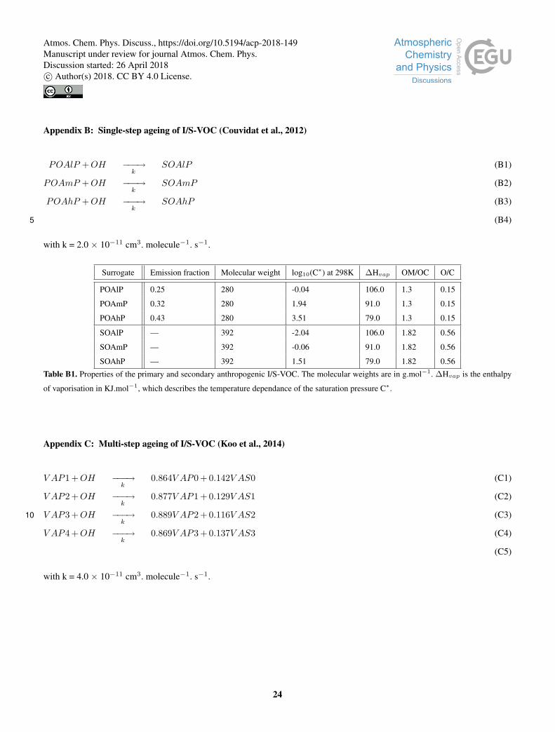
Appendix B: Single-step ageing of I/S-VOC (Couvidat et al., 2012)

POAlP +OH −−−→k

SOAlP (B1)

POAmP +OH −−−→k

SOAmP (B2)

POAhP +OH −−−→k

SOAhP (B3)

(B4)5

with k = 2.0 × 10−11 cm3. molecule−1. s−1.

Surrogate Emission fraction Molecular weight log10(C∗) at 298K ∆Hvap OM/OC O/C

POAlP 0.25 280 -0.04 106.0 1.3 0.15

POAmP 0.32 280 1.94 91.0 1.3 0.15

POAhP 0.43 280 3.51 79.0 1.3 0.15

SOAlP — 392 -2.04 106.0 1.82 0.56

SOAmP — 392 -0.06 91.0 1.82 0.56

SOAhP — 392 1.51 79.0 1.82 0.56

Table B1. Properties of the primary and secondary anthropogenic I/S-VOC. The molecular weights are in g.mol−1. ∆Hvap is the enthalpy

of vaporisation in KJ.mol−1, which describes the temperature dependance of the saturation pressure C∗.

Appendix C: Multi-step ageing of I/S-VOC (Koo et al., 2014)

V AP1 +OH −−−→k

0.864V AP0 +0.142V AS0 (C1)


0.877V AP1 +0.129V AS1 (C2)


0.889V AP2 +0.116V AS2 (C3)10


0.869V AP3 +0.137V AS3 (C4)

(C5)

with k = 4.0 × 10−11 cm3. molecule−1. s−1.

24



VAP0 0.15 278 -1 96.0 1.36 0.16

VAP1 0.20 275 0 85.0 1.31 0.12

VAP2 0.31 272 1 74.0 1.26 0.07

VAP3 0.20 268 2 63.0 1.21 0.03

VAP4 0.14 266 3 55.0 1.17 0.00

VAS0 — 172 -1 35 2.05 0.70

VAS1 — 167 0 35 1.92 0.60

VAS2 — 163 1 35 1.81 0.51

VAS3 — 158 2 35 1.70 0.43

VAS4 — 153 3 35 1.59 0.34

Table C1. Properties of the VBS species (the primary and secondary anthropogenic SVOC). The molecular weights are in g.mol−1. ∆Hvap

is the enthalpy of vaporisation in KJ.mol−1, which describes the temperature dependance of the saturation pressure C∗.

Appendix D: Multi-step ageing of I/S-VOC from residential heating (Ciarelli et al., 2017b)

BBPOA4 +OH −−−→k

BBSOA3 (D1)


BBSOA2 (D2)


BBSOA1 (D3)


BBSOA0 (D4)5

BBSOA3 +OH −−−→k

BBSOA2 (D5)


BBSOA1 (D6)


BBSOA0 (D7)

NTV OC +OH −−−→k

0.143BB3SOA4 +0.097BB3SOA3 +0.069BB3SOA2 +0.011BB3SOA1 (D8)

BB3SOA4 +OH −−−→k

BB3SOA3 (D9)10


BB3SOA2 (D10)


BB3SOA1 (D11)


BB3SOA0 (D12)

(D13)

with k = 4.0 × 10−11 cm3. molecule−1. s−1.15

25



NTVOC 4.75 113 6 — — —

BBPOA0 0.20 216 -1 85.0 1.64 0.37

BBPOA1 0.10 216 0 77.5 1.53 0.29

BBPOA2 0.10 216 1 70.0 1.44 0.22

BBPOA3 0.20 216 2 62.5 1.36 0.15

BBPOA4 0.40 215 3 55.0 1.28 0.09

BBSOA0 — 194 -1 35.0 1.80 0.50

BBSOA1 — 189 0 35.0 1.70 0.43

BBSOA2 — 184 1 35.0 1.61 0.36

BBSOA3 — 179 2 35.0 1.53 0.29

BB3SOA0 — 149 -1 35.0 2.48 1.05

BB3SOA1 — 144 0 35.0 2.29 0.90

BB3SOA2 — 140 1 35.0 2.12 0.76

BB3SOA3 — 135 2 35.0 1.96 0.63

BB3SOA4 — 131 3 35.0 1.82 0.52

Table D1. Properties of the VBS species (the NTVOC and primary and secondary RH-I/S-VOC). The molecular weights are in g.mol−1.

∆Hvap is the enthalpy of vaporisation in KJ.mol−1, which describes the temperature dependance of the saturation pressure C∗.

26



NTVOC 4.75 113 6 — — —

BBPOA0 0.20 216 -1 85.0 1.64 0.37

BBPOA1 0.10 216 0 77.5 1.53 0.29

BBPOA2 0.10 216 1 70.0 1.44 0.22

BBPOA3 0.20 216 2 62.5 1.36 0.15

BBPOA4 0.40 215 3 55.0 1.28 0.09

BBSOA0 — 194 -1 35.0 1.80 0.50

BBSOA1 — 189 0 35.0 1.70 0.43

BBSOA2 — 184 1 35.0 1.61 0.36

BBSOA3 — 179 2 35.0 1.53 0.29

BB3SOA0 — 149 -1 35.0 2.48 1.05

BB3SOA1 — 144 0 35.0 2.29 0.90

BB3SOA2 — 140 1 35.0 2.12 0.76

BB3SOA3 — 135 2 35.0 1.96 0.63

BB3SOA4 — 131 3 35.0 1.82 0.52

Table D2. Properties of the NTVOC and their oxidation products). The molecular weights are in g.mol−1. ∆Hvap is the enthalpy of vapori-

sation in KJ.mol−1, which describes the temperature dependance of the saturation pressure C∗.

27


Appendix E: Maps of OM1 concentrations and differences between simulations.

Figure E1. Maps of the concentrations of OM1 (µg m−3) averaged over January to March 2014 using S1 (upper left panel) and the absolute

difference of OM1 concentrations between S2 and S1 (upper right panel, impact of volatility), S3 and S2 (lower left panel, impact of multi-

step ageing), and S5 and S2 (lower right panel, impact of increasing RRH from 1.5 to 4.

28


Date post:	12-Sep-2018
Category:	Documents
Upload:	phamkhanh
View:	213 times
Download:	0 times

Modeling organic aerosol concentrations and properties ... · 5 Laboratoire de Métérologie...

Documents