Modeling Power Saving for GAN and UMTS

Interworking

Shun-Ren Yang∗, Phone Lin†, and Pei-Tang Huang‡

Abstract

3GPP 43.318 specifies the Generic Access Network (GAN) for interworking between Wire-

less Local Area Network (WLAN) and Universal Mobile Telecommunications System (UMTS)

core network. A dual-mode Mobile Station (MS) is equipped with two communication mod-

ules to support both WLAN and UMTS radio technologies, which shortens the battery

lifetime of the MS. This paper proposes an analytical model and conducts simulation experi-

ments to study the power consumption of dual-mode MSs in terms of the power consumption

indicator and mean packet waiting time. Our study provides guidelines for designing WLAN-

UMTS dual-mode MSs.

Keywords: Generic Access Network (GAN), Power Saving, Universal Mobile Telecommu-

nications System (UMTS), Wireless Local Area Network (WLAN).

1 Introduction

IEEE 802.11 Wireless Local Area Network (WLAN) provides users high bit-rate wireless

transmission service within hot-spot areas, e.g., indoor or basement. On the other hand,

∗Shun-Ren Yang is with Department of Computer Science and Institute of Communications Engineering,

National Tsing Hua University, Hsinchu, Taiwan, R.O.C. Yang’s e-mail address is sryang@cs.nthu.edu.tw.†Corresponding Author: Phone Lin is with Department of Computer Science and Information Engineer-

ing, Graduate Institute of Networking and Multimedia, National Taiwan University, Taipei, Taiwan, R.O.C.

Lin’s e-mail address is plin@csie.ntu.edu.tw.‡Pei-Tang Huang is with Department of Computer Science and Information Engineering, National Taiwan

University, Taipei, Taiwan, R.O.C. Huang’s email address is tang@pcs.csie.ntu.edu.tw.

1

3GPP Universal Mobile Telecommunications System (UMTS) provides wireless transmission

service within wide areas and supports high user mobility. WLAN and UMTS are treated

as complementary wireless network technologies [6]. To provide users wireless access service

to networks irrespective of their locations and network access technologies, the Unlicensed

Mobile Access (UMA) technology [18] is proposed for interworking and integration between

UMTS and WLAN, which has been proven and accommodated in 3GPP 43.318 [1]. The

Generic Access Network (GAN) is defined in 3GPP 43.318 to enable WLAN to connect to

the UMTS core network.

GAN provides UMTS subscribers with the low-cost and high-speed WLAN access. How-

ever, a dual-mode Mobile Station (MS) is equipped with two communication modules for

both WLAN and UMTS radio technologies. The work in [17] showed that the battery life-

time will be significantly shortened while an additional WLAN module is added to an MS.

Therefore, how to reduce dual-mode MS power consumption is an important issue, which

may reflect the user satisfaction with the offered wireless access service. Many research

efforts in the literature have dedicated to the investigation of the MS power saving mecha-

nisms in different wireless mobile networks, e.g., [14] for CDPD, [19] for UMTS, [12] for both

UMTS and cdma2000, and [20] for IEEE 802.11 WLAN. Nevertheless, all of these studies

only considered the power consumption behavior of single-mode MSs. To the best of our

knowledge, there is no previous work covering the “power saving of a dual-mode MS” topic.

This paper proposes an analytical model to study the power consumption issue for MSs

operating in the GAN and UMTS interworking network. The model quantifies the power

consumption of a WLAN-UMTS dual-mode MS, which is referred to as the power consump-

tion indicator. It is clear that the lower the power consumption indicator, the more effective

the utilized power management technique. However, reducing the power consumption may

at the same time degrade the system performance in terms of service delay. Therefore, we

also quantify the mean packet waiting time to examine the penalty caused by exercising the

power saving mechanism for GAN-UMTS interworking. Due to the complicated behavior

of a dual-mode MS, the proposed analytical model may not well capture the MS behavior

under some conditions. To release these constraints of the analytical model, we conduct

simulation experiments as well. We note that the performance of a power saving mechanism

primarily depends on MSs’ uplink and downlink packet transmission/reception behavior.

2

Whenever an MS has uplink packets to transmit, it can immediately terminate the power

saving operation and switch into the power active state for packet delivery. On the other

hand, for the downlink packet reception, it is very difficult for MSs to predict the instants

of the subsequent packet arrivals. In this case, an MS can not adjust its power management

state proactively to adapt to the downlink packet traffic. This paper will concentrate on

the more challenging power management for MS downlink packet transmissions. The uplink

performance metrics such as the transmission power consumption of MSs are therefore not

discussed in this paper. Our work derives close-form equations for both the power consump-

tion indicator and mean packet waiting time with the premise that the WLAN available and

unavailable periods are sufficiently small. Furthermore, our study indicates that with proper

parameter settings, power management techniques can reduce the power consumption indi-

cator of a WLAN-UMTS dual-mode MS without significantly increasing the mean packet

waiting time. The analytical and simulation results of this work can serve as guidelines for

the implementation of WLAN-UMTS dual-mode MSs.

2 System Model

This section first gives an overview of the GAN-UMTS interworking architecture, and then

describes the system model for our study of GAN-UMTS dual-mode MS power saving.

Figure 1 illustrates a simplified system architecture for the GAN-UMTS interworking,

where GAN (Figure 1 (a)) is an alternative radio access network for the UMTS core network

(Figure 1 (d)). We may apply any kind of IP access technologies in GAN, such as IEEE

802.11 [9] or Bluetooth [3]. This paper assumes IEEE 802.11 WLAN (Figure 1 (h)) as the

underlying IP access technology in GAN. Both GAN and UMTS Terrestrial Radio Access

Network (UTRAN; Figure 1 (b)) connect to Serving GPRS Support Node (SGSN; Figure 1

(c)) in the UMTS core network and receive packets destined to a dual-mode MS (Figure 1

(e)) from external IP networks (Figure 1 (j)). Functioning like Radio Network Controller

(RNC; Figure 1 (f)) in UTRAN, Generic Access Network Controller (GANC; Figure 1 (g)) in

GAN receives packets from SGSN and forwards them to the MS through Access Points (APs;

Figure 1 (k)) in WLAN. While the MS leaves WLAN coverage, the SGSN may also forward

the incoming packets to the RNC in the UTRAN. The RNC processor sends the packets to

3

the Node B (Figure 1 (l)) through an Asynchronous Transfer Mode (ATM; Figure 1 (m))

link. The Node B then delivers the packets to the MS through the Wideband Code Division

Multiple Access (WCDMA) radio link.

To conserve the power budget of a GAN-UMTS dual-mode MS, the UMTS Discontinuous

Reception (DRX) [2] and the IEEE 802.11 Power Saving Mode (PSM) [9] are employed,

respectively. The concept of DRX is for an idle MS to power off the radio receiver for

a predefined period (referred as DRX cycle) instead of continuously listening to the radio

channel signal. As shown in Figure 2, the activities of an MS’s UMTS receiver module under

DRX can be characterized in terms of three periods:

Busy periods. During packet transmission to the MS, incoming packets are first stored

in the RNC buffer before they are delivered to the MS. Then, the RNC processor

transmits the packets in the First In First Out (FIFO) order.

Inactivity periods. When the RNC buffer becomes empty, the RNC inactivity timer is

activated. If any packet arrives at the RNC before the inactivity timer expires, the

timer is stopped. The RNC processor starts to transmit packets, and another busy

period begins.

Sleep periods. If no packet arrives before the inactivity timer expires, the MS enters a

sleep period, and the UMTS receiver module is turned off. The sleep period contains

one or more DRX cycles. At the end of a DRX cycle, the MS wakes up to listen to the

paging channel. If some packets have arrived at the RNC during the last DRX cycle,

the MS starts to receive packets and the sleep period ends. Otherwise, the MS returns

to sleep until the end of the next DRX cycle.

Note that during busy and inactivity periods, the MS turns on the UMTS receiver module.

Zheng et al. [20] have shown that the IEEE 802.11 PSM mechanism is oblivious of

the packet traffic characteristics, and thus is not energy-efficient under light traffic load

and suffer from significant performance degradation at higher traffic load in terms of power

consumption and packet mean waiting time. Therefore, our system model considers UMTS

DRX mechanism during packet transmission through UMTS but ignores IEEE 802.11 PSM

during packet transmission through IEEE 802.11 WLAN.

4

As shown in Figure 3, since the WLAN can support higher data transmission rate and

is of lower cost, we suppose that the SGSN delivers the packets to the GANC whenever

possible. The SGSN could also utilize the global always-on UMTS connectivity for packet

delivery when the MS leaves the WLAN hotspot coverage and the WLAN connection is not

available. Suppose that packet arrivals for an MS to the SGSN form a Poisson stream with

rate λa. We assume that the WLAN availability for the MS follows the ON-OFF patterns

repeatedly. Specifically, the WLAN connectivity is available during an ON period, and is

unavailable when the ON period ends. Then, the WLAN connectivity enters an OFF period.

The ON and OFF periods are assumed to be exponentially distributed with rates λo and λf ,

respectively.

Due to the high wireless transmission rate feature of WLAN, we assume that each packet

arrival to the GANC can be transmitted immediately, and no packet has to be buffered in the

GANC. When packets arrive during a WLAN OFF period, they are forwarded to the RNC.

In UTRAN, ATM is much faster and more reliable than the WCDMA wireless transmission.

Therefore, we ignore the ATM transmission delay between the RNC and the Node B, and

the RNC and the Node B are modeled as a FIFO queueing server. Let tx denote the packet

service time, i.e., the interval between the time when a packet is transmitted by the RNC

processor and the time when the corresponding ack is received by the RNC processor. Let

tI be the threshold of the RNC inactivity timer, and tD be the length of the UMTS DRX

cycle. At the end of every DRX cycle, the MS must wake up for a short period τ so that it

can listen to the paging information from the network. Therefore the “power saving” period

in a DRX cycle is tD − τ .

3 An Analytic Model

This section proposes an analytical model to investigate the power consumption of a dual-

mode MS. In the following, we first determine the packet arrival process to the RNC. Then,

based on the inter-packet arrival time distribution to the RNC, we derive the following two

output measures:

• the power consumption indicator Pi: the average power consumption of an MS’s radio

receivers (including the UMTS and the WLAN receiver modules) when the UMTS

5

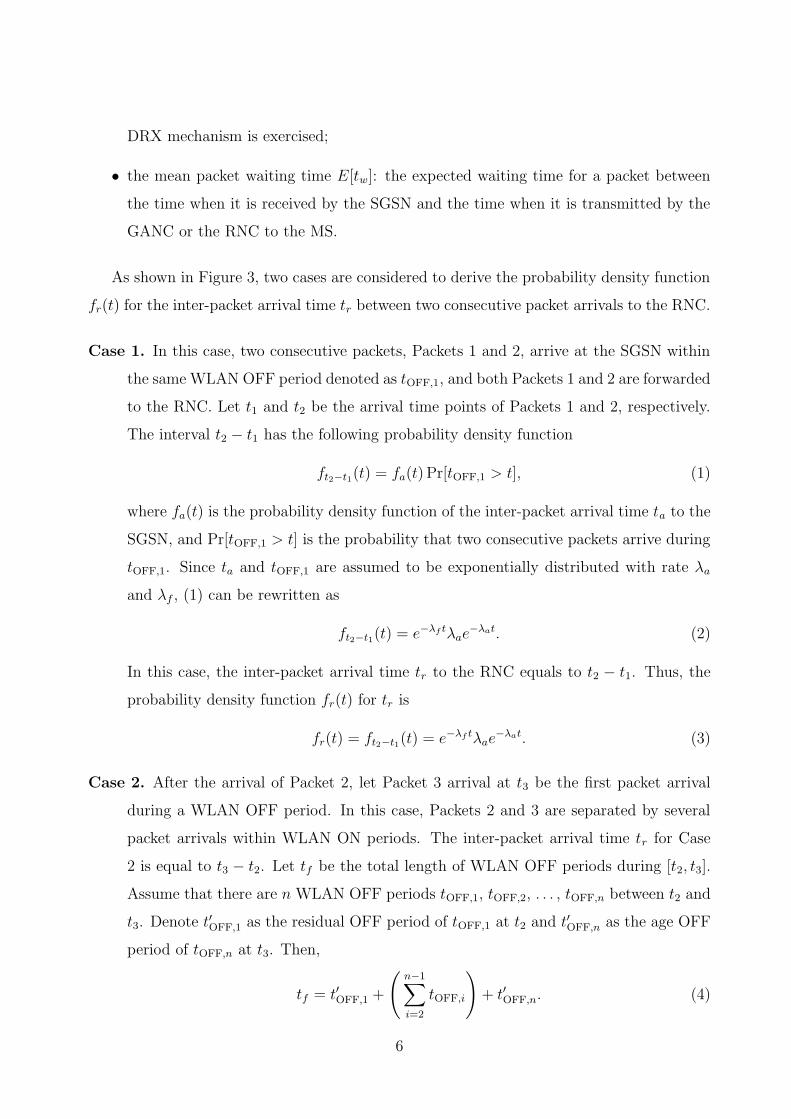
DRX mechanism is exercised;

• the mean packet waiting time E[tw]: the expected waiting time for a packet between

the time when it is received by the SGSN and the time when it is transmitted by the

GANC or the RNC to the MS.

As shown in Figure 3, two cases are considered to derive the probability density function

fr(t) for the inter-packet arrival time tr between two consecutive packet arrivals to the RNC.

Case 1. In this case, two consecutive packets, Packets 1 and 2, arrive at the SGSN within

the same WLAN OFF period denoted as tOFF,1, and both Packets 1 and 2 are forwarded

to the RNC. Let t1 and t2 be the arrival time points of Packets 1 and 2, respectively.

The interval t2 − t1 has the following probability density function

ft2−t1(t) = fa(t) Pr[tOFF,1 > t], (1)

where fa(t) is the probability density function of the inter-packet arrival time ta to the

SGSN, and Pr[tOFF,1 > t] is the probability that two consecutive packets arrive during

tOFF,1. Since ta and tOFF,1 are assumed to be exponentially distributed with rate λa

and λf , (1) can be rewritten as

ft2−t1(t) = e−λf tλae−λat. (2)

In this case, the inter-packet arrival time tr to the RNC equals to t2 − t1. Thus, the

probability density function fr(t) for tr is

fr(t) = ft2−t1(t) = e−λf tλae−λat. (3)

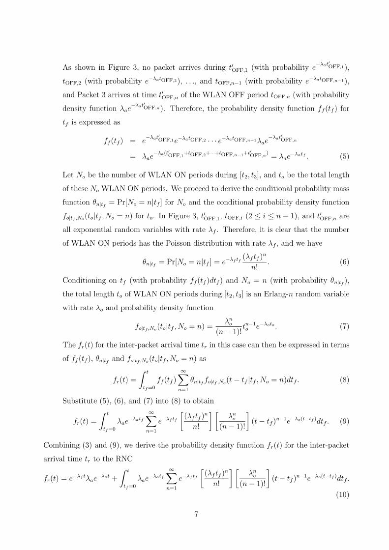
Case 2. After the arrival of Packet 2, let Packet 3 arrival at t3 be the first packet arrival

during a WLAN OFF period. In this case, Packets 2 and 3 are separated by several

packet arrivals within WLAN ON periods. The inter-packet arrival time tr for Case

2 is equal to t3 − t2. Let tf be the total length of WLAN OFF periods during [t2, t3].

Assume that there are n WLAN OFF periods tOFF,1, tOFF,2, . . . , tOFF,n between t2 and

t3. Denote t′OFF,1 as the residual OFF period of tOFF,1 at t2 and t′OFF,n as the age OFF

period of tOFF,n at t3. Then,

tf = t′OFF,1 +

(

n−1∑

i=2

tOFF,i

)

+ t′OFF,n. (4)

6

As shown in Figure 3, no packet arrives during t′OFF,1 (with probability e−λat′

OFF,1),

tOFF,2 (with probability e−λatOFF,2), . . ., and tOFF,n−1 (with probability e−λatOFF,n−1),

and Packet 3 arrives at time t′OFF,n of the WLAN OFF period tOFF,n (with probability

density function λae−λat′

OFF,n). Therefore, the probability density function ff (tf ) for

tf is expressed as

ff (tf ) = e−λat′

OFF,1e−λatOFF,2 · · · e−λatOFF,n−1λae−λat′

OFF,n

= λae−λa(t′

OFF,1+tOFF,2+···+tOFF,n−1

+t′OFF,n

)= λae

−λatf . (5)

Let No be the number of WLAN ON periods during [t2, t3], and to be the total length

of these No WLAN ON periods. We proceed to derive the conditional probability mass

function θn|tf = Pr[No = n|tf ] for No and the conditional probability density function

fo|tf ,No(to|tf , No = n) for to. In Figure 3, t′OFF,1, tOFF,i (2 ≤ i ≤ n− 1), and t′OFF,n are

all exponential random variables with rate λf . Therefore, it is clear that the number

of WLAN ON periods has the Poisson distribution with rate λf , and we have

θn|tf = Pr[No = n|tf ] = e−λf tf(λf tf )

n

n!. (6)

Conditioning on tf (with probability ff (tf )dtf ) and No = n (with probability θn|tf ),

the total length to of WLAN ON periods during [t2, t3] is an Erlang-n random variable

with rate λo and probability density function

fo|tf ,No(to|tf , No = n) =

λno

(n− 1)!tn−1o e−λoto . (7)

The fr(t) for the inter-packet arrival time tr in this case can then be expressed in terms

of ff (tf ), θn|tf and fo|tf ,No(to|tf , No = n) as

fr(t) =

∫ t

tf=0

ff (tf )∞∑

n=1

θn|tf fo|tf ,No(t− tf |tf , No = n)dtf . (8)

Substitute (5), (6), and (7) into (8) to obtain

fr(t) =

∫ t

tf=0

λae−λatf

∞∑

n=1

e−λf tf

[

(λf tf )n

n!

] [

λno

(n− 1)!

]

(t− tf )n−1e−λo(t−tf )dtf . (9)

Combining (3) and (9), we derive the probability density function fr(t) for the inter-packet

arrival time tr to the RNC

fr(t) = e−λf tλae−λat +

∫ t

tf=0

λae−λatf

∞∑

n=1

e−λf tf

[

(λf tf )n

n!

] [

λno

(n− 1)!

]

(t− tf )n−1e−λo(t−tf )dtf .

(10)

7

Equation (10) is too complicated for the analysis of Pi and E[tw]. With the following

theorem, we attempt to obtain a simpler fr(t) probability density function.

Theorem 1 When λo → ∞, λf → ∞ andλf

λo→ C > 0 where C is a constant, we have

that the inter-packet arrival time tr to the RNC follows an exponential distribution with rate

λa

1+C.

Proof. Since No|tf is a Poisson random variable with rate λf (see (6)), we have

E[No|tf ] = λf tf and V ar[No|tf ] = λf tf . (11)

Furthermore, to|tf , No = n is an Erlang-n random variable with rate λo (see (7)), and

therefore

E[to|tf , No = n] =n

λo

and V ar[to|tf , No = n] =n

λ2o

. (12)

Using expectation by conditioning technique [16], we have that

E[to|tf ] = E[E[to|tf , No]|tf ]. (13)

From (11) and (12), (13) is rewritten as

E[to|tf ] = E

[

No

λo

∣

∣

∣

∣

tf

]

=λf tfλo

. (14)

According to [16, page 51], the variance V ar[to|tf ] can be expressed as

V ar[to|tf ] = V ar[E[to|tf , No]|tf ] + E[V ar[to|tf , No]|tf ]. (15)

Substitute (11) and (12) into (15) to yield

V ar[to|tf ] = V ar

[

No

λo

∣

∣

∣

∣

tf

]

+ E

[

No

λ2o

∣

∣

∣

∣

tf

]

=λf tfλ2

o

+λf tfλ2

o

=2λf tf

λ2o

. (16)

From (14) and (16), it is clear that when λo → ∞, λf → ∞ andλf

λo→ C, E[to|tf ] → Ctf

and V ar[to|tf ]→ 0, that is, to|tf converges to a constant Ctf . In this case, we have

Pr[tr ≤ t] = Pr[to + tf ≤ t]

→ Pr[tf + Ctf ≤ t] = Pr

[

tf ≤t

1 + C

]

= 1− e−( λa1+C )t.

Namely, tr has the exponential distribution with rate λa

1+C. �

8

Based on Theorem 1, we suppose that the inter-packet arrival time tr to the RNC is

exponentially distributed with rate λr = λa

1+C, and we can obtain close-form equations for Pi

and E[tw].

The activities of an MS’s UMTS receiver module can be characterized by a regenerative

process [16], where a regeneration cycle consists of an inactivity period t∗I , a sleep period t∗S

and a busy period t∗B [19]. Let Pu,b, Pu,i, Pu,s, and Pu,l be the power consumption (in watts)

of the UMTS receiver module in the UMTS busy period, inactivity period, sleep period,

and listening period (at the end of each DRX cycle), respectively. Let Pw,o and Pw,f be the

power consumption (in watts) of the WLAN receiver module when the WLAN connection

is available and unavailable, respectively. Suppose that there are N DRX cycles in a sleep

period. Based on [16, Theorem 3.7.1], the average power consumption Pi,u of the UMTS

receiver module can be expressed as

Pi,u =E[t∗I ]Pu,i + (E[t∗S]− E[N ]τ)Pu,s + E[N ]τPu,l + E[t∗B]Pu,b

E[t∗I ] + E[t∗S] + E[t∗B]. (17)

Suppose that the tx distribution has mean 1/λx and variance Vx. Let tI = 1/λI and tD =

1/λD. E[t∗I ], E[t∗S], E[N ], and E[t∗B] have been derived in [19], which are expressed as

E[t∗I ] =

(

1

λr

)

(

1− e−λr/λI)

, E[t∗S] =e−λr/λI

(1− e−λr/λD)λD

, E[N ] =e−λr/λI

1− e−λr/λD,

and E[t∗B] =ρ[λD(1− e−λr/λI )(1− e−λr/λD) + λre

−λr/λI ]

λrλD(1− e−λr/λD)(1− ρ), (18)

where ρ = λr/λx. Substituting (18) into (17), we could obtain Pi,u. Similarly, the activities of

an MS’s WLAN receiver module can be characterized by an alternating ON-OFF process [16].

Therefore, the average power consumption Pi,w of the WLAN receiver module is

Pi,w =λfPw,o + λoPw,f

λo + λf

. (19)

Combine (17) and (19) to have the power consumption indicator Pi = Pi,u + Pi,w.

The UMTS DRX can be modeled as a variant of the M/G/1 queue with multiple va-

cations [19], and we have derived the mean packet waiting time E[tw,u] in the RNC buffer

in [19]. The derivation of E[tw,u] is summarized as follows. By constructing an embedded

Markov chain for the queue length of the RNC buffer, we can first obtain the probability

generating function for the steady-state queue length distribution. Then, with this proba-

bility generating function and based on [5, Theorem 4.2], we can further derive the Laplace

9

transform for the packet waiting time tw,u. (Let x denote a random period of time, and

let F ∗x (s) denote the Laplace transform of x. Let y denote the number of events from a

Poisson process with rate λ that occur during the period of time x. [5, Theorem 4.2] states

that the probability generating function Fy(z) for y is given by F ∗x (λ[1 − z]).) Finally, the

mean packet waiting time E[tw,u] of tw,u can be obtained from its Laplace transform by using

differentiation, and is expressed as

E[tw,u] =λre

−λr/λI

2[λ2D(1− e−λr/λI )(1− e−λr/λD) + λrλDe−λr/λI ]

+λr(1 + Vxλ

2x)

2(1− ρ)λ2x

. (20)

Note that a packet will be served by the RNC only if it arrives at the SGSN during a WLAN

OFF period (with probability λo

λo+λf). Therefore, the mean packet waiting time E[tw] is

E[tw] =

(

λo

λo + λf

)

E[tw,u]. (21)

Substituting (20) into (21), we have the close-form equation for E[tw].

The analytical model are validated against the simulation experiments. The simulation

model follows an event-driven approach which has been widely adopted in many mobile

networking studies [11, 13]. The details of the simulation model are described in Appendix A.

In the simulation model, we consider a more general case, i.e., release the assumptions

in Theorem 1. Table 1 compares the analysis and simulation results for Pi and E[tw],

where following Theorem 1, we set Vx = 1/λ2x, tI = 60/λx, tD = 10/λx, τ = 0.1/λx, and

λa = 0.1λx, and following the statistics data in [4], we set Pu,b = 1.8, Pu,i = 0.4, Pu,s = 0.004,

Pu,l = 0.5, Pw,o = 0.6, and Pw,f = 0.002 (all in watts). The table indicates that the error rate

(discrepancy) between analysis and simulation is within 0.41% in all cases. It is clear that

the analysis is consistent with the simulation results. Table 1 also shows that λo ≥ 101λx is

sufficient for ensuring the applicability of Theorem 1.

4 Performance Evaluation

This section investigates the Pi and E[tw] performance for a dual-mode MS based on our

simulation experiments. We adopt the ETSI traffic model [7] as the packet traffic model

destined to the MS. The ETSI model has been widely used to simulate the real packet traffic

very well [8, 15].

10

Figure 4 illustrates the characteristic of a service session defined in the ETSI traffic model.

Define the time interval between two consecutive service sessions as “the inter-session idle

time”, which is modeled as an exponential random variable with mean 1/λis. A service

session consists of one or more packet calls (Figure 4 (a)). The number of packet calls in

a service session is modeled as a geometric random variable with mean µpc. In each packet

call, there are one or more packets. The number of packets (Figure 4 (b)) in a packet call

is modeled as a geometric random variable with mean µp. The inter-packet arrival time

(Figure 4 (c)) within a packet call is modeled as an exponential random variable with mean

1/λp. Define the time interval between two consecutive packet calls as “the reading time”

(Figure 4 (d)), which is modeled as an exponential random variable with mean 1/λpc. The

packet size sp (i.e., the number of bytes in a packet; Figure 4 (e)) is modeled as a Pareto

random variable with cut-off. A normal Pareto distribution [10] (without cut-off) has two

parameters β and l, where β describes the “heaviness” of the tail. The probability density

function of a normal Pareto distribution is

fP (x) =

(

β

l

)(

l

x

)β+1

and the expected value is E[P ] =

(

β

β − 1

)

l.

If β is between 1 and 2, then the variance for the distribution becomes infinity. A upper-

bound m is used to set the maximum allowed size of a packet. Following the recommendation

in [7], we model the packet size sp as

Packet Size sp = min(P,m),

where P is a normal Pareto distributed random variable with β = 1.1, l = 81.5 bytes, and

m = 66666 bytes. The mean packet size E[sp] is calculated in [7] as 480 bytes. The service

time tx (with mean E[tx] = 1/λx) for a packet is derived from sp, and is expressed as

tx =8× Packet Size sp

Transmission Bit Rate. (22)

Figures 5-7 plot the Pi and E[tw] curves. Following the statistical data in [4], we set

Pu,b = 1.8, Pu,i = 0.4, Pu,s = 0.004, Pu,l = 0.5, Pw,o = 0.6, and Pw,f = 0.002 (all in watts).

Other parameter settings are described in the captions of the figures.

Effects of the ratio λf/λo. Figures 5-7 show the effects of λf/λo on Pi and E[tw]. In the

three figures, we observe that in most cases, Pi increases as λf/λo increases. The larger

11

λf/λo ratio results in the higher probability that the WLAN connection is available.

Thus, less packets are served by the RNC. The WLAN receiver module is likely to be

powered on, and the UMTS receiver module is likely to be switched to the sleep mode.

When λf/λo increases, Pi will be dominated by the power consumption of the WLAN

receiver module. As λf/λo increases, it is more likely that the packets are delivered

through WLAN with higher transmission rate, and smaller E[tw] values are observed.

In these figures, E[tw] is a decreasing function of λf/λo.

Effects of the mean reading time 1/λpc. Figure 5 shows the effects of 1/λpc on Pi and

E[tw]. Figure 5 (a) shows that when λf/λo > 100, 1/λpc has minor impact on Pi.

When λf/λo is larger, the MS has a higher probability to stay in a WLAN ON period.

In this case, most of the packets are delivered through the WLAN connection, and the

UMTS receiver is switched into the sleep mode. Compared with the WLAN power

consumption in ON periods, the UMTS power consumption in sleep mode is relatively

small and can be ignored. Therefore, changing the packet traffic pattern (via adjusting

the reading time) does not have a significant influence on Pi.

On the other hand, when λf/λo ≤ 100, Pi slightly increases when 100E[tx] ≤ 1/λpc ≤

103E[tx], and then slightly decreases when 103E[tx] ≤ 1/λpc ≤ 105E[tx]. When

λf/λo ≤ 100, longer WLAN OFF periods are observed, and the packet arrivals have

larger chance to be forwarded to the RNC. Therefore, Pi performance depends on

the behavior of the UMTS receiver. More specifically, Pi is determined by the ETSI

traffic parameters and the power consumption parameters of the UMTS receiver mod-

ule. Under the considered parameter settings in Figure 5 (a), when 1/λpc → 100E[tx],

Pi is dominated by the UMTS sleep mode operation, and the corresponding value is

less than 0.4 watts. As 1/λpc increases, the MS experiences longer inactivity periods.

Compared with sleep periods, inactivity periods (with power consumption 0.4 watts)

are relatively power-consuming. Therefore, Pi increases accordingly. However, when

1/λpc > tI (i.e., 1000E[tx]), increasing 1/λpc will not further increase the length of

inactivity periods. In contrast, longer sleep periods with low power consumption will

be observed. Thus, Pi decreases as 1/λpc increases.

As shown in Figure 5 (b), when λf/λo is smaller (e.g., λf/λo < 101), E[tw] decreases

when E[tx] ≤ 1/λpc ≤ 102E[tx], and then increases when 103E[tx] < 1/λpc < 105E[tx].

12

The smaller λf/λo leads the MS to exercise the UMTS DRX mechanism to receive

packets from the RNC. When 1/λpc < 102E[tx], packets arrive too fast to be served by

the RNC, and most of the packets are queued in the RNC buffer. For this reason, the

mean packet waiting time E[tw] increases as 1/λpc decreases. When 1/λpc ≥ 103E[tx],

the MS enters the power saving mode more frequently, and the E[tw] increases gradually

as 1/λpc increases. We note that the above effect is less obvious in higher λf/λo cases

(e.g., λf/λo = 103). This is because higher λf/λo ratio results in that packets are

mainly served by the WLAN, and these packets can be delivered immediately.

Effects of the length of a DRX cycle tD. Figure 6 (a) shows the intuitive result that

Pi is a decreasing function of the length of a DRX cycle tD. Power consumption in

the power saving mode is influenced by τ/tD. In this figure, we set τ as a fixed value.

As tD increases, the proportion of the listening period in a DRX cycle decreases, and

therefore Pi decreases accordingly. We observe that when tD > 102E[tx], the listening

period in a DRX cycle is always within 1%. Consequently, increasing tD can not further

improve the Pi performance.

Figure 6 (b) shows that E[tw] is an increasing function of tD. When tD is larger (e.g.,

tD > 10E[tx]), the probability that a packet arrives during a sleep period is higher. The

E[tw] significantly increases as tD increases. With a small tD value (e.g., tD < 10E[tx]),

the MS is most likely to be in a listening period even if the packet arrives during a DRX

cycle (i.e., the MS wakes up to listen to the paging channel), and E[tw] is dominated

by the waiting time in the RNC buffer. In this case, decreasing tD rarely improves

the E[tw] performance. From the above observations, we suggest that tD should be

selected in the range [10E[tx], 100E[tx]].

Effects of the threshold tI of the RNC inactivity timer. With smaller tI , the UMTS

receiver module enters the sleep mode soon after each busy period, which lowers Pi

and increases E[tw]. Figure 7 (a) shows a general phenomenon that Pi remains stable

when tI is smaller than a small threshold εs, then increases rapidly when εs < tI < εl

(where εl is another threshold larger than εs), and then turns to be stable when tI > εl.

For example, for the “∗” curve (i.e., λf/λo = 10−3), εs ' 102E[tx] and εl ' 105E[tx].

When tI < εs, packets are not likely to arrive before the RNC timer expires, and the

MS can enter the sleep mode to reduce the power consumption. With increasing of

13

tI , this effect becomes minor, and we observe that Pi increases rapidly. When tI > εl,

the MS almost always stays in busy or inactivity periods. Hence, no power saving is

possible, and stable and larger Pi values are observed. We also note that the values of

εs and εl depend on the setting of λf/λo. As λf/λo increases, εs and εl increase.

As shown in Figure 7 (b), for E[tw], we observe the opposite phenomenon. That is,

E[tw] remains stable when tI is smaller than a small threshold εs, then decreases rapidly

when εs < tI < εl (where εl is another threshold larger than εs), and then turns to be

stable when tI > εl. The reason is given as follows. A larger tI value implies a higher

probability that the MS stays in an inactivity period when packets arrive. In this case,

the packets have better chance to be served immediately, and lower E[tw] is expected.

5 Conclusions

This paper proposed an analytical model and conducted simulation experiments to investi-

gate the power consumption of a dual-mode MS in terms of the power consumption indicator

Pi and the mean packet waiting time E[tw]. Our study indicated the following. The λf/λo

ratio has conflicting impacts on Pi,w and Pi,u. More specifically, as λf/λo increases, Pi,w

increases while Pi,u decreases. We observed reverse effects of λf/λo on E[tw], and E[tw] be-

comes more sensitive for a smaller λf/λo than a larger λf/λo. Under the parameter settings

recommended in the ETSI traffic model, Pi increases and then decreases as the mean reading

time increases, and tD should be chosen from the range [10E[tx], 100E[tx]]. We also found

that in some tI settings, a higher λf/λo consumes less power than a lower λf/λo. We gave

an interpretation for this phenomenon.

A Simulation Model

This section describes the discrete event-driven simulation model that simulates the power

consumption behavior of an MS in the GAN and UMTS interworking environment. We

define six types of events listed as follows:

• The ARRIVAL event represents a packet arrival to the SGSN.

14

• The DEPARTURE event implies that a packet has been successfully transmitted to

the MS.

• The WLAN ON event represents that WLAN connectivity enters an ON period from

an OFF period, i.e., the WLAN connection becomes available.

• The WLAN OFF event represents that WLAN connectivity enters an OFF period

from an ON period, i.e., the WLAN connection becomes unavailable.

• The SLEEP event represents that an inactivity period of the MS ends, and the MS

enters a sleep period.

• The WAKEUP event represents that the MS wakes up from a sleep period.

A timestamp is maintained in each event to indicate when the event occurs. Events

are inserted into an event list and are deleted/processed from the list in a non-decreasing

timestamp order. During the execution of simulation, a simulation clock ts is maintained to

indicate the progress of the simulation. The following variables are used in the simulation

model:

• ta stores the inter-packet arrival time.

• tx stores the packet service time.

• to stores the length of a WLAN ON period.

• tf stores the length of a WLAN OFF period.

The following counters are used in our simulation model to calculate the output measures

(to be elaborated on later):

• Na counts the total number of ARRIVAL events.

• Nw counts the total number of WAKEUP events.

• Tb calculates the total time when the MS is in the UMTS busy periods.

• Ti calculates the total time when the MS is in the UMTS inactivity periods.

15

• Ts calculates the total time when the MS is in the UMTS sleep periods.

• To calculates the total time when the MS is in the WLAN ON periods.

• Tf calculates the total time when the MS is in the WLAN OFF periods.

• Tw calculates the total waiting time for queued packets.

We repeat the simulation runs until Na exceeds the constant MAXARRIVAL, which is

a fixed and sufficiently large positive number, to ensure the stability of the simulation re-

sults. Two output measures are investigated in our model, including the power consumption

indicator Pi and the mean packet waiting time E[tw], which are obtained as follows:

Pi =TbPu,b + TiPu,i + (Ts −Nwτ)Pu,s + NwτPu,l + ToPw,o + TfPw,f

ts(23)

and

E[tw] =Tw

Na

, (24)

where Pu,b, Pu,i, Pu,s, Pu,l, Pw,o, Pw,f and τ are defined in Section 3.

Figure 8 illustrates the flowchart of our simulation model. The variable UmtsState

stores the state of the MS’s UMTS receiver, whose value can be busy, inactivity or sleep. The

variable WlanState stores the state of the MS’s WLAN receiver, whose value can be on or

off. The two variables tp,u and tp,w store the times when the last changes of UmtsState and

WlanState occur, respectively. We maintain a FIFO list denoted as RNC buffer to buffer

the ARRIVAL events that can not be served immediately. The execution of the simulation

model is described as follows.

Step 1 sets up the input parameters (including λo, λf , tI , tD, etc.). In addition, the

counters (e.g., Na, Nw, Tb, Ts, Tf , ts, and tp,w) are set to zero, and the event list is set to

NULL. Step 2 sets UmtsState to inactivity. Step 3 generates a WLAN ON event and an

ARRIVAL event. The timestamp of the WLAN ON event is set to 0. We generate a ta value

following the exponential distribution with rate λa or following the ETSI traffic model. The

timestamp of the ARRIVAL event is set to ta. The WLAN ON and ARRIVAL events are

inserted into the event list. Step 4 removes the next event e from the event list, and set the

value of ts to e.timestamp. Step 5 checks the type of event e.

16

If event e is an ARRIVAL event at Step 5, Step 6 checks whether Na is equal to MAXAR-

RIVAL. If so, Step 7 computes the output measures using (23) and (24), and the simulation

terminates. Otherwise (i.e., Na < MAXARRIVAL), Step 8 increases Na by one. Step 9

generates the next ARRIVAL event, whose timestamp is set to ts + ta (where ta is randomly

generated following the exponential distribution with rate λa or is generated following the

ETSI traffic model). Then this new ARRIVAL event is inserted into the event list. Step 10

checks whether WlanState is equal to on. If so, the simulation goes back to Step 4. This is

because the WLAN connection supports high data transmission rate, and we assume that the

service time and waiting time of the ARRIVAL event e in GAN can be ignored. On the other

hand, if WlanState is equal to off, Step 11 checks whether UmtsState is equal to inactivity. If

so (i.e., the MS is in an inactivity period), due to the packet arrival, the MS enters a new busy

period. Step 12 removes the SLEEP event (corresponding to this inactivity period) from the

event list. Step 13 sets UmtsState to busy. Step 14 sets Ti ← Ti+ts−tp,u and tp,u ← ts. Step

15 generates a DEPARTURE event (corresponding to this ARRIVAL event) with timestamp

ts + tx (where tx is randomly generated following the general distribution with mean 1/λx

and variance Vx or is generated following the ETSI traffic model), and then inserts it into

the event list. If UmtsState 6= inactivity at Step 11 (i.e., UmtsState = busy or sleep), the

packet arrival can not be served. Step 16 inserts the ARRIVAL event into the RNC buffer

list.

If event e is a DEPARTURE event at Step 5, Step 17 checks whether there is any

ARRIVAL event in the RNC buffer list. If so, Steps 18-20 are executed to select a buffered

packet arrival for transmission. Step 18 removes the first ARRIVAL event (denoted as eb)

from the RNC buffer list. Step 19 sets Tw ← Tw + ts − eb.timestamp. Step 20 generates a

DEPARTURE event (corresponding to the ARRIVAL event eb) with timestamp ts+tx (where

tx is randomly generated following the general distribution with mean 1/λx and variance Vx

or is generated following the ETSI traffic model), and then inserts it into the event list. The

simulation goes back to Step 4. If the RNC buffer list is NULL at Step 17, Step 21 sets

UmtsState to inactivity. At Step 22, Tb is set to Tb + ts − tp,u and tp,u is set to ts. Step 23

generates a SLEEP event with timestamp ts + tI , and then inserts it into the event list. The

simulation returns to Step 4.

17

If event e is a SLEEP event at Step 5, UmtsState is set to sleep at Step 24. We update

Ti and tp,u as Ti ← Ti + ts − tp,u and tp,u ← ts at Step 25. Step 26 generates a WAKEUP

event with timestamp ts + tD, and then inserts it into the event list. The simulation goes

back to Step 4.

If event e is a WAKEUP event at Step 5, Step 27 increases Nw by one. Step 28 checks

whether the RNC buffer list is NULL. If not (i.e., there are buffered packet arrivals), Step

29 removes the first ARRIVAL event eb from the RNC buffer list to process. Step 30 sets

Tw ← Tw + ts − eb.timestamp. The UmtsState is set to busy at Step 31. Step 32 updates

Ts and tp,u as Ts ← Ts + ts − tp,u and tp,u ← ts. Step 33 generates a DEPARTURE event

corresponding to the ARRIVAL event eb with timestamp ts + tx (where tx is randomly

generated following the general distribution with mean 1/λx and variance Vx or is generated

following the ETSI traffic model), and then inserts it into the event list. If the RNC buffer

list is NULL at Step 28, Step 34 generates the next WAKEUP event with timestamp ts + tD,

and then inserts it into the event list. The simulation returns to Step 4.

If event e is a WLAN ON event at Step 5, Steps 35-37 are executed to activate a WLAN

ON period. Step 35 sets WlanState to on. Step 36 updates Tf and tp,w as Tf ← Tf + ts− tp,w

and tp,w ← ts, respectively. Step 37 generates a WLAN OFF event (corresponding to this

WLAN ON period) with timestamp ts + to (where to is randomly generated following the

exponential distribution with rate λo), and then inserts it into the event list. The simulation

goes back to Step 4.

If event e is a WLAN OFF event at Step 5, Step 38 sets WlanState to off. Step 39

updates To and tp,w as To ← To + ts − tp,w and tp,w ← ts, respectively. Step 40 generates

a WLAN ON event (corresponding to this WLAN OFF period) with timestamp ts + tf

(where tf is randomly generated following the exponential distribution with rate λf ), and

then inserts the generated event into the event list. The simulation returns to Step 4.

References

[1] 3rd Generation Partnership Project; Technical Specification Group GSM/EDGE Radio

Access Network. Generic Access to the A/Gb Interface; Stage 2. Technical Specification

3GPP TS 43.318 version 6.6.0, 3GPP, April 2006.

18

[2] 3rd Generation Partnership Project; Technical Specification Group Radio Access Net-

work. RRC Protocol Specification for Release 1999. Technical Specification 3GPP TS

25.331 version 3.5.0, 3GPP, December 2000.

[3] Bluetooth Special Interest Group. Bluetooth Core Specification v2.0. Technical Stan-

dard, Bluetooth SIG, November 2004.

[4] Chen, Z.-H. and Lin, J.-C. Technical Slides: WCDMA Current Power Consumption.

Inventec Appliances Corp., December 2006.

[5] Daigle, J.N. Queueing Theory for Telecommunications. Addison-Wesley, 1992.

[6] Doufexi, A., Tameh, E., Nix, A., Armour, S., and Molina, A. Hotspot Wireless LANs to

Enhance the Performance of 3G and Beyond Cellular Networks. IEEE Communications

Magazine, 41(7):58–65, July 2003.

[7] European Telecommunications Standards Institute. Universal Mobile Telecommuni-

cations System (UMTS); Selection Procedures for the Choice of Radio Transmission

Technologies of the UMTS. Technical Report TR 101 112 (UMTS 30.03) version 3.2.0,

ETSI, April 1998.

[8] Hamalainen, S., Holma, H., and Sipila, K. Advanced WCDMA Radio Network Simula-

tor. Proc. of PIMRC, pages 509–604, September 1999.

[9] IEEE. Wireless Medium Access Control (MAC) and Physical Layer (PHY) Specifica-

tions. Technical Standard IEEE Standard 802.11, IEEE, April 1997.

[10] Johnson, N.L. Continuous Univariate Distributions, volume 1. John Wiley& Sons, 1970.

[11] Law, A.M. and Kelton, W.D. Simulation Modeling and Analysis. McGraw-Hill Higher

Education, 3rd edition, 2000.

[12] Lee, C.-C., Yeh, J.-H., and Chen J.-C. Impact of Inactivity Timer on Energy Con-

sumption in WCDMA and cdma2000. Wireless Telecommunications Symposium, May

2004.

[13] Lin, P., Lin, Y.-B., and Chlamtac, I. Modeling Frame Synchronization for UMTS High-

Speed Downlink Packet Access. IEEE Transactions on Vehicular Technology, 52(1):132–

141, January 2003.

19

[14] Lin, Y.-B. and Chuang, Y.-M. Modeling the Sleep Mode for Cellular Digital Packet

Data. IEEE Communications Letters, 3(3):63–65, March 1999.

[15] Nguyen, H.N. and Sasase, I. Downlink Queuing Model and Packet Scheduling for

Providing Lossless Handoff and QoS in 4G Mobile Networks. IEEE Transactions on

Mobile Computing, 5(5):452–462, May 2006.

[16] Ross, S.M. Stochastic Processes. John Wiley, New York, 2nd edition, 1996.

[17] Shih, E., Bahl, P., and Sinclair, M.J. Wake on Wireless: An Event Driven Energy

Saving Strategy for Battery Operated Devices. Proc. of MobiCom, September 2002.

[18] UMA Consortium. Unlicensed Mobile Access (UMA) Architecture (Stage 2). R1.0.0,

Technical Specification, September 2004.

[19] Yang, S.-R. and Lin, Y.-B. Modeling UMTS Discontinuous Reception Mechanism. IEEE

Transactions on Wireless Communications, 4(1):312–319, January 2005.

[20] Zheng, R., Hou, J.C. and Sha, L. Performance Analysis of Power Management Policies in

Wireless Networks. IEEE Transactions on Wireless Communications, 5(6):1351–1361,

June 2006.

20

MS

External etw o rks

A T M

G G SNSG SN

G A N C8 0 2 .1 1 A P

N o d e B

G A

U T R A

U M T S C o re etw o rk

G A : G eneric A cces s etw o rkG A C : G eneric A cces s etw o rk C o ntro llerA P : A cces s P o intM S : M o bile S tatio n

U T R A : U M T S T erres trial R adio A cces s etw o rkR C : R adio etw o rk C o ntro ller o de B : B as e S tatio nG G S : G atew ay G P R S S u p p o rt o deS G S : S erv ing G P R S S u p p o rt o de

W L A

a

b

cde

f

gh

i

jk

lm

Processor

B u f f er

R C

Figure 1: The system model for the GAN and UMTS interworking

����������

��� �������������� � ������

������������

������� �

����������

�����������������������

����

��� �

��

� ��

� ��

��� ���� �

�������� ��������

����

�!���� �

����

�!���� �

Figure 2: UMTS Discontinuous Reception (DRX) mechanism

SGS�

GA �C

R �C

OFF tOFF,1 OFF tOFF,2 OFF tOFF,3 ON … ON OFF tOFF,n

…

Poisson packet arrivals with rate λa to the S G S N

C ase 1

Packet 1

t1 t2 t3

t OFF,1 t OFF,n

Packet 2

…

ta

tr tr

Packet 3

C ase 2

ON ON

Figure 3: Timing diagram

21

Table 1: Comparison between the analysis and simulation results (Vx = 1/λ2x, tI = 60/λx,

tD = 10/λx, τ = 0.1/λx, and λa = 0.1λx)

Power consumption indicator (λo = 10λx)λf 10−2

λo 10−1λo 100

λo 101λo 102

λo

Pi (Analytical) 0.545077 0.581327 0.747810 0.729542 0.627239Pi (Simulation) 0.545242 0.581309 0.747863 0.729607 0.627323Error 0.03034% 0.00302% 0.00718% 0.00886% 0.01335%

Mean packet waiting time (λo = 10λx)λf 10−2

λo 10−1λo 100

λo 101λo 102

λo

E[tw] (Analytical) 0.129287 0.120440 0.182379 0.269256 0.046673E[tw] (Simulation) 0.129425 0.120748 0.182674 0.269372 0.046861Error 0.10719% 0.25549% 0.16206% 0.04283% 0.40427%

Approximation for Theorem 1 (λf = 100λo)

λo 10−5λx 10−3

λx 10−1λx 100

λx 101λx

Pi (Analytical) 0.747810 0.747810 0.747810 0.747810 0.747810Pi (Simulation) 0.574693 0.581841 0.728581 0.746172 0.747612Error 23.1499% 22.1940% 2.57138% 0.21904% 0.02648%E[tw] (Analytical) 0.182379 0.182379 0.182379 0.182379 0.182379E[tw] (Simulation) 0.066068 0.099804 0.303903 0.202309 0.185555Error 63.7743% 45.2766% 66.6327% 10.9278% 1.74143%

�������������������� ����������� ������������

������������������ ����������� �������

����������������������������������������������������

�������������������������������

�����������

�

� �

�

�

��� ��� ������

Figure 4: The characteristic of a service session

22

0.0

0.2

0.4

0.6

0.8

100 101 102 103 104 105

1/λpc (unit: E[tx])

(a) Pi (unit: watt)

? : λf/λo = 103

� : λf/λo = 101

• : λf/λo = 100

◦ : λf/λo = 10−1

∗ : λf/λo = 10−3

....................................................................................................................................................................................................................................................................................................................................................................................................................................? ? ? ? ? ?

.....................................................................................................................................................................................................................................................................................................................................................................................................................................� � � � � �

.....................................................................................................................................................................................................

....................................

.......................................

........................................................................................................................................................• • • • • •

.....................................................................................................................................................................................

................................................................................

...................................................................................................................................................................◦ ◦ ◦◦ ◦

◦

...............................................................................................................................................................................

.......................................................................................

...............................................................................................................................................................∗ ∗ ∗∗ ∗

∗ 0

20

40

60

80

100

120

100 101 102 103 104 105

1/λpc (unit: E[tx])

(b) E[tw] (unit: E[tx])

........................................................................................................................................................................................................................................................................................................................................................................................................................? ? ? ? ? ?

.............................................................................................................................................................................................................................................

........................................

........................................................................

...........................................................................

��

� � � �

........................................................................................................................................................................................................................................................................................................................

.....................................................................................................................................................

.....................................................

•

•

• •

• •

.....................................................................................................................................................................................................................................................................................................................................................................................................................................................

.........................................................................................................................................................................

..........................................

◦

◦

◦ ◦

◦ ◦

....................................................................................................................................................................................................................................................................................................................................................................................................................................................................................

...............................................................................................................................................................................................................

....

∗

∗

∗ ∗

∗ ∗

Figure 5: Effects of 1/λpc and λf/λo (λo = λx/20000, tD = 50E[tx], tI = 1000E[tx], τ = E[tx],λis = λx/50000, λp = 10λx, µpc = 5, and µp = 25)

0.0

0.2

0.4

0.6

0.8

1.0

100 101 102 103

tD (unit: E[tx])

(a) Pi (unit: watt)

? : λf /λo = 103

� : λf /λo = 101

• : λf /λo = 100

◦ : λf /λo = 10−1

∗ : λf /λo = 10−3

.

.

.

.

.

.

.

.

.

.

.

.

.

.

.

.

.

.

.

.

.

.

.

.

.

.

.

.

.

.

.

.

.

.

.

.

.

.

.

.

.

.

.

..

.

.

.

.

.

.

.

.

.

.

.

.

.

.

.

.

.

.

.

.

.

.

.

.

.

.

.

.

.

.

.

.

.

.

.

.

.

.

.

.

.

.

.

.

.

.

.

.

.

.

.

.

.

.

.

.

.

.

.

.

.

.

..

.

..

.

..

.

.

..

.

..

.

..

.

..

.

..

.

.

..

.

..

.

..

.

..

.

..

.

.

..

.

......................................................................................................................................................................................................................................................................................................................................................

?

?

?? ? ?

.

.

.

.

.

.

.

.

.

.

.

.

.

.

.

.

.

.

.

.

.

.

.

.

.

.

.

.

.

.

.

.

.

.

.

.

.

.

.

.

.

.

.

.

.

.

.

.

.

.

.

.

.

.

.

.

.

.

.

.

.

.

.

.

.

.

.

.

.

.

.

..

.

.

.

.

.

.

.

.

.

.

.

.

.

.

.

.

.

.

.

.

.

.

.

.

.

.

.

.

.

.

.

.

.

.

.

.

.

.

.

.

.

.

.

.

.

.

.

.

.

.

.

.

.

.

.

.

.

.

.

.

.

.

..

.

.

..

.

..

.

.

..

.

.

..

.

.

..

.

..

.

.

..

.

.

..

.

..

.

.

..

.

.

..

.

.

.....................................................................................................................................................................................................................................................................................................................................................

�

�

�� � �

.

.

.

.

.

.

.

.

.

.

.

.

.

.

.

.

.

.

.

.

.

.

.

.

.

.

.

.

.

.

.

.

.

.

.

.

.

.

.

.

.

.

.

.

.

.

.

.

.

.

.

.

.

.

.

.

.

.

.

.

.

.

.

.

.

.

.

.

.

.

.

.

.

.

.

.

.

.

.

.

.

.

.

.

.

.

.

.

.

.

.

.

..

.

.

.

.

.

.

.

.

.

.

.

.

.

.

.

.

.

.

.

.

.

.

.

.

.

.

.

.

.

.

.

.

.

.

.

.

.

.

.

.

.

.

.

.

.

.

.

.

.

.

.

.

.

.

.

.

.

.

.

.

...

.

..

.

..

.

..

.

..

.

..

...............................................................................................................................................................................................................................................................................................................................................................................

•

•

•• • •

.

.

.

.

.

.

.

.

.

.

.

.

.

.

.

.

.

.

.

.

.

.

.

.

.

.

.

.

.

.

.

.

.

.

.

.

.

.

.

.

.

.

.

.

.

.

.

.

.

.

.

.

.

.

.

.

.

.

.

.

.

.

.

.

.

.

.

.

.

.

.

.

.

.

.

.

.

.

.

.

.

.

.

.

.

.

.

.

.

..

.

.

.

.

.

.

.

.

.

.

.

.

.

.

.

.

.

.

.

.

.

.

.

.

.

.

.

.

.

.

.

.

.

.

.

.

.

.

.

.

.

.

.

.

.

.

.

.

.

.

.

.

.

.

.

.

.

.

.

..

..

...........................................................................................................................................................................................................................................................................................................................................................................................

◦

◦

◦◦ ◦ ◦

.

.

.

.

.

.

.

.

.

.

.

.

.

.

.

.

.

.

.

.

.

.

.

.

.

.

.

.

.

.

.

.

.

.

.

.

.

.

.

.

.

.

.

.

.

.

.

.

.

.

.

.

.

.

.

.

.

.

.

.

.

.

.

.

.

.

.

.

.

.

.

.

.

.

.

.

.

.

.

.

.

.

.

.

.

.

.

.

.

..

.

.

.

.

.

.

.

.

.

.

.

.

.

.

.

.

.

.

.

.

.

.

.

.

.

.

.

.

.

.

.

.

.

.

.

.

.

.

.

..

.

.

.

.

.

.

.

.

.

.

.

.

.

.

.

.

.

.

..

..

.

..

..

.

..

.

..

..

.

..

.

.........................................................................................................................................................................................................................................................................................................................................................................

∗

∗

∗∗ ∗ ∗

0

30

60

90

120

150

100 101 102 103

tD (unit: E[tx])

(b) E[tw] (unit: E[tx])

.....................................................................................................................................................................................................................................................................................................................................................................................................................? ? ? ? ? ?

.....................................................................................................................................................

...........................................

..........................

......................................................................................................................................................................................................................................................

� � � �

�

�

..................................................................

....................................

.........................................................................................................................................................................................................................................................................................................................................................................................................................................................................................................................................................................................................................

• ••

•

•

•

...................................................

..........................

.................................................................................................................................................................................................................................................................................................................................................................................................................................................................................................................................................................................

◦ ◦◦

◦

◦

◦

.............................................

....................................................................................................................................................................................................................................................................................................................................................................................................................................................................................................................................................................................................

∗ ∗∗

∗

∗

∗

Figure 6: Effects of tD and λf/λo (λo = λx/20000, tI = 1000E[tx], τ = E[tx], λis = λx/50000,λpc = λx/5000, λp = 10λx, µpc = 5, and µp = 25)

23

0.0

0.2

0.4

0.6

0.8

1.0

100 102 104 106 108

tI (unit: E[tx])

(a) Pi (unit: watt)

? : λf/λo = 103

� : λf/λo = 101

• : λf/λo = 100

◦ : λf/λo = 10−1

∗ : λf/λo = 10−3

..................................................................................................................................................................................................................................................................

.................................................................................................................................................................................................................................................................................

? ? ??

?

..................................................................................................................................................................

..............................................................................................................................................................................................................................................................................................................................................................................

� ��

� �

...........................................................................................................................

...............................................................................................................................................................................................................................................................................................................................................................................................................

• •

•

• •

.............................................................................................................

.........................................................................................................................................................................................................................................................................................................................................................................................................................

◦ ◦

◦

◦ ◦

..............................................................................................................

.......................................................................................................................................................................................................................................................................................................................................................................................................................

∗ ∗

∗

∗ ∗

0

10

20

30

40

50

100 102 104 106 108

tI (unit: E[tx])

(b) E[tw] (unit: E[tx])

................................................................................................................................................................................................................................................................................................................................................................................................................................? ? ? ? ?

.................................................................................................................................................................................................................................................................................................................................................................................................................................

� � �� �

...................................................

..............................................................................................................

................................................................................................................................................................................................................

............................................................................................

• •

•

• •

............................................................................................................................................................................................................................................................................................................................................................................................................................................................................

....................................................................................

◦ ◦

◦

◦ ◦

...........................................................................................................................................................................................................................................................................................................................................................................................................................................................................................................................

......................................................

∗ ∗

∗

∗ ∗

Figure 7: Effects of tI and λf/λo (λo = λx/20000, tD = 50E[tx], τ = E[tx], λis = λx/50000,λpc = λx/5000, λp = 10λx, µpc = 5, and µp = 25)

24

��� ������������ ������������������������������������

��� ���������������������

������� ��������������� �������

������� �������������������������������������

���� ���

��� �������������������������������������������� ���������!���������

������

�����

������

��������

�������

"��

#�

��$� ������������

��%� ������ ���� �������������

��&� ����������� ���������'���������������������������������������������

��(� �����������

��)� ������ ���� �������������

��*� ����������� ���������'��������������������������������������������

���� �������������� �

��$� � ��� ���� �������������

��%� ����������� ���������'�������������������������������������������

���� ���������������������������������������������������������

�%� +�� ,�������-�./0/��12/3

4�

��*� �������-���5

"�� #�

���� ����������-�����������5

���� 6��������� ���������������������������

���� ���������� ����

���� � ��� ���� �������������

��$� ����������� ���������'����� ���������������������������������������

"��

��%� 1���������������������������#+78 �����

#�

��&� �#+78 �����-

#9335

��(� �#+78 �����-

#9335

"��

#�

��)� �����������������������������������#+78 �����

��*� ������ ���� � ��!���������

���� ���������������

���� ������ ���� �������������

���� ����������� ���������'����� ���������������������������������������

���� ���������� �����������

���� ������ ���� �������������

���� �������������������������������������������������

"��

��(� ���������� ����������� �������������#+78 �����

��)� ������ ���� � ��!���������

��*� ����������� ���������'����� ���������������������������������������

#�

�(� �������:���

�)� ���������������������������������������������������������

�$� +�� ,��������������������

�&� +��� �������� �� ����� ����

��&� �������:���

Figure 8: Flowchart of the simulation model

25