Modeling Sea-level Rise and Surge in Low-lying Urban Areas using Spatial Data, Geographic Information Systems, and Animation Methods E. Lynn Usery, U.S. Geological Survey, 1400 Independence Road, Rolla, MO 65401, email: [email protected]Jinmu Choi, Department of Geosciences, Mississippi State University, 355 Lee Blvd., Missis- sippi State, MS 39762, email: [email protected]Michael P. Finn, U.S. Geological Survey, 1400 Independence Road, Rolla, MO 65401, email: [email protected]Abstract Spatial datasets including elevation, land cover, and population of urban areas pro- vide a basis for modeling and animating sea-level rise and surges resulting from storms and other catastrophic events. With a geographic information system (GIS), elevation data can be used to determine urban areas with large population numbers and densities in low-lying areas subject to inundation from rising water. This chapter pro- vides details of the analysis and modeling procedure, as well as animations for specific areas of the world that are at risk from inundation from moderate rises or surges of sea level. The work is not an attempt to predict sea-level rise, but rather a methodological study of how to use GIS data layers to create the models and animations. Whereas global sea level rise is currently measured by millimeters per year, this work examines theoretical rise measured in meters as well as coastal threats posed by tsunamis, such as occurred in the Indian Ocean 2004. Global, regional, and local animations can be created using widely available elevation, land cover, and population data. The models and animations provide a basis for determining areas with large population numbers in relatively low-lying areas and potentially subject to inundation risk, as was the case when Hurricane Katrina devastated New Orleans. This determination can provide a
Transcript
Modeling Sea-level Rise and Surge in Low-lying Urban Areas using Spatial Data, Geographic Information Systems, and Animation Methods
E. Lynn Usery, U.S. Geological Survey, 1400 Independence Road, Rolla, MO 65401, email: [email protected]
Jinmu Choi, Department of Geosciences, Mississippi State University, 355 Lee Blvd., Missis-
Spatial datasets including elevation, land cover, and population of urban areas pro-vide a basis for modeling and animating sea-level rise and surges resulting from storms and other catastrophic events. With a geographic information system (GIS), elevation data can be used to determine urban areas with large population numbers and densities in low-lying areas subject to inundation from rising water. This chapter pro-vides details of the analysis and modeling procedure, as well as animations for specific areas of the world that are at risk from inundation from moderate rises or surges of sea level. The work is not an attempt to predict sea-level rise, but rather a methodological study of how to use GIS data layers to create the models and animations. Whereas global sea level rise is currently measured by millimeters per year, this work examines theoretical rise measured in meters as well as coastal threats posed by tsunamis, such as occurred in the Indian Ocean 2004. Global, regional, and local animations can be created using widely available elevation, land cover, and population data. The models and animations provide a basis for determining areas with large population numbers in relatively low-lying areas and potentially subject to inundation risk, as was the case when Hurricane Katrina devastated New Orleans. This determination can provide a
basis for more detailed modeling and policy planning such as development and evacu-ation.
X.1 Introduction
The development of high resolution geographical data (e.g., elevation, population, land cover) and geographical modeling and animation capabilities makes it possible to develop comprehensive spatial models of the effects of high surges and moderate rises of sea level on human populations in areas of risk. This paper makes no attempt to predict sea level rise, but rather provides a methodology for combining GIS data layers in a simulation and animation that reveals low-lying areas with large population num-bers that may be subject to inundation and thus require evacuation planning. For glob-al modeling, 30 arc-second resolution equiangular grid data from the U.S. Geological Survey for elevation (GTopo30) and land cover (Global Land Cover), and population (Landscan 2005) from the Oak Ridge National Laboratory provide a basis for deter-mining areas of land cover types and numbers of people below specific elevations that are subject to inundation. For regional areas outside the United States (US), 90-meter (m) resolution Shuttle Radar Topographic Mission (SRTM) elevation data are used and for US coasts, 30m resolution elevation and land cover data are used with popula-tion converted to 30m raster cells from the vector polygons of US Census block data. Whereas such global and regional datasets can be used to model sea-level rise, the res-olution prohibits illustrating small increases as are now occurring. An extreme upper limit of 80m, the approximate theoretical maximum rise in sea level if all icecaps and glaciers melt, is used for some of the global simulations because of resolution limita-tions. A limit of 30m is used for the local and urban area simulations. The model of rising water is based only on elevation and does not attempt to account for tidal changes or the way a tidal wave would actually interact with coastal features.
The approaches discussed in this paper are most appropriate simulating large surges of sea water, such as the 30m wave that occurred during the Indian Ocean Tsunami in 2004 and the 4m inundation from hurricanes Katrina and Rita in 2005. With higher resolution data, for example a 10 centimeter (cm) resolution elevation grid from lidar data, the same methods can be used to model small rises of a few millimeters, as are now occurring each year. It is the purpose of this paper to present these global and re-gional modeling techniques and methods of animating the results of the models as po-tential tools for risk assessment, development, and evacuation planning1
1 Animations are available at http://cegis.usgs.gov/sea_level_rise.html.
.
3
The next section of this chapter provides a motivation for the work and a brief dis-cussion of the history and potential heights of sea-level rise. The third section provides information regarding storm surge and potential surge levels. Section 4 of the chapter discusses data preparation methods, particularly projection and resampling of raster data. The fifth section examines the multiscale modeling approach and includes dis-cussion of the visualization and animation methods. A final section draws conclusions, discusses limitations, and provides recommendations for future research.
X.2 History and Potential Heights of Sea-level Rise
Global sea level and the Earth’s climate are intricately linked. With the consistent trend towards higher temperatures, conditions are less icy in the Artic regions as seen in increasing melt areas over the Greenland ice sheet, retreating glaciers, reduced sea ice coverage, and permafrost thawing (Arctic Climate Impact Assessment, 2005). Comiso et al. (2008) determined that the extent of Arctic sea ice coverage was 24 per-cent lower in September 2007 than September 2005, the previous record low.
The Intergovernmental Panel on Climate Change (IPCC) Fourth Assessment Report (IPCC, 2007) estimates of sea-level rise range from 0.18 to 0.59 m by the 2090s from the average level between 1980 and 2000. The Greenland and West Antarctica ice sheets may be collectively adding 0.35 millimeters/year (mm/yr) to sea-level rise in recent years (Shepherd and Wingham, 2007). Because it is unknown how these ice sheets may respond to the increased polar temperatures expected during this century, it is essential that ice sheet monitoring be expanded (Horton et al., 2008).
Estimates of current (2008) rates of global sea-level rise vary from 1.0 mm/yr to 3.1mm/yr (Douglas et al., 2001; Miller and Douglas, 2004; Wadhams and Munk, 2004; Church and White, 2006; Holgate, 2007; IPCC, 2007). The 20th century accele-ration of sea-level rise appears to be a global phenomenon (Gehrels et al., 2008). This rise is likely associated with the concurrent upsurge in global temperatures and is demonstrated by Gehrels et al. (2008) by the rate of sea-level rise in New Zealand, which was determined as approximately 2.8mm/yr. In the Mediterranean Sea and At-lantic Ocean, Marcos and Tsimplis (2007) determined that the residual sea-level rise corrected for post-glacial rebound processes were 0.9 and 1.3mm/yr, respectively.
Research by Beckley et al. (2007) determined a global sea-level rise rate of 3.36 ± 0.41mm/yr during 14 years from 1993 to 2007, whereas Chao et al. (2008) show an essentially constant rate of rise for global sea level of +2.46mm/yr during at least the past 80 years. Chambers (2008) provides a description of methods for measuring glob-al sea-level rise using satellite altimetry and reports that a rise of 3.5 ± 0.5mm is the average for the entire ocean. Chambers (2006) indicates that the rise rate is not con-
4
stant across the oceans, but is affected by temperature and salinity, that affect gravity measurements.
One of the most important consequences of diminishing mountain glacier cover is rising sea level (Arendt et al., 2002). Schiefer et al. (2007) determined that between 1985 and 1999 the rate of glacier loss in the Coast Mountains of British Columbia ap-proximately doubled that observed for the previous two decades and could account for about 8.3 percent of the contribution from mountain glaciers and ice caps. For exam-ple, the retreat of the Grinnell Glacier since the early 1900s is shown in Figure 1. The images show the former extent of the glacier in 1850, 1937, 1968, and 1981. Mountain glaciers are excellent monitors of climate change; the worldwide shrinkage of moun-tain glaciers is thought to be caused by a combination of a temperature increase from the Little Ice Age (which ended in the latter half of the 19th century) and increased greenhouse-gas emissions (Poore et al., 2000).
Figure 1. The melting of the Grinnell Glacier from 1938 to 2006 in Glacier Nation-
al Park (Source: USGS).
Small magnitude changes in the rate at which sea level is observed to rise enhance
the ability to monitor sea level and predict its change (Cazenave and Nerem, 2004). Jenkins and Holland (2007) put bounds on potential sea-level rise associated with ice shelf melting, icebergs, and sea ice currently afloat in the word’s oceans. Koler and Hameed (2007) also find that beyond broad climatologic data there is a meteorological driver of sea-level trends through atmospheric centers of action that have some affect
5
on winds, pressure, and sea-surface temperatures, thereby influencing sea level via a suite of oceanographic processes.
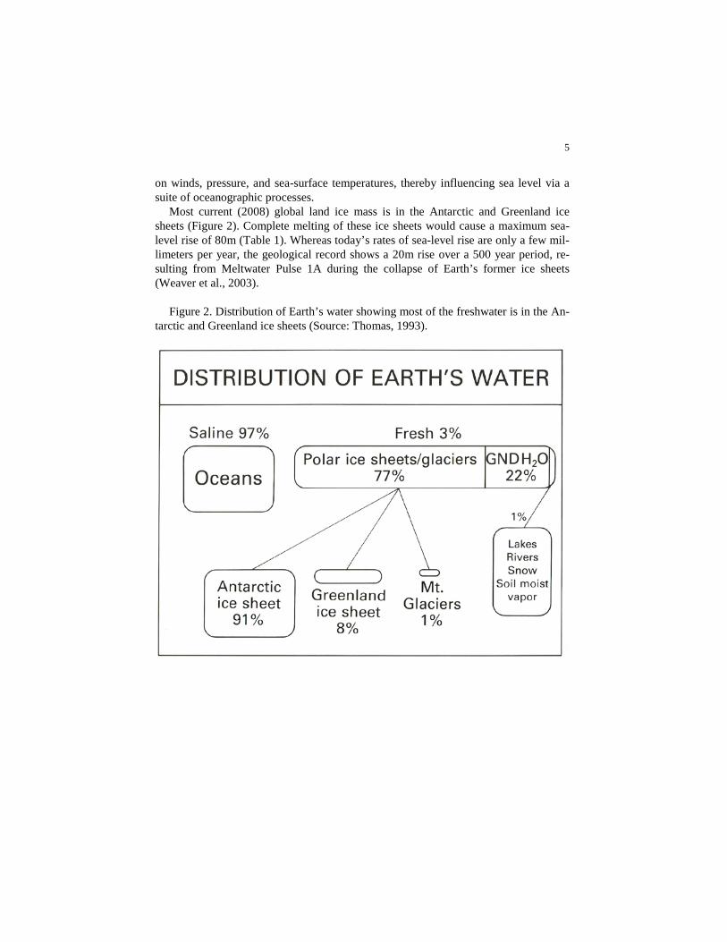
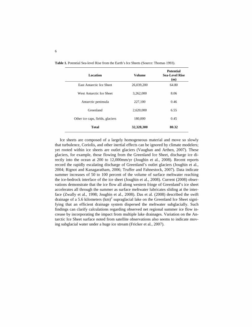
Most current (2008) global land ice mass is in the Antarctic and Greenland ice sheets (Figure 2). Complete melting of these ice sheets would cause a maximum sea-level rise of 80m (Table 1). Whereas today’s rates of sea-level rise are only a few mil-limeters per year, the geological record shows a 20m rise over a 500 year period, re-sulting from Meltwater Pulse 1A during the collapse of Earth’s former ice sheets (Weaver et al., 2003).
Figure 2. Distribution of Earth’s water showing most of the freshwater is in the An-
tarctic and Greenland ice sheets (Source: Thomas, 1993).
6
Table 1. Potential Sea-level Rise from the Earth’s Ice Sheets (Source: Thomas 1993).
Location Volume Potential
Sea-Level Rise (m)
East Antarctic Ice Sheet 26,039,200 64.80
West Antarctic Ice Sheet 3,262,000 8.06
Antarctic peninsula 227,100 0.46
Greenland 2,620,000 6.55
Other ice caps, fields, glaciers 180,000 0.45
Total 32,328,300 80.32
Ice sheets are composed of a largely homogeneous material and move so slowly
that turbulence, Coriolis, and other inertial effects can be ignored by climate modelers; yet rooted within ice sheets are outlet glaciers (Vaughan and Arthen, 2007). These glaciers, for example, those flowing from the Greenland Ice Sheet, discharge ice di-rectly into the ocean at 200 to 12,000mm/yr (Joughin et al., 2008). Recent reports record the rapidly escalating discharge of Greenland’s outlet glaciers (Joughin et al., 2004; Rignot and Kanagaratham, 2006; Truffer and Fahnestock, 2007). Data indicate summer increases of 50 to 100 percent of the volume of surface meltwater reaching the ice-bedrock interface of the ice sheet (Joughin et al., 2008). Current (2008) obser-vations demonstrate that the ice flow all along western fringe of Greenland’s ice sheet accelerates all through the summer as surface meltwater lubricates sliding at the inter-face (Zwally et al., 1998; Joughin et al., 2008). Das et al. (2008) described the swift drainage of a 5.6 kilometers (km)2 supraglacial lake on the Greenland Ice Sheet signi-fying that an efficient drainage system dispersed the meltwater subglacially. Such findings can clarify calculations regarding observed net regional summer ice flow in-crease by incorporating the impact from multiple lake drainages. Variation on the An-tarctic Ice Sheet surface noted from satellite observations also seems to indicate mov-ing subglacial water under a huge ice stream (Fricker et al., 2007).
7
X.3 Storm Surge and Effects: Tsunamis and Hurricanes
Across our planet, civilization is vulnerable to disaster events that can annihilate because they catch individuals by surprise. Sea waves act to dissipate concentrations of energy in the Earth’s dynamic systems that stem from various meteorological or geophysical sources, and can sometimes result in a natural disaster (Zebrowski, 1999). Tsunamis are seismic sea waves generated spontaneously by a rapid release of energy from submarine earthquakes, explosions of sea-level volcanoes, and by undersea landslides along the continental shelves. Tsunamis have long wavelengths and periods, i.e., the time for passage of one wavelength, and the first wave peak hitting land is not necessarily the largest (Zebrowski, 1999). These long periods often cause unexpected wavefronts to hit local populations.
In 2004, a massive tsunami occurred in the Indian Ocean. Coastal areas in Indone-sia, Thailand, India and surrounding locations received significant inundation includ-ing a 30m wave that hit Banda Aceh on the northwestern tip of the island of Sumatra in Indonesia. In Sri Lanka and other locations the wave heights crested 10m or more. Wave heights at these levels can inundate large coastal areas causing significant loss of life and damage to property and infrastructure (as of this writing, a selection of be-fore/after images of the tsunami’s impact on Banda Aceh was available on the World Wide Web at http://homepage.mac.com/demark/tsunami/9.html).
While tsunamis are particularly devastating with high surges of sea water, hurri-canes occur more frequently, in more world locations, and can also cause high water surges. The 1900 Galveston hurricane is on record as the worst natural disaster in US history with an estimated loss of life of between 6000 and 12,000 persons (McGee, 1900; Zebrowski, 1999). Barrier islands, similar to the one on which Galveston is built, are found along the coasts of the US Atlantic Ocean and Gulf of Mexico, and are areas most prone to hammering by high-energy waves and storm surges (Zebrowski, 1999).
On August 28, 2005, Hurricane Katrina passed across the Gulf of Mexico and be-came a Category 5 storm on the Saffir-Simpson hurricane scale, with winds estimated at 175 miles per hour (NOAA, 2007). Hurricane Katrina devastated New Orleans and other Gulf Coast areas destroying lives, homes, and city infrastructure. As of this writ-ing, many people are still coping with Katrina’s devastation. The storm surge was par-ticularly destructive (see http://www.snopes.com/katrina/photos/surge.asp), flooding a large area around New Orleans. Coastal storm surge flooding was 7 to 10m (20 to 30 feet) above normal tide levels (FEMA, 2007). In the same year that Katrina hit the Gulf Coast, Hurricane Rita caused a second wave of devastation a few months later. A series of before and after maps and images of the effects of Katrina and Rita are avail-able from the USGS (2008a).
8
The potential for damage from hurricanes and tsunamis becomes apparent from
these few examples. To better perform risk assessment, understand development op-portunities and challenges, and improve evacuation routing, it is necessary to develop methods to model areas subject to inundation that include the number of persons who could be affected, various land covers (that can impede or exacerbate the movement of coastal surges), and infrastructure at risk. Following is a description of methods em-ployed for global, regional, and local areas.
X.4 Global, Regional, and Local Modeling of Sea-level Rise
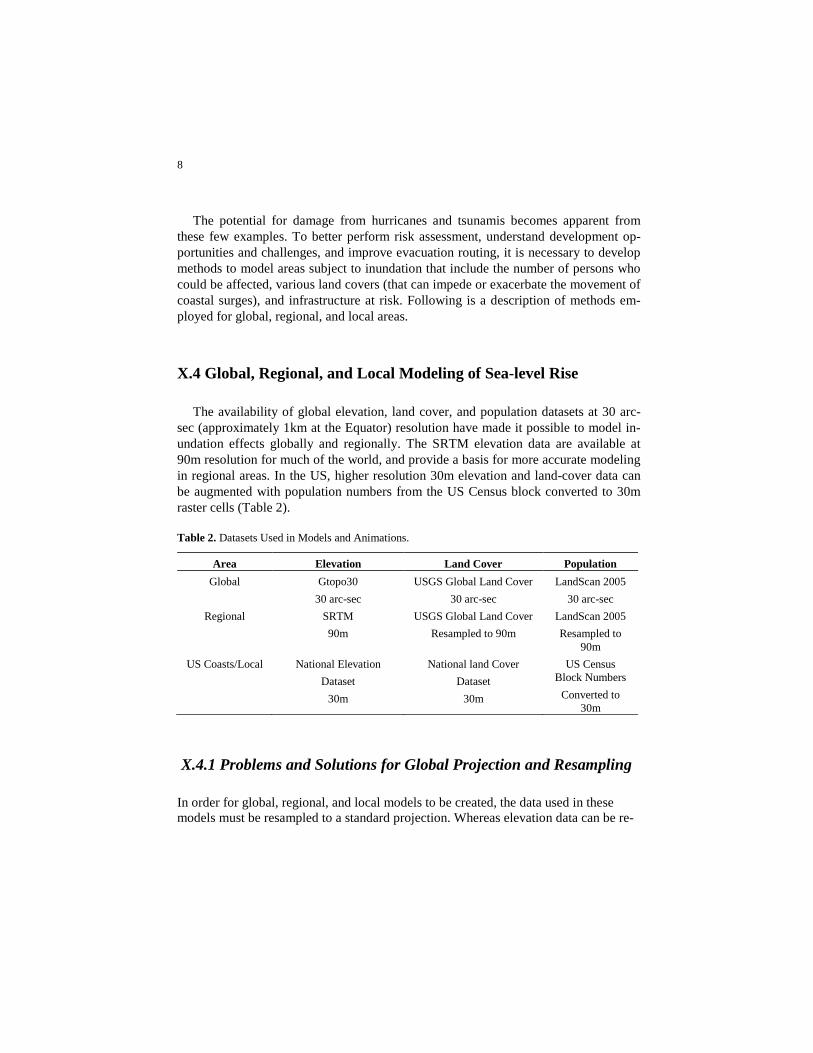
The availability of global elevation, land cover, and population datasets at 30 arc-sec (approximately 1km at the Equator) resolution have made it possible to model in-undation effects globally and regionally. The SRTM elevation data are available at 90m resolution for much of the world, and provide a basis for more accurate modeling in regional areas. In the US, higher resolution 30m elevation and land-cover data can be augmented with population numbers from the US Census block converted to 30m raster cells (Table 2).
Table 2. Datasets Used in Models and Animations.
Area Elevation Land Cover Population Global
Gtopo30
30 arc-sec USGS Global Land Cover
30 arc-sec LandScan 2005
30 arc-sec Regional SRTM
90m USGS Global Land Cover
Resampled to 90m LandScan 2005 Resampled to
90m US Coasts/Local National Elevation
Dataset 30m
National land Cover Dataset
30m
US Census Block Numbers
Converted to 30m
X.4.1 Problems and Solutions for Global Projection and Resampling
In order for global, regional, and local models to be created, the data used in these models must be resampled to a standard projection. Whereas elevation data can be re-
9
sampled with an averaging resampler (e.g., bilinear interpolation), land cover and pop-ulation data require different methods. Categorical (land cover) data must be resam-pled with a nearest neighbor algorithm causing significant pixel gain/loss in some lo-cations (Seong and Usery, 2001; Seong et al. 2002). Population data (numbers of people in each raster cell) cannot be resampled with averaging or nearest neighbor me-thods, but instead require an additive resampler. In the additive resampler, the output pixel value is a result of combination of multiple input pixel values. The software adds all complete input pixels that map to the area covered by a single output pixel. We proportionally assign input pixels that are split across output pixel boundaries. Thus, each output pixel has a unique value (number of people) that results from the additive combination of the appropriate set of input pixels. We validate the process by check-ing the total number of people in the output image against the total number from the input image. These must exactly match so we do not loose or gain people in the re-sampling process.
For global projections, significant problems were encountered with commercial
software when attempting to resample and project the 2 gigabytes (Gb) elevation and 1Gb land cover/population raster files. Software problems included unreliable global projections, inability to account for singularities such as the North and South Poles, and specific projections unable to process to completion (aborting before the plane re-presentation is complete). Inverse projection results moved North America across the Atlantic to the Greenwich meridian, increased file sizes by orders of magnitude, and repeated areas at edges of a global projection (i.e., caused both Alaska and Siberia to appear on both edges of the map). Computation time was also an issue because it can be extensive, lasting up to 200 hours or more on high-end desktop computers (Usery and Seong, 2001; Usery et al. 2003).
To problems such as the above, a USGS software package called mapIMG was used (available from http://carto-research.er.usgs.gov/projection/acc_proj_data.html). To account for pixel loss and gain in categorical data, the resampling method uses a statistical strategy, such as the modal category or some other user-defined strategy. For example, to down-sample the data from a 30 arc-sec to an 8km x 8km pixel, 64 input values are used to determine a single output value. The mapIMG software examines the 64 values and tabulates the number of values in each category. The user can then assign the modal category (the value that occurs the highest number of times) to the output cell. The result is a smoother image of categorical data with a reduction in pixel loss and gain (Steinwand, 2003). For population data, an additive resampler was used. Using the above example of 64 input pixels to one output pixel, the mapIMG software adds the values of the 64 pixels to create one output value. MapIMG, is available for various computing platforms and can be downloaded without charge.
10
X.4.2 Multi-scale Modeling Approach
Global and regional effects of rising sea level are modeled using elevation, popula-tion, and land cover data at 30 arc-sec spatial resolution projected and resampled to 1km cells as described in the previous section. The datasets were transformed to the Mollweide projection to provide a global view with equal areas of land cover (Figure 3), using a decision support system for map projection selection that is freely available to users of global and regional raster/vector datasets (USGS 2008b).
Figure 3. Transformation of the global datasets for elevation, land cover, and popu-lation from geographic coordinates to the Mollweide projection.
The subsequent modeling effort utilizes statistical summaries and animations. Sta-
tistical summaries show sea-level rise effects at global and regional scales, as well as surge effects in low-lying urban areas at local scales and in relation to affected popula-tions and land cover loss. Animations are used to illustrate the locations of affected areas; a blue mask aids the visualization of rising water as it “inundates” existing land cover. One caveat regarding the simulations, animations, and statistical models pre-sented here is that their accuracy is dependent on the resolution and accuracy of the elevation data. Determining the extent of land classes and numbers of people affected
11
depends on the resolution and accuracy of the land cover and population data. As with all models, any errors in these data will be propagated throughout the models, and may invalidate the results.
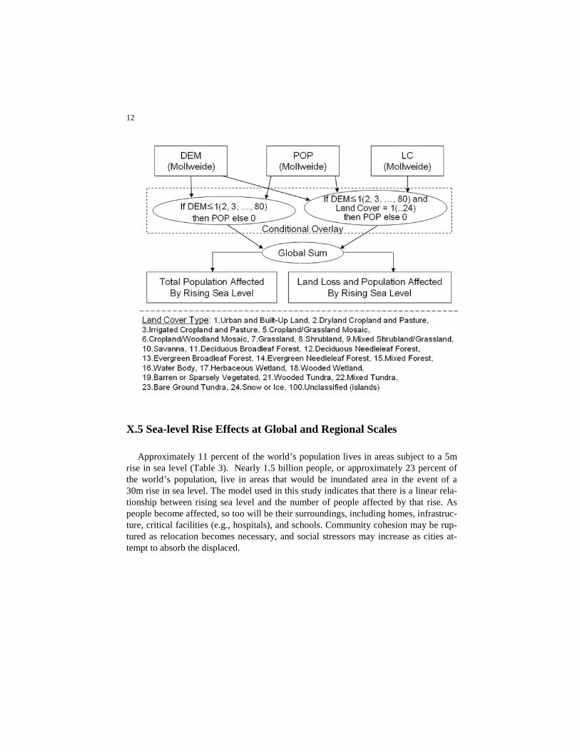
To determine areas of inundation and affected land cover types, and to extract the number of people in inundation areas of specific levels of rise, a conditional overlay and global summation operation are used (Figure 4). The model is established to oper-ate on intervals of sea-level rise and create an output map for each interval. For exam-ple, on a 1m interval, individual maps are created for 1m, 2m, 3m, 4m, 5m and so forth. To extract the number of people residing in the inundation area, the first condi-tional overlay uses population and elevation data. A population value is assigned to an output pixel only when the location is at an elevation equal to, or lower than, the speci-fied elevation in the condition. Otherwise, a 0 value is assigned to the pixel. The second conditional overlay considers both elevation and land cover type from the 25 land cover categories in the Global Land Cover dataset as listed in the figure. If a pixel value is a specified land cover type and meets the elevation condition, the overlay as-signs the population value at the location in the result data. Otherwise, a 0 is also as-signed. The population in the area that is inundated, assigned a blue mask color, is to-taled and shown in the running counter and the land cover categories outside the inundation area are used to set colors for the remainder of the map in the animations.
Figure 4. A schematic of the conditional model used to determine areas of land
cover and numbers of people in areas of inundation.
12
X.5 Sea-level Rise Effects at Global and Regional Scales
Approximately 11 percent of the world’s population lives in areas subject to a 5m rise in sea level (Table 3). Nearly 1.5 billion people, or approximately 23 percent of the world’s population, live in areas that would be inundated area in the event of a 30m rise in sea level. The model used in this study indicates that there is a linear rela-tionship between rising sea level and the number of people affected by that rise. As people become affected, so too will be their surroundings, including homes, infrastruc-ture, critical facilities (e.g., hospitals), and schools. Community cohesion may be rup-tured as relocation becomes necessary, and social stressors may increase as cities at-tempt to absorb the displaced.
Rising sea level impact on people and land cover was examined by exploring the 25 land-cover categories of the Global Land Cover dataset shown in Figure 4. Among these categories, urban and built-up areas contain the highest population densities (about 3600 people per km2); over 960 million people (about 16 percent of the world’s population) live in those areas (Table 4). With a 5m rise in sea level, 125 million people (about 2 percent of world population) living in urban and built-up areas are af-fected, or approximately 13 percent of the total urban population. Other land cover categories with high population densities include three cropland areas, Dry Land Crop-land and Pasture, Irrigated Cropland and Pasture, and Crop Land/Woodland Mosaic, that are residence to more than 50 percent of the world’s population. While population densities are not as high in these areas as in the Urban and Built-up Land, more land falls into this category. Therefore, should sea levels rise 5m in these three cropland areas, over 250 million people would be affected.
Table 4. Population Affected with Major Land Cover Types by Rising Sea Level
* Percentage of total population residing in this land cover type.
X.5.1 Surge Effects at Local and Urban Scales
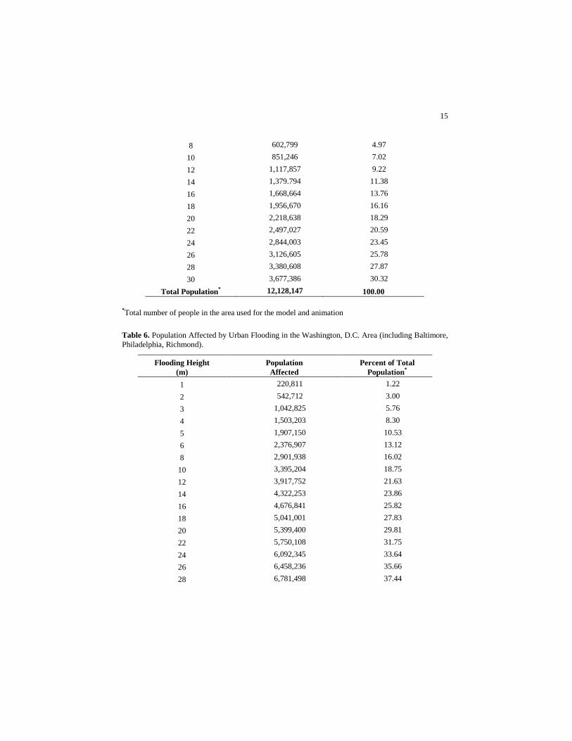
The impacts of 2004’s Indian Ocean Tsunami and 2005’s Hurricanes Katrina and Rita indicate the importance of local flood simulation. From the model, estimates of the number of people affected by 1-30m flooding in the Los Angeles, Washington, D.C., and New York areas are shown in Tables 5, 6, and 7, respectively (note that the numbers reflect the areas selected for modeling and do not apply to urban areas as de-fined by the US Census or other spatially defined boundaries). The highest surge flooding from Hurricane Katrina was 13 feet (approximately 4m) along the coasts of Louisiana and Mississippi. Using 4m as a “design surge” in Los Angeles produces an impact on about 276,000 people; in Washington, D.C. on about 1,500,000; and in the New York area on about 1,300,000. If the flooding is increased to 30m, the approx-imate number of people living in these areas that would be affected is 3,600,000; 7,000,000; and 12,000,000, respectively.
Table 5. Population Affected by Urban Flooding in the Los Angeles Area.
*Total number of people in the area used for the model and animation
X.5.2 Visualization with Animation
Animations can be created using elevation and land cover data by taking “snap-shots” of inundated land cover at particular elevations/water levels. The snapshot im-ages are imported into animation software such as Macromedia® Flash® or Micro-soft® Powerpoint®. The images are arranged sequentially to simulate the rise of sea
17
level from 1-30 m (or, 80m in the case of some of the global and regional animations). Finally, the sequential images are exported to an animation file such as .avi or .wmv to create a flipbook animation.
Figure 5 illustrates land covered by rising sea levels of 5, 10, 20, and 30m in sever-al areas including Florida in the US, the Netherlands in Europe, and China in East Asia. The figure includes the number of people worldwide who would be affected by each level of rise. Most areas in Florida would be flooded by a 30-m rise in sea level. Beijing and Shanghai, the two largest cities in China, would be flooded by 10-20m ris-es. And, in Europe, the western one-half of the Netherlands would be flooded by a 5-m rise in sea level.
Figure 5. Land loss in selected areas and global population affected.
More moderate rises were also modeled to examine localized results. Although the
western coast of the US does not normally experience hurricanes, severe storms can occur in the area, including tropical cyclones and tsunamis (Butler, 2005). Figure 6 displays simulated storm surge flooding in Los Angeles, California. As flood levels increase, the southern part of the city is increasingly flooded. With 30m flooding, about half the city is inundated.
18
Figure 6. Storm surge flooding simulation in the Los Angeles, California area.
Simulations for Washington, D.C. (Figure 7) and New York (Figure 8) show signif-
icantly larger land areas affected by sea level rise. Examining these figures with Tables 6 and 7 demonstrates how low east coast elevations expose more people to in-undation at low levels of rise.
Figure 7. Storm surge flooding simulation in the Washington, D.C. area.
19
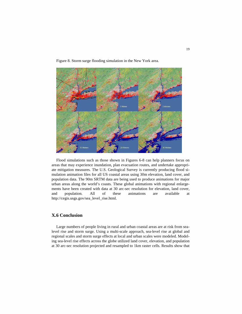
Figure 8. Storm surge flooding simulation in the New York area.
Flood simulations such as those shown in Figures 6-8 can help planners focus on
areas that may experience inundation, plan evacuation routes, and undertake appropri-ate mitigation measures. The U.S. Geological Survey is currently producing flood si-mulation animation files for all US coastal areas using 30m elevation, land cover, and population data. The 90m SRTM data are being used to produce animations for major urban areas along the world’s coasts. These global animations with regional enlarge-ments have been created with data at 30 arc-sec resolution for elevation, land cover, and population. All of these animations are available at http://cegis.usgs.gov/sea_level_rise.html.
X.6 Conclusion
Large numbers of people living in rural and urban coastal areas are at risk from sea-level rise and storm surge. Using a multi-scale approach, sea-level rise at global and regional scales and storm surge effects at local and urban scales were modeled. Model-ing sea-level rise effects across the globe utilized land cover, elevation, and population at 30 arc-sec resolution projected and resampled to 1km raster cells. Results show that
a 5m rise in sea level would potentially affect about 700 million people; of these, 125 million live in urban and built-up areas. A 30m rise places 1.4 billion, or 23 percent, of the world’s people in areas of risk.
Storm surge modeling for Los Angeles, Washington, D.C., and New York is based on 30m resolution data for land cover, elevation, and population. Southern Los An-geles has relatively low elevation so that area is easily flooded. Raising sea level 1m in the Los Angeles area would inundate locations occupied by over 95,000 people; a 1m rise in Washington, D.C. and New York will affect over 220,000 and 240,000 people, respectively. In Los Angeles, a 5m rise would affect over 350,000 people, whereas, in Washington, D.C. and New York, a similar rise inundates over 1,900,000 and 1,800,000 people, respectively. And a 10m rise in global sea level would affect more than 8 million people in these three urban areas.
The methods presented in this chapter are used with available global and regional datasets, limiting the ability to model small sea level change, such as the 3.5mm that is now occurring each year. Higher resolution datasets, such as elevation data from lidar placed on a 10cm grid, can be used to model small rises in sea level using the same methods outlined here. These methods provide a basis for visualizing risk and can help guide urban planning, development and evacuation decisions.
Future research includes the development of complete datasets at 30m resolution for the United States and at 90m for selected parts of the world where large coastal populations are found. An interactive capability allowing users to access these datasets on the World Wide Web to conduct user-selected area of interest simulations is also being developed. Such an interactive capability will permit GIS laymen and the gener-al public to educate themselves and others to the potential harm of global warming through “playing” with the website with different simulations, adjusting areas to those of immediate interest. Additionally, simulations incorporating high resolution lidar da-ta are being created and further refinements are being added, such as data layers con-taining boundaries and place names.
ment of global and regional mean sea level trends from TOPEX and Jason-1 altimetry
21
based on revised reference frame and orbits. Geophysical Research Letters. Volume 34, L14608.
Butler, R. (2005). Hurricane could hit San Diego. Web document. mongabay.com.
http://news.mongabay.com/2005/0908-san_diego.html. Cazenave, A. & Nerem, R.S. (2004). Present-day sea level change: Observations and causes.
Reviews of Geophysics, Volume 42, RG3001. Chambers, D.P. (2006). Observing seasonal steric sea level variations with GRACE and satellite
altimetry, Journal of Geophysical Research, Volume 111, C03010. Chambers, D. (2008). Causes and effects of sea-level rise. Presentation to the National Research
Council Mapping Sciences Committee, April 24, 2008. Chao, B.F., Wu, Y.H., Li, Y.S. (2008). Impact of artificial reservoir water impoundment on
global sea level. Science, Volume 320, 212–214, 11 April. Church, J.A., & Neil J. White (2006). A 20th century acceleration in global sea-level rise. Geo-
physical Research Letters, Volume 33, L01602. Comiso, J.C., Parkinson, C.L., Gersten, R., Stock, L. (2008). Accelerated decline in the Arctic
sea ice cover. Geophysical Research Letters, Volume 35, L01703. Das, S.B., Joughin, I., Hehn, M.D., Howat, I.M., King, M.A., Lizarralde, D., Bhatia, M.P.
(2008). Fracture propagation to the base of the Greenland ice sheet during Supraglacial Lake drainage. Science, Volume 320, 778–781, 9 May.
Demark, T. (2005). Before and after images of areas affected by the Indian Ocean Tsunami,
Web document. http://homepage.mac.com/demark/tsunami/9.html. Douglas, B.C., Kearney, M.S., Leatherman, S.P. (2001). Sea-level rise: History and conse-
quences. New York: Academic Press. FEMA. (2007). About Louisiana Katrina flood recovery maps. Web document. FEMA.
http://fema.gov/hazard/flood/recoverydata/katrina/katrina_la_index.shtm. Fricker, H.A., Scambos, T., Bindschadler, R., Padman, L. (2007). An active subglacial water
system in West Antarctica mapped from space. Science, Volume 315, 1544–1548, 16 Mar. Gehrels, W.R., Hayward, B.W., Newnham, R.M., Southall, K.E. (2008). A 20th century accele-
ration of sea-level rise in New Zealand. Geophysical Research Letters, Volume 35, L02717. Holgate, S.J. (2007). On the decadal rates of sea level change during the twentieth century.
Geophysical Research Letters, Volume 34, L01602.
22
Horton, R., Herweijer, C., Rozenzweig, C., Liu, J., Gormitz, V., Ruane, A.C. (2008). Sea-level rise predictions for current generation CGCMd based on the semi-empirical method. Geo-physical Research Letters, Volume 35, L02715.
Intergovernmental Panel on Climate Change (IPCC). (2007). Climate change 2007: The physi-
cal science basis. In S. Solomon, D. Qin, M. Manning, M. Marquis, K. Averyt, M. Tignor, H.L. Miller, Jr., Z. Chen (Eds.). Cambridge: Cambridge University Press. Internet at http://ipcc-wg1.ucar.edu/wg1/wg1-report.html. Accessed 10 May 2008.
Jenkins, A., & Holland, D. (2007). Melting of floating ice and sea-level rise. Geophysical Re-
search Letters, Volume 34, L16609. Joughin, I., Abdalati, W., Fahnestock, M. (2004). Large fluctuations in speed on Greenland’s
dup along the western flank of the Greenland ice sheet. Science, Volume 320, 781–783, 9 May.
Poore, R.Z., Williams, R.S., Jr., Tracey, C. (2000). Sea level and climate. USGS Fact Sheet
002–00. McGee, W.J. (1900). The lessons of Galveston. National Geographic, October, 377–378. Miller, L., & Douglas, B.C. (2004). Mass and volume contributions to twentieth-century global
sea-level rise. Nature, Volume 428, 406–409, 25 March. NOAA, 2007, Hurricane Katrina—Most destructive hurricane ever to strike the U.S. Web doc-
ument, NOAA. http://www.katrina.noaa.gov. Rignot, E. and Kanagaratnam, P. (2006). Changes in the velocity structure of the Greenland ice
sheet. Science, Volume 311, 986–990, 17 February. Schiefer, E., Menous, B., Wheate, R. (2007). Recent volume loss of British Columbian glaciers,
Canada. Geophysical Research Letters, Volume 34, L16503. Seong, J.C., Mulcahy, K.A., Usery, E.L. 2002. The Sinusoidal Projection: A new meaning for
Global Image Data. The Professional Geographer, Volume 54, no. 2, 218–225. Seong, J.C., & Usery, E.L. 2001. Modeling raster representation accuracy using a scale factor
model. Photogrammetric Engineering and Remote Sensing, Volume. 67, no. 10, p. 1185–1191.
Shepherd, A., & Wingham, D. (2007). Recent sea-level contributions of Antarctic and Green-
land ice sheets. Science, Volume 315, 1529–1532, 16 March.
Steinwand, D., 2003. A new approach to categorical resampling, Proceedings. American Con-gress on Surveying and Mapping Annual Convention, Phoenix, AZ. http://www.acsm.net/sessions03/NewMethodologies41.pdf. Accessed April 2007.
Thomas, R.H., 1993. Ice Sheets. In R.J. Gurney, J.L. Foster, C.L., Parkinson, (Eds.), Atlas of Sa-
tellite Observations Related to Global Change (pp. 385–400). Cambridge, U.K.: Cambridge University Press.
Usery, E.L., & Seong, J.C. (2001). All equal area map projections are created equal, but some
are more equal than others. Cartography and Geographic Information Science, Volume 28, no. 3, 183–193.
Usery, E.L., Finn, M.P., Cox, J.D., Beard, T., Ruhl, S., Bearden, M. (2003). Projecting global
datasets to achieve equal areas. Cartography and Geographic Information Science, Volume 30, no. 1, 69–79.
USGS. (2008a). Products related to Hurricanes Katrina and Rita. Web document. http://store.usgs.gov/mod/HurricaneAreas.html.
USGS. (2008b). Decision support system for map projections of small scale data. U.S. Geolog-
ical Survey. http://mcmcweb.er.usgs.gov/DSS/, Accessed May 2008. Vaughan, D.C., & Arhern, R. (2007). Why is it hard to predict the future of ice sheets? Science,