Modeling soil and landscape evolution – the effect of ...

SOIL, 6, 337–358, 2020https://doi.org/10.5194/soil-6-337-2020© Author(s) 2020. This work is distributed underthe Creative Commons Attribution 4.0 License.

SOIL

Modeling soil and landscape evolution –the effect of rainfall and land-use change

on soil and landscape patterns

W. Marijn van der Meij1,2, Arnaud J. A. M. Temme3,4, Jakob Wallinga1, and Michael Sommer2,5

1Soil Geography and Landscape Group, Wageningen University and Research,P.O. Box 47, 6700 AA, Wageningen, the Netherlands

2Research Area Landscape Functioning, Working Group Landscape Pedology, Leibniz-Centre for AgriculturalLandscape Research ZALF, Eberswalder Straße 84, 15374 Müncheberg, Germany

3Department of Geography, Kansas State University, 920 N17th Street, Manhattan, KS 66506, USA4Institute of Arctic and Alpine Research, University of Colorado, Campus,

P.O. Box 450, Boulder, CO 80309-0450, USA5Institute of Environmental Science & Geography, University of Potsdam,

Karl-Liebknecht-Straße 24–25, 14476 Potsdam, Germany

Correspondence: W. Marijn van der Meij ([email protected])

Received: 24 October 2019 – Discussion started: 7 November 2019Revised: 12 May 2020 – Accepted: 2 June 2020 – Published: 3 August 2020

Abstract. Humans have substantially altered soil and landscape patterns and properties due to agricultural use,with severe impacts on biodiversity, carbon sequestration and food security. These impacts are difficult to quan-tify, because we lack data on long-term changes in soils in natural and agricultural settings and available sim-ulation methods are not suitable for reliably predicting future development of soils under projected changes inclimate and land management. To help overcome these challenges, we developed the HydroLorica soil–landscapeevolution model that simulates soil development by explicitly modeling the spatial water balance as a driver ofsoil- and landscape-forming processes. We simulated 14 500 years of soil formation under natural conditions forthree scenarios of different rainfall inputs. For each scenario we added a 500-year period of intensive agriculturalland use, where we introduced tillage erosion and changed vegetation type.

Our results show substantial differences between natural soil patterns under different rainfall input. Withhigher rainfall, soil patterns become more heterogeneous due to increased tree throw and water erosion. Agri-cultural patterns differ substantially from the natural patterns, with higher variation of soil properties over largerdistances and larger correlations with terrain position. In the natural system, rainfall is the dominant factor influ-encing soil variation, while for agricultural soil patterns landform explains most of the variation simulated. Thecultivation of soils thus changed the dominant factors and processes influencing soil formation and thereby alsoincreased predictability of soil patterns. Our study highlights the potential of soil–landscape evolution modelingfor simulating past and future developments of soil and landscape patterns. Our results confirm that humans havebecome the dominant soil-forming factor in agricultural landscapes.

Published by Copernicus Publications on behalf of the European Geosciences Union.

338 W. M. van der Meij et al.: Modeling soil and landscape evolution

1 Introduction

Soils provide valuable functions for nature and society bysupporting plant growth and agriculture, managing water andsolute flow, sequestering carbon, preserving archaeologicalheritage, creating habitats for plants and animals and provid-ing support for infrastructure (Dominati et al., 2010; Greineret al., 2017). However, soils are currently degrading by agri-cultural intensification and climate change, forming one ofthe largest threats to global food security and biodiversity(Bai et al., 2008; Montanarella et al., 2016; Tscharntke et al.,2012). A drastic change in land management is needed to re-store healthy soils and soil functions (IPCC, 2019). Combat-ing soil degradation and promoting sustainable land manage-ment therefore stands high on the agenda of the soil sciencecommunity (Bouma, 2014; Cowie et al., 2018; Keesstra etal., 2018; Kust et al., 2017; Minasny et al., 2017).

The first step towards sustainable land management and areturn to healthy, natural soils is a fundamental understand-ing of the development and characteristics of natural soil pat-terns and how these change under human influence. There-fore, we will focus in this paper on gently to strongly slop-ing undulating landscapes that are suitable for agriculturaluse (maximum slope ∼ 20 %, Bibby and Mackney, 1969).Soil-forming processes are controlled by at least five envi-ronmental factors: climate, organisms, relief, parent materialand time (the ClORPT model, Jenny, 1941). Different fac-tors dominate in natural and agricultural settings. In naturalsettings with flat or undulating topography, soil erosion gen-erally occurs at very low rates or is absent (Alewell et al.,2015; Wilkinson, 2005). Some soil redistribution can occuras a consequence of creep or tree throw (Gabet et al., 2003).More importantly, tree throw creates local pits and mounds,which temporarily change hillslope hydrology and act as lo-cal hotspots for soil development due to a larger influx of wa-ter (Šamonil et al., 2015; Shouse and Phillips, 2016). Theseseemingly random processes create a high degree of hetero-geneity in soil patterns, which shows little to no correlationwith relief (Vanwalleghem et al., 2010). In contrast, inten-sively managed agricultural landscapes show soil patternsthat closely follow the relief (Phillips et al., 1999; Van derMeij et al., 2017). This reflects the fact that erosion pro-cesses are relief-dependent, and this propagates into the soilpatterns, unless erosion and deposition patterns are affectedby field margins such as hedges or banks. The switch fromsuch natural to agricultural soil systems can occur abruptly,e.g., by deforestation or the implementation of highly mech-anized agriculture in a few decades. Sommer et al. (2008)described this switch in boundary conditions and its implica-tions with a time-split approach: over a short time period –relative to Holocene soil evolution – the soil system changesfrom natural, progressive pedogenesis, where profile deep-ening and horizon formation dominate erosive processes, toregressive pedogenesis, where – vice versa – erosion and de-

position dominate progressive pedogenic processes (Johnsonand Watson-Stegner, 1987).

The coexistence of both progressive and regressive pro-cesses in a defined period of time has been described by sev-eral authors. In a progressive phase there are also regressiveprocesses that change soils, terrain and hydrological path-ways (Phillips et al., 2017; Šamonil et al., 2018). In a re-gressive phase, progressive processes still have a substantialeffect on soil development (Doetterl et al., 2016; Montagneet al., 2008). Colluvic soils might be influenced by ground-water or subject to continuous clay illuviation (Leopold andVölkel, 2007; Van der Meij et al., 2019; Zádorová and Penížek, 2018). Furthermore, the changes in boundary conditionsare not always as abrupt as, e.g., deforestation. Historic ero-sion processes with rates much lower than current erosionprocesses might have given pedogenic processes the time toalter soil and colluvium (Van der Meij et al., 2019).

To disentangle complex history and causes of soil forma-tion, data are required on both natural and agricultural soilsthat have formed under similar conditions, and preferablyfrom the same region. However, there is limited undisturbednatural land left, often rapidly declining, in places that areunsuitable for agriculture and/or indirectly influenced by an-thropogenic climate change (e.g., tropical and boreal zones,IPCC, 2019). Moreover, (historical) cultivation occurred inareas and soils most suitable for agriculture (Pongratz et al.,2008; Vanwalleghem et al., 2017), leaving less suitable landundisturbed. This complicates comparison and empirical in-ference. Because of the complex interactions between pedo-genic and geomorphic processes, and the lack of field data,we heavily depend on process knowledge and model simu-lations for mechanistic inference about how natural soil pat-terns develop as a function of their environments and howthis changes in agricultural settings (Opolot et al., 2015).

Soil evolution models simulate a range of physical, chem-ical and biotic processes that affect the properties of soilsthrough space and time (Minasny et al., 2015; Stockmann etal., 2018; Vereecken et al., 2016). Such models have beendeveloped for a range of scales, varying from 1D soil pro-files to 3D soil landscapes (Finke, 2012; Minasny et al.,2015; Temme and Vanwalleghem, 2016). One-dimensionalsoil profile models generally provide a high level of detailand process coverage, but they lack the simulation of essen-tial feedbacks and interactions that can occur between soilson a landscape scale (Van der Meij et al., 2018). For example,the spatial redistribution of water or the exchange of soil ma-terial through erosion and deposition processes affects soilsdifferently at different landscape positions. Soil landscapeevolution models (SLEMs) do simulate lateral distributionof solids by geomorphic processes and consider soils to becontinua rather than discrete units. Current SLEMs performreasonably well in landscapes where lateral soil movementis substantial (e.g., Temme and Vanwalleghem, 2016; VanOost et al., 2005). However, these models are not developedto simulate soil development in relatively stable landscapes

SOIL, 6, 337–358, 2020 https://doi.org/10.5194/soil-6-337-2020

W. M. van der Meij et al.: Modeling soil and landscape evolution 339

where lateral water redistribution is the dominant driver caus-ing soil heterogeneity, because this hydrologic control is notexplicitly modeled (Van der Meij et al., 2018).

To summarize, we are currently lacking data and methodsthat can quantify the effect of changing soil-forming factorson soil development and spatiotemporal soil patterns. Thisknowledge is essential for the transition to sustainable landmanagement and adaptation to the changing climate. The ob-jective of this study is to develop a suitable model for quan-tifying the variation and predictability of soil patterns as afunction of varying environmental factors. We will addressthree questions.

1. What are the basic characteristics of soil patterns in nat-ural and agricultural landscapes?

2. What are the major factors driving soil formation in nat-ural and agricultural landscapes?

3. How does the predictability of soil patterns changethrough time and after cultivation?

We developed a soil–landscape evolution model that cansimulate natural soil and landscape evolution by incorporat-ing dominant natural processes such as soil creep, tree throw,vegetation dynamics and infiltration-dependent pedogenesisdriven by the soil-forming factors climate, organisms, relief,parent material and time. We simulated soil formation for14 500 years under three scenarios of rainfall (dry, humid,wet) to quantify the effect of water availability and distri-bution on soil variation in natural systems. Each run wasconcluded with 500 years of intensive agricultural land use,where we introduced the process of tillage erosion. Tillageerosion is a dominant process redistributing soil materialin intensively managed agricultural fields (Van Oost et al.,2005).

We expect that before intensive cultivation, spatial soil het-erogeneity will be larger for greater rainfall, due to more in-tense erosion and translocation processes and effects of veg-etation. Moreover, we expect that the spatial heterogeneitywill increase by erosion processes under cultivation, also re-sulting in larger correlations between soil properties and to-pographic properties, because of the topographic dependenceof erosion processes. This would imply that soil patterns be-come more predictable due to cultivation, at least for circum-stances without hedges or banks that would modify the spa-tial distribution of erosion and deposition areas.

For our simulations, we created a hypothetical loess-covered, hilly landscape with a range of characteristic slopepositions as the spatial setting. We choose loess, because itis a relatively homogeneous parent material, widely spreadglobally and favored for agricultural practices due to its highwater-holding capacity and resulting fertility (Catt, 2001).The long-term use of loess areas for agriculture and unsus-tainable management has resulted in severe land degradation(e.g., Zhao et al., 2013).

2 Methods

2.1 Model

Here we describe our model named HydroLorica. HydroLor-ica is based on the model Lorica (Temme and Vanwalleghem,2016), but includes explicit simulation of water flow andwater availability as drivers of natural soil, landscape andvegetation change (Van der Meij et al., 2018). HydroLoricais a reduced-complexity model, which means that it simu-lates processes affecting soil and landscapes using simpli-fied process descriptions. Reducing model complexity pro-motes critical evaluation of essential processes, reduces cal-culation time and prevents extensive data requirements andover-parameterization (Hunter et al., 2007; Kirkby, 2018;Marschmann et al., 2019; Snowden et al., 2017; Temme etal., 2011).

2.1.1 Model architecture

HydroLorica is a raster-based model, where a digital ele-vation model (DEM) determines the shape of the terrain.Below each raster cell of the DEM there is a predeter-mined number of soil layers with layer thicknesses variablein space and time. Each layer can contain a specific mix-ture of gravel, sand, silt and clay and two types of organicmatter (quickly and slowly decomposing, Yoo et al., 2006),depending on parent material and occurring pedogenic pro-cesses. Pedogenic and geomorphic processes affect the con-tents of the layers, leading to differences in soils in spaceand time. Changes in soil properties and contents modifylayer thicknesses and surface elevation through a pedotrans-fer function (PTF) of bulk density. The use of a pedotransferfunction allowed the model to calculate variations in layerthicknesses due to pedogenic and geomorphic processes. Weused the same PTF for bulk density as the original Loricamodel (Tranter et al., 2007). We refer to Temme and Vanwal-leghem (2016) for more information about the spatial modelarchitecture of Lorica, which we maintained in our adapta-tion HydroLorica. In this project, we worked with 25 soillayers, with an initial uniform thickness of 0.15 m. When alayer got very thick or very thin (55 % thicker or thinner thanits initial value), the layer was split or combined with anotherlayer.

The annual changes in texture classes tex (kg) and organicmatter classes om (kg) in layer l at location xy and time t

are governed following Eqs. (1) and (2) (for abbreviationsof processes, see Table 1). The changes in mass of textureand organic matter are converted to a change in layer thick-ness (m) using a pedotransfer function (Tranter et al., 2007).We calculated the bulk density of the fine mineral fraction(kg m−3) with Eq. (3) using the sand and silt fraction (–) andthe depth below the surface (m). HydroLorica includes a cor-rection of bulk density taking into account the effects of thecoarse fraction and the organic fraction using Eq. (4), using

https://doi.org/10.5194/soil-6-337-2020 SOIL, 6, 337–358, 2020


a density of 2700 kg m−3 for the coarse fraction (Temme andVanwalleghem, 2016) and a density of 224 kg m−3 for theorganic fraction (Tranter et al., 2007). In our study, there isno coarse soil material present. This pedotransfer functiondoes not directly take into account changes in bulk densitystemming from soil structuring, weathering or bioturbation.Instead, depth below the surface is used as a proxy for thesefactors. The used PTF has a relatively low fit with the data itwas derived from (R2

= 0.41, Tranter et al., 2007). However,PTFs that yield a higher accuracy often require advanced cal-culation methods (Chen et al., 2018; Ramcharan et al., 2017)or soil properties that are not readily available in HydroLor-ica. As we discuss in Van der Meij et al. (2018), the estima-tion of such properties often gives biased or highly uncertainresults, which would propagate into the calculation of bulkdensity. Rather than stacking pedotransfer functions, we de-cided to use a PTF that required input that is readily availablein HydroLorica and could be calculated within the model it-self.

The sum of changes in layer thickness of all layers L cal-culated through changes in bulk density and mass of the lay-ers results in the annual change in elevation z (Eq. 5). Claytranslocation and water erosion are directly driven by the to-tal annual water flow, while occurrence of tree throw andrates of creep, bioturbation and organic matter accumulationare indirectly driven by water availability via vegetation con-trols. Infiltration I is the difference between precipitation P

and spatially explicit actual evapotranspiration ETa, runonROnn and runoff ROff (Eq. 6). HydroLorica works with dy-namic time steps as suggested by Van der Meij et al. (2018) tocapture process dynamics at their relevant scales while opti-mizing calculation time. Hydrologic processes are calculatedwith a daily, monthly, or yearly time step, with smaller timesteps selected during wetter conditions for more accuratesimulation. Annual sums of infiltration and overland flow areused to drive geomorphic, pedogenic and biotic processes.

1texxy,l,t =1texCR,xy,l,t +1texWE,xy,l,t

+1texTT,xy,l,t +1texTI,xy,l,t

+1texCT,xy,l,t +1texBT,xy,l,t (1)

1omxy,l,t =1omCR,xy,l,t +1omWE,xy,l,t

+1omTT,xy,l,t +1omTI,xy,l,t

+1omCAB,xy,l,t +1omBT,xy,l,t (2)

BDfine,xy,l,t = 1000(1.35+ 0.452(fsand+ 0.76fsilt)

+ (100(fsand+ 0.76fsilt)− 44.65)2

×− 0.000614+ 0.06 · log10 (depth))

(3)

BDsoil,xy,l,t =masstotal,xy,l,t

massfine,xy,l,t

BDfine,xy,l,t+

masscoarse,xy,l,t

2700 +massorganic,xy,l,t

224

(4)

1zxy,t =

∑L

l=11BDsoil

(∑texxy,l,t +

∑omxy,l,t

)(5)

Table1.O

verviewof

processessim

ulatedin

HydroL

orica,includingdriving

soil-forming

factorsin

them

odelandlandscape

variablesthatare

affectedby

eachprocess.H

umans

areconsidered

anadditionalsoil-form

ingfactor(A

mundson

andJenny,1991;R

ichteretal.,2015).

Soil-forming

factorL

andscapevariable

affected

ProcessA

bbreviationC

limate

Organism

sR

eliefParent

Hum

ansTopography

SoilW

aterV

egetation(rainfall)

(vegetationm

aterialproperties

balancetype

type)(soiltexture)

Bioturbation

BT

XX

Carbon

accumulation

andbreakdow

nC

AB

XX

Clay

translocationC

TX

XX

Creep

CR

XX

XX

Pedon-scalew

aterpartitioningW

PX

XX

XSurface

flowSF

XX

XX

TillageT

IX

XX

XTree

throwT

TX

XX

XV

egetationselection

VS

XX

XX

XW

atererosionW

EX

XX

XX

X



Ixy,t = Pt −ETaxy,t +ROnnxy,t −ROffxy,t (6)

2.1.2 Process formulation and parameters

In our model we considered only the impact of physical andbiological processes on soil properties. The current modelarchitecture does not facilitate the simulation of soil chem-ical processes. The selected processes are described below.Drivers and impacts of each process are summarized in Ta-ble 1. We summarized the drivers per soil-forming factor. Wemostly used the processes and parameters of Lorica as re-ported in Temme and Vanwalleghem (2016), which we sum-marize here. When we added a new process or changed itsparameters, the adjustments are reported in this section. Weprovided a detailed overview of the equations and selectedparameters in Supplement 1.

We aim to understand the functioning of general soil–landscape systems. Therefore, we parametrized and cali-brated the model processes using regional data or processrates from the literature that are valid for larger regions. Wedid not calibrate the parameters on data from one specificstudy site to avoid the effect of any idiosyncrasies that can bepresent in those data. For other processes where there wereno regional data available, we estimated the parameters sothat the effects of those processes were on the same order ofmagnitude as processes with rates based on the literature. Anoverview of the process parameters is provided in Table S1in the Supplement.

Hydrologic processes

The hydrological module partitions spatially uniform rain-fall (P ) into three spatially explicit components: evapotran-spiration (ET), infiltration (I ) and surface flow (ROnn andROff, Eq. 6). Potential ET is calculated from prescribed tem-perature using the Hargreaves–Samani equation (Hargreavesand Samani, 1985) and corrected for topographical position(Swift, 1976) and vegetation type (Allen et al., 1998). Sur-face flow is calculated on a daily basis, and only when rainfallintensity (amount / duration, mm h−1) exceeds the saturatedhydraulic conductivity of the topsoil, which is a function ofsoil properties and slope (Morbidelli et al., 2018; Wösten etal., 2001), or precipitation in the form of snow is melting.The excess water is routed over the surface using the multi-ple flow algorithm (Holmgren, 1994) and can re-infiltrate inplaces with higher hydraulic conductivity, in local surface de-pressions, or can leave the catchment. HydroLorica can thusdeal with DEMs that contain depressions and actively formsdepression by simulating tree throw. The annual sum of dailysurface flow is used to calculate annual water erosion and de-position using the stream power law. To account for seasonaldifferences, actual ET is calculated on a monthly basis fromthe potential ET and rainfall using the topsoil water budgetmodel of Pistocchi et al. (2008). Infiltration is the sum of (re-)infiltrated surface water and the monthly difference between

rainfall and actual ET (Eq. 6). The annual water balance isused as a driver of various geomorphic and pedogenic pro-cesses and to determine vegetation type. The hydrologicalmodule is described in detail in Appendix A of Van der Meijet al. (2018).

Determination of vegetation type

We considered two types of natural vegetation: grassland andforest. The vegetation type depends on the water availabil-ity; where rainfall plus re-infiltration exceeds potential evap-otranspiration, there is no water stress and forests can grow.Otherwise, there is water stress and there will be grassland.This threshold is based on a hypothesis from Thompson etal. (2010), who used the Budyko curve (Budyko and Miller,1974) to estimate vegetation type. By extending this relation-ship with re-infiltration, this relation can be used to assess lo-cal but spatially explicit vegetation type. Vegetation type thushas a climatic control and a topographic control in the formof hillslope aspect and local convergence of water flow ingullies and depressions (e.g., Metzen et al., 2019). This vari-ation in moisture and vegetation can occur very locally, espe-cially in semi-arid regions. Vegetation type influences evapo-transpiration (Allen et al., 1998), bioturbation and creep rate(Gabet et al., 2003) and the occurrence of tree throw, andalso controls organic matter input. Under intensive agricul-tural use, we convert the vegetation type to arable crops. Weassume that soil and landscape processes are similar to land-scapes under grassland vegetation. The differences are thatarable crops have lower potential evapotranspiration and theprocess of tillage is introduced.

Our method of estimating vegetation type can lead to an-nual changes in vegetation type depending on water avail-ability, because we do not consider ecological processes suchas resilience or succession. The portion of years with grass-land and forest vegetation aggregated over longer time spans(>100 yr) provides an estimate for the forest cover of thatspecific location (see the animations in Supplement 2). Thevegetation distribution should thus be considered on an ag-gregated level rather than an annual level to yield meaningfulresults. This implementation suffices for our focus on long-term changes in soils and terrain, but should not be used tostudy systems on annual to decadal timescales.

(Bio-)geomorphic processes

The main (bio-)geomorphic processes affecting topographyin loess areas are soil creep, tree throw, water erosion andtillage erosion. Soil creep is a bio-geomorphic process thatcauses a diffuse movement of soil material on a hillslope,driven by various factors such as (micro)climate, organismsand terrain (Pawlik and Šamonil, 2018; Regmi et al., 2019;Roering et al., 2002). The potential creep rate is a functionof vegetation type and slope (Gabet et al., 2003). We adopthigher creep rates in forested areas, because of the deeper



rooting depth and higher root abundance. We divided the po-tential creep rate at a certain location over all soil layers,with exponentially decreasing rates deeper in the soil. Thetransport of soil material from a layer to layers in its lower-lying neighboring cells is proportional to the surface slopeand shared layer boundaries.

Tree throw is a bio-geomorphic process that has a distincteffect on the terrain and water routing; the created pit can actas a hotspot for soil formation by the increased infiltration ofwater (Šamonil et al., 2018). We simulated tree throw as arandom process, with on average 0.2 trees falling per hectareper year. This rate is lower than other rates found in natu-ral forests around the world (0.3–1.5 trees ha−1 yr−1, Finkeet al., 2013; Gallaway et al., 2009; Phillips et al., 2017), be-cause some factors controlling tree uprooting like shallowrooting depths due to impermeable layers or steep slopes arenot present in our spatial setting. The dimensions of the rootclump that is transported by tree throw were scaled with theage of the falling tree, which was also randomly selected.We assumed that tree growth occurs in the first 150 yearsof a tree’s existence, after which size remains stable until amaximum age of 300 years. These numbers and trends areloosely based on Rozas (2003). A pit and mound topographyis only formed when the dimensions of the root clump ex-ceed the size of the raster cell (1.5 m in our case) and thatmaterial is transported to a cell downslope. When the rootclump is smaller than the cell size or when the slope of theterrain does not lead to downward transport of the material,tree throw will only cause a (partial) turbation of the upperlayers in the affected raster cells.

Water erosion and deposition are calculated using thesame approach as the original Lorica model (Temme andVanwalleghem, 2016). Sediment uptake and deposition arecalculated as a function of discharge and surface gradients(Schoorl et al., 2002). Sediment uptake is simulated as a se-lective process, where smaller particles are easier to erodeand more difficult to deposit. Organic matter behaves thesame as clay under erosion, because we assumed that or-ganic matter occurs in associations with clay particles. Watererosion is limited by the occurrence of coarse soil particles(surface armoring) and vegetation. The role of water erosionin forested loess catchments is limited (Vanwalleghem et al.,2010); the vegetation protects the soil below from erosion.However, disturbances such as forest fires can temporarilyincrease erodibility of the soil. Therefore, we did simulatewater erosion in forested landscapes, but with lower ratesthan in grassland. We simulated this by including a high veg-etation protection constant (value of 1) in forested sites. Ingrasslands we used the aridity index between 0 and 1 as thevegetation protection constant.

Tillage erosion was simulated as a diffusive process, simi-lar to creep, with some differences: tillage homogenized thesoil over the reach of the plough depth, erosion only occurredfrom the top layer contrary to the whole soil profile as with

creep, and the erosion rates were much higher due to the in-tensive land management.

(Bio-)pedogenic processes

We simulated three dominant (bio-)pedogenic processes thatchange texture and organic matter properties in loess land-scapes. These are clay translocation, bioturbation and soilorganic matter accumulation and breakdown.

We adapted a new way of simulating clay translocation,using the advection equation of Jagercikova et al. (2017).The diffusive part of clay translocation as described by Jager-cikova et al. (2017) is separately modeled by bioturbation.We scaled the parameters of clay translocation with local in-filtration to develop an infiltration-dependent equation. Notall clay in the soil is available for translocation. Part of it isnot available to the percolating water, because it is bondedto other minerals and organic matter. We used the equationsof Brubaker et al. (1992) to estimate the part of the claythat is water-dispersible, i.e., that is available for translo-cation by water. We estimated the required cation exchangecapacity (CEC) with a pedotransfer function from Ellis andFoth (1996), as a function of clay content and organic mattercontent. Following from these equations, the fraction of non-dispersible (remaining) clay is 5.9 % in soils without soil or-ganic matter (SOM) and increases with 1.2 % for every extrapercent of SOM. This approach is similar to the one used insoil profile model SoilGen2 (Finke, 2012).

Bioturbation works as a diffusive processes, homogeniz-ing the soil vertically (Yoo et al., 2011). We used the samerates for bioturbation as for creep, because these processesare driven by the same organisms reworking the soil. Thepotential bioturbation rate was divided over each soil layerby integrating the exponential depth function over the layerthickness and then dividing by the integration of the functionover the entire soil profile. Every layer exchanges a certainfraction of its contents, based on initial bioturbation rate anddepth, with all other layers. The amount of exchange betweentwo layers decreases with increasing distance.

SOM accumulation and breakdown were simulated asin earlier soil–landscape evolution models (Minasny et al.,2008; Temme and Vanwalleghem, 2016; Vanwalleghem etal., 2013; Yoo et al., 2006). Accumulation of SOM is con-trolled by the potential input and depth in the soil. The ac-cumulation is divided over a young and old SOM pool us-ing a fractionation factor. These pools differ in their rate ofdecomposition. We calibrated the SOM cycle in agriculturalsettings with the average depth distribution of organic car-bon in agricultural soils on the Chinese loess plateaus (Liu etal., 2011). We simulated 5000 years of soil development us-ing different process parameters. We selected the parameterset that simulated an organic matter distribution most simi-lar to the reference distributions from Liu et al. (2011). Thereported depth distributions for pasture and forest soils byLiu et al. (2011) were not useful for this project. Soils under



these vegetation types on the Chinese loess plateau generallycontain lower SOM stocks than natural landscapes, becausethese positions often have recently been replanted to combatsoil erosion or because they occur in topographic positionswhich are not favorable for plant growth and agriculture. In-stead, we calculated reference carbon stocks for forest andgrassland soils by adjusting the agricultural carbon stocks ofLiu et al. (2011) with changes in carbon stocks after conver-sion from forest to crop and from forest to pasture (Guo andGifford, 2002). With the resulting reference carbon stocks fornatural vegetation we ran additional calibrations to calculatethe potential SOM input for forest and grassland.

2.2 Experimental setup

We developed an artificial topographic setting in which weperformed our simulations. The use of an artificial settingrather than a field setting avoids the effect of local distur-bances and idiosyncrasies which can disturb general signalswe look for in the model results.

The input DEM is an artificially created U -shaped val-ley of 150 by 150 m, with a cell size of 1.5 m (Fig. 1). Theslopes facing northward and southward have a sinusoid form,and valley depth increases eastward, from 0 to 9 m. Randomnoise of maximum 1 cm was added. The maximum slopeis 12◦ (21 %), which reaches the limit for agricultural use(Bibby and Mackney, 1969). The small cell size of 1.5 mis required to simulate the effect of pit and mound topog-raphy created by tree throw on spatial infiltration patterns.The landscape was designed to display typical topographicfeatures present in loess areas, but we exaggerated the spa-tial variation of slope positions to limit catchment size andreduce calculation time.

As parent material we chose a homogeneous loess withoutcarbonates and a soil texture of 15 % sand, 75 % silt and 10 %clay, which falls in the typical range of loess deposits (Muhs,2007; Pécsi, 1990). We assumed an infinite loess thickness toavoid any effects of layers underneath with different litholo-gies. However, for computational reasons, we worked withan initial loess layer of 3 m with free leaching of water anddispersed clay at the lower boundary. This approach reducedthe number of soil layers and prevented numerical instabil-ity from the pedotransfer function for depth-dependent bulkdensity. The selected thickness left sufficient soil material sothat the bottom of the loess was not reached by erosion dur-ing any of the model runs.

The model requires a latitude to calculate solar inclina-tion on the slopes. We selected the latitude of 50◦ N, whichis in the center of the range for loess occurrence reportedby Muhs (2007, 40–60◦ N). We selected the rainfall scenar-ios based on most common rainfall in loess areas. For this,we made an overlay of a coarse-resolution global loess map(Dürr et al., 2005) with a global annual rainfall map (Fick andHijmans, 2017). The distribution of rainfall from the overlayshowed peaks at ∼ 600 and ∼ 900 mm (Fig. 1). We selected

these annual quantities of rainfall as input for our scenar-ios and we added a scenario of 300 mm to capture a widerrange of climates. The model requires as input daily data onrainfall (m), rainfall duration (h), and minimum, mean andmaximum temperature (◦C). Rainfall amount is required tocalculate how much water flows through the soil landscape.Rainfall intensity is required to determine whether and howmuch overland flow occurs, by comparing rainfall intensitywith soil hydraulic conductivity. Rainfall intensity is calcu-lated by dividing the rainfall amount by the daily duration(m h−1). Temperature data are required to calculate poten-tial evapotranspiration (Hargreaves and Samani, 1985). Aswe want to simulate general trends in soil and landscape evo-lution, we do not need site-specific data for the different sce-narios. Instead, an arbitrary weather dataset was scaled tothe total amount of rainfall from the different climate sce-narios. We used weather data from German weather stationGrünow, which is located at 53.3◦ N, 13.9◦ E (DWD ClimateData Center (CDC), 2018a, b). The potential evapotranspi-ration is around 600 mm yr−1 for this dataset and is appliedto all simulations. Combined with the rainfall scenarios, thescenarios can roughly be classified as dry (300 mm rainfall),humid (600 mm rainfall) and wet (900 mm rainfall). In therest of this paper, we will use the terms dry, humid and wetto refer to the different rainfall scenarios.

We simulated the development of soils and landscapes for15 000 years, resembling the age of most post-glacial soils.In the first 14 500 years of the simulations, soil and land-scape development occurred under natural conditions andland cover. In the last 500 years of the simulations, we intro-duced agricultural land use by changing vegetation type andintroducing tillage erosion. This duration was selected be-cause it loosely reflects the onset of Medieval intense agricul-ture in many areas (Van der Meij et al., 2019) and should beseen as an upper limit of the onset of intensive tillage. Eachof our simulations assumes a constant climate throughout the15 000 simulated years. Although we expect our model to besuitable for investigating the effects of a changing climate onsoil and landscape evolution, this is beyond the scope of thisstudy.

2.3 Analysis and evaluation

The model potentially outputs all soil properties for eachlayer at each location at each time step. Additionally, ele-vation change resulting from all processes at each location ateach time step can be saved. In order to be able to interpretthe results, we had to aggregate the results in several ways.We focused on select soil and terrain properties. The selectedsoil properties are soil organic matter stock (kg m−2), whichis the total amount of SOM in a soil column, and the depthto the Bt horizon (m), which we defined as the depth wherethe clay content first exceeds the initial clay fraction of thesoil. The selected terrain properties are slope (◦), topographicposition index (TPI; m), calculated with square windows



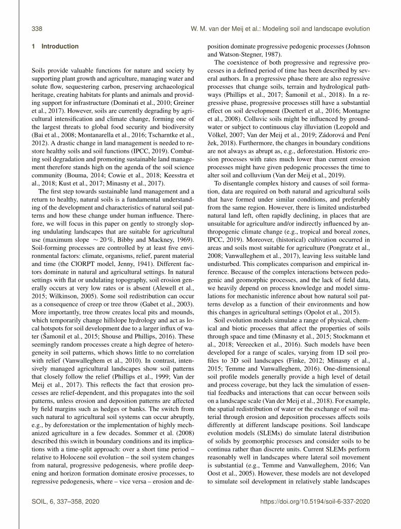
Figure 1. (a) Annual rainfall in loess areas, derived from WorldClim. Red lines indicate the rainfall scenarios in this study: 300 (dry), 600(humid) and 900 (wet) mm per year. (b) Maps of input DEM with corresponding slope map (c). The extent of the DEM is 150×150 m, witha cell size of 1.5 m. The different classes indicate elevation classes used in the analysis of variance (ANOVA) (Table 3). The blue dots andline indicate the location of the soil profiles and transect displayed in Figs. 2 and 3.

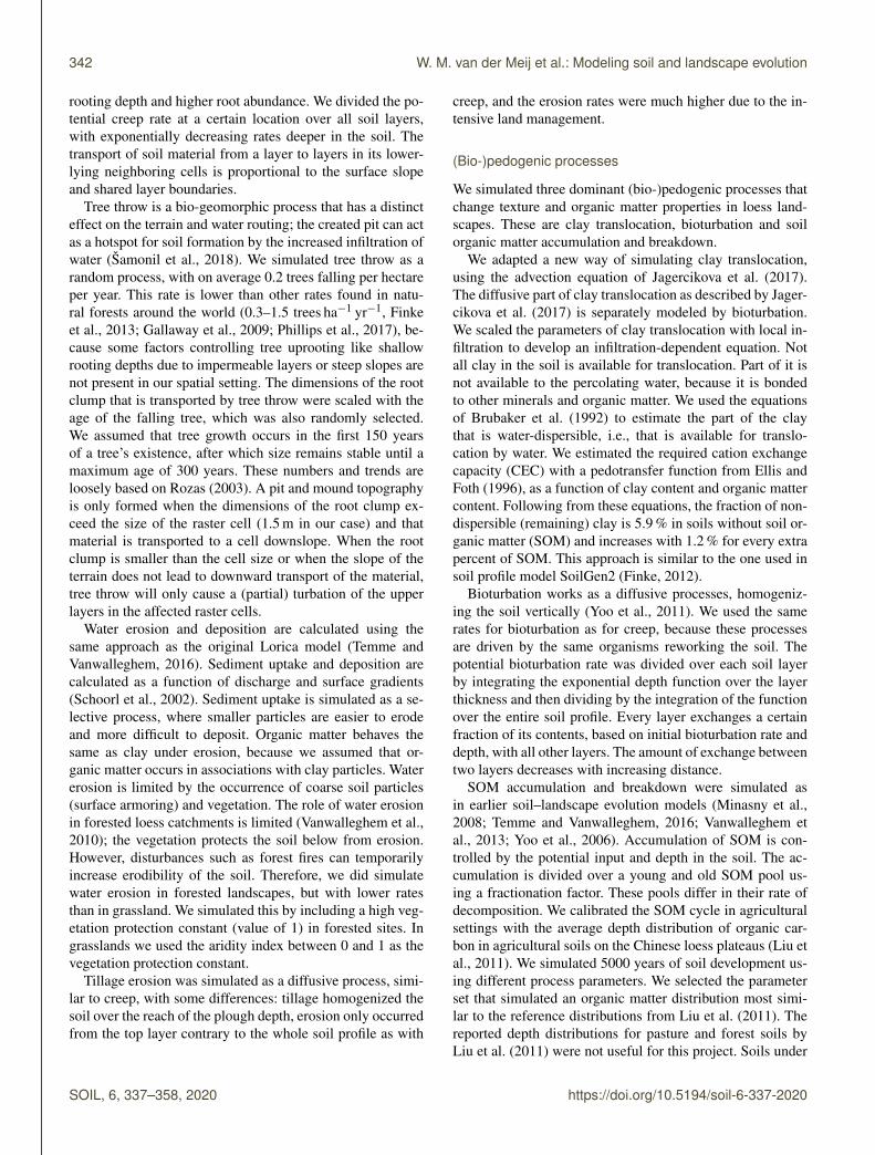
Figure 2. Transect through the catchment at the end of the natural phase and the end of the agricultural phase for the humid scenario(P = 600 mm). The black line indicates initial topography. See Fig. 1 for the location of the transect.

15× 15 cells (22.5× 22.5 m), and the topographic wetnessindex (TWI; –). In most figures, we present two moments intime. These are the end of the natural phase (t = 14500) andthe end of the agricultural phase (t = 15000). We present theresults in the following ways.

– To show the development of soils and catenae, we showtransects across the catchment (Fig. 2), and plots of soilprofile evolution, for three landscape positions and threerainfall scenarios (Fig. 3).

– To compare natural and agricultural soil properties, weshow catchment-averaged depth distributions of clayand SOM fractions (Fig. 4).

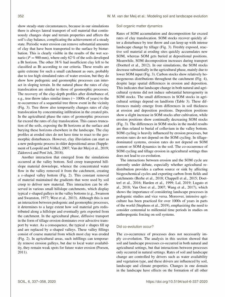
– To show the impact of geomorphic processes on the ter-rain, we show cumulative elevation changes at the endof the natural and agricultural phases, and we show con-tributions to elevation change for each geomorphic pro-cess over time (Fig. 5).

– To quantify the spatial heterogeneity of the selectedsoil and terrain properties, we calculated experimentalsemivariograms (Fig. 6), using the gstat package in R(Pebesma, 2004). Experimental semivariograms give ameasure of the variation between properties of soils asa function of distance between soils. We compared thesemivariograms of depth to the Bt horizon with semi-variograms made from field observations in a natural



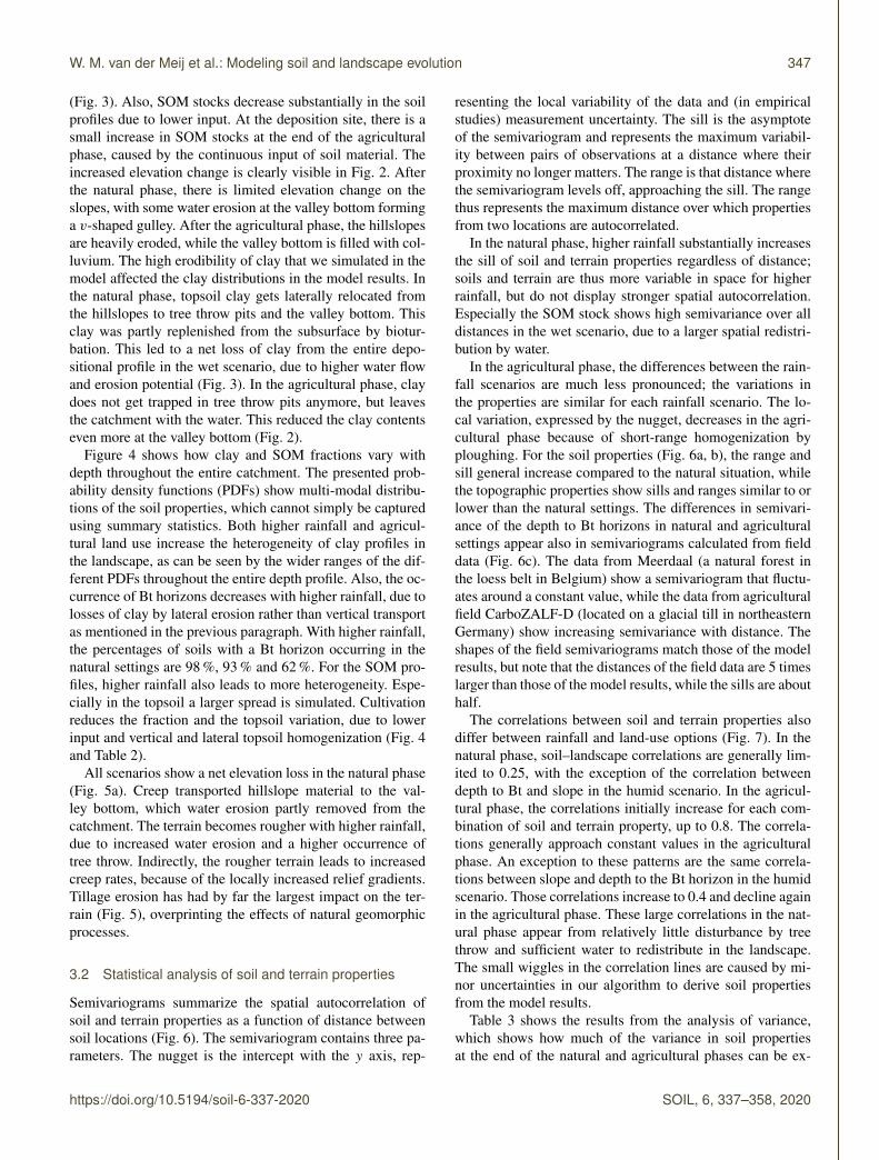
Figure 3. Evolution of soil profiles through time (x axis) on a stable, eroding and depositing position (rows), for the different rainfallscenarios (columns). The colored bars atop the plots indicate land cover (natural) and land use (agricultural). The points indicate the SOMstocks (right y axis). Note that the natural and agricultural systems have different x axis scales to visualize both systems. In the agriculturalsystem, an observation is shown every 500 years, in the agricultural phase, every 50 years. See Fig. 1 for locations of the soil profiles. SeeFig. 2 for the soil color legend.

and agricultural site. The experimental semivariogramsfrom the model results were calculated with a lag of 2 m,while the experimental semivariograms from the fielddata were calculated with a lag of 20 m.

– To visualize soil–landscape relations, we show how theselected soil properties and terrain properties are corre-lated and how these correlations change through time(Fig. 7).

– To disentangle the effects of various factors on soilproperties, we performed an analysis of variance (Ta-ble 3). We selected the depth to Bt and the carbonstock at the end of the natural and agricultural phasesas dependent variables. As independent variables weselected climate (three rainfall classes), land cover oruse (natural or agricultural), and landforms (three ele-vation classes with equal elevation ranges, representingplateau, slope and valley; Fig. 1).

3 Results

Here we present the results from the HydroLorica model.Section 3.1 shows the patterns, distributions and changes ofsoil and terrain properties in space and time. Section 3.2shows the results from the statistical analyses to quantify andsummarize spatial and temporal soil and terrain patterns. InSupplements 2 and 3 we provided two animations to help vi-sualize the simulated soil and landscape evolution. The an-imations show (1) maps of soil and terrain properties andforest cover and their changes through time, and (2) mapsof elevation change by each geomorphic process and theirchanges through time.

3.1 Simulated soil and landscape evolution

The results of HydroLorica show clear differences in the de-velopment of soil profiles at different landscape positions,for the different rainfall and land-cover/land-use scenarios(Figs. 2, 3). In the natural phase, the forest cover showsa clear climatic and topographic dependence (animation inSupplement 2). For greater rainfall, there is a higher for-



Figure 4. Probability density functions (PDFs) showing the multi-modal distributions of soil properties throughout the catchment per 10 cmdepth increment. We only show probabilities larger than 5 % for clarity. The presented soil properties are clay fraction (a, b, c) and SOMfraction (d, e, f), for the different rainfall scenarios (columns). Grey colors represent the natural soils, while red colors represent agriculturalsoils. The horizontal dotted line indicates the ploughing depth used for simulations (20 cm).

Figure 5. (a) Average erosion rates throughout the catchment for the different geomorphic processes over time. The colors represent differentgeomorphic processes, and the line types represent different rainfall scenarios. Note that the y axis is log scaled. (b) Cumulative elevationchange at the end of the natural and agricultural phase compared to the initial DEM for the different rainfall scenarios.

est cover. The spatial pattern is mainly controlled by slopeorientation. The north-facing slopes display a higher for-est cover due to lower evapotranspiration. The valley andthe hillslope depressions show a higher forest cover due tothe higher moisture availability as a consequence of surfacerunoff. Higher rainfall also leads to deeper eluviation of clayat each landscape position, showing more pronounced Bthorizons. Also, the soil profiles get more disturbed by tree

throw with higher rainfall, as can be seen by the fluctuationsin elevation and SOM stocks. The depth to the Bt horizon re-mains at the same position below the surface at the erodingposition. At all locations, SOM stocks reach an equilibriumafter ∼ 3000 years, but most of the SOM is generated in thefirst 500 years.

In the agricultural phase, relief changes much morequickly, leading to truncation of the eroding soil profile



(Fig. 3). Also, SOM stocks decrease substantially in the soilprofiles due to lower input. At the deposition site, there is asmall increase in SOM stocks at the end of the agriculturalphase, caused by the continuous input of soil material. Theincreased elevation change is clearly visible in Fig. 2. Afterthe natural phase, there is limited elevation change on theslopes, with some water erosion at the valley bottom forminga v-shaped gulley. After the agricultural phase, the hillslopesare heavily eroded, while the valley bottom is filled with col-luvium. The high erodibility of clay that we simulated in themodel affected the clay distributions in the model results. Inthe natural phase, topsoil clay gets laterally relocated fromthe hillslopes to tree throw pits and the valley bottom. Thisclay was partly replenished from the subsurface by biotur-bation. This led to a net loss of clay from the entire depo-sitional profile in the wet scenario, due to higher water flowand erosion potential (Fig. 3). In the agricultural phase, claydoes not get trapped in tree throw pits anymore, but leavesthe catchment with the water. This reduced the clay contentseven more at the valley bottom (Fig. 2).

Figure 4 shows how clay and SOM fractions vary withdepth throughout the entire catchment. The presented prob-ability density functions (PDFs) show multi-modal distribu-tions of the soil properties, which cannot simply be capturedusing summary statistics. Both higher rainfall and agricul-tural land use increase the heterogeneity of clay profiles inthe landscape, as can be seen by the wider ranges of the dif-ferent PDFs throughout the entire depth profile. Also, the oc-currence of Bt horizons decreases with higher rainfall, due tolosses of clay by lateral erosion rather than vertical transportas mentioned in the previous paragraph. With higher rainfall,the percentages of soils with a Bt horizon occurring in thenatural settings are 98 %, 93 % and 62 %. For the SOM pro-files, higher rainfall also leads to more heterogeneity. Espe-cially in the topsoil a larger spread is simulated. Cultivationreduces the fraction and the topsoil variation, due to lowerinput and vertical and lateral topsoil homogenization (Fig. 4and Table 2).

All scenarios show a net elevation loss in the natural phase(Fig. 5a). Creep transported hillslope material to the val-ley bottom, which water erosion partly removed from thecatchment. The terrain becomes rougher with higher rainfall,due to increased water erosion and a higher occurrence oftree throw. Indirectly, the rougher terrain leads to increasedcreep rates, because of the locally increased relief gradients.Tillage erosion has had by far the largest impact on the ter-rain (Fig. 5), overprinting the effects of natural geomorphicprocesses.

3.2 Statistical analysis of soil and terrain properties

Semivariograms summarize the spatial autocorrelation ofsoil and terrain properties as a function of distance betweensoil locations (Fig. 6). The semivariogram contains three pa-rameters. The nugget is the intercept with the y axis, rep-

resenting the local variability of the data and (in empiricalstudies) measurement uncertainty. The sill is the asymptoteof the semivariogram and represents the maximum variabil-ity between pairs of observations at a distance where theirproximity no longer matters. The range is that distance wherethe semivariogram levels off, approaching the sill. The rangethus represents the maximum distance over which propertiesfrom two locations are autocorrelated.

In the natural phase, higher rainfall substantially increasesthe sill of soil and terrain properties regardless of distance;soils and terrain are thus more variable in space for higherrainfall, but do not display stronger spatial autocorrelation.Especially the SOM stock shows high semivariance over alldistances in the wet scenario, due to a larger spatial redistri-bution by water.

In the agricultural phase, the differences between the rain-fall scenarios are much less pronounced; the variations inthe properties are similar for each rainfall scenario. The lo-cal variation, expressed by the nugget, decreases in the agri-cultural phase because of short-range homogenization byploughing. For the soil properties (Fig. 6a, b), the range andsill general increase compared to the natural situation, whilethe topographic properties show sills and ranges similar to orlower than the natural settings. The differences in semivari-ance of the depth to Bt horizons in natural and agriculturalsettings appear also in semivariograms calculated from fielddata (Fig. 6c). The data from Meerdaal (a natural forest inthe loess belt in Belgium) show a semivariogram that fluctu-ates around a constant value, while the data from agriculturalfield CarboZALF-D (located on a glacial till in northeasternGermany) show increasing semivariance with distance. Theshapes of the field semivariograms match those of the modelresults, but note that the distances of the field data are 5 timeslarger than those of the model results, while the sills are abouthalf.

The correlations between soil and terrain properties alsodiffer between rainfall and land-use options (Fig. 7). In thenatural phase, soil–landscape correlations are generally lim-ited to 0.25, with the exception of the correlation betweendepth to Bt and slope in the humid scenario. In the agricul-tural phase, the correlations initially increase for each com-bination of soil and terrain property, up to 0.8. The correla-tions generally approach constant values in the agriculturalphase. An exception to these patterns are the same correla-tions between slope and depth to the Bt horizon in the humidscenario. Those correlations increase to 0.4 and decline againin the agricultural phase. These large correlations in the nat-ural phase appear from relatively little disturbance by treethrow and sufficient water to redistribute in the landscape.The small wiggles in the correlation lines are caused by mi-nor uncertainties in our algorithm to derive soil propertiesfrom the model results.

Table 3 shows the results from the analysis of variance,which shows how much of the variance in soil propertiesat the end of the natural and agricultural phases can be ex-



Figure 6. Experimental semivariograms of the model results showing semivariance for different soil (a, b) and terrain properties (d–f) withdifferent precipitation scenarios (line types) at the end of the natural (black) and agricultural (red) phases. For comparison, panel (c) showsexperimental semivariograms of depth to Bt from a natural area (Meerdaal forest, P = 800 mm, Vanwalleghem et al., 2010) and an agri-cultural area (CarboZALF-D, P = 500 mm, Van der Meij et al., 2017). Note that these field data are presented with different axes. Theexperimental semivariograms are displayed with lines rather than points for easier visual comparison.

Table 2. Model and field organic carbon stocks (kg m−2) for different depth ranges, averaged over the catchment (average ± standarddeviation). The model results were converted from SOM to SOC by multiplying the SOM stocks by 0.58 (Wolff, 1864).

Carbon stocks (kg m−2)

Natural phase (t 14 500) Agricultural phase (t 15 000) Liu et al. (2011)

Depth range (m) Dry Humid Wet Dry Humid Wet(grassland) (mixed) (forest)

0–0.2 4.7± 0.3 4.6± 0.9 4.1± 2.1 2.9± 0.1 2.9± 0.3 2.8± 0.4 3.0± 1.90–0.4 8.7± 0.4 8.5± 1.1 7.8± 2.8 5.5± 0.2 5.4± 0.5 5.3± 0.6 5.4± 3.20–1 17.1± 0.4 16.8± 1.2 15.7± 3.5 10.9± 0.6 10.8± 0.8 10.6± 0.8 8.8± 4.40–2 24.1± 0.4 23.7± 1.3 22.3± 3.8 15.7± 1.2 15.6± 1.2 15.4± 1.1 14.5± 5.2Complete profile 27.7± 1.3 27.1± 1.7 25.3± 8.5 18.6± 16.1 18.4± 9.1 17.8± 10.1 –

plained by different factors (Table 3). The variance in depthto the Bt horizon can be partly explained by rainfall (18 %)and landscape position (23 %), when considering all data to-gether. However, the largest part of the variance remains un-explained. For the SOM stocks, most of the variance can beexplained by the land use (72 %). When grouped per landcover/use, about half of the variance of depth to Bt can beexplained by either rainfall (natural phase) or landform (agri-cultural phase). For the SOM stocks the dominant factors arethe same, but the variance in the natural soil landscape can

only be partly explained by rainfall (14 %), and a large partremains unexplained.

4 Discussion

4.1 Soil patterns and properties

4.1.1 Soil patterns

Soils have been affected by humans for over 1000s of years,either directly by agricultural use or indirectly by adjust-ing factors that form the soil, such as vegetation or climate



Table 3. Results from the analysis of variance, indicating the proportion of variance in soil properties explained by the different soil-formingfactors. The data are both considered in total and grouped per land use (natural or agricultural). The bold numbers indicate the largest part ofthe variance, either explained by one of the factors or unexplained. All responses are significant (p<0.05).

Depth Bt SOM stock

Total Natural Agricultural Total Natural Agricultural

Rainfall 0.18 0.49 0.08 0.02 0.14 0.02Landform 0.23 0.04 0.51 0.04 0.01 0.56Land use 0.01 – – 0.72 – –Unexplained 0.58 0.47 0.41 0.22 0.85 0.42

Figure 7. Correlations (R2) between selected soil properties (linetypes) and topographic properties (colors) through time (left toright), for the different rainfall scenarios (top to bottom). In thenatural system, the correlations are presented every 500 years,while in the agricultural system, the correlations are presented every50 years. Note that for the latter phase the x axis is stretched.

(Amundson et al., 2015; Bajard et al., 2017; Dotterweich,2008; Stephens et al., 2019). Therefore it is difficult, if notimpossible, to find locations where truly natural soils can beobserved and compared to agricultural soils in similar set-tings. Model simulations enable this comparison, as we showin this study. Unfortunately, there are limited field data to cal-ibrate and validate the model. To our knowledge, the datasetfrom Vanwalleghem et al. (2010) is the only dataset that en-ables quantification of the spatial distribution of natural soilsand links it to terrain properties at a local to regional scale,similar to the setting we simulated. In this section, we relymainly on this dataset to discuss and evaluate the patternsof natural soils we simulated with our model. For the agri-

cultural soil patterns, we use an extensive dataset from an in-tensively managed agricultural field in northeastern Germany(CarboZALF-D, Van der Meij et al., 2017). In our model sim-ulations, we simplified the agricultural conversion by assum-ing a single vegetation type in the entire catchment and directintensive management with tillage. This enabled us to isolatethe role of tillage erosion in the development of agriculturalsoil and landscape patterns. We did not consider a slow his-torical development of the agricultural system with increas-ing management intensity and upscaling of agricultural fieldsizes. The results of our simulations should be consideredto be within-field variation in soil and landscape properties.In smaller-scale farming, the within-field soil–landscape re-lations will also be present, but they are probably secondaryto variation between fields caused by different management(history), vegetation type or anthropogenic structures such ashedges, banks and roads (e.g., Follain et al., 2006; Peukert etal., 2016; Yemefack et al., 2005).

We used semivariograms to illustrate the spatial autocor-relation of soil and landscape properties (Fig. 6). Semivari-ograms are very case-study-specific, because the range, silland nugget are affected by the scale of topographic andlithogenic variation, different rates of pedogenic and geomor-phic processes and different types of human disturbances inthe landscape. Therefore, we only compare the trends in thesemivariograms from model and field results to evaluate thetype of spatial autocorrelation of soil properties in such set-tings.

Figure 6b and c show experimental semivariograms ofdepths to Bt horizons in model and field data. In both pan-els, the agricultural settings show higher spatial autocorrela-tion compared to the natural settings, expressed by the highersill and range. This indicates that in agricultural fields thedepths to Bt horizons are more spatially organized (higherlarge-scale variability), with larger differences between dif-ferent landscape positions. In natural areas, the spatial differ-ences in depth to Bt horizon are lower and there is less spatialorganization of the depth distributions. The model and fieldresults show different magnitudes in nugget, range and sill.This can be explained by (1) the high density of data pointsin the model results which enabled us to calculate the semi-variance over very short distances, reducing the nugget, and



(2) the fact that we used a very condensed DEM with high lo-cal variation in topographic properties as input for the modelresults, which led to high local variation in soil propertiestoo. Nonetheless, the similar trends in the field and modelsemivariograms indicate that the general soil patterns frommodel and field results agree. Also, the correlations betweensoil and landscape properties are similar for field and modelresults. Vanwalleghem et al. (2010) found correlations be-tween different horizon depths and topographic propertieswith R2s ranging between 0.02 and 0.1, which are the sameorder as most correlations we calculated in Fig. 7. These sim-ilarities indicate that our model HydroLorica simulated theessential processes that form these natural soil patterns.

Our simulations show a large diversity of natural soil pat-terns, influenced by the amount of rainfall and associatedvegetation type. The available water leads to a regionallyhigher rate of soil development, for example in the form ofdeeper clay eluviation (Fig. 3), and also to a greater lateral re-distribution of soil material by water erosion and tree throw(Fig. 5) and spatially varying infiltration rates. With morerainfall, the higher rates and interactions between these pro-cesses lead to a spatially more heterogeneous soil pattern, asexpressed in higher ranges and sills in the semivariograms(Fig. 6). This local variation in pedogenesis due to differ-ent water input has been recognized and partly accountedfor in other modeling studies (Finke et al., 2013; Saco etal., 2006; Shepard et al., 2017), but had not emerged fromsoil–landscape evolution studies. Also, the terrain, summa-rized by slope, TPI and TWI, becomes more heterogeneouswith higher rainfall. Water flow thus affects soil and terrainpatterns in a similar way.

Intensively managed agricultural soils display entirely dif-ferent patterns compared to natural soils. There is lowersmall-scale variability due to the absence of tree throw andlocal homogenization by tillage, while the semivariogramsof soil properties suggest higher sills, i.e., higher large-scalevariability and spatial autocorrelation of soil properties com-pared to natural soil properties. This is due to the slope-dependent intensity of tillage erosion (Phillips et al., 1999).This erosion leads to truncation of soils at convex positions,while concave positions have a net accumulation of material(De Alba et al., 2004). This truncation is visible in many agri-cultural landscapes, because subsurface horizons with differ-ent colors get exposed at the surface in heavily eroded lo-cations (e.g., Smetanová, 2009; Van der Meij et al., 2017).In contrast, terrain properties seem to display lower spatialvariation in agricultural landscapes. The smoothing effect oftillage on the terrain removed local pits and rills created inthe natural phase. We hypothesized earlier that a smootherterrain would have higher hillslope connectivity, leading toincreased water erosion (Van der Meij et al., 2017). How-ever, we observed the contrary in our model results (Fig. 5).The export of sediments from the catchment might be higher,but the uptake and local redistribution of sediments on thehillslope is lower, because local steep gradients are removed.

Tillage is thus the dominant process forming agricultural soilpatterns. The effect of anthropogenic soil erosion on soil het-erogeneity far exceeds effects of changes in for example rain-fall, which shows the huge impact we have as humans onsoil–landscape development.

4.1.2 Process calibration and verification

The rates of the simulated processes were difficult to cali-brate and validate. This is mainly due to a lack of field datathat cover a range of climatic, topographic, chronologic andgeographic settings (Van der Meij et al., 2018). Such dataare essential for formulating pedogenic functions that are ap-plicable in a wide range of settings instead of only in casestudies, or for verifying model results. The chronosequencecollection of Shepard et al. (2017) is a global dataset of soilsin various settings covering different time steps. This datasetcould be a good starting point for developing such func-tions owing to its large coverage. But as chronosequencesare generally situated in relatively flat, stable landscapes,they often do not contain information about variations of soilproperties at small distances, as a function of local terrain(Harden, 1988; Sauer, 2015) – with the exception of somepro-glacial soil chronosequences whose use is limited be-cause of their extreme climate and parent material (Egli etal., 2006; Temme and Lange, 2014). Such more complete in-formation is essential for understanding the formation of soilpatterns, as illustrated in the previous section. Therefore, wesuggest including topographic variation in future chronose-quence studies (Temme, 2019). A dataset covering differentgeographies could also raise the comparison of model andfield results beyond the case-study level.

In this study, we worked with an artificial landscape toavoid effects of uncertainties and local variations in initialand boundary conditions that are often present in data fromfield settings (e.g., Van der Meij et al., 2017). This allowedus to investigate the universal effects of changes in rainfalland land use on the model results, as a function of terrainmorphology. Although uncertainties in boundary conditionsappear to have a limited effect on the outcomes of soil evo-lution models, uncertainties in initial conditions can stronglyinfluence the results (Keyvanshokouhi et al., 2016).

One soil property for which there are plenty of data on thespatiotemporal variation is soil organic matter or carbon, dueto the current interest in its potential to store atmosphericcarbon (Minasny et al., 2017). We used a regional datasetfrom the loess plateau to calibrate our SOM cycle in agri-cultural landscapes, and we used carbon sequestration ratesfor adjusting the SOM balances for forest and grassland ar-eas. The modeled SOM stocks for agricultural sites matchthe field data fairly well (Table 2), but stocks for natural ar-eas are estimated higher than often observed. For example, inBavaria, Germany, carbon stocks in the first meter, includingthe optional litter layer, are 9.8–11.8 kg m−2 (Wiesmeier etal., 2012), where we simulated 15.7–17.1 kg m−2 in our nat-



ural settings without consideration of a litter layer. Also, thedepth distributions are different. De Vos et al. (2015) foundthat 50 % of the carbon stock occurs in the top 20 cm in Eu-ropean forests on various parent materials. In our results thisis around 20 %. This implies that agriculturally derived SOMdepth functions are not suitable for calibrating natural SOMdepth functions, probably because input, vertical redistribu-tion, litter quality and decay of SOM behave differently innatural and agricultural sites. To calibrate these parameters,data from agricultural and natural sites in close vicinity areneeded to avoid effects of geographic and climatic differ-ences. We are currently not able to simulate and calibratethese processes properly.

4.2 Drivers of soil formation

4.2.1 Soil-forming factors

Different soil-forming factors dominate the variance in soilproperties in natural and agricultural systems (Table 3). Innatural systems, rainfall is the dominant factor explainingthe variance. In scenarios with greater rainfall, rates of soiland landscape change are larger, leading to more complexpatterns. Although we did not simulate a changing climate,the results suggest that we can expect more stable conditionswith similar pedogenesis rates throughout the landscape inperiods with lower rainfall, while periods with greater rain-fall may induce landscape change and spatially varying ratesof pedogenesis. The major driver of this increased landscapechange is the higher occurrence of tree throw. The higherwater availability increases forest cover, leading to more treethrows (see the animations in Supplements 2 and 3).

Although our vegetation module is very simple, it was ableto simulate the climatic and topographic control on vegeta-tion patterns which affect geomorphic and pedogenic pro-cesses. We would expect similar results to be obtained if amore complex vegetation module that does justice to ecolog-ical complexity (i.e., resilience, succession) would be incor-porated.

In intensive agricultural systems with large fields, land-form is the dominant factor explaining the variance (Ta-ble 3). This shift from external factors in natural systemsto internal factors in agricultural systems marks the impor-tance of geomophic processes in agricultural soil patterns.Although relief controls rates and directions of geomorphicprocesses, the type of process is human-controlled. Humanshave a massive impact on soil development (Amundson andJenny, 1991; Dudal, 2005). Direct effects include agricul-tural use, excavations, introduction of organisms and cre-ation of new parent materials (Richter et al., 2015), whileindirectly anthropogenic changes in climate can have severeeffects on soil properties (Nearing et al., 2004; Schuur et al.,2015). We have focussed on the main of these anthropogenicchanges in loess landscapes: removal of forest and com-plete introduction of tillage, even though intermediate forms

with incomplete clearing, smaller fields and forested bordersmay have historically existed. Humans as soil-forming fac-tors form new catenae (anthroposequences) and soil patterns,where the ultimate pattern only depends little on the initialvariation (Fig. 6). In our model results, we observe four ofthe six anthropogenic changes to soils, as described by Du-dal (2005): human-made soil horizons, deep soil disturbance,topsoil changes and changes in landforms. These changessubstantially affect soil functions, such as biodiversity andfood security. Our simulations thus support the view that hu-mans are the dominant factor in forming soils in agriculturallandscapes.

4.2.2 Soil–landscape (co-)evolution

The development of soils and landscapes is not merely acollection of individual processes, but also of interactionsbetween different processes. When processes interact, andwhen changes to soils and landscapes are on the same orderof magnitude, soil–landscape co-evolution can occur. Thisco-evolution can amplify or diminish certain processes or cancompletely change the direction of soil and landscape evolu-tion (Van der Meij et al., 2018). Often, co-evolution is usedto describe soil and landscape processes with similar ratesbut that do not necessarily interact (e.g., Willgoose, 2018).This would imply that these processes would co-occur ratherthan co-evolve. In this section we evaluate some co-occurringprocesses in HydroLorica to see whether co-evolution oc-curred. There are different co-occurring processes in the nat-ural phase of slow landscape change compared to the agri-cultural phase of intense landscape change.

Lateral and vertical transport

We will first consider vertical and lateral soil transport pro-cesses. Soils and hillslopes can be considered a series oftransport ways or conveyor belts (Román-Sánchez et al.,2019). Vertical transport or mixing occurs by bioturbationincluding tree throw and clay translocation, whereas lat-eral transport occurs by creep, tree throw, water erosionand tillage erosion. Interactions between processes can occurwhere transport ways affect the same material. Two exam-ples we will discuss here are the vertical and lateral transportof clay and the interaction between creep and water erosionin the valley bottom.

The vertical translocation of clay is simulated in our modelby an advection–diffusion equation, where the advective partis the downward transport by water flow and the diffu-sive part a homogenization by bioturbation (Jagercikova etal., 2017). When the rates of advection and diffusion areequal, the upward transport of clay by bioturbation equals theamount of downward translocation by water; the clay-depthprofile of the soil occurs in steady state and will not changesubstantially. Steady-state circumstances are however rare innatural soil systems (Phillips, 2010). Our simulations do not



show steady-state circumstances, because in our simulationsthere is always lateral transport of soil material that contin-uously changes slope and terrain properties and affects thesoil’s clay balance, complicating the achievement of a steadystate. Periodic water erosion can remove substantial amountsof clay that have been transported to the surface by biotur-bation. This is clearly visible in the results of the wet sce-nario (P = 900 mm), where only 62 % of the soils developeda Bt horizon. The other 38 % had insufficient clay left to beclassified as Bt according to our criteria. These results arequite extreme for such a small catchment as ours, probablydue to too high simulated rates of water erosion, but they doshow how pedogenic and geomorphic processes can inter-act in sloping terrain. In the natural phase the rates of claytranslocation are similar to those of geomorphic processes.The recovery of the clay-depth profiles after disturbance of,e.g., tree throw takes similar times (∼ 1000s of years) to there-occurrence of a sequential tree throw event in the vicinity(Fig. 3). Tree throw also temporarily changes rates of claytranslocation by concentrating infiltration in the created pits.In the agricultural phase the rates of geomorphic processesfar exceed the rates of clay translocation. This causes trunca-tion of the soils, exposing the Bt horizons at the surface andburying these horizons elsewhere in the landscape. The clayprofiles at eroded sites do not have time to react to the geo-morphic disturbances. However, clay illuviation can start asa new pedogenic process in older depositional areas (Supple-ment of Leopold and Völkel, 2007; Van der Meij et al., 2019;Zádorová and Pení žek, 2018).

Another interaction that emerged from the simulationsoccurred at the valley bottom. Soil creep transported hill-slope material downslope, whence the concentrated waterflow in the valley removed it from the catchment, creatinga v-shaped valley bottom (Fig. 2). This constant removalof material maintained the gradients that were used by soilcreep to deliver new material. This interaction can be ob-served in various small hillslope catchments, which displaytypical v-shaped gulleys in the valley bottoms (e.g., Swansonand Swanston, 1977; West et al., 2013). Although this is notan interaction between pedogenic and geomorphic processes,it determines to a large extent how soil material gets redis-tributed along a hillslope and eventually gets exported fromthe catchment. In the agricultural phase, diffusive transportin the form of tillage erosion dominates over advective trans-port by water. As a consequence, the typical v shapes fill upand are replaced by u-shaped valleys. These valley fillingsconsist of coarse material from which most clay was eroded(Fig. 2). In agricultural areas, such infillings can temporar-ily remove erosion gulleys, but due to local water availabil-ity, they remain weak spots for future water erosion (Poesen,2011).

Soil organic matter dynamics

Rates of SOM accumulation and decomposition far exceedrates of clay translocation. SOM stocks recover quickly af-ter a disturbance by tree throw and can keep up with intenselandscape change by tillage (Fig. 3). Freshly exposed, reac-tive soil material at eroding sites quickly accumulates newSOM, whereas SOM gets buried at depositional positions.Meanwhile, SOM decomposition increases during transport(Doetterl et al., 2012). In our simulations, the SOM stocksdecrease substantially in the agricultural phase, mainly due tolower SOM input (Fig. 3). Carbon stocks show relatively ho-mogeneous distributions throughout the catchment (Fig. 4),despite large spatial differences in erosion and deposition.This indicates that landscape change in both natural and agri-cultural systems did not induce substantial heterogeneity inSOM stocks. The small differences in SOM stocks in agri-cultural settings depend on landform (Table 3). These dif-ferences mainly emerge from differences in soil thicknessat erosion and deposition positions. Deposition positionsshow a slight increase in SOM stocks after cultivation, whileerosion positions show continually decreasing SOM stocks(Fig. 3). The differences in SOM stocks in the model resultsare thus related to burial of colluvium in the valley bottom.SOM cycling is heavily influenced by erosion processes, buterosion rates do not depend on the SOM cycling. In tillage-dominated systems, erosion rates do not depend on SOMcontent or SOM dynamics in the soil. The co-occurrence ofSOM cycling and tillage erosion in agricultural settings thusdoes not lead to co-evolution.

The interactions between erosion and the SOM cycle arecurrently under debate, especially whether agricultural re-distribution provides a carbon source or sink by affectingbiogeochemical cycles and exporting carbon from fields andcatchments (Berhe et al., 2018; Chappell et al., 2015; Doet-terl et al., 2016; Harden et al., 1999; Lal, 2019; Lugato etal., 2018; Van Oost et al., 2007; Wang et al., 2017), whichshows the importance of considering landscape processes inpedogenic studies and vice versa. Moreover, intensive agri-culture has been practiced for over 1000s of years in partsof the world (Stephens et al., 2019), emphasizing the need toconsider centennial to millennial time periods in studies onanthropogenic forcing on soil systems.

Did co-evolution occur?

The co-occurrence of processes does not necessarily im-ply co-evolution. The analysis in this section showed thatsoil and landscape processes co-occurred in both natural andagricultural settings, but that interactions between processesonly occurred in natural settings. Rates of soil and landscapechange are controlled by drivers such as water availabilityand vegetation type, and these drivers are influenced by soil,landscape and climate properties. Changes in one domainin the landscape have effects on the formation of all other



domains. These interactions, or co-evolution, occur on bothshort and long timescales in the natural system. There arealready considerable differences between the soil patternsfrom each scenario after 500 years of natural soil formation,due to the role of water and vegetation in soil–landscape co-evolution. These differences become more pronounced overtime, due to progressive soil and landscape formation (Sup-plement 2).

In comparison, the differences between the patterns ofeach scenario after 500 years of agricultural land use aremuch smaller (Supplement 2). This is because anthropogenicprocesses such as tillage erosion occur at such high rates thatmost natural processes cannot keep up and lead to more sim-ilar soil landscapes. In settings with uniform parent mate-rial such as we simulated, anthropogenic processes do notshow co-evolution, because the rates of for example tillageerosion far exceed any rates of natural soil and landscapechange (Fig. 5), and the rates of the anthropogenic processesare not influenced by soil properties. Tillage can introducenew processes or accelerate other processes, e.g., by break-ing up aggregates. However, these processes do not affectthe rate at which a plough transports sediments through alandscape. If interactions between processes do not occuron shorter timescales, they will also not emerge over longertimescales, as is the case with natural processes as describedbefore. The occurrence of possible co-evolution of soils andlandscapes thus depends on the type of processes that affectthe system, not on the duration over which these processeschange soils and landscapes. In other words, co-evolution isnot time-dependent, but process-dependent.

Co-evolution of soils and landscapes can also occur via in-trinsic thresholds which do not depend on changes in exter-nal drivers such as rainfall and land use. An example is thedevelopment of stagnating layers in the soil, which changethe subsurface partitioning of water and can introduce re-ducing conditions. But, as we explain in Van der Meij etal. (2018), such intrinsic thresholds can currently not be mod-eled, because we lack the methods for estimating accuratesoil hydraulic properties which drive this threshold behavior.Ideally, a model shows such threshold behavior without ex-plicitly incorporating these thresholds into the model codeas such imposed hard thresholds can cause problems whencalibrating the model by creating sharp discontinuities in themodel results as a response to slight variations in parameters(Barnhart et al., 2019). For these reasons we focused on het-erogeneity and (co-)evolution related to external drivers inthis research.

The soil and landscape interactions in natural settings em-phasize the need to study natural soil formation in a land-scape context rather than a pedon context. Only when land-scapes are stable, flat and free of trees are changes in soilproperties not influenced by changes in terrain. In such set-tings, a 1D soil profile evolution model would suffice tosimulate soil development in different landscape positions(Finke, 2012; Minasny et al., 2015). When rates of geomor-

phic processes far exceed those of pedogenic processes, forexample in tillage-dominated systems, a landscape evolutionmodel would suffice (e.g., Temme et al., 2017). In undulat-ing landscapes where various hillslope processes occur, soilsshould be considered 3D bodies, and soil–landscape evolu-tion models are essential to simulate spatial drivers of soiland landscape evolution (Willgoose, 2018).

4.3 Predictability of soil patterns

In digital soil mapping, empirical relations between soilproperties and their environment are used to predict soilproperties through space (McBratney et al., 2003). In orderto predict soil properties with environmental variables, theenvironmental variables should show variation over the samespatial scale as the variable to be predicted. On a hillslopescale, this variation often occurs in terrain properties (Gessleret al., 2000), while external factors such as climate often donot vary spatially at these scales. The shift from dominant ex-ternal to dominant internal soil-forming factors in explainingvariance in observed soil properties (Table 3) thus has largeimplications for our ability to predict and map soil patterns.Human activity has created soil landscapes that are well-suited for digital soil mapping. The correlations betweensimulated soil and several terrain properties all give the samesignal (Fig. 7): the correlations in the natural phase are lim-ited, but increase rapidly in the agricultural phase. The switchfrom a natural to agricultural phase thus increases soil het-erogeneity, but also soil predictability, which can be used topredict the soil properties in large-field settings. One shouldbe careful extrapolating soil-terrain relationships from agri-cultural areas to natural areas, as these correlations dependon land management and can give wrong results under dif-ferent land cover.

Digital soil mapping (DSM) performs well when predict-ing the spatial distribution of agricultural soils, but its appli-cability in time is limited because of limited temporal data(Gasch et al., 2015; Grunwald, 2009). The limited obser-vations in space and time can be supplemented or extrapo-lated by incorporating biogeochemical process descriptionsto improve DSM (Angelini et al., 2016; Christakos, 2000, 22pp.; Heuvelink and Webster, 2001). However, the responseof soils and terrains to changes in soil-forming factors takeslonger (decades to millennia) than the time span over whichwe have observations (days to decades). Process-based mod-els thus become increasingly essential for understanding howsoils might change under projected scenarios of land use andclimate change (Keyvanshokouhi et al., 2016; Opolot et al.,2015), and HydroLorica shows a promising first example ofsuch a model on a landscape scale that responds to changesin all five soil-forming factors and by extension the humancontrol on these factors.



5 Conclusions

Soils undergo substantial changes in the transition from anatural land cover to agricultural land use. Although thesechanges can be described conceptually, quantitative data todescribe the changes in soil pattern are scarce. We devel-oped a soil–landscape evolution model, named HydroLor-ica, which is able to simulate the evolution of soils and land-scapes in both natural and agricultural settings, by simulatingspatially varying infiltration as a driver of soil formation andby inclusion of essential natural and agricultural processessuch as soil creep, tree throw and tillage. We used this modelto simulate soil and landscape development in varying cli-matic settings, under changing land use, to quantify changesin variation and predictability of soil patterns. We reachedthe following conclusions.

– Natural and agricultural landscapes display differentsoil patterns. Natural soil patterns are more chaotic andrandom with higher precipitation. Their formation isdominated by local processes such as tree throw andspatially varying infiltration. Soil patterns in intensivelymanaged fields are dominantly formed by tillage ero-sion processes. Also, agricultural soil properties showlarger correlations with terrain properties.

– In natural systems, rainfall is the main factor influenc-ing soil variation. In agricultural systems, landform ex-plains the largest part of variation. The most importantfactor affecting total soil variation is the human fac-tor. Agricultural land use increases erosion rates, whichchanges soil patterns and creates and amplifies the to-pographic dependence of soil properties.

– In natural and agricultural settings there are differentsets of processes that change soils and landscape withsimilar rates. In natural systems, these processes of-ten interact and amplify or diminish each other, leadingto soil–landscape co-evolution. In agricultural systems,these interactions are often missing, and processes co-occur rather than co-evolve.

– Agricultural soil patterns in a large-field setting are eas-ier to predict than natural soil patterns, due to the shiftfrom dominant external to internal factors that explainsoil variation, which manifests itself in larger correla-tions between soil and terrain properties.

Soil–landscape evolution models are increasinglyequipped to simulate soil–landscape development in avariety of settings. Our contribution shows the added valueof using water availability as a spatially varying driver ofpedogenesis to simulate soil and landscape development innatural settings. These developments are essential to studythe vulnerability and resilience of soil systems under theincreasing pressure from land-use intensification and thechanging climate, but can also assist in understanding the

long-term effects of management strategies such as reducedtillage or no-till on soil properties such as carbon stocks.

Code and data availability. Model code is available on requestvia the corresponding author. Weather data that were used to runthe model were gathered from the Deutscher Wetterdienst (DWDClimate Data Center (CDC), 2018a, b).

Supplement. We provided the following Supplements: Sup-plement 1: Model equations and parameters (document). Sup-plement 2: Maps of soil and terrain properties through time(animation). Supplement 3: Maps of elevation change dueto the different geomorphic processes through time (anima-tion). The supplement related to this article is available onlineat: https://doi.org/10.5194/soil-6-337-2020-supplement.

Author contributions. The authors contributed to experimentalconcept and design, model development, data analysis and paperpreparation in the following proportions: WMvdM (25 %, 75 %,75 %, 65 %), AJAMT (25 %, 25 %, 15 %, 20 %), JW (25 %, 0 %,10 %, 10 %), MS (25 %, 0 %, 0 %, 5 %). The authors declare thatthey have no conflict of interest.

Competing interests. The authors declare that they have no con-flict of interest.

Acknowledgements. We thank Tom Vanwalleghem (Universityof Cordoba, Spain) for sharing the Meerdaal dataset.

Review statement. This paper was edited by Peter Fiener and re-viewed by Christopher Shepard and one anonymous referee.

References

Alewell, C., Egli, M., and Meusburger, K.: An attempt to estimatetolerable soil erosion rates by matching soil formation with de-nudation in Alpine grasslands, J. Soil. Sediment., 15, 1383–1399,2015.

Allen, R. G., Pereira, L. S., Raes, D., and Smith, M.: Cropevapotranspiration-Guidelines for computing crop water require-ments, Irrigation and drainage paper 56, FAO, Rome, 1998.

Amundson, R. and Jenny, H.: The place of humans in the state fac-tor theory of ecosystems and their soils, Soil Sci., 151, 99–109,1991.

Amundson, R., Berhe, A. A., Hopmans, J. W., Olson,C., Sztein, A. E., and Sparks, D. L.: Soil and humansecurity in the 21st century, Science, 348, 1261071,https://doi.org/10.1126/science.1261071, 2015.

Angelini, M. E., Heuvelink, G. B. M., Kempen, B., and Morrás, H.J. M.: Mapping the soils of an Argentine Pampas region usingstructural equation modelling, Geoderma, 281, 102–118, 2016.


https://doi.org/10.5194/soil-6-337-2020-supplement

https://doi.org/10.1126/science.1261071


Bai, Z. G., Dent, D. L., Olsson, L., and Schaepman, M. E.: Proxyglobal assessment of land degradation, Soil Use Manage., 24,223–234, 2008.

Bajard, M., Poulenard, J., Sabatier, P., Develle, A.-L., Giguet-Covex, C., Jacob, J., Crouzet, C., David, F., Pignol, C., and Ar-naud, F.: Progressive and regressive soil evolution phases in theAnthropocene, CATENA, 150, 39–52, 2017.

Barnhart, K. R., Glade, R. C., Shobe, C. M., and Tucker, G. E.:Terrainbento 1.0: a Python package for multi-model analysisin long-term drainage basin evolution, Geosci. Model Dev., 12,1267–1297, https://doi.org/10.5194/gmd-12-1267-2019, 2019.

Berhe, A. A., Barnes, R. T., Six, J., and Marín-Spiotta, E.: Role ofSoil Erosion in Biogeochemical Cycling of Essential Elements:Carbon, Nitrogen, and Phosphorus, Annu. Rev. Earth Pl. Sc., 46,521–548, 2018.

Bibby, J. S. and Mackney, D.: Land use capability classification,Rothamsted Experimental Station, Harpenden, England, 27 pp.,1969.

Bouma, J.: Soil science contributions towards sustainable develop-ment goals and their implementation: linking soil functions withecosystem services, J. Plant Nutr. Soil. Sc., 177, 111–120, 2014.

Brubaker, S. C., Holzhey, C. S., and Brasher, B. R.: Estimating thewater-dispersible clay content of soils, Soil Sci. Soc. Am. J., 56,1226–1232, 1992.

Budyko, M. I. and Miller, D. H.: Climate and life, Academic press,New York, 507 pp., 1974.

Catt, J. A.: The agricultural importance of loess, Earth-Sci. Rev.,54, 213–229, 2001.

Chappell, A., Baldock, J., and Sanderman, J.: The global signifi-cance of omitting soil erosion from soil organic carbon cyclingschemes, Nat. Clim. Change, 6, 187–191, 2015.

Chen, S., Richer-de-Forges, A. C., Saby, N. P. A., Martin, M. P.,Walter, C., and Arrouays, D.: Building a pedotransfer functionfor soil bulk density on regional dataset and testing its validityover a larger area, Geoderma, 312, 52–63, 2018.

Christakos, G.: Modern spatiotemporal geostatistics, Oxford Uni-versity Press, Oxford, 312 pp., 2000.

Cowie, A. L., Orr, B. J., Castillo Sanchez, V. M., Chasek, P., Cross-man, N. D., Erlewein, A., Louwagie, G., Maron, M., Metternicht,G. I., Minelli, S., Tengberg, A. E., Walter, S., and Welton, S.:Land in balance: The scientific conceptual framework for LandDegradation Neutrality, Environ. Sci. Pol. 79, 25–35, 2018.

De Alba, S., Lindstrom, M., Schumacher, T. E., and Malo, D. D.:Soil landscape evolution due to soil redistribution by tillage: anew conceptual model of soil catena evolution in agriculturallandscapes, CATENA, 58, 77–100, 2004.

De Vos, B., Cools, N., Ilvesniemi, H., Vesterdal, L., Vanguelova,E., and Carnicelli, S.: Benchmark values for forest soil carbonstocks in Europe: Results from a large scale forest soil survey,Geoderma, 251/252, 33–46, 2015.

Doetterl, S., Six, J., Van Wesemael, B., and Van Oost, K.: Car-bon cycling in eroding landscapes: geomorphic controls on soilorganic C pool composition and C stabilization, Glob. ChangeBiol., 18, 2218–2232, 2012.

Doetterl, S., Berhe, A. A., Nadeu, E., Wang, Z., Sommer, M.,and Fiener, P.: Erosion, deposition and soil carbon: A review ofprocess-level controls, experimental tools and models to addressC cycling in dynamic landscapes, Earth-Sci. Rev., 154, 102–122,2016.

Dominati, E., Patterson, M., and Mackay, A.: A framework for clas-sifying and quantifying the natural capital and ecosystem ser-vices of soils, Ecol. Econ., 69, 1858–1868, 2010.

Dotterweich, M.: The history of soil erosion and fluvial deposits insmall catchments of central Europe: Deciphering the long-terminteraction between humans and the environment – A review, Ge-omorphology, 101, 192–208, 2008.

Dudal, R.: The sixth factor of soil formation, Euras. Soil Sci., 38,S60–S65, 2005.

Dürr, H. H., Meybeck, M., and Dürr, S. H.: Lithologic composi-tion of the Earth’s continental surfaces derived from a new digitalmap emphasizing riverine material transfer, Global Biogeochem.Cy., 19, GB4S10, https://doi.org/10.1029/2005GB002515, 2005.

DWD Climate Data Center (CDC): Historical daily stationobservations (temperature, pressure, precipitation, sunshineduration, etc.) for Germany, version v006, available at:https://opendata.dwd.de/climate_environment/...air_temperature/,2018a.

DWD Climate Data Center (CDC): Historical hourly station obser-vations of precipitation for Germany, version v006, available at:https://opendata.dwd.de/climate_environment/...precipitation/,2018b.

Egli, M., Wernli, M., Kneisel, C., and Haeberli, W.: Melting glaciersand soil development in the proglacial area Morteratsch (SwissAlps): I. Soil type chronosequence, Arct. Antarct. Alp. Res., 38,499–509, 2006.

Ellis, B. and Foth, H.: Soil fertility, CRC Press, Boca Raton, Florida,290 pp., 1996.

Fick, S. E. and Hijmans, R. J.: WorldClim 2: new 1-km spatial reso-lution climate surfaces for global land areas, Int. J. Climatol., 37,4302–4315, 2017.

Finke, P. A.: Modeling the genesis of luvisols as a function of to-pographic position in loess parent material, Quaternary Int., 265,3–17, 2012.

Finke, P. A., Vanwalleghem, T., Opolot, E., Poesen, J., and Deck-ers, J.: Estimating the effect of tree uprooting on variation of soilhorizon depth by confronting pedogenetic simulations to mea-surements in a Belgian loess area, J. Geophys. Re.-Earth Sur.,118, 2124–2139, 2013.

Follain, S., Minasny, B., McBratney, A. B., and Walter, C.: Simu-lation of soil thickness evolution in a complex agricultural land-scape at fine spatial and temporal scales, Geoderma, 133, 71–86,2006.

Gabet, E. J., Reichman, O. J., and Seabloom, E. W.: The effectsof bioturbation on soil processes and sediment transport, Annu.Rev. Earth Pl. Sc., 31, 249–273, 2003.

Gallaway, J. M., Martin, Y. E., and Johnson, E. A.: Sediment trans-port due to tree root throw: integrating tree population dynamics,wildfire and geomorphic response, Earth Surf. Proc. Land., 34,1255–1269, 2009.

Gasch, C. K., Hengl, T., Gräler, B., Meyer, H., Magney, T. S., andBrown, D. J.: Spatio-temporal interpolation of soil water, tem-perature, and electrical conductivity in 3D+T: The Cook Agron-omy Farm data set, Spat. Stat.-Neth., 14, 70–90, 2015.

Gessler, P. E., Chadwick, O. A., Chamran, F., Althouse, L., andHolmes, K.: Modeling Soil–Landscape and Ecosystem Proper-ties Using Terrain Attributes, Soil Sci. Soc. Am. J., 64, 2046–2056, 2000.


https://doi.org/10.5194/gmd-12-1267-2019

https://doi.org/10.1029/2005GB002515

https://opendata.dwd.de/climate_environment/CDC/observations_germany/climate/hourly/air_temperature/historical/stundenwerte_TU_01869_19810101_20191231_hist.zip

https://opendata.dwd.de/climate_environment/CDC/observations_germany/climate/hourly/precipitation/historical/stundenwerte_RR_01869_19950901_20191231_hist.zip


Greiner, L., Keller, A., Grêt-Regamey, A., and Papritz, A.: Soilfunction assessment: review of methods for quantifying the con-tributions of soils to ecosystem services, Land Use Policy, 69,224–237, 2017.

Grunwald, S.: Multi-criteria characterization of recent digital soilmapping and modeling approaches, Geoderma, 152, 195–207,2009.

Guo, L. B. and Gifford, R. M.: Soil carbon stocks and land usechange: a meta analysis, Glob. Change Biol., 8, 345–360, 2002.

Harden, J. W.: Genetic interpretations of elemental and chemicaldifferences in a soil chronosequence, California, Geoderma, 43,179–193, 1988.

Harden, J. W., Sharpe, J. M., Parton, W. J., Ojima, D. S., Fries, T.L., Huntington, T. G., and Dabney, S. M.: Dynamic replacementand loss of soil carbon on eroding cropland, Global Biogeochem.Cy., 13, 885–901, 1999.

Hargreaves, G. H. and Samani, Z. A.: Reference crop evapotranspi-ration from temperature, Appl. Eng. Agr., 1, 96–99, 1985.

Heuvelink, G. B. M. and Webster, R.: Modelling soil variation: past,present, and future, Geoderma, 100, 269–301, 2001.

Holmgren, P.: Multiple flow direction algorithms for runoff mod-elling in grid based elevation models: An empirical evaluation,Hydrol. Process., 8, 327–334, 1994.

Hunter, N. M., Bates, P. D., Horritt, M. S., and Wilson, M. D.: Sim-ple spatially-distributed models for predicting flood inundation:A review, Geomorphology, 90, 208–225, 2007.

IPCC: Climate Change and Land: an IPCC special report on climatechange, desertification, land degradation, sustainable land man-agement, food security, and greenhouse gas fluxes in terrestrialecosystems, IPCC, 896 pp., 2019.

Jagercikova, M., Cornu, S., Bourlès, D., Evrard, O., Hatté, C., andBalesdent, J.: Quantification of vertical solid matter transfers insoils during pedogenesis by a multi-tracer approach, J. Soil. Sed-iment., 17, 408–422, 2017.

Jenny, H.: Factors of soil formation: a system of quantitative pedol-ogy, McGraw-Hill, New York, 320 pp., 1941.

Johnson, D. L. and Watson-Stegner, D.: Evolution model of pedo-genesis, Soil Sci., 143, 349–366, 1987.

Keesstra, S., Mol, G., De Leeuw, J., Okx, J., De Cleen, M., andVisser, S.: Soil-related sustainable development goals: Four con-cepts to make land degradation neutrality and restoration work,Land, 7, 133, 2018.

Keyvanshokouhi, S., Cornu, S., Samouelian, A., and Finke, P.: Eval-uating SoilGen2 as a tool for projecting soil evolution induced byglobal change, Sci. Total Environ., 571, 110–123, 2016.

Kirkby, M. J.: A conceptual model for physical and chemical soilprofile evolution, Geoderma, 331, 121–130, 2018.

Kust, G., Andreeva, O., and Cowie, A.: Land Degradation Neutral-ity: Concept development, practical applications and assessment,J. Environ. Manage., 195, 16–24, 2017.

Lal, R.: Accelerated Soil erosion as a source of atmospheric CO2,Soil Till. Res., 188, 35–40, 2019.

Leopold, M. and Völkel, J.: Colluvium: Definition, differentiation,and possible suitability for reconstructing Holocene climate data,Quaternary Int., 162/163, 133–140, 2007.

Liu, Z., Shao, M. A., and Wang, Y.: Effect of environmental factorson regional soil organic carbon stocks across the Loess Plateauregion, China, Agr. Ecosyst. Environ., 142, 184–194, 2011.

Lugato, E., Smith, P., Borrelli, P., Panagos, P., Ballabio,C., Orgiazzi, A., Fernandez-Ugalde, O., Montanarella,L., and Jones, A.: Soil erosion is unlikely to drive afuture carbon sink in Europe, Sci. Adv., 4, eaau3523,https://doi.org/10.1126/sciadv.aau3523, 2018.

Marschmann, G. L., Pagel, H., Kügler, P., and Streck, T.: Equifi-nality, sloppiness, and emergent structures of mechanistic soilbiogeochemical models, Environ. Model. Softw., 122, 104518,https://doi.org/10.1016/j.envsoft.2019.104518, 2019.

McBratney, A. B., Santos, M. M., and Minasny, B.: On digital soilmapping, Geoderma, 117, 3–52, 2003.

Metzen, D., Sheridan, G. J., Benyon, R. G., Bolstad, P. V.,Griebel, A., and Lane, P. N. J.: Spatio-temporal tran-spiration patterns reflect vegetation structure in com-plex upland terrain, Sci. Total Environ., 694, 133551,https://doi.org/10.1016/j.scitotenv.2019.07.357, 2019.

Minasny, B., McBratney, A. B., and Salvador-Blanes, S.: Quantita-tive models for pedogenesis – A review, Geoderma, 144, 140–157, 2008.

Minasny, B., Finke, P. A., Stockmann, U., Vanwalleghem, T., andMcBratney, A. B.: Resolving the integral connection betweenpedogenesis and landscape evolution, Earth-Sci. Rev., 150, 102–120, 2015.

Minasny, B., Malone, B. P., McBratney, A. B., Angers, D. A., Ar-rouays, D., Chambers, A., Chaplot, V., Chen, Z.-S., Cheng, K.,Das, B. S., Field, D. J., Gimona, A., Hedley, C. B., Hong, S.Y., Mandal, B., Marchant, B. P., Martin, M., McConkey, B. G.,Mulder, V. L., O’Rourke, S., Richer-de-Forges, A. C., Odeh, I.,Padarian, J., Paustian, K., Pan, G., Poggio, L., Savin, I., Stol-bovoy, V., Stockmann, U., Sulaeman, Y., Tsui, C.-C., Vågen, T.-G., Van Wesemael, B., and Winowiecki, L.: Soil carbon 4 permille, Geoderma, 292, 59–86, 2017.

Montagne, D., Cornu, S., Le Forestier, L., Hardy, M., Josière, O.,Caner, L., and Cousin, I.: Impact of drainage on soil-formingmechanisms in a French Albeluvisol: Input of mineralogical datain mass-balance modelling, Geoderma, 145, 426–438, 2008.

Montanarella, L., Pennock, D. J., McKenzie, N., Badraoui, M.,Chude, V., Baptista, I., Mamo, T., Yemefack, M., Singh Aulakh,M., Yagi, K., Young Hong, S., Vijarnsorn, P., Zhang, G.-L.,Arrouays, D., Black, H., Krasilnikov, P., Sobocká, J., Ale-gre, J., Henriquez, C. R., de Lourdes Mendonça-Santos, M.,Taboada, M., Espinosa-Victoria, D., AlShankiti, A., AlaviPanah,S. K., Elsheikh, E. A. E. M., Hempel, J., Camps Arbestain, M.,Nachtergaele, F., and Vargas, R.: World’s soils are under threat,SOIL, 2, 79–82, https://doi.org/10.5194/soil-2-79-2016, 2016.

Morbidelli, R., Saltalippi, C., Flammini, A., and Govindaraju, R. S.:Role of slope on infiltration: a review, J. Hydrol., 557, 878–886,2018.

Muhs, D. R.: Loess deposits, origins and properties, in: Encyclope-dia of Quaternary Science, 1405–1418, 2007.

Nearing, M. A., Pruski, F. F., and O’Neal, M. R.: Expected climatechange impacts on soil erosion rates: A review, J. Soil WaterConserv., 59, 43–50, 2004.

Opolot, E., Yu, Y. Y., and Finke, P. A.: Modeling soil genesis atpedon and landscape scales: Achievements and problems, Qua-ternary Int., 376, 34–46, 2015.

Pawlik, Ł. and Šamonil, P.: Soil creep: The driving factors, evidenceand significance for biogeomorphic and pedogenic domains and


https://doi.org/10.1126/sciadv.aau3523

https://doi.org/10.1016/j.envsoft.2019.104518

https://doi.org/10.1016/j.scitotenv.2019.07.357

https://doi.org/10.5194/soil-2-79-2016


systems – A critical literature review, Earth-Sci. Rev., 178, 257–278, 2018.

Pebesma, E. J.: Multivariable geostatistics in S: the gstat package,Comput. Geosci., 30, 683–691, 2004.

Pécsi, M.: Loess is not just the accumulation of dust, QuaternaryInt., 7/8, 1–21, 1990.

Peukert, S., Griffith, B. A., Murray, P. J., Macleod, C. J. A., and Bra-zier, R. E.: Spatial variation in soil properties and diffuse lossesbetween and within grassland fields with similar short-term man-agement, Europ. J. Soil Sci., 67, 386–396, 2016.

Phillips, J. D.: The convenient fiction of steady-state soil thickness,Geoderma, 156, 389–398, 2010.

Phillips, J. D., Gares, P. A., and Slattery, M. C.: Agricultural soilredistribution and landscape complexity, Landscape Ecol., 14,197–211, 1999.

Phillips, J. D., Šamonil, P., Pawlik, Ł., Trochta, J., and Danek, P.:Domination of hillslope denudation by tree uprooting in an old-growth forest, Geomorphology, 276, 27–36, 2017.

Pistocchi, A., Bouraoui, F., and Bittelli, M.: A simplified parameter-ization of the monthly topsoil water budget, Water Resour. Res.,44, https://doi.org/10.1029/2007WR006603, 2008.

Poesen, J.: Challenges in gully erosion research, Landform Analy-sis, 17, 5–9, 2011.

Pongratz, J., Reick, C., Raddatz, T., and Claussen, M.: Areconstruction of global agricultural areas and land coverfor the last millennium, Global Biogeochem. Cy., 22,https://doi.org/10.1029/2007GB003153, 2008.

Ramcharan, A., Hengl, T., Beaudette, D., and Wills, S.: A Soil BulkDensity Pedotransfer Function Based on Machine Learning: ACase Study with the NCSS Soil Characterization Database, SoilSci. Soc. Am. J., 81, 1279–1287, 2017.

Regmi, N. R., McDonald, E. V., and Rasmussen, C.: Hillslope re-sponse under variable microclimate, Earth Surf. Proc. Land., 44,2615–2627, https://doi.org/10.1002/esp.4686, 2019.

Richter, D. d., Bacon, A. R., Brecheisen, Z., and Mobley, M. L.:Soil in the Anthropocene, 25, 2015.

Roering, J. J., Almond, P., Tonkin, P., and McKean, J.: Soil trans-port driven by biological processes over millennial time scales,Geology, 30, 1115–1118, 2002.

Román-Sánchez, A., Laguna, A., Reimann, T., Giraldez, J.,Peña, A., and Vanwalleghem, T.: Bioturbation and ero-sion rates along the soil-hillslope conveyor belt, Part 2:quantification using an analytical solution of the diffusion-advection equation, Earth Surf. Proc. Land., 44, 2066–2080,https://doi.org/10.1002/esp.4626,2019.

Rozas, V.: Tree age estimates in Fagus sylvatica and Quercus robur:testing previous and improved methods, Plant Ecol., 167, 193–212, 2003.

Saco, P. M., Willgoose, G. R., and Hancock, G. R.: Spatial organiza-tion of soil depths using a landform evolution model, J. Geophys.Res.-Earth, 111, F02016, https://doi.org/10.1029/2005JF000351,2006.

Šamonil, P., Danek, P., Schaetzl, R., Vašícková, I., and Valtera, M.:Soil mixing and genesis as affected by tree uprooting in threetemperate forests, Europ. J. Soil Sci., 66, 589–603, 2015.

Šamonil, P., Danek, P., Schaetzl, R. J., Tejnecký, V., and Drábek,O.: Converse pathways of soil evolution caused by tree uproot-ing: A synthesis from three regions with varying soil formationprocesses, CATENA, 161, 122–136, 2018.

Sauer, D.: Pedological concepts to be considered in soil chronose-quence studies, Soil Res., 53, 577–591, 2015.

Schoorl, J. M., Veldkamp, A., and Bouma, J.: Modeling Water andSoil Redistribution in a Dynamic Landscape Context, Soil Sci.Soc. Am. J., 66, 1610–1619, 2002.

Schuur, E. A. G., McGuire, A. D., Schädel, C., Grosse, G., Harden,J. W., Hayes, D. J., Hugelius, G., Koven, C. D., Kuhry, P., andLawrence, D. M.: Climate change and the permafrost carbonfeedback, Nature, 520, 171–179, 2015.

Shepard, C., Schaap, M. G., Pelletier, J. D., and Rasmussen, C.:A probabilistic approach to quantifying soil physical proper-ties via time-integrated energy and mass input, SOIL, 3, 67–82,https://doi.org/10.5194/soil-3-67-2017, 2017.

Shouse, M. and Phillips, J. D.: Soil deepening by trees and the ef-fects of parent material, Geomorphology, 269, 1–7, 2016.

Smetanová, A.: Bright patches on Chernozems and their relation-ship to relief, Geografický Casopis, 61, 215–227, 2009.

Snowden, T. J., Van der Graaf, P. H., and Tindall, M. J.: Methods ofModel Reduction for Large-Scale Biological Systems: A Surveyof Current Methods and Trends, B. Math. Biol., 79, 1449–1486,2017.

Sommer, M., Gerke, H. H., and Deumlich, D.: Modelling soil land-scape genesis – A “time split” approach for hummocky agricul-tural landscapes, Geoderma, 145, 480–493, 2008.

Stephens, L., Fuller, D., Boivin, N., Rick, T., Gauthier, N., Kay,A., Marwick, B., Armstrong, C. G., Barton, C. M., Denham,T., Douglass, K., Driver, J., Janz, L., Roberts, P., Rogers, J. D.,Thakar, H., Altaweel, M., Johnson, A. L., Sampietro Vattuone,M. M., Aldenderfer, M., Archila, S., Artioli, G., Bale, M. T.,Beach, T., Borrell, F., Braje, T., Buckland, P. I. and JiménezCano, N. G., Capriles, J. M., Diez Castillo, A., Çilingiroglu, Ç.,Negus Cleary, M., Conolly, J., Coutros, P. R., Covey, R. A., Cre-maschi, M., Crowther, A., Der, L., di Lernia, S., Doershuk, J.F., Doolittle, W. E., Edwards, K. J., Erlandson, J. M., Evans, D.,Fairbairn, A., Faulkner, P. and Feinman, G., Fernandes, R., Fitz-patrick, S. M., Fyfe, R., Garcea, E., Goldstein, S., Goodman, R.C., Dalpoim Guedes, J., Herrmann, J., Hiscock, P., Hommel, P.,Horsburgh, K. A., Hritz, C., Ives, J. W., Junno, A., Kahn, J. G.,Kaufman, B., Kearns, C., Kidder, T. R., Lanoë, F., Lawrence, D.,Lee, G.-A., Levin, M. J., Lindskoug, H. B., López-Sáez, J. A.,Macrae, S., Marchant, R., Marston, J. M., McClure, S., McCoy,M. D., Miller, A. V., Morrison, M., Motuzaite Matuzeviciute, G.,Müller, J., Nayak, A., Noerwidi, S., Peres, T. M., Peterson, C.E., Proctor, L., Randall, A. R., Renette, S., Robbins Schug, G.,Ryzewski, K., Saini, R., Scheinsohn, V., Schmidt, P., Sebillaud,P., Seitsonen, O., Simpson, I. A., Sołtysiak, A., Speakman, R.J., Spengler, R. N., Steffen, M. L., Storozum, M. J. and Strick-land, K. M., Thompson, J., Thurston, T. L., Ulm, S., Ustunkaya,M. C., Welker, M. H., West, C., Williams, P. R., Wright, D. K.,Wright, N., Zahir, M., Zerboni, A., Beaudoin, E. and MunevarGarcia, S., Powell, J., Thornton, A., Kaplan, J. O., Gaillard, M.-J., Klein Goldewijk, K., and Ellis, E.: Archaeological assessmentreveals Earth’s early transformation through land use, Science,365, 897–902, 2019.

Stockmann, U., Salvador-Blanes, S., Vanwalleghem, T., Minasny,B., and McBratney, A. B.: One-, Two- and Three-DimensionalPedogenetic Models, in: Pedometrics, Edited by: McBratney, A.B., Minasny, B., and Stockmann, U., Springer International Pub-lishing, Cham, 555–593, 2018.


https://doi.org/10.1029/2007WR006603

https://doi.org/10.1029/2007GB003153

https://doi.org/10.1002/esp.4686


https://doi.org/10.1029/2005JF000351

https://doi.org/10.5194/soil-3-67-2017


Swanson, F. J. and Swanston, D. N.: Complex mass-movement ter-rains in the western Cascade Range, Oregon, in: Reviews in En-gineering Geology, edited by: Coates, D. R., Geol. Soc. Am.,113–124, 1977.

Swift Jr., L. W.: Algorithm for solar radiation on mountain slopes,Water Resour. Res., 12, 108–112, 1976.

Temme, A. J. A. M.: The Uncalm Development of ProglacialSoils in the European Alps Since 1850, in: Geomorphology ofProglacial Systems: Landform and Sediment Dynamics in Re-cently Deglaciated Alpine Landscapes, Springer InternationalPublishing, Cham, 315–326, 2019.

Temme, A. J. A. M. and Lange, K.: Pro-glacial soil variability andgeomorphic activity – the case of three Swiss valleys, Earth Surf.Proc. Land., 39, 1492–1499, 2014.

Temme, A. J. A. M. and Vanwalleghem, T.: LORICA – A newmodel for linking landscape and soil profile evolution: devel-opment and sensitivity analysis, Comput. Geosci., 90, 131–143,2016.

Temme, A. J. A. M., Claessens, L., Veldkamp, A., and Schoorl,J. M.: Evaluating choices in multi-process landscape evolutionmodels, Geomorphology, 125, 271–281, 2011.

Temme, A. J. A. M., Armitage, J., Attal, M., Van Gorp, W.,Coulthard, T. J., and Schoorl, J. M.: Developing, choosing andusing landscape evolution models to inform field-based land-scape reconstruction studies, Earth Surf. Proc. Land., 42, 2167–2183, 2017.

Thompson, S. E., Harman, C. J., Heine, P., and Katul, G.G.: Vegetation-infiltration relationships across climatic andsoil type gradients, J. Geophys. Res.-Biogeo., 115, G02023,https://doi.org/10.1029/2009JG001134, 2010.

Tranter, G., Minasny, B., McBratney, A. B., Murphy, B., McKenzie,N. J., Grundy, M., and Brough, D.: Building and testing concep-tual and empirical models for predicting soil bulk density, SoilUse Manage., 23, 437–443, 2007.

Tscharntke, T., Clough, Y., Wanger, T. C., Jackson, L., Motzke, I.,Perfecto, I., Vandermeer, J., and Whitbread, A.: Global food se-curity, biodiversity conservation and the future of agricultural in-tensification, Biol. Conserv., 151, 53–59, 2012.

Van der Meij, W. M., Temme, A. J. A. M., Wallinga, J., Hierold,W., and Sommer, M.: Topography reconstruction of erodinglandscapes – A case study from a hummocky ground moraine(CarboZALF-D), Geomorphology, 295, 758–772, 2017.

Van der Meij, W. M., Temme, A. J. A. M., Lin, H. S., Gerke, H.H., and Sommer, M.: On the role of hydrologic processes in soiland landscape evolution modeling: concepts, complications andpartial solutions, Earth-Sci. Rev., 185, 1088–1106, 2018.

Van der Meij, W. M., Reimann, T., Vornehm, V. K., Temme, A. J.A. M., Wallinga, J., Van Beek, R., and Sommer, M.: Reconstruct-ing rates and patterns of colluvial soil redistribution in agrar-ian (hummocky) landscapes, Earth Surf. Proc. Land., 44, 2408–2422, https://doi.org/10.1002/esp.4671, 2019.

Van Oost, K., Van Muysen, W., Govers, G., Deckers, J., and Quine,T. A.: From water to tillage erosion dominated landform evolu-tion, Geomorphology, 72, 193–203, 2005.

Van Oost, K., Quine, T. A., Govers, G., De Gryze, S., Six, J.,Harden, J. W., Ritchie, J. C., McCarty, G. W., Heckrath, G., andKosmas, C.: The impact of agricultural soil erosion on the globalcarbon cycle, Science, 318, 626–629, 2007.

Vanwalleghem, T., Poesen, J., McBratney, A., and Deckers, J.: Spa-tial variability of soil horizon depth in natural loess-derived soils,Geoderma, 157, 37–45, 2010.

Vanwalleghem, T., Stockmann, U., Minasny, B., and McBratney, A.B.: A quantitative model for integrating landscape evolution andsoil formation, J. Geophys. Res.-Earth, 118, 331–347, 2013.

Vanwalleghem, T., Gómez, J. A., Infante Amate, J., González deMolina, M., Vanderlinden, K., Guzmán, G., Laguna, A., andGiráldez, J. V.: Impact of historical land use and soil managementchange on soil erosion and agricultural sustainability during theAnthropocene, Anthropocene, 17, 13–29, 2017.

Vereecken, H., Schnepf, A., Hopmans, J., Javaux, M., Or, D., Roose,T., Vanderborght, J., Young, M., Amelung, W., and Aitkenhead,M.: Modeling soil processes: Review, key challenges, and newperspectives, Vadose Zone J., 15, 1–57, 2016.

Wang, Z., Hoffmann, T., Six, J., Kaplan, J. O., Govers, G., Doetterl,S., and Van Oost, K.: Human-induced erosion has offset one-third of carbon emissions from land cover change, Nat. Clim.Change, 7, 345–349, 2017.

West, N., Kirby, E., Bierman, P., Slingerland, R., Ma, L., Rood,D., and Brantley, S.: Regolith production and transport at theSusquehanna Shale Hills Critical Zone Observatory, Part 2: in-sights from meteoric 10Be, J. Geophys. Res.-Earth, 118, 1877–1896, 2013.

Wiesmeier, M., Spörlein, P., Geuß, U., Hangen, E., Haug, S., Reis-chl, A., Schilling, B., von Lützow, M., and Kögel-Knabner, I.:Soil organic carbon stocks in southeast Germany (Bavaria) as af-fected by land use, soil type and sampling depth, Glob. ChangeBiol., 18, 2233–2245, 2012.

Wilkinson, B. H.: Humans as geologic agents: A deep-time perspec-tive, Geology, 33, 161–164, 2005.

Willgoose, G.: Principles of Soilscape and Landscape Evolution,University Press, Cambridge, 334 pp., 2018.

Wolff, E.: Entwurf zur Bodenanalyse, Z. Anal. Chem., 3, 85–115,1864.

Wösten, J. H. M., Pachepsky, Y. A., and Rawls, W. J.: Pedotransferfunctions: bridging the gap between available basic soil data andmissing soil hydraulic characteristics, J. Hydrol., 251, 123–150,2001.

Yemefack, M., Rossiter, D. G., and Njomgang, R.: Multi-scale char-acterization of soil variability within an agricultural landscapemosaic system in southern Cameroon, Geoderma, 125, 117–143,2005.

Yoo, K., Amundson, R., Heimsath, A. M., and Dietrich, W. E.: Spa-tial patterns of soil organic carbon on hillslopes: Integrating ge-omorphic processes and the biological C cycle, Geoderma, 130,47–65, 2006.

Yoo, K., Ji, J., Aufdenkampe, A., and Klaminder, J.: Rates ofsoil mixing and associated carbon fluxes in a forest ver-sus tilled agricultural field: Implications for modeling thesoil carbon cycle, J. Geophys. Res.-Biogeo., 116, G01014,https://doi.org/10.1029/2010JG001304, 2011.

Zádorová, T. and Pení žek, V.: Formation, morphology and classi-fication of colluvial soils: a review, Europ. J. Soil Sci., 69, 577–591, 2018.

Zhao, G., Mu, X., Wen, Z., Wang, F., and Gao, P.: Soil erosion,conservation, and eco-environment changes in the loess plateauof China, Land. Degrad. Dev., 24, 499–510, 2013.


https://doi.org/10.1029/2009JG001134


https://doi.org/10.1029/2010JG001304

Date post:	20-Nov-2021
Category:	Documents
Upload:	others
View:	3 times
Download:	0 times

Modeling soil and landscape evolution – the effect of ...

Documents