MODELING TERM STRUCTURES OF SWAP SPREADS * Hua He Yale School of Management 135 Prospect Street Box 208200 New Haven, CT 06552 December 1999 Last Revised: March 2001 Abstract Swap spreads, the interest rate differentials between the fixed rates on fixed-for-floating swap contracts and the yields-to-maturity on maturity-matched government bonds, define a market for one of the most actively transacted securities in the global fixed-income arena. A large universe of fixed-income securities including corporate bonds and mortgaged-back securities use interest rate swap spreads as a key benchmark for pricing and hedging. Swap spreads have received renewed attention since the Fall of 1998 when their volatile movements contributed in a significant way to the financial turmoil that led the US Fed to cut short-term interest rates by 75 basis points. In this paper we present new insights on how to analyze term structure of interest swap spreads. Specifically, we focus on the determinants of swap spreads and show how quantities such as the spread of short-term LIBOR over GC-repo rates, the liquidity premium commended by government bonds, and the risk premium required for holding long-term bonds/swaps jointly determine term structures of swap spreads. * The author thanks seminar participants at UT Austin, Wharton, Yale, Federal Reserve Board, and the Financial Engineering Workshop at U. of Chicago for helpful comments, and thanks Lehman Brothers for providing the data. Support from the International Center for Finance at Yale School of Management is gratefully acknowledged. 1
Transcript
MODELING TERM STRUCTURES OF SWAP SPREADS∗
Hua He
Yale School of Management135 Prospect Street Box 208200
New Haven, CT 06552
December 1999Last Revised: March 2001
Abstract
Swap spreads, the interest rate differentials between the fixed rates on fixed-for-floating swapcontracts and the yields-to-maturity on maturity-matched government bonds, define a market forone of the most actively transacted securities in the global fixed-income arena. A large universe offixed-income securities including corporate bonds and mortgaged-back securities use interest rateswap spreads as a key benchmark for pricing and hedging. Swap spreads have received renewedattention since the Fall of 1998 when their volatile movements contributed in a significant wayto the financial turmoil that led the US Fed to cut short-term interest rates by 75 basis points.In this paper we present new insights on how to analyze term structure of interest swap spreads.Specifically, we focus on the determinants of swap spreads and show how quantities such asthe spread of short-term LIBOR over GC-repo rates, the liquidity premium commended bygovernment bonds, and the risk premium required for holding long-term bonds/swaps jointlydetermine term structures of swap spreads.
∗The author thanks seminar participants at UT Austin, Wharton, Yale, Federal Reserve Board, and the FinancialEngineering Workshop at U. of Chicago for helpful comments, and thanks Lehman Brothers for providing the data.Support from the International Center for Finance at Yale School of Management is gratefully acknowledged.
1
1 Introduction
Swap spreads, the interest rate differentials between the fixed rates on fixed-for-floating swap con-tracts and the yields-to-maturity on maturity-matched government bonds (priced at par), define amarket for one of the most actively transacted securities in the global fixed-income arena. A largeuniverse of fixed-income securities including corporate bonds and mortgaged-back securities useinterest rate swap spreads as a key benchmark for pricing and hedging. Swap spreads have receivedrenewed attention since the Fall of 1998 when their volatile movements contributed in a significantway to the financial turmoil that led the US Fed to cut the Federal Fund Rate by 75 basis points.While the financial crisis of 1998 is well behind us, to date swap spreads in US continue to be neartheir historical highs and volatile.
In this paper we present new insights on how to analyze term structures of swap spreads. Ourobjective is to set up a simple analytical framework so as to explain some of the extraordinarymovements in interest rate swaps or swap spreads occurred in recent years. We contribute tothe literature of interest rate swaps in three aspects. First, we derive a new formula for swapspreads based on the idea that swaps are financed by LIBOR rates which are generally higherthan GC-repo rates used for financing government bonds. This contrasts sharply to the existingliterature which attributes swap spreads to the default risk of the swap counterparty. Second, weprovide an analytical framework which enables us to study the term structure of swap spreads andthe determinants of swap spreads. In particular, we examine show how economic factors such asshort-term financing spreads (i.e., LIBOR over GC-repo rates), the liquidity premium commendedby government bonds, and the risk premium required for holding long-term government bonds orswaps jointly determine term structures of swap spreads. To our knowledge, this represents oneof the few papers in the literature that look at the term structure swap spreads from a no-defaultperspective. Third, we apply our analytical framework to the US swap and bond data and obtainempirical evidence which supports our analytical claims with regard to the term structure of swapspreads and its relationship with the short-term financing spreads, liquidity premium and riskpremium.
When an investor enters a swap agreement as a fixed receiver in a plain-vanilla fixed-for-floatingswap, the investor is promised to receive from the counterparty a series of semi-annual fixed pay-ments in exchange for paying the counterparty a series of semi-annual floating payments. Whilethe fixed payments are determined at the outset of the swap agreement, the floating payments areto be determined at later dates, based on the six-month LIBOR rates prevailing at the beginning ofeach payment period. This simple structure of swaps suggests that swap spreads can be originatedfrom the following three sources: 1)the credit worthiness of the counter-parties involved; 2) thefloating leg (LIBOR) and its spread over the GC-repo; and 3) other economic forces that have thepotential to affect the term structure of interest rates.
The credit worthiness of counterparties has traditionally been taken as the primary factoraffecting the fair market swap rates or swap spreads. Indeed, an overwhelming number of academicstudies have assumed that the main driving force behind the interest rate differentials betweenswaps and government bonds is the risk of counterparty default on its swap obligation, see Cooperand Mello (1991), Litzenberger (1992), Sorensen and Bollier (1994), Duffie and Huang (1996), etc.While this assumption was reasonable when the swap market was at its early stage of development,the current industry practice of swap agreements assumes that both counterparties enter a netting
1
and collateral arrangement, known as the Master Swap Agreement. Under this agreement, bothparties net out all of the exiting swap positions and impose collateral against each other based ondaily net mark to market values of all open positions. Firms with worse credit ratings do not haveto pay up to enter swap transactions with firms with better credit ratings, i.e., the mid-market swapcurve is universal to every counterparty. The current industry practice has essentially removed (in asignificant way if not completely) the risk of default by either counterparty so that, for all practicalpurposes, swaps shall be valued without the consideration of counterparty risk. In a world in whichcounterparty default risk can be totally ignored, an investor receiving fixed in a swap agreementis equivalent to holding a long position in a default-free government bond while at the same timefinancing the long position by paying a six-month LIBOR interest rate.
To understand the fair market swap rates from the perspective that swaps are financed byLIBOR rates, we consider a competing investment strategy – buy a government bond with thesame maturity as the swap while financing the purchase of the government bond via a term repoat a standard rate for general collateral (GC). Since the credit worthiness of the banks involved inresetting LIBOR rates ranges from AA to A (or worse), the six-month LIBOR rates have tradi-tionally been quoted at a positive spread over the six-month GC term repo rates. Consequently, itis natural to expect that investors who receive fixed in a fixed-for-floating swap be awarded with afixed rate that is slightly higher than the yield-to-maturity on an otherwise comparable governmentbond (priced at par). In this manner, investors are compensated for the extra financing cost theyhave to bear due to the credit premium inherited in the six-month LIBOR rates. In other words,the fair market swap spreads are existed as a compensation for the short-term financing spreadsbetween the six-month LIBOR rates and the six-month term GC-repo rates.
Notwithstanding our fair value theory based on short-term financing spreads, casual empiricalobservations suggest that short-term financing spreads have traditionally been well-behaved, fluc-tuating narrowly around a mean of 15-25 basis points, even during the period of financial crisis in1998. In other words, the volatility we observed in the swap market recently cannot possibly betriggered by the volatility of short-term financing spreads. This leads us to pursue other economicfactors affecting the term structure of swap spreads. Specifically, we note that the term structure ofinterest rates is generally determined by expectation of interest rates in the near and distant futureand by the risk premium required for investors to holding longer term bonds or swaps. While theshort-end of the curve is driven largely by expectations, the long-end of the curve is driven primar-ily by the risk premium. In addition, the liquidity advantage commended by government bonds,e.g., the on-the-runs, may cause bonds to enjoy a liquidity premium vs their swap counterparts. Asboth risk premium and liquidity premium are key determinants of the term structure of default-freeinterest rates, the risk premium differential and the liquidity premium differential between bondsand swaps are likely to be the key determinants of the term structure of swap spreads.
In this paper we set up a multi-factor term structure framework to analyze the determinants ofswap spreads and the shape of swap spread curve. Our model assumes that all swaps are tradeddefault-free. We first show in a formal setting that swap rates and their spreads over the default-freegovernment bond yields are fully determined by the dynamics of the short-term financing spreads.The fair market swap rates are set in such a way that the present value of the (default-free) fixedpayments equalizes the present value of the (default-free) floating payments. Under the assumptionthat the short-term financing spreads are independent of the current term structure of default-freeinterest rates, the fair market swap spreads can be shown to equal the present value of the short-
2
term financing spreads properly amortized over the swap maturity. Next, we take a closer look atthe relationship between the term structure of swap rates and the term structure of governmentbond yields. Using a 3-factor term structure model, we are able to dissect the term structure ofinterest rates by examining factors such as level, slope and curvature, see discussed in Littermanand Scheinkman (1991). In the same way that the level, slope and curvature of the governmentbond curve are driven by the market rate expectation, risk premium and liquidity premium, wedemonstrate using our 3-factor model that the level, slope and curvature of the swap spread curvecan be driven by the market expectation of future short-term financing spreads, the risk premiumand liquidity premium differentials between bonds and swaps.
The basic intuition behind our analysis is as follows. Market expectations of interest rates inthe future affect long-term swap rates as well as long-term bond yields. Expectations of higher(or lower) rates in the future generally result in higher (or lower) long-term swap rates as well ashigher long-term bond yields. However, the net effect on the difference between the level of swaprates and the level of bond yields shall be negligible. However, expectations of future short-termfinancing spreads affect only the swap rates. Expectations of higher short-term financing spreads inthe future can lead to higher long-term swap rates relative to bonds, thereby increasing the spreaddifferential between the two level factors. Similarly, market expectations of interest rate movementsin the near and distant future also affect the slope of the yield curve in the short and intermediatesectors. But, such effect is applicable equally to bonds and swaps. The net effect on the slopedifferential between the swap curve and the government curve may be trivial. In other words, theslope of swap spreads shouldn’t be materially affected by the expectations of future interest rates.
Risk premium, also known as term premium, refers to the additional expected return fixed-income investors demand in order to compensate for the risk of holding longer term bonds (orswaps). Bond (swap) risk premium makes long-term interest rates higher than it would otherwisebe. When fixed income investors demand more risk premium for holding longer term swaps thanbonds of equal maturity, the long-term swap rates may be higher than it would other wise be.Bond (swap) risk premium also makes the yield curve steeper than it may otherwise be. Whenfixed income investors demand more risk premium for holding longer term swaps than for holdingbonds of equal maturity, the term structure of swap rates becomes steeper than that of governmentbond yields, making the term structure of swap spreads upward sloping. Note the risk premiumdifferential between swaps and bonds is driven by the supply and demand of government bondsverses the supply and demand of swaps.
Liquidity premium refers to the additional premium investors are willing to pay for bonds withliquidity. In general, on-the-run bonds are far more liquid than swaps with equivalent maturity.The liquidity premium can affect the pricing of all government bonds relative swaps, widening ornarrowing the overall spread between swaps and government bonds. It can also affect a specificsector of the government bonds so that it may steepen or flatten the term structure of swap spreads.For example, if the 10-year on-the-runs commend more liquidity premium than the 2-year on-the-runs, then it may cause the bond yield curve to be flatter than it would otherwise be. The liquiditydeferential in bonds and swaps may cause the swap curve to be steeper than the bond curve.
The empirical results we obtained are very encouraging. First, as expected, we find that theshort-term financing spreads are positively correlated with the long-term swap spreads. However,short-term financing spreads can only explain a small fraction of the recent movements in long-termswap spreads. Long-term swap spreads peaked over 100 basis points in the aftermath of LTCM
3
crisis in the Fall 1998, the Y2K liquidity crisis in the Summer 1999, and the Treasury buyback inthe Spring 2000. In all these three events, we find that the short-term financing spreads only movedup moderately (from a mean of 20 basis points to a high of 40-50 basis points). Second, the riskpremium played a significant role in determining the term structure of swap spreads. On average,the risk premium required by long-dated swaps was about 2.38% higher than that of long-termgovernment bonds, making the overall swap curve steeper than the bond curve, especially in thelong-end. During the 1998 financial crisis, the risk premium required by long-term bonds exceededthe risk premium required by long-term swaps by more than 3%, making the term structure of swapspreads humped in the long-end. In the Spring 2000 after US Treasury Department announced itbuy-back program, the risk premium required by long-term bonds dropped significantly, and therisk premium required by long-dated swaps exceeded that of bonds by as much as 8%, making theterm structure of swap spreads strictly upward sloping. Movements in the relative risk premiumsbetween swaps and bonds contributed significantly to movements in the term structure of swapspreads in recent years. Finally, the liquidity premium also had a big impact on the term structureof swap spreads. While liquidity premium is difficult to quantify in general, we take a look at theyield spreads between the on-the-run and off-the-run bonds. Specialness commended by the on-the-run bonds serves a good indicator for assessing liquidity premium. For the sample period coveredin our study (from 1995-2000), the time series of yield spreads between the on/off-the-runs haveshown a clear sign of gradual widening in spreads between the on-the-run and off-the-run bonds.This coincided well with the overall widening of swap spreads since 1998. Relatively speaking, the10-year sector saw a much larger increasing in spreads between the on-the-runs and the off-the-runs.This is also consistent with the fact that the term structure of swap spreads has been steepening(from 2-year to 10-year) ever since the LTCM crisis in 1998.
A number of papers have done work on swap spreads that are closely related to this paper.Nielsen and Ronn (1996) contain a model with a one-factor instantaneous spread process thatvalues swaps as the appropriately discounted expected value of the instantaneous TED spreads(or financing spreads as defined in this paper). Collin-Dufresne and Solnik (1999) also argue thatswaps shall be valued as default-free and use the concept to compare the LIBRO curve to the swapcurve in a one-factor setting. Grinblatt (1999) introduces a concept of convenience yield for holdinggovernment bonds due to its liquidity advantage and models swap spreads as the present value ofa flow of convenience yields. His approach is consistent with our liquidity premium argument.However, it ignores the value of short-term financing spreads as compensation for the extra costthat swap investors have to bear. Another interesting and related work is the recent paper by Liu,Longstaff and Mandell(2000) which also provides a multi-factor model to study the risk premiumstructure or market price of credit risk and estimates their model using on-the-run governmentbond yields and swap rates. Our approach differs from theirs in that we focus on explaining theterm structure of swap spreads using the concept of risk premium and liquidity premium embeddedin the off-the-run bonds and swaps, while their focus is on how to identify the short term liquiditypremium from the default risk premium embedded in the on-the-run bond yields vs swap rates.
The majority of research work on swap spreads focus on proper modeling and measuring ofdefault risk so that interest rate swaps can be valued with default risk being fairly accountedfor. There are basically two classes of credit models that fall into this line of research. The firstclass of models takes a structural approach, modeling default events as the first-passage time someeconomic variables fall below or reach certain pre-specified triggering level, see Merton (1974),
4
Black and Cox (1976), Cooper and Melllo (1991), Longstaff and Schwartz (1995), Leland (1994),and Leland and Toft (1995). Under this approach, defaults are endogenously triggered by the valueof the underlying assets or firms, and are usually predictable. The second class of models takesa reduce-form approach, modeling default events as being triggered by an exogeneously specifiedjump process, see Das and Tufano (1996), Duffie and Huang (1996), and Duffie and Singleton(1999), Jarrow and Turnbull (1996), Jarrow, Lando, and Turnbull (1997), Madan and Unal (1994).Under the reduced-form approach, default events are typically unpredictable.
In addition to the theoretical work cited above, there is also a strand of empirical literature onthe determinants of swap spreads. While these papers have shown some statistical relationshipsbetween swap spreads and level of interest rates or other economic variables, these relationshipshave not been found consistently over time, see Brown, Harlow, and Smith (1994), Chen andSelender (1994), Evans and Bales (1991), Minton (1993), Sun, Sundaresan and Wang (1993).
The rest of the paper is organized as follows. Section 2 provides some institutional materialson swap markets. Section 3 sets up the model and shows that the fair market swap spreads equalthe present value of the short-term financing spreads properly amortized over the swap maturity.Section 4 provides models of term structures of swap rates using the 1-factor, 2-factor and 3-factorsettings. Section 5 reports empirical results. We conclude the paper in Section 6.
2 Institutions and Recent Market Experiences
In this section we present institutional background on swap markets. Specifically, we explain theprocess by which short-term LIBOR rates are determined, and illustrate how short-term LIBORrates may influence long-term swap rates or swap spreads. We then present historical evidence ofswap spreads for three major currencies, USD, EUR and JPY. Finally, we present recent experiencesof swap markets, including events such as the LTCM crisis in the Fall 1998, the Y2K liquidity crisisin the Summer 1999, and more recently, the US Treasury buy-backs in the Spring 2000.
2.1 Swap Contracts, LIBOR Fixing and Financing Spreads
Since the inception of swap contracts in 1981, markets for generic interest rate swaps, cross currencyinterest rate swaps, and related swap options (swaptions) have experienced tremendous growth inthe past twenty years. Currently, swap contracts are popular for all major currencies, althoughUSD, EUR and JPY represent the three most demanded currencies with swapping needs. Thetotal notional amount of outstanding swaps is estimated around 49 trillion USD, a size that ismuch large than the size of global government bond markets combined. Indeed, for many of theoverseas markets where either the size of government bonds is too small or the liquidity is notreadily available for trading government bonds, swap contracts are more popular than governmentbonds. However, there is a major difference between owning a swap and owning a bond. Whena bond position is sold, it leaves the trading book, whereas market participants tend to close outa swap position by entering a new offsetting swap contract. As a result, the notional amount ofswaps outstanding may be significantly exaggerated.
When an investor enters a swap agreement as a fixed receiver in a generic fixed-for-floating swap,the investor is promised to receive from the counterparty a series of semi-annual fixed payments inexchange for paying the counterparty a series of semi-annual floating payments. While the fixed
5
payments are determined at the outset of the swap agreement, the floating payments are to bedetermined at later dates, based on the six-month LIBOR rates prevailing at the beginning of eachpayment period. We have argued in the introduction that the spread between the six-month LIBORrates and GC repo rates (or simply the short-term financing spread) represents an important factorin determining the term structure of swap spreads. Loosely speaking, the larger the short-termfinancing spreads, the larger the overall level of swap spreads. The term structure of swap spreadsis closely related to market expectations of future short-term financing spreads.
The six-month LIBOR rate used for settling the floating leg of swap payments is based on acomposite rate compiled by the British Banking Association (BBA) each day at 11:00am Londontime. The composite rate is calculated based on quotes provided by a basket of reference banksselected by BBA. A total of 16 banks are polled for their quotes of deposit rates from 1 weekto 12 month. For each maturity, the highest four quotes and the lowest four quotes are droppedand the average of the rest of the eight banks is used as the official LIBOR fixing. For the threemajor currencies (USD, EUR and JPY), LIBOR rates are calculated based on the following set ofreference banks:
The deposit rates quoted by each reference bank incorporate the credit premium (over the default-free short-term interest rate) that investors may demand. By the way of its design, the six-monthLIBOR rate, chosen as the benchmark index of the floating leg of a generic swap contract, serves asa market indicator of credit worthiness of the banking sector. Several points are worth emphasizinghere. First, the credit quality among reference banks varies greatly, ranging from banks with AAArating to banks with BBB rating. Second, there is a subset of brand-name banks serving as a partof the reference banks for all three major currencies. Third, in the past, banks with deterioratingcredit quality in the LIBOR basket have been replaced by better banks. Thus, there is a tendencyfor LIBOR to be maintained at a constant and stable credit quality. Finally, since the credit qualityfor the basket banks is the average of the LIBOR rates offered by different banks, there is somediversification effect as well. In a perfect world in which the set of reference banks for all threemajor currencies are identical, short-term financing spreads (i.e., LIBOR over GC-repo) shouldbe theoretically identical across different currencies. Consequently, swap spreads across differentcurrencies ought to be theoretically identical, if the dynamics of short-term financing spreads is theonly factor driving term structures of swap spreads. In such a world, variations in swap spreadsmay have to be explained by differences in investors’ attitude towards risk or differences in liquiditypremium and risk premium across difference countries.
Recent histories of short-term financing spreads (from 1998-2000) are reported in Figures 1(a),1(b) and 1(c) for all three major currencies. The financing spreads for US are measured both asthe difference between the 1-week dollar LIBOR rate and the Fed fund target rate and between
6
the 1-week dollar LIBOR rate and the 1-week GC-repo rate. Note that Fed Fund target rate isusually used as the benchmark for pricing government bond repos. The financing spreads for Japanis calculated as the difference between the 1-week Yen LIBOR rate and the call rate, which is theJapanese equivalent of the Fed Fund rate and usually used as benchmark for pricing JGB repos.Finally, the financing spread for Germany is measured as the difference between the 1-week EUROLIBOR rate and the by-weekly repo target rate (which is currently set by the European CentralBank and previously set by the Bundesbank). All data are obtained from Bloomberg. Figures 1(a)-(c) show that short-term financing spreads have been well-behaved with a mean average of under25 basis points. While there are a number of large spikes in these figures, the spikes appeared onlyat the term of the year, a well-understood phenomenon known as the term effect. Apart from thosespikes, the short-term financing spread processes for all three currencies are not wildly volatile.
2.2 Historical Evidences
Historically, swap spreads have been volatile but reasonably well-behaved, exhibiting a strongdegree of mean reversion. However, such historical relationship collapsed in 1998 in the aftermathof Russian default. Global swap spreads were blown out to a level that was never seen in recentyears. Flight to quality and concern of systematic meltdown in the financial sector are forcesbehind the spread widening. While global swap spreads contracted in early 1999, they were blownout again in the second half of 1999 due to concerns over Y2K. In 2000, US swap spreads reachedtheir historical highs due to government budget surpluses and US Treasury Department’s decisionto buy back 30 billion dollars worth of treasury bonds.
In US, swap rates are quoted simply as spreads over the on-the-run treasuries. As a result, swapspreads data can be obtained with ease. The following table provides a summary statistics on 10yrUSD swap spreads in recent years.1 These data are obtained from Bloomberg, and are reported inbasis points.
Swap rates in Germany and Japan are quoted simply in terms of their actual rates. As such, swapspreads need to be calculated based on the difference between the swap rates and yields on maturitymatched par government bonds. The yields on government bonds priced at par are usually obtainedby fitting a discount curve to the prices of German Bunds or Japanese Government Bonds (JGBs).The par rates implied by the fitted discount curve are considered as the yields on government bondspriced at par. The following table provides a summary statistics of 10-year Euro/D-Mark swapspreads (over the German Bunds). These data are obtained from Bloomberg, and are reported inbasis points.
1Swap spreads reported here are not adjusted for the on-the-run specialness. Had these spreads been adjusted forthe specialness, we shall see a sizable reduction in these spreads.
We note that while global swap spreads widened almost simultaneously in the Fall 1998, 10yr swapspreads in Japan collapsed to 11 basis points in early 1999 and resumed to its normal range of mid30s by 1999. Swap spreads in Germany have been weakly correlated with US swap spreads, eventhough US swap spreads have maintained at their historical highs since 1998 while German swapspreads have resumed its normal range.
2.3 Global Swap Spreads Since 1998
We now take a closer look at term structures of swap spreads since the beginning of 1998. In thebeginning of 1998, global swap spreads were at their normal level as shown in the following table:
2yr 5yr 10yr 20/30yrUS 38 43 50 40
Germany 10 18 26 10Japan 21 17 28 20
The term structure of swap spreads in US is typically humped, upward sloping from 0 to 10-yearand downward sloping thereafter. The mean 10-year swap spreads level is around 40-50 basis points.Swap spreads in Germany and Japan are historically lower than their US counterpart. The termstructure of swap spreads in Germany is also humped, while the term structure of swap spreads inJapan is decreasing (from 0-3yr)2 and humped thereafter. Global swap spreads exploded in the Fallof 1998 in the aftermath of Russian default. Flight to quality and concern of systematic meltdownin the financial sector are forces behind the spreads widening. By Sep 1998, they reached a highlevel as shown below:
2yr 5yr 10yr 20/30yrUS 73 78 97 94
Germany 17 30 54 27Japan 23 33 55 55
2This phenomenon is due to the Japan Premium.
8
We note that term structure of swap spreads in Germany and Japan (between 0-10 year) becamemuch steeper than it used to be.
While global swap spreads contracted in early 1999, they were blown out again in the secondhalf of 1999 due to concerns over Y2K:
2yr 5yr 10yr 20/30yrUS 62 86 102 108
Germany 16 17 46 23Japan 27 33 60 32
Some of the real money investors refuse to lend out securities over the term of the century for fearof settlement risk. This triggered a serious short squeeze in the repo market. To alleviate liquidityconcerns, central banks in various countries injected extra amount of liquidity into the system. InUS, Fed enlarged the pool of securities eligible for repo transactions with the Fed. It also initiatedliquidity options as an additional measure to secure Y2K funding. By historical standard, recentlevels of swap spreads have been extraordinary wide. The last time swap spreads widened to thecurrent level was in 1987 (stock market crash) and 1990 (S&L crisis). We note that this time theterm structure of swap spreads in US became upward sloping.
Since the beginning of 2000, as US Treasury Department announced buying back 30 Billiondollars worth of US government bonds, swap spreads once again exploded to their highest levelever:
2yr 5yr 10yr 20/30yrUS 74 94 129 140
Germany 17 24 37 35Japan 20 22 30 20
The term structure of swap spreads in Germany as well Japan exhibits a humped shape, whilethe term structure of swap spreads in US is currently monotonically increasing, reflecting a strongdemand for long-term bonds from real money investors. As a result, the risk premium demandedfor holding long-term securities dropped significantly.
To summarize, we presented here recent experiences of swap spreads for three major currencies(USD, EUR and JPY). We illustrated the dynamic behavior of swap spreads in periods of normaleconomic environment and periods of financial crisis. We also showed a variety of term structuresof swap spreads across different currencies under different economic environments (upward sloping(US), humped (US, Germany and Japan)). The analytical framework to be presented in the nextsection will help us analyze the various term structures of swap spreads observed in the marketplace.
3 Arbitrage-Free Valuation of Swap Spreads
In this section we formally setup our model suitable for constructing term structures of swapspreads. Taken as given is a probability space (Ω, P,F), where Ω denotes the states of nature, Pthe probability assessment for different states of nature, and F the information structure or filtra-tion. Let r denote the stochastic process, defined on (Ω, P,F), for the instantaneous interest ratecorresponding to the default-free government securities. In practice, this rate is best represented bythe overnight interest rate charged on GC-repos (i.e., repurchase agreements for government bonds
9
with general collateral). Let R be the stochastic process, also defined on (Ω, P,F), for the instan-taneous interest rate corresponding to the LIBOR rates, which can be thought as the overnightdeposit rate for banks with credit rating comparable to those in the reference banks of LIBORfixing. Then,
δ(t) = R(t)− r(t)
represents the instantaneous financing spread of LIBOR over GC repo. Given that banks aresubject to the risk of default, it is expected that δ(t) is nonnegative.
Associated with the instantaneous interest rate processes r and R are the two discount curvesthat give the present value of one dollar to be paid at any future dates. Specifically, the discountcurve corresponding to the government securities is given by
Pt(T ) = E∗t
[e−∫ t+T
tr(u)du
](1)
where E∗t denotes an expectation under the equivalent martingale measure P ∗, conditional on the
information known at time t, and Pt(T ) denotes the price at time t of a discount bond that paysone unit at time t + T , see Harrison and Kreps (1979). Similarly, the discount curve associatedwith the LIBOR rates is given by3
Qt(T ) = E∗t
[e−∫ t+T
tR(u)du
]= E∗
t
[e−∫ t+T
t(r(u)+δ(u))du
](2)
The above formula is consistent with the reduce-form model of Duffie and Singleton (1999) forpricing defaultable securities. Indeed, if δ is interpreted as the product of hazard rate for defaultand fractional loss rate, then Q represents the price of a defaultable zero coupon bond. Thisinterpretation is not necessary here for pricing swap rates, as all swaps considered in this paperare treated as default-free. However, we can use it to rationalize the current industry practicewhich treats the discount curve Q as the LIBOR rates quoted by the reference banks. Note thatunder our setting δ is observable from the financial market, which is extremely useful for modelparameterization.
In the event that the spread process δ is independent of the default-free interest rate r,
Qt(T ) = Pt(T )×E∗t
[e−∫ t+T
tδ(u)du
]= Pt(T )× Γt(T )
where Γt(T ) is defined as
Γt(T ) = E∗t
[e−∫ t+T
tδ(u)du
],
representing the credit adjustment implied by the LIBOR curve.For purposes of understanding swap spreads, we take a look at various alternative forms of
spreads that characterize more or less the same kind of credit differentials between LIBOR ratesand government bond yields.
3At this point, we make a distinction between the discount curve corresponding to the LIBOR rates and thediscount curve corresponding to the swap rates. This difference will be made clear below when we introduce theconcept of par spreads and par swap spreads.
10
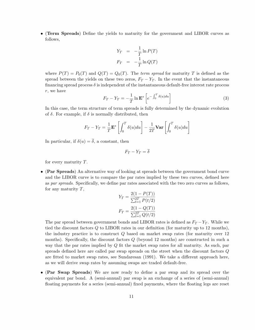
• (Term Spreads) Define the yields to maturity for the government and LIBOR curves asfollows,
YT = − 1T
lnP (T )
FT = − 1T
lnQ(T )
where P (T ) = P0(T ) and Q(T ) = Q0(T ). The term spread for maturity T is defined as thespread between the yields on these two zeros, FT − YT . In the event that the instantaneousfinancing spread process δ is independent of the instantaneous default-free interest rate processr, we have
FT − YT = − 1T
lnE∗[e−∫ T
0δ(u)du
](3)
In this case, the term structure of term spreads is fully determined by the dynamic evolutionof δ. For example, if δ is normally distributed, then
FT − YT =1T
E∗[∫ T
0δ(u)du
]− 1
2TVar
[∫ T
0δ(u)du
]
In particular, if δ(u) = δ, a constant, then
FT − YT = δ
for every maturity T .
• (Par Spreads) An alternative way of looking at spreads between the government bond curveand the LIBOR curve is to compare the par rates implied by these two curves, defined hereas par spreads. Specifically, we define par rates associated with the two zero curves as follows,for any maturity T ,
YT =2(1− P (T ))∑2Tt=1 P (t/2)
FT =2(1−Q(T ))∑2Tt=1Q(t/2)
The par spread between government bonds and LIBOR rates is defined as FT −YT . While wetied the discount factors Q to LIBOR rates in our definition (for maturity up to 12 months),the industry practice is to construct Q based on market swap rates (for maturity over 12months). Specifically, the discount factors Q (beyond 12 months) are constructed in such away that the par rates implied by Q fit the market swap rates for all maturity. As such, parspreads defined here are called par swap spreads on the street when the discount factors Qare fitted to market swap rates, see Sundaresan (1991). We take a different approach here,as we will derive swap rates by assuming swaps are traded default-free.
• (Par Swap Spreads) We are now ready to define a par swap and its spread over theequivalent par bond. A (semi-annual) par swap is an exchange of a series of (semi-annual)floating payments for a series (semi-annual) fixed payments, where the floating legs are reset
11
on a semi-annual basis. Specifically, the floating receiver receives, at the end of each paymentperiod t (t = 1, · · · , 2T ), an amount equivalent to the six-month LIBOR interest, i.e.,
1Qt/2−τ (τ)
− 1, (τ =12)
whereas the fixed-side receiver receives a fixed amount of FT2 . The notional of one dollar is
exchanged at the maturity date T . Under the assumption of no-default, the fair market fixedrate for a par swap can be determined in such a way that the market value of all floatingpayments equals to the market value of all fixed payments:
2T−1∑t=0
E∗[e−∫ t/2+τ
0r(u)du ×
(1
Qt/2(τ)− 1
)]=
2T∑t=1
FT2P (tτ)
or equvalently,
2T−1∑t=0
E∗
e− ∫ t/2
0r(u)du × e
−∫ t/2+τ
t/2r(u)du
Et/2[e−∫ t/2+τ
t/2R(u)du
]
− P (t/2 + τ)
=FT2
2T∑t=1
P (tτ) (4)
Let YT denote the yield of a government bond priced at par, then YT is Determined as
1− P (T ) =YT2
2T∑t=1
P (tτ)
or equivalently,
2T−1∑t=0
(E∗[e−∫ t/2+τ
0r(u)du
]− P (t/2 + τ)
)=YT2
2T∑t=1
P (tτ) (5)
Subtracting (5) from (4), we obtain
2T−1∑t=0
E∗
e− ∫ t/2
0r(u)du ×
Et/2[e−∫ t/2+τ
t/2r(u)du
]
Et/2[e−∫ t/2+τ
t/2R(u)du
]− 1
=
FT − YT2
2T∑t=1
P (tτ)
The left-hand-side of the equation is roughly the present value of LIBOR-repo differentials orshort-term financing spreads. Indeed, when δ is independent of r, we can simplify the aboveexpression as
2T−1∑t=0
E∗
e− ∫ t/2
0r(u)du ×
1
Et/2[e−∫ t/2+τ
t/2δ(u)du
]− 1
=
FT − YT2
2T∑t=1
P (tτ) (6)
In particular, if δ(u) = δ, a constant, then
2T−1∑t=0
E∗[e−∫ t/2
0r(u)du ×
(eδτ − 1
)]=FT − YT
2
2T∑t=1
P (tτ)
12
In summary, par swap spreads can be interpreted as the present value of the stream of short-term financing spreads, properly amortized over the swap payment period. In particular,the positive spreads of swap rates over government bond yields can be attributed entirely tothe positive spreads of LIBOR rates over GC-repo rates. Swap spreads, therefore, serve anindicator for the credit quality of banks involved in the LIBOR fixing, not the credit qualityof the counterparty involved in the swap transaction.
We point out that although the above three forms of swap-related spreads are different bydefinition, the term structures of these spreads, i.e., spreads as a function of maturity, shall sharemore or less the same shape. In other words, if term spreads are upward sloping (downward slopingor humped), then par spreads as well as par swap spreads will also be upward sloping (downwardsloping or humped).
We shall also point out that even though swaps are priced as default-free, there is strong corre-lation between corporate spreads and swap spreads. Loosely speaking, par spreads are essentiallycorporate spreads for the average banks involved in the LIBOR resetting. As such, the term struc-ture of swap spreads is highly correlated with the term structure of corporate spreads. In practice,corporate spreads are defined for a combination of financial and non-financial firms while the creditquality of the reference banks in the LIBOR basket tends to be controlled by BBA which has theoption to replace the bed names by good names. Consequently, corporate spreads are usually pricedwider than swap spreads (see Collin-Dufresne and Solnik (1999)) and are highly correlated withswap spreads.
4 Term Structures of Swap Spreads: Models
In this section we construct term structures of swap spreads using the basic analytical frameworkoutlined in the previous sections. Our eventual objective is to construct a 3-factor swap spreadmodel that would allow us to examine the impact of short-term financing spreads, liquidity premiumand risk premium on the term structure of swap spreads.4 For ease of demonstrations, we start witha simple one-factor model, i.e. the one-factor Vasicek’s model for the default-free instantaneousinterest rate as well as for the instantaneous financing spread. We show how the default-freeassumption of swaps generates the term structure of swap spreads. Next, we extend the one-factormodel to a 2-factor framework so that we can examine the level and slope of swap spread curveand explore the notion of risk premium and liquidity premium. Finally, we introduce the 3-factormodel that demonstrates how the dynamics of instantaneous financing spreads, risk premium andliquidity premium jointly determine the term structure of swap spreads.
4.1 Swap Spreads in a Single-Factor Setting
We first analyze term structures of swap spreads under the assumption of a one-factor Vasicek’smodel.5 Specifically, we assume that the default-free instantaneous interest rate process r (i.e., the
4It is well-known that three factors are necessary in order to characterize movements of default-free yield curves,see Littleman and Scheinkman (1991). Similar conclusion can be confirmed from historical swap spreads.
5The use of Guassian models suffers from the usual blame for negative interest rates and negative swap spreads.Alternatively, we may choose a one-factor Cox, Ingersoll and Ross (1985)’s model as our basic interest rate process.Our results shall not be materially different.
13
overnight GC-repo rate) and the instantaneous financing spread process δ (i.e., the overnight LIBORrate minus the overnight GC-repo rate) are determined by the following stochastic processes, seeVasicek (1977),
dr = kr(r − r)dt+ σrdwr
dδ = kδ(δ − δ)dt+ σδdwδ
where kr and kδ are (non-negative) constants for the mean-reversion of the two processes, σr andσδ (positive) constants for volatility, r and δ (positive) constants for the long-run mean, wr and wsare two independent Brownian motions under the probability measure P .6
For the purpose of pricing under no-arbitrage, we seek an equivalent martingale measure P ∗ forr and δ so that under P ∗,
w∗r = wr − λrdt, w∗δ = wδ − λδdt
become two independent Brownian motions, where λr and λδ, respectively, are the market price ofrisk or the risk premium corresponding to the risk associated with each factor. Both risk premiumparameters are usually positive. We assume for the purpose of this paper that λr and λδ areconstants. Under the equivalent martingale measure P ∗, we can write the stochastic dynamics ofr and δ as
dr = kr(r∗ − r)dt+ σrdw∗r
dδ = kδ(δ∗ − δ)dt+ σδdw∗δ
where krr∗ = krr + λrσr and kδδ∗ = kδδ + λδσδ. Note that when kr > 0, r∗ = r + λrσr/kr. Thus,the long-run mean of r under P ∗ is adjusted upward by a constant term. Moreover, the larger therisk premium of the short rate factor, λr, the larger the long term mean r∗. For example, withkr = 0.5, λr = 0.2 and σr = 0.01, the long-run mean of r is adjusted upward by about 40bp.Similar statement can be made for δ∗.
For ease of illustrations, we first consider the term structure of term spreads.
Proposition 1 The term structure of term spreads under our 1-factor setting is given by
FT − YT = ψ(kδT )δ0 + (1− ψ(kδT ))δ∗ − ηT (7)
where ψ(x) ≡ 1−e−x
x and ηT is a deterministic function of T , given by
ηT =σ2δ
2Tk2δ
∫ T
0(1− e−kδ(T−u))2du
A number of observations can be drawn from Proposition 1. The term structure of term spreadsmean-reverts to their long run mean of δ∗. An increase in the initial short-term financing spreadsincreases the level of term spreads in the short-end, and thereby flattens the term structure of termspreads. An increase in the long-run mean of the short-term financing spread increases the level of
6Historically, correlation between changes in Treasury yields and changes in swap spreads has not been found tobe either positive or negative consistently. As such, our assumption of zero correlation between wr and wδ is notunreasonable.
14
term spreads in the long-end, and thereby steepens the term structure of term spreads. When thecurrent short-term financing spread is less (or greater) than its long run mean, the term structureof term spreads is strictly upward (or downward) sloping. The larger the volatility of short-termfinancing spreads, the smaller the overall level of term spreads. However, the volatility effect isalmost negligible. For example, if σδ = 0.01, kδ = 0.45 and T = 10, the volatility contribution tothe 10yr term spread is a mere 1.5bp. Finally, the larger the risk premium λδ for δ, the larger thelong-run mean δ∗ and the steeper the term spread curve.
Figure 2 plots term structures of term spreads, par spreads and (default-free) par swap spreadsfor the following set of parameters:
Par spreads are calculated based on the discount factors used for term spreads. In calculating parswap spreads, we make use of formula (6), which implies that,
FT − YT =2∑2T
t=1 P (tτ)
2T−1∑t=0
P (tτ)∆(tτ)
where
∆(t) = E∗
1
Et[e−∫ t+τ
tδ(u)du]
− 1
Under our assumption, δ(t) is normally distributed, allowing us to derive a close form expressionfor ∆(t):
∆(t) = E∗[eτψ(kδτ)δ(t)+τ(1−ψ(kδτ))δ
∗−γ(τ) − 1]
= eτψ(kδτ)E∗[δ(t)]+ 1
2τ2ψ(kδτ)
2Var∗[δ(t)]+τ(1−ψ(kδτ))δ∗−γ(τ) − 1
where
γ(τ) =σ2
2k2δ
∫ τ
0(1− e−kδ(τ−u))2du
E∗[δ(t)] = e−kδtδ0 + (1− e−kδt)δ∗
Var∗[δ(t)] = σ2δ tψ(2kδt)
We note that in Figure 2 the term structure of term spreads and the term structure of par spreadsshare much of the same shape. This is not surprising, as it is consistent with the observation that thespot yield curve usually has the same shape as the par yield curve. Figure 3 also indicates that theterm structure of par spreads is almost exactly identical to the term structure of par swap spreads.The difference between the two, for the parameters chosen here, is less than 0.5 basis points. Thisis comforting, since it suggests that in the one-factor setting the current industry practice of fittingthe par rates implied from the LIBOR zero curve to market swap rates is practically equivalent tofitting the default-free par swap rates to market swap rates.7 Given the close relationship between
7While the difference between par spreads and par swap spreads may be larger in a multi-factor framework, theindustry practice of fitting a few key points on the curve (such as fitting the 2yr, 10yr and 30yr swap rates) controlsthe difference between par and par swap spreads at all maturities.
15
term spreads and par spreads or par swap spreads, for the rest of the paper, we will focus primarilyon the term structure of term spreads for our purposes of studying term structures of swap spreads.
It is useful to note that when the mean-reversion coefficient of the instantaneous financingspreads equals that of the default-free instantaneous interest rates (as in Figure 2), we can collapsethe two state variables into a new state variable. This allows us to characterize the term structureof swap rates using the new state variable. Specifically, letting R = r + δ, we have
dR = kR(R−R)dt+ σRdwR
where kR = kr = kδ, R = r + δ, σR =√σ2r + σ2
δ , and σRdwR = σrdwr + σδdwδ. Under thissetup, the instantaneous interest rate associated with swap rates can be equivalent modeled by asingle-factor R, which has a starting value of R0 = r0 + δ0, a long-run mean of R = r + δ under Pand a long-run mean of R∗ = r∗ + δ∗ under P ∗, implying a risk premium of
λR =λrσr + λδσδ√
σ2r + σ2
δ
In Figure 2, given the parameters for processes r and δ, we have
The usefulness of this approach will be demonstrated in the next two sub-sections when we introducemulti-factor models of swap spreads.
4.2 Swap Spreads in a 2-Factor Setting
One of the critical disadvantages of single-factor interest rate models is that these models canonly generate term structures of interest rates and term structures of swap spreads that are eitherupward sloping or downward sloping. Yield curve shifts implied by single-factor models can onlyexplain curve reshapings corresponding to either a steepening or a flattening move. It is empiricallyknown that two or three independent factors are necessary in order to characterize the dynamicbehavior of yield curve movements, e.g., Litterman and Scheinkman (1991). It is equally plausiblethat two or three factors are required to describe the dynamic behavior of swap spread movements.
In this section, we extend the single-factor swap spread model of the previous section into a2-factor framework in which the instantaneous default-free interest rates as well as the instanta-neous financing spreads are driven by two latent state variables. Specifically, we assume that theinstantaneous short-rate is given by
r = x1 + x2
where the two stochastic latent factors are described by two mean-reverting processes:
dx1 = k1(x1 − x1)dt+ σ1dw1
dx2 = k2(x2 − x2)dt+ σ2dw2
Here, k1, k2, x1, x2, σ1 and σ2 are (non-negative) constants, and w1 and w2 are two correlatedBrownian motions with Cov(dw1, dw2) = ρdt under P . With appropriately chosen parameters, we
16
can relate factor x1 to the overall interest rate level or long-term interest rate and factor x2 to theslope factor or spread between the short- and long-term interest. The sum of x1 and x2 becomes themodel-implied instantaneous short rate.8 For the purpose of pricing, we again seek the equivalentmartingale measure P ∗ so that under P ∗,
w∗1 = w1 − λ1t, w∗2 = w2 − λ2t
are two Brownian motions under P ∗ with Cov(dw∗1, dw∗2) = ρdt. The dynamics of x1 and x2 under
P ∗ become
dx1 = k1(x∗1 − x1)dt+ σ1dw∗1
dx2 = k1(x∗2 − x2)dt+ σ2dw∗2
where k1x∗1 = k1x1 + λ1σ1 and k2x
∗2 = k2x2 + λ2σ2.
Similarly, we can extend our single-factor financing spread process into a two-factor setting suchthat the process for the instantaneous financing spreads is given by
δ = δ1 + δ2
where δ1 and δ2 are two mean-reverting processes (independent of w1 and w2):
dδ1 = kδ1(δ1 − δ1)dt+ σδ1dwδ1
dδ2 = kδ2(δ2 − δ2)dt+ σδ2dwδ2
with Cov(dwδ1 , dwδ2) = ρδdt, and kδ1 , kδ2 , δ1, δ2, σδ1 and σδ2 are constants. With properly chosenparameters, δ1 can be related to the level of swap spreads, while δ2 can be interpreted as theslope of swap spreads. Together, δ1 + δ2 defines the implied swap spread in the short end or theinstantaneous financing spread. We assume that under the equivalent martingale measure P ∗,
w∗δ1 = wδ1 − λδ1t, w∗δ2 = wδ2 − λδ2t
are two Brownian motions with the same correlation structure and the dynamics of δ1 and δ2 underP ∗ become
dδ1 = kδ1(δ∗1 − δ1)dt+ σδ1dw
∗δ1
dδ2 = kδ2(δ∗2 − δ2)dt+ σδ2dw
∗δ2
where kδ1δ∗1 = kδ1δ1 + λδ1σδ1 and kδ2δ
∗2 = kδ2δ2 + λδ2σδ2 .
We present our main result on the term structure of swap spreads in the following proposition.
Proposition 2 The term structure of term spreads under our 2-factor setting is given by
FT − YT = ψ(kδ1T )δ1(0) + ψ(kδ2T )δ2(0) + (1− ψ(kδ1T ))δ∗1 + (1− ψ(kδ2T ))δ∗2 − ηT (8)8In this 2-factor setup, the factor which has a slower speed of mean-reversion corresponds typically to the level
factor; whereas the factor with a faster speed of mean-reversion is likely the slope factor.
17
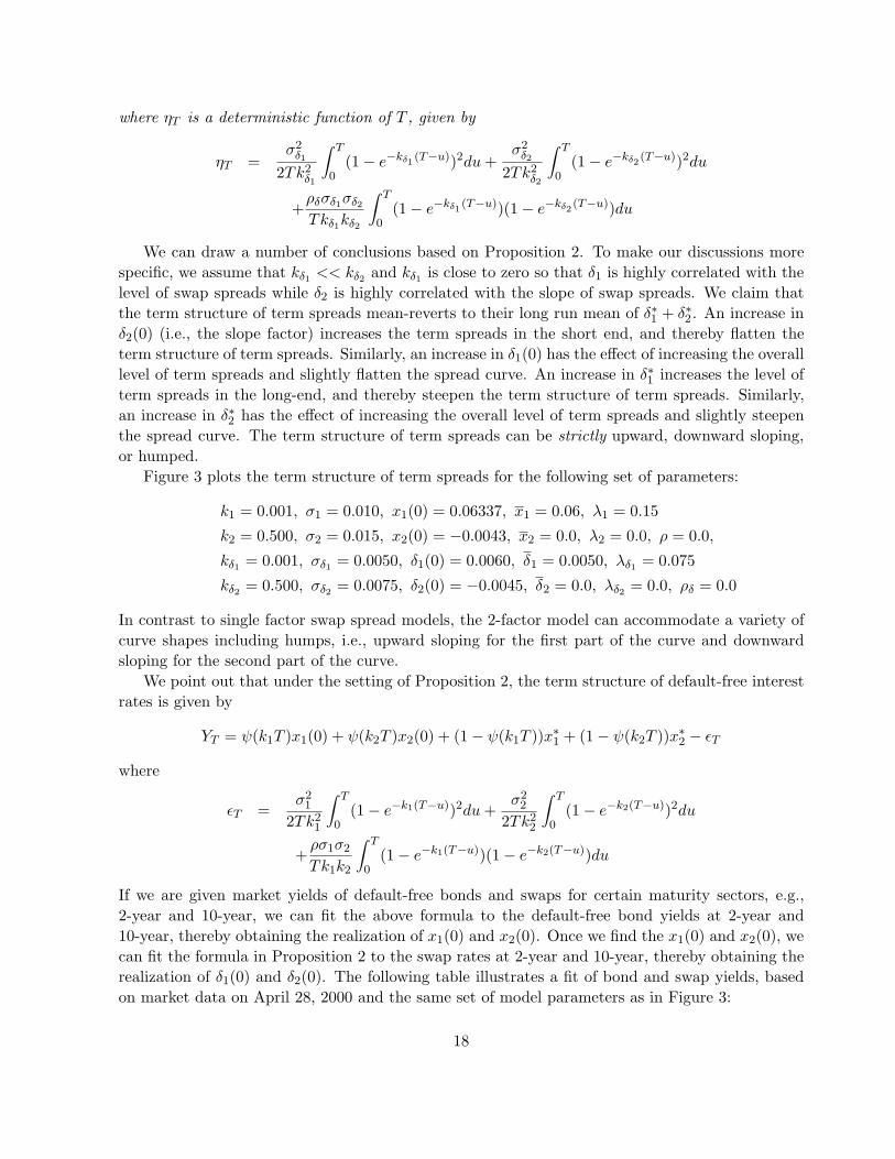
where ηT is a deterministic function of T , given by
ηT =σ2δ1
2Tk2δ1
∫ T
0(1− e−kδ1
(T−u))2du+σ2δ2
2Tk2δ2
∫ T
0(1− e−kδ2
(T−u))2du
+ρδσδ1σδ2Tkδ1kδ2
∫ T
0(1− e−kδ1
(T−u))(1− e−kδ2(T−u))du
We can draw a number of conclusions based on Proposition 2. To make our discussions morespecific, we assume that kδ1 << kδ2 and kδ1 is close to zero so that δ1 is highly correlated with thelevel of swap spreads while δ2 is highly correlated with the slope of swap spreads. We claim thatthe term structure of term spreads mean-reverts to their long run mean of δ∗1 + δ∗2 . An increase inδ2(0) (i.e., the slope factor) increases the term spreads in the short end, and thereby flatten theterm structure of term spreads. Similarly, an increase in δ1(0) has the effect of increasing the overalllevel of term spreads and slightly flatten the spread curve. An increase in δ∗1 increases the level ofterm spreads in the long-end, and thereby steepen the term structure of term spreads. Similarly,an increase in δ∗2 has the effect of increasing the overall level of term spreads and slightly steepenthe spread curve. The term structure of term spreads can be strictly upward, downward sloping,or humped.
Figure 3 plots the term structure of term spreads for the following set of parameters:
In contrast to single factor swap spread models, the 2-factor model can accommodate a variety ofcurve shapes including humps, i.e., upward sloping for the first part of the curve and downwardsloping for the second part of the curve.
We point out that under the setting of Proposition 2, the term structure of default-free interestrates is given by
If we are given market yields of default-free bonds and swaps for certain maturity sectors, e.g.,2-year and 10-year, we can fit the above formula to the default-free bond yields at 2-year and10-year, thereby obtaining the realization of x1(0) and x2(0). Once we find the x1(0) and x2(0), wecan fit the formula in Proposition 2 to the swap rates at 2-year and 10-year, thereby obtaining therealization of δ1(0) and δ2(0). The following table illustrates a fit of bond and swap yields, basedon market data on April 28, 2000 and the same set of model parameters as in Figure 3:
The starting values of the two bond factors are 5.254% and 2.034 %, respectively, implying aninstantaneous short-rate of 7.288%. The starting values of the two swap spread factors are 123.9bp and -103.3 bp, respectively, implying an instantaneous financing spread of 20.6 bp. The instan-taneous short-rate for the swap curve is 7.5%.
Similar to the single-factor case, we explore the special case when k1 = kδ1 and k2 = kδ2 . DefineX1 = x1 + δ1 and X2 = x2 + δ2. It is easily verified that
dX1 = k1(X1 −X1)dt+ σX1dwX1
dX2 = k2(X2 −X2)dt+ σX2dwX2
where X1 = x1 + δ1, X2 = x2 + δ2, σX1 =√σ2
1 + σ2δ1
and σX2 =√σ2
2 + σ2δ2
. Under the equivalentmartingale measure P ∗, we have
dX1 = k1(X∗ − x)dt+ σX1dw∗X1
dX2 = k2(Y ∗ − Y )dt+ σX2dw∗X2
where X∗1 = x∗1+δ∗1 and X∗
2 = x∗2+δ∗2. In summary, similar to our 2-factor model for the governmentcurve, we obtain a 2-factor model for the swap curve with exactly the same stochastic structure asfor bonds. For the parameters given in Figure 3, we have
The parameters in Figure 3 were chosen so that swaps and bonds can be fitted separately. We notewhen the term structure of swap spreads is upward sloping, a typical fit to bond yields and swaprates usually gives rise to δ1(0) = X1(0) − x1(0) > 0 while δ2(0) = X2(0) − x2(0) < 0. In otherwords, the implied level or long rate based on the swap curve is higher than that implied from thegovernment curve, while the implied the slope factor based on the swap curve is steeper than thatof the government curve. The processes δ1 and δ2 can be interpreted as follows.
Interpreting δ1:
δ1 represents the spread differential between long-term swap rates and long-term governmentbond yields. We argue that this spread is determined by the following two economic factors: 1)market expectations of future short-term financing spread and 2) risk premiums required for holdinglong-term bonds and long-dated swaps.9
• Market expectations of interest rates in the future affect long-term swap rates as well aslong-term bond yields. Expectations of higher rates in the future generally result in higher
9In this paper, we only study the risk premium required for the level factors x1 and X1 while ignoring the riskpremium associated with the slope factors x2 and X2.
19
long-term swap rates as well as higher long-term bond yields. However, the net effect on thelevel differential between swaps and bonds shall be negligible. However, expectations of futureshort-term financing spreads affect only the swap rates. Expectations of higher short-termfinancing spreads in the future can lead to higher long-term swap rates relative to bonds,thereby increasing the spread differential between the two level factors.
• The risk premium, also known as term premium, refers to the additional expected returnfixed-income investors demand in order to compensate for the risk of holding longer termbonds (or swaps). Bond (swap) risk premiums make long-term interest rates higher thanit would otherwise be. When fixed income investors demand more risk premium for holdinglonger term swaps than bonds of equal maturity, the long-term swap rates may be higher thanit would other wise be. The risk premium differential between swaps and bonds is affectedby the supply and the demand of government bonds vs the supply and the demand of swaps.
Interpreting δ2:
δ2 defines the slope differential between the swap curve and the bond curve. We argue thatthe slope differential characterizes the risk premium differential as well as the liquidity premiumdifferential between swaps and government bonds. Note that the slope of the term structure ofdefault-free interest rates is affected by two economic forces: 1) market expectation of future interestrates and 2) the term premium required for holding longer term bonds and the liquidity premiumcommended by government bonds (e.g., on-the-runs).
• Market expectations of interest rate movements in the near and distant future affect the slopeof the yield curve in the short and intermediate sectors. But, such effect is applicable to bothswaps and bonds. The net effect on the slope differential between the swap curve and thegovernment curve may be trivial. In other words, the slope of swap spreads shouldn’t bematerially affected by the expectations of future interest rates.
• The risk premium and liquidity premium affect the slope of yield curve in a significant way.
– Bond (swap) risk premiums make the yield curve steeper than it may otherwise be.When fixed income investors demand more risk premium for holding longer term swapsthan for holding bonds of equal maturity, the term structure of swap rates becomessteeper than that of government bond yields, especially at the long-end.
– The liquidity premium refers to the additional price investors are willing to pay for bondswith liquidity. In general, on-the-run bonds are far more liquid than swaps with equiv-alent maturity. If the 10 year on-the-runs commend more (or less) liquidity premiumthan the 2-year on-the-runs, then it may cause the bond yield curve to be flatter (orsteeper) than it would otherwise be. The liquidity deferential in bonds and swaps maycause the swap curve to be steeper (or less steeper) than the bond curve, which impliesa steeper (or flatter) term structure of swap spreads.
– It is known that a large population of fixed-income money managers are mandated toinvest a significant proportion of their assets in government bonds. In contrast, fixed-income money managers are typically forbidden from using swaps as an investment tool.
20
The natural demand for swaps comes from corporations or dealers involving in long-term financing or hedging. Globally, the 10-year sector has traditionally been the mostdemanded sector among all maturity sectors, creating additional liquidity premium forthe sector while causing the term structure of swap spreads more likely to be upwardsloping.
In summary, the level factor δ1 is affected by market expectations of financing spreads in the longrun. Both δ1 and δ2 are influenced by the risk premium and the liquidity premium.
4.3 Swap Spreads in a 3-Factor Setting
In constructing term structures of swap spreads using the 2-factor model proposed in the previoussection, we took the approach to fit bond yields and swap rates for maturities at 2-year and 10-year.Unfortunately, the instantaneous interest rates implied by fitting the 2-year and 10-year sectorsmay be ill-behaved and not consistent with the actual overnight rates observed in the market.Consequently, instantaneous finance spreads, upon which the term structure of swap spreads isconstructed, may not be consistent with the actual financing spreads observed in the market. Toresolve this problem, we extend our 2-factor model to include an additional factor which tracks thedynamic behavior of the instantaneous short rates.
Formally, we consider a 3-factor default-free term structure model under which the dynamicsof the first two factors, economic latent variables x1 and x2, is given by
dx1 = k1(x1 − x1)dt+ σ1dw1
dx2 = k2(x2 − x2)dt+ σ2dw2
where all parameters are the same as those defined in the previous section, while w1 and w2 aretwo correlated Brownian motions. As in the previous section, under suitable choice of the meanreversion parameters k1 and k2, the first factor x1 tracts movements of long-term interest rates,while the second factor x2 tracts movements of yield curve slope. Together, Θ = x1 + x2 definesthe model implied short-rate, which can be interpreted as the “equilibrium” short rate necessary toaccommodate the prevailing state of the economy. For example, if the current state of the economyis such that it is heading towards recession, then the model implied short-rate may necessitate alevel that is lower than the current market short-rate.
Alternatively, we interpret Θ as a theoretical target rate. Specifically, we model the evolution ofthe instantaneous default-free interest rate as a policy rule controlled by the central bank,
dr = kr(Θ− r)dt+ σrdwr
where kr and σr are constants, and wr is a Brownian motion independent of w1 and w2. Thatis, the instantaneous short-rate, controlled by the monetary policy authority, mean-reverts to theequilibrium target rate, subject to a random noise due possibly to transitory imbalance in themoney market.10 If the current short-term interest rate is below the equilibrium target rate, thenthere is a tendency that the central bank may hike the short-term interest rate to gradually catch
10See Piazessi (2000) for a similar specification with the central bank controlling short-term interest rates under ajump-diffusion setting.
21
up with the equilibrium short-term target rate. Similarly, if the current short-rate is higher thanthe equilibrium target rate, then it is more likely that the central bank will guide the short-rategradually down towards its equilibrium target.
For purposes of pricing securities under the no-arbitrage condition, we assume there exists anequivalent martingale measure P ∗ under which,
w∗i = wi − λit, i = 1, 2, r
are converted into standard Brownian motions. In other words, under P ∗, the dynamics of x1, x2
and r take the following form:
dx1 = [k1(x1 − x1) + λ1σ1]dt+ σ1dw∗1
dx2 = [k2(x2 − x2) + λ2σ2]dt+ σ2dw∗2
dr = [kr(Θ− r) + λrσr]dt+ σrdw∗r
Moreover, the no-arbitrage price at time t of a zero coupon bond maturing at time T can bedetermined as
Pt(T ) = E∗t
[e−∫ T
tr(s)ds
]We need the following lemma for constructing term structures of government bond yields, swaprates and swap spreads.
Lemma 1 Under the 3-factor setting specified above, the yield to maturity of default-free zerocoupon bonds has the following closed form formula:
Lemma 1 provides a complete solution to the term structure of zero coupon bonds. Specifically,given initial values of x1, x2, and r, we can generate yields to maturity for zero coupon bonds of allmaturities. Formula (9) suggests that yields to maturity are linearly related to the three interestrate factors. Under the assumption that k1 << k2 and k1 is close to zero, we can make the followingobservations. First, an increase in x1(0) increases the overall level of interest rates (especially inthe long-end) while having no material impact on the short-end of the curve. Second, an increasein x2(0) flattens the yield curve. Finally, an increase in r(0) sharply increases the short-end of thecurve while having no material impact on the long-end of the curve.
Our 3-factor model also suggests that yields to maturity are linearly related to the three riskpremium parameters, i.e., λ1, λ2 and λr. Each risk premium plays the role of steepening theyield curve for each of its relevant maturity sector. In other words, each demands additional yieldcompensation for risk bearing. In fact, it is easily shown that that for any zero coupon bond, itsexcess return can be explained by
E[dP
P
]− r = λr(σrTAT ) + λ1(σ1TBT ) + λ2(σ2TCT )
Based on the loadings of AT , BT and CT , bonds with very long maturity are primarily priced byλ1 while bonds with very short maturity are primarily priced by λr, and the intermediate sector ispriced by λ2.
Given our experience with 1- and 2-factor models, we specify the dynamics of short-term fi-nancing spreads δ using the same analytical structure. Specifically, under the probability measureP , we assume that δ is governed by the following dynamic system,
dδ1 = kδ1(δ1 − δ1)dt+ σδ1dwδ1
dδ2 = kδ2(δ2 − δ2)dt+ σδ2dwδ2
dδ = kδ(δ1 + δ2 − δ)dt+ σδdwδ
With a suitable choice of parameters, δ1 represents the overall level of swap spreads (level factor)while δ2 represents the slope of swap spread curve (slope factor). The sum of δ1 and δ2 is themodel implied short-term financing spread, i.e., the implied financing spread that is consistentwith the term structure of swap spreads in the intermediate and long maturity sectors. Finally,δ itself corresponds to the instantaneous financing spread. The 3-factor structure imposed hereallows us to capture the over-all shape of the swap spread curve, including the short-end as well asthe long-end. Moreover, we can study the dynamic behavior of the swap spread curve by trackingthe dynamic behavior of each of the three swap spread factors. For the dynamics of δ under theequivalent martingale measure P ∗, we assume that
are independent Brownian motions under P ∗, and λδ1 , λδ2 and λδ are constant parameters forrisk premiums. The following proposition constructs the term structure of term spreads using theformula derived in Lemma 1.
Proposition 3 The term structure of term spreads under our 3-factor setting is given by
FT − YT = aT δ(0) + bT δ1(0) + cT δ2(0) + dT (10)
where aT , bT , cT , and dT are the same as AT , BT , CT and DT in Lemma 1 with all parametersfor x1, x2 and r replaced by those of δ1, δ2 and δ.
Equation (10) provides the analytical formula necessary for constructing term structures ofswap spreads. However, if we make the convenient assumption that the mean-reversion parameterscorresponding to the 3-term structure factors in the swap space are identical to those of the bondspace, i.e., k1 = kδ1 , k2 = kδ2 and k3 = kδ, then we can determine swap rates in a simple 3-factorframework as well. Specifically, the 3-factor model for swaps takes the following form:
dX1 = k1(X1 −X1)dt+ σX1dwX1
dX2 = k2(X2 −X2)dt+ σX2dwX2
dR = k3(X1 +X2 −R)dt+ σRdwR
where X1, X2, σX1 , σX2 and σR are related to those parameters defining the default-free interestrate process and the short-term financing spread process as follows,
X1 = x1 + δ1, X2 = x2 + δ2
σX1 =√σ2x1
+ σ2δ1, σX2 =
√σ2x2
+ σ2δ2, σR =
√σ2r + σ2
δ
and the risk premium parameters for X1, X2 and R are determined by
λX1 =λx1σx1 + λδ1σδ1
σX1
, λX2 =λx2σx2 + λδ2σδ2
σX2
, λR =λRσR + λδRσδR
σR.
5 Term Structure of Swap Spreads: Empirical Results
In this section we turn to the empirical implementation of the 3-factor model outlined in theprevious section. Our first task is to parameterize our model. This is achieved by adopting some ofthe existing empirical work. Given the parameterization, we then fit our model to historical bondyields and swaps rates. This allows us to examine empirically the impact on swap spreads of theshort-term financing spreads, liquidity premium, and risk premium.
Our parameterization takes two steps. In the first step, following the empirical work of Duffieand Singleton (1997), Babbs and Nowman (1999), and Mendev-Vives and Naik (2000), we setk1 = 0 and k2 = 0.5, i.e., x1 follows a random walk while x2 is mean-reverting with a half-life of1.4 years. In all these three studies, the mean reversion of the first factor is near zero while themean reversion of the second factor is around 0.5. For k3, which is a parameter characterizing thecentral bank’s responsiveness to deviation from the market required short-rate, we assign it a value
24
of 1.5, implying a half-life of about 6 months.11 Similarly, we set kδ1 = 0, kδ2 = 0.5 and kδ = 1.5.Given that k1 = 0, we can assume without loss of generality that x1 = x2 = 0 and δ1 = δ2 = 0since all constant terms can be absorbed into the initial values of x1 and δ1. For specificationof the volatility parameters, we again borrow the empirical estimates from Duffie and Singleton(1997), setting σ1 = 0.009, σ2 = 0.014 and ρ = 0, which is consistent with their estimates of theinstantaneous volatility (of the square-root processes evaluated at the means).12 For σ3, we assigna value of 0.0050 or 50 basis points, which is consistent with that of Mendev-Vives and Naik (2000).For the spread volatility parameters, we set σδ1 = 0.0025, σδ2 = 0.0035, ρδ = 0 and σδ = 0.0025.This implies that σX1 = 0.009341, σX2 = 0.014431, and σR = 0.00559. Finally, for the risk premiumparameters, we assume that λ2 = λr = 0 and λδ2 = λδ3 = 0. The preliminary study by Meandev-Vives and Naik (2000) indicates that both λ2 and λr are not equal to zero, while Longstaff (2000),using a more carefully chosen proxy for the instantaneous short rates, demonstrates that the termpremium at the short-end is statistically insignificant. We choose to set these parameters to zeroas we are not confident about their true values. In setting λ2 = λr = 0, we can focus exclusivelyon the risk premium associated with holding long-term securities.
To generate our model yield curves that fit historical rates, we take as given the market yieldsfor maturities at the short-end (the instantaneous short-rate), the 2-year sector, the 10-year sectorand the long-end (the 30-year sector). While we have previously fitted x1 and x2 to rates atthe 2-year and 10-year sectors in our 2-factor framework, we now expand our fitting of r to theshort-end as well. In addition, we take the 30-year market rate as a benchmark for assessing themarket-required risk premium for holding long-term government bonds or swaps. To summarize,for each given market yield curve, we search for a risk premium parameter λ1 (or λX1) so thatthe model yield curve generated by Lemma 1 fits the market yield curve jointly at the short-end,2-year, 10-year and 30-year sectors.13
In the second step of parameterization, we modify the volatility and correlation parameters bythe sample volatilities and sample correlations corresponding to the historical factor realizationsobtained in the first step. Ideally, if the volatility and correlation parameters chosen for the firststep are true, then the sample volatilities and sample correlations implied from the historical factorsshall be reasonably close. By enforcing this second step of iteration, we can have a better chance tofind the true volatility and correlation parameters. For fitting bond yields, we re-set σ1 to 0.0125and σ2 to 0.0150 while allowing a negative correlation of -0.30 between x1 and x2. For fitting swaprates, we re-set σX1 to 0.0135 and σX2 to 0.0168 while allowing a negative correlation of -0.23between X1 and X2. Finally, we also re-set σr to 0.005 and σR to 0.0075, based on the samlpevolatility of r and R observed from the first step.
In our first step fitting, we also find that the time series of the risk premium factor is negativelycorrelated with the realized level factor for both bonds and swaps. Specifically, we regress the
11Meandev-Vives and Naik (2000) report a value of 0.82. We choose a higher numerical value based on our intuitionthat the US Federal Reserve, under the leadership of Chairman Greenspan, is aggressive and proactive when it comesto setting its monetary policy in line with macroeconomic fundamentals.
12Both Babbs and Norman (1999) and Mendev-Vives and Naik (2000) obtain much higher estimates for σ1 and σ2
due to the negative correlation between the two factors.13By fitting λx1 or λX1 for each weekly observation, we have implicitly allowed the risk premium parameter to be
time-varying, even though long-term bonds are priced with a constant risk premium parameter on a given day. Thisapproach is revised in the second step.
25
realized risk premiums against the realized level factors and find that for bonds, we have
λx1(t) = 0.2480− 2.026x1(t), R2 = 0.25
while for swaps, we have
λX1(t) = 0.2204− 1.284X1(t), R2 = 0.147
with very significant t-statistics for both regressions, -10.18 and -7.312 respectively. As a result,we impose in our second step a specification for the risk premium parameter using the above linearregression result. In doing so, the level factor for the bond curve becomes a mean-reverting processunder the equivalent martingale measure:
dx1 = (0.2480− 2.026x1 + ε)σ1dt+ σ1dw∗1
The term ε represents a small error. We will take ε as a free parameter and fit to the data.Hopefully, ε will be zero on average. The level factor for the swap curve becomes
dX1 = (0.2204− 1.284X1 + ε)σX1dt+ σX1dw∗X1
under the equivalent martingale measure.
The Data:
The data set used for our empirical study is obtained from Lehman Brothers, Inc. This dataset includes weekly observations of government bond yields and swap rates from January 1995 toDecember 2000, based on the Friday’s closes. For government bonds, the Lehman’s data includesconstant maturity treasury (CMT) rates for maturities of 2-year, 10-year and 30-year, for both theon-the-run and off-the-run bonds. The off-the-run yields are calculated as the constant maturitytreasury (CMT) rates obtained by smoothing the off-the-run bond yields. We note that the yieldspreads between the off-the-runs and on-the-runs provide us an unusual time series of specialnessfor the on-the-run bonds. The Lehman’s data set also includes mid-market constant maturity swap(CMS) rates for maturities of 2-year, 10-year and 30-year. Combining our data for bonds andswaps, we can derive a time series of swap spreads associated with the on-the-run as well as theoff-the-run bonds.
As an independent check on the data, we compare the Lehman data with Bloomberg whichprovides historical data for both government yields and swap rates. The two sources of data aregenerally consistent, although Bloomberg lacks historical data for the off-the-run bond yields andthe 30-year swap rates. For short-term interest rates, we obtain the repo rates for general collateralfrom Lehman while the 1-month LIBOR rates are downloaded from Bloomberg. We note thatour data set covers several economic and business cycles in which the Federal Reserve have botheased and tightened monetary policy. Except for the Mexico crisis in 1995, the first half the samplerepresents rather calm and normal economic environment. However, the second half of the samplecovers several extraordinary events including the crisis of LTCM in the Fall 1998, the liquidity crisisof Y2K in the Summer 1999, and the Treasury buyback in the Spring 2000.
26
Results:
Table 1 presents summary statistics for the three interest rate factors (i.e., the short-rate factor,the long-rate factor, and the slope factor) and the risk premium factor (associated with the long-ratefactor), based on fitting the GC-repo rates and the off-the-run treasury yields at the 2-year, 10-year,and 30-year sectors and on fitting the 1-month LIBOR rates, and swap rates at the 2-year, 10-year,and 30-year sectors. Table 1 also reports summary statistics for the spreads between the swapfactors and bond factors, i.e., swap factors minus bond factors. Table 2 examines the correlationstructure and volatility for the three bond factors and the three swap factors, and reports thesample correlation coefficients (off diagonal) and sample annualized volatilities (diagonal) of theweekly changes in these factors. Figures 4(a)-(d) plot the time-series history of the three interestrate factors and the risk premium factor associated with the long-rate factor, based on fitting thebond yields and the swap rates, and the time-series of the spread between these two histories offactors.
Volatilities and Correlations:
Table 2 reveals that the first differences or changes of the three bond factors are at best weaklycorrelated. The highest correlation coefficient is -0.342 (between the long-rate factor and the slopefactor), i.e., higher long rates are more likely to be associated with a steeper yield curve. Thiscoefficient matches our model correlation parameter of -0.30. Our assumption of zero correlationbetween the short-rate and long-rate factors and between the short-rate and slope factors is rea-sonably close to their sample correlations. Our assumption of volatilities (0.0125 for x1, 0.0150 forx2, and 0.005 for r) also matches those of the sample volatilities (0.0132 for x1, 0.0153 for x2, and0.0045 for r). For swaps, the sample correlation between the long-rate factor and the slope factoris -0.2586, which again matches our model assumption of -0.23. However, the volatility assumptionof 0.135 for X1 is slightly larger than its sample volatility of 0.0129, while the volatility assumptionof 0.0165 for X2 and 0.0075 for R is largely in line with the sample volatilities. We also examinethe correlation between the risk premium factor and the level factor. For both bonds and swaps,we find that the correlation between the risk premium factor and the level factor is near zero.Regressing the risk premium factor against the level factor results in insignificant t-statistics.
We note that given our parameterized volatility and correlation coefficients for the bond andswap factors, we can back out the implied model assumption for the spread process δ. Indeed, itcan be easily shown that the volatilities implied by our assumptions on the bond and swap factorsimply that σδ1 = 0.0050 and σδ2 = 0.0070 and σδ = 0.0055. Unfortunately, these numbers areslightly off from their sample volatilities (0.0061 for σδ1 , 0.0120 for σδ2 and 0.0079 for σδ). Themodel correlation between δ1 and δ2 implied by our assumption for x and X is around -0.2, which issignificantly below its sample correlation of -0.849. Table 2 suggests that when swap spreads widen,the term structure of swap spreads tends to steepen and that the swap spread in the short-end isnot very correlated with the swap spread in the long-end. Altogether, we conclude that our modelmay still be slightly mis-specified.
Short-Rate and Long-Rate Factors:
Table 1 and Figures 4(a),(b) show that the short-rate and long-rate factors corresponding to
27
swap rates are usually higher than those factors corresponding to government bond yields, with amean difference of 19.5 and 30.9 basis points, respectively. The mean short-rate difference representsan average of short-term financing spreads, while the mean long-rate difference represents an averageof long-term term spreads (or swap spreads). While the short-rate differences have been wellbehaved, fluctuating narrowly around its mean of 20 basis points (except for periods near the endof calendar year, known as the term effect), the long-rate differences have been steadily risingfrom around 20-30 basis points in 1995-1997 to near 110 basis point by late 2000. Clearly, this isrelated to the fact that long-term swap spreads have been steadily rising and reached their historicalwides in the Spring 2000. The long-rate differentials peaked in the Fall 1998, the Summer 1999and the Spring 2000. The correlation between the long-rate spread and the short-rate spread isaround 0.25, implying a weak positive relationship between long-term swap spreads and short-termfinancing spreads.
For a brief period in early 1995 and late 1999, the long-rates implied by the swap curve fallsbelow those of the bond curve. This happened at the time when the term structure of swap spreadswas flat or near inverted.
Model-Implied Short-Rates:
The sum of the mean long-rate difference and the mean slope difference is about 44 basis points.This sum can be interpreted as the model-implied short-term financing spread, which may serveas the near-term target towards which the current short-term financing spread will converge. Themodel-implied financing spreads have been steadily rising during the period covered in our sample,from around 20 basis points in early 1998 to over 100 basis points in early 2000. In other words,based on the market prices in 2000, the US bond market was expecting the short-term financingspread to become much higher in the future. This is consistent with the view that bonds will becomemore special in the future as the US government continues to reduce the supply of Treasury bonds.
Slope Factors:
Over the sample period considered here, the slope factor corresponding to swap rates is slightlylarger than that of bond yields, with a mean difference of 13.3 basis points. In other words, theyield curve corresponding to the off-the-run bonds is slightly steeper than that of swaps so thaton average, the term structure of swap spreads (up to the 10-year maturity) is near flat or slightlydownward sloping. However, the slope differential between swaps and bonds reached its low of-92.88 basis points in late 1998 in the aftermath of the LTCM crisis. The slope of the swap curvewas much steeper than that of the bond curve so that the term structure of swap spreads becameextremely upward sloping. The slope differential between the swap curve and the bond curvereached its local low level of near 0 basis point in the summer of 1999 when Y2K was a big concern,and -45 basis points in the Spring of 2000 when Treasury announced its buyback. The swap spreadcurve was also very steep in December 1995 when the slope differential reached -60 basis points.
We point out that the term structure of swap spreads would become much steeper had we fittedthe bond yields using the on-the-runs (instead of the off-the-runs). In particular, the mean slopedifferential between the swap curve and the bond curve would be negative, implying an upwardsloping term structure of swap spreads on average. The slope would slide even further towards itslow during the periods of LTCK crisis in 1998, Y2K liquidity crisis in 1999 and Treasury buyback
28
in 2000.
Risk Premium and Swap Spreads:
On average, the risk premium required by long-dated swaps is about 2.38% higher than that oflong-term bonds. Figure 4(d) demonstrates that during the 1998 financial crisis, the risk premiumsimplied from the long-dated swaps and long-term bonds exploded to a high around 19-20%. Therisk premium difference between the two curves dropped to -3.26% during that period. In otherwords, relative to long-dated swaps, the market was demanding a much higher risk premium forholding long-term government bonds. We note that during that time, the term structure of swapspreads had a humped shaped (upward sloping from 0 to 10-year and downward sloping from 10to 30-year). This happened because long-term bonds (such as those of 30-year’s) became lessattractive relative to intermediate-term bonds (such as those of 10-year’s) and the risk premiumrequired by the swap market is much less than that required by the bond market. However, theterm structure of swap spreads became strictly increasing since late 1999, especially since early2000 after US Treasury Department announced its first-ever Treasury Buy-back program in recenthistory. The risk premium implied from bonds dropped from its peak of 20% in 1998 to a low of4-5% in the beginning of 2000. The risk premium demanded for holding long-term bonds droppedsignificantly due to the strong demand for long-term government bonds (especially the 20-year plussector). In the mean time, the risk premium associated with long-dated swaps reached a levelaround 8-9%, and the risk premium differential between swaps and bonds peaked to 7-8%. Thesign change in the risk premium differential is the main reason why the term structure of swapspreads has become strictly upward sloping (even beyond 10-year) since the beginning of 2000.
Liquidity Premium and Swap Spreads:
We now take a closer look at the relationship between the liquidity premium associated withgovernment bonds and the term structure of swap spreads. First, we point out that in general theliquidity premium is hard to quantify. Specifically, we don’t have a variable that is observable yetprovides a direct measurement for liquidity premium. Second, liquidity premium can affect thepricing of all government bonds relative swaps, widening or narrowing the overall spread betweenswaps and government bonds. Liquidity premium can also affect a specific sector of governmentbonds so that it may steepen or flatten the term structure of swap spreads. Third, the yield spreadsbetween the on-the-run and off-the-run bonds serve a good indicator of the excess demand for theon-the-run bonds over the supply, and can therefore be used as a proxy for assessing the liquiditypremium commended by government bonds. In other words, when the on-the-run bonds are inspecial and traded rich, there is a good chance that this sector of bonds is priced with liquiditypremium. As such, it can put pressure on the swap spreads of this sector.
Figure 5 plots the time-series of yield spreads between the on-the-run and off-the-run bonds.The plot shows a clear widening in spreads between the off-the-run and on-the-run bonds, whichcoincides with the overall widening of swap spreads since 1998. The average on/off-the-run spreadsare 3 basis points for the 2-year sector, 14.8 for the 10-year sector and 9.8 basis points for the30-year sector. If we split the sample into two parts: pre-December 1997 and post-January 1998.Then, we find that prior to 1998, the on/off-the run spreads were 1.5 basis points for 2-year, 7.6basis points for 10-year and 4.8 basis point for 30-year. However, since 1998, the on/off-the run
29
spreads have increased drastically, averaging 4.6 basis points for 2-year, 21.9 basis points for 10-year, and 14.7 basis point for 30-year. Clearly, the 10-year sector has gained the most, relatively.This is consistent with the fact that the term structure of swap spreads has been steepenning eversince the LTCM crisis. As the 10-year bonds trade rich and commend more liquidity premium,the 10-year sector exhibits the widest swap spread, making the term structure of swap spreadssteeper from the 2-year to 10-year. Note the brief drop of specialness in late 1999 coincided withthe flattenning of the swap spread curve in late 1999.
6 Summary
In this paper we present a new approach of analyzing term structures of swap spreads using thenotions of short-term financing spreads, liquidity premium and risk premium. Our approach departsfrom the traditional approach of attributing swap spreads to counterparty risk of default. Wepresent an empirical analysis of swap spreads using data from the US market. Using our 3-factorterm structure model as lenses and filters, we are able to explain some of the extreme movementsin US swap markets in recent years. In particular, recent market data from bonds and swapssuggest that the financial market is rationally anticipating rising short-term financing spreads,rising liquidity premiums for holding government bonds, and lowering required risk premiums forholding long-term government bonds, as the expected US government surpluses may reduce the netsupply of the government bonds in the future. The empirical results reported in the paper shallprovide useful insights for both academic researchers and industry practitioners.
30
ReferenceBrown, Keith, W. Harlow, and Donald. Smith, 1994, An empirical analysis of interest rate swap
spreads, Journal of Fixed Income March, 61-78.
Babbs, Simon and K. Nowman, 1999, Kalman filtering of generalized Vasicek term struture models,Journal of Financial and Quantitative Analysis 34, 115-131.
Black, Fisher and John Cox, 1976, Valuing corporate securities: Some effects of bond indentureprovisions, Journal of Finance 31, 351-367.
Chen, Andrew and Arthur Selender, 1994, Determination of swap spreads: An empirical analysis,working paper, Southern Methodist University, 1994
Collin-Dufresne, Pierre and Bruno Solnik, 1999, On the term structure of default premia in theswap and LIBOR markets, working paper, Carnegie Mellon University.
Cooper, Ian, and Antonio Mello, 1991, The default risk of swaps, Journal of Finance 46, 597-620.
Cox, John, Jonathan Ingersoll and Stephen Ross, 1985, A theory of the term structure of interestrates,” Econometrica 53, 385-407.
Duffie, Darrell, and Ming Huang, 1996, Swap rates and credit quality, Journal of Finance 51,921-949.
Duffie, Darrell, and Kenneth Singleton, 1997, An econometric model of the term structure ofinterest rate swap yields, Journal of Finance 52, 1287-1321.
Duffie, Darrell, and Kenneth Singleton, 1999, Modeling term structure of defaultable bonds, Re-
view of Financial Studies 12, 687-720.
Das, Sanjay, and Peter Tufano, 1996, Pricing credit-sensitive debt when interest rates, creditRatings and credit spreads are stochastic, Journal of Financial Engineering 5, 161-198.
Evans, E. and G. Bales, 1991, What drives interest rate swap spreads?, in Interest Rate Swaps,Carl Beidleman, ed., 280-303.
Grinblatt, Mark, 1999, An analytical solution for interest rate swap spreads, forthcoming in Reivew
of International Finance.
Harrison, Michael, and David Kreps, 1979, Martingale and multiperiod securities markets, Journal
of Economic Theory 20, 381-408.
Jarrow, Robert, and Stuart Turnbull, 1995, Pricing derivatives on financial securities subject todefault risk, Journal of Finance 50, 53-85.
Jarrow, Robert, David Lando, and Stuart Turnbull, 1997, A Markov model for the term structureof credit spreads, Review of Financial Studies 10, 481-523.
Leland, Hayne, 1994, Corporate debt value, bond covenants, and optimal capital structure, Journal
of Finance 49, 1213-1252.
31
Leland, Hayne and Klaus Toft, 1995, Optimal capital structure, endogenous, bankruptcy, and theterm structure of credit spreads, Journal of Finance 51, 987-1019.
Litterman, Robert and Jose Scheinkman, 1991, Common factors affecting bond returns, Journal
of Fixed Income 1, 51-61.
Litzenberger, Robert, 1992, Swaps: plain and fanciful, Journal of Finance 47, 831-850.
Longstaff, Francis and Eduardo Schwartz, 1995, A simple approach to valuing risky fixed andfloating rate model, Journal of Finance 50, 789-821.
Longstaff, Francis, 2000, The term structure of very short-term rates: New evidence for theexpectations hypothesis, Journal of Financial Economics 58, 397-415.
Madan, D., and H. Unal, 1994, Pricing the risks of default, working paper, University of Maryland.
Mendez-Vives, D., and V. Naik, 2000, The economic factor model: Theory and uses, workingpaper, Fixed Income Research, Lehman Brothers, Inc.
Merton, Robert, 1974, On the pricing of corporate debt: The risk structure of interest rates,Journal of Finance 29, 449-470.
Minton, B., 1993, An empirical examination of U.S. dollar swap spreads, working paper, Universityof Chicago.
Nielsen, Soren and Ehud Ronn, 1997, The valuation of default risk in corporate bonds and interestrate swaps, Advances in Futures and Options Research, 9, 175-196.
Piazzesi, Monika., 2000, An econometric model of the yield curve with macroeconomic jumpeffects, working paper, Stanford University.
Sorensen, Eric and Thierry Bollier, 1994, Pricing swap default risk, Financial Analyst Journal,May-June, 23-33.
Sun, Tong-Sheng, Suresh Sundaresan, and Ching Wang, 1993, Interest rate swaps: An empiricalinvestigation, Journal of Financial Economics 34, 77-99.
Sundaresan, Suresh, 1991, Valuation of swaps, in Recent Developments in International Banking
and Finance, S. Khoury, ed., Amsterdam: North Holland.
Vasicek, Oldrich, 1977, An equilibrium characterization of the term structure, Journal of Financial
Mean 5.5573 5.2588 0.2585 0.1248Bonds Stdev 0.5928 0.7240 0.5476 0.0351
Maximum 6.5554 6.6263 1.5779 0.1951Minimum 4.7215 3.5690 -1.2246 0.0461
Mean 0.2346 0.4590 0.1872 0.0266Spreads Stdev 0.1881 0.3234 0.4065 0.0236
Maximum 1.3042 1.1441 1.5236 0.0816Minimum -0.0597 -0.2627 -0.9288 -0.0326
Summary statistics of yield curve factors based on fitting the weekly off-the-run government bond yieldsand the weekly swap rates. The sample period is 1995:1-2000:12.
Annualized volatility (diagonal) and correlation coefficients (off-diagonal) for weekly changes of yieldcurve factors based on fitting the weekly on-the-run government bond yields and the weekly swap rates. Thesample period is 1995:1-2000:12.