i

Erasmus University Rotterdam

MSc in Maritime Economics and Logistics

2014/2015

Modeling the entrepreneurial investment decision in the containership segment: Second hand boxship

purchase or placement of an order for a new build? The case of Panamax and Post-Panamax

containerships

by

Andreas Katsinas

Copyright © Andreas Katsinas

ii

Acknowledgments

In this section I would like to express my great appreciation and gratitude to all the individuals – friends and colleagues - who kindly and beneficially assisted the drawing of this master thesis. Special reference should be attributed to my supervisor Mr. Bart Van Riessen who offered me exceptional guidance through valuable and constructive suggestions from the beginning of this paper throughout the conclusions. The dedication of Mr. Riessen to spend his valuable time so generously has led substantially to the upcoming results, for which I am awfully proud. Furthermore, a credit of a few lines should be dedicated to my family that supported me wholeheartedly at full length of this demanding and stressful year. It will never be forgotten. Finally, I would like to dedicate the last sentence of the acknowledgements to all the members of the faculty of Maritime Economics and Logistics who did their best, in all aspects, to assist students and provide a professional but welcoming environment that hosted our dreams and ambitions. ‘Health is the greatest gift, contentment the greatest wealth, faithfulness the best relationship.” L.B. Blessings.

iii

Abstract Shipping industry, and consequently liner shipping, is governed by a well-witnessed volatility that pervades on shipping investments. Especially after the booming years from 2003 and onwards, and the steep slump that followed, the market became extremely competitive and unstable. Some would say that the increased volatility of the market creates the attractiveness of the sector for investors as high risks usually bring along high yields. Nevertheless, there are several impacting determinants and cornerstones that need to be taken into consideration beforehand, from existing or new coming investors, who aim to rush into the excitement of investing in liner shipping industry. This study aims to quantify, based on quantitative analysis using the Eviews 8 software, the initial entrepreneurial investment decision in the containership segment: Second hand boxship purchase or placement of an order for a new build, specifically for the Panamax and Post-Panamax container vessels, after presenting a brief market research on the liner shipping industry. According to our opinion, as introduced initially for the tanker sector by Merikas (2008), what matters is not the second hand price and its determinants per se, but instead of this approach we constructed the functional relationship between second hand price over the new building price and its main determinants in the container sector. By following this path we can treat our dependent variable (Second-Hand Prices / New Building Prices) as; a useful tool for the initial investment decision between a second-hand containership and a newbuilding, and second of all as a mechanism for estimating the value of the asset for financial purposes. For the purpose of the research we gathered time series of raw data (prices of 5-year-old containerships, prices of newbuildings, Libor interest rates that represent a measure of entrance in the containership sector or further expansion, time charter rates for 1 year contracts, and the respective transaction volume) for the time period between 2002 and 2011. By applying the Maximum Likelihood Estimation we can imprint the parameters estimation for the variance equation, while the application of GARCH (1,1) will allow us to capture the volatility of the dependent variable (SHP/NBP), and consequently the risk proxy by the variance. Overall we can claim that the cyclical nature of the shipping industry, together with the expectations of the actors is substantially impacting on the movement of the ratio. A low SHP/NBP ratio depicts that ship owners see a growing market in the near future and can afford to wait for another two or three years until the delivery of the new vessel based on the assumption that the freight rate is not currently peaking, and vice versa.

iv

Table of contents

i. Acknowledgements…………………………………………………………. ii ii. Abstract………………………………………………………………………..iii iii. List of tables…………………………………………………………………..vii iv. List of figures………………………………………………………………….ix

v. List of abbreviations……………………………………………………..x

Chapter 1 Introduction 1.1 Background……………………………………………………………………...1

1.1.1 The shipping industry- a brief introduction……………………………….1 1.1.2 The liner shipping industry…………………………………………………1

1.2 Scope……………………………………………………………………………..2 1.3 Objective………………………………………………………………………….5 1.4 Research question………………………………………………………………6 1.5 Thesis structure………………………………………………………………….6

Chapter 2 Market research and Literature review

2.1 Globalization and global trade…………………………………………………8 2.2 The importance of developing economies…………………………………..11 2.3 Global economic recession and its impacts on shipping investments……13 2.4 The evolution of containerization……………………………………………..13 2.5 The trend of gigantism of container vessels grows and impacts………….16 2.6 Transport costs in liner shipping and economies of scale…………………18 2.7 The shipping cycle and the perceived risk of shipping investments………20 2.8 Liner shipping as a capital market and problem identification……………..22 2.9 Literature review-previous studies linked to the investigated topic………..24

2.9.1 Ship prices…………………………………………………………………...26 2.9.2 Modeling/ Autoregressive models and techniques……………..……….27 2.9.3 Price determinants………………………………………………………….30 Chapter 3 The decisions facing shipowners, and the critical dilemma

between second hand and new build containership

3.1 The decisions facing shipowners and the four shipping markets…………..30 3.1.1 the sale and purchase market……………………………………………...32 3.1.1 the newbuilding market……………………………………………………..33

3.2 The S&P and newbuilding contracts…………………………………………..34 3.3 Sale/purchase with employment……………………………………………….35 3.4 The dilemma between second hand and new building vessel and identification of the main determinants affecting this initial investment decision……….……….36 3.5 How can we create a decision making tool for this critical investment decision?...........................................................................................................38

Chapter 4 Research methodology and data

4.1 Identification of the dependent variable………………………………39 4.2 Identification of the independent variables…………………………...39 4.3 Building the functional relationship between second hand prices over the newbuilding prices and its main determinants in the segment- the general model presentation………………………………………………….……….41

v

4.4 Model variations………………………………………………………...42

Chapter 5 Results and data analysis 5.1 Data………………………………………………………………....44

5.1.1 Problems experienced with data……………………………..44 5.1.2 Classification of containerships in terms of capacity……....45

5.2 Panamax results…………………………………………………..45 5.2.1 Key findings of the research for Panamax vessels…..........48

5.3 Post-Panamax results………………………………………….…49 5.3.1 Key findings of the research for Post-Panamax vessels….50

Chapter 6 Conclusions

6.1 Conclusions………………………………………………………..51 6.2 Recommendation for further research……………………….…51

Bibliography…………………………………………………………...53 Appendices………………………………………………………….…56

APPENDIX A Panamax ADF Test for the first differences of GDP………………………….56 ADF Test for the first differences of inflation………………………56 ADF Test for the first differences of Libor………………………….57 ADF Test for the first differences of the ratio SHP/NBP…………57 ADF Test for the first differences of time charter rates…………..58 ADF Test for the first differences of the transaction volume…….58 ADF Test for GDP……………………………………………………59 ADF Test for inflation………………………………………………..59 ADF Test for Libor……………………………………………………60 ADF Test for the ratio SHP/NBP……………………………………60 ADF Test for time charter rates……………………………………..61 ADF Test for transaction volume……………………………………61 Post-Panamax ADF Test for the first differences of the ratio SHP/NBP…………62 ADF Test for the first differences of time charter rates…………..62 ADF Test for the ratio SHP/NBP……………………………………63 ADF Test for time charter rates………………………………….....63 ADF Test for transaction volume…………………………………...63 APPENDIX B Panamax Graphs

vi

First differences of GDP……………………………………….….64 First differences of inflation…………………………………….…64 First differences of Libor…………………………………………..65 First differences of the ratio SHP/NBP…………………………..65 First differences of time charter rates……………………………66 First differences of transaction volume………………….……….66 Of GDP………………………………………………………………67 Of inflation…………………………………………………………...67 Of Libor………………………………………………………….…...68 Of time charter rates…………………………………………….....68 Of transaction volume……………………………………………...69 Post-Panamax graphs First differences of the ratio SHP/NBP……………………….….69 First differences of time charter rates……………………………70 First differences of transaction volume………………………….70

Of the ratio SHP/NBP……………………………………………..71 Of time charter rates………………………………………………71 Of transaction volume…………………………………………….72 APPENDIX C Panamax GARCH model variation 1……………………………………….73 GARCH model variation 2……………………………………….74 GARCH model variation 3……………………………………….75 Post-Panamax GARCH model variation 1………………………………………..76 GARCH model variation 2………………………………………..77 GARCH model variation 3………………………………………..78 APPENDIX D Panamax Correlogram model 1……………………………………………..79 Correlogram model 2……………………………………………..80 Correlogram model 3……………………………………………..81 ARCH LM test for model 1……………………………………….82 ARCH LM test for model 2……………………………………….83 ARCH LM test for model 3……………………………………….84 Histogram- Normality test for model 1………………………….84 Histogram- Normality test for model 2………………………….85 Histogram- Normality test for model 3………………………….85

vii

Post-Panamax Correlogram model 1……………………………………………….86 Correlogram model 2……………………………………………….87 Correlogram model 3……………………………………………….88 ARCH LM test for model 1…………………………………………89 ARCH LM test for model 2…………………………………………90 ARCH LM test for model 3…………………………………………91 Histogram- Normality test for model 1……………………………91 Histogram- Normality test for model 2……………………………92 Histogram- Normality test for model 3……………………………92

APPENDIX E Memorandum of agreement (all 6 pages)……………………….93

viii

List of tables

Table 1: Total containership fleet by size sector- by No. of units…………….....3 Table 2: GDP and merchandise trade by region, 2011-13………………………10 Table 3: The containerization degree (in %) in a number of EU ports………….14 Table 4: World container slot capacity by ship size 1982-1998…………………19 Table 5: Summary of ADF stationarity test for all variables…………………...…43 Table 6: General model and model variations……………………………………..46 Table 7: Summary of residual diagnostics for all model variations for Panamax

vessels……………………………………………………………………….52 Table 8: Summarized results of Akaike Information Criterion for Panamax

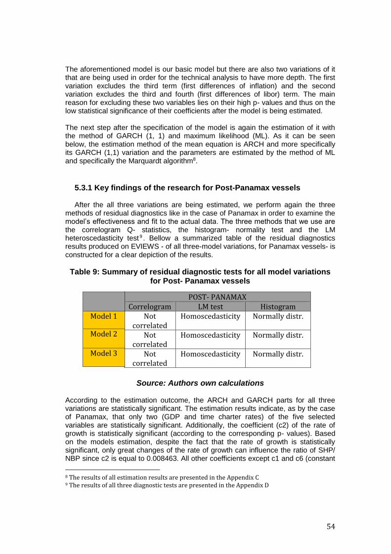
vessels……………………………………………………………………….53 Table 9: Summary of residual diagnostics for all model variations for Post-Panamax

vessels………………………………………………………………………54

ix

List of figures

Figure 1: Major seaborne trades by commodity growth rates……………………….9 Figure 2: Growth in volume of world merchandise exports and GDP, 2005-13…..11 Figure 3: The increasing significance of developing countries in world economy..12 Figure 4: Distribution of container volumes worldwide, 2015……………………….16 Figure 5: Total containership fleet by size sector- by No. of units………………….18 Figure 6: Containership deliveries+ orderbook by size- in TEU…………………….18 Figure 7: The largest containerships of the world…………………………………....20 Figure 8: The typical course of a shipping cycle……………………………………...22 Figure 9: The four shipping markets that control shipping and how they interact..33 Figure 10: Shipowner’s capital investment decision procedure…………………….40 Figure 11: Container time-charter index and the demand for capacity, 1999-09…41 Figure 12: ARCH- GARCH (1, 1) process in EVIEWS………………………………50 Figure 13: MLE process in EVIEWS…………………………………………………..51

x

List of abbreviations

SHP Second Hand Prices NBP Newbuilding Prices ARMA Autoregressive Moving Average GARCH Generalized Autoregressive Conditional Heteroscedasticity ARCH Autoregressive Conditional Heteroscedasticity CHARMA Conditional Heteroscedastic ARIMA model EGARCH Exponential Generalized Autoregressive Conditional Heteroscedasticity MLE Maximum Likelihood Estimation VAR Vector Autoregression ConRo Container Roll-On Roll-Off TEU Twenty-foot Equivalent Unit M&A Mergers and acquisitions ADF Augmented Dickey-Fuller GDP Gross Domestic Product WTO World Trade Organization GATT General Agreements on Tariffs and Trade WB World Bank E.U. European Union U.S. United States U.K. United Kingdom IMF International Monetary Fund WWII World War two UNESCAP United Nations Economic and Social Commission for Asia and Pacific ULCS Ultra Large Containerships VLCC Ultra Large Crude Carriers LOA Length overall S&P Sale and Purchase VALES Valemax Size Bulk Carriers CAPES Capesized Bulk Carriers FFA Forward Freight Agreement CP Charter-party BIMCO Baltic and International Maritime Council BDI Baltic Dry Index NSF Norwegian Sales Form MOA Memorandum of Agreement EFT Electronic Funds Transfer LC Letter of Credit SS Steam Ship

MV Motor Vessel

1

Chapter 1- Introduction

1.1 Background Shipping is admittedly one of the most fascinating business sectors, and since the first cargo was carried by sea, more than 5,000 years ago, shipping has been at the forefront of global development (Stopford 2009). The history reveals that sea transportation was the core of economic development. According to the very well-know economist of the 17th century Adam Smith, the key to evolve a capitalistic society is the division of labor. In Chapter 3 of the economic book called “The Wealth of Nations”, Adam Smith argues that while productivity increases significantly and therefore businesses produce more and more, local markets are not sufficient to cover the supply and a wider sales network could provide access to wider markets. The shipping industry can be considered as the forefront of the world trade, facilitating access to wider markets when local demand is insufficient. This chapter is structured to provide the reader with a brief background of the shipping industry. In the first sub-sections we are presenting the definition of shipping, we identify the main characteristics and differences of the shipping sub-markets while focusing particularly in the liner shipping industry. A concise throwback in history is performed to depict how the industry evolved during the past decades and which trends prevailed after all and what proved to be the main determinants of the market. Examining the history of shipping is not the core of this research but quoting Winston Churchill “the further backward I look, the further forward I can see” can reveal the truth regarding the importance of understanding the past for a successful future. Additionally, this chapter targets to give a precise idea about the scope and the objective of the study, as well as, the last sub-section illustrates the structure of the study in the following chapters. 1.1.1 the shipping industry- a brief introduction Shipping in general can be characterized as an industry with a very wide range of determinants impacting on it. There are different sub-markets, substantially inter-correlated, and that results into heterogeneous economy of the shipping sector. Shipping economics, are directly influenced by the cargo, the type of the ship, the geographical locations, and the requirements of the trade routes. Shipping can be thought as a simple industry with a clear purpose; the provision of transportation of passengers and cargoes, but in reality things is way more complicated than the aforementioned perception. In the 2nd edition of his book, Maritime Economics, Stopford (1997), provides us with a very enlightening definition of the shipping industry. “Shipping is a complex industry an the conditions which govern its operations in one sector do not necessarily apply to another; it might even, for some purposes, be better regarded as a group of related industries. Its main assets, the ships themselves, vary widely in size and type; they provide the whole range of services for a variety of goods, whether over shorter or longer distances. Although one can, for analytical purposes, usefully isolate sectors of the industry providing particular types of service, there is usually some interchange at the margin which cannot be ignored.” (Stopford 1997) This definition is pretty very much revealing regarding the shipping world. Commercial operations and economic operations must be separated and treated with different approaches and scopes. For instance, significant differences exist concerning the type of the cargo that is carried. Liner carriers focus only on deep-sea

2

transportation of general cargo (finished and semi-finished goods), while bulk carriers focus on bulk cargo (dry and liquid). Additionally, there is also a completely different economic and finance structure between those two major segments. However, it is important to realize that shipping should be treated as a single market given the fact that any company owns and operates vessels in both segments (liner and bulk) or may own and operate vessels designed for multi-purposes (i.e. ConRO ships), and therefore, shipping sector should be considered as one entity and not a group of segregated sub-markets and sub-sectors (Panagiotis 2014). The technological advancements in shipbuilding and communications provided a fertile ground for a new and more sophisticated shipping industry. Developments in ship design and construction, mainly the enlargement of the vessels and their increased efficiency, gave rose to the economies of scale, which in their turn facilitated the growth of the seaborne trade (Haralambides 2007). Trade grew significantly and consequently the operational part of transportation became way more complex and demanding. Stopford (2009), illustrates that the shipping market gradually reformed into three major segments; passenger liners, cargo liners, and tramp shipping. Passengers where considered to be the “cream” cargo and passenger liners aim to provide fast, reliable, and frequent transport on the busiest routes across the Atlantic ocean and the Far-East. Cargo liners on the other hand are very similar to passenger liners despite the fact that the carrying capacity of the vessel is filled with cargo and not passengers. Cargo liners are operating under regular schedules and are usually liken with busses, as they both provide regular, stable, frequent, and reliable pre-scheduled services. In principle, those type of vessels performing pre-scheduled routes, are equipped with several decks that provide the flexibility to charge and discharge cargo in many different ports. Finally, tramp shipping refers to the transportation of bulk cargoes (coal, grains, iron ore, oil, and oil products, etc.) on a voyage bases (Stopford 2009). While bulk shipping modeling only focuses on estimating the demand and supply functions as well as freight rate forecasting - based on the fact that the industry operates mainly on the spot market -, in liner shipping the situation is significantly differentiated. Liner shipping industry is built on the foundation of providing regular services between several ports (Haralambides 2004). In general, according to Haralambides (2007), the liner services are in principle open to anyone with cargo to be carried, and in this sense resembles to the public transport service. Furthermore, being able to provide such services on a global coverage requires a very extensive utilization of infrastructure - mainly referring to terminals/ports, cargo handling equipment, vessels, and agencies (Haralambides 2007). An illustrating example of how capital intensive the liner shipping industry is, is the one provided by the later mentioned author whom argues that a weekly service in a busy trade route such as Europe and South East Asia demands a fleet of 9 vessels deployed, amounting for more than one billion US dollars of investment. 1.1.2 the liner shipping industry Cargo carried by liner shipping companies has been characterized as general cargo. Until the 1960’s, that kind of cargo was loaded on board in many various form of packaging, namely pallets, boxes, barrels, and crates, mainly by relatively small to average size vessels, known as general cargo purpose vessels (Haralambides 2007). When the deep-sea transportation service is properly organized and operates efficiently, substantial financial benefits may occur for traditionally strong, as well as developing, trading countries. “A “healthy” and well-performing liner shipping system provides the facilities for countries to fully extract the rents related to the international trade by administering cargo owners of high-value manufactured and agricultural

3

goods with streamlined access to a ready supply of ocean transport services.” (Fusillo 2006) When trying to analyze and identify the dominating trends in liner shipping, first thing that come in mind nowadays is the enlargement of the size of the firms and the emergence of global carriers. The market share of the top ten biggest carriers-in terms of carrying capacity- grew substantially from 50% in January 2000 to 60% in January 2007, reflecting a growth in the aggregated capacity from 2,5 million TEUs in 2000, to 6,3 million TEUs in 2007 (Cariou 2008). According to the latter mentioned author, during the same period, the total market share of the five largest carriers increased form 33% to 43% respectively. Since that year there have been witnessed tremendous leaps in the shipbuilding industry that proved wrong the predictions that argued that containerships are about to reach their maximum size around 8,000 TEUs. Nowadays the global containership fleet accounts for 4.765 units of containerships, with sizes varying as follows:

Table 1: Total containership fleet by size sector- by No. of units

Capacity Range in TEUs

500-900

1000-1999

2000-3499

3500-4999

5000-7999

8000-11999

12000+

No. Of Units

685 1.233 792 771 615 471 198

Percentage of global Fleet

14% 26% 17% 16% 13% 10% 4%

Source: Banchero Costa research (Ross shipbrokers internship) The majority of the leading carriers in terms of market share quickly adopted the trend of the growing capacity of containerships in order to benefit from the occurring economies of scale though the reduction of the cost of transportation per TEU. However, it important to stress out at this point that there are several paths that liner shipping companies could choose form in order to reap the aforementioned benefits. In general, according to Cariou (2008), two main paths can be distinguished. First of all the internal (or organic) growth refers to chartering and direct capital investments in new built and second hand vessels. On the other hand, we can identify the external growth, which is mainly vectored through Mergers and Acquisitions (M&As) and strategic alliances (Cariou 2008). It is common sense, that according to the individual ship owner and the timing, one way over another is preferred; this can be justified by external factors impacting such as market conditions, financial requirements, and market power (Cariou 2008). Maersk Line for example, a leading carrier in terms of capacity and market innovation, during the past 15 years simultaneously with direct investments (second hand and new built vessels), has also been involved in several strategic alliances. Maersk initial teamed-up with SeaLand (1995-1999) right before entering into a series of M&As such as those of, Safemarine, CMB_T, and P&O and Nedlloyd in 2005 (Cariou 2008). In this way Maersk Line met an incredible external growth with significant financial results that gave the firm the competitive advantage even in times of strong economic downturns. Internal growth on the other hand was achieved for Maersk Line through direct capital investments. While discussing direct capital investments we talk about either buying a newbuilding vessel directly form the

4

shipyard, or purchasing a second hand vessel from the sale and purchase market. An additional option for reducing the amount of capital invested is chartering a vessel instead of buying a new one or a second hand vessel. The largest carriers according to Cariou (2008) are choosing to diversify their investment portfolio with both owned and chartered vessels. Maersk Line charters around 55% of its fleet while MSC and CMA (number two and number three respectively in the rankings of the Top-10 ocean carriers in terms of fleet size) chartered 40% and 65% of their fleet respectively in January 2007 (Cariou 2008). Even though the merchant ship is recognized worldwide as a real asset, and consequently shipping as a real asset’s market, the majority studies so far have examined this relationship only from the demand side (volume of transactions and price variability). The market of second hand ships and new buildings play a very critical role in the competitiveness of the shipping industry (Merikas 2008). Since the vessel is considered a real asset, especially in the second hand market substantial profit opportunities arise as investors can literally buy low and sell high. Such types of transactions are characterized as “asset play” (Merikas 2008). When investors are facing the decision whether they should dispose capital for a new build vessel or one that is already available for purchase in the second hand market, many determinants and empirical and technical criteria should be considered in advance. The most crucial factor of all is the timing of entering or exiting the market because of the cyclicality feature of the market (Merikas 2008). As illustrated by a ship owner’s testimony cited by (Stopford 2009), “when I wake up in the morning and freight rates are high, I feel good. When the are low I feel bad”, it is easily understandable that market cycles pervade the shipping world. Stopford (2009), stresses out that as the weather rules the lives of seafarers in exactly the same way market cycles waves are rippling through the financial well being of shipowners. Besides the significance of the market cycles with respect to shipping investments there other equally important and influential determinants on supply and demand. On the supply side, we have the world fleet, the fleet’s productivity, shipbuilding production, scrapping and losses, and freight revenue (Stopford 2009). On the demand side, we can identify according to the author the world economy in the first place, the seaborne commodity trades, the average haul, the random shocks, and finally the transport costs. This paper attempts to build a functional relationship with respect to the second hand price over the new building price and its most impacting determinants on the container segment, as introduced initially by the finance professor of the University of Piraeus, Andreas Merikas, in his research titled “Modeling the investment decision of the entrepreneurial in the tanker sector: Second hand Purchase or Newbuilding?” The latter study focuses on the investigation of the preceding in different ship sizes (Suezmax, Aframax, Handysize) in the tanker sector while our study aims to apply this methodology – with some small variations - for the first time in the containership segment and specifically for the Panamax and Post-Panamax containerships. By adopting this approach of research conducted in the tanker sector and applying it with the respective adjustments that will be discussed bellow, for the Panamax and Post-Panamax sizes of containerships, we can treat the dependent variable we chose, which is the ratio of the second hand price over the new building price (SHP/NBP) as:

a) A useful and easily applicable tool for the initial investment decision of the entrepreneur when facing the dilemma between second hand vessel and new built vessel, and

5

b) As a mechanism for evaluating the value of the vessel for financial purposes The aim of the paper is to investigate, for the first time in the container segment, what impacts and finally determines the variability in the ratio second-hand price of containerships over the new building price. Given the cyclical feature of the shipping industry (boom, recession, and depression) – which is explained in details in section 2.7 - and consequently the importance of the timing and the type of investments, providing a useful tool to determine the initial decision between send-hand and new built vessel, as well as a tool that can be utilized for evaluating the value of the asset, could be of a great benefit for all parties involved.

1.2 Scope of the research The sale and purchase market along with the new building market and their determinants have always been tempting sub-markets for researchers to dive into. The critical dilemma of investors whether they should purchase a newbuilding containership or a second hand vessel from the sale and purchase market is also an aspect that can be of a particular interest for actors involved in the aforementioned type of transactions. This study aims to model this initial investment decision and consequently provide a valid decision-making tool that can depict the most favorable option depending on the market conditions (independent variables). However, all studies are analyzing the relationship only from the demand side. In other words the examined relationship is the one between volume of transactions in the market (second-hand or new building) and the price of the ships. By defining as a dependent variable the ratio between second prices (SHP) over the new building prices (NBP), (SHP/NBP), we are able to provide a more accurate and complete tool for investors and shipbrokers as the modeling results acknowledge both the demand and the supply side expressed as the ratio of the first over the latter. Furthermore, only one study has been conducted by (Merikas 2008) in the past, aiming to model the critical investment decision of the entrepreneurial in the tanker sector; whether he should buy a vessel from the second-hand market or to order a new built vessel from the shipyard. This is the first attempt to model this initial decision in the container segment for the ship sizes of Panamax and Post-Panamax. There are several determinants while looking at both sides (supply and demand), identified in the research of Merikas (2008) such as the prices of the assets in the new building market, the prices of the assets in the second-hand market, the interest rates offered by shipping financial institutions for investments, the transaction volume, as well as last but definitely not least the charter rates of the vessels. Additionally, based on the relevant literature review and our estimations, we included in our model building the variables referring to GDP only of OECD countries, as well as, the inflation from year to year. The reasoning behind the adoption of all the preceding is properly explained and justified in the section regarding the research methodology and data of the study (Chapter 4).

This study is structured in a way that is easily understood even by an inexperienced reader. We decided to provide a background of the liner shipping industry (Chapter 2 and Chapter 3) before introducing the research methodology and diving into the quantitative part of the thesis. Chapter 2 is providing a brief introduction referring to the impacting forces on the shipping industry as well as presenting the most significant trends that shape the industry nowadays (sections 2.1-2.6). During the remaining sections of the chapter (2.7-2.9) we provide the reader with a good taste of the significance of the shipping

6

cycle and its relation with shipping investments, we identify the problem that pervades the segment, and finally we provide relevant information extracted from studies of other researchers that will help us through our research. Chapter 3 on the other hand is closely related to shipping investments. The chapter clearly targets to administer to the reader a clear depiction of the choices of shipowners when considering the purchase of vessel. The second hand (S&P) and new building market is presented, as well as the sale and purchase contracts of a vessel and some additional options regarding special terms of a sale and purchase contracts. Finally, this chapter is the vestibule of the core of the research that follows in chapters 4 to 6, and therefore the dilemma between second hand and new building vessel as well as the identification of the main determinants affecting this investment decision are illustrated.

1.3 Objective The purpose of this thesis is to create an investment decision-making tool when the investor is facing the classic dilemma between a second-hand purchase from the sale and purchase market and a new building purchase from the shipyard focusing on the Panamax and Post-Panamax containerships. The model produced can provide the reader great insights referring to the question of whether the investor should choose a second-hand vessel or a new built containership, as well as, will provide a mechanism for evaluating the asset’s value for future financing purposes.

1.4 Research question “Second hand boxship purchase or new build container vessel? The case of Panamax and Post-Panamax containerships” This thesis targets to model the initial investment decision of the entrepreneur in the container segment: Second hand purchase or new build containership, focusing on Panamax and Post Panamax boxships. The approach will be based on;

Market research to identify market dynamics, predominant trends, and the nature of investments in the liner shipping industry

Classification of containerships (Panamax and Post-Panamax categories are included)

Identification of the independent variables

Identification of the dependent variable

Building the model (mean equation and variance equation)

Model estimation ADF test Estimation of the mean equation with Maximum Likelihood Estimation

(MLE) Estimation of the variance equation with GARCH (1,1) model with three

kinds of error distribution (Gaussian, Student-t and GED) in order to capture the volatility of the dependent variable and consequently the risk proxy by the variance

All the results will be interpreted and presented in the corresponding chapters.

7

1.5 Thesis structure The remaining part of the thesis is structured as follows. Chapter 2: Market research and literature review This chapter aims to present a market research regarding the containership segment and examine the related literature. The chapter is divided in two parts whereas the first part presents the past and current global economic situation and how it impacts on global trade, the growth of containerization, the significance of the developing countries, as well as some dominant trends of the liner shipping directly influencing shipping investments. The second part of the chapter refers to the problem identification and the related literature review to the topic under investigation. Chapter 3: The decisions facing the shipowners, and the critical dilemma between second hand and new build containership The main target of this chapter to provide the reader with understandable information regarding the decisions investors is called to deal with in the shipping industry, as well as an overview of how those sub-markets function. In the concluding parts of the chapter, the dilemma between second-hand and new building vessel purchase is analyzed in terms of significance. Chapter 4: Research methodology and data Chapter 4 is the backbone of the thesis, as the methodology used will be discussed. The methodological approach will be presented in details as well as the software characteristics and the statistical and econometric models that were implemented to obtain the results. In this section of the study we will identify our dependent and independent variables and after that we will be able to construct the functional relationship we aim to study. Chapter 5: Results and data analysis In Chapter 5 a detailed description of the data set chosen will be performed, followed by the preliminary statistical analysis based on the aforementioned data sets. Additionally, we aim to provide the reader with an analysis of the results obtained always with respect to the research question. Chapter 6: Conclusions This chapter will consist of discussions and conclusions. We will provide a summary report of the research performed and answer the main research question. Additionally, limitations for the research, problems faced regarding the data set, unexpected findings, as well as suggestion for further research will complete the picture.

8

Chapter 2- Market research in liner shipping and Literature review

During the past decades containerization has increased importance and is the main cause of significant changes in the global structure of manufacturing production (Midoro 2005). The share of the world’s output according to the author is increasing constantly as a result of the shift of the offshore production zones in countries with low-cost operations such as China, India, South-East Asia, Eastern Europe and Central America. Consequently, manufacturers reallocated their production de-centrally in order to reap the benefits deriving from economies of scale and local structural advantages in operational costs (Midoro 2005). The increased penetration of containerization in the global trade, and consequently in seaborne trade (approximately 66% of international maritime trade), resulted into the emergence of the liner shipping industry. Containerized general cargo is nowadays transported worldwide by specialized ocean going merchant vessels managed by liner shipping companies offering frequent and reliable sailing schedules with a round-the-world geographical coverage. Additionally, liner shipping investments performance- as well as the expectations of the actors involved and consequently their actions- are closely related to extrinsic and intrinsic determinants such as: the global economy, the growth of global trade, the shipping cycle, the emergence of global alliances, the gigantism of containerships, etc. Therefore, this chapter aims to provide a brief market research regarding the significance of the aforementioned determinants and their relationship with liner shipping investments, as well as to present the identification of the problem under investigation. Furthermore, some dominant trends of the liner shipping directly influencing shipping investments are illustrated. The riskiness of shipping investments is analyzed within the framework of the shipping cycle. This informational background is essential in order to perceive the rationale and the key components for successful shipping investments while riding the wave of the shipping cycle. Additionally, this chapter will provide information regarding efforts of other researchers from the past, which conducted econometric analysis in the shipping industry with respect to shipping investments, and provided helpful and guiding material for this research.

2.1 Economic globalization and global trade

World trade includes mainly commodities traded and services. Economic globalization could be translated, despite the lack of a favorable definition, as the interdependence of the world economies derived from the increasing cross-border trade of commodities and services, the flow of international capital and the technological advancement and spread (Shangquan 2000). The author characterizes economic globalization as an irreversible trend based on the fact that market frontiers are mutually integrated and expanded worldwide. Bordo et al., (2003) identified economic globalization as the international integration in commodity, labor markets, and capital flow (Eichengreen 2003). The world has witnessed at least two episodes of globalization since the mid-19th century if markets’ integration is used as a benchmark (Baldwin 1999). According to the World Trade Report of 2008 by World Trade Organization (WTO), increased integration in trade, capital flows, and repositioning of labor are the main

9

characteristics of the most two recent episodes of globalization. However, the magnitude of contribution of each characteristic varies significantly. The advance of science and technologies has resulted to a dramatic decrease of transportation and communication costs, providing fertile ground for the flowering of economic globalization. Nowadays, ocean shipping costs amount to only half of the costs back in 1930. Same situation with airfreight (1/6 relatively to the base year mentioned above), and telecommunication costs (1% relatively to the base year mentioned above). This type of “type and space compression effect” driven by the technological advancement has resulted in dramatic reduction of international trade and investment costs (Shangquan 2000). Furthermore, institutional drivers contributed significantly to the dominance of this trend. Under the framework of two powerful regulators, GATT and WTO, a significant portion of tariff and non-tariff barriers were abolished, while many countries opened up their current accounts and capital accounts. GATT is the abbreviation for General Agreement on Tariffs and Trade according to which, the purpose was “the substantial reduction of tariffs and other trade barriers and the elimination of preferences, n a reciprocal and mutually advantageous basis”. The original GATT text is still nowadays in effect under the World Trade Organization (WTO) framework (World Trade Organization 2015). All those aspects facilitated greatly the emergence of this trend (Shangquan 2000). Trade, in particular seaborne trade, and investments to facilitate the demands grew hand by hand.

Figure 1: Major seaborne trades by commodity growth rates

Source: (Stopford 2009)

10

If we take a look at the economic statistics of the year 2013, we can identify the steep decline in economic indexes worldwide. The slow pace of trade growth can be explained by several factors, which may or may not be inter-correlated, including, the mature economy of the EU, the low import demand in developed economies (-0,3 per cent), as well as the mild import growth in developing economies (4,7 per cent) (World Trade Organization 2014). According to the WTO’s World Trade Report of 2014, the current economic slowdown, combined with the high unemployment rates in the euro area economies can justify the decline of world trade growth on 2013. Additionally, the high uncertainty regarding the timing of the Federal Reserve’s scale down of its monetary policy increases the pressure. The estimated growth of 2,2 percent concerning world trade growth in 2013 refers to the averaged volumes of merchandise imports and exports, adjusted to the individual inflation and exchange rates of each country. For the second year in a row world trade grew approximately at the same rate as the World Gross Domestic Product (GDP), rather than twice as much as the latter, which is the normally the case (World Trade Organization 2014).

Table 2: GDP and merchandise trade by region, 2011-13

GDP EXPORTS IMPORTS

2011 2012 2013 2011 2012 2013 2011 2012 2013

World 2.8 2.3 2.2 5.5 2.4 2.5 5.3 2.1 1.9

United States 1.8 2.8 1.9 7.3 3.8 2.6 3.8 2.8 0.8

South and central America

4.5 2.7 3.0 6.8 0.7 1.4 13.0 2.3 3.1

Europe 1.9 -0.1 0.3 5.6 0.8 1.5 3.2 -1.8 -0.5

EU (28) 1.7 -0.3 0.1 5.8 0.4 1.7 2.8 -1.9 -0.9

Commonwealth of independent States (CIS)

4.9 3.5 2.0 1.6 0.9 0.8 17.3 6.8 -1.3

Africa 1.1 5.7 3.8 -8.2 6.5 -2.4 5.1 12.9 4.1

China 7.7 7.7 7.5 8.8 6.2 7.7 8.8 3.6 9.9

Japan 1.4 1.6 1.5 -0.6 -1.0 -1.9 4.3 3.8 0.5

India 3.2 4.4 5.4 15.0 0.2 7.4 9.7 6.8 -3.0

Newly industrialized economies (4)

4.1 1.8 2.7 7.7 1.4 3.5 2.7 1.4 3.4

Memo: Developed eco

1.5 1.3 1.1 5.2 1.1 1.5 3.4 0.0 -0.3

Memo: Developing eco and CIS

5.7 4.5 4.4 5.8 3.8 3.6 8.0 5.1 4.7

Source: WTO World Trade Organization Report 2014

For the year 2014 economic data for the first quarter revealed a prolonged sluggishness of world trade and economic activity in developed countries despite

11

the positively translated indicators. United States reached negative (-2,1 percent) numbers regarding GDP figures, however unemployment fell bellow 6,4 percent in April. European Union witnessed its output growing by 1,3 percent, a figure analysts of Market Economics stress out that indicates the fastest growth for the last three years, mainly driven by the strong activity in Germany and the United Kingdom. Asia on the other hand started to grow with a constantly increasing tempo. Japan’s GDP grew substantially with an annualized increase of 5,9 percent, while China seems like turning around the negative economic indicators of 2013 (World Trade Organization 2014).

Figure2: Growth in volume of world merchandise exports and GDP, 2005-13

Source: WTO World Trade Report 2014

2.2 The importance of developing economies In general, the developing countries’ economic opportunities lie heavily on the industrialized economy. Nevertheless, the share of world output, and capital flows that can be attributed to developing countries presents substantial increase during the past decades. In this sense, “reverse linkages” between developing and industrial countries deserve our attention (Ghosh 1996). According to the IMF’s (International Monetary Fund) report produced by Ghosh (1996), “… as trade between developing and industrial countries grows and cross-boarder capital mobility increases, the developing countries will have a greater impact on the global economy. Although public debate has focused on possible adverse effects on the industrial economies, analysis suggests that the latter will benefit from growing

12

integration.” Nowadays developing countries represent 30 percent of world’s exports, an increase of 19,5 percent since 1996. The importance of developing countries as one of the driving sources of import demand has increased dramatically, manifests the growth of foreign exchange availability and purchasing power, as well as a tremendous appetite for imported goods and services. Particularly the imports to China from the EU increased dramatically reflecting a six times rise within a decade (1996-2006), while with the rest of the world tripled. Developing countries also imported approximately 38 percent of total U.S. exports in 2006, another important contribution to the global trade growth. On the other hand, developing countries are expected to become a significant export market in the near future. China is expected to import from U.S. and E.U. around 3,1 percent of the world’s total in 2050. Concluding, as the share and the significance of developing countries constantly increases, the share of those economies involved in world trade will increase. Economically strong China and India equals strong demand, which consequently raises expectations for transportation demand.

Figure 3: The increasing significance of developing countries in world economy

Source: World Bank data and staff estimates. (Ghosh 1996)

*Excludes the Baltic countries, Russia and the other countries of the former Soviet Union, and Central and Eastern Europe.

13

The report provided by the United Nations Conference on Trade and Development reveals another aspect of the subject, which strengthens the claim that developing countries are becoming a strong driver behind global economic growth, merchandize trade, and a vital demand factor for maritime transport. Furthermore, increased specialization in the supply side of maritime transport services facilitated higher gains of market share for developing countries in maritime business (United Nations 2013). In terms of supply in the shipping business shipbuilding, ship recycling, ship registration, ship ownership, and seafarer supply should be included. In each one of those sub-sectors developing countries increase year by year its contribution. As far as shipbuilding is concerned, almost 39 percent of the total gross tonnage delivered in 2011 was constructed in Chinese shipyards followed by Korea (35 percent), Japan (19 percent), and Philippines (1,6 percent). The majority of dry bulkers were built in China while Korea dominated at the container shipbuilding market whit a market share of 55 percent (United Nations 2013). Ship recycling was mainly geared in India (33 percent of gross tonnage recycled in 2011), and Pakistan (22,4 percent) and Pakistan (13 percent) (United Nations 2013). On the demand side, ship registration and ownership statistics depict the contribution of developing countries in maritime business. A typical merchant ship serving international trade route can literally be built, manned, operated, owned, operated, and registered in different countries. Between the leading 35 ship-owning economies, 17 were Asian established, 14 belonged in the EU, and only 4 were located in the United States (United Nations 2013). According to United Nations report (2013), in 2012, the top 20 liner operators deployed approximately 70 of the total container fleet capacity. The three leading firms are located in EU, while Asia-based companies flood the remaining top 10.

2.3 Global economic recession and its impacts on shipping investments The shipping industry took a great hit from the current prolonged economic recession that began back at 2007. The global credit crisis has hurt severely all segments of the transportation industry as demand for sea born merchant transportation derives from the performance of world trade. When world trade declines, as is the case nowadays, demand for sea born transportation is expected to move towards the same direction as the degree of correlation between them is considered to be high. The forecasts by the WTO and the World Bank predicted one of the most severe economic recessions since WWII (World War two) based on the decline of global exports by 9 percent in 2009 (World Trade Organization 2009). Furthermore, a 9 percent decrease in total economic output was projected, indicating the first decline of this indicator since 1982 (The World Bank 2009). Shipping benefits derived from the economic globalization, appear to be greater than any other sector. However, this significant interdependency makes shipping more vulnerable to economic shocks. Shipping is also vulnerable to financial meltdowns due to another profound reason. As almost every industry of increasing returns to scale, shipping bases its operation heavily on the bank credit and the financial system in general (Samaras 2010).

14

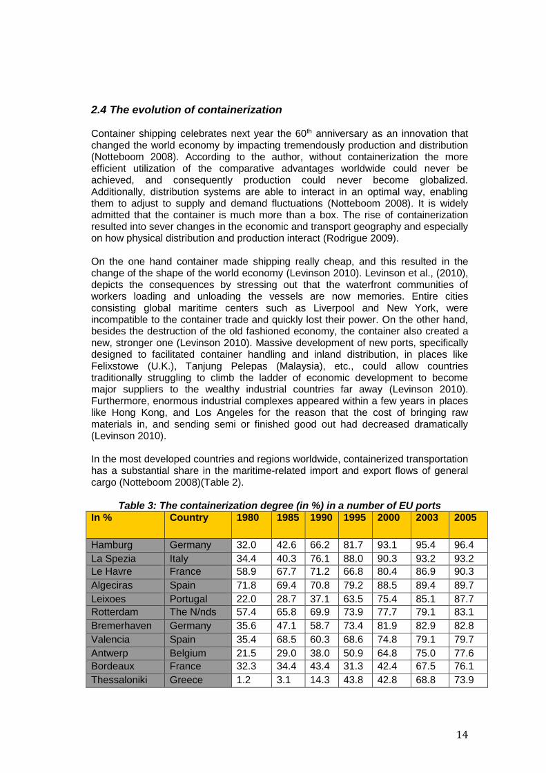
2.4 The evolution of containerization Container shipping celebrates next year the 60th anniversary as an innovation that changed the world economy by impacting tremendously production and distribution (Notteboom 2008). According to the author, without containerization the more efficient utilization of the comparative advantages worldwide could never be achieved, and consequently production could never become globalized. Additionally, distribution systems are able to interact in an optimal way, enabling them to adjust to supply and demand fluctuations (Notteboom 2008). It is widely admitted that the container is much more than a box. The rise of containerization resulted into sever changes in the economic and transport geography and especially on how physical distribution and production interact (Rodrigue 2009). On the one hand container made shipping really cheap, and this resulted in the change of the shape of the world economy (Levinson 2010). Levinson et al., (2010), depicts the consequences by stressing out that the waterfront communities of workers loading and unloading the vessels are now memories. Entire cities consisting global maritime centers such as Liverpool and New York, were incompatible to the container trade and quickly lost their power. On the other hand, besides the destruction of the old fashioned economy, the container also created a new, stronger one (Levinson 2010). Massive development of new ports, specifically designed to facilitated container handling and inland distribution, in places like Felixstowe (U.K.), Tanjung Pelepas (Malaysia), etc., could allow countries traditionally struggling to climb the ladder of economic development to become major suppliers to the wealthy industrial countries far away (Levinson 2010). Furthermore, enormous industrial complexes appeared within a few years in places like Hong Kong, and Los Angeles for the reason that the cost of bringing raw materials in, and sending semi or finished good out had decreased dramatically (Levinson 2010). In the most developed countries and regions worldwide, containerized transportation has a substantial share in the maritime-related import and export flows of general cargo (Notteboom 2008)(Table 2).

Table 3: The containerization degree (in %) in a number of EU ports

In % Country 1980 1985 1990 1995 2000 2003 2005

Hamburg Germany 32.0 42.6 66.2 81.7 93.1 95.4 96.4

La Spezia Italy 34.4 40.3 76.1 88.0 90.3 93.2 93.2

Le Havre France 58.9 67.7 71.2 66.8 80.4 86.9 90.3

Algeciras Spain 71.8 69.4 70.8 79.2 88.5 89.4 89.7

Leixoes Portugal 22.0 28.7 37.1 63.5 75.4 85.1 87.7

Rotterdam The N/nds 57.4 65.8 69.9 73.9 77.7 79.1 83.1

Bremerhaven Germany 35.6 47.1 58.7 73.4 81.9 82.9 82.8

Valencia Spain 35.4 68.5 60.3 68.6 74.8 79.1 79.7

Antwerp Belgium 21.5 29.0 38.0 50.9 64.8 75.0 77.6

Bordeaux France 32.3 34.4 43.4 31.3 42.4 67.5 76.1

Thessaloniki Greece 1.2 3.1 14.3 43.8 42.8 68.8 73.9

15

Barcelona Spain 30.0 61.3 71.0 74.3 73.9 73.4 73.1

Lisbon Portugal 32.2 47.3 58.0 65.8 69.5 72.9 72.0

Piraeus Greece 20.4 36.5 45.8 65.3 74.8 76.3 68.6

Genoa Italy 36.5 46.0 45.2 49.7 65.0 61.7 63.0

Bilbao Spain 26.4 33.0 53.1 46.7 49.2 58.1 58.9

Marseilles France 32.3 42.4 50.5 46.9 53.2 54.2 56.9

Zeebrugge Belgium 30.6 22.5 23.3 30.0 41.5 51.0 55.0

Rouen France 23.1 40.4 36.7 31.8 32.9 36.5 42.0

Amsterdam The N/nds 21.0 21.6 30.2 40.5 25.9 22.9 29.7

Trieste Italy 34.4 46.7 55.4 28.9 27.4 18.8 29.6

Dunkirk France 14.6 14.7 10.5 11.5 27.9 13.9 15.0

Zeeland Seaports

The N/nds 11.1 10.0 4.4 3.1 2.3 4.3 4.3

Source: (Notteboom 2008)

*Calculations based on data of the respective port authorities **Degree of containerization is expressed as the share of containerized cargo in

total general cargo handled in the port in terms of units of TEUs According to the report of the Economic and Social Commission for Asia and the Pacific (UNESCAP) (2005), the total volume of full containers shipped on international routes all over the world (excluding transshipment figures) accounted for 77,8 million TEU for the year 2002, compared to the figure of 28,7 million in 1990 (UNESCAP 2005). The same report provided more recently, in 2009, by UNESCAP, reveals that the expected number of containers to be shipped internationally will reach the figure of 177,6 million TEU by 2015, indicating a slower rate per annum (approximately 6,6 per cent), compared to the previous years (2002 and bellow, when the average growth had reach a rate of 8,5 per cent per annum) (UNESCAP 2009). As far as the geographical distribution of container volumes is concerned, the UNESCAP (2009) report clearly mentions that there are indications that the contributions by region in container volumes are expected to change in the near future. By 2002 East Asia had the largest part of distribution of containers accounting for 24,1 percent of the total number, followed by the EU (21,8 per cent), the North America (16,6 per cent), and the South-East Asia region (10,1 per cent) (UNESCAP 2009). However, for 2015 the report forecasts significant shifts in container distribution. East Asia is expected to grow in a faster pace than the world average, particularly due to China’s contribution, while South Asia is expected to continue with a solid growth (UNESCAP 2009). Together, Asia’s share is projected to reach 64 per cent by 2015 compared to 55 per cent in 2002. At the same time EU is slowing down substantially mainly attributing this to the maturity of its economy.

16

Figure 4: Distribution of container volumes worldwide- 2015

Source: (UNESCAP 2009)

The emergence of global liner carries was the result of the constantly changing environment of the world economy. Mindoro (2005), stresses out the fact that a few years ago the world economy was characterized by big distances, long times of services, tension in politics, and different cultures, all of them opposing strong barriers for trade. However, what is in play nowadays is a scenario of de-regulated trade through increasing geographical coverage and integration of the markets (Midoro 2005). Liner shipping witnessed significant growth rates over the past 15 years, with the worldwide container traffic increasing in a fast pace. From 30 million TEU in 1990, to 100 million TEU in 2006, and forecasts for 2020 pointed clearly at a reach of more 200 million TEU (Cariou 2008). This growth according to the researcher can be attributed to the high growth of containerization, as well as to the globalization of the world economy that led to the reallocation of the industrial production (Cariou 2008). It is common sense that in order to respond to this rapid growth liner shipping companies had to adjust their strategies, implement new ones, and innovate in order to remain competitive in terms of geographic coverage, frequency of services, supply chain management, transit times, turnaround times, and provision of value added services (Midoro 2005), (Cariou 2008). Therefore, the industry for years now is facing new challenges and structural changes reflecting on demand and supply. As far as the demand side is concerned, shippers have increased and more

17

complex demands while inducing globalization, while on the supply side, a destructive flood of overcapacity (Midoro 2005).

2.5 The trend of growing the carrying capacity of container vessels grows and impacts The rapid growth of the size of containerships is an expanding trend in liner shipping markets. Despite the fact that for the specific period 1984-1995 the maximum containership size remained stable, from that stage onwards, the maximum containership size is on the rise (Cullinane 2000). The average size shifted from 2,000 TEUs in 1995 to 3,000 TEUs in 2005, while the maximum size in operation in 1990 was 4,400 TEU compared to vessels delivered in the year 2008 that had reached a carrying capacity of more than 14,300 TEU (Cariou 2008). Nowadays, approximately 4 percent of the global container fleet amounts for containership vessels with a carrying capacity of 12.000+ TEUs reaching up to a maximum of 19.224 TEUs (MSC Oscar delivered in 2015) (Lloyd's List 2014). This trend can be illustrated perfectly while watching the latest statistics of 2015 of containership fleet development and orderbook in Figures 5,6 bellow. It is important to argue at this point that liner-shipping companies adopt different approaches/strategies in their operation management. Some of them are targeting to capture the economies of scale, while some others are focusing more on where to deploy the most suitable fleet, or on both. Nevertheless, competitiveness is the most important element for success and liner companies struggle in a cut-through competitive environment to get their “houses in order” economically speaking (Lim 1998). According to the author, cost reductions are still realized internally and that reasons the choice of experiment with Ultra Large Containerships (ULCS) as costs per slot reduce. On the other hand, there are also external opportunities such as mergers and acquisitions (M&As) and alliances, which may or may not provide the fertile ground to reap the benefits from economies of scale. It is clear that from many years ago until nowadays carriers are facing difficulties in making profit despite the low slot costs and cost reductions in general, as freight rates are proved to be really poor so far for that purpose (Lim 1998). As reported by (Cullinane 1999) in a series of interviews with eight major ocean carriers (Maersk, NYK, NOL, MOL, COSCO, P&O, Hanjin, and CSC) the following reasons stood out as for this phenomenon (gigantism of the vessels) to rise:

Reaping the economies of scale and gaining a competitive advantage forcing that way the competitors to react

The framework of alliances made it possible for the ULCS to be viable

Expectations for future container volumes are positive based on the increased flows of containerized cargoes

Port infrastructure developments can facilitate the berthing and charging and discharging of ULCS

Great chance for replacing old tonnage

18

Figure 5: Total containership fleet by size sector- by No. of units Source: Banchero Costa research (Ross Shipbrokers internship)

Figure 6: Containership deliveries+ orderbook by size- in TEU

Source: Banchero Costa research (Ross Shipbrokers internship) As we can observe in Figures 5,6, the trend of enlarging the size of the container vessels is peaking. Furthermore, the projections for the following three years

19

indicate that the market of new buildings will mainly focus on the 12,000 + TEU vessels along with some significant volumes of 8,000-11,999 TEU vessels.

2.6 Transport costs in liner shipping and economies of scale Over the past decade the shipping industry has witnessed a constant increase in the size of boxships serving globally the densest maritime routes (Imai 2006). This trend couldn’t work with the global economic slowdown of our days if it wasn’t for the more flexible and encompassing forms of co-operation that rose in the maritime industry, “the global alliances” (Imai 2006). Global alliances substituted the price-fixing schemes of conferences and are dominating the major maritime trade routes, benefiting from the economies of scale derived from the enlargement of containerships (Imai 2006). The main argument in favor of this trend of Ultra Large Containerships (ULCS) is closely related to the economies of scale in the shipping industry (Cariou 2008). The main element according to Cariou et al., (2008) which reduces the operational and costs of the ULCS is the bunker costs. Bunker fuel related expenses attribute around 50-60 percent of the total operative costs of the vessel and the key is that those costs grow less proportionally compared to the carrying capacity of the vessel (Cariou 2008). Additionally, another favorable argument for the ULCS is the capital requirements of the vessel. The representative price of a new building vessel with a carrying capacity of 6,500 TEU in 2006 was approximately $100 million ($15,380 /TEU) and $41 million for a 2,000 TEU vessel ($20,500/TEU) (Cariou 2008).

Table 4: World container slot capacity by ship size 1982-1998

SIZE/YEARS 1982 1986 1994 1995 1996 1997 1998 ON ORDER

+3,500 TEU - - 9% 12% 18% 19% 24% 58%

2-3,500 TEU 8% 21% 27% 25% 22% 24% 25% 20%

1-2,000 TEU 40% 34% 28% 27% 28% 26% 22% 16%

Bellow 1,000 TEU

52% 45% 36% 36% 32% 31% 29% 6%

Source: (Cullinane 2000) Table 4 presents the container slot capacity by ship size for the years 1982-1998. We can point out that there seemed to be a maximum size for the containerships at that time and many studies conducted during the 90’s were supporting that argument which was mainly based on the geographical and technological limitations faced at that times. The size limitations of the Panama Canal (length 294 m and width 32,3m) were opposing barriers for the containership size to increase further (Cullinane 2000). In order to overcome those problems, the naval architects had to increase the length of the vessels disproportionately.

20

All those drawbacks with the advance of technology in shipbuilding along with the infrastructure development on the main trade gates of the world, allowed shipyards to overcome the size limitations of the vessels and the ultra large containerships (ULCS) were built and deployed on the major trade routes. Figure 7 bellow depicts the huge leaps in container shipbuilding during the past decade, by classifying and presenting the largest containerships that are currently operating the densest trade routes of the containerized cargo transportation. Gigantic containerships such the ones depicted in Figure 7 can cost dozens of million and at least nine of those vessels are required to be deployed in order to provide a stable and frequent weekly liner service between Europe and the Far East (Haralambides 2004).

Figure 7: the largest containerships of the world

Source: Alphaliner research 2014 (Ross shipbrokers internship)

21

However, according to the literature there is several drawbacks form the deployment of those mega-ships on the major trading routes. Initially, in the study of Imai et al., (2006) it is clearly mentioned that when you compare the service offered by an ULCS and a smaller vessel, it is pointed out that it is impending for the later to reduce the calling frequency unless a huge growth in demand occurs. Furthermore, as it mentioned by the authors, if the present calling frequency is preserved, the ultra large boxships are under-utilized resulting in increasing operating costs per TEU, counterfeiting in this case the benefits from economies of scale (Imai 2006). However, according to the literature there is several drawbacks form the deployment of those mega-ships on the major trading routes. Initially, in the study of Imai et al., (2006) it is clearly mentioned that when you compare the service offered by an ULCS and a smaller vessel, it is pointed out that it is impending for the later to reduce the calling frequency unless a huge growth in demand occurs. Furthermore, as it mentioned by the authors, if the present calling frequency is preserved, the ultra large boxships are under-utilized resulting in increasing operating costs per TEU, counterfeiting in this case the benefits from economies of scale (Imai 2006).

2.7 The shipping cycle and the perceived risk of shipping investments “Market cycles pervade the shipping industry”. This is a very accurate and successful phrase quoted by Martin Stopford (2009). Riding the wave of a shipping cycle contains a lot of risk and isn’t guaranteed that you will enjoy the ride. An old story almost one and a half century ago can illustrate how expectations, perceptions, and actions play a critical role in shipping investments. In the year 1894, in the meanwhile of a rough economic crisis, shipbrokers testified that shipowners adding tonnage in a depressed economy would result into facing a prolonged situation of bottom-rocking freight rates, as well as a substantial increase in transport costs. Just about 6 years later the same broker testified that looking back at this century of shipping, there is no way that anyone can find a more beneficial year for shipping than the last year of the century. Trade boomed, and large profits were safely housed (Stopford 2009). From the aforementioned we can understand that shipping is an extremely volatile industry and accurate forecasts are merely impossible to be produced. Regarding the great body of traders, the shipowners, Stopford (2009) relates the cycles to a dealer in a poker game. Each card that turns is slinging the potentials for profits and welfare for the owners. This market “game” makes the owners stay and suffer the dismal recessions while scanning the horizon for the upcoming profitable booming of the market. In simplified words, investors who are not characterized as risk-averse players, with access to finance, only need a phone and a small number of decisions to make or loss a fortune (Stopford 2009). The fact is that if trade is about to be carried, someone has to take the risk. Players in the market must know the rules of the million-dollar game of trading assets (ships) in a very volatile industry; however, success depends also on the ability of the actor to play the shipping cycle (Stopford 2009). As mentioned before and testified by all the major researchers and active players in the market, the high level of volatility in the shipping industry is mainly attributed to geopolitical scene changes and mostly to the global economic ups and downs

22

(Scarsi 2007). Consequently, all types of cycles of the world economy (short-term, long-term, seasonal, etc.) have direct impact on the shipping industry and the economy as a whole (Stopford 2009) (Scarsi 2007). Furthermore, occasional events (for example the closure of the Suez Canal) are called “wild cards” and also attribute significantly to the magnitude of shipping cycles and impact severely on maritime operations and shipbuilding evolution (for instance the gigantism of the vessels as a result of circumnavigating the coasts of Africa) (Scarsi 2007). As the later researcher reports, during the long time macroeconomic cycles, in the short-term, a cyclical pattern can be identified in the shipping industry. Short cycles can be considered a very useful mechanism in coordinating the functions of supply and demand for the benefit of the shipping market (Stopford 2009). A complete shipping cycle consists of four consecutive stages each one impacting on the upcoming (see figure 9).

Figure 8: the typical course of a shipping cycle

Source: (Stopford 2009)

According to Scarsi (2007), initially, the market enters a “trough”. Overcapacity drags down the freight rates approximately near a breakeven price compared to the operating costs. At this stage, owners are forced in a sense to sell the ships in low prices than the actual value, decommissions and sale transactions increase significantly, and the orderbook reduces accordingly. The second stage can be characterized as a “recovery” for the market. During this time period, supply and demand functions are moving towards an equilibrium boosting the freight rates above the operating costs, meaning profits for the capable operators. After recovering and while supply and demand are settled in a beneficial equilibrium, we will identify sooner or later the “peak” of the market. Freight rates have sky-rocketed, liquidity enters the house and respectively the orderbook is growing very rapidly, as ship owners and investors are urging to buy and benefit from the fertile market. Finally, the aftermath of the massive ordering result into a “collapsed”

23

market, in which overcapacity overtakes demand and consequently freight rates are collapsing dragging on the bottom those who never managed to play the shipping cycle (Scarsi 2007). This in general is the framework in which shipowners have to make several critical decisions about ship investments (selling or buying a ship)-asset play- and about ship chartering (operating) (Scarsi 2007). Timing is all that counts initially. Choosing the right moment to buy or sell the assets is the key of success as there is a direct correlation of freight rates and ship prices. Scarsi (2007), stresses out the fact that there is another important decision needed to be made regarding whether the owner should buy a new built vessel or one directly form the second-hand market. Second-hand market is considered to be an opportunistic market, particularly in extremely volatile markets as shipping, for smart operators as many good occasions might appear without the need of committing yourself to the subordinated rhythm of the ship building market (Scarsi 2007). “Shipping cycles lie at the heart of shipping risk”, underlines Martin Stopford in his book Maritime Economics (2007), and later on, the author defines shipping risk as: “measurable liability for any financial loss arising from unforeseen imbalances between supply and demand for sea transportation.” (Stopford 2009). In simpler words, we are mainly concerned with finding out who bears the burden when supply mismatches demand in the shipping industry and big losses appear in the market. The answer to this question is that primary shipowners (or the investor owning the asset) and cargo owners (in other words the shippers), as those two parties determine with their decisions where the supply and demand equilibrium will settle. However, it is very important to understand here that those two involved parties always see the different side of the coin. When an owner makes money it is reasonable that the shipper probably is losing welfare as the owner reduces the surplus for customers. On the other hand, when shipowners are bleeding form bottom-rocking freight rates, shippers are usually the winners by transporting their goods in very low transport costs (Stopford 2009). Nevertheless, the aforementioned do not apply to the shipping risk regarding the individual shipping companies. As a group, or an entity, cargo owners and shipowners are facing “mirror-image risk distributions”, and given the volatility of the shipping cycles, individual companies can play the cycle and consequently vary the individual risk profile of the company (Stopford 2009). By adjusting their risk-exposure, owners and shippers can actually determine who is in charge for developing supply in the shipping market (Stopford 2009). Concluding, there are several factors impacting on the adjustment on freight distribution system (De Monie 2009). The end of asset inflation, the reduction of consumption based on debt, the dependency on export strategies and the respective trade imbalances are the main contributors that impose stricter readjustments on the freight distribution systems (De Monie 2009). When looking at the market from the cycles perspective, periods of substantial growth are followed by a “correction’ phase, in which misallocations are readjusted and especially if based on credit (De Monie 2009).

24

2.8 Liner shipping as a capital market and problem identification Shipping is one the very few industries with a separate active market where the main capital assets of the industry, the vessels themselves, are traded by the owners and the potential investors (Tsolakis 2003). The second-hand ship market plays a very critical economic role in the maritime industry according to the author, as shipowners and potential investors have the opportunity to buy and shell the vessels directly, meaning that entering or exiting the market is greatly facilitated by the Sale and Purchase market (Tsolakis 2003). As mentioned before, the shipping industry is characterized by a volatile cyclicality that impacts severely the sale and purchase sub- market. Considerable profits may arise through “assets play” in the sale and purchase (S&P) market during the market cycle, as the actors can benefit from the investment opportunity of buying low and selling high when the market recovers (Tsolakis 2003). Therefore, timing of the investment is of a major significance. During times of low freight rates there is a correlation with low values of the assets (vessels), and vice versa, but despite the bad news for owners, it is a tremendous opportunity for new investors to buy at low cost (Tsolakis 2003). Stopford, (2009) uses the following phrase to describe the situation; “Selling a ship at the bottom of a market cycle is disastrous for its owner and a great bargain for the buyer” (Stopford 2009). The need of the industry for massive investments unfortunately could never be covered by the shipping rates according to Midoro et al, 2005. The researcher illustrates that conferences were unable, despite their allowance for price-fixing, to maintain stable freight rates. Professor Haralambides, 2004, presents the definition of conferences; “… a group of two or more vessel operating carriers which provides international liner services for the carriage of cargo on a particular route or within specified geographical limits and which has an agreement or arrangement, whatever its nature, within the framework of which they operate under common freight rates and any other agreed conditions with respect to the provision of liner services” (Haralambides 2004). The financing needs for acquiring a fleet of large containerships to cover a weekly service, for example between Europe and the Far East, is enormous and equivalent of a jumbo jet in aviation (Haralambides 2004). The instability of the freight rates in the shipping cycle not only attributes significantly, in a negative way, on business operations and investment decisions, but is also raising extensive concerns in both national and international level (Luo 2009). Major banks with maritime investment portfolio, who actually finance new building or second hand purchases, are shouldering great financial risks when the freight rates are extremely low because owners go bust and asset values decrease significantly (Luo 2009). The new building market may be closely related to the second-hand market, but nevertheless, differs a lot in characteristics based on the fact that this particular market trades vessels that do not exist at the moment of the negotiations (Stopford 2009). There are several arrangements to be made as a consequence of the aforementioned such as the specifications of the ship, the delivery time of the ship, and the most important of all, which is the contractual process of the vessel (Stopford 2009). Usually, the shipyards put pressure of the potential buyers to choose from the yards standard model designs as this option reduces the time of negotiations compared to a custom design proposed by the investor (Stopford

25

2009). Additionally, the contractual process also in the case of a custom design is much more complex as costs must be estimated in advance, and finally the vessel will be delivered within a time-window of 2-3 years illustrating the significance of the expectations of the actors in the industry (Stopford 2009). In simpler terms, new building prices reflect a cost plus figure while second hand prices reflect realizations of values and not costs (Tsolakis 2003). The third factor impacting directly to ship prices, however in the long run, is the inflation in the economy (Stopford 2009). Taking a look at an example of the fluctuating prices of a second-hand Aframax Tanker provided by Stopford (2009), we can identify the following; the price starts from $20 million in 1979, decreasing to $8 million in 1985, and then again skyrocketing at $34 million in 1990, while in 2003 was wondering around $30-35 million. Finally the price peaked in 2007 around $78 million (Stopford 2009). When seeking to identify the magnitude of the impact of inflation, in the long run, on assets’ prices volatility like the aforementioned, involved actors should always choose one inflation index. According to Stopford (2009), the mostly utilized index is the US consumer price index, as prices of vessels are expressed in US dollars, however, another suitable approach would be the shipbuilding price based on the fact that the price determines the replacement cost of the vessel (Stopford 2009). For instance, in the case of an investor who sells the ship twice as much as was initially bought, but at the same time he is forced to pay twice as much for a replacement vessel, he has not really made a profit by deflating the asset’s price. Nevertheless, using as a benchmark the newbuilding cost we can obtain a more illustrating picture of whether the asset’s economic value is moving towards an increase or a downturn (Stopford 2009). Last but definitely not least, as for the majority of experts is considered as the most important influence on second-hand prices, the expectations of the actors (Stopford 2009). This factor accelerates or slows down the speed of change at market turning points according to Stopford (2009). For simplicity and understanding we can use an example in which buyers or sellers might be cautious until they see signs of the market, then find themselves in a big rush when they receive the first indications that the market starts to “move” (Stopford 2009).

2.9 Literature review-previous studies linked to the investigated topic Second-hand ship prices and new building prices have attracted the interest of several researchers and a vast amount of bibliography exists to explain the fluctuations in the prices of the vessels, the volatility of the assets’ value, as well as investment decision-making tools to help the work of investors, researchers, and brokers. The majority of the studies are performed targeting the bulk shipping segment and substantially less directly referring to the container segment. Many efforts applied theoretical, structural, and econometric models while others applied atheoretical, time-series models to overcome shortcomings such as multicollinearity, heteroscedasticity, and autocorrelation. As mentioned before, a significant number of studies conducted in the previous years – which will be presented in this section bellow – are aiming to shed light to the identification of the determinants that influence the “behavior” of the new building and the second hand prices of the ships. Furthermore, the price determinants are identified and tested for correlation. Several techniques and

26

approaches of autoregressive models are presented, compared and contrasted in order to provide a solid ground to support our decision of the methodology chosen for this study. 2.9.1 Ship prices One of the most utilized and well-known studies that support our research is the one that argues that demand framework is not the only determinant of ship prices, since a vessel is considered to be a real life asset with a long life cycle (Beenstock 1989) (Beenstock 1985). The authors approach the topic under investigation by adopting the Markowitz portfolio theory and stress out the results that the share of the vessels in total world wealth varies compared to the expected return on ships considered to be capital assets. Another quite interesting study is the one conducted by (Veenstra 1999). The results of the research proved that second hand ship prices, for various types and vessel sizes, are subject to time charter rates, newbuilding and scrap prices. The variables mentioned above, are utilized in the models as they are proved to be non-stationary. Additionally, on both categories, the variables from the models seemed to have a three-cointegration equations relationship, within a set of four variables. Finally, Veenstra (1999) uses a VAR (Vector Autoregressive) model that illustrates the relationship between second-hand ship prices, voyage and time charter rates. Tsolakis et. Al (2003), (Tsolakis 2003), focused mainly on the cyclical nature of second-hand ship prices aiming to forecast cycles and appraise policies. Positive effect on second-hand prices caused by charter rates and new building prices was discovered applying for all types of ships except handy-size bulk carriers and tankers. The new building price impacted harder on the second-hand prices “behavior” than the charter rate variable. In another research with great contribution executed by Alizadeh and Nomikos (2002), (Alizadeh 2003), the relationship between transactions volume (trading activity) and second hand prices for dry bulk vessels is under investigation. At their results, the researchers indicate that ship prices are significant for predicting trading volume. In this sense, higher profits and capital gains can trigger an increase in terms of transactions in the market. The study concluded in another important result, whereby, increases in trading volumes result to a decrease in market volatility. Another research by the same authors; Alizadeh and Nomikos (2006) aims to analyze the trading coaction in the tanker segment. The authors focus on analyzing the relationship between price and revenue determinants in all tanker sizes. With this approach the paper leads the way regarding the option for planning an investment or divestment decision as well as indicates the right timing (key component for successful investments) to be active in the S&P tanker market. According to the authors, the implementation of the cointegration approach for the variables referring to vessels’ prices and time charter rates creates the opportunity to predict future vessels’ prices and consequently lead to a successful investment planning.

27

Following another approach by Merikas, (Merikas 2008); a different theory was used to model the investment decision of the entrepreneur regarding the initial investment decision whether a second-hand or a new building tanker vessel should be purchased. The researcher agrees with Beenstock (1989,1985) on the case that from the moment a ship is considered to be a real asset, taking into consideration only the demand side is half of the picture. Merikas et. al (2008) argue that by using the ratio of second-hand price (SHP) divided by the new building price (NBP) and its determinants can provide a useful decision-making tool and an asset evaluation method for the actors interested (shipowners and brokers). By using the Maximum Likelihood Estimation approach, and the GARCH (1,1) model to investigate the volatility, in four different ship sizes (VLCC, Suezmax, Aframax, Handymax) of the tanker segment, the authors claim overall that the cyclicality combined with the expectations of the actors in the shipping industry play a major role in the movement of the ratio and consequently the decision of the entrepreneur. Additionally, it is found that an increase in freight rate volatility results in an increased risk premium in all ships sizes and therefore the ratio (SHP/NBP) rises. Finally, in the category of Suezmax tankers, the mean ratio is substantially influenced by the volatility of shocks to this ratio. Lu et al (Lu Jing, 2008) is adopting the approach of a GARCH (General AutoRegressive Conditional Heteroscedasticity) model specifically for Capesize, Panamax, and Handymax vessels. In the research conducted the authors are confirming the time-varying behavior of the freight rates and test the volatility of the dry bulk market for the above-mentioned types of merchant vessels. In detail, the authors examine daily spot rates for the period 01/03/1999-23/12/2005 and conclude that shocks are not likely to decrease and that the volatility behaves differently with respect to the changes in the dry bulk market. 2.9.2 Modeling/ Autoregressive models and techniques The first and simplest model for capturing volatility is an ARCH model, which stands for Autoregressive Conditional Heteroscedasticity. The AR comes from the fact that these models are autoregressive models in squared returns. The conditional comes from the fact that in these models, next period’s volatility is conditional on information this period. Heteroscedasticity means non-constant volatility. In a standard linear regression where yi = α + βxi + ei , when the variance of the residuals, ei is constant, we call that homoscedastic and use ordinary least squares to estimate α and β. If, on the other hand, the variance of the residuals is not constant, we call that Heteroscedastic and we can use the method of MLE (maximum likelihood method) to estimate the regression coefficients. Although traditional researching techniques in financial economics is focusing mainly on the mean of stock market returns, the most recent developments in international capital markets has shifted the area of interest towards the volatility of such returns (Matei 2009). The number of shocks and the magnitude of their effects have driven researchers into looking up more carefully into the level and stationarity of the volatility in time. The Heteroscedastic models are developed for such purposes such as; the measurement of the volatility. Volatility reflects the conditional deviation of the underlying asset return and has numerous applications particularly in the financial domain, and therefore, volatility index can be considered as a useful tool for investment decision-making (Matei 2009).

28

The major setback of liner stationary models is their incapability of taking into account the constantly changing volatility. In other words, the width of the forecasted intervals is forced to remain constant unless the parameters of the model are subject to changes. Despite the abbreviation of ARCH (Autoregressive Conditional Heteroscedasticity) model, which indicates Heteroscedasticity, the model should therefore be considered capable of capturing the changing volatility (i.e., variance). However, this is not the case as it is not the variance itself that changes in a specific way, with respect to the data, but it is the conditional variance. The conditional variance is a parameter that quantifies our uncertainty about the future observation, taking into account everything we have witnessed so far. According to Matei (2009), some of the most important univariate models are proven to be the autoregressive Heteroscedastic (ARCH) model as illustrated by Engle (1982), the generalized ARCH (GARCH) model as complied by Bollerslev (1986), the exponential GARCH (EGARCH) model of Nelson (1991), as well as the conditional Heteroscedastic autoregressive moving average (CHARMA) model instructed by Tsay (1987). Each of the aforementioned models has its strengths and weaknesses. However technically, all those models are developed to serve the same purpose and it is important to assess which one of those models provides the most accurate predictions (Matei 2009). From ARMA to ARCH model. What is new in ARCH model? The autoregressive moving-average (ARMA) model aims to keep the number of parameters as smaller as possible. The importance of this model is mainly its ability to explain ARCH and GARCH models, as later models can be seen as non-standard

ARMA model for an 𝑎𝑡2 series (Matei 2009).

While speaking of an autoregressive model of the simplest form, we refer to a model that one uses the statistical properties of the past behavior (time series) of a

variable 𝑦𝑡 , aiming to predict its behavior in the future. In other words, we can provide predictions of the value of the dependent variable 𝑦𝑡+1 by just considering

the sum of the weighted values of 𝑦𝑡 in previous periods adding the error term 휀𝑡 (Matei 2009). The generalized form of an ARCH model is as follows:

𝑟𝑡 = 𝜑0 + ∑ 𝜑𝑖

𝑝

𝑖=1𝑟𝑡−1 + 𝑎𝑡 − ∑ 𝜃𝑖

𝑞

𝑖=1

𝑎𝑡−1

With 𝑎𝑡 as white noise series, and p and q as non-negative integers.

The ARCH model on the other hand assumes that 𝑟𝑡 follows a simple time series model, possibly a stationary ARMA (p, q) model with some additional explanatory variables. It has the general form:

𝑟𝑡 = 𝜇𝑡 + 𝑎𝑡 , 𝜇𝑡 = 𝜑0 + ∑ 𝛽𝑖

𝑘

𝑖=1

𝑥𝑖𝑡 + ∑ 𝜑𝑖

𝑝

𝑖=1

𝑟𝑡−𝑖 − ∑ 𝜃𝑖

𝑞

1=1

𝑎𝑡−1

29

With 𝑥𝑖𝑡 being the explanatory variables, while k, p and q are representing non-

negative integers; 𝜇𝑡 is the mean equation of 𝑟𝑡 . In general ARCH models are one of the simplest forms of modeling, and take care of clustered errors and nonlinearities. One of the most important characteristics of the ARCH model is the “random coefficient problem”, which is translated as the ability to forecast changes from one time period to another (Matei 2009). However, ARCH models are combined to some substantial weaknesses as well. Those models assume that independently of the nature of the shock (positive or negative) the effects on the volatility are similar because it depends on the square of the previous shocks. This is a very simplified approach and in reality the situation is quite more complex since the price of the assets responds in a different way to positive and negative externalities/shocks. Concluding, ARCH models according to Matei (2009) do not have a great contribution to better understanding the source of the volatility in financial and economic time series but on the contrary it is considered a mechanical method useful for capturing the behavior of the conditional variance (Matei 2009). From ARCH to GARCH model. What is new in GARCH model? While ARCH modeling is considered a simple and basic form, it requires many parameters to depict and capture the volatility of an asset return. Therefore, a useful extended version of ARCH, the generalized ARCH (GARCH), was developed introduced initially by Bollerslev (1986). The Generalized Autoregressive Centralized Heteroscedastic Model (GARCH) is constructed with only three parameters that allow for an infinite number of square roots to impact the current conditional variance (Matei 2009). While ARCH modeling incorporates the autocorrelation feature, GARCH significantly improves ARCH by incorporating a more general feature conditional heteroscedasticity (Matei 2009). This characteristic causes GARCH models to be widely preferred in practice compared to ARCH. In GARCH models, the conditional variance is determined by the weighted average of past residuals. According to Matei (2009), assuming that a long return series 𝑟𝑡 and 𝑎𝑡 = 𝑟𝑡 − 𝜇𝑡 being the innovation at time t, the model can be illustrated as follows: We say that 𝑎𝑡 𝑓𝑜𝑙𝑙𝑜𝑤𝑠 𝑎 𝐺𝐴𝑅𝐶𝐻 (𝑚, 𝑠) model if

𝑎𝑡 = 𝜎𝑡휀𝑡, 𝜎𝑡2 = 𝛼0 + ∑ 𝛼𝑖

𝑚

𝑖=1

𝑎𝑡−12 + ∑ 𝛽𝑗

𝑠

𝑗=1

𝜎𝑡−𝑗2 ,

Where 휀𝑡 is a sequence of random variables with a mean of 0 and a variance of 1,

𝛼0 > 0, 𝑎𝑖 ≥ 0, 𝛽𝑗 ≥ 0 𝑎𝑛𝑑 ∑ (𝑎𝑖

max(𝑚,𝑠)

𝑖=1

+ 𝛽𝑖) < 1.

30

GARCH (Generalized Autoregressive Conditional Heteroscedastic), as introduced by T. Bollerslev, (1986), allows a much more flexible lag structure compared to the ARCH processes (Bollerslev 1986). While applying conventional time series and econometric modeling, the assumption is made that there is a constant variance (GARCH). On the other hand, the research stresses out that “…the ARCH (Autoregressive Conditional Heteroscedastic) is able to allow the conditional variance to change over the time as a function of past errors leaving the unconditional variance constant.” In the container market, Meifeng Luo et al, (Luo 2009) conducted an econometric analysis of the fluctuation of the container freight rate caused by the interaction between the total container fleet capacity and the demand for container transportations services. In this model, the world container shipping market statistics from 1980 to 2008 were used within the framework of the three-stage least square method. With a statistical significance of the model reaching over 90% indicates that the model can be accurately predicting the container shipping market fluctuations-in the long-run-in terms of fleet size dynamics and freight rate fluctuation. The paper wraps-up the results stressing out that the container freight rate should keep decreasing in the upcoming years unless demand for containerized transportation exceeds 8% growth. Kavussanos (1997) conducted an extended research, in which he analyzes the behavior of the monthly prices of Handysize, Panamax, and Capesize bulk carriers. Kavussanos applied the ARCH model with respect to macroeconomic variables directly impacting to the shipping industry. The volatility of the prices is concluded to be extremely high, especially after shortcomings and strong shocks. In details, the researcher came up with the result that Panamax vessels are in general more stable in terms of price volatility in contrast with the Capes that proved to be extremely volatile assets. Same approach was used in the year 2003, this time Kavussanos applied the framework of the aforementioned research in the tanker segment. The conclusions indicate the obvious; spot markets are way more risky than time charter markets, and tankers with an increased carrying capacity are proved to be extremely volatile in terms of prices compared to the smaller tankers. Furthermore, in his research, Panagiotis Demeroukas, (2014) in an effort to analyze the volatility in the Dry Bulk Panamax Segment is applying the EGARCH (Exponential Generalized Autoregressive Heteroscedastic Model), and specifically EGARCH (1,1) in order to estimate the function of the volatility. The main advantage of this asymmetric approach of the GARCH model is that it does not specify the conditional variance but it does specify the logarithm of the conditional volatility, which allows the variance to respond differently to positive and negative shocks. (Panagiotis 2014) 2.9.3 Price determinants Stopford (2009) identifies the main determinants of the price dynamics of merchant ships. The author illustrates that there are four factors directly and substantially influential. First of all, the freight rates are the preliminary influence regarding the prices of new build and second-hand vessels as ups and downs in the freight rates are directly reflected into the sale and purchase market (Stopford 2009). Furthermore, the author states that the second influential determinant of ship prices

31

is the age of the vessel. A vessel built ten years ago differs significantly on the price with a vessel built five years ago. The normal practice referring to the depreciation of a merchant ship down to scrap is approximately 15-20 years (Stopford 2009). From facts mentioned above, we can stress out that new building prices cannot react as quickly to changing market condition compared to the second-hand values (Tsolakis 2003). The author claims that the prices of new buildings cannot adjust to a situation so volatile and speculative, as no country would be willing to adjust shipbuilding capacity- involving capital intensive and sunk costs - to speculative fluctuation of prices (Tsolakis 2003). Concluding with the literature review of previous closely related studies we can identify the major determinants in ship prices- for both newbuildings and second hand vessels-. Additionally, the finding that supports that spot markets are way riskier than time charters prevailed. Bigger vessels, with respect to their carrying capacity, are proved to be way more volatile in terms of pricing than the smaller vessels, and that applies for both dry bulk and tanker segment. We singled out the most influential determinants on the newbuilding and S&P market for containerships, which are the following: the prices of newbuildings, the prices of second-hand vessels, the scrap prices, the orderbook, the interest rates (Libor benchmark rates), the time charter rates, and finally economic variables such as GDP, inflation, and exchange rates. Regarding the approaches, we identified that in order to model the initial investment decision of the entrepreneur, we decided to follow the research of (Merikas 2008), in which demand and supply are both taken under consideration, by constructing the functional relationship between second hand price over the newbuilding price and its main determinants in the containership sector. The Maximum Likelihood Estimation (MLE) will provide us with the mean equation in the context of a Generalized Autoregressive Conditional Heteroscedastic model (GARCH 1,1) aiming that way to capture the volatility of the dependent variable (SHP/NBP) and consequently the risk proxy by the variance.

32

Chapter 3 the decisions facing shipowners, and the critical dilemma between second hand and new build containership

3.1 The decisions facing shipowners and the four shipping markets Shipowners are usually called to undertake very critical and difficult decisions. This chapter aims to provide the reader with an overview of the options available for potential investors in the shipping industry. We identify all four shipping markets (newbuilding, sale and purchase, demolition, and freight market), but for the purposes of this research we perform an analysis only for the newbuilding and second hand market. Additionally, in the last part of the chapter, the dilemma between second hand and new build vessel is illustrated and depending on the actor’s preferences and actions, again options are evaluated. The expectations of the investors are substantially influencing that kind of decisions. For the ease of understanding we will analyze the famous example provided by Martin Stopford (2009). A ship owner was about to take delivery of 300,000 dwt VLCCs while he was in advanced negotiations with an oil company to charter the vessels for 5 years for a fixed daily rate set at $37,000. According to the owner’s calculations, the guaranteed revenue could cover the finance costs of the vessel’s life during those 5 years; however, the return on the equity was calculated around 6% on an annual base. Working with a margin on equity returns at 6% compared to the risk undertaken for the ordering of the vessels is relatively small and additionally, with this deal the owner strongly believes that-given the fixed rate of the charter party- he could not reap the benefits form the booming oil market he is expecting in the upcoming years. The final decision of the owner was to sit and wait and trade the vessels on the spot market. Nevertheless, feeling the pressure from the high level of debt service for those two years, the owner was almost “forced” to enter into a couple of VLCC forward freight agreements (FFAs) as a strategy of hedging his earning at $40,000 per day for the duration of those two years. Since the vessels were delivered on a declining market, the FFAs proved to be a vital income source on the declining spot market income. The forward freight agreement (FFA) is an “…agreement to buy or sell a freight rate (in terms of contract price) today for a future date whereby the payment is based upon an agreed route or an index prevailing at the time of shipping” (Lafranca 2014). Another definition according to The Baltic Exchange for the FFAs is the following; “ An FFA is a swap agreement between two principals where agreement is struck for the value of the contract on an agreed future date.” (The Baltic Exchange 2015). To the owner’s bad luck and misinterpreted market forecasts and projections, the market proved to remain poor and the vessels earned only $25,000 per day each. The owner being unable to cover the debt via the poor daily rates decided to sell two old Suezmax tankers. However, in a poor and declining market selling a vessel is extremely difficult especially if the willingness for sale is combined with willingness for a fair price. At that time the market was lacking serious buyers so the owner sold the vessels for recycle/scrap at a fixed price of $5 million each. Two years later, the same vessels had been valued at $23 million each according to the author.

33

In this illustrating example we can depict the four shipping markets (see Figure 8 bellow).

The new building market (where he order the vessels in the first place)

The freight market (where the owner chartered the vessels and concluded the FFAs)

The sale and purchase market ((S&P), where tried to sell the Suezmax tankers)

The demolition market (scrap market), where he finally sold the Suezmax tankers)

Figure 9: The four shipping markets that control shipping and how they interact

Source: (Stopford 2009)

34

For the purpose of this research we will only analyze the new building market and the second-hand market. Nevertheless, those markets are correlated and integrated but in the same time they share some very distinctive characteristics (Stopford 2009). With respect to the international nature of the shipping business as well as the mobility of the assets, those four markets are globally competitive and some argue that are very close to the perfect competition model as defined by the classical economists. However, the reality is that those markets are not homogenous as the various sub-markets have differentiated themselves form the others by developing trading specialized cargoes and consequently specially designed ships for their transportation (Stopford 2009). 3.1.1 The Sale and Purchase market In 2006 approximately 1,500 deep-sea merchant vessels were sold in the sale and purchase market, reflecting investments accounting for over $36 billion (Stopford 2009). It is remarkable that ships purchased or sold that worth millions of millions of dollars are traded like sacks of potatoes at a country market according to Stopford (2009). There several other markets with bigger commodity trades but none of them shares the drama and excitement involving a transaction of a merchant ship in the sale and purchase market. The major actors in the sale and purchase market are a mixture of shippers, shipping companies, and speculators who participate on the “asset play” in the freight market. In most of the cases the ship owner comes to the market advertising a ship for sale. The vessel will be finally sold with prompt delivery, for a specified amount of cash, free of debts, mortgages, and charters. In some rare cases the vessel can be sold with a charter party into force and this is considered a benefit for the buyer if the deal is good (Stopford 2009). Specialized S&P agents - called shipbrokers - are instructed by the owners to attract provisional buyers. According to (Stopford 2009), we can identify 5 phases during which the sale procedure of ship can be described.

Phase 1: placing the vessel out in the S&P market

Phase 2: price negotiations and terms and conditions arrangements

Phase 3: Contractual relationship: Memorandum of agreement (see Appendix E)

Phase 4: inspection requested by the buyer

Phase 5: signing the deal There are several reasons for an owner to place his vessel of the sale and purchase market. The most common reasons refer to competitiveness and are the following; an existing policy of replacing the vessels at a certain age that the vessel is no longer suitable for trade, or the owner believes that prices will decline in the short-run. A special case is the so-called “distress sale”, which refers to a transaction (sale of the vessel) for an urgent need for raising cash (Stopford 2009). On the other hand, the buyer’s intentions are diametrically opposed compared to the aforementioned. The buyer may need a vessel of a specific type or carrying capacity to meet the requirements of a shipper or a business opportunity. There is the case as mentioned before, that the buyer is a speculator on the sale and purchase

35

market and aiming to make money by buying low and selling high when the market is rising (Stopford 2009). The general freight market and the aforementioned second-hand market are highly correlated (Gorton 2009). Following the day-to-day trend lines in the second-hand market along with the level of the freight market for a specific type of vessel is crucial for obtaining the correct “depiction” of the market. Owners are closely monitoring the prices form the shipyards, the supply of tonnage on the second-hand market, and the scrap prices, as those are the main determinants that influence the supply of tonnage in some years ahead (Gorton 2009). In a theoretical context, the owner would buy ships during a poor market and sell ships when the market is booming, however this is not the case for the majority of the owners, as most of them adopt the reverse strategy (Gorton 2009). Besides other reasons, one that prevails the most is that in times of market distress owners are forced to sell in order to increase the liquidity of the firm as banks are drawing back from financial support during a strong decline of the market (Gorton 2009). The majority of sale and purchase transactions are performed and finalized through shipbrokers. The owner gives specified instructions to his brokers to find a buyer for the vessel. Sometimes this process is exclusive (only a single trusted broker from the owner’s side), but in most cases the owners offer the vessel through several brokering firms (Stopford 2009). All the specifications of the vessel are drawn up, including hull type, machinery, equipment, survey, class, general equipment, as well as the ship’s survey status (Stopford 2009). In the meanwhile, the exclusive broker or the brokering offices will be receiving invoices regarding the offer placed in the market. If no direct suitable buyers exist, the broker will look thoroughly into suitable candidates with similar vessels or businesses, and approach the owners to see if there is a particular interest in buying the vessel. 3.1.2 The Newbuilding market The shipbuilding market is highly correlated with the sale and purchase market and that is pretty reasonable. Nevertheless, the characteristics and the processes dominating the markets are quite different. Some could argue that new-building business is about securing the financial sources besides contracting a yard willing and able to build a vessel as specified by the owner placing the order (Gorton 2009). According to Stopford (2009), both markets exist to trade ships with the substantial difference that the newbuilding market trade ships that do not exist at the moment of the negotiations. The ships have to be built and this fact results in a wave of consequences. Initially, the actors involved must determine the specifications of the vessel, which refer to the type of the vessel, the carrying capacity of the vessel, the machinery, etc.). Additionally, what should always be kept in mind is that negotiations and the building processes might be very time-consuming. Supposing you are an owner looking at a very fertile market in moment or in the near future, you do not have the luxury to negotiate for a year and then wait another 2-3 years minimum for delivery. When time conditions may have changed, expectations play a critical role (Stopford 2009).In such cases, for making negotiations significantly easier and quick, and the price also significantly lower- compared to a customized

36

order-shipyards usually put pressure on the owners to buy a standard design (Stopford 2009). Ordering a customized vessel is a tricky business, as costs need to be estimated in advance, and the reality proves to be different most of the times proving custom design orders as a risky business. However, customization is necessary sometimes as specialized ships are more suitable and efficient on a specialized trade respectively. The potential buyer of a new build vessel may have several different motives for optioning a newbuilding order. First of all, the investor might need a specialized vessel with a specific carrying capacity and machinery, and nothing similar is available on the second-hand market. Second of all, when the market is peaking, meaning high freight rates and high rates of utilization, the second-hand prices might be even higher than new building prices. This contradiction can be explained by the fact that a vessel in the second-hand market is available to provide income in a very short-time window after the contract of the sale is signed, while on the other hand an newbuilding delivery might take up to 3 years to be implemented, which is preventing the owner form directly reaping the high freights of the market.

3.2 The S&P and newbuilding market contracts When dealing with a ship transaction, there will be several issues arising mainly regarding the protocol and the terms of an offer. In larger ship offers the phrase “will the offer be on NSF” corresponds to the Norwegian Shipbrokers Association’s Memorandum of Agreement for sale and purchase of ships, which was adopted by the Baltic International Maritime Council (BIMCO) during the year of 1956 (see Appendix Figure 1a). At this point the S&P and newbuilding contracts and the most significant processes that take place in those two markets will be presented for the readers’ better understanding. In simple words, the NSF (Norwegian Sales Form) aims to address all the admissible issues in ship transaction. When receiving an offer, all of the terms must be stated necessarily. Such terms should refer to; the description of the vessel, the amount offered for the transaction, the place of delivery, the inspections, the dry docking duties, as well as the spare parts’ record. Under the NSF, the deposit must be released only when the seller accepts the offer. Consequently, the seller has to sign and return the offer agreement. It is commonly accepted that fax signatures are original and that fact speeds up the negotiations and the arrangements. The NFS determines that the deposit must be held in a joint account owned by the buyer and the seller, however there are variations and differences in the process. For instance, in the United States the broker usually holds the deposit in a segregated trust account. Additionally, the terms and conditions of the NFS, provide that the vessels will be “in class and free of recommendations”, which indicates that all requirements of the classification society that has classed the ship are met. There are several classification societies; some of them very well respected, such as The American Bureau of Shipping (ABS), Lloyd’s Registry of Shipping, Det Norkse Veritas

37

(Veritas) and much more. If the case is that the ship is not in class, the offer will be based on the survey satisfactory of the buyer. Finally, the mechanisms of transferring the selling price to the seller are usually referring to either a simple certified bank check, or electronic funds transfer (EFT) that is considered to be the most quick and effective way as it guarantees very prompt finalization of the transaction. Letters of credit (LC’s) are used when the transaction involves internationally located parties. In the case of LC’s, the foreign purchaser transfers the funds to the local bank of the seller upon certain conditions. Afterwards, the local bank must approve and certify the LC to the owner and thoroughly disclose all terms and conditions. A complete offer from a potential buyer according to the authors of the book “Shipbroking and chartering practices” (2009), may include the following clauses:

the name of the ship, ex-names included, and subject to full details, general arrangements and capacity plans, reference on last/next special survey (SS), as well as last/next drydocking, etc.;

The price and the currency declared including a reference to the commission percentage to the sale/purchase broker(s) which is subject to the sellers;

Transaction and release of the payment in cash on delivery, named financial institutions and special terms;

Subject to inspection of the vessel afloat, respectively to the buyer’s right to check engine cylinders, measure the crankshaft and the engines, inspect the tanks, sighting logbooks and certificates, etc.;

Date and geographic location of delivery

Subject to inspection of the ship’s class records;

Delivery specified terms: “as is/where is/other terms and conditions, notations, and free of average damages;

Delivery of the vessel with a survey of the underwater parts (in dry-dock or performed by certified divers);

All certificates have to be clean and valid in terms of dates for a fixed time from delivery date;

Terms referring to bunkering, lubricate oils, stores, equipment, etc.;

Any other details/terms agreed between the parties involved;

Detailed description as per Memorandum of Agreement (MoA), for example the aforementioned Norwegian Sale Form (NSF) latest edition

For negotiating a new building contract the documentation along with the practices differ from the S&P market. The standard form used by the particular shipyard will be in most of the cases followed besides the fact that BIMCO recently introduced the NEWBUILDCON (Gorton 2009).

3.3 Sale/purchase with employment Under normal circumstances the sale/purchase of a vessel is strongly attached to an employment (Gorton 2009). In most of the case a new built ship is ordered bounded with a special deal with a charter party, or as a replacement to an existing trade/running contract, and not to be forgotten, in some cases, the transaction might aim to speculate in the market (Gorton 2009). Nevertheless, even in the later occasion, the owners receiving the vessel will be sure to secure a contract with a charterer form the first day of take-over from the shipyard (Gorton 2009). According

38

to the author, the same reasoning applies also to the second-hand purchase. All the information above refers to a “straight sale/purchase”, but there are three main practices that combine sale/purchase with chartering and will be mentioned bellow. Bareboat charter with purchasing option In practice this type of charter-party indicates that the financing party is responsible for placing the hull and the machinery-in simple words only the ship- without including technical and personnel management (Gorton 2009). It is attributed to the charterer who will take care of the ship management as well as the commercial operations of the ship. Additionally, this party is eligible under the contract to enable the option for purchasing the vessel at a specified agreed time, and a mutually pre-fixed price (Gorton 2009). However, this practice is not favorable by owners as the case is that if a contract including those terms is signed they no more have real control of the running and maintenance of the ship (Gorton 2009). Hire-purchase agreement This regards a sale/purchase agreement, according to which the potential buyer hires a vessel on time charter or bareboat charter, and the hire payments are constructed in a framework under which after a fixed period of time the full agreed purchase price has been reached, the charters/buyers become the eligible owners of the ship (Gorton 2009). It is subject to common sense that in this kind of contractual relationship, the daily or monthly hire figures, contracted in the charter-party, may be substantially differentiated from the current market figures (Gorton 2009). Sale with charter-back Selling a ship under with a charter-back includes the sale of the vessels including the contracted duty of the seller to charter-back the ship for a specified period of time after the sale and under a fixed time charter hire rate (Gorton 2009). The main reasoning behind this kind of business arrangement is that the buyer will need the services of the vessel or he intends to speculate on an increasing value of the ship in the near future (Gorton 2009). The sale with charter-back resembles significantly to a “straight sale”, however there is an additional feature that the seller will guarantee the employment of the vessel under new ownership for a period of time receiving a fixed income payable to the buyer through the charter hire (Gorton 2009).

3.4 The dilemma between second hand and new building vessel and identification of the main determinants affecting this initial investment decision No one can deny that ship investments are one of the most complicated, risky, but nevertheless essential decisions, for potential and existing shipowners. The riskiness of shipping investments is mainly attributed to the cyclicality of the market that can be translated as uncertainty, as well as to the cutthroat competition that pervades the industry. Liner shipping in particular, is considered to be one of the world’s most capital intensive business segment due to the excessive amount demanded for the purchase of a ship (Luo 2011).

39

A super post-Panamax vessel with a carrying capacity of 8,000 TEUs+, for instance, has a cost estimation around $118 million according to Dekker (2006), derived from the Drewry Annual Container Market Review and Forecast 2006/2007. Therefore, shipping companies aiming to provide frequent and reliable services are forced to dispose large amounts of capital, which usually corresponds for half of the total cost to run a large new built vessel. On the other hand there is the option for existing or potential owners to buy the ship in second-hand market where ships are less expensive, ready for delivery, but not as efficient or suitable for trade as a new built vessel (Luo 2011). There are two common decisions that shipowners have to make when the decision to increase tonnage has been made. This is reported under the assumption that the potential or existing owner has decided to be active in the liner shipping industry. The main initial decisions are the following:

I. Should the shipping company order a new ship or purchase one from the S&P market?

II. What size should the purchased ship be? Those two questions are very complicated to be addressed, and the situation is perceived to be more complex due to the increased volatility and uncertainty that governs the liner shipping industry (Luo 2011) (see Figure 10).

40

Figure 10: Shipowner’s capital investment decision procedure

Source: (Luo 2011)

The volatility in the container freight market presented in Figure 11 reflects the quarterly time-charter index for boxships for the time period from 1999 to 2009, as well as, the trends regarding the carrying capacity including the transaction volume for new orders and second-hand transactions (in TEU slots). When the freight rate is growing shipowners are into a big rush to order additional tonnage form new built ship orders to improve efficiency, gain market share, attract more customers, and finally make more profit (Luo 2011). Unfortunately, in contrary to the expectations, this rush of shipowners to buy more tonnage while the freight rate is skyrocketing results in overcapacity and disrupts the market. The freight rate after the delivery is probably not as high as expected, attributed to the law of supply and demand, and operating a new vessel under in a declining market can really shake the financial performance of the shipping company (Luo 2011). Lead-time of delivery is substantially reduced when the owner decides to purchase a ship form the second-hand market. Concerns and forecasts for a low or declining freight in the future leads the investor to the S&P marker for a second-hand purchase as the benefits from a healthy freight rate can be reaped in a few weeks

41

time. However, the inefficiencies, periodical maintenance, and higher operation costs that incur form a second-hand vessel may set off the aforementioned benefits and lead into financial instability for the shipping company (Luo 2011). In Figure 11 below the volatility of the container freight market is depicted.

Figure 11: Container time-charter index and the demand for capacity from 1999 to 2009

Source: Clarkson Research Services Limited 2009

3.5 How can we create a decision making tool for this critical investment decision? In chapter 4 we will present the methodology for creating a decision-making tool for potential or existing investors and brokers.

42

CHAPTER 4- Research methodology and data

4.1 Identification of the dependent variable

The dependent variable of our model is the first difference of the ratio of second hand prices to new building prices. Generally, the ratio and not its first difference is used in the literature but in our case the simple ratio does not exhibit stationarity (see Appendix A, ADF test for the ratio SHP/NBP) and thus we have to use the first difference of the particular series. One of the reasons for choosing this specific variable as dependent for our investment decision model derives mainly from the study being conducted by Merikas (2008) on the tanker sector that investigated the same research topic; “purchase of a second hand or newbuilding vessel?”. By choosing the ratio of the second-hand prices over the newbuilding prices, we are taking into consideration not only the demand side alone, as conducted by numerous previous studies in the past. Since shipping is admittedly a real asset market –where its main assets, the ships, are traded- and therefore choosing this dependent variable, we are able to examine the variability and the level of the asset’s value. The stationarity or otherwise of a series of data can severely impact its behavior and properties – e.g. persistence of shocks will be infinite for non-stationary series (Christopoulos 2004). The major problem of regressions that involve non- stationary variables is that the standard errors produced are biased (Granger 1974). The ADF test is used because it is designed so that it can correct for residual autocorrelation but it can also apply to moving average errors (Said 1984). When we run the ADF tests for the dependent variable SHP/NBP the corresponding values indicated non-stationarity. Due to the fact that we are planning to use Maximum Likelihood Estimation (MLE) for parameters estimation in the context of GARCH (1,1) to model the volatility, and GARCH modeling must exhibit stationarity, therefore the first differences of the ratio SHP/ NBP are used once for Panamax containerships and once for Post- Panamax in order to overcome this issue.

4.2 Identification of independent variables/ Monthly time series 2002-

2011

The independent variables that are used – according to the aforementioned literature review in the section 2.9 - and examined for the preliminary tests include; time charter rates (1 year contracts), inflation, rate of growth i.e. percentage change of GDP from year to year, Libor interest rate, and the transaction volume of second hand vessels. All variables except inflation and the growth rate of OECD countries (percentage change of GDP from year to year) were identified and selected according to the study of (Merikas 2008). We introduce the latter two economic variables, and we believe that by incorporating them in the model can increase the statistical significance of the model as they are considered to be indicators of economic and investment activity. The timespan used refers to the period of 2002 to 2011 and the data used for these variables refers once to Panamax and once to Post- Panamax containership sized vessels. All of the above mentioned variables before used in the model are controlled and tested for stationarity with the help of the ADF (Augmented Dickey Fuller) unit root test. The results of the particular test is shown by table 1 and shows that almost all of the variables are non- stationary for

43

all levels of statistical significance since the absolute value of their t- statistics is not greater than the MacKinnon critical values but nevertheless, when the first differences are used and tested again with the ADF test, then they exhibit stationarity and thus GARCH (1, 1) can be used. In particular, when the ADF tests are conducted, the Ho (or H-null) hypothesis (existence of a unit root) cannot be rejected at 1% statistical significance and for most variables the Ho hypothesis cannot be also rejected at the 5% and 10% level of statistical significance. On the other hand when we use the first differences of the variables the absolute value of all t- statistics show that the H0 hypothesis can be rejected and thus the series are stationary. Specifically, the values of the ADF tests are all greater, in absolute terms, than the MacKinnon critical values and thus the Ho can be rejected meaning that there is no unit root and the series are stationary. Therefore, all of the above mentioned variables are used in our model as independent variables, except the first difference of the ratio of second hand prices

to new building prices (SHP/NBP) that is used as dependent variable.

Table 5: Summary of ADF stationarity test for all variables1

VARIABLES Panamax Post-

Panamax

GDP -1.705807 -1.705807

INFL -0.996720 -0.996720

LIBOR -0.773268 -0.773268

SHP/NBP -0.374616 -0.336489

TIME CHARTER

RATES

-0.827885 -0.941116

TRANSACTION

VOLUME

-1.092861 -1.449570

DIFF_GDP -4.124343 -4.124343

DIFF_INFL -7.693026 -7.693026

DIFF_LIBOR -6.825913 -6.825913

DIFF_SHP/NBP -7.724190 -8.531815

DIFF_TIME

CHARTER RATES

-4.412987 -9.480393

DIFF_TRANSACTION -14.64902 -10.81665

1 All results of ADF test are presented in detail in Appendix A

44

VOLUME

*MacKinnon (1996) critical values: 1% (-2.584707), 5% (-1.943563) and 10%

(-1.614927)

Source: Authors own calculations with EVIEWS

4.3 Building the functional relationship between second hand prices over the new building prices of containerships and its main determinants in the segment- The general model presentation

The principle of maximum likelihood is relatively straightforward. Assuming having a sample X = (X1, . . . , Xn) of random variables chosen according to one of a family of probabilities Pθ. In addition, f(x|θ), x = (x1, . . . , xn) is used as the density function for the data when θ is the true state of nature. Then, the principle of maximum likelihood yields a choice of the estimator ˆθ as the value for the parameter that makes the observed data most probable.

Definition: The likelihood function is the density function regarded as a function of θ:

𝐿(𝜃|𝑥) = 𝑓(𝑥|𝜃), 𝜃 ∈ 𝛩. The maximum likelihood estimator (MLE):

𝜃(𝑥) = arg 𝑚𝑎𝑥𝐿(𝜃|𝑥)

Especially for large samples, the maximum likelihood estimators have many desirable properties. However, especially for high dimensional data, the likelihood can have many local maxima. Thus, finding the global maximum can be a major computational challenge. This class of estimators has an important property. If ˆθ(x) is a maximum likelihood estimate for θ, then g(ˆθ(x)) is a maximum likelihood estimate for g(θ). For example, if θ is a parameter for the variance and ˆθ is the maximum likelihood estimator, then √ˆθ is the maximum likelihood estimator for the standard deviation. This flexibility in estimation criterion seen here is not available in the case of unbiased estimators. Let us assume that the price of an asset is:

𝑟𝑡 = 𝜇 + 𝜎𝑡휀𝑡

where et is a sequence of N(0, 1) i.i.d. random variables. We will define the residual price at time t, rt − µ, as:

𝛼𝑡 = 𝜎𝑡휀𝑡 In an ARCH (1) model, first developed by Engle (1982):

𝜎𝑡2 = 𝛼0 + 𝛼1𝛼𝑡−1

2

45

where α0 > 0 and α1 ≥ 0 to ensure positive variance and α1 < 1 for stationarity. Under an ARCH (1) model, if the residual return, at is large in magnitude, our forecast for next period’s conditional volatility, σt+1 will be large. We say that in this model, the returns are conditionally normal (conditional on all information up to time t−1, the one period returns are normally distributed). We will relax that assumption on conditional normality in a later section. Also, note that the prices, rt , are uncorrelated but are not i.i.d (independent and identically distributed random variables). We can see right away that a time varying σ2

t will lead to fatter tails, relative to a normal distribution, in the unconditional distribution of at (Campbell, Lo, and Mackinlay, 1997). Even though the ARCH model does have some important advantages, GARCH models tend to have more flexible parameter structure than ARCH. In empirical applications, while it is found that a relatively long lag is necessary for ARCH models, GARCH (1,1) is usually good enough for describing a large number of financial series, cf. the review by Bollerslev et al. (1992). The first variable of the general GARCH form (q, p) corresponds to the AR part of the model and consequently q corresponds to the MA part of the model. Therefore, GARCH (1,1) is a variation of the generalized form that indicates that p=1 and q=1. In various experiments, the GARCH characters of daily log return series of stock shares included in S&P500 index were examined and it turned out that most series can be modeled by GARCH (1,1), selected by the Akaike information criterion (AIC) among GARCH models, although there are some series that require a more complicated GARCH (1,2) model. Therefore, GARCH (1, 1) is used in the particular thesis with a variance equation of the following form:

𝜎𝑡2 = 𝜎2 + 𝛾𝑢𝑡−1

2 + 𝛿𝜎𝑡−12 + 𝜈𝑡

and a conditional mean equation of the following form:

diff_SHP_NBP = c(1) + c(2)* diff_gdp + c(3)* diff_infl + c(4)* diff_libor + c(5)* diff_time_charter_rates + c(6)* diff_trans_volume + et

diff_SHP_NBP: first difference of the ratio of second hand prices to new building prices

diff_gdp: first difference of GDP growth

diff_infl: first difference of inflation

diff_libor: first difference of LIBOR

diff_time_charter_rates: first difference on 1 year time charter contracts

diff_trans_volume: first difference of the transaction volume in each category

46

4.5 Model variations

At this point it is crucial to be mentioned that three, in total, variations of the above mentioned conditional mean equation. The first one is presented above, in the second one the first difference of inflation and its corresponding parameter is excluded due to its high p- value when the estimation is conducted, and finally the third variation does not include the first difference of inflation and libor due to their high p- values. The main reasoning behind choosing to test three model variations is because we are looking for an optimal analysis and investigation of the topic. As mentioned above when we tested the variables and constructed the general model (section 4.4), we identified high p-values particularly for the first difference of inflation and libor and its corresponding parameters. Therefore, in order to be positive that results are the optimum, we created the following two model variations of the general model as follows.

Table 6: General model and model variations Model variations

General model diff_SHP_NBP = c(1) + c(2)* diff_gdp + c(3)* diff_infl + c(4)* diff_libor + c(5)* diff_time_charter_rates + c(6)* diff_trans_volume + et

1st variation diff_SHP_NBP = c(1) + c(2)* diff_gdp + c(3)* diff_libor + c(4)* diff_time_charter_rates + c(5)* diff_trans_volume + et

2nd variation diff_SHP_NBP = c(1) + c(2)* diff_gdp + c(3)* diff_time_charter_rates + c(4)* diff_trans_volume + et

Source: Authors own calculations

47

48

CHAPTER 5- Results and data analysis and key findings

As it has already been mentioned, this analysis focuses on the determinants of the ratio of second hand prices of containerships over the new building prices (SHP/ NBP) and on capturing of this ratio’s volatility. In order to achieve these goals, we employ two widely spread and used methods, Maximum Likelihood Estimation (MLE) and General Autoregressive Conditional Heteroscedasticity (GARCH). The econometrical program that is used is called EVIEWS 8 and all of our calculations are based on it and partially on excel 2010 (for the preparation of the data for EVIEWS). The model that is built is the GARCH (1, 1) in EVIEWS after the ADF unit root tests and the evaluation of the stationarity of the variables that can be used for the selected model are carried out. After the model is being built, it is evaluated and tested using three methods of residual diagnostics to investigate if the model fits the data properly.

5.1 Data

The dataset include seven monthly time series from 2002- 2011 which include 120 observations for the second hand prices and new building pricing of Panamax and post- Panamax container vessels, the inflation of the OECD countries, the rate of growth of GDP (Gross Domestic Product) of OECD countries, the transaction volume of each size (Panamax and Post-Panamax), the London interbank offered rate (Libor) as a measure of entrance in the container sector or for further expansion, and finally the average time charter rates of 1 year for each containership category (Panamax and Post- Panamax) expressed in USD per day. Furthermore, the dataset spreading from 2002-2011 includes the –so extensively discussed – global financial crisis and It would be quite interesting to see the outcomes of the research during those year compared to the previous ones. The economic variables used in the research (inflation, GDP growth rate, and Libor interest rates) where extracted from the database Shipping Intelligence Network provided by Clarkson, as well as OECD and UNCTAD databases. Regarding the variables closely connected to maritime vessels (1-year time charter rate contracts for both size categories, second-hand (5-years old vessels) and newbuilding prices, and the transaction volume of each category) we acquired the data from Maersk Broker Hellas and Ross Shipbrokers Ltd, which provided the data and hosted my

thesis internship respectively. 5.1.1 Problems experience with data When the data was selected and collected a number of issues occurred. In particular, the main source of data is the database Shipping Intelligence Network provided by Clarkson but next to it, the database of OECD (Organization for Economic Cooperation and Development) is also being used for the data regarding inflation and GDP. Additionally, the data referring to the Newbuilding and second hand prices, the time charter rates, as well as the transaction volumes, where provided by Maersk Broker Hellas. Therefore, we faced one of the most commons problems when using data from different sources, i.e. frequency, similar quality and reference. The frequency was something that was relatively easy to solve since most databases can provide data at a monthly level and therefore the correct

49

frequency and criteria had to be selected and applied. As far as the quality of data is concerned, it has to be mentioned that such an issue cannot be completely solved when different sources of data are used and processed. Therefore, we have to stress out that initially we were targeting for a data life span from 1999-2014. However, referring to the data extracted and received for the latter time period, we witnessed a significant number of missing values –especially for the years 2012-2014 of New Building prices and Time Charter rates- and therefore we decided to use the satisfying data life span spreading from 2002 until 2011.

5.1.2 Classification of containerships in terms of capacity The categories of containers that are used in the current thesis include the category of Panamax and Post- Panamax. According to the Panama Canal Authority’s (ACP) vessel requirements, a vessel classified as Panamax is a vessel that complies with the size and draft limitations of the actual locks; namely, 294.13 meters in length by 32.31 meters in beam by 12.04 meters TFW draft. Regarding Panamax the current thesis uses the dataset for containers with 3,500 to 4,999 TEU and regarding Post- Panamax, the dataset used refers to 5,000 to 7,999 TEU. The main reasoning for choosing these two categories lies on the great number of ships/observations that fall into these two categories, and thus the results that are generated from the particular dataset and container categories are statistically significant and have a relative important weight. ULCS are new to the market, not very easily traded in the second hand market yet and therefore there is lack of data regarding the transaction volume, and the second-hand prices of greater than Post-Panamax sized containerships.

5.2 Panamax Results

The first part of the current thesis is focused on the container vessels that are characterized as Panamax depending on their size and carrying capacity. Therefore, the data that is used for the particular vessel category refers to ships with cargo capacity from 3500 to 5000 TEU. Recap of ADF tests process After the data is properly organized and structured in excel, it is imported in the econometrical program of EVIEWS. The first step that we take is to test the particular variables for the existence of unit root (non- stationarity). The method that is widely used by researchers and econometricians is called Augmented Dickey Fuller (ADF) test. The null hypothesis (H0) of the particular test refers to the existence of a unit root by a specific variable. If H0 cannot be rejected then the specific series that were used are not stationary and if the H0 can be rejected then we can support that the series under investigation are stationary. In order to examine and argue that the H0 can or cannot be rejected, we compare the values of t- statistics with the MacKinnon critical values for our sample. We run the test once with the existence of constant, once with constant and trend and finally once without constant or trend. These three cases take the following forms as equations:

i. Without constant and trend: Δ𝛶𝑡 = 𝛿𝛶𝑡−1 + 𝑢𝑡 ii. With constant: Δ𝛶𝑡 = 𝛼 + 𝛿𝛶𝑡−1 + 𝑢𝑡

iii. With constant and trend: Δ𝛶𝑡 = 𝛼 + 𝛽𝛵 + 𝛿𝛶𝑡−1 + 𝑢𝑡

50

The first equation (i) is used for the examination of stationarity because when we run the test with constant and trend, their corresponding p- values do not indicate that either the constant or the trend factor are statistically significant. Therefore, all variables are tested for the existence of unit root with the ADF test without either constant or trend. The results show that all variables2, with the exception of GDP at a 10% statistical significance level, have a unit root problem at 1%, 5% and even 10% levels of statistical significance, i.e. they are not stationary since their t- statistics are greater than the critical values. In order for the reader to see the actual outcome of our analysis, we present the results of the ADF tests and the corresponding graphs for all variables in the Appendix A and B. Therefore since all variables are not stationary and stationarity is needed in order to proceed to our analysis, we create the first differences of the selected variables3 so that we test for stationarity at this level. The results of ADF tests and the corresponding variable graphs are presented in the Appendix A and B and show that for all variables the H0 (existence of unit root) can be rejected and thus the selected variables are stationary since the value of their t- statistics is smaller than the MacKinnon critical values.

After the stationarity of the variables is examined, we proceed to the specification of the model used in the current analysis. The basic model (conditional mean equation) is as follows:

diff_SHP_NBP = c(1) + c(2)* diff_gdp + c(3)* diff_infl + c(4)* diff_libor + c(5)*

diff_time_charter_rates + c(6)* diff_trans_volume + et

Next to this basic model two more variations are being used and tested in order for our analysis to have more depth. The first variation does not include the first differences of inflation and the second one does not include the latter variable as well as the first differences of libor interest rates. Both of these variables are excluded because when the basic model is being run, these two have extremely high p- values that indicate a low statistical significance of their coefficients in the particular model.

The next step after the specification of the model is the estimation of it with the method of GARCH (1, 1) 4 and Maximum Likelihood Estimation (MLE). More specifically figure 1 and figure 2 below show the exact process in EVIEWS. As it can be seen below, the estimation method of the mean equation is ARCH and more specifically its GARCH (1, 1) variation. Furthermore, figure 2 shows that the parameters are estimated using the method of ML and the algorithm of Marquardt.5

2 Including the dependent shp/nbp 3 The first differences of a variable is simply the difference of Yt – Yt-1

4 The literature suggests that the GARCH (1, 1) is the most appropriate model for capturing the volatility of the ratio SHP/ NBP 5 The estimation results of all three model variations are presented in Appendix C

51

Figure 12: ARCH- GARCH (1, 1) process in EVIEWS

Source: Authors own calculations with EVIEWS

Figure13: ML process in EVIEWS

Source: Authors own calculations with EVIEWS

52

Having estimated all three variations we perform three methods of residual

diagnostics in order to examine the models effectiveness and fit to the actual data.

The three methods being used for residual diagnostics are the correlogram Q-

statistics, the histogram- normality test, and the LM heteroscedasticity test6. Bellow

a summarized table of the residual diagnostics results produced on EVIEWS - of all

three-model variations, for Panamax vessels- is constructed for a clear depiction of

the results.

Table 7: Summary of residual diagnostic tests for all model variations for Panamax vessels

PANAMAX Correlogram LM test Histogram

Model 1 Correlated Homoscedasticity Not normally distr.

Model 2 Correlated Homoscedasticity Not normally distr.

Model 3 Correlated Homoscedasticity Not normally distr.

Source: Authors own calculations

5.2.1 Key findings of the research for Panamax vessels According to the estimation outcome, the ARCH and GARCH parts for all three

variations are statistically significant. Interestingly, the results indicate that only two (GDP and time charter rates) of the five selected variables are statistically significant. Even though these results could be interpreted and discussed, the diagnostic tests show that the particular model fails to capture the volatility since the residuals are still auto correlated (the Q- statistics for almost all lags are statistically significant according to their p- values), the normality criterion (based on the p- values of the Jarque- Bera statistic the null hypothesis of normality is rejected) is not fulfilled but heteroscedasticity does not exist (according to LM test) because we cannot reject the null hypothesis due to high p- values.

Nevertheless, it is worth mentioning that the ARCH and GARCH coefficients of

the estimation of our models signify how much the external shocks affect the ratio of SHP/ NBP of Panamax container vessels. The effect is quite strong and their sum (approximately 0.90 for all three variations) implies that their importance in the formulation of the variance value of all previous disrupting terms’ observations is elevated. Additionally, according to the estimation output the coefficient (c2) of the rate of growth and the coefficient (c5) of time charters rates are statistically significant (according to the corresponding p- values). Based on the models

6 The results of all three diagnostic tests are presented in the Appendix D

53

estimation, if the rate of growth is increased by 1% the ratio of SHP/ NBP will increase by 1% approximately too. As far as the coefficient of time charter rates is concerned, if it increases by 1%, it will lead to almost no significant change to the ratio under investigation since the specific coefficient is equal to 0.000201. All other coefficients except c6 (rate of transaction volume) have a positive relationship with the ratio under investigation but no further explanation and interpretation of them are provided since they are statistically insignificant (based on their p- values).

Furthermore, it has to be mentioned that the best variation with lowest AIC

(Akaike information criterion) value is the third variation, which indicates that the

exclusion of inflation and libor improved the model. The summarized table with the corresponding values of Akaike information criterion as produced on EVIEWS is presented bellow in Table 8.

Table 8: Summarized results of Akaike information criterion for

Panamax vessels

PANAMAX

Model 1 3.891939

Model 2 3.881301

Model 3 3.865484

Source: Authors own calculations

5.3 Post- Panamax Results

Regarding the examination of the second category of vessels, i.e. Post- Panamax, we follow the exact same procedure and methods so that the results can be compared and similar conclusions can be extracted.

Recap of ADF tests

In particular we begin with the process of data in excel so that they can be used in EVIEWS. Afterwards, all variables are being tested for stationarity with the ADF test and when they are found not be stationary we create their first differences and test for the existence of unit root also for them7. As before, the first differences of all variables tested are found to be stationary by comparing the t- statistics with the MacKinnon critical values at all three levels of statistical significance (1%, 5% and 10%). The next step of our analysis includes the determination of the model and the variable selection. The model that is being used is as follows:

diff_SHP_NBP = c(1) + c(2)* diff_gdp + c(3)* diff_infl + c(4)* diff_libor + c(5)* diff_time_charter_rates + c(6)* diff_trans_volume + et

7 All ADF results are presented in the Appendix A and the graphs for all variables are presented in the Appendix B

54

The aforementioned model is our basic model but there are also two variations of it that are being used in order for the technical analysis to have more depth. The first variation excludes the third term (first differences of inflation) and the second variation excludes the third and fourth (first differences of libor) term. The main reason for excluding these two variables lies on their high p- values and thus on the low statistical significance of their coefficients after the model is being estimated.

The next step after the specification of the model is again the estimation of it with the method of GARCH (1, 1) and maximum likelihood (ML). As it can be seen below, the estimation method of the mean equation is ARCH and more specifically its GARCH (1,1) variation and the parameters are estimated by the method of ML and specifically the Marquardt algorithm8.

5.3.1 Key findings of the research for Post-Panamax vessels After the all three variations are being estimated, we perform again the three

methods of residual diagnostics like in the case of Panamax in order to examine the model’s effectiveness and fit to the actual data. The three methods that we use are the correlogram Q- statistics, the histogram- normality test and the LM heteroscedasticity test 9 . Bellow a summarized table of the residual diagnostics results produced on EVIEWS - of all three-model variations, for Panamax vessels- is constructed for a clear depiction of the results.

Table 9: Summary of residual diagnostic tests for all model variations for Post- Panamax vessels

Source: Authors own calculations According to the estimation outcome, the ARCH and GARCH parts for all three variations are statistically significant. The estimation results indicate, as by the case of Panamax, that only two (GDP and time charter rates) of the five selected variables are statistically significant. Additionally, the coefficient (c2) of the rate of growth is statistically significant (according to the corresponding p- values). Based on the models estimation, despite the fact that the rate of growth is statistically significant, only great changes of the rate of growth can influence the ratio of SHP/ NBP since c2 is equal to 0.008463. All other coefficients except c1 and c6 (constant

8 The results of all estimation results are presented in the Appendix C 9 The results of all three diagnostic tests are presented in the Appendix D

POST- PANAMAX Correlogram LM test Histogram

Not correlated

Homoscedasticity Normally distr.

Not correlated

Homoscedasticity Normally distr.

Not correlated

Homoscedasticity Normally distr.

Model 1

Model 2

Model 3

55

term and rate of transaction volume) have a positive relationship with the ratio under investigation but no further explanation and interpretation of them are provided since they are statistically insignificant (based on their p- values). The interesting part is the fact that the residual diagnostics show that the model is relatively well specified since the Q- statistics are not statistically significant, the residuals are normally distributed (based on the p- values of the Jarque- Bera statistic the null hypothesis of normality cannot be rejected) and heteroscedasticity does not exist (according to LM test) because we cannot reject the null hypothesis due to high p- values.

Therefore, we could support that the particular model can capture the volatility of the ration under investigation quite successfully for vessels that fall into the Post- Panamax category and that the ARCH and GARCH coefficients of the estimation of our models indicate how much the external shocks affect the ratio of SHP/ NBP of Panamax container vessels even. The effect is quite strong, as for the case of Panamax, and their sum (approximately 0.90 for all three variations) implies that their importance in the formulation of the variance value of all previous disrupting terms’ observations is elevated. Furthermore, it has to be mentioned that in this case the best model variation, according to AIC, is the first one and this fact could indicate that the two variables should be included when a researcher would like to create a model for capturing the volatility of SHP/ NBP.

56

Chapter 6- Conclusions and recommendations

6.1 Conclusions

The particular thesis examines the ratio of second hand prices to new building prices for vessels that fall into the categories of Panamax and Post- Panamax. The variables, methods and models that were chosen, evaluated and used were based on the academic literature that discusses the factors that influence the particular ratio and the models that seem to capture its volatility.

The main steps included the identification of the variables that were going to be used, mainly based on the ADF unit root test, the design and estimation of the appropriate model for the factors that influence the ratio of SHP/NBP and its volatility and finally the valuation and discussion of these results for both types of vessels with the help of a number of diagnostic tests. The model that was used for capturing the volatility of the ratio is GARCH (1, 1) since it is one of the most flexible, efficient and widely used variations of ARCH models and the method that was used for the estimation of the model for the factors that affect (or seem to affect) the particular ratio is MLE (maximum likelihood estimation). Apart from these, three variations of the model under examination were used and discussed, mainly due to the statistical insignificance of some specific variables.

Taken into account the results that are presented above and in the Appendices, we conclude that the model that was created in the context of this thesis does not seem to capture successfully the volatility of the ratio under discussion for vessels that fall into the Panamax category whereas there are indications, such as residual diagnostic tests, that suggest that the particular model specification captures the volatility of the ratio SHP/NBP for the Post- Panamax vessels. Furthermore, is has to be also mentioned that not all variables that were chosen and used seem to be statistical significant for the determination of the particular ratio, even at a first difference level. These variables vary according to the vessel category; for Panamax these variables are inflation, libor and transaction volume whereas for Post- Panamax all variables seem to be statistical insignificant based on their p- values except the variable of GDP growth. Additionally, the best of all three variations model either for Panamax or Post- Panamax, according to the AIC criterion, is the third (inflation and libor are excluded) since this model has the lowest AIC values.

Finally, it can be concluded that the particular model, in its third variation, captures the volatility of the particular ratio only for Post- Panamax and therefore not for all vessel categories. Therefore, the improvement and refinement of the particular model or the use (if possible) of a larger data span seems to be necessary in order to have a model for all container categories.

6.2 Recommendations for further research In this section of the study we propose our ideas for expanding the scope of the research. Our first recommendation would be that all containership sizes (including the Ultra Large Containerships) should be put into the test. The problem for now is that enlarged containerships are relatively new to the market and therefore there is a lack of data regarding transaction volumes and time charter rates. Hopefully in a few years, when a more significant amount of observations will be available to us,

57

this research could be conducted and present results of a great interest for the actors involved. Additionally, this research has never been performed in the dry bulk sector. This is a paradox as dry bulk vessels are traded extensively in the second hand market and therefore data are available and the results can be compared and contrasted with the studies conducted in the tanker sector by (Merikas 2008) as well as the containership segment conducted in this paper. By performing this comparison of the results in all segments we will be able to obtain useful insights regarding the determinants impacting on those different but strongly integrated shipping sub-markets. Finally, recycle or scrap market can be also included in a future research. The importance of the scrap market is growing for shipping as it is considered a cornerstone for managing overcapacity in the shipping market. Thus, an analysis including the recycle market could provide value added for our study.

58

Bibliography

Alizadeh, AH,ANKN 2003, 'The price-volume relationship in the sale and purchase market for dry bulk vessels', Maritime Policy & Management 30.4. Baldwin, RE,APM 1999, 'wo waves of globalisation: superficial similarities, fundamental differences', No. w6904. National Bureau of Economic Research. Beenstock, M 1985, 'A theory of ship prices', Maritime Policy and Management 12.3. Beenstock, MAAV 1989, 'An econometric model of the world tanker market', Journal of Transport Economics and Policy. Bollerslev, T 1986, 'Generalized autoregressive conditional heteroskedasticity', Journal of econometrics 31.3. Cariou, P 2008, 'Liner shipping strategies: an overview', International Journal of Ocean Systems Management 1.1. Christopoulos, DK,AEGT 2004, 'Financial development and economic growth: evidence from panel unit root and cointegration tests'. Cullinane, KAMK 1999, 'Economies of scale in large container ships', Journal of transport economics and policy. Cullinane, KAMK 2000, 'Economies of scale in large containerships: optimal size and geographical implications', Journal of transport geography 8.3. Cullinane, KAMK 2000, 'Economies of scale in large containerships: optimal size and geographical implications', Journal of transport geography 8.3. De Monie, GJ-PRATN 2009, 'Economic cycles in maritime shipping and ports: The path to the crisis of 2008', International Workshop on Integrating Maritime Transport in Value Chains, Montreal. Dekker, N 2006, 'The Drewry Annual Container Market Review and Forecast 2006/2007', London: Drewry Shipping Consultants. Eichengreen, BAMB 2003, 'Crises now and then: what lessons from the last era of financial globalization?', Monetary History, Exchange Rates and Financial Markets: Essays in honour of Charles Goodhart, Edward Elgar, Cheltenham, UK. Fusillo, M 2006, 'Some notes on structure and stability in liner shipping', Maritime Policy & Management 33.5.

59

Ghosh, SR 1996, 'the growing importance of developing countries'. Gorton, HIS 2009, Shipbroking and chartering practice 7th edition. Granger, CWAPN 1974, 'Spurious regressions in econometrics', Journal of econometrics 2.2. Haralambides, HE 2004, 'Determinants of price and price stability in liner shipping', Workshop on The Industrial Organization of Shipping and Ports, National University of Singapore. Haralambides, HE 2007, 'Structure and operations in the liner shipping industry', Handbook of Transport Modelling. Imai, AEA 2006, 'The economic viability of container mega-ships.', Transportation Research Part E: Logistics and Transportation Review 42.1. Lafranca, J 2014, 'Forward freight agreement. ', Rotterdam. Levinson, M 2010, The box: how the shipping container made the world smaller and the world economy bigger, Princeton University Press. Lim, S-M 1998, 'Economies of scale in container shipping', Maritime Policy & Management 25.4. Lloyd's List 2014, Lloyd's List, <https://www.lloydslist.com/ll/news/article453843.ece>. Luo, MLFALL 2009, 'An econometric analysis for container shipping market', Maritime Policy & Management 36.6. Luo, MALF 2011, 'Determinants of Container Ship Investment Decision and Ship Choice', International Forum on Shipping, Ports and Airports (IFSPA) 2010-Integrated Transportation Logistics: From Low Cost to High Responsibility. Matei, M 2009, 'Assessing volatility forecasting models: why GARCH models take the lead', Romanian Journal of Economic Forecasting 4.1. Merikas, AG,AAMAGK 2008, 'Modelling the investment decision of the entrepreneur in the tanker sector: choosing between a second-hand vessel and a newly built one', Maritime Policy & Management 35.5. Midoro, REMAFP 2005, 'Maritime liner shipping and the stevedoring industry: market structure and competition strategies', Maritime Policy & Management 32.2. Notteboom, TAJ-PR 2008, 'Containerisation, box logistics and global supply chains: The integration of ports and liner shipping networks', Maritime Economics & Logistics 10.1.

60

Panagiotis, D 2014, 'the volatility in the dry bulkpanamax segment'. Rodrigue, J-PATN 2009, 'The geography of containerization: half a century of revolution, adaptation and diffusion', GeoJournal 74.1. Said, SE,ADAD 1984, 'Testing for unit roots in autoregressive-moving average models of unknown order', Biometrika 71.3. Samaras, I,AEMP 2010, 'The Global Financial Crisis–the Effects on the Liner Shipping Industry and the Newly Adopted Leading Practices'. Scarsi, R 2007, 'The bulk shipping business: market cycles and shipowners’ biases', Maritime Policy & Management 34.6. Shangquan, G 2000, 'Economic globalization: trends, risks and risk prevention', Economic & Social Affairs. Stopford, M 1997, Maritime Economics, 2nd. Stopford, M 2009, Maritime Economics 3e, Routledge. The Baltic Exchange 2015, , <http://www.balticexchange.com/ffa/>. The World Bank 2009, 'world bank annual report'. Tsolakis, SD,CCAHEH 2003, 'Econometric modelling of second-hand ship prices', Maritime Economics & Logistics 5.4 (. UNESCAP 2005, 'REGIONAL SHIPPING AND PORT DEVELOPMENT STRATEGIES (Container Traffic Forecast)'. UNESCAP 2009, 'CONTAINER TRADE GROWTH'. United Nations 2013, 'Recent developments and trends in international maritime transport affecting trade of developing countries', Recent developments and trends in international maritime transport affecting trade of developing countries. Veenstra, AW 1999, 'The term structure of ocean freight rates', Maritime Policy & Management 26.3. World Trade Organization 2008, 'Wold trade report '. World Trade Organization 2009, 'World Trade Report'. World Trade Organization 2014, 'World trade report '. World Trade Organization 2015, gatt.org, <http://www.gatt.org>.

10

Appendixes

APPENDIX A

ADF test for the first differences of GDP

Null Hypothesis: DIFF_GDP has a unit root Exogenous: None Lag Length: 5 (Automatic - based on SIC, maxlag=12)

t-Statistic Prob.* Augmented Dickey-Fuller test statistic -4.124343 0.0001

Test critical values: 1% level -2.585587

5% level -1.943688 10% level -1.614850 *MacKinnon (1996) one-sided p-values.

Source: Authors own calculations with EVIEWS

ADF test for the first differences of inflation Null Hypothesis: DIFF_INFL has a unit root Exogenous: None Lag Length: 0 (Automatic - based on SIC, maxlag=12)

t-Statistic Prob.* Augmented Dickey-Fuller test statistic -7.693026 0.0000

Test critical values: 1% level -2.584707

5% level -1.943563 10% level -1.614927 *MacKinnon (1996) one-sided p-values.

Source: Authors own calculations with EVIEWS

11

ADF test for the first differences of libor Null Hypothesis: DIFF_LIBOR has a unit root Exogenous: None Lag Length: 0 (Automatic - based on SIC, maxlag=12)

t-Statistic Prob.* Augmented Dickey-Fuller test statistic -6.825913 0.0000

Test critical values: 1% level -2.584707

5% level -1.943563 10% level -1.614927 *MacKinnon (1996) one-sided p-values.

Source: Authors own calculations with EVIEWS

ADF test for the first differences of the ratio SHP/NBP Null Hypothesis: DIFF_SHP_NBP has a unit root Exogenous: None Lag Length: 0 (Automatic - based on SIC, maxlag=12)

t-Statistic Prob.* Augmented Dickey-Fuller test statistic -7.724190 0.0000

Test critical values: 1% level -2.584707

5% level -1.943563 10% level -1.614927 *MacKinnon (1996) one-sided p-values.

Source: Authors own calculations with EVIEWS

12

ADF test for the first differences of time charter rates Null Hypothesis: DIFF_TIME_CHARTER_RATES has a unit root Exogenous: None Lag Length: 1 (Automatic - based on SIC, maxlag=12)

t-Statistic Prob.* Augmented Dickey-Fuller test statistic -4.412987 0.0000

Test critical values: 1% level -2.584877 5% level -1.943587 10% level -1.614912 *MacKinnon (1996) one-sided p-values.

Source: Authors own calculations with EVIEWS

ADF test for the first differences of transaction volume Null Hypothesis: DIFF_TRANS_VOLUME has a unit root Exogenous: None Lag Length: 0 (Automatic - based on SIC, maxlag=12)

t-Statistic Prob.* Augmented Dickey-Fuller test statistic -14.64902 0.0000

Test critical values: 1% level -2.584707 5% level -1.943563 10% level -1.614927 *MacKinnon (1996) one-sided p-values.

Source: Authors own calculations with EVIEWS

13

ADF test for GDP Null Hypothesis: GDP has a unit root Exogenous: None Lag Length: 6 (Automatic - based on SIC, maxlag=12)

t-Statistic Prob.* Augmented Dickey-Fuller test statistic -1.705807 0.0833

Test critical values: 1% level -2.585587

5% level -1.943688 10% level -1.614850 *MacKinnon (1996) one-sided p-values.

Source: Authors own calculations with EVIEWS

ADF test for inflation Null Hypothesis: INFL has a unit root Exogenous: None Lag Length: 1 (Automatic - based on SIC, maxlag=12)

t-Statistic Prob.* Augmented Dickey-Fuller test statistic -0.996720 0.2846

Test critical values: 1% level -2.584707

5% level -1.943563 10% level -1.614927 *MacKinnon (1996) one-sided p-values.

Source: Authors own calculations with EVIEWS

14

ADF test for libor Null Hypothesis: LIBOR has a unit root Exogenous: None Lag Length: 1 (Automatic - based on SIC, maxlag=12)

t-Statistic Prob.* Augmented Dickey-Fuller test statistic -0.773268 0.3792

Test critical values: 1% level -2.584707

5% level -1.943563 10% level -1.614927 *MacKinnon (1996) one-sided p-values.

Source: Authors own calculations with EVIEWS

ADF test for the ratio of SHP/NBP Null Hypothesis: SHP_NBP has a unit root Exogenous: None Lag Length: 1 (Automatic - based on SIC, maxlag=12)

t-Statistic Prob.* Augmented Dickey-Fuller test statistic -0.374616 0.5475

Test critical values: 1% level -2.584707

5% level -1.943563 10% level -1.614927 *MacKinnon (1996) one-sided p-values.

Source: Authors own calculations with EVIEWS

15

ADF test for time charter rates Null Hypothesis: TIME_CHARTER_RATES has a unit root Exogenous: None Lag Length: 2 (Automatic - based on SIC, maxlag=12)

t-Statistic Prob.* Augmented Dickey-Fuller test statistic -0.827885 0.3553

Test critical values: 1% level -2.584877 5% level -1.943587 10% level -1.614912 *MacKinnon (1996) one-sided p-values.

Source: Authors own calculations with EVIEWS

ADF test for transaction volume Null Hypothesis: TRANS_VOLUME has a unit root Exogenous: None Lag Length: 1 (Automatic - based on SIC, maxlag=12)

t-Statistic Prob.* Augmented Dickey-Fuller test statistic -1.092861 0.2475

Test critical values: 1% level -2.584707

5% level -1.943563 10% level -1.614927 *MacKinnon (1996) one-sided p-values.

Source: Authors own calculations with EVIEWS

16

ADF test for the first differences of the ratio of SHP/NBP (Post- Panamax) Null Hypothesis: DIFF_SHP_NBP has a unit root Exogenous: None Lag Length: 0 (Automatic - based on SIC, maxlag=12)

t-Statistic Prob.* Augmented Dickey-Fuller test statistic -8.531815 0.0000

Test critical values: 1% level -2.584707

5% level -1.943563 10% level -1.614927 *MacKinnon (1996) one-sided p-values.

Source: Authors own calculations with EVIEWS

ADF test for the first differences of time charter rates (Post- Panamax) Null Hypothesis: DIFF_TIME_CHARTER_RATES has a unit root Exogenous: None Lag Length: 0 (Automatic - based on SIC, maxlag=12)

t-Statistic Prob.* Augmented Dickey-Fuller test statistic -9.480393 0.0000

Test critical values: 1% level -2.584707 5% level -1.943563 10% level -1.614927 *MacKinnon (1996) one-sided p-values.

Source: Authors own calculations with EVIEWS

ADF test for the first differences of transaction volume (post- panamax) Null Hypothesis: DIFF_TRANS_VOLUME has a unit root Exogenous: None Lag Length: 0 (Automatic - based on SIC, maxlag=12)

t-Statistic Prob.* Augmented Dickey-Fuller test statistic -10.81665 0.0000

Test critical values: 1% level -2.584707 5% level -1.943563 10% level -1.614927 *MacKinnon (1996) one-sided p-values.

Source: Authors own calculations with EVIEWS

17

ADF test for the ratio of SHP/ NBP (Post- Panamax) Null Hypothesis: SHP_NBP has a unit root Exogenous: None Lag Length: 1 (Automatic - based on SIC, maxlag=12)

t-Statistic Prob.* Augmented Dickey-Fuller test statistic -0.336489 0.5621

Test critical values: 1% level -2.584707

5% level -1.943563 10% level -1.614927 *MacKinnon (1996) one-sided p-values.

Source: Authors own calculations with EVIEWS

ADF test for time charter rates (Post- Panamax) Null Hypothesis: TIME_CHARTER_RATES has a unit root Exogenous: None Lag Length: 0 (Automatic - based on SIC, maxlag=12)

t-Statistic Prob.* Augmented Dickey-Fuller test statistic -0.941116 0.3072

Test critical values: 1% level -2.584539 5% level -1.943540 10% level -1.614941 *MacKinnon (1996) one-sided p-values.

Source: Authors own calculations with EVIEWS

ADF test for transaction volume (Post- Panamax)

Null Hypothesis: TRANS_VOLUME has a unit root Exogenous: None Lag Length: 0 (Automatic - based on SIC, maxlag=12)

t-Statistic Prob.* Augmented Dickey-Fuller test statistic -1.449570 0.1368

Test critical values: 1% level -2.584539

5% level -1.943540 10% level -1.614941 *MacKinnon (1996) one-sided p-values.

Source: Authors own calculations with EVIEWS

18

APPENDIX B

Panamax graphs:

-3

-2

-1

0

1

2

3

4

2002 2003 2004 2005 2006 2007 2008 2009 2010 2011

DIFF_GDP

-.016

-.012

-.008

-.004

.000

.004

.008

.012

2002 2003 2004 2005 2006 2007 2008 2009 2010 2011

DIFF_INFL

19

-1.25

-1.00

-0.75

-0.50

-0.25

0.00

0.25

0.50

2002 2003 2004 2005 2006 2007 2008 2009 2010 2011

DIFF_LIBOR

-.15

-.10

-.05

.00

.05

.10

.15

2002 2003 2004 2005 2006 2007 2008 2009 2010 2011

DIFF_SHP_NBP

20

-12,000

-8,000

-4,000

0

4,000

8,000

2002 2003 2004 2005 2006 2007 2008 2009 2010 2011

DIFF_TIME_CHARTER_RATES

-2.0

-1.5

-1.0

-0.5

0.0

0.5

1.0

1.5

2002 2003 2004 2005 2006 2007 2008 2009 2010 2011

DIFF_TRANS_VOLUME

21

-5

-4

-3

-2

-1

0

1

2

3

4

2002 2003 2004 2005 2006 2007 2008 2009 2010 2011

GDP

-.01

.00

.01

.02

.03

.04

.05

2002 2003 2004 2005 2006 2007 2008 2009 2010 2011

INFL

22

0

1

2

3

4

5

6

2002 2003 2004 2005 2006 2007 2008 2009 2010 2011

LIBOR

0

10,000

20,000

30,000

40,000

50,000

2002 2003 2004 2005 2006 2007 2008 2009 2010 2011

TIME_CHARTER_RATES

23

0.0

0.4

0.8

1.2

1.6

2.0

2002 2003 2004 2005 2006 2007 2008 2009 2010 2011

TRANS_VOLUME

Post- Panamax graphs:

-.08

-.06

-.04

-.02

.00

.02

.04

.06

.08

2002 2003 2004 2005 2006 2007 2008 2009 2010 2011

DIFF_SHP_NBP

24

-20,000

-10,000

0

10,000

20,000

30,000

40,000

2002 2003 2004 2005 2006 2007 2008 2009 2010 2011

DIFF_TIME_CHARTER_RATES

-0.8

-0.4

0.0

0.4

0.8

1.2

1.6

2002 2003 2004 2005 2006 2007 2008 2009 2010 2011

DIFF_TRANS_VOLUME

25

0.60

0.65

0.70

0.75

0.80

0.85

0.90

0.95

1.00

2002 2003 2004 2005 2006 2007 2008 2009 2010 2011

SHP/NBP

0

10,000

20,000

30,000

40,000

50,000

2002 2003 2004 2005 2006 2007 2008 2009 2010 2011

TIME_CHARTER_RATES

26

0.0

0.2

0.4

0.6

0.8

1.0

1.2

1.4

1.6

2002 2003 2004 2005 2006 2007 2008 2009 2010 2011

TRANS_VOLUME

27

APPENDIX C

Panamax:

GARCH model- variation 1 Dependent Variable: DIFF_SHP_NBP Method: ML - ARCH (Marquardt) - Normal distribution Date: 08/05/15 Time: 14:00 Sample (adjusted): 2002M02 2011M12 Included observations: 119 after adjustments Convergence achieved after 105 iterations Presample variance: backcast (parameter = 0.7) DIFF_SHP_NBP=C(1)+C(2)*DIFF_GDP+C(3)*DIFF_INFL+C(4) *DIFF_LIBOR+C(5)*DIFF_TIME_CHARTER_RATES+C(6) *DIFF_TRANS_VOLUME GARCH = C(7) + C(8)*RESID(-1)^2 + C(9)*GARCH(-1)

Variable Coefficient Std. Error z-Statistic Prob. C(1) 0.134678 0.144791 0.930153 0.3523

C(2) 1.006998 0.172353 5.842633 0.0000 C(3) 41.87604 58.57485 0.714915 0.4747 C(4) 0.215583 0.869289 0.248000 0.8041 C(5) 0.000201 4.87E-05 4.134864 0.0000 C(6) -0.849380 0.885847 -0.958834 0.3376

Variance Equation C 0.426192 0.248068 1.718044 0.0858

RESID(-1)^2 0.293609 0.158468 1.852795 0.0639 GARCH(-1) 0.601207 0.158135 3.801865 0.0001

R-squared 0.089737 Mean dependent var 0.050420

Adjusted R-squared 0.049460 S.D. dependent var 1.807933 S.E. of regression 1.762656 Akaike info criterion 3.891939 Sum squared resid 351.0860 Schwarz criterion 4.102125 Log likelihood -222.5704 Hannan-Quinn criter. 3.977289 Durbin-Watson stat 0.946513

Source: Authors own calculations with EVIEWS

28

GARCH model- variation 2 Dependent Variable: DIFF_SHP_NBP Method: ML - ARCH (Marquardt) - Normal distribution Date: 08/05/15 Time: 13:58 Sample (adjusted): 2002M02 2011M12 Included observations: 119 after adjustments Convergence achieved after 73 iterations Presample variance: backcast (parameter = 0.7) DIFF_SHP_NBP=C(1)+C(2)*DIFF_GDP+C(4)*DIFF_LIBOR+C(5) *DIFF_TIME_CHARTER_RATES+C(6)*DIFF_TRANS_VOLUME GARCH = C(7) + C(8)*RESID(-1)^2 + C(9)*GARCH(-1)

Variable Coefficient Std. Error z-Statistic Prob. C(1) 0.164156 0.140849 1.165481 0.2438

C(2) 1.078482 0.133512 8.077817 0.0000 C(4) 0.238237 0.898720 0.265084 0.7909 C(5) 0.000203 4.40E-05 4.615990 0.0000 C(6) -0.876875 0.857312 -1.022818 0.3064

Variance Equation C 0.423033 0.242315 1.745800 0.0808

RESID(-1)^2 0.315805 0.164247 1.922742 0.0545 GARCH(-1) 0.588085 0.152345 3.860219 0.0001

R-squared 0.077544 Mean dependent var 0.050420

Adjusted R-squared 0.045177 S.D. dependent var 1.807933 S.E. of regression 1.766622 Akaike info criterion 3.881301 Sum squared resid 355.7889 Schwarz criterion 4.068133 Log likelihood -222.9374 Hannan-Quinn criter. 3.957167 Durbin-Watson stat 0.927918

Source: Authors own calculations with EVIEWS

29

GARCH model- variation 3 Dependent Variable: DIFF_SHP_NBP Method: ML - ARCH (Marquardt) - Normal distribution Date: 08/05/15 Time: 14:04 Sample (adjusted): 2002M02 2011M12 Included observations: 119 after adjustments Convergence achieved after 46 iterations Presample variance: backcast (parameter = 0.7) DIFF_SHP_NBP=C(1)+C(2)*DIFF_GDP+C(5)*DIFF_TIME_CHARTER_RAT ES+C(6)*DIFF_TRANS_VOLUME GARCH = C(7) + C(8)*RESID(-1)^2 + C(9)*GARCH(-1)

Variable Coefficient Std. Error z-Statistic Prob. C(1) 0.149320 0.133530 1.118250 0.2635

C(2) 1.083797 0.123902 8.747240 0.0000 C(5) 0.000204 4.24E-05 4.820886 0.0000 C(6) -0.844713 0.855422 -0.987481 0.3234

Variance Equation C 0.408051 0.221821 1.839553 0.0658

RESID(-1)^2 0.321318 0.167176 1.922037 0.0546 GARCH(-1) 0.589721 0.148644 3.967342 0.0001

R-squared 0.071100 Mean dependent var 0.050420

Adjusted R-squared 0.046868 S.D. dependent var 1.807933 S.E. of regression 1.765058 Akaike info criterion 3.865484 Sum squared resid 358.2743 Schwarz criterion 4.028962 Log likelihood -222.9963 Hannan-Quinn criter. 3.931868 Durbin-Watson stat 0.921788

Source: Authors own calculations with EVIEWS

30

Post- Panamax:

GARCH model- variation 1 Dependent Variable: DIFF_SHP_NBP Method: ML - ARCH (Marquardt) - Normal distribution Date: 08/05/15 Time: 16:18 Sample (adjusted): 2002M02 2011M12 Included observations: 119 after adjustments Convergence achieved after 48 iterations Presample variance: backcast (parameter = 0.7) DIFF_SHP_NBP=C(1)+C(2)*DIFF_GDP+C(3)*DIFF_INFL+C(4) *DIFF_LIBOR+C(5)*DIFF_TIME_CHARTER_RATES+C(6) *DIFF_TRANS_VOLUME GARCH = C(7) + C(8)*RESID(-1)^2 + C(9)*GARCH(-1)

Variable Coefficient Std. Error z-Statistic Prob. C(1) -0.002243 0.001652 -1.358020 0.1745

C(2) 0.008463 0.002127 3.979624 0.0001 C(3) 0.544839 0.525085 1.037620 0.2994 C(4) 0.005801 0.008723 0.665009 0.5060 C(5) 1.61E-07 8.68E-07 0.185113 0.8531 C(6) -0.015827 0.018364 -0.861849 0.3888

Variance Equation C 3.88E-05 2.21E-05 1.756463 0.0790

RESID(-1)^2 0.234180 0.102602 2.282407 0.0225 GARCH(-1) 0.714198 0.104512 6.833619 0.0000

R-squared -0.015913 Mean dependent var -

0.000335 Adjusted R-squared -0.060865 S.D. dependent var 0.022139

S.E. of regression 0.022803 Akaike info criterion -

4.841805

Sum squared resid 0.058757 Schwarz criterion -

4.631620

Log likelihood 297.0874 Hannan-Quinn criter. -

4.756456 Durbin-Watson stat 1.597382

Source: Authors own calculations with EVIEWS

31

GARCH model- variation 2 Dependent Variable: DIFF_SHP_NBP Method: ML - ARCH (Marquardt) - Normal distribution Date: 08/05/15 Time: 16:19 Sample (adjusted): 2002M02 2011M12 Included observations: 119 after adjustments Convergence achieved after 47 iterations Presample variance: backcast (parameter = 0.7) DIFF_SHP_NBP=C(1)+C(2)*DIFF_GDP+C(4)*DIFF_LIBOR+C(5) *DIFF_TIME_CHARTER_RATES+C(6)*DIFF_TRANS_VOLUME GARCH = C(7) + C(8)*RESID(-1)^2 + C(9)*GARCH(-1)

Variable Coefficient Std. Error z-Statistic Prob. C(1) -0.002113 0.001714 -1.233161 0.2175

C(2) 0.008942 0.001758 5.085161 0.0000 C(4) 0.006422 0.009567 0.671268 0.5020 C(5) 1.41E-07 9.10E-07 0.154458 0.8772 C(6) -0.016372 0.018513 -0.884376 0.3765

Variance Equation C 4.24E-05 2.29E-05 1.852820 0.0639

RESID(-1)^2 0.216703 0.101349 2.138186 0.0325 GARCH(-1) 0.720749 0.105769 6.814396 0.0000

R-squared -0.000611 Mean dependent var -

0.000335 Adjusted R-squared -0.035720 S.D. dependent var 0.022139

S.E. of regression 0.022531 Akaike info criterion -

4.849607

Sum squared resid 0.057872 Schwarz criterion -

4.662775

Log likelihood 296.5516 Hannan-Quinn criter. -

4.773741 Durbin-Watson stat 1.583151

Source: Authors own calculations with EVIEWS

32

GARCH model- variation 3 Dependent Variable: DIFF_SHP_NBP Method: ML - ARCH (Marquardt) - Normal distribution Date: 08/05/15 Time: 16:20 Sample (adjusted): 2002M02 2011M12 Included observations: 119 after adjustments Convergence achieved after 40 iterations Presample variance: backcast (parameter = 0.7) DIFF_SHP_NBP=C(1)+C(2)*DIFF_GDP+C(5)*DIFF_TIME_CHARTER_RAT ES+C(6)*DIFF_TRANS_VOLUME GARCH = C(7) + C(8)*RESID(-1)^2 + C(9)*GARCH(-1)

Variable Coefficient Std. Error z-Statistic Prob. C(1) -0.002176 0.001679 -1.296644 0.1948

C(2) 0.008545 0.001695 5.042740 0.0000 C(5) 1.42E-07 9.12E-07 0.156117 0.8759 C(6) -0.014185 0.018246 -0.777462 0.4369

Variance Equation C 4.26E-05 2.39E-05 1.786031 0.0741

RESID(-1)^2 0.215300 0.097328 2.212102 0.0270 GARCH(-1) 0.721471 0.107256 6.726658 0.0000

R-squared -0.002875 Mean dependent var -

0.000335 Adjusted R-squared -0.029037 S.D. dependent var 0.022139

S.E. of regression 0.022458 Akaike info criterion -

4.862000

Sum squared resid 0.058003 Schwarz criterion -

4.698522

Log likelihood 296.2890 Hannan-Quinn criter. -

4.795617 Durbin-Watson stat 1.573151

Source: Authors own calculations with EVIEWS

33

APPENDIX D

Panamax:

Correlogram for model 1 Date: 08/05/15 Time: 14:01 Sample: 2002M01 2011M12 Included observations: 119

Autocorrelation Partial Correlation AC PAC Q-Stat Prob* .|*** | .|*** | 1 0.377 0.377 17.356 0.000

.|** | .|* | 2 0.248 0.124 24.944 0.000 .|. | *|. | 3 0.053 -0.090 25.292 0.000 .|. | .|. | 4 0.069 0.056 25.891 0.000 .|* | .|* | 5 0.119 0.112 27.683 0.000 .|* | .|. | 6 0.074 -0.021 28.380 0.000 .|. | *|. | 7 -0.061 -0.144 28.855 0.000 *|. | .|. | 8 -0.093 -0.038 29.968 0.000 .|. | .|* | 9 0.009 0.118 29.979 0.000 .|. | .|. | 10 0.022 -0.008 30.044 0.001 .|. | .|. | 11 0.046 -0.005 30.324 0.001 .|. | .|. | 12 -0.001 0.006 30.324 0.002 .|. | .|. | 13 -0.030 -0.010 30.448 0.004 .|. | .|. | 14 0.005 0.011 30.452 0.007 .|. | .|. | 15 0.039 0.016 30.662 0.010 .|. | *|. | 16 -0.026 -0.070 30.758 0.014 .|. | .|. | 17 0.006 0.044 30.763 0.021 *|. | *|. | 18 -0.158 -0.170 34.301 0.012 *|. | *|. | 19 -0.165 -0.098 38.206 0.006 *|. | .|* | 20 -0.066 0.090 38.832 0.007 *|. | *|. | 21 -0.146 -0.138 41.979 0.004 .|. | .|. | 22 -0.027 0.066 42.089 0.006 *|. | .|. | 23 -0.107 -0.050 43.794 0.006 *|. | .|. | 24 -0.077 -0.016 44.688 0.006 .|. | .|. | 25 -0.026 0.046 44.795 0.009 .|. | .|. | 26 0.010 -0.032 44.810 0.012 .|. | .|. | 27 -0.028 -0.033 44.931 0.017 .|. | .|. | 28 -0.025 0.009 45.027 0.022 .|* | .|* | 29 0.104 0.170 46.757 0.020 .|. | .|. | 30 0.045 -0.033 47.079 0.024 .|. | *|. | 31 0.047 -0.069 47.443 0.030 .|. | .|. | 32 -0.042 -0.028 47.730 0.036 .|. | .|* | 33 -0.014 0.078 47.762 0.046 .|. | *|. | 34 -0.036 -0.097 47.983 0.056 .|* | .|** | 35 0.168 0.233 52.810 0.027 .|. | *|. | 36 0.010 -0.110 52.827 0.035

*Probabilities may not be valid for this equation specification.

Source: Authors own calculations with EVIEWS

34

Correlogram for model 2 Date: 08/05/15 Time: 13:58 Sample: 2002M01 2011M12 Included observations: 119

Autocorrelation Partial Correlation AC PAC Q-Stat Prob* .|*** | .|*** | 1 0.386 0.386 18.190 0.000

.|** | .|* | 2 0.245 0.113 25.581 0.000 .|. | *|. | 3 0.064 -0.076 26.087 0.000 .|. | .|. | 4 0.057 0.036 26.500 0.000 .|* | .|* | 5 0.123 0.122 28.411 0.000 .|* | .|. | 6 0.086 -0.005 29.350 0.000 .|. | *|. | 7 -0.056 -0.153 29.758 0.000 *|. | .|. | 8 -0.091 -0.041 30.837 0.000 .|. | .|* | 9 0.012 0.128 30.856 0.000 .|. | .|. | 10 0.026 -0.004 30.948 0.001 .|. | .|. | 11 0.041 -0.024 31.170 0.001 .|. | .|. | 12 -0.011 -0.008 31.186 0.002 .|. | .|. | 13 -0.031 0.014 31.316 0.003 .|. | .|. | 14 -0.001 0.004 31.316 0.005 .|. | .|. | 15 0.027 -0.006 31.420 0.008 .|. | *|. | 16 -0.039 -0.071 31.628 0.011 .|. | .|. | 17 -0.016 0.040 31.663 0.017 *|. | *|. | 18 -0.178 -0.185 36.195 0.007 *|. | *|. | 19 -0.189 -0.112 41.333 0.002 *|. | .|* | 20 -0.074 0.102 42.135 0.003 *|. | *|. | 21 -0.166 -0.145 46.192 0.001 .|. | .|. | 22 -0.043 0.052 46.462 0.002 *|. | .|. | 23 -0.113 -0.050 48.374 0.001 *|. | .|. | 24 -0.091 -0.009 49.617 0.002 .|. | .|. | 25 -0.036 0.030 49.814 0.002 .|. | .|. | 26 0.004 -0.028 49.816 0.003 .|. | .|. | 27 -0.023 -0.018 49.902 0.005 .|. | .|. | 28 -0.025 0.003 50.004 0.006 .|* | .|* | 29 0.097 0.162 51.505 0.006 .|. | .|. | 30 0.055 -0.016 51.997 0.008 .|. | *|. | 31 0.048 -0.073 52.369 0.010 .|. | .|. | 32 -0.020 -0.014 52.436 0.013 .|. | .|. | 33 -0.013 0.067 52.465 0.017 .|. | *|. | 34 -0.029 -0.085 52.606 0.022 .|* | .|** | 35 0.176 0.227 57.926 0.009 .|. | *|. | 36 0.038 -0.095 58.172 0.011

*Probabilities may not be valid for this equation specification.

Source: Authors own calculations with EVIEWS

35

Correlogram for model 3 Date: 08/05/15 Time: 14:06 Sample: 2002M01 2011M12 Included observations: 119

Autocorrelation Partial Correlation AC PAC Q-Stat Prob* .|*** | .|*** | 1 0.388 0.388 18.388 0.000

.|** | .|* | 2 0.240 0.106 25.505 0.000 .|. | *|. | 3 0.069 -0.066 26.099 0.000 .|. | .|. | 4 0.059 0.034 26.529 0.000 .|* | .|* | 5 0.127 0.124 28.576 0.000 .|* | .|. | 6 0.090 -0.002 29.619 0.000 .|. | *|. | 7 -0.052 -0.151 29.964 0.000 *|. | .|. | 8 -0.080 -0.033 30.798 0.000 .|. | .|* | 9 0.024 0.131 30.874 0.000 .|. | .|. | 10 0.035 -0.006 31.033 0.001 .|. | .|. | 11 0.047 -0.021 31.326 0.001 .|. | .|. | 12 -0.008 -0.009 31.334 0.002 .|. | .|. | 13 -0.028 0.014 31.439 0.003 .|. | .|. | 14 0.005 0.007 31.442 0.005 .|. | .|. | 15 0.028 -0.010 31.548 0.007 .|. | *|. | 16 -0.047 -0.080 31.858 0.010 .|. | .|. | 17 -0.021 0.042 31.921 0.015 *|. | *|. | 18 -0.183 -0.187 36.707 0.006 *|. | *|. | 19 -0.191 -0.110 41.952 0.002 *|. | .|* | 20 -0.069 0.106 42.642 0.002 *|. | *|. | 21 -0.157 -0.134 46.280 0.001 .|. | .|. | 22 -0.036 0.057 46.470 0.002 *|. | .|. | 23 -0.102 -0.051 48.037 0.002 *|. | .|. | 24 -0.083 -0.002 49.072 0.002 .|. | .|. | 25 -0.030 0.030 49.209 0.003 .|. | .|. | 26 0.005 -0.030 49.213 0.004 .|. | .|. | 27 -0.028 -0.018 49.333 0.005 .|. | .|. | 28 -0.035 -0.002 49.526 0.007 .|* | .|* | 29 0.091 0.167 50.842 0.007 .|. | .|. | 30 0.047 -0.022 51.198 0.009 .|. | *|. | 31 0.039 -0.074 51.445 0.012 .|. | .|. | 32 -0.031 -0.018 51.606 0.016 .|. | .|. | 33 -0.021 0.070 51.678 0.020 .|. | *|. | 34 -0.028 -0.082 51.806 0.026 .|* | .|** | 35 0.174 0.219 56.987 0.011 .|. | *|. | 36 0.038 -0.095 57.234 0.014

*Probabilities may not be valid for this equation specification.

Source: Authors own calculations with EVIEWS

36

ARCH LM test for model 1 Heteroskedasticity Test: ARCH

F-statistic 0.152005 Prob. F(1,116) 0.6973

Obs*R-squared 0.154424 Prob. Chi-Square(1) 0.6943

Test Equation: Dependent Variable: WGT_RESID^2 Method: Least Squares Date: 08/05/15 Time: 14:02 Sample (adjusted): 2002M03 2011M12 Included observations: 118 after adjustments

Variable Coefficient Std. Error t-Statistic Prob. C 1.041087 0.216435 4.810166 0.0000

WGT_RESID^2(-1) -0.036165 0.092761 -0.389879 0.6973 R-squared 0.001309 Mean dependent var 1.004797

Adjusted R-squared -0.007301 S.D. dependent var 2.114850 S.E. of regression 2.122556 Akaike info criterion 4.359923 Sum squared resid 522.6085 Schwarz criterion 4.406884 Log likelihood -255.2355 Hannan-Quinn criter. 4.378991 F-statistic 0.152005 Durbin-Watson stat 2.002054 Prob(F-statistic) 0.697341

Source: Authors own calculations with EVIEWS

37

ARCH LM test for model 2 Heteroskedasticity Test: ARCH

F-statistic 0.139187 Prob. F(1,116) 0.7098

Obs*R-squared 0.141418 Prob. Chi-Square(1) 0.7069

Test Equation: Dependent Variable: WGT_RESID^2 Method: Least Squares Date: 08/05/15 Time: 13:59 Sample (adjusted): 2002M03 2011M12 Included observations: 118 after adjustments

Variable Coefficient Std. Error t-Statistic Prob. C 1.040470 0.219018 4.750619 0.0000

WGT_RESID^2(-1) -0.034608 0.092764 -0.373078 0.7098 R-squared 0.001198 Mean dependent var 1.005715

Adjusted R-squared -0.007412 S.D. dependent var 2.145275 S.E. of regression 2.153211 Akaike info criterion 4.388601 Sum squared resid 537.8128 Schwarz criterion 4.435562 Log likelihood -256.9275 Hannan-Quinn criter. 4.407669 F-statistic 0.139187 Durbin-Watson stat 2.002147 Prob(F-statistic) 0.709771

Source: Authors own calculations with EVIEWS

38

ARCH LM test for model 3 Heteroskedasticity Test: ARCH

F-statistic 0.111480 Prob. F(1,116) 0.7391

Obs*R-squared 0.113293 Prob. Chi-Square(1) 0.7364

Test Equation: Dependent Variable: WGT_RESID^2 Method: Least Squares Date: 08/05/15 Time: 14:08 Sample (adjusted): 2002M03 2011M12 Included observations: 118 after adjustments

Variable Coefficient Std. Error t-Statistic Prob. C 1.036952 0.215020 4.822579 0.0000

WGT_RESID^2(-1) -0.030976 0.092775 -0.333886 0.7391 R-squared 0.000960 Mean dependent var 1.005839

Adjusted R-squared -0.007652 S.D. dependent var 2.096972 S.E. of regression 2.104980 Akaike info criterion 4.343293 Sum squared resid 513.9891 Schwarz criterion 4.390254 Log likelihood -254.2543 Hannan-Quinn criter. 4.362360 F-statistic 0.111480 Durbin-Watson stat 2.002022 Prob(F-statistic) 0.739068

Source: Authors own calculations with EVIEWS

Histogram- normality test for model 1

0

4

8

12

16

20

24

-4 -3 -2 -1 0 1 2 3

Series: Standardized Residuals

Sample 2002M02 2011M12

Observations 119

Mean -0.035526

Median -0.063712

Maximum 3.415552

Minimum -3.950544

Std. Dev. 1.001761

Skewness -0.214913

Kurtosis 5.413703

Jarque-Bera 29.80312

Probability 0.000000

Source: Authors own calculations with EVIEWS

39

Histogram- normality test for model 2

0

4

8

12

16

20

24

-4 -3 -2 -1 0 1 2 3

Series: Standardized Residuals

Sample 2002M02 2011M12

Observations 119

Mean -0.045015

Median -0.070747

Maximum 3.301694

Minimum -4.091725

Std. Dev. 1.001854

Skewness -0.340411

Kurtosis 5.506748

Jarque-Bera 33.45539

Probability 0.000000

Source: Authors own calculations with EVIEWS

Histogram- normality test for model 3

0

4

8

12

16

20

24

-4 -3 -2 -1 0 1 2 3

Series: Standardized Residuals

Sample 2002M02 2011M12

Observations 119

Mean -0.038311

Median -0.070755

Maximum 3.325956

Minimum -3.985874

Std. Dev. 1.002183

Skewness -0.297981

Kurtosis 5.315616

Jarque-Bera 28.34804

Probability 0.000001

Source: Authors own calculations with EVIEWS

40

Post- Panamax:

Correlogram for model 1 Date: 08/05/15 Time: 16:25 Sample: 2002M01 2011M12 Included observations: 119

Autocorrelation Partial Correlation AC PAC Q-Stat Prob* .|* | .|* | 1 0.084 0.084 0.8569 0.355

.|* | .|* | 2 0.086 0.080 1.7690 0.413 .|. | .|. | 3 -0.049 -0.063 2.0645 0.559 *|. | *|. | 4 -0.068 -0.067 2.6359 0.620 .|. | .|. | 5 0.039 0.060 2.8267 0.727 .|. | .|. | 6 0.061 0.063 3.2937 0.771 *|. | *|. | 7 -0.115 -0.145 4.9868 0.662 *|. | *|. | 8 -0.146 -0.143 7.7496 0.458 .|. | .|* | 9 0.023 0.091 7.8160 0.553 .|. | .|* | 10 0.065 0.089 8.3692 0.593 .|. | *|. | 11 -0.033 -0.111 8.5151 0.667 .|. | .|. | 12 0.024 0.002 8.5904 0.737 **|. | *|. | 13 -0.233 -0.179 15.946 0.252 .|. | .|. | 14 -0.035 0.005 16.111 0.307 *|. | *|. | 15 -0.115 -0.140 17.936 0.266 *|. | *|. | 16 -0.089 -0.117 19.050 0.266 .|. | .|* | 17 0.041 0.099 19.292 0.312 .|. | .|. | 18 0.019 0.044 19.343 0.371 .|. | .|. | 19 0.040 -0.004 19.571 0.421 .|* | .|. | 20 0.111 0.061 21.348 0.377 .|* | .|. | 21 0.077 0.052 22.214 0.387 .|. | .|. | 22 0.015 -0.012 22.246 0.445 .|* | .|. | 23 0.087 0.053 23.386 0.438 .|. | .|. | 24 0.058 0.040 23.894 0.468 .|. | .|* | 25 0.065 0.127 24.544 0.488 .|* | .|. | 26 0.074 0.016 25.389 0.497 .|. | .|. | 27 -0.014 -0.033 25.418 0.551 *|. | *|. | 28 -0.098 -0.114 26.940 0.522 .|. | .|. | 29 -0.020 -0.038 27.004 0.571 *|. | *|. | 30 -0.130 -0.133 29.729 0.480 *|. | *|. | 31 -0.090 -0.112 31.068 0.463 *|. | *|. | 32 -0.118 -0.087 33.359 0.401 *|. | .|. | 33 -0.140 -0.065 36.660 0.303 *|. | *|. | 34 -0.110 -0.086 38.701 0.266 .|. | .|. | 35 0.050 0.042 39.129 0.290 .|. | .|. | 36 -0.037 -0.012 39.369 0.322

*Probabilities may not be valid for this equation specification.

Source: Authors own calculations with EVIEWS

41

Correlogram for model 2 Date: 08/05/15 Time: 16:27 Sample: 2002M01 2011M12 Included observations: 119

Autocorrelation Partial Correlation AC PAC Q-Stat Prob* .|* | .|* | 1 0.095 0.095 1.0942 0.296

.|* | .|. | 2 0.076 0.068 1.8072 0.405 *|. | *|. | 3 -0.069 -0.083 2.3897 0.496 *|. | .|. | 4 -0.066 -0.058 2.9298 0.570 .|. | .|. | 5 0.032 0.056 3.0587 0.691 .|* | .|* | 6 0.091 0.090 4.1209 0.660 *|. | *|. | 7 -0.115 -0.153 5.8306 0.560 *|. | *|. | 8 -0.136 -0.133 8.2307 0.411 .|. | .|* | 9 0.013 0.088 8.2535 0.509 .|* | .|* | 10 0.084 0.105 9.1773 0.515 .|. | *|. | 11 -0.024 -0.109 9.2520 0.599 .|. | .|. | 12 0.029 0.000 9.3616 0.672 **|. | *|. | 13 -0.237 -0.179 17.013 0.199 .|. | .|. | 14 -0.041 0.015 17.245 0.243 *|. | *|. | 15 -0.107 -0.132 18.844 0.221 *|. | *|. | 16 -0.081 -0.123 19.758 0.231 .|. | .|* | 17 0.030 0.090 19.888 0.280 .|. | .|. | 18 -0.003 0.017 19.889 0.339 .|. | .|. | 19 0.023 0.000 19.965 0.397 .|* | .|. | 20 0.104 0.054 21.530 0.367 .|. | .|. | 21 0.068 0.045 22.214 0.387 .|. | .|. | 22 0.012 -0.010 22.235 0.446 .|* | .|. | 23 0.087 0.073 23.359 0.440 .|. | .|. | 24 0.039 0.015 23.586 0.485 .|. | .|* | 25 0.065 0.117 24.225 0.506 .|. | .|. | 26 0.068 0.006 24.935 0.523 .|. | .|. | 27 -0.013 -0.032 24.962 0.577 *|. | *|. | 28 -0.107 -0.121 26.766 0.531 .|. | .|. | 29 -0.015 -0.037 26.804 0.582 *|. | *|. | 30 -0.099 -0.091 28.389 0.550 *|. | *|. | 31 -0.069 -0.105 29.175 0.560 *|. | *|. | 32 -0.093 -0.085 30.601 0.537 *|. | .|. | 33 -0.122 -0.060 33.081 0.463 *|. | *|. | 34 -0.113 -0.079 35.243 0.409 .|. | .|. | 35 0.044 0.027 35.569 0.441 .|. | .|. | 36 -0.033 -0.008 35.756 0.480

*Probabilities may not be valid for this equation specification.

Source: Authors own calculations with EVIEWS

42

Correlogram for model 3 Date: 08/05/15 Time: 16:29 Sample: 2002M01 2011M12 Included observations: 119

Autocorrelation Partial Correlation AC PAC Q-Stat Prob* .|* | .|* | 1 0.107 0.107 1.4005 0.237

.|. | .|. | 2 0.071 0.061 2.0280 0.363 .|. | *|. | 3 -0.062 -0.077 2.5093 0.474 *|. | .|. | 4 -0.071 -0.063 3.1484 0.533 .|. | .|. | 5 0.035 0.060 3.3019 0.654 .|* | .|* | 6 0.095 0.093 4.4526 0.616 *|. | *|. | 7 -0.124 -0.165 6.4237 0.491 *|. | *|. | 8 -0.137 -0.130 8.8709 0.353 .|. | .|* | 9 0.026 0.107 8.9626 0.441 .|* | .|* | 10 0.082 0.099 9.8476 0.454 .|. | *|. | 11 -0.025 -0.121 9.9332 0.536 .|. | .|. | 12 0.026 0.002 10.025 0.614 **|. | *|. | 13 -0.247 -0.182 18.280 0.147 .|. | .|. | 14 -0.038 0.023 18.477 0.186 *|. | *|. | 15 -0.090 -0.125 19.610 0.187 *|. | *|. | 16 -0.081 -0.118 20.538 0.197 .|. | .|* | 17 0.019 0.082 20.588 0.245 .|. | .|. | 18 -0.007 0.013 20.596 0.300 .|. | .|. | 19 0.014 -0.006 20.623 0.358 .|* | .|. | 20 0.107 0.051 22.278 0.326 .|. | .|. | 21 0.072 0.044 23.043 0.342 .|. | .|. | 22 0.008 -0.006 23.052 0.399 .|* | .|. | 23 0.082 0.073 24.070 0.400 .|. | .|. | 24 0.049 0.023 24.435 0.437 .|. | .|* | 25 0.064 0.113 25.065 0.459 .|. | .|. | 26 0.071 -0.005 25.838 0.472 .|. | .|. | 27 -0.025 -0.041 25.933 0.522 *|. | *|. | 28 -0.117 -0.123 28.112 0.459 .|. | .|. | 29 -0.022 -0.037 28.187 0.508 *|. | *|. | 30 -0.100 -0.096 29.795 0.476 *|. | *|. | 31 -0.076 -0.108 30.742 0.479 *|. | *|. | 32 -0.099 -0.096 32.360 0.449 *|. | *|. | 33 -0.132 -0.071 35.297 0.360 *|. | *|. | 34 -0.111 -0.080 37.385 0.316 .|. | .|. | 35 0.042 0.016 37.682 0.348 .|. | .|. | 36 -0.035 -0.016 37.896 0.383

*Probabilities may not be valid for this equation specification.

Source: Authors own calculations with EVIEWS

43

ARCH LM test for model 1 Heteroskedasticity Test: ARCH

F-statistic 0.006758 Prob. F(1,116) 0.9346

Obs*R-squared 0.006874 Prob. Chi-Square(1) 0.9339

Test Equation: Dependent Variable: WGT_RESID^2 Method: Least Squares Date: 08/05/15 Time: 16:26 Sample (adjusted): 2002M03 2011M12 Included observations: 118 after adjustments

Variable Coefficient Std. Error t-Statistic Prob. C 1.009974 0.181901 5.552331 0.0000

WGT_RESID^2(-1) -0.007630 0.092816 -0.082206 0.9346 R-squared 0.000058 Mean dependent var 1.002334

Adjusted R-squared -0.008562 S.D. dependent var 1.691379 S.E. of regression 1.698605 Akaike info criterion 3.914295 Sum squared resid 334.6900 Schwarz criterion 3.961256 Log likelihood -228.9434 Hannan-Quinn criter. 3.933363 F-statistic 0.006758 Durbin-Watson stat 1.999766 Prob(F-statistic) 0.934624

Source: Authors own calculations with EVIEWS

44

ARCH LM test for model 2

Heteroskedasticity Test: ARCH F-statistic 0.010544 Prob. F(1,116) 0.9184

Obs*R-squared 0.010724 Prob. Chi-Square(1) 0.9175

Test Equation: Dependent Variable: WGT_RESID^2 Method: Least Squares Date: 08/05/15 Time: 16:28 Sample (adjusted): 2002M03 2011M12 Included observations: 118 after adjustments

Variable Coefficient Std. Error t-Statistic Prob. C 1.011980 0.187698 5.391537 0.0000

WGT_RESID^2(-1) -0.009528 0.092791 -0.102682 0.9184 R-squared 0.000091 Mean dependent var 1.002448

Adjusted R-squared -0.008529 S.D. dependent var 1.764610 S.E. of regression 1.772119 Akaike info criterion 3.999033 Sum squared resid 364.2871 Schwarz criterion 4.045994 Log likelihood -233.9429 Hannan-Quinn criter. 4.018100 F-statistic 0.010544 Durbin-Watson stat 2.000075 Prob(F-statistic) 0.918393

Source: Authors own calculations with EVIEWS

45

ARCH LM test for model 3 Heteroskedasticity Test: ARCH

F-statistic 0.024732 Prob. F(1,116) 0.8753

Obs*R-squared 0.025153 Prob. Chi-Square(1) 0.8740

Test Equation: Dependent Variable: WGT_RESID^2 Method: Least Squares Date: 08/05/15 Time: 16:29 Sample (adjusted): 2002M03 2011M12 Included observations: 118 after adjustments

Variable Coefficient Std. Error t-Statistic Prob. C 1.016750 0.187677 5.417558 0.0000

WGT_RESID^2(-1) -0.014594 0.092797 -0.157265 0.8753 R-squared 0.000213 Mean dependent var 1.002149

Adjusted R-squared -0.008406 S.D. dependent var 1.764334 S.E. of regression 1.771734 Akaike info criterion 3.998598 Sum squared resid 364.1286 Schwarz criterion 4.045559 Log likelihood -233.9173 Hannan-Quinn criter. 4.017665 F-statistic 0.024732 Durbin-Watson stat 1.999110 Prob(F-statistic) 0.875309

Source: Authors own calculations with EVIEWS

Histogram- normality test for model 1

0

4

8

12

16

20

24

-2 -1 0 1 2 3

Series: Standardized Residuals

Sample 2002M02 2011M12

Observations 119

Mean 0.061650

Median 0.077385

Maximum 3.107195

Minimum -2.510200

Std. Dev. 0.999659

Skewness 0.160549

Kurtosis 3.816308

Jarque-Bera 3.815259

Probability 0.148432

Source: Authors own calculations with EVIEWS

46

Histogram- normality test for model 2

0

4

8

12

16

20

24

28

-2 -1 0 1 2 3

Series: Standardized Residuals

Sample 2002M02 2011M12

Observations 119

Mean 0.057977

Median 0.106772

Maximum 3.227110

Minimum -2.576109

Std. Dev. 0.999645

Skewness 0.215767

Kurtosis 4.062274

Jarque-Bera 6.518469

Probability 0.038418

Source: Authors own calculations with EVIEWS

Histogram- normality test for model 3

0

4

8

12

16

20

24

28

-2 -1 0 1 2 3

Series: Standardized Residuals

Sample 2002M02 2011M12

Observations 119

Mean 0.058720

Median 0.134343

Maximum 3.314648

Minimum -2.502445

Std. Dev. 0.999585

Skewness 0.268053

Kurtosis 4.048200

Jarque-Bera 6.872911

Probability 0.032179

Source: Authors own calculations with EVIEWS Figure 1a Memorandum of Agreement (Saleform 1993, all 6 pages)

47

48

49

50

51

52

Source: (Ross Shipbrokers internship)