Modeling the Greek Aulos - research.steinhardt.nyu.edu...Lyre, or the Kithara (a larger lyre), which...

Modeling the Greek Aulos

Areti Andreopoulou

Submitted in partial fulfillment of the requirements for the

Master of Music in Music Technology

in the Department of Music and Performing Arts Professions

The Steinhardt School

New York University

Advisor: Agnieszka Roginska

DATE: 2008, May, 14

1

aretiandreopoulou

Stamp

Contents

1 Preface 5

2 Introduction 7

2.1 The ancient Greek music Heritage . . . . . . . . . . . . . . . . 7

2.2 Reconstruction of an Aulos . . . . . . . . . . . . . . . . . . . . 13

2.3 Physical properties of single and double-reed woodwind instru-

ments . . . . . . . . . . . . . . . . . . . . . . . . . . . . . . . 19

3 Digital waveguide model of the Aulos 27

3.1 Methodology . . . . . . . . . . . . . . . . . . . . . . . . . . . 27

3.2 Modeling the mouthpiece of a single and of a double reed Aulos 32

3.3 Modeling the bore and the toneholes of the Aulos . . . . . . . 39

3.4 Interpretation and evaluation of the resulting data . . . . . . . 42

4 The Aulos’ scales 45

4.1 Calculation of the resulting scales . . . . . . . . . . . . . . . . 48

2

4.2 Evaluation of the resulting scales and comparison with the known

ancient Greek ones . . . . . . . . . . . . . . . . . . . . . . . . 54

5 Conclusions/ Future work 57

6 Appendix 59

6.1 Physical Measurements of the Athenian Aulos fragments . . . 59

6.2 Matlab Code . . . . . . . . . . . . . . . . . . . . . . . . . . . 61

Bibliography 93

3

Chapter 1

Preface

This paper aims to present a model of the ancient Greek Aulos, a single or

double reed woodwind instrument with a cylindrical bore, based on waveg-

uide synthesis. All the data concerning the instruments physical properties

was extracted from the archaeological remains found in the Athenian Agora

excavation, in Athens, Greece.

The WG model was built in MATLAB and it was based on the scripts

created by Gary P. Scavone for modeling the clarinet [14]. The changes in the

code concerned mainly the entering of the Aulos physical properties (length,

radius of the bore and holes, placement of holes on the bore etc.), and, in the

case of the double reed Aulos, the transformation of the code from the single

to the double reed.

5

The building of the scales was based on Letters theory of the relationship

between the length of the air column, in wind instruments, and the resulting

interval, and on Schlesingers theory of the moving mouthpiece according to

which the performer could play different tetrachords using just 5 finger-holes

by adjusting the placement of the reed in the mouthpiece.

Evaluation of the resulting data is also offered. The paper focuses on

the interpretation of the resulting sounds, based mainly on their spectrum.

Furthermore, the validity of the resulted scales is also discussed to some extent.

Both of the instruments are examined separately and in comparison with one

another.

This study aimes, for the first time, to collect and combine different data,

approaches, and scientific methods that belong to three different fields (ar-

chaeology, musicology and music technology), in order to create a model of an

extinct instrument. By doing so, it offers a new approach on the testing of the

validity of ancient Greek music theory. Archaeologists and musicologists can

now base their studies in more accurate models of the different instruments,

and check how and whether the theory can be put to practice.

6

Chapter 2

Introduction

2.1 The ancient Greek music Heritage

Music in ancient Greece[8]

The word music had a much wider meaning to the ancient Greeks than it

has to us nowadays. It derives from the word Muse, which, in the classical

mythology, was a word to characterize any of the 9 goddesses who protected

the arts and the science. Due to its divine origins, music was considered to

have magic powers, such as healing illnesses and purifying the body and the

mind.

The word was used to describe not only the melody of a tune, but also

its relationship to lyrics and movement. The melody and rhythm of a song

7

were strongly correlated with the intervals and rhythm of the words in the

poem it embellished. In all the events associated with music, such as religious

ceremonies, drama and music contests, the presence of singers narrating, while

accompanying their stories with music and in some cases movement, was a

common sight.

The first one known to have associated music with other sciences was

Pythagoras and his students who declared that music and arithmetic were

inseparable, and that there had to be a straight forward relation between the

laws that ruled the pitch and rhythm, and those of the order of the universe.

Several centuries later, Claudius Ptolemy, a leading astronomer, but also a

music theorist, still supported the Pythagorean theory, and developed a math-

ematical system that could describe both music intervals and the behavior of

the planets in our system.

Platos and Aristotles work and teaching, on the other hand, were based on

the conviction that music had the ability to affect personality. Both agreed

that the ideal person should have been the result of a public educational system

that was based on gymnastics and music. Only certain types of music were

considered ideal, though. Melodies that expressed softness and indolence, or

ones with multiple tones, complex scales and rhythms, and blended tetrachords

were excluded from Platos Republic along with their supporters.

8

In general, music in ancient Greece could be divided into two categories: the

one that created a feeling of calmness and spiritual rising and was associated

with the worship of Apollo, and the one that created enthusiasm and passion,

and was associated with Dionysus. Apollo’s characteristic instrument was the

Lyre, or the Kithara (a larger lyre), which had 5 to 7 strings, and his poetic

forms were the ode and the epic, while Dionysus’ was the Aulos, a single or

double reed, woodwind instrument with two bores and a piercing sound, which

was used to accompany the singing of dithyrambs and dramas.

Evidence from at least the 6th century B.C. support the theory that both

the Lyre and the Aulos were played at solo performances, and that ensembles

consisting of both of them didnt exist, because they were not considered a

good match. The music performed was monophonic, with some elements of

heterophony, played either in unison or an octave apart from the sung line.

Yet, neither heterophony, nor singing in octaves can be considered evidence of

the use of polyphony, which was considered corruption, and therefore banned

from the everyday practice.

The theory and scales of the ancient Greek music

The primary building block of the scales used in ancient Greek music is the

tetrachord, which consisted of four notes spanning a perfect fourth [8]. Aris-

9

toxenus, a great music theorist of the 4th century BC, identified three different

types (genera) of tetrachords: the diatonic, the chromatic, and the enhar-

monic. The different colors of the three genera were created by the intervals

formed by the two middle notes, which were ”movable”, in relation to the

outer two, which were ”immovable” [6]. In the diatonic tetrachord the lowest

interval was a semitone, and the other two were whole tones. In the chro-

matic one the two lower intervals were semitones and the higher a semiditone

(a whole and a half tone), whereas in the enharmonic the lower two intervals

were smaller than semitones, and the top one a ditone (two whole tones).

Figure 2.1: The three tetrachord types

Aristoxenus, avoided specifying the size of these intervals in a numerical

manner, such as ratios, the way Pythagoras and his students were doing.

His basic concept was to describe the music system used in his era based on

the abilities and limitations of the human hearing, allowing therefore in his

method intervals denied by the Pythagoreans, because they contradicted their

mathematical concept. However, in order to describe intervals smaller than the

whole tone, he divided it into 12 equal parts, which he used as a measurement

10

unit [8].

Tetrachords could be combined to create one or two octave scales in two

different ways:

1. If the last note of the one tetrachord was the same as the first of the

next tetrachord, they were considered conjunct whereas,

2. If there was a whole tone separating them, the tetrachords were consid-

ered disjunct.

Eventually, a structure called The Greater Perfect System, was developed,

which consisted of four disjunct and conjunct tetrachords and an extra, added

tone called proslamvanomenos. This was a two-octave system.

Figure 2.2: The Greater Perfect System

It is believed that the ethnic names known today (Dorian, Phrygian, Ly-

dian etc.) were not applied to the octave scales by Aristoxenus and his stu-

dents, but by other theorists who were trying to describe their different colors

11

in cultural terms. Yet, Aristoxenians have shown that those scales can simply

be regarded as segments of the natural form of The Greater Perfect System.

12

2.2 Reconstruction of an Aulos

Both pictures on the surfaces of discovered ancient vases, and the archaeolog-

ical remains themselves indicate that the Aulos was a woodwind instrument

with two cylindrical bores and a single or double reed. The body of the instru-

ment was made out of reed, just like the mouthpiece, and the whole bore was

just one piece. On the Classical and the Hellenistic times bone and ivory was

also used as a material of the bore for some instruments, and when keywork

was developed, manufacturers covered the wooden bore with a layer of bronze

or silver. These observations are also supported by the literature of those eras

[11].

Yet, although so much information is provided about the Aulos, compared

to the rest of the ancient Greek instruments, there are many difficulties in

interpreting these evidences when it comes to reconstructing an instrument

and studying its properties, which result from the kind of fragments we have

available nowadays [12]. First of all, although literature suggests that the body

of the instrument was of reed -a very perishable material-, all the discovered

remains are of bone or ivory. Since the size of the appropriate bones was

fixed and considerably smaller than the whole body of an Aulos, its bore was

split into smaller sections, which fit into one another. The reconstruction

of a multipart instrument from fragments is far more difficult to accomplish,

13

Figure 2.3: The Aulos

because it is almost impossible to find in an excavation site all the parts that

belonged to the same bore.

Things get even more complicated because the Aulos was a double bore

instrument. In other words, it had two pipes that sounded together. This

means that in order to collect information about the types of sounds produced,

its range and its playing techniques, we not only need to reconstruct two pipes,

but also to match them into pairs.

Finally, Landels [12] indicates another problem in the attempts to recon-

14

struct an Aulos, which results from the place in which the fragments were

found in each excavation. He claims that one cannot easily isolate that piece

of information from the rest of the data that is taken into account when study-

ing a part of an object. For example, in the case of the fragments from the

Athenian Agora, or even Delos and Corinth, the great majority of them were

found among rubbish deposits. This, according to Landels, questions the ap-

propriateness of the fragments to be used as models for the reconstruction of a

full functioning instruments, since chances are that they were already damaged

and dysfunctional and therefore disposed.

For the creation of an acoustic model of the instrument in this paper, the

necessary physical properties of its parts were extracted from fragments found

in the Athenian Agora excavation in Athens, Greece. The instrument, here,

will be divided into four parts that correspond to the types of fragments found

in that site: 1) the mouthpiece (reed and bulb), 2) the upper part of the bore,

3) the middle part of the bore, and 4) the low-end part of the bore.

1. The mouthpiece:

There are no remains of the reeds used in the Aulos available. All as-

sumptions about the type of mouthpiece are based on the pictures of

Aulos on vases that were found around Greece, which according to Lan-

dels [11] indicate the use of a double reed attached on one or two bulbs.

15

Figure 2.4: The Aulos’ bulb

Yet, the possibility of a single reed is still under consideration in other

studies [18].

The bulb, which takes its name from its shape, is considered to be the

end part of the mouthpiece. Usually one or two of them were used. Its

length is estimated to be around 9 cm and it had a socket at one end

and a spigot at the other to fit to the other parts. It has been observed

that, at least for the instruments that were made of bone or ivory, the

inside diameter of the part does not vary with the outside curvature,

which served for cosmetic purposes basically.

2. The upper part of the bore:

Figure 2.5: The upper part of the Aulos’ bore

16

Of a varying length and diameter, the remains were made of bone or

ivory. In the Athenian Aulos, this part contains always four of the five

holes of the instrument (three finger-holes and a thumb-hole). The holes

are in most of the cases totally circular with the same radius.

An interesting observation is that in the available remains, although the

three finger-holes are in line with one another, the thumb-hole is almost

never diametrically opposite to them. It is placed slightly to left or to

the right of the bore. This according to Landels [11] can be an indication

of whether this part belonged to the left or to the right bore of the Aulos.

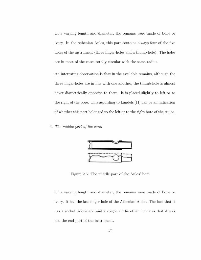
3. The middle part of the bore:

Figure 2.6: The middle part of the Aulos’ bore

Of a varying length and diameter, the remains were made of bone or

ivory. It has the last finger-hole of the Athenian Aulos. The fact that it

has a socket in one end and a spigot at the other indicates that it was

not the end part of the instrument.

17

One possible reason concerning why there had to be an extra part for the

fifth hole is that bones of suitable size for the Aulos were available only

in small lengths. Yet, Landels [11], has another approach according to

which, the distance from the fourth to the fifth hole is slightly reduced

if the hole that is covered by the little finger is slightly out of line with

the rest. This practice, used nowadays too in instruments like flutes, is

supposed to make the playing more convenient to the performer.

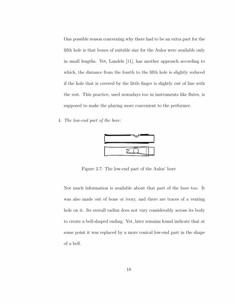
4. The low-end part of the bore:

Figure 2.7: The low-end part of the Aulos’ bore

Not much information is available about that part of the bore too. It

was also made out of bone or ivory, and there are traces of a venting

hole on it. Its overall radius does not vary considerably across its body

to create a bell-shaped ending. Yet, later remains found indicate that at

some point it was replaced by a more conical low-end part in the shape

of a bell.

18

2.3 Physical properties of single and

double-reed woodwind instruments

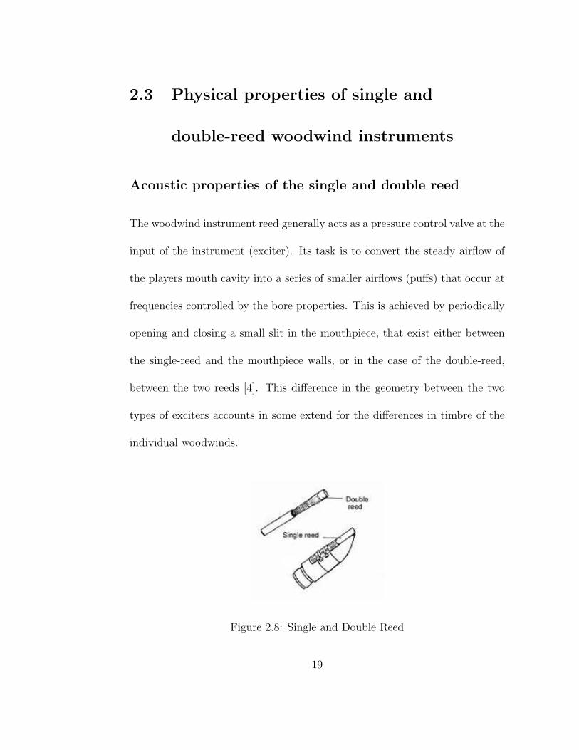
Acoustic properties of the single and double reed

The woodwind instrument reed generally acts as a pressure control valve at the

input of the instrument (exciter). Its task is to convert the steady airflow of

the players mouth cavity into a series of smaller airflows (puffs) that occur at

frequencies controlled by the bore properties. This is achieved by periodically

opening and closing a small slit in the mouthpiece, that exist either between

the single-reed and the mouthpiece walls, or in the case of the double-reed,

between the two reeds [4]. This difference in the geometry between the two

types of exciters accounts in some extend for the differences in timbre of the

individual woodwinds.

Figure 2.8: Single and Double Reed

19

It has been observed that reeds function properly in conditions where the

airflow inside the bore vibrates in such a way that creates maximum pressure

variation at the top end of the bore, next to the mouthpiece. Benade described

this condition in his work The Physics of Wood Winds [5] in the following way:

”In short, the operation of a cane reed calls for those vibrations in the air

column that produce maximum variation of pressure at the reed end of the

bore, and essentially zero fluctuations at the lower end...”

Moreover, Backus, who in 1961 first measured the vibrations of a single

reed, by recreating artificially the blowing conditions, discovered that for soft

notes, the slit of the reed almost never closed. On the other hand, the reed

operated in such a way that for greater applied pressures, and therefore louder

sounds, the gap opened and closed completely once every cycle [14].

Since the reed is controlled by pressure, that means that any changes in

it, apart from affecting the aperture in the way we described above, affect

the resulting tone quality/frequency too. For example, performers create the

well-known Vibrato effect by applying periodic changes in the lip-pressure.

Furthermore, changes in the frequency of the produced note, of the magnitude

of a semitone or less, can be achieved by using increased or decreased lip

pressure on the reed.

Finally, another characteristic of the woodwind reeds that is worth men-

20

tioning is the dependence of their response on the elevation of the location that

the performance is taking place. More specifically, since the reeds functional-

ity as an air valve depends on pressure, it is reasonable according to Scavone

[14] to expect changes in its response at considerably different elevations. The

reed is said to become more inflexible, by the performers. This defect can

be compensated by applying more oral cavity pressure than it was normally

needed.

Acoustic properties of the cylindrical bore

The resonator of woodwind instruments, that is the bore, plays a significant

role in the timbre of each one of them for several factors. First of all the pro-

duced frequency is controlled by its length and size. Moreover, the produced

overtones are totally controlled by its geometry. As we’ll explain later, conical

bores have all harmonics, whereas cylindrical ones have just the odd ones. Fi-

nally, the small mass and stiffness of the reed, give complete control over the

vibration and the produced pitch to the bore [5].

In order for a type of bore to be musically useful, it is necessary that the

ratios between the natural-mode frequencies remain constant, when the bore

is cut in smaller lengths from the low open end, as by opening the tone-holes.

In that way, the timbre of the instrument remains somehow the same for all

21

the instruments that belong to the same family. This theory is related to

the ability of using the same holes for producing notes in all the instrument

registers. Finally, it is also associated with the ability of over-blowing, on

which it is based the performance of wind instruments.

The only type of horns that fulfill these requirements are the Bessel ones,

for which the cross section of the bore is increased by some positive power of

the distance from the end of the bore. This exponent distinguishes between

the different shapes of horns. Benade [5] reports that, although there seems to

be and infinite number of bores that satisfy that condition, one for every pos-

itive power, in practice certain limitations posed by the nature of our hearing

system, reduce our choices to two, for which the exponent is equal to either

zero or two. In the first case belong the cylindrical bore instruments, such as

the clarinet and the flute, while in the later the conical bore ones, such as the

oboe, the bassoon and the saxophone.

In practice, although all woodwind instruments have shapes that corre-

spond to the two cases described above, none of them has a perfectly conical

or cylindrical figure. Yet, accurate representation of the wave propagation in

imperfectly shaped bores can be achieved by modeling these instruments in

terms of cylindrical and conical sections [14].

As we mentioned previously, the type of pipe in an instrument controls the

22

harmonics present in its produced sound and its fundamental wavelength. It

has been proved that in the case of open-open pipes the resonance frequencies

of the bore can be calculated by the following formula,

fo−o =nc

2Ln ∈ N

where n is the number of the harmonic, c is the speed of air and L is the length

of the bore, whereas in the case of open-closed ones by:

fo−c =(2n− 1)c

4Ln ∈ N

From the above equation we extract the information that open-open pipes have

a fundamental wavelength equal to two times the bores length and partials at

integer multiples of the fundamental frequency, while open-closed ones have a

fundamental wavelength equal to 4 times their bore length and partials at odd

integer multiples of the fundamental frequency.

In the case of finite length bores, that is for all musical instruments, trav-

eling waves face discontinuities at the ends of the bore. This impedance mis-

match causes part of the wave component to be transmitted into the discon-

tinuous medium and part of it to be reflected back into the pipe. Thus, the

wave variables of a finite length bore can be regarded as two superimposed

waves, an ingoing and outgoing one.

This observation is true for both types of bores. Yet, there is an important

difference in the case of the conical bores, since they are not symmetric about

23

their mid-point. Ingoing and outgoing wave propagation are different in this

case. The impedance of the waves traveling towards the end of the bore is the

complex conjugate of that of waves traveling away from the bore-end [14].

Finally, we have to mention that the waves inside a pipe are reflected due to

the described discontinuities in a frequency dependent manner. The frequency

dependent coefficient r is used to describe this fact and to indicate the ratio

of occurrence to reflected complex amplitudes in every frequency [14].

Acoustic properties of the tone-holes

The amount of side-holes present on the bore of different woodwind instru-

ments control the number of individual pitches, or scales produced by them.

The simplest approximation of the role of tone-holes in sound production is

to assume that a closed hole has no effect on the wave propagation, while an

open one causes the bore to behave as if it was truncated at that particular

place. In other words, finger-holes offer a set of alternative bore lengths to an

instrument [5].

In all the music cultures that are based on the western music system of

equal temperament, the tonehole placement and radii are related to the ra-

tio of a semitone 2112 . More specifically, the distance between two successive

toneholes will roughly be equal to x = 2112L, where L is the space between the

24

hole and the upper end of the air column [14]. Generally, the placement of the

holes has to be such in western instruments that the note sounding when all

the holes are open is the same with the first partial of the one sounding with

all the holes closed. Needless to say that in non-western music systems such

relationships between the distances of the holes are not necessarily the same.

Benade [5], was among the first who tried to define the relationship between

the size of the holes and their spacing. His theory was that the ratio of the air

present in a closed finger-hole to that present at the part of the bore between

two successive holes had to be the same throughout the instruments body.

That theory was confirmed by the structure of western, classical, woodwind

instruments, whose holes get bigger in radius as we move further down on the

instruments bores.

The holes dont just serve as cutting off mechanism of the bores in con-

venient distances from excitation, but they also play an important role on

the quality of the produced sounds. It has been discovered that closed holes

act, actually, as very sharp, low-pass filters that discriminate against the high

components of the vibration frequencies created by the reed. The propagation

wavenumber below that cut off frequency is real, whereas the one above it is

imaginary. Benade [5] made also the observation that only the first couple

of open holes can affect the behavior of the low frequency components of the

25

woodwinds.

According to Scavone [14], altering the size of the finger-holes can influence

the resulting tones in different ways:

1. Increasing the radius of a hole will cause all the resonant frequency com-

ponents below the cutoff frequency to rise.

2. Increasing the tonehole height will cause all the resonant frequency com-

ponents below the cutoff frequency to lower.

3. Reducing the keypad height of the first couple of holes on an instruments

bore will lower the frequency on its first harmonic.

These alterations, along with their affect of the resulting tone, are known to

and exercised by the woodwind manufacturers for a very long time. Yet, they

are not the only types of changes on the quality of the sound available. The

performer has also great control over the quality of the produced note. Attack

variations, for example, are controlled by the applied mouth pressure. Slight

changes on the pitch of the note are also feasible by leaving parts of the other-

wise closed holes halfway open. Finally, even the production of multiphonics

can be made possible, with the use of non-traditional fingering.

26

Chapter 3

Digital waveguide model of the

Aulos

3.1 Methodology

Extraction of Physical Measurements

Of all the archaeological remains of ancient Greek musical instruments avail-

able nowadays, those of the Auloi are the most informative. Yet the recon-

struction of a complete instrument out of those pieces remains a very difficult,

if not impossible, task, for reasons explained earlier. For the creation of an

acoustic model of the instrument in this paper, the necessary physical prop-

erties of its parts were extracted from fragments found in the Athenian Agora

27

excavation in Athens, Greece. [11] More specifically, fragments A (Inv. BI

593), C (Inv. BI 579), I (Inv. BI 630) and H (Inv. BI 594) were used as

models of the Aulos bulbs, the upper, middle and low-end part of the bore

respectively.

Two different models were created, one with a single and one with a double

reed, both of which consist of a mouthpiece with a reed and two bulbs, and the

three-part bore. The physical measurements of the fragments length, radius,

number, placement and size of the holes were extracted from Landels detailed

study and scaled graphs available at [11]1.

An estimation of the reeds length was based on Letters purely mathematical

approach of calculating the length on missing parts of an instrument based on

the relationship between the frequencies of two notes and the resulting interval.

[13] An interval can be expressed as the ratio of the higher frequency to the

lower one, which is equal to the length of the air column of the lower note to

that of the higher one. If one assumes that two holes in an instrument are a

certain interval apart, then the length of the reed can be easily extracted.

x+ Llowx+ Lhigh

= Interval (3.1)

Where x is the length of the reed and Llow and Lhigh the distance from the

top of the bulb to the lower and higher hole respectively and Interval is the

1A description of the data and the calculations done is available in Appendix A.

28

ratio of the resulting interval

For example if we assume that the interval between the first and the fourth

hole of the modeled Aulos is a perfect fourth, then:

x+ L1

x+ L4

=4

3⇔ x = 0.037m

Following that theory, five different reed lengths were calculated based on the

assumptions that the distances between different holes were a perfect fourth

or a perfect fifth. By combing that data to the already known distances

between the holes on the instruments bore, five different music scales were

calculated. The intervals between the produced frequencies of these scales

were converted into cents and compared to the known from the literature

ancient Greek scales2.

One can easily see that Letters approach is oversimplified and cannot be re-

garded as an accurate representation of the scales produced by an instrument,

since it completely ignores factors that can considerably affect the pitch of a

note, like the radius of the instruments bore, the size of the holes, the affect

of the reed itself on the resulting tone, and the control each player has over

the produced sound. Nevertheless, it gives an estimation of at least the length

of the reed and the resulting rough length of the instrument, which were used

for the waveguide digital model of the Aulos.

2All the calculations are available in Chapter 3

29

Digital waveguide modeling

The usual method of examining and modeling the acoustic behavior of wind

and string instruments is by dividing them into two basic parts that interact to

create the sound, the resonator and the exciter. In the case of the Aulos, these

will be the air column inside the bore and the reed respectively. In practice,

such separation is impossible since there are no clear boundaries between these

systems. Yet, this simple model has been used in many studies, [1], [3], [9],

[14], with considerably accurate results.

The Digital Waveguide (DW) technique simulates the wave propagation

along the instrument, in case of a woodwind one, along its bore, using delay-

lines. In this project the DW model and the related Matlab script were based

on the work done by Gary P. Scavone titled An Acoustic Analysis of Single-

Reed Woodwind Instruments with an Emphasis on Design and Performance

Issues and Digital Waveguide Modeling Techniques [14], and therefore the

structure of the model is the following: a non-linear excitation function models

the behavior of the reed, a bi-directional delay line models the resonator and

a digital reflection filter models the discontinuities created at the open end of

the pipe.

The script was modified to allow modeling of a 5 finger-hole plus a venting

hole instrument. The radii of the bore and holes were altered to match the

30

ones of the Aulos and in the case of the double-reed instrument different con-

stants and equations were added to describe the behavior of the new excitation

mechanism. Also, the two-port waveguide implementation, which utilizes four

second-order filter operators per hole, was picked to model the tone-holes.

Finally, the ability to choose between 5 different tunings of the instrument

and to record samples of a specified duration of the created sound was also

included in the scripts along with some error checking messages and default

values.

A more detailed description of the DW models of each of the instrument’s

parts follows.

31

3.2 Modeling the mouthpiece of a single and

of a double reed Aulos

The reed and the mouthpiece in woodwind instruments act as a pressured

control valve of the volume flow entering the reed, that controls and maintains

the oscillations of the air column in the bore at frequencies corresponding to

the resonant ones of the pipe. The opening area of the reed is controlled by the

difference in pressure P∆ between the inside of the reed area and the mouth

cavity and can be approximated with the following model

P∆ = Poc − Pr = k(S0 − S) (3.2)

where Poc and Pr are the pressure of the oral cavity and of the reed respectively,

k is the stiffness constant of the spring, and S0 is the opening area of the reed at

rest. For simplicity in these cases the oral cavity is regarded as large reservoir

of constant pressure and zero volume flow.

If we assume that the volume flow remains constant over the whole opening

area of the reed, we can apply the Bernoulli theorem between the mouth and

the reed to determine its flow qr.

qr = S

√2P∆

ρ(3.3)

where S is the opening area of the reed and rho the density of air.

32

These two mathematic formulas can apply to both single and double reed

instruments since studies have shown that the displacements of the reeds in

the latter case are symmetrical [9]. Yet, although the main principles are the

same, as the geometry alters between the two, more profound changes have to

be applied in order to transform the single reed into a double.

The single reed model

In the case of single reed instruments, like the clarinet, studies [14] [19] assume

continuity between the reed and the bore pressures Pr = Pb. The pressure of

the bore is regarded as the summation of the outgoing pressure traveling-wave

component p+ and the incoming pressure traveling-wave component from the

bore p−.

Pb = p+ + p− (3.4)

In this case, the driving force of the reed operation is controlled by:

P∆ = Poc(p+ + p−

)(3.5)

The reed to bore boundary is modeled by a reflection coefficient r, first sug-

gested by Smith in 1986 [19], whose response varies according to the difference

in pressure between the oral cavity and the bore P∆. The reeds volume flow

33

can be represented as the act of P∆ over the its acoustic impedance Zr,

qr =P∆

Zr(3.6)

whereas the bores one as,

qb = p+ − p−

Zb, (3.7)

where Zb is the impedance of the bore.

By assuming continuity between the reed and the bore flow qr = qb and

combing the resulting equation with (3.5), we get:

Poc − p+ + p−

Zr=p+ − p−

Zb(3.8)

which, when solved for the outgoing pressure wave p+ gives:

p+ = r

(p− − Poc

2

)+Poc2

(3.9)

where the pressure dependent coefficient r is equal to Zr−Zb

Zr+Zb[14].

Smith [19] also defined a term P+∆ such that

P+∆ =

Poc2− p− (3.10)

Which transformed equation (3.9) of the outgoing pressure wave into

p+ = −r(Poc2− p−

)+Poc2

(3.11)

p+ = −rP+∆ +

Poc2

(3.12)

34

In the case of woodwinds, Scavone suggested that there is a simple mathe-

matical expression that can describe the behavior of the pressure dependent

coefficient and results in a pretty realistic sound simulation of the instruments

[14].

r =

1 + m

(P+

∆ − pc)

if P+∆ − pc < 0

1 if P+∆ − pc ≥ 0

(3.13)

where pc is the necessary pressure to close the reed, which, when normalized,

equals to 1.

Values of P+∆ greater than pc indicate beating of the reed on the inner

surface of the mouthpiece and reflection of the ingoing pressure wave p−. When

the difference of pc from P+∆ is less than 1, partial reflection of p− and partial

transmission of Poc into the bore occur. Finally, for values of P+∆ less than 0,

the result is negative flow through the reed, since the bore pressure is greater

than the oral cavity one Pb > Poc [14].

The double-reed model

The basic difference between single and double-reed instruments, is that, in

the case of the latter, one cannot assume continuity between the pressure at

the beginning of the reed and at the beginning of the bore Pr 6= Pb. This is

mainly due to the difference in the geometry of the double reed, which causes

alterations in the volume flow. According to Almeida [1] these perturbations

35

are either created by jet reattachment, by formation of turbulent flow, or by

limitations posed by the duck.

A basic formula that can describe the relationship between the pressure at

the beginning of the reed Pr and that at the beginning of the bore Pb is given

below

Pr = Pb +1

2ρΨ

q2

S2r

(3.14)

where rho is the density of the air, Ψ is an empirical constant that controls

the dissipation factor, and Sr is the effective surface of the reed.

If we limit our approach to a quasi-static model, we can apply, once again,

the Bernoulli formula (2), to describe the volume flow across the reed. In this

case the opening of the reed S is controlled by

S = 2γz`α (3.15)

where α is the ratio of the flow to the duck section, 2z is the distance between

the two reeds, γ controls the geometry of the reed, and ` is the reeds slit length.

The driving force P∆ of the double reed operation can be calculated by

combining equations (1), (3), and (12) as follows:

P∆ = Poc −(p+ + p− +

1

2ρΨ

q2

S2r

)(3.16)

By taking into account formulas (6) and (13), and the Bernoulli Theorem (2),

we can eliminate the outgoing wave pressure p+ from the previous equation,

36

resulting in the following relationship between P∆, the mouth cavity pressure

Poc and the bore impedance Zb:

P∆ − Poc + Zb

(2γz`α

√2P∆

ρ

)+ 2p− +

1

2Ψ

(2γz`α)2 2P∆

S2r

= 0 (3.17)

If we set, for our convenience, x =√P∆(

1 +4Ψ (γz`α)2

S2r

)x2 +

(Zb (2γz`α)

√2

ρ

)x+

(2p− − Poc

)= 0 (3.18)

and calculate the roots of the resulting second order differential equation, we

will end up with two values, only one of which is of use to us, since pressure

is a force and must have a positive value.

x =−(Zb (γz`α)

√2ρ

)+

√(Zb (γz`α)

√2ρ

)2

−(

1 + 4Ψ(γz`α)2

S2r

)(2p− − Poc)

1 + 4Ψ(γz`α)2

S2r

(3.19)

The above gives us the relationship between the pressure of the oral cavity,

the ingoing pressure wave p− and the reeds driving force for double reed in-

struments, as opposed to (9), which gives that of the single reed.

In order, now, to estimate the value of p+ as a function of P∆ and the

reflection coefficient r, we need, once again, to assume continuity between the

reed - bore volume flow.

(2γz`α)√

2P∆

ρ= p+−p−

Zb⇔

p+ = p− + (2γz`α)Zb

√2P∆

ρ(3.20)

37

The linear acoustic behavior of the bore can also be described in terms of the

incoming and the outcoming pressure waves, which according to Almeida [1]

can be easily transformed using the reflection function.

p− = rp+ (3.21)

Having that in mind, the equation 18 can take its final form as follows:

p+ =2Zbγz`α

1− r

√2

ρP∆ (3.22)

38

3.3 Modeling the bore and the toneholes of

the Aulos

The models of the cylindrical bore and the toneholes in this paper were taken

from the PhD thesis of Gary P. Scavone, entitled An Acoustic Analysis of

Single-Reed Woodwind Instruments with an Emphasis on Design and Perfor-

mance Issues and Digital Waveguide Modeling Techniques, [14] and therefore,

very little remains to be said in this section.

The waveguide synthesis of the holes is based on a model described by

Keefe in 1990 that accurately presents a tonehole without taking into account

any adjacent-hole interactions [14]. Each finger-hole is represented by a two-

port junction function which models both series and shunt impedances. This

method requires four second-order filter operations for each hole.

Such mathematical descriptions of the tonehole behavior can only explain

two different hole-states, open or closed. Two approaches can be followed, in

order to take into account the different performances of the holes in states

between those two extremes. According to the first, the resulting filter coeffi-

cients can vary in time to compensate for the graduate opening and closing of

the holes. In the case of the second, it is possible to model that action with a

graduate cross-fade technique between the opening and closing filters.

39

Although such techniques are described in Scavones work [14] [15], none

of them is actually implemented into his waveguide model of the clarinet [14],

which was used in this project, leaving the program user with two choices,

that of an open and of a closed hole.

As far as the Aulos bore is concerned, a very simple model of a cylindrer

can be achieved by a Gaussian function, whose peak is centered at around

2cLb, where Lb is the length of the bore and c is the speed of air. The width

of the peak, which equals the time of the acoustic wave to travel from the reed

to the end of the bore and back, is according to Almeida [1], an indication of

the visco-thermal losses on the bore.

The cylindrical bore can be represented by a one-dimensional waveguide

model of its reflection coefficient, in cases of linear acoustic propagation. The

impedance mismatch that the traveling waves encounter at the end of the finite

length bore causes part of the wave to be transmitted to the new medium and

part of it to be reflected back. Therefore the bore of the Aulos is represented

as two superimposed pressure waves, an incoming p− and an outgoing one p+.

The output of the instrument y is the summation of those two pressure

waves p− and p−

y = p− + p+ (3.23)

40

In the case of the single reed Aulos, equation (3.23) takes the form of

ysingle = p− +Poc2− P∆ (3.24)

which, by taking into account the fact that p+ = p−

r, as explained before, and

making the necessary substitutions, can take the form of:

ysingle = p−(

1

r+ r

)(3.25)

When a double reed is used, on the other hand, things are a little bit different

and the final output of the instrument (3.23) takes the form of

ydouble = p− +(2γz`α)Zb

√2P∆

ρ

1− r(3.26)

where Zb is the characteristic impedance of the bore, α is the ratio of the flow

to the duck section, 2z is the distance between the two reeds, γ controls the

geometry of the reed, ` is the reeds slit length, P∆ is the reeds driving force,

and r is the reflectance coefficient.

Just a quick comparison of the two output-signals ysingle and ydouble

reveals the complexity of the double-reed mechanism over that of the single-

reed one. In the later case the output is just dependent on r and p−, whereas

in the first one, ydouble is a function of r, Zb, p− and P∆.

41

3.4 Interpretation and evaluation of the

resulting data

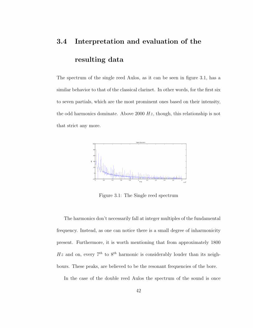
The spectrum of the single reed Aulos, as it can be seen in figure 3.1, has a

similar behavior to that of the classical clarinet. In other words, for the first six

to seven partials, which are the most prominent ones based on their intensity,

the odd harmonics dominate. Above 2000 Hz, though, this relationship is not

that strict any more.

0 0.2 0.4 0.6 0.8 1 1.2 1.4 1.6 1.8 2

x 104

−20

0

20

40

60

80

100Signal Spectrum

Freq

dB

Figure 3.1: The Single reed spectrum

The harmonics don’t necessarily fall at integer multiples of the fundamental

frequency. Instead, as one can notice there is a small degree of inharmonicity

present. Furthermore, it is worth mentioning that from approximately 1800

Hz and on, every 7th to 8th harmonic is considerably louder than its neigh-

bours. These peaks, are believed to be the resonant frequencies of the bore.

In the case of the double reed Aulos the spectrum of the sound is once

42

again dominated by the odd harmonics. This is perfectly understood, since

it’s the shape of the bore that is believed to control the harmonic content of a

sound and not the type of mouthpiece.

0 0.2 0.4 0.6 0.8 1 1.2 1.4 1.6 1.8 2

x 104

0

10

20

30

40

50

60

70

80

90Signal Spectrum

Freq

dB

Figure 3.2: The Double reed spectrum

Yet, as we can see in figure 3.2 this relationship is not that strict above

2000 Hz up until approximately 10 kHz. In this area we notice that the even

harmonics gain intensity, and although still softer than the odd ones, do play

a significant role in the high frequency content of the sound. Finally, one can

notice certain patterns, which reveal the bore’s resonance frequencies, and a

small degree of inharmonicity between the partials.

If we attempt, now, to compare the two spectrums (see figure 3.3), we

will see the affect of the two different reeds on the sound of cylindrical bore

woodwinds.

Two are the most apparent differences here. One concerns the energy

present in the harmonic content of the sounds. As we notice the partials don’t

43

0 1000 2000 3000 4000 5000 6000 7000 8000 9000 10000

−10

0

10

20

30

40

50

60

70

80

90

100Signal Spectrum

Freq

dB

Double ReedSingle Reed

Figure 3.3: Single and Double reed spectrum comparison

decay in equal ways and to the same degree. For reasons, which are beyond

the scope of this thesis, that have to do with the operation of the reeds, the

spectrum of the double reed carries considerably more energy.

The other one has to do with the intonation of the two sounds, which

appear in the spectum to be slightly detuned, even though they were created

on the same bore and with exactly the same fingering. We will revisit this

aspect in chapter 4, where we deal with the Aulos’ scales.

44

Chapter 4

The Aulos’ scales

For the purposes of this research paper, two different models of the Ancient

Greek Aulos were built using MATLAB, a single and a double-reed one, based

on the fragments found in the Athenian Agora excavation in Athens, Greece.

Both of the instruments consist of a mouthpiece, of two bulbs, and a three

part bore. Yet, as we said before, there is no information available on the reed

of the instrument.

It is understood that an estimation of the sound of the instrument and its

produced scales cannot be considered exact without the presence of the reed

physical properties. Letters, therefore, came up with a purely mathematical

method of estimating the reeds length and the possible scales played by an

Aulos based on the relationship between the frequencies of two notes and the

45

resulting interval [13].

Although this approach of estimating scales cannot be treated as accurate,

since it disregards all the other factors that play a significant role in the pro-

duction of sound, such as the radius of the instrument’s bore, and holes, the

affect of the reed itself on the resulting tone, and the control each player has

over the produced sound, it was used here, as we claimed before, in order to

calculate just the length x of the reed.

Moreover, the presence of 5 toneholes on the bore of the instruments re-

mains a mystery, since the ancient Greek music was based on the use of tetra-

chords. One may use this fact as evidence that more than one tetrachords

were played with the same instrument. Yet, since resulting intervals between

adjacent holes are not equal, like in the case of equal temperament, this will

require some changes on the instrument’s effective length.

At first, such a fact may seem impractical, because adding to or removing

parts, like bulbs for example, from the instrument while performing is unfeasi-

ble. K. Schlesinger, however, suggested the theory of the moving mouthpiece

[18]. According to that, the player could move from one tetrachord to the

other easily by pushing of pulling the reed in and out of the mouthpiece, af-

fecting in that way its effective length. In such a system, the two higher holes

of the lower tetrachord may be used as the two lower holes of the higher one.

46

What follows is a description of the calculations of the scales for the re-

sulting single and double reed Aulos.

47

4.1 Calculation of the resulting scales

For the purpose of estimating the length of the reed in the Aulos, five different

assumptions were made:

1. The interval between all holes open and the top three holes closed is a

perfect fouth: 1.

x+ L0

x+ L3

=4

3⇔ x = 0.042 m

2. The interval between the first and the fourth hole is a perfect fouth:

x+ L1

x+ L4

=4

3⇔ x = 0.037 m

3. The interval between the second and the fifth hole is a perfect fouth:

x+ L2

x+ L5

=4

3⇔ x = 0.0729 m

4. The interval between all holes open and the top four holes closed is a

perfect fifth:

x+ L0

x+ L4

=3

2⇔ x = 0.029 m

5. The interval between the first and the fifth hole is a perfect fifth:

x+ L1

x+ L5

=3

2⇔ x = 0.0476 m

1A description of the lengths of each fragment used, and the distances between the holesis available in Appendix.

48

As one can easily see, all the reed lengths, with maybe the exception of

that in the third case, fall within a reasonable range. There are two possible

reasons why the length of the reed is bigger in assumption number 3. Either

the selected ratio of the second to the fifth hole is not correct, or the dimensions

of the selected fragment, which corresponds to the part of the bore that has

the fifth hole, don’t match those of the rest of the instrument parts. Both

cases are expected to occur anywhere in the model, since it is well understood

that a model which is based on parts that is not sure if they belong together

can only be regarded as an approximation of a real instrument and not as its

accurate representation.

In any case, the adjustments of the reed length that need to be made

in order for the player to move from one tetrachord to the other are of the

magnitude of a centimeter, and therefore easy to achieve. This may lead us to

think that Schlesinger’s theory of the moving mouthpiece can be considered

possible.

The following table contains the distances from the excitation mechanism,

to each hole and to the end of the bore, for every one of the assumptions

described before. If we look at the resulting data, we can see that the re-

sulting lengths for each scale are more or less the same, with the exceptions

explained before. More specifically, for example, the length of the mouthpiece

49

is approximately 21 cm, and that of the bore is around 50 cm.

Assum. 1 Assum. 2 Assum. 3 Assum. 4 Assum. 5Lmpiece (m) 0.221 0.216 0.2519 0.208 0.2266L1 (m) 0.245 0.24 0.2759 0.232 0.2506L2 (m) 0.27 0.265 0.3009 0.257 0.2756L3 (m) 0.298 0.293 0.3289 0.285 0.3036L4 (m) 0.325 0.32 0.3559 0.312 0.3306L5 (m) 0.3503 0.3453 0.3812 0.3373 0.3559Lvent (m) 0.4582 0.4532 0.4891 0.4452 0.4638Lbore (m) 0.5045 0.4995 0.5354 0.4915 0.5101

As far as the calculation of the resulting scales of each of the 5 assumptions

is concerned, we avoided following Letters’ approach of converting the above

lengths of the air columns into cents [13], because as it was proven in a test, it is

really inaccurate and creates considerable deviations from the actual sounding

scales of the models. Instead the following formula was used to convert from

frequency ratios to cents.

cents =1200

log 2log

(fhigh

flow

)(4.1)

The frequencies of the first harmonic of the notes that resulted from each

of the previous assumptions were calculated in MATLAB. By doing so, the

estimation of the produced notes is not simply a function of lengths, but takes,

also, into account factors such as the type of the reed, the length and radius of

the bore, and the radius and placement of the holes on the bore, that make it

more accurate. Furthermore, two sets of frequencies and interval ratios were

50

calculated since it was noticed that the resulting notes of the single and the

double reed model had slightly different frequencies.

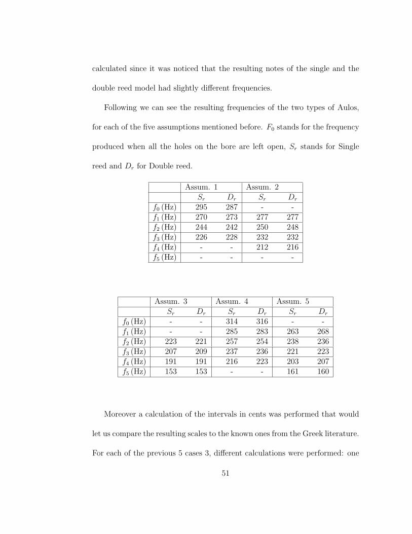
Following we can see the resulting frequencies of the two types of Aulos,

for each of the five assumptions mentioned before. F0 stands for the frequency

produced when all the holes on the bore are left open, Sr stands for Single

reed and Dr for Double reed.

Assum. 1 Assum. 2Sr Dr Sr Dr

f0 (Hz) 295 287 - -f1 (Hz) 270 273 277 277f2 (Hz) 244 242 250 248f3 (Hz) 226 228 232 232f4 (Hz) - - 212 216f5 (Hz) - - - -

Assum. 3 Assum. 4 Assum. 5Sr Dr Sr Dr Sr Dr

f0 (Hz) - - 314 316 - -f1 (Hz) - - 285 283 263 268f2 (Hz) 223 221 257 254 238 236f3 (Hz) 207 209 237 236 221 223f4 (Hz) 191 191 216 223 203 207f5 (Hz) 153 153 - - 161 160

Moreover a calculation of the intervals in cents was performed that would

let us compare the resulting scales to the known ones from the Greek literature.

For each of the previous 5 cases 3, different calculations were performed: one

51

for the single reed model, one for the double reed model, and another one using

Letters’ mathematical approach of converting air column lengths into scales.

Assum. 1 Assum. 2Sr Dr L Sr Dr L

f0

f1153.3 86.6 178.5 - - -

f1

f2175.3 208.7 168.2 177.5 191.5 171.5

f2

f3132.7 103.2 170.8 129.4 115.5 173.9

f3

f4- - - 156 123.7 153.6

f4

f5- - - - - -

Assum. 3 Assum. 4Sr Dr L Sr Dr L

f0

f1- - - 167.8 190.9 189

f1

f2- - - 179 187.1 177.1

f2

f3128.9 96.7 154 140.2 127.2 179

f3

f4139.3 155.9 136.6 160.6 98 156.7

f4

f5384 384 118.9 - - -

Assum. 5Sr Dr L

f0

f1- - -

f1

f2173 222.1 164.6

f2

f3128.3 98 167.5

f3

f4147 128.9 147.4

f4

f5401.3 445.9 127.7

The computed calculations above can be treated as proof of the fact that

the instrument’s physical properties affect considerably the resulting tones.

This is not only understood by the deviation of the calculations made with

52

Letters’ model from the other two, which is the most apparent, but also from

the differences between the single and the double reed instrument frequencies

and intervals. This observed variation can also be treated as evidence of the

fact that the bore of the woodwinds, although the most important, is definitely

not the only factor that affects the resulting tones.

53

4.2 Evaluation of the resulting scales and

comparison with the known ancient

Greek ones

Unfortunately, no match with any of the known ancient Greek scales was made

possible in any of the above cases. This can be the result of various reasons,

all of which are understandable and were more or less expected to occur at

some point in the project.

First of all, the fragments used to compose this Physical Model of the

Aulos don’t necessarily belong to the same instrument, or to the same bore.

Most likely, they belonged to different instruments, built by various people at

different years during the 5th and the 4th century B.C.

Moreover, this model utilizes only one bore, although we know that the

Aulos was a two double bore instrument. The reason of that omission is that

no information is available on that second bore, mainly because there are not

enough fragments found to completely reconstruct an Aulos, and therefore

extract with relative certainty each bores physical properties. Yet, it is under-

stood that the presence of a second bore in this model will considerably affect

the resulting tones and their intervals.

Furthermore, the waveguide approach was inevitably based on the way

54

acoustic properties of woodwind instruments exist now. In other words, it was

based on instruments whose level of perfection, as far as their construction is

concerned, is far from that of the Aulos. For example, Schlesinger [18], who

was among the first to attempt the physical reconstruction of an Aulos, wrote

in her report:

”The type of double reed mouthpiece in use on the primitive Greek Aulos was

obviously not the highly sophisticated oboe reed of the present day, but the

simple ripe of wheat or oat stalk, plucked from the cornfield”.

Such a difference in the building standards is also expected to affect the pro-

duced sounds to a great extend.

Finally, this model doesn’t take into account the control that the performer

has over the sound of his/her instrument. This was merely done for two

reasons. First of all, the complexity that such an approach would have added

to the waveguide model goes well beyond the scope of this project. Second,

there is no information available, at least to the knowledge of the author, that

contains information about the performing techniques of wind instruments in

Ancient Greece.

However, although all the above factors discriminate against the possible

accuracy of the resulting Aulos’ sound and scales, it is believed that by trial

and error, the correct combinations of fragments and reed lengths, that lead

55

to more accurate scales, can be made. In any case, though, these results can

probably also be taken into account when the validity of the Ancient Greek

music theory, the way it is interpreted nowadays, is under question.

56

Chapter 5

Conclusions/ Future work

This study attempted to reconstruct the Ancient Greek Aulos based on waveg-

uide synthesis. The two resulting models, which were based on the fragments

found in the Athenian Agora excavation, and their related studies, managed

to represent the Aulos to a certain extent and in way that wasn’t attempted

before, at least to the knowledge of the author.

Work still remains to be done, though, in the fields of the sound realism

and recreation of the ancient Greek scales. The imperfection of the instru-

ments manufacture, as described above, has to be taken into account in the

MATLAB algorithm along with some options of performance control. Fur-

thermore, the combination of bore’s and reed’s length, along with the appro-

priate fingering for the creation of the Aulos’ scales, has to be revisited.

57

Chapter 6

Appendix

6.1 Physical Measurements of the Athenian

Aulos fragments

The following table contains data that was extracted from Landels’ description

of the Aulos’ fragments found in the Athenian Agora excavation [11]. For the

purposes of this paper fragments A, C, I and H were used.

Mouthpiece Upper Bore Middle Bore Low end BoreLength (cm) 8.95 11.3 9.15 7.9

Bore radius (cm) 1.85/2 1.6/2 1.8/2 1.8/2Hole radius (cm) - 0.85/2 0.95/2 -

Distance form the center of each hole to the upper part of the correspond-

ing fragment:

59

Fragment C:

H1 = 0.024m, H2 = 0.049m, H3 = 0.077m , IH4 = 0.104 m

Fragment I:

H5 = 0.0163 m

Fragment H:

Hvent = 0.0327 m

60

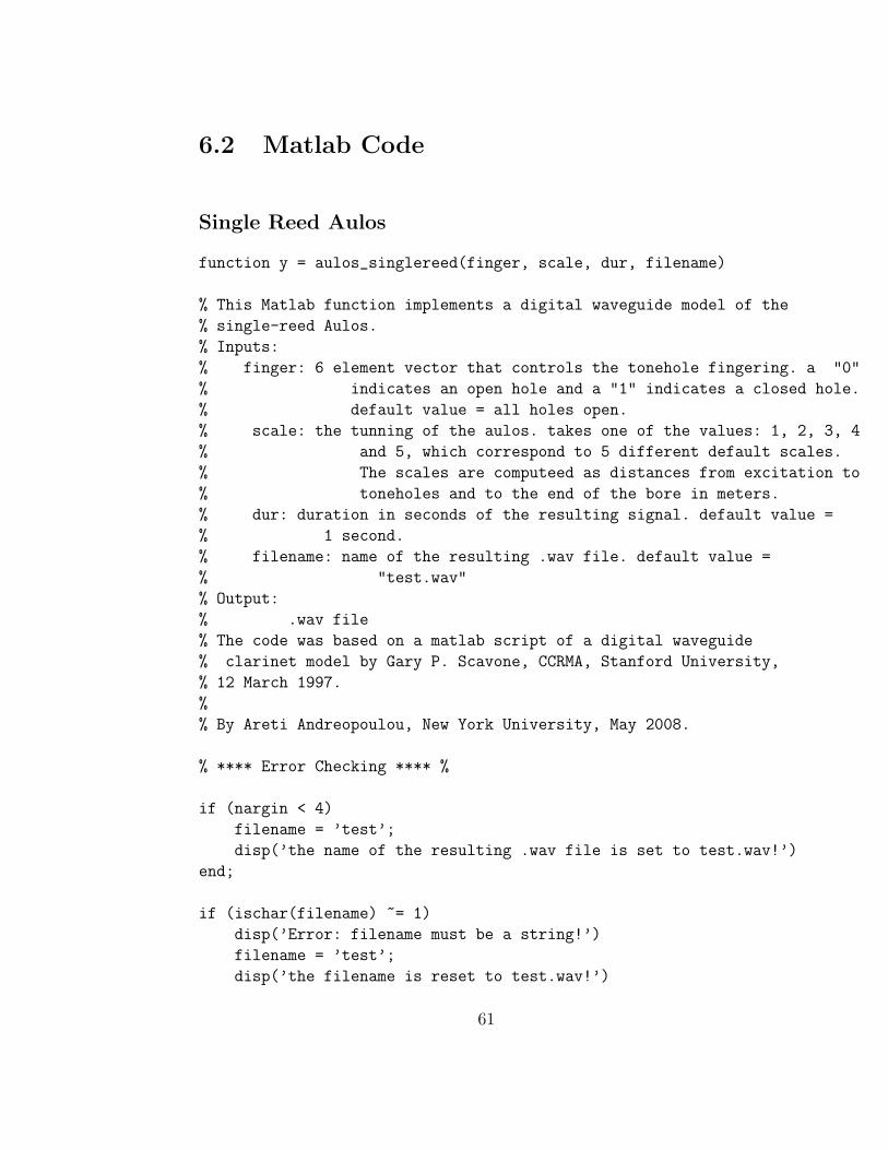
6.2 Matlab Code

Single Reed Aulos

function y = aulos_singlereed(finger, scale, dur, filename)

% This Matlab function implements a digital waveguide model of the

% single-reed Aulos.

% Inputs:

% finger: 6 element vector that controls the tonehole fingering. a "0"

% indicates an open hole and a "1" indicates a closed hole.

% default value = all holes open.

% scale: the tunning of the aulos. takes one of the values: 1, 2, 3, 4

% and 5, which correspond to 5 different default scales.

% The scales are computeed as distances from excitation to

% toneholes and to the end of the bore in meters.

% dur: duration in seconds of the resulting signal. default value =

% 1 second.

% filename: name of the resulting .wav file. default value =

% "test.wav"

% Output:

% .wav file

% The code was based on a matlab script of a digital waveguide

% clarinet model by Gary P. Scavone, CCRMA, Stanford University,

% 12 March 1997.

%

% By Areti Andreopoulou, New York University, May 2008.

% **** Error Checking **** %

if (nargin < 4)

filename = ’test’;

disp(’the name of the resulting .wav file is set to test.wav!’)

end;

if (ischar(filename) ~= 1)

disp(’Error: filename must be a string!’)


disp(’the filename is reset to test.wav!’)

61

end;

if (nargin < 3)

dur = 0.5;

disp(’the duration of the tone is set to 0.5 sec!’)

end;

if (ischar(dur) == 1)

disp(’Error: duration must be a number!’)

return;

end;

if (nargin < 2)

scale = 1;

disp(’the first sample scale is selected!’)

end;

if (scale<=0 || scale > 5)

disp(’Error: scale must have one of the following values: 1, 2, 3, 4

or 5!’)

return;

end;

if ( scale / floor(scale) ~= 1)


or 5!’)

return;

end;

if (ischar(scale) == 1)


or 5!’)

return;

end;

if (nargin < 1)

finger = [0, 0, 0, 0, 0, 0];

disp(’finger is set to [0, 0, 0, 0, 0, 0]!’)

end;

62

if (ischar(finger) == 1)

disp(’Error: finger must be a 6 element vector’)

return;

end;

if (length(finger) ~= 6)


return;

end;

if (sum(finger)<0 || sum(finger)>6)

disp(’Error: the vector can be filled only with ones and zeros’)

return;

end;

% *** Signal Parameters *** %

fs = 44100; % sampling rate

N = dur*fs; % number of samples to compute

% ******* Air Column Parameters ******* %

c = 347.23; % speed of sound in air (meters/second)

ra = 0.0175/2; % radius of bore (meters) %% ARETI

tw = 0.0034; % shortest tonehole height (meters)

rc = 0.0005; % tonehole radius of curvature (meters)

% **** Distances From Excitation To Toneholes & End (m) **** %

if (scale == 1)

L = [0.245, 0.27, 0.298, 0.325, 0.3503, 0.4582, 0.5045];

end;

if (scale == 2)

L = [0.24, 0.265, 0.293, 0.32, 0.3453, 0.4532, 0.4995];

end;

if (scale == 3)

L = [0.2759, 0.3009, 0.3289, 0.3559, 0.3812, 0.4891, 0.5354];

end;

63

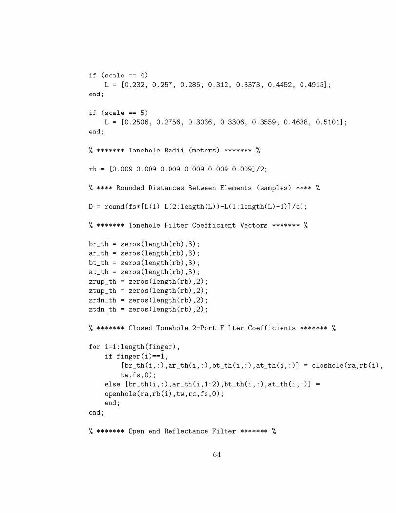
if (scale == 4)

L = [0.232, 0.257, 0.285, 0.312, 0.3373, 0.4452, 0.4915];

end;

if (scale == 5)

L = [0.2506, 0.2756, 0.3036, 0.3306, 0.3559, 0.4638, 0.5101];

end;

% ******* Tonehole Radii (meters) ******* %

rb = [0.009 0.009 0.009 0.009 0.009 0.009]/2;

% **** Rounded Distances Between Elements (samples) **** %

D = round(fs*[L(1) L(2:length(L))-L(1:length(L)-1)]/c);

% ******* Tonehole Filter Coefficient Vectors ******* %

br_th = zeros(length(rb),3);

ar_th = zeros(length(rb),3);

bt_th = zeros(length(rb),3);

at_th = zeros(length(rb),3);

zrup_th = zeros(length(rb),2);

ztup_th = zeros(length(rb),2);

zrdn_th = zeros(length(rb),2);

ztdn_th = zeros(length(rb),2);

% ******* Closed Tonehole 2-Port Filter Coefficients ******* %

for i=1:length(finger),

if finger(i)==1,

[br_th(i,:),ar_th(i,:),bt_th(i,:),at_th(i,:)] = closhole(ra,rb(i),

tw,fs,0);

else [br_th(i,:),ar_th(i,1:2),bt_th(i,:),at_th(i,:)] =

openhole(ra,rb(i),tw,rc,fs,0);

end;

end;

% ******* Open-end Reflectance Filter ******* %

64

[b_open,a_open] = openpipe(1,2,ra,fs,0);

z_open = [0 0];

% ******* Boundary-Layer Losses ******* %

% The air column lengths between toneholes are short, so that losses

% will be small in these sections. Further, such losses can be

% commuted with fractional-delay filters (which are not incorporated

% here). In this model, boundary-layer losses are only included for

% the first, long cylindrical bore section.

[b_boundary,a_boundary] = boundary(2,2,ra,fs,D(1),0);

z_boundary = zeros(2,2);

% ******* Initialize delay lines ******* %

y = zeros(1,N); % initialize output vector

dl1 = zeros(2,D(1));







ptr = ones(length(rb)+1);

upin2pt = zeros(size(rb));

dnin2pt = zeros(size(rb));

p_oc = 0; % initial oral cavity pressure

pinc = 0.01; % oral cavity pressure increment

% *************************************** %

% %

% Delay Line %

% |-------------------------------| %

% ^ %

% pointer %

% %

% >>--- pointer increments --->> %

% %

65

% *************************************** %

% The pointer initially points to each delay line output.

% We can take the output and calculate a new input value

% which is placed where the output was taken from. The

% pointer is then incremented and the process repeated.

% ******* Run Loop Start ******* %

for i = 1:N,

pbminus = dl1(2,ptr(1));

upin2pt = [dl1(1,ptr(1)), dl2(1,ptr(2)), dl3(1, ptr(3)), dl4(1, ptr(4)),

dl5(1, ptr(5)), dl6(1, ptr(6))];

dnin2pt = [dl2(2,ptr(2)), dl3(2,ptr(3)), dl4(2, ptr(4)), dl5(2, ptr(5)),

dl6(2, ptr(6)), dl7(2, ptr(7))];

% ******* Boundary-Layer Loss Filter Calculations ******* %

[upin2pt(1),z_boundary(1,:)] = filter(b_boundary,a_boundary,

upin2pt(1),z_boundary(1,:));

[pbminus,z_boundary(2,:)] = filter(b_boundary,a_boundary,

pbminus,z_boundary(2,:));

% ******* Open-end Filter Calculations ******* %

[dl7(2,ptr(7)),z_open] = filter(b_open,a_open,dl7(1,ptr(7)),z_open);

% ***** First Tonehole Calculations ***** %

[temp1,zrup_th(1,:)] = filter(br_th(1,:),ar_th(1,:),upin2pt(1),

zrup_th(1,:));

[temp2,ztdn_th(1,:)] = filter(bt_th(1,:),at_th(1,:),dnin2pt(1),

ztdn_th(1,:));

dl1(2,ptr(1)) = temp1 + temp2;

[temp1,zrdn_th(1,:)] = filter(br_th(1,:),ar_th(1,:),dnin2pt(1),

zrdn_th(1,:));

[temp2,ztup_th(1,:)] = filter(bt_th(1,:),at_th(1,:),upin2pt(1),

ztup_th(1,:));


66

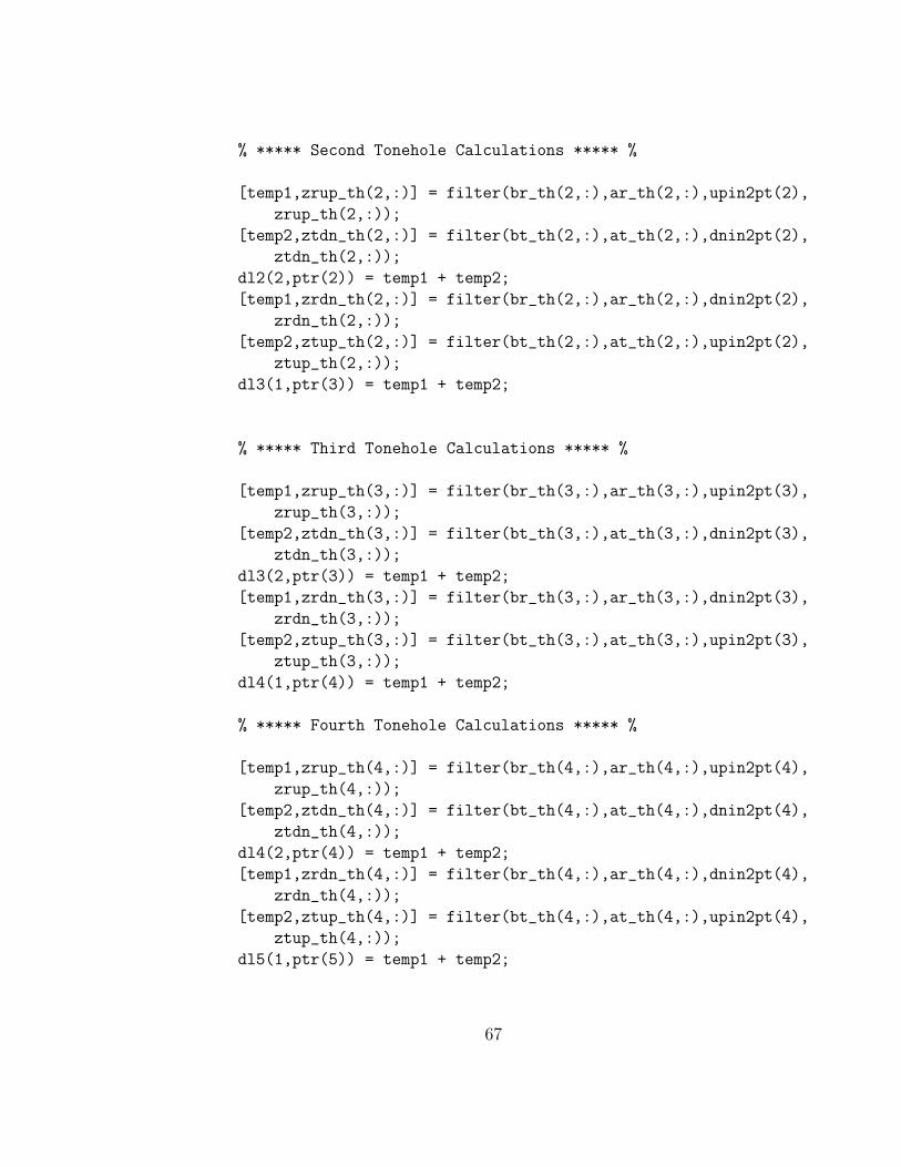
% ***** Second Tonehole Calculations ***** %


zrup_th(2,:));


ztdn_th(2,:));



zrdn_th(2,:));


ztup_th(2,:));


% ***** Third Tonehole Calculations ***** %


zrup_th(3,:));


ztdn_th(3,:));



zrdn_th(3,:));


ztup_th(3,:));


% ***** Fourth Tonehole Calculations ***** %


zrup_th(4,:));


ztdn_th(4,:));



zrdn_th(4,:));


ztup_th(4,:));


67

% ***** Fifth Tonehole Calculations ***** %


zrup_th(5,:));


ztdn_th(5,:));



zrdn_th(5,:));


ztup_th(5,:));


% ***** Sixth Tonehole Calculations ***** %


zrup_th(6,:));


ztdn_th(6,:));



zrdn_th(6,:));


ztup_th(6,:));


% ******* Excitation Calculations ******* %

p_delta = 0.5*p_oc - pbminus;

% ****** Pressure-Dependent Reflection Coefficient ****** %

refl = 0.7 + 0.4*p_delta;

if refl > 1.0

refl = 1.0;

end;

dl1(1,ptr(1)) = 0.5*p_oc - p_delta*refl;

% The system output is determined at the input to the air

68

% column. The oral cavity is incremented until it reaches

% the desired value.

y(i) = pbminus + dl1(1,ptr(1));

if p_oc < 1,

p_oc = p_oc + pinc;

end;

% ****** Increment Pointers & Check Limits ****** %

for j=1:length(L),

ptr(j) = ptr(j) + 1;

if ptr(j) > D(j),

ptr(j) = 1;

end;

end;

end;

% *** Plot, Play and Wavwrite *** %

norm_y = y./max(abs(y));

figure(1)

plot(norm_y, ’m’)

title(’Signal Output’);

xlabel(’Samples’);

ylabel(’Signal Level’);

sound(norm_y,fs);

wavwrite(norm_y, fs, 16, filename);

SIG = abs(fft(y/max(abs(y)),40000 ));

X = 20*log10(SIG);

figure(2)

plot(X(1:(length(X)/2)+1));

title(’Signal Spectrum’);

xlabel(’Freq’);

ylabel(’dB’);

69

Double Reed Aulos

function y = aulos_doublereed(finger, scale, dur, filename)

% This Matlab function implements a digital waveguide model of the

% double-reed Aulos.

% Inputs:

% finger: 6 element vector that controls the tonehole fingering. a "0"

% indicates an open hole and a "1" indicates a closed hole.

% default value = all holes open.

% scale: the tunning of the aulos. takes one of the values: 1, 2, 3, 4

% and 5, which correspond to 5 different default scales.

% The scales are computeed as distances from excitation to

% toneholes and to the end of the bore in meters.

% dur: duration in seconds of the resulting signal. default value =

% 1 second.

% filename: name of the resulting .wav file. default value =

% "test.wav"

% Output:

% .wav file

% The code was based on a matlab script of a digital waveguide

% clarinet model by Gary P. Scavone, CCRMA, Stanford University,

% 12 March 1997.

%

% By Areti Andreopoulou, New York University, May 2008.

% **** Error Checking **** %

if (nargin < 4)


disp(’the name of the resulting .wav file is set to test.wav!’)

end;

if (ischar(filename) ~= 1)

disp(’Error: filename must be a string!’)


disp(’the filename is reset to test.wav!’)

70

end;

if (nargin < 3)

dur = 0.5;

disp(’the duration of the tone is set to 0.5 sec!’)

end;

if (ischar(dur) == 1)

disp(’Error: duration must be a number!’)

return;

end;

if (nargin < 2)

scale = 1;

disp(’the first sample scale is selected!’)

end;

if (scale<=0 || scale > 5)


or 5!’)

return;

end;

if ( scale / floor(scale) ~= 1)


or 5!’)

return;

end;

if (ischar(scale) == 1)


or 5!’)

return;

end;

if (nargin < 1)

finger = [0, 0, 0, 0, 0, 0];

disp(’finger is set to [0, 0, 0, 0, 0, 0]!’)

end;

71

if (ischar(finger) == 1)


return;

end;

if (length(finger) ~= 6)


return;

end;

if (sum(finger)<0 || sum(finger)>6)

disp(’Error: the vector can be filled only with ones and zeros’)

return;

end;

% *** Signal Parameters *** %

fs = 44100; % sampling rate

N = dur*fs; % number of samples to compute

% ******* Air Column Parameters ******* %

c = 347.23; % speed of sound in air (meters/second)

ra = 0.0175/2; % radius of bore (meters)

tw = 0.0034; % shortest tonehole height (meters)

rc = 0.0005; % tonehole radius of curvature (meters)

% ****** Physical constants ****** %

rho = 1.1769; % air density

alfa =0.6; % ratio of the flow to the duct section

l = 4.6*10^-3; % slit length of the reed

z = 0.5*10^-3; % distance between the reeds

gama = 1/2; % geometry of the reed

Sr =2*(5*10^-3)*0.042; % area of the reed

psi = 100; % dissipation factor

Sb = pi*ra^2; % area of the bore

Zob = rho*c/Sb; % the characteristic impedance of the bore

72

% ******* Distances From Excitation To Toneholes & End (m) ******* %

if (scale == 1)

L = [0.245, 0.27, 0.298, 0.325, 0.3503, 0.4582, 0.5045];

end;

if (scale == 2)

L = [0.24, 0.265, 0.293, 0.32, 0.3453, 0.4532, 0.4995];

end;

if (scale == 3)

L = [0.2759, 0.3009, 0.3289, 0.3559, 0.3812, 0.4891, 0.5354];

end;

if (scale == 4)

L = [0.232, 0.257, 0.285, 0.312, 0.3373, 0.4452, 0.4915];

end;

if (scale == 5)

L = [0.2506, 0.2756, 0.3036, 0.3306, 0.3559, 0.4638, 0.5101];

end;

% ******* Tonehole Radii (meters) ******* %

rb = [0.009 0.009 0.009 0.009 0.009 0.009]/2;

% ******* Rounded Distances Between Elements (samples) ******* %

D = round(fs*[L(1) L(2:length(L))-L(1:length(L)-1)]/c);

% *** Initialize Empty Vectors *** %

PB = [];

DL = [];

% ******* Tonehole Filter Coefficient Vectors ******* %

br_th = zeros(length(rb),3);

ar_th = zeros(length(rb),3);

bt_th = zeros(length(rb),3);

73

at_th = zeros(length(rb),3);

zrup_th = zeros(length(rb),2);

ztup_th = zeros(length(rb),2);

zrdn_th = zeros(length(rb),2);

ztdn_th = zeros(length(rb),2);

% ******* Closed Tonehole 2-Port Filter Coefficients ******* %

for i=1:length(finger),

if finger(i)==1,

[br_th(i,:),ar_th(i,:),bt_th(i,:),at_th(i,:)] =

closhole(ra,rb(i),tw,fs,0);

else [br_th(i,:),ar_th(i,1:2),bt_th(i,:),at_th(i,:)] =

openhole(ra,rb(i),tw,rc,fs,0);

end;

end;

% ******* Open-end Reflectance Filter ******* %

[b_open,a_open] = openpipe(1,2,ra,fs,0);

z_open = [0 0];

% ******* Boundary-Layer Losses ******* %

% The air column lengths between toneholes are short, so that losses

% will be small in these sections. Further, such losses can be

% commuted with fractional-delay filters (which are not incorporated

% here). In this model, boundary-layer losses are only included for

% the first, long cylindrical bore section.

[b_boundary,a_boundary] = boundary(2,2,ra,fs,D(1),0);

z_boundary = zeros(2,2);

% ******* Initialize delay lines ******* %

y = zeros(1,N); % initialize output vector





74




ptr = ones(length(rb)+1);

upin2pt = zeros(size(rb));

dnin2pt = zeros(size(rb));

p_oc = 0; % initial oral cavity pressure

pinc = 0.01; % oral cavity pressure increment

% *************************************** %

% %

% Delay Line %

% |-------------------------------| %

% ^ %

% pointer %

% %

% >>--- pointer increments --->> %

% %

% *************************************** %

% The pointer initially points to each delay line output.

% We can take the output and calculate a new input value

% which is placed where the output was taken from. The

% pointer is then incremented and the process repeated.

% ******* Run Loop Start ******* %

for i = 1:N,

pbminus = dl1(2,ptr(1));

upin2pt = [dl1(1,ptr(1)), dl2(1,ptr(2)), dl3(1, ptr(3)), dl4(1, ptr(4)),

dl5(1, ptr(5)), dl6(1, ptr(6))];

dnin2pt = [dl2(2,ptr(2)), dl3(2,ptr(3)), dl4(2, ptr(4)), dl5(2, ptr(5)),

dl6(2, ptr(6)), dl7(2, ptr(7))];

% ******* Boundary-Layer Loss Filter Calculations ******* %

75

[upin2pt(1),z_boundary(1,:)] = filter(b_boundary,a_boundary,

upin2pt(1),z_boundary(1,:));

[pbminus,z_boundary(2,:)] = filter(b_boundary,a_boundary,

pbminus,z_boundary(2,:));

% ******* Open-end Filter Calculations ******* %

[dl7(2,ptr(7)),z_open] = filter(b_open,a_open,dl7(1,ptr(7)),z_open);

% ***** First Tonehole Calculations ***** %


zrup_th(1,:));


ztdn_th(1,:));



zrdn_th(1,:));


ztup_th(1,:));


% ***** Second Tonehole Calculations ***** %


zrup_th(2,:));


ztdn_th(2,:));



zrdn_th(2,:));


ztup_th(2,:));


% ***** Third Tonehole Calculations ***** %


zrup_th(3,:));

76


ztdn_th(3,:));



zrdn_th(3,:));


ztup_th(3,:));


% ***** Fourth Tonehole Calculations ***** %


zrup_th(4,:));


ztdn_th(4,:));



zrdn_th(4,:));


ztup_th(4,:));


% ***** Fifth Tonehole Calculations ***** %


zrup_th(5,:));


ztdn_th(5,:));



zrdn_th(5,:));


ztup_th(5,:));


% ***** Sixth Tonehole Calculations ***** %


zrup_th(6,:));


77

ztdn_th(6,:));



zrdn_th(6,:));


ztup_th(6,:));


% ******* Excitation Calculations ******* %

x = -(Zob*2*gama*z*l*alfa*sqrt((2/rho)) + sqrt(8*

(((Zob*gama*z*l*alfa)^2)/rho)-4*(1+ (4*psi*(gama*z*l.*alfa)

.^2)/Sr^2)*(2*pbminus - p_oc)))/(2*(1+(4*psi*(gama*z*l.*alfa).^2)

/Sr^2));

% ****** Pressure-Dependent Reflection Coefficient ****** %

refl = -0.7 + 0.4.*x;

if refl > 1

refl = 1;

end;

dl1(1,ptr(1)) = 2*Zob*gama*z*l*alfa*x*sqrt(2/rho)./(1-refl+eps);

PB = [PB,pbminus];

DL = [DL,dl1(1,ptr(1))];

% The oral cavity is incremented until it reaches the desired value.

if p_oc < 1

p_oc = p_oc + pinc;

end;

% ****** Increment Pointers & Check Limits ****** %

for j=1:length(L),

ptr(j) = ptr(j) + 1;

if ptr(j) > D(j),

78

ptr(j) = 1;

end;

end;

end;

env = [(0:5/N:1),ones(1,(4*N/5)-1)];

y = (PB+DL).*env;

norm_y = y/max(abs(y));

% *** Plot, Play and Wavwrite *** %

figure(1)

plot(real(norm_y), ’m’)

title(’Signal Output’);

xlabel(’Samples’);

ylabel(’Signal Level’);

sound(real(norm_y),fs);

wavwrite(norm_y, fs, 16, filename);

SIG = abs(fft(norm_y,40000 ));

X = 20*log10(SIG);

figure(2)

plot(X(1:(length(X)/2)+1));

title(’Signal Spectrum’);

xlabel(’Freq’);

ylabel(’dB’);

Open pipe

function [b,a]=openpipe(nb,na,ra,fs,display)

%OPENPIPE Discrete filter least squares fit to Levine & Schwinger

% unflanged cylindrical bore reflectance.

%

% [B,A] = OPENPIPE(NB,NA,RA,FS,DISPLAY) gives real numerator and

% denominator coefficients B and A of orders NB and NA respectively,

% where RA is the radius of the cylinder (in meters) and FS is the

79

% desired sampling rate (in Hz). This function calls INVFREQZ with

% an omega^(-2) weighting function for the filter design process. A

% reference temperature of 26.85 degrees celsius (80 F) is assumed.

% If the value of DISPLAY is 1, the continuous-time and

% discrete-time reflectance magnitude and phase responses will be

% plotted.

% By Gary P. Scavone, CCRMA, Stanford University, 12 March 1997.

if nargin~=5,

error(’Number of arguments is incorrect.’);

return;

end;

% Physical constants and evaluation frequencies

n = 1024; % Number of evaluation frequencies %

omega = pi/n:pi/n:pi;

c = 347.23;

k = omega*fs/c;

% The Levine & Schwinger results were calculated by numerical

% integrations out to the limit k*a <= 3.8. The following

% sixth-order polynomial approximations were then made to the

% reflectance magnitude and end correction terms. For values

% of k*a > 3.8, the reflectance magnitude and end corrections

% are approximated by smooth extensions.

rPoly = [-0.00121212308521, 0.01893693792170, -0.12135001867818,

0.39739947149894, -0.61154450497445, 0.01320529396146,

1.00000000000000];

loaPoly = [-0.00134446448269, 0.01444668268791, -0.06220104767324,

0.136922621132, -0.16112693515620, -0.01536258568872,

0.61000296711212];

z = k*ra;

if max(z) <= 3.8,

80

r = polyval(rPoly,z);

loa = polyval(loaPoly,z);

else

i=1;

while z(i) <= 3.8,

i = i + 1;

end;

z1 = z(1:i-1);

z2 = z(i:length(z));

scale = polyval(rPoly,z(i))*z(i)^(3);

r = [polyval(rPoly,z1),scale./z2.^3];

loa = polyval(loaPoly,z1);

scale = polyval(loaPoly,3.8)*0.8^2;

loa = [loa, scale./(z2 - 3).^2];

end;

R = -r.*exp(-2*j*z.*loa);

% Design digital filter using method described in JOS thesis,

% pp. 47-50 & 101-103.

% Weighting to help fit at low frequencies

wt = 1./omega.^2;

[b,a] = invfreqz(R,omega,nb,na,wt);

% Check filter stability %

ps = roots(a);

if length(ps)>0,

for i=1:length(ps),

if abs(ps(i)) >= 1.0,

disp(’Filter is unstable ... change design parameters!’);

end;

end;

end;

% Plot responses %

81

if display==1,

h = freqz(b,a,omega);

clf

subplot(2,1,1)

plot(omega,abs(R),omega,abs(h));

legend(’Continuous-Time Response’,’Discrete-Time Response’);

title(’Open Pipe Reflectance’);

ylabel(’Magnitude’);

xlabel(’Discrete-Time Radian Frequency’);

grid

axis([0 pi 0 1.1])

subplot(2,1,2)

plot(omega,angle(R),omega,angle(h));

ylabel(’Phase (radians)’);


grid

axis([0 pi 0 pi])

%disp(’Paused ... hit any key to continue.’);

%pause;

end;

Boundary

function [b,a, alpha]=boundary(nb,na,ra,fs,nz,display)

%BOUNDARY Discrete filter least squares fit to the attenuation

% and phase delay characteristic of viscous and thermal

% losses along the walls of a rigid cylindrical duct.

%

% [B,A] = BOUNDARY(NB,NA,RA,FS,NZ,DISPLAY) gives real numerator and

% denominator coefficients B and A of order NB and NA respectively,

% where RA is the duct radius (in meters), FS is the system

% sampling rate (in Hz), and NZ is the number of unit sample delays

% for which the boundary losses are modeled. This function calls

% INVFREQZ with an omega^(-2) weighting function for the filter

% design process. A reference temperature of 26.85 degrees celsius

% (80 F) is assumed. If the value of DISPLAY is 1, the continuous-

82

% time and discrete-time reflectance magnitude and phase responses

% will be plotted.

%


if nargin~=6,


return;

end;




c = 347.23;

rho = 1.1769; %density of air

eta = 1.846*10^(-5); %%viscosity of air

k = omega*fs/c;

% Duct characteristic impedance

Ro = rho*c/(pi*ra^2);

% Duct Losses (approximations for 300 K)

rv = ra*(rho*fs*omega/eta).^(0.5); %friction pg 42

alpha = k.*(1.045*rv.^(-1) + 1.08*rv.^(-2) + 0.75*rv.^(-3));

%attenuation coefficient per unit length

vpinv = (1 + 1.045*rv.^(-1))./c; %phase velocity

% Desired Filter Response

H = (exp(-j*omega.*(c.*vpinv - 1) - c*alpha/fs)).^nz; %pg144?


% pp. 47-50 & 101-103.


wt = omega.^(-2);

[b,a] = invfreqz(H,omega,nb,na,wt);

83


ps = roots(a);

if length(ps)>0,

for i=1:length(ps),

if abs(ps(i)) >= 1.0,


end;

end;

end;

% Plot responses %

if display==1,

h = freqz(b,a,omega);

clf

subplot(2,1,1)

plot(omega,abs(H),omega,abs(h));


title(’Boundary-Layer Losses’);



grid

axis([0 pi 0 1.1])

subplot(2,1,2)

plot(omega,angle(H),omega,angle(h));



grid

axis([0 pi -pi 0])

%disp(’Paused ... hit any key to continue.’)

%pause;

end;

84

Open hole

function [br,ar,bt,at]=openhole(ra,rb,tw,rc,fs,display)

%OPENHOLE Discrete filter least squares fit to the open tonehole

% two-port reflectance and transmittance, as derived from

% Keefe (1990).

%

% [BR,AR,BT,AT] = OPENHOLE(RA,RB,TW,RC,FS,DISPLAY) gives real

% numerator and denominator reflectance coefficients BR and AR

% for a two-zero/one-pole filter, and transmittance coefficients

% BT and AT of order two, where RA is the main bore radius, RB is

% the tonehole radius, TW is the tonehole wall height, RC is the

% tonehole radius of curvature, and FS is the model sampling rate

% (in Hz). All length values should be given in meters. The

% discrete-time transmittance filter is designed using INVFREQZ

% with an omega^(-2) weighting function. The discrete-time

% reflectance filter is designed by Kopec’s method, in conjunction

% with INVFREQZ. A reference temperature of 26.85 degrees celsius



% will be plotted.

% RB can be a vector of tonehole radii, in which case the B’s and

% A’s are matrices of corresponding filter coefficients. Only the

% first tonehole reflectance responses will be plotted.

%


if nargin~=6,


return;

end;




c = 347.23;

rho = 1.1769; %density of air

eta = 1.846*10^(-5);

85

k = omega*fs/c;

dv = sqrt(2*eta ./ (rho*omega*fs));

% Bore and Tonehole characteristic impedances


Rho = rho*c./(pi*rb.^2);

% Real part of propagation wavenumber in tonehole %

alpha = (3*10^(-5)./rb)’*sqrt(omega*fs/(2*pi));

% Tonehole geometric height

t = tw + (rb/8).*(rb/ra).*(1 + 0.172*(rb/ra).^2);

% Open tonehole effective length and specific resistance

te = (ones(size(rb’))*(1./k).*tan(t’*k) + rb’.*(1.4 - 0.58*(rb/ra).^2)’

*ones(size(k))) ./(1 - 0.61*rb’*k.*tan(t’*k));

xie = 0.25*(rb’*k).^2 + (t’*ones(size(k))).*alpha +(ones(size(rb’))

*(0.25*k.*dv)).*((log((2/rc)*rb’))*ones(size(k)));

% Open tonehole series equivalent length

tao = 0.47*rb.*(rb/ra).^4./(tanh(1.84*t./rb) + 0.62*(rb/ra).^2

+ 0.64*(rb/ra));

% Open Tonehole Shunt & Series Impedances %

Zso = Rho’* ones(size(k)).* (j*ones(size(rb’))*k.*te + xie);

Zao = (-j*Rho.*tao)’.* k;

% Open Tonehole Reflectance & Transmittance %

rop = (Zso.*Zao - Ro^2) ./ (Zso.*Zao + 2*Ro*Zso + Ro^2);

top = 2*Ro*Zso ./ (Zso.*Zao + 2*Ro*Zso + Ro^2);

% The Matlab function invfreqz() doesn’t do a good job fitting

% zeros for the reflectance. Thus, the filter is designed using

86

% Kopec’s method (JOS thesis, pg. 46-47). A single pole is

% first fit to rop(w) and the resulting response is divided out

% of rop(w) to get D2(w). Two poles are then fit to 1./D2(w).

% These poles become the zeros of the final discrete-time filter.

na = 2; % poles %

nb = 2; % zeros %


wt = 1 ./ omega.^ 2;

br = zeros(length(rb),nb+1);

ar = zeros(length(rb),2);

bt = zeros(length(rb),nb+1);

at = zeros(length(rb),na+1);

for i=1:length(rb),

[b1,a1] = invfreqz(rop(i,:),omega,0,1,wt);

temp = freqz(b1,a1,omega);

[b2,a2] = invfreqz(temp./rop(i,:),omega,0,2,wt);

br(i,:) = b1*a2/b2;

ar(i,:) = a1;

br(i,:) = -abs(rop(i,1))*sum(ar(i,:))*br(i,:)/sum(br(i,:));

[bt(i,:),at(i,:)] = invfreqz(top(i,:),omega,nb,na,wt);


psr = roots(ar(i,:));

pst = roots(at(i,:));

if length(psr)>0,

for e=1:length(psr),

if abs(psr(e)) >= 1.0,

disp(’Filter is unstable...change design parameters!’);

end;

end;

end;

if length(pst)>0,

for e=1:length(pst),

if abs(pst(e)) >= 1.0,

87


end;

end;

end;

end;

% Plot responses %

if display==1,

h = freqz(br(1,:),ar(1,:),omega);

clf

subplot(2,1,1)

plot(omega,abs(rop(1,:)),omega,abs(h));


title(’Open Tonehole Reflectance’);



grid

axis([0 pi 0 1.1])

subplot(2,1,2)

plot(omega,angle(rop(1,:)),omega,angle(h));


xlabel(’Discrete-Time Radian Frequency’)

grid

axis([0 pi -pi pi])


%pause;

end;

Closed hole

function [br,ar,bt,at]=closhole(ra,rb,tw,fs,display)

%CLOSHOLE Discrete filter least squares fit to the closed tonehole

% two-port reflectance and transmittance, as derived from

% Keefe (1990).

%

% [BR,AR,BT,AT] = CLOSHOLE(RA,RB,TW,FS,DISPLAY) gives real

88

% numerator and denominator reflectance coefficients BR and AR and

% transmittance coefficients BT and AT of order two, where RA is

% the main bore radius, RB is the tonehole radius, TW is the

% tonehole wall height, and FS is the model sampling rate (in Hz).

% All length values should be given in meters. This function calls

% INVFREQZ with a 1/omega^2 weighting function for the filter

% design process. A reference temperature of 26.85 degrees celsius



% will be plotted.

%

% RB can be a vector of tonehole radii, in which case the Bs and

% As are matrices of corresponding filter coefficients. Only the

% first tonehole reflectance responses will be plotted.

%


if nargin~=5,


return;

end;




c = 347.23;

rho = 1.1769;

k = omega*fs/c;

% Bore and Tonehole characteristic impedances


Rho = rho*c./(pi*rb.^2);

% Tonehole geometric height

t = tw + (rb/8).*(rb/ra).*(1 + 0.172*(rb/ra).^2);

% Closed tonehole series equivalent length

89

tac = 0.47*rb.*(rb/ra).^4./(coth(1.84*t./rb) + 0.62*(rb/ra)

.^2 + 0.64*(rb/ra));

% Closed Tonehole Shunt & Series Impedances %

Zsc = -j*Rho’.* ones(size(k)) .* (cot(t’*k) + (t.*(0.25*(rb./t)

.^2 + 0.58*(rb/ra).^2 - pi*rb ./ (4*t)))’*k);

Zac = (-j*Rho.*tac)’.* k;

% Closed Tonehole Reflectance %

rcl = (Zsc.*Zac - Ro^2) ./ (Zsc.*Zac + 2*Ro*Zsc + Ro^2);

tcl = 2*Ro*Zsc ./ (Zsc.*Zac + 2*Ro*Zsc + Ro^2);


% pp. 47-50 & 101-103.

na = 2; % poles %

nb = 2; % zeros %


wt = 1 ./ omega.^ 2;

br = zeros(length(rb),nb+1);

ar = zeros(length(rb),na+1);

bt = zeros(length(rb),nb+1);

at = zeros(length(rb),na+1);

for i=1:length(rb),

[br(i,:),ar(i,:)] = invfreqz(rcl(i,:),omega,nb,na,wt);

[bt(i,:),at(i,:)] = invfreqz(tcl(i,:),omega,nb,na,wt);


psr = roots(ar(i,:));

pst = roots(at(i,:));

if length(psr)>0,

for e=1:length(psr),

if abs(psr(e)) >= 1.0,

90


end;

end;

end;

if length(pst)>0,

for e=1:length(pst),

if abs(pst(e)) >= 1.0,


end;

end;

end;

end;

% Plot responses %

if display==1,

h = freqz(br(1,:),ar(1,:),omega);

clf

subplot(2,1,1)

plot(omega,abs(rcl(1,:)),omega,abs(h));


title(’Closed Tonehole Reflectance’);



grid

axis([0 pi 0 1.1])

subplot(2,1,2)

plot(omega,angle(rcl(1,:)),omega,angle(h));


xlabel(’Discrete-Time Radian Frequency’)

grid

axis([0 pi -pi pi])


%pause;

end;

91

Bibliography

[1] Almeida, Andre; Vergez, Christophe; Causse, Rene; Rodet,

Xavier , ”Physical Study of Double-Reed Instruments for Application to

Sound-Synthesis” in Proceedings of the International Symposium in Musi-

cal Acoustics, pp. 221-226, Mexico City, Mexico, December 2002

[2] Almeida, Andre; Vergez, Christophe; Causse, Rene; Rodet,

Xavier, ”Experimental Research on Double Reed Physical Properties”

in Proceedings of the Stockholm Music Acoustics Conference, 2003

[3] Almeida, Andre; Vergez, Christophe; Causse, Rene;, ”Quasistatic

Nonlinear Characteristics of Double-Reed Instruments” in The Journal of

the Acoustical Society of America, 121(1), pp. 536-546, January 2007

[4] Benade, Arthur H, ”The Woodwind Instrument Bore” in The Journal

of the Acoustical Society of America, 31(2), pp.137-146, Feb. 1959

[5] Benade, Arthur H, ”The Physics of Wood Winds” in Scientific America,

203(4), pp.145-154, Oct. 1960

93

[6] Christensen, Thomas, The Cambridge History of Western Music The-

ory, Cambridge University Press, 2007

[7] Dalmont, Jean-Pierre; Frappe, Cyrille, ”Oscillation and Extinction

Thresholds of the Clarinet: Comparison of Analytical Results and Exper-

iments” in The Journal of the Acoustical Society of America, 122(2), pp.

1173-1179, August, 2007

[8] Grout, Donald Jay; Palisca, Claude V., A History of Western Music,

Fourth Edition, W.W Norton & Company, Inc., 1998

[9] Guillemain, Ph, ”A Digital Synthesis Model of Double-Reed Wind In-

struments” in EURASIP Journal on Applied Signal Processing, 2004:7, pp.

990-1000, 2004

[10] Haluska, Jan, ”Diatonic Scales Summary” in Proc. 7th IFSA, Academia,

Prague vol. IV, pp. 320-322, 1997

[11] Landels, J. G., ”Fragments of Auloi Found in the Athenian Agora” in

Hesperia, Vol. 33, No. 4, pp. 392-400, 1964.

[12] Landels, J. G., ”The Reconstruction of Ancient Greek auloi” in World

Archaeology, Vol. 12, No. 3, pp. 298-302, 1981.

94

[13] Letters, Richard, J., ”The scales of Some Surviving Auloi” in The

Classical Quarterly, New Series, Vol. 19, No. 2., pp. 266-268, 1969

[14] Scavone, Gary P., An Acoustic Analysis of Single-Reed Woodwind In-

struments with an Emphasis on Design and Performance Issues and Dig-

ital Waveguide Modeling Techniques, Ph.D. thesis, Music Dept., Stanford

University, 1997

[15] Scavone, Gary P., ”Digital Waveguide Modeling of Woodwind Tone-

holes” in Proceedings of the ICMC ’97, pp. 260-263, 1997

[16] Scavone, Gary P. ”Real-time Computer Modeling of Woodwind instru-

ments” in Proceedings of the ISMA, pp. 197-202, 1998

[17] Scavone, Gary P., ”Modeling Wind Instrument Sound Radiation using

Digital Waveguides” in Proceedings of the ICMC ’99, pp. 355-358, 1999

[18] Schlesinger, Kathleen, The Greek Aulos: A Study of its Mechanism

and of its Survival or Rebirth in Folk-Music, Matheuen & Co. LTD, Lon-

don, 1939

[19] Smith, J.O., ”Efficient Simulation of the Reed-Bore and Bow-String

Mechanisms” in Proc. of the I.C.M.C, pp. 275-280, The Hague, Nether-

lands, 1986.

95

[20] Wallace, Robert W., ”An Early Fifth-Century Athenian Revolution

in Aulos Music” in Harvard Studies in Classical Philology, Vol. 101, pp.

73-92, 2003

96

Date post:	28-Dec-2019
Category:	Documents
Upload:	others
View:	16 times
Download:	4 times

Modeling the Greek Aulos - research.steinhardt.nyu.edu...Lyre, or the Kithara (a larger lyre), which...

Documents