M ODELING THE INTERACTION BETWEEN MICRO - CLIMATE FACTORS AND MOISTURE - RELATED SKIN - SUPPORT FRICTION DURING PATIENT REPOSITIONING IN BED by T. Z. Jagt in partial fulfillment of the requirements for the degree of Master of Science in Applied Mathematics at the faculty EEMCS of Delft University of Technology, to be defended publicly on Thursday April 9, 2015 at 11:30 AM. Student number: 1509489 Supervisor: Dr. ir. F. J. Vermolen TU Delft Thesis committee: Prof. dr. ir. C. Vuik, TU Delft Dr. ir. W. T. van Horssen, TU Delft This thesis is confidential and cannot be made public until April 9, 2015. An electronic version of this thesis is available at http://repository.tudelft.nl/.
Transcript
MODELING THE INTERACTION BETWEENMICRO-CLIMATE FACTORS AND
MOISTURE-RELATED SKIN-SUPPORTFRICTION DURING PATIENT REPOSITIONING
IN BED
by
T. Z. Jagt
in partial fulfillment of the requirements for the degree of
Master of Sciencein Applied Mathematics
at the faculty EEMCS of Delft University of Technology,to be defended publicly on Thursday April 9, 2015 at 11:30 AM.
Student number: 1509489Supervisor: Dr. ir. F. J. Vermolen TU DelftThesis committee: Prof. dr. ir. C. Vuik, TU Delft
Dr. ir. W. T. van Horssen, TU Delft
This thesis is confidential and cannot be made public until April 9, 2015.
An electronic version of this thesis is available at http://repository.tudelft.nl/.
For the past year I have been working at the Delft University of Technology on mathematical models regardingpressure ulcers. This report describes the final product of this research. I would like to express my gratitudeto those who made these results possible or contributed in any other way.
First of all I would like to thank the members of the examination committee. I would like to thank mydaily supervisor Fred Vermolen for giving me the opportunity to work on this project, and helping me to takethe time I needed. During the entire project he was always motivated and inspired me by listing the endlesspossibilities within this research. Through Fred I got the opportunity to go to the International Symposium ofComputer Methods in Biomechanics and Biomedical Engineering (CMBBE), where I attended presentationsof Amit Gefen himself, who has created the underlying models of this project ([1], [2]). I would like to thankKees Vuik and Wim van Horssen for being part of the committee.
I would also like to thank my family, and especially my parents for supporting me not only during thisthesis, but my entire education. With your trust and support the last years went by smoothly and enjoyable.I would like to thank you for helping me to stay focused during this final project and achieve the resultsdiscussed in this report. When things got hard or I got really nervous I could always count on you for help.Specifically, I would like to thank my sister Yara for reading this report and providing me with feedback.I would also like to thank my friends for sharing their own, similar, stories. Thank you for letting me realizeonce again that research almost never goes smooth.
At last I would like to thank Kevin Moerman who created the Gibbon Toolbox, for answering all my ques-tions and taking the time to meet with me in person.
4.1 Skin strength vs. shear stress . . . . . . . . . . . . . . . . . . . . . . . . . . . . . . . . . . . . . . . . 734.2 Deformation results of the small basic model with prescribed boundary conditions. . . . . . . . 754.3 The maximum shear stress of the skin elements in the small basic model with prescribed bound-
ary conditions. . . . . . . . . . . . . . . . . . . . . . . . . . . . . . . . . . . . . . . . . . . . . . . . . . 764.4 The maximum shear stress of the skin compared with the shear strength for the small basic
model with prescribed boundary conditions. . . . . . . . . . . . . . . . . . . . . . . . . . . . . . . . 764.5 Deformation results of the small basic model with prescribed boundary conditions. . . . . . . . 774.6 The maximum shear stress of the skin elements in the small basic model with prescribed bound-
ary conditions. . . . . . . . . . . . . . . . . . . . . . . . . . . . . . . . . . . . . . . . . . . . . . . . . . 774.7 The maximum shear stress of the skin compared with the shear strength for the small basic
model with prescribed boundary conditions. . . . . . . . . . . . . . . . . . . . . . . . . . . . . . . . 774.8 Deformation results of the small basic model with prescribed boundary conditions for different
values of the Young’s modulus. . . . . . . . . . . . . . . . . . . . . . . . . . . . . . . . . . . . . . . . 784.9 The maximum shear stress of the skin for different values of the Young’s modulus. . . . . . . . . 784.10 Twitches in the first few steps of the solution . . . . . . . . . . . . . . . . . . . . . . . . . . . . . . . 794.11 Deformation results of the small basic model with a body load. . . . . . . . . . . . . . . . . . . . . 794.12 Downward displacement due to gravity for the small basic model. . . . . . . . . . . . . . . . . . . 804.13 The maximum shear stress of the skin elements in the small basic model with a body load. . . . 804.14 The maximum shear stress of the skin compared with the shear strength for the small basic
model with a body load. . . . . . . . . . . . . . . . . . . . . . . . . . . . . . . . . . . . . . . . . . . . 804.15 The maximum shear stress in the small basic body. . . . . . . . . . . . . . . . . . . . . . . . . . . . 81
vii
viii LIST OF FIGURES
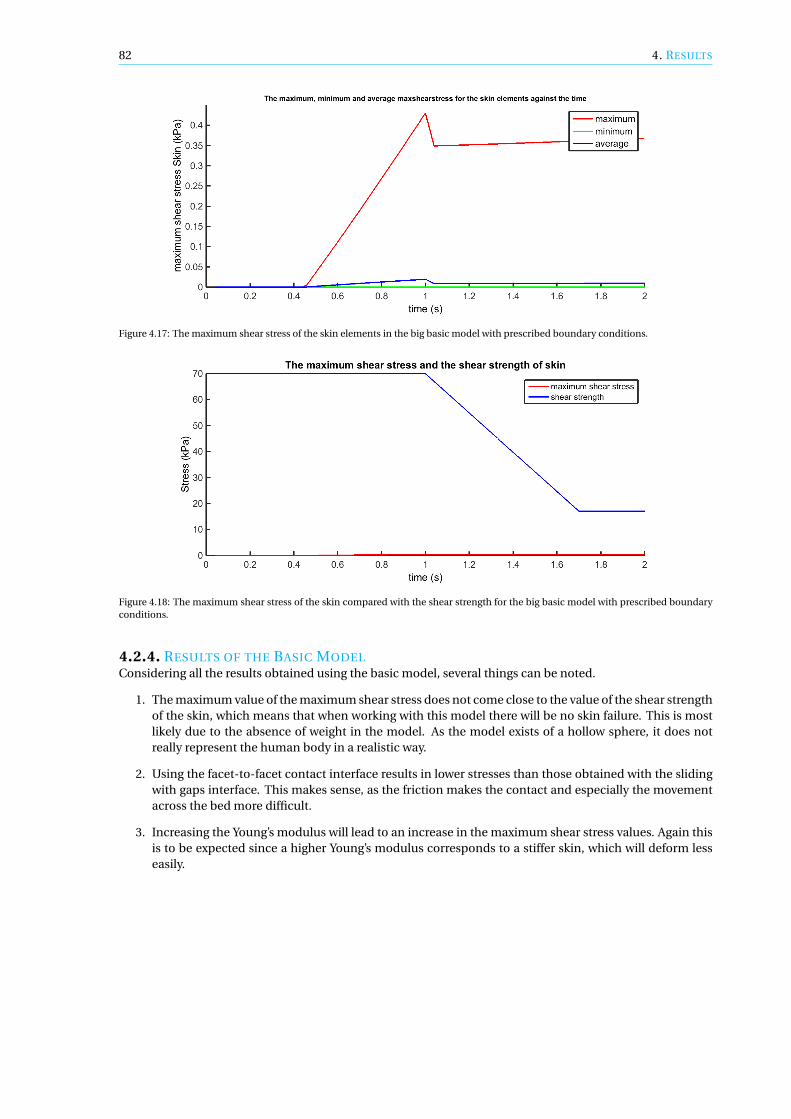
4.16 Deformation results of the big basic model with prescribed boundary conditions. . . . . . . . . . 814.17 The maximum shear stress of the skin elements in the big basic model with prescribed boundary
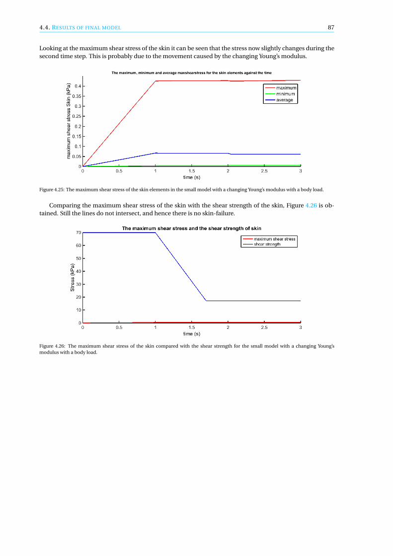
conditions. . . . . . . . . . . . . . . . . . . . . . . . . . . . . . . . . . . . . . . . . . . . . . . . . . . . 824.18 The maximum shear stress of the skin compared with the shear strength for the big basic model
with prescribed boundary conditions. . . . . . . . . . . . . . . . . . . . . . . . . . . . . . . . . . . . 824.19 The coefficient of friction for a skin temperature of Ts = 30C. . . . . . . . . . . . . . . . . . . . . . 834.20 Deformation results of the small model including microclimate factors with a body load. . . . . 844.21 The maximum shear stress of the skin elements in the small model including microclimate fac-
tors with a body load. . . . . . . . . . . . . . . . . . . . . . . . . . . . . . . . . . . . . . . . . . . . . . 844.22 The maximum shear stress of the skin compared with the shear strength for the small model
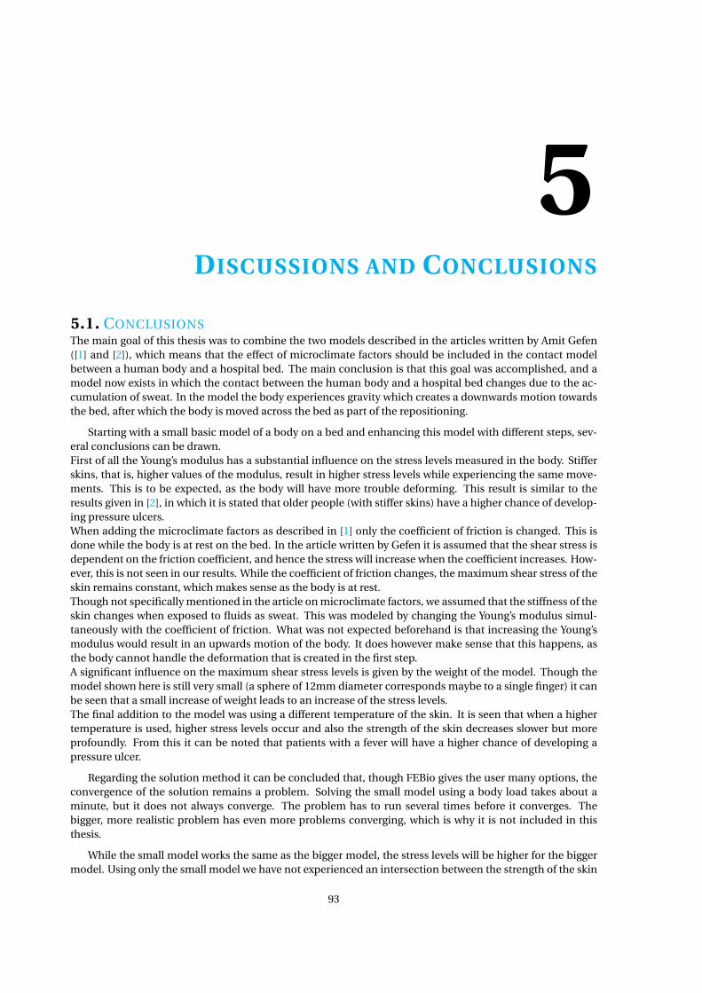
including microclimate factors with a body load. . . . . . . . . . . . . . . . . . . . . . . . . . . . . 854.23 Deformation results of the small model with a changing Young’s modulus with a body load. . . . 864.24 The downward of the small model with a changing Young’s modulus. . . . . . . . . . . . . . . . . 864.25 The maximum shear stress of the skin elements in the small model with a changing Young’s
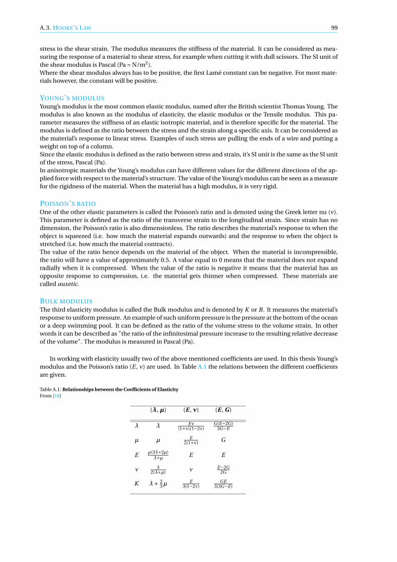
modulus with a body load. . . . . . . . . . . . . . . . . . . . . . . . . . . . . . . . . . . . . . . . . . 874.26 The maximum shear stress of the skin compared with the shear strength for the small model
with a changing Young’s modulus with a body load. . . . . . . . . . . . . . . . . . . . . . . . . . . . 874.27 Deformation results of the small model with additional weight modeled with a body load. . . . . 884.28 The downward of the small model with additional weight. . . . . . . . . . . . . . . . . . . . . . . . 884.29 The maximum shear stress of the skin elements in the small model with additional weight mod-
eled with a body load. . . . . . . . . . . . . . . . . . . . . . . . . . . . . . . . . . . . . . . . . . . . . 894.30 The maximum shear stress of the skin compared with the shear strength for the small model
with additional weight modeled with a body load. . . . . . . . . . . . . . . . . . . . . . . . . . . . . 894.31 The accumulation of perspiration for different skin temperatures. . . . . . . . . . . . . . . . . . . 894.32 The coefficient of friction for different skin temperatures. . . . . . . . . . . . . . . . . . . . . . . . 904.33 The shear strength of the skin for different skin temperatures. . . . . . . . . . . . . . . . . . . . . . 904.34 Deformation results of the small model with Ts = 35C modeled with a body load. . . . . . . . . 904.35 The maximum shear stress of the skin elements in the small model with Ts = 35C modeled with
a body load. . . . . . . . . . . . . . . . . . . . . . . . . . . . . . . . . . . . . . . . . . . . . . . . . . . 914.36 The maximum shear stress of the skin compared with the shear strength for the small model
with Ts = 35C modeled with a body load. . . . . . . . . . . . . . . . . . . . . . . . . . . . . . . . . 914.37 The maximum shear stress of the skin for all different models. . . . . . . . . . . . . . . . . . . . . 92
4.1 Three cases for the small basic model with prescribed boundary conditions. . . . . . . . . . . . . 754.2 A single case for the small basic model with a body load. . . . . . . . . . . . . . . . . . . . . . . . . 784.3 A single case for the big basic model with prescribed boundary conditions. . . . . . . . . . . . . . 814.4 A single case for the small model including microclimate factors with a body load. . . . . . . . . 84
PK1 traction First Piola-Kirchhoff traction vector
PK2 stress Second Piola-Kirchoff stress tensor
BFGS Broyden-Fletcher-Goldfarb-Shanno method
COF Coefficient of Friction
ROI Region of Interest
xi
LIST OF MOST USED SYMBOLS
σ1, σ2, σ3 The principal stresses
τmax Maximum shear stress
F Deformation gradient
X Position in the reference/undeformed configuration
x Position in the current/deformed configuration
φ Mapping between reference and current configuration
J Jacobian (J = det(F))
t(n) Traction vector corresponding to the normal n
σ Cauchy stress tensor
P First Piola-Kirchhoff stress tensor
T First Piola-Kirchhoff traction vector
S Second Piola-Kirchhoff stress tensor
C Right Cauchy-Green deformation tensor
c Eulerian or spatial elasticity tensor
E Green or Lagrangian strain tensor
δW Virtual work
D(. . .)[u] Directional derivative in the direction of u
g Gap function
tT Frictional traction force
µ Coefficient of friction
tN Contact pressure
∆V (t )V The accumulated perspiration over time t within V
Ta Ambient temperature (close to the region of interest)
Ts Skin temperature
τsw Shear strength of the skin
T (x, t ) The temperature at time t and position x
c(x) The specific heat
ρ(x) The mass density
K0 The thermal conductivity
H The heat transfer coefficient
xiii
1INTRODUCTION
Patients that are limited to spending most of their time lying in bed are prone to skin breakdown as a conse-quence of moisture development between the skin and mattress. This wetness results from transpiration orurine. Due to wetting of the skin, the mechanical properties of the skin change and the friction between theskin and the mattress increases. This increase implies that the shear forces at the interface between the skinand mattress increase when a patient is moved or relocated on bed for daily care. This mechanism increasesthe likelihood of the development of a superficial pressure ulcer.
In this research, we will analyze, use and improve the phenomenological model developed by Gefen ([1],[2]) for the simulation of micro-climate factors. This model contains an interaction between the amount oftranspiration, the ambient temperature, the increase of humidity and the increase in the skin-support con-tact pressure. Furthermore, we will analyze and use a finite-element model for the mechanical support andequilibrium of tissue interacting with the mattress where the skin and subcutaneous tissue are incorporated.This interaction poses a contact problem where the surface of contact between the skin and mattress has tobe determined. In this work, we will focus on the combination of the two models, where we aim at predict-ing the likelihood of the development of a superficial pressure ulcer in the course of time upon moving thepatient over the surface of the mattress. This is done by using the finite-element method over the domaincontaining the tissue as well as the mattress. As an output parameter the shear stress will be important toestimate the time at which skin break-down (failure) occurs. Since the mechanical properties of skin changewith local humidity, the skin will deteriorate in the course of time due to the build-up of moisture levels.In this MSc-thesis, we aim at a coupling of the micro-climate factors to the mechanical equilibrium whichconsists of a contact problem.
The basics of this thesis lie in the two articles
• "How do microclimate factors affect the risk for superficial pressure ulcers: A mathematical modelingstudy" by Amit Gefen [1], and
• "Modeling the effects of moisture-related skin-support friction on the risk for superficial pressure ulcersduring patient repositioning in bed" by Eliav Shaked and Amit Gefen [2].
These articles both describe a mathematical model regarding pressure ulcers in bed-bound patients. Thefirst one assesses a patients risk of getting a pressure ulcer. Here a pressure ulcer is said to develop when thestrength of the skin is smaller than the stress obtained by the movement. The second article describes a wayof calculating the shear stress of the skin during movement using the finite element method.
The goal of the thesis can be summarized as follows:
To create a combined model from the two models created by Amit Gefen, in which a patients risk ofpressure ulcers can be assessed when considering not only the contact between the body and the bed,but also including the effects of microclimate factors.
1
2 1. INTRODUCTION
1.1. PRESSURE ULCERSA pressure ulcer is a special type of wound, caused by the appliance of stress on the skin. The official definitionof a pressure ulcer is given by the European Pressure Ulcer Advisory Panel and says the following.
"A pressure ulcer is localized injury to the skin and/or underlying tissue usually over a bonyprominence, as a result of pressure, or pressure in combination with shear. A number of con-tributing or confounding factors are also associated with pressure ulcers; the significance of thesefactors is yet to be elucidated." – http://www.epuap.org
Such a pressure ulcer can occur after a large pressure has been applied to the skin for a short periodof time, or when a small pressure is applied for a long period of time. Pressure ulcers, also referred to as"bedsores" or "pressure sores", usually occur at bony prominences, which are the parts of the body that areusually in direct contact with the underlying surface such as a mattress. Examples of the most commonlocations are the shoulders and the shoulder blades, back of the head, heel, spine and tail bone.
The "European Pressure Ulcer Advisory Panel" (EPUAP) is a panel created to "support all European coun-tries in their efforts to prevent and treat pressure ulcers". The overall mission of this panel is to
" provide the relief of persons suffering from or at risk of pressure ulcers, in particular throughresearch and the education of the public and by influencing pressure ulcer policy in all Euro-pean countries towards an adequate patient centered and cost effective pressure ulcer care." –http://www.epuap.org [3]
In order to improve the communication between the different countries regarding pressure ulcers, theEPUAP has created a "Quick Reference Guide" which has been translated into many different languages. Inthis reference guide guidelines are given that describe how a patients risk of pressure ulcers can be deter-mined, and which factors should be taken into account. In this guide, the different types of pressure ulcersare also divided into four different categories. The categories and their (shortened) explanations are givenbelow. The full explanation can be found on the EPUAP website [3].
Category/Stage I: Non-blanchable erythema Intact skin with non-blanchable redness of a localized areausually over a bony prominence. Darkly pigmented skin may not have visible blanching; its color maydiffer from the surrounding area. The area may be painful, firm, soft, warmer or cooler as compared toadjacent tissue. Category I may be difficult to detect in individuals with dark skin tones. May indicate“at risk” persons.
Category/Stage II: Partial thickness Partial thickness loss of dermis presenting as a shallow open ulcer witha red pink wound bed, without slough. May also present as an intact or open/ruptured serum-filledblister. Presents as a shiny or dry shallow ulcer without slough or bruising where bruising indicatesdeep tissue injury.
Category/Stage III: Full thickness skin loss Full thickness tissue loss. Subcutaneous fat may be visible butbone, tendon or muscle are not exposed. Slough may be present but does not obscure the depth oftissue loss. May include undermining and tunneling.The depth of a Category/Stage III pressure ulcervaries by anatomical location.
Category/Stage IV: Full thickness tissue loss Full thickness tissue loss with exposed bone, tendon or muscle.Slough or eschar may be present. Often includes undermining and tunneling.The depth of a Catego-ry/Stage IV pressure ulcer varies by anatomical location.
As can be seen in the definitions above, these different grades indicate the severity of the injury. In thisthesis the main focus will lie on superficial pressure ulcers. According to Gefen ([1, 2]) these superficial ulcerscorrespond to the pressure ulcers from Grade I and Grade II.
As mentioned in the definition of pressure ulcers, many different factors influence a patients risk at theinjuries. These factors include among others the age of the patient, whether or not the patient is healthy, thewetness of the skin and the stiffness of the skin. Many of these factors are related, for example a patient whohas diabetes often has a stiffer skin.A lot of research has been done and is being done to investigate these factors and decrease patients risk at
1.1. PRESSURE ULCERS 3
pressure ulcers. The models that are described in the articles that will be used in this thesis investigate therelation between the wetness of the skin (microclimate factors) and the risk of pressure ulcers. In the articlesit is described that the temperature in the room has effect on the moisture level of the skin which has effecton the stiffness of the skin, hence again the factors are related.
1.1.1. SKIN BREAKDOWNTo minimize a patients risk at pressure ulcers it is important to know when pressure ulcers develop. A verysimple way of looking at the development of these wounds is to look at it as the skin "failing" or breakingdown. There are multiple theories on the failing of materials, depending on the types of these materials.
A solid material is called ductile when it has the ability to deform under tensile stress, for example whensliding along a different plane. Criteria used to predict the failure of these materials are also known as yieldcriteria. These criteria can be seen as defining the limit of elasticity in a material after which plastic defor-mation will occur. This means that some of the deformations will remain when the material is unloaded.The yield criteria try to ascertain the yield point at which the elastic region, in which unloading the materialmeans the deformations are completely reversed, changes into the plastic region. Note that despite the quicktransition from elastic to plastic behavior, in reality there is no distinct yield point due to continuity ([4]).
Figure 1.1: Schematic representation of a stress-strain diagram for many metals and non-metals. The transition from elastic to plasticbehavior is fast but continuous and can therefore not truly be given by a single yield point. Source: [4]
Note that even though the definition of the yield point does not include actual failing of the material, itis the point at which permanent deformation occurs. In the context of the human body this will therefore beused as the failing point.
Below two of the most common yield criteria will be discussed ([5], [6]).
Maximum shear stress theory Also known as the Tresca yield criterion. This theory states that the materialyields when the maximum shear stress τ exceeds the shear yield strength τy . For the principal stressesordered as σ1 ≥ σ2 ≥ σ3 the maximum shear stress is given equal to 1
2 (σ1 −σ3) (see Sections 2.1.5 and2.1.6). The yield point can hence be determined by solving equation (1.1):
τ= 1
2(σ1 −σ3) = τy . (1.1)
Maximum distortion energy criterion Also known as the von Mises Criterion. This criterion states that fail-ure occurs when the von Mises stress squared σv exceeds the yield strength σy squared. Determiningthe yield point can be done by solving equation (1.2) where σ1, σ2 and σ3 are the principal stresses, i.e.
σ2v = 1
2[(σ1 −σ2)2 + (σ1 −σ3)2 + (σ2 −σ3)2] =σ2
y . (1.2)
In this thesis the Maximum shear stress theory shall be used as this theory is also described by Gefen in[1]. In the article Gefen uses this theory to determine the critical time point for skin breakdown t∗ which is infact the time when the yield point is reached (see Figure 1.2). In Section 4.1.1 a more detailed explanation ofthe use of the Maximum shear stress theory in this thesis is given.
4 1. INTRODUCTION
Figure 1.2: Skin break down will occur when the shear stress applied on the skin exceeds the shear strength of the skin. Source: [1]
1.2. PREVIOUS RESEARCHThis section will discuss the article on the effects of microclimate factors on the development of pressureulcers written by Gefen [1] and the research that was done in the beginning of this thesis regarding the mostsuitable software.
1.2.1. THE EFFECTS OF THE MICRO CLIMATEThe paper by Amit Gefen [1] reviews a mathematical model which describes the effect of microclimate factorson the development of pressure ulcers.In this section the assumptions, calculations and results of this article will be discussed.
In the article the risk of superficial pressure ulcers (SPUs) is being examined. Here superficial pressureulcers will mean "skin damage associated with sustained mechanical loading".The research described in the article continues on the idea that thermodynamic conditions within and aroundthe skin tissue (i.e. the skin being wet) influences the risk of a patient getting a SPU. The term microclimateis used here to describe factors like the local temperature and moisture conditions of the skin. The area ofinterest will be the parts of the human body that are considered the weight-bearing regions ([7]1). Previouspapers described the effect of surface temperature, humidity, moisture and air movement as risk factors onthe patients susceptibility. All these papers however, were based on purely experimental research. The articlewritten by Gefen creates a mathematical model to prove that the microclimate factors are indeed risk factors.
In Figure 1.3 the part of the human body that is considered is shown. This region of interest (ROI) is "asmall region of contact between the skin and a support (e.g. mattress or cushion), possibly with a coveringsheet, some clothing or stocking in-between the skin and support".
Figure 1.3: The model will consider a small weight-bearing part of the human body. Source: [1]
1Referred to by Gefen in [1].
1.2. PREVIOUS RESEARCH 5
Perspiration The first step that is taken in the article is to assume the expression of the perspiration accu-mulated over a certain time period within the available space.The following denotations are used.
Notation Factor
∆V volume of perspiration
t time
V available space between the skin and the contact materials at the ROI
S rate of production of perspiration by the sweat glands contained on the ROI
D rate of drainage of perspiration out of the ROI via the contact materials
E rate of evaporation of perspiration.
With the factors above, the accumulated perspiration over time t within V is assumed to be
∆V (t )
V=
t∫0
(S − E − D)d t (1.3)
Now the rate of production of perspiration can be assumed to start with an ambient temperature Ta (tem-perature within the ROI) of 30C. It can also be assumed that the production is proportional to the tempera-ture gradient Ta −30C. Using this S can be formulated as
S =α Ta −30C
T maxa −T min
s. (1.4)
Here α is a dimensionless proportionality constant, T maxa is the maximal ambient temperature and is equal
to 40C and T mins is the minimal skin temperature, equal to 30C.
In a similar way the evaporation rate is formulated.
E =β Ta −Ts
T maxa −T min
s(1−RH) (1.5)
Here β is another dimensionless proportionality constant, Ts is the skin temperature and RH is the relativehumidity at the liquid free-space of the ROI. In the article a more detailed definition is given.
"The RH is defined as the ratio between the amount of water vapor at the ROI and the maximumamount of water vapor that the ROI can hold, and hence, the RH ranges between 0 and 1." - AmitGefen, [1]
With this definition it can be noted that RH = 1− ∆V (t )V . In the paper, however, Gefen mentions but does not
use this definition; RH is simply assumed constant2.Lastly an expression for the drainage of perspiration D is given. This is simply given as a single dimen-
This constant weighs together the contributions of permeabilities of all contact materials. If for instanceγ= 0, there is no drainage of perspiration at all.
To establish a model that is, mathematically speaking, simple enough to solve, the assumption is madethat the ambient temperature, skin temperature and relative humidity do not change in time, and thus areindependent of t . With these assumptions and using equations (1.4), (1.5) and (1.6) equation (1.3) becomes
2Note that when RH = 1− ∆V (t )V would be used equation (1.5) would simplify to
E =β Ta −Ts
T maxa −T min
s
∆V (t )
V
and equation (1.3) could be solved exact.
6 1. INTRODUCTION
∆V (t )
V=
[α
Ta −30C
T maxa −T min
s+β Ta −Ts
T maxa −T min
s(1−RH)+γ
]· t , (1.7)
with t such that 0 ≤∆V (t )/V ≤ 1.
The coefficient of friction Another factor in the model described in the article is the coefficient of friction(COF) between the skin and a contacting covering sheet or clothing. This coefficient strongly depends on thevolume of perspiration accumulated over the skin.For instance, for the contact between dry skin and common hospital textiles the COF is equal to approxi-mately 0.4. For contact between wet skin and the same textiles the COF will increase to approximately 0.9.Using this, an expression for the COF (denoted as µ) between the skin and the covering sheet or clothing inthe ROI is described for the model;
µ= 0.5∆V (t )
V+0.4. (1.8)
This equation shows that the accumulation of perspiration on the skin will consequently increase the shearforces f between the skin and the contact materials over time.For the shear forces f it holds that f = µN where N is the body weight force applied perpendicularly to theskin-support or skin-clothing contact area at the weight-bearing region. This body weight force N is assumedto be constant over time since the patient is not moving. Despite this fact, µ does increase with time as can beobtained from equation (1.8). As a consequence the shear stress between the skin and the contact materialswill increase over time, as the amount of perspiration increases. This shear stress τ is equal to the shear forcenormalized by the contact area A which gives τ = µN /A. Because the pressure P delivered to the skin fromthe support surface at the skin-support or clothing-support region of contact is given as P = N /A the shearstress can be written in terms of this pressure, that is τ=µP . Substituting the expression of the COF (equation(1.8) into this relationship the following equation holds for the ROI.
τ=(0.5∆V (t )
V+0.4
)·P (1.9)
Here the pressure P depends on the stiffness of the support, and will increase as the stiffness of the supportincreases ([8]3). Since τ is linearly proportional to P , the same dependency on the stiffness of the support willhold.
Skin Breakdown When the shear stress applies on the skin (given by equation (1.9)) exceeds the shearstrength of the skin, skin break down will occur (Figure 1.4). It was shown before that the shear stress willincrease over time as perspiration accumulates. The shear strength of the skin will however decline. A refer-ence is given to ([9]) regarding the fact that the shear strength reduces "by a factor 5 for a completely hydratedskin with respect to dry skin." Using this an expression of the shear strength of the skin τs
w is given.
τsw =
(1−0.8
∆V (t )
V
)τs
0 (1.10)
Here τs0 is the shear strength of dry skin.
Since the skin breaks down when the shear stress applied on the skin exceeds the shear strength of theskin, the next step is to find the time t∗ for which the shear stress is equal to the shear strength of the skin,hence where τ= τs
w . This equality yields
t∗ = τs0 −0.4P
(0.5P +0.8τs0)
[α−β(1−RH)]Ta+β(1−RH)Ts−α·30C
T maxa −T min
s−γ
(1.11)
With this equation it is possible to examine the effect of the different factors on this critical time t∗.
3Referred to by Gefen in [1].
1.2. PREVIOUS RESEARCH 7
Figure 1.4: Skin break down will occur when the shear stress applied on the skin exceeds the shear strength of the skin. Source: [1]
CALCULATIONS
In the article, the effect of the microclimate factors Ta , RH and Ts as well as interacting factors P and per-meability γ on the critical time for skin breakdown is examined. In order to study the effects of these factorson the critical time, several plots were made in which the factors were given various values. In every plot, thecritical time (t∗) is plotted against the skin temperature (Ts ) and one of the other factors is being varied. InTable 1.1 the values for all parameters are given. Note that whenever one of the factors is being varied, theothers are equal to the values given in this table [1].The Matlab code used to repeat the calculations can be found in Appendix (C.1).
Table 1.1: These parameter values are used in the plots shown in Figure 1.5 .
Parameters τs0 P α β γ Ta RH
Value 70 kPa 7 kPa 2 1 0.1 35C 0.5
RESULTS
In the article the results are given using the plots shown in Figure 1.5. It can be seen in the figures that all thefactors which have been examined do have effect on the critical time.
8 1. INTRODUCTION
Figure 1.5: The calculated dimensionless critical times for skin breakdown versus the skin temperature (Ts ) for different values of (a)the microclimate parameters of ambient temperature (Ta ) (left panel) and relative humidity (RH) (right panel), and (b) the interact-ing parameters of pressure delivered from the support (P ) (left panel) and permeability to perspiration (γ) of the materials contact-ing the skin or being in close proximity to the skin (right panel). The following values were assigned to the model variables in thesesimulations:τs
0 = 70 kPa, P = 7 kPa∗, α = 2, β = 1, and γ = 0.13, Ta = 35C∗ and RH = 0.53. ∗ denotes; where not altered as detailed inthe specific panel. Source: [1]
1.2.2. CHOOSING A SOFTWARE PACKAGEIn this thesis the goal is to combine the two models regarding pressure ulcers created by Gefen ([1], [2]). Asone of the models uses the finite element method to solve the problem, a suitable software package had tobe found. This software needs to be widely accessible and easy to change, that is, it should be possible to addfeatures such as the effect of microclimate factors. The second model of Gefen originally was implementedusing software called Adina ([10]), hence the first software we checked was Adina.
ADINA - FINITE ELEMENT ANALYSIS SOFTWARE
The software package called Adina ([10]) allows the user to model 2D problems which are solved using FiniteElement Methods. It has a graphic interface hence the user does not need any programming skills.To be able to fully use the software it needs to be purchased. A free trial version can be obtained4 but whenusing this version the number of nodes is limited to 900.As the software is not open source the user does not have the opportunity to obtain details regarding the cal-culations from the code. Using Adina the user is obligated to buy the full version, but even when purchasedis limited to working with 2D problems in a graphic interface, unable to combine the model with other math-ematical models. Due to these limitations we decided to look at other software packages and discard the useof Adina.
FEBIO
FEBio ([11]) is software constructed to solve medical problems using a Finite Element Analysis. The softwareis open source and is created by the University of Utah using C++. The software is originally constructedtogether with two other programs; PreView ([12]) and PostView ([13]).
PreView Also constructed by the University of Utah, PreView is the original predecessor of FEBio. Quitesimilar to Adina, the problem can be modeled using a graphical interface. Opposite to Adina, FEBio is onlycapable to solve problems in 3D.
4The trial version can be downloaded at http://www.adina.com/n900.shtml.
1.2. PREVIOUS RESEARCH 9
(a) Opening Adina the user is presented with manyoptions.
(b) When building a model in the trial version theuser is limited to 900 nodes.
Figure 1.6: The software package Adina.
In PreView the user has to implement the geometries, boundary conditions, types of contact and so on.Since PreView can only build basic geometries it is possible to import more advanced geometries built usingother software. Besides information regarding the problem, various details about solving the problem can bedefined in PreView. Examples of these details are the maximum number of retries for each time step and thesolution method.Once the model is complete a FEBIO (.feb) file is made, which can be run using FEBio.
(a) The basic screen of PreView. (b) Simple geometries can be created in PreView.
Figure 1.7: The predecessor PreView.
FEBio Once the .feb file has been generated the user can run this file in FEBio which solves the modeledproblem. On Windows the program can be run directly from PreView, from a command prompt or from thePrograms Menu. In running FEBio the user will see a command prompt on the screen which shows the detailsof every time step (see Figure 1.8). When finished solving the problem FEBio will simply stop and the outputwill be saved in several files.
Figure 1.8: FEBio while solving a problem.
10 1. INTRODUCTION
PostView Once the problem is solved using FEBio, the output can be viewed in the post processor PostView.In this program the user can view different outputs such as the stresses, strains and deformations of the bod-ies at every time step. Similar to Adina, the package consisting of FEBio, PreView and PostView is very graphic.
(a) Showing the stress results using PostView. (b) Showing results for a specific element usingPostView
Figure 1.9: PostView can be used to view many different outputs.
The user can implement the model by choosing the correct settings. As the package exists of three differentprograms, the user also has the opportunity to choose a different method for creating the .feb file. The userfor example can write the file manually using the XML language. This opportunity is very convenient becauseit means we could use a mathematical program such as Matlab to write the .feb file and to add the effects ofmicro-climate factors such as sweat.Another advantage of FEBio is that the software is open source, it is therefore possible to view and evenchange the source code.
MATLAB
The goal in this thesis is to combine two mathematical models. Working with mathematical models the mostcommon first computational environment to use is Matlab. Since Matlab allows the user to implement math-ematical models in which functions can be called, Matlab is very suitable to model the micro-climate factorsfor a bedbound patient. However, since Matlab itself does not have a Finite Element Solver for large prob-lems, this solver would have to be implemented separately which would be very time consuming.As FEBio is a Finite Element solver in which Bio-mechanical problems can be solved and Matlab is a programin which the micro-climate factors can be modeled, it would be very convenient if we could combine thesetwo programs.
THE GIBBON TOOLBOX
When further investigating the possibilities of FEBio combined with Matlab, we came across the Gibbon Tool-box ([14]). This is a set of Matlab codes in which a problem is modeled, a FEBio file is created, FEBio is calledto solve the problem, and which then shows the user specified output. Basically this toolbox allows the userto replace PreView (and PostView) with Matlab, but still use FEBio to actually solve the problem.
THE FINAL SOFTWARE CHOICE
Using the information described above a final choice for the software was made. Instead of choosing a singleprogram the choice was made to use the combination of Matlab, the Gibbon Toolbox and FEBio. Using Matlaband the Gibbon Toolbox a .feb file will be generated in which the problem including the micro-climate factorswill be described. When completely defined, the model will then be solved using FEBio. Once solved, theresults will be viewed using either Matlab, PostView or a combination. A schematic overview of this can beseen in Figure 1.10.Note that this section does not cover all possible software packages. Other programs, such as Abaqus ([15])
have not been considered in the choice because they are quite similar to FEBio and Adina.
1.3. OUTLINE OF THIS THESIS 11
Figure 1.10: A schematic overview of the chosen software. The logos were retrieved from [14], [11]and [13]
1.3. OUTLINE OF THIS THESISThis document is organized in the following chapters:
• Chapter 2 describes the mathematical model that is solved in this thesis. In the final sections the im-plementation of the model in the software is discussed.
• Chapter 3 gives the details on the numerical method that is used to solve the problem.
• Chapter 4 is subdivided into three sections, each discussing the results obtained with a part of themodel. The first section discusses the basic model, the second section discusses the results of themodel in which microclimate factors are included. The last section discusses the final model whichis enhanced with the improvements discussed in Chapter 2.4.3.
• Chapter 5 includes the conclusions, remarks and ideas concerning future research.
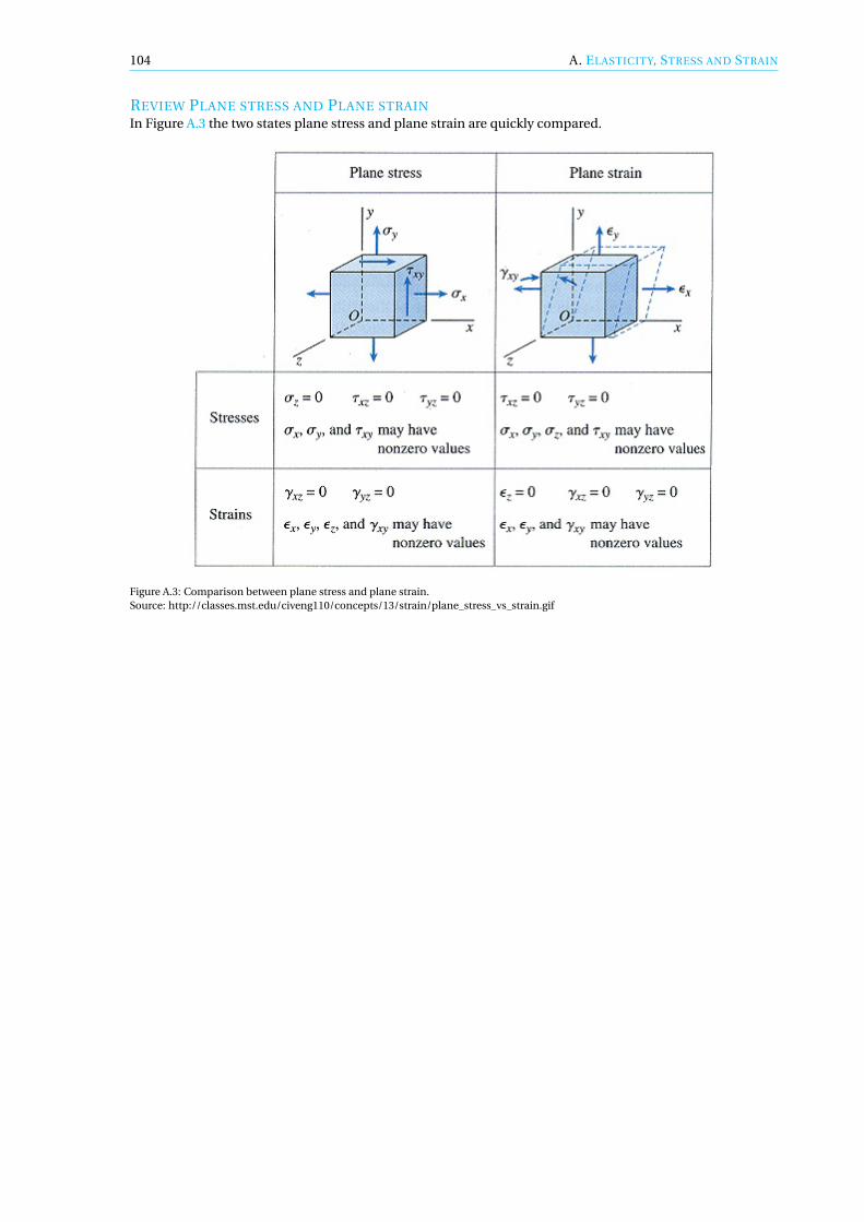
• Appendix A gives additional information regarding stress and strain, as well as some information re-garding constitutive laws such as Hooke’s Law.
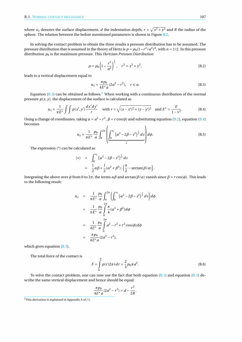
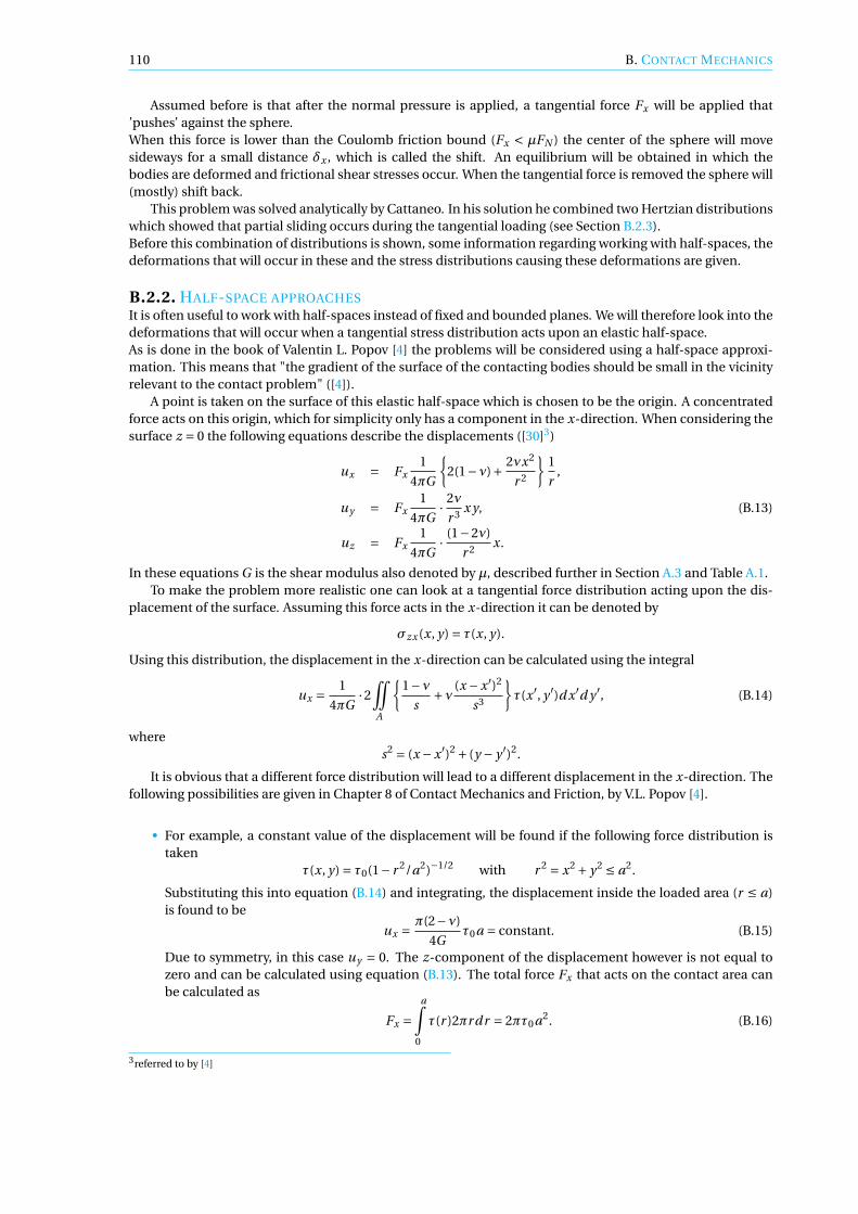
• Appendix B provides additional information on contact mechanics. Different solving methods are de-scribed.
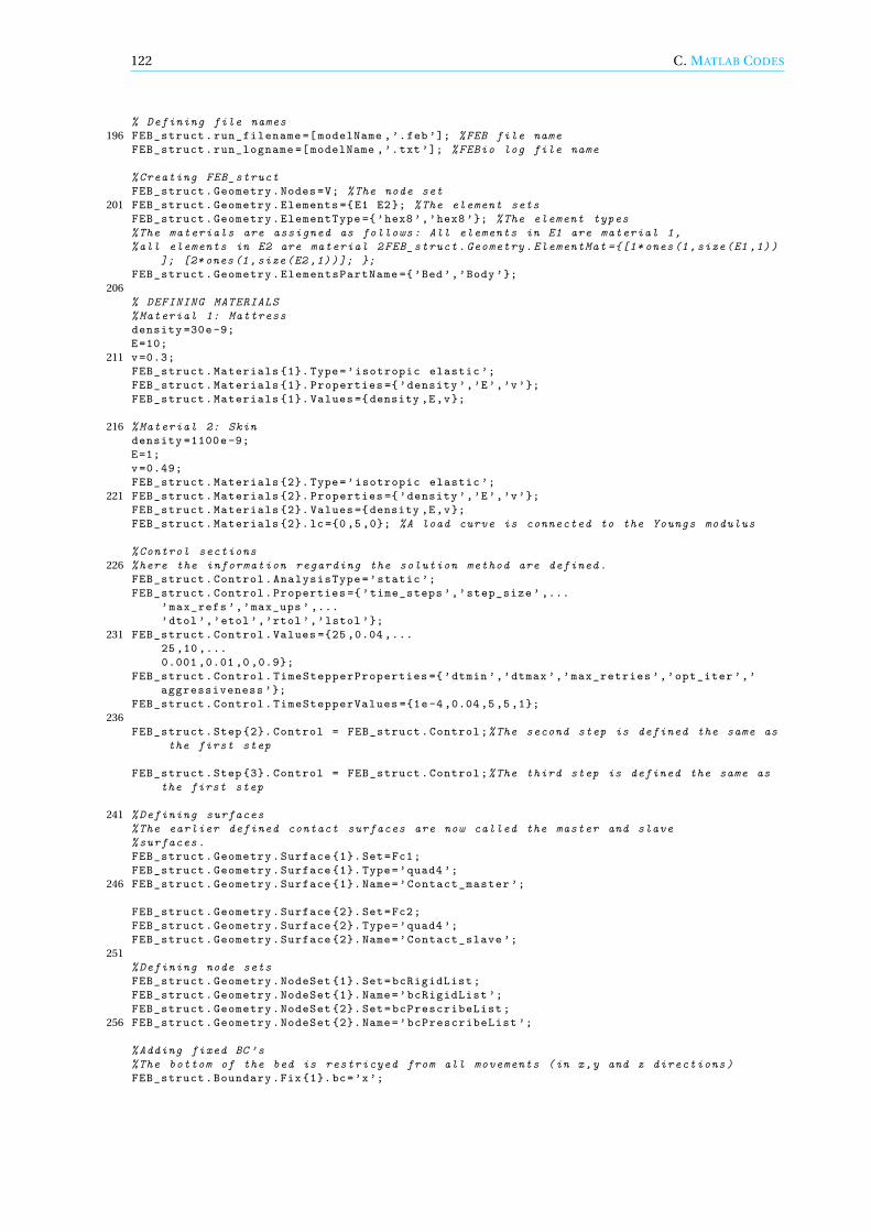
• Appendix C contains the Matlab code of the final model.
• Appendix D contains the FEBio file of the final model.
2MATHEMATICAL MODEL
In this chapter the mathematical model will be discussed. The first section will contain the necessary def-initions regarding stress and deformation. In the second section (Section 2.2) the problem will be given inmathematical equations. The section will start with discussing the basic principles of mechanics, after whichthe actual problem will be derived. Section 2.3 will then elaborate on the mathematical model by includ-ing the contact information. Lastly, Section 2.4 explains the model as it is constructed using the software. Itshould be noted that Sections 2.2 and 2.3 give the mathematical problem as implemented in FEBio, whereasSection 2.4 only provides the details that are needed to solve the model.
2.1. DEFORMATION AND STRESSIn contact between solids and the deformation of solids the concepts of elasticity, stress and strain are veryimportant. In the subject of pressure ulcers, stress especially is important. In this section mostly deformationand stress will be discussed. More information on elasticity, stress and strain is provided in Appendix A. Theknowledge used in this section and its subsections is acquired a.o. from the books Theory of Elasticity, byS. Timoshenko and J.N. Goodier [16], Nonlinear Continuum Mechanics for Finite Element Analysis by JavierBonet and Richard D. Wood [17], and Introduction to Finite Element Analysis Using MATLAB rand Abaqusby Amar Khennane, chapter 5 [18]. More information on stress and strain can be found in Appendix A.
2.1.1. THE DEFORMATION GRADIENTWhen considering a deforming body one has a reference configuration (the undeformed body) and a currentconfiguration (the deformed body). During the deformation many quantities can change such as the area ofa part of the body, the volume, and even the density. This is illustrated in Figure 2.1.
To be able to link the quantities of the reference configuration to the quantities of the current deformation(or even during the deformation) the deformation gradient F is introduced. This tensor makes it possible todescribe the relative spatial position of of two neighboring particles after deformation in terms of their relativematerial position before deformation.
When the motion of the deformable body at time t is described by a mapping x = φ(X, t ) between theinitial positions denoted by X and the current positions denoted by x, the deformation gradient is defined as
F = ∂φ
∂X=∇φ. (2.1)
Note that hereφ is a vector and hence F is a matrix.This definition is derived from the following idea. Consider a material particle P in the reference config-
uration and a material particle Q1 in the neighborhood of P . The position of Q1 relative to P is given by theelemental vector dX1.
dX1 = XQ1 −XP (2.2)
After the body is deformed, both Q1 and P will have deformed to spatial positions given by
xp = φ(XP , t ) (2.3a)
xq1 = φ(XQ1 , t ). (2.3b)
13
14 2. MATHEMATICAL MODEL
Figure 2.1: Many quantities change in the deformation of a body. Source: [17]
Applying the deformation and using equation (2.2) the elemental vector becomes
dx1 = xq1 −xp =φ(XP +dX1, t )−φ(XP , t ). (2.4)
Using the definition of F and assuming ‖dX1‖ to be sufficiently small, this can be rewritten as
dx1 = FdX1. (2.5)
Note that the motion of the deformable body can also be expressed as
x = x(X, t ). (2.6)
In this case the deformation gradient is given by
F = ∂x
∂X. (2.7)
When considering only a single elemental material vector dX, the corresponding vector dx in the deformed(spatial) configuration is given by
dx = FdX. (2.8)
The inverse of the deformation gradient can be used to express the reference position of a particle in terms ofthe position in the current configuration. The inverse is given by
F−1 = ∂X
∂x=∇φ−1. (2.9)
CHANGE IN VOLUME
The deformation gradient can be used to express many quantities, among which is the change in volumewhen a body deforms [17]. Consider an infinitesimal vector element in the material (reference) configurationdefined by the following three edges (see Figure 2.2).
dX1 = d X1E1 (2.10a)
dX2 = d X2E2 (2.10b)
dX3 = d X3E3 (2.10c)
Here E1, E2 and E3 are the orthogonal unit vectors which means that the edges of the volume element areparallel to the Cartesian axes.
2.1. DEFORMATION AND STRESS 15
Figure 2.2: The volume change of an element caused by the deformation of a body. Source: [17]
The elemental material volume is obviously given by
dV = d X1d X2d X3. (2.11)
The deformed volume can be derived by first considering the spatial vectors that define the element in thespatial configuration.
dx1 = FdX1 = ∂φ
∂X1d X1 (2.12a)
dx2 = FdX2 = ∂φ
∂X2d X2 (2.12b)
dx3 = FdX3 = ∂φ
∂X3d X3 (2.12c)
Using these elemental vectors the deformed volume is given by
d v = |dx1 · (dx2 ×dx3)|= | ∂φ
∂X1· (∂φ
∂X2× ∂φ
∂X3)d X1d X2d X3| (2.13)
It can be noted that the triple product in equation (2.13) is the determinant of the deformation gradient F.Using this the volume change caused by deformation can be expressed using the Jacobian J .
d v = JdV , J = detF (2.14)
This expression will be used later on in this section.
2.1.2. PUSH FORWARD AND PULL BACKIn the previous section the deformation gradient is introduced as the relationship between the undeformed(material) and deformed (spatial) quantities. Many studies in literature however, use the concepts of pushforward and pull back to express these relationships.
Push forward is used to express the spatial form in terms of the material form. For example, the elementalvector dx is the push forward equivalent of the material vector dX, which is expressed as
dx =φ∗ [dX] = FdX. (2.15)
16 2. MATHEMATICAL MODEL
Pull back is used to express the material form in terms of the spatial form. Taking the same example, thematerial vector dX is the pull back equivalent of the spatial vector dx, expressed as
dX =φ−1∗ [dx] = F−1dX. (2.16)
Note thatφ∗ denotes an operation, which is evaluated differently for different operands [] [17].
2.1.3. THE STRESS TENSORIf one applies pressure or other external forces on the outside of an object and this object is being restrainedagainst rigid body movement, this pressure will be noted inside the object as internal forces are induced.These internal forces have a certain intensity, i.e. a certain amount of force per unit area of the surface onwhich they act. This intensity of the internal forces is called stress. The dimension of stress is pressure, henceit is mostly measured in terms of pascal (Pa).
THE CAUCHY STRESS TENSOR
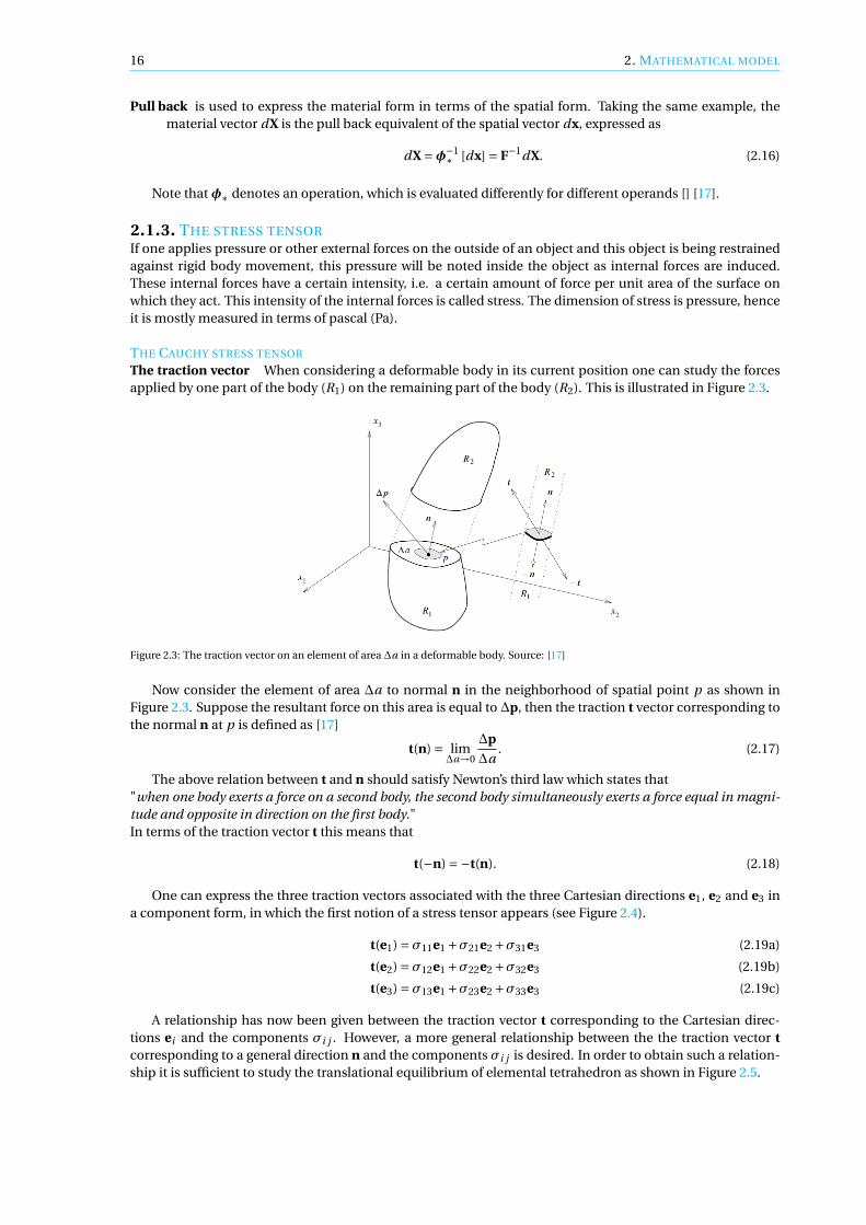
The traction vector When considering a deformable body in its current position one can study the forcesapplied by one part of the body (R1) on the remaining part of the body (R2). This is illustrated in Figure 2.3.
Figure 2.3: The traction vector on an element of area ∆a in a deformable body. Source: [17]
Now consider the element of area ∆a to normal n in the neighborhood of spatial point p as shown inFigure 2.3. Suppose the resultant force on this area is equal to ∆p, then the traction t vector corresponding tothe normal n at p is defined as [17]
t(n) = lim∆a→0
∆p
∆a. (2.17)
The above relation between t and n should satisfy Newton’s third law which states that"when one body exerts a force on a second body, the second body simultaneously exerts a force equal in magni-tude and opposite in direction on the first body."In terms of the traction vector t this means that
t(−n) =−t(n). (2.18)
One can express the three traction vectors associated with the three Cartesian directions e1, e2 and e3 ina component form, in which the first notion of a stress tensor appears (see Figure 2.4).
t(e1) =σ11e1 +σ21e2 +σ31e3 (2.19a)
t(e2) =σ12e1 +σ22e2 +σ32e3 (2.19b)
t(e3) =σ13e1 +σ23e2 +σ33e3 (2.19c)
A relationship has now been given between the traction vector t corresponding to the Cartesian direc-tions ei and the components σi j . However, a more general relationship between the the traction vector tcorresponding to a general direction n and the components σi j is desired. In order to obtain such a relation-ship it is sufficient to study the translational equilibrium of elemental tetrahedron as shown in Figure 2.5.
2.1. DEFORMATION AND STRESS 17
Figure 2.4: It is possible to express the traction vectors in a component form, introducing the notion of a stress tensor. Source: [17]
Figure 2.5: Considering the translational equilibrium of an elemental tetrahedron one can obtain a relationship between the tractionvector t corresponding to a general direction n and the components σi j . Source: [17]
Taking f to be the force per unit volume acting on the body at point p, the equilibrium of the tetrahedronis given as
t(n)d a +3∑
i=1t(−ei )d ai + fd v = 0. (2.20)
In this equation d ai = (n ·ei )d a is the projection of the area d a onto the plane orthogonal to the Cartesiandirection i and d v is the volume of the tetrahedron. This expression can be rewritten by dividing the equationby d a, using Newton’s third law and equations (2.19a)–(2.19c) and noting that d v/d a → 0.
t(n) = −3∑
j=1t(−e j )
d a j
d a− f
d v
d a
=3∑
j=1t(e j )(n ·e j )
=3∑
i , j=1σi j (e) (2.21)
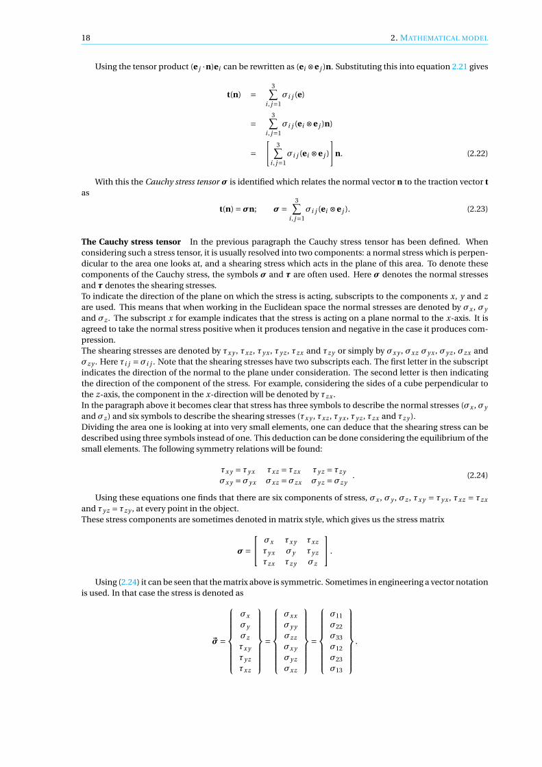
18 2. MATHEMATICAL MODEL
Using the tensor product (e j ·n)ei can be rewritten as (ei ⊗e j )n. Substituting this into equation 2.21 gives
t(n) =3∑
i , j=1σi j (e)
=3∑
i , j=1σi j (ei ⊗e j )n)
=[
3∑i , j=1
σi j (ei ⊗e j )
]n. (2.22)
With this the Cauchy stress tensor σ is identified which relates the normal vector n to the traction vector tas
t(n) =σn; σ=3∑
i , j=1σi j (ei ⊗e j ). (2.23)
The Cauchy stress tensor In the previous paragraph the Cauchy stress tensor has been defined. Whenconsidering such a stress tensor, it is usually resolved into two components: a normal stress which is perpen-dicular to the area one looks at, and a shearing stress which acts in the plane of this area. To denote thesecomponents of the Cauchy stress, the symbols σ and τ are often used. Here σ denotes the normal stressesand τ denotes the shearing stresses.To indicate the direction of the plane on which the stress is acting, subscripts to the components x, y and zare used. This means that when working in the Euclidean space the normal stresses are denoted by σx , σy
and σz . The subscript x for example indicates that the stress is acting on a plane normal to the x-axis. It isagreed to take the normal stress positive when it produces tension and negative in the case it produces com-pression.The shearing stresses are denoted by τx y , τxz , τy x , τy z , τzx and τz y or simply by σx y , σxz σy x , σy z , σzx andσz y . Here τi j =σi j . Note that the shearing stresses have two subscripts each. The first letter in the subscriptindicates the direction of the normal to the plane under consideration. The second letter is then indicatingthe direction of the component of the stress. For example, considering the sides of a cube perpendicular tothe z-axis, the component in the x-direction will be denoted by τzx .In the paragraph above it becomes clear that stress has three symbols to describe the normal stresses (σx , σy
and σz ) and six symbols to describe the shearing stresses (τx y , τxz , τy x , τy z , τzx and τz y ).Dividing the area one is looking at into very small elements, one can deduce that the shearing stress can bedescribed using three symbols instead of one. This deduction can be done considering the equilibrium of thesmall elements. The following symmetry relations will be found:
τx y = τy x τxz = τzx τy z = τz y
σx y =σy x σxz =σzx σy z =σz y. (2.24)
Using these equations one finds that there are six components of stress, σx , σy , σz , τx y = τy x , τxz = τzx
and τy z = τz y , at every point in the object.These stress components are sometimes denoted in matrix style, which gives us the stress matrix
σ= σx τx y τxz
τy x σy τy z
τzx τz y σz
.
Using (2.24) it can be seen that the matrix above is symmetric. Sometimes in engineering a vector notationis used. In that case the stress is denoted as
~σ=
σx
σy
σz
τx y
τy z
τxz
=
σxx
σy y
σzz
σx y
σy z
σxz
=
σ11
σ22
σ33
σ12
σ23
σ13
.
2.1. DEFORMATION AND STRESS 19
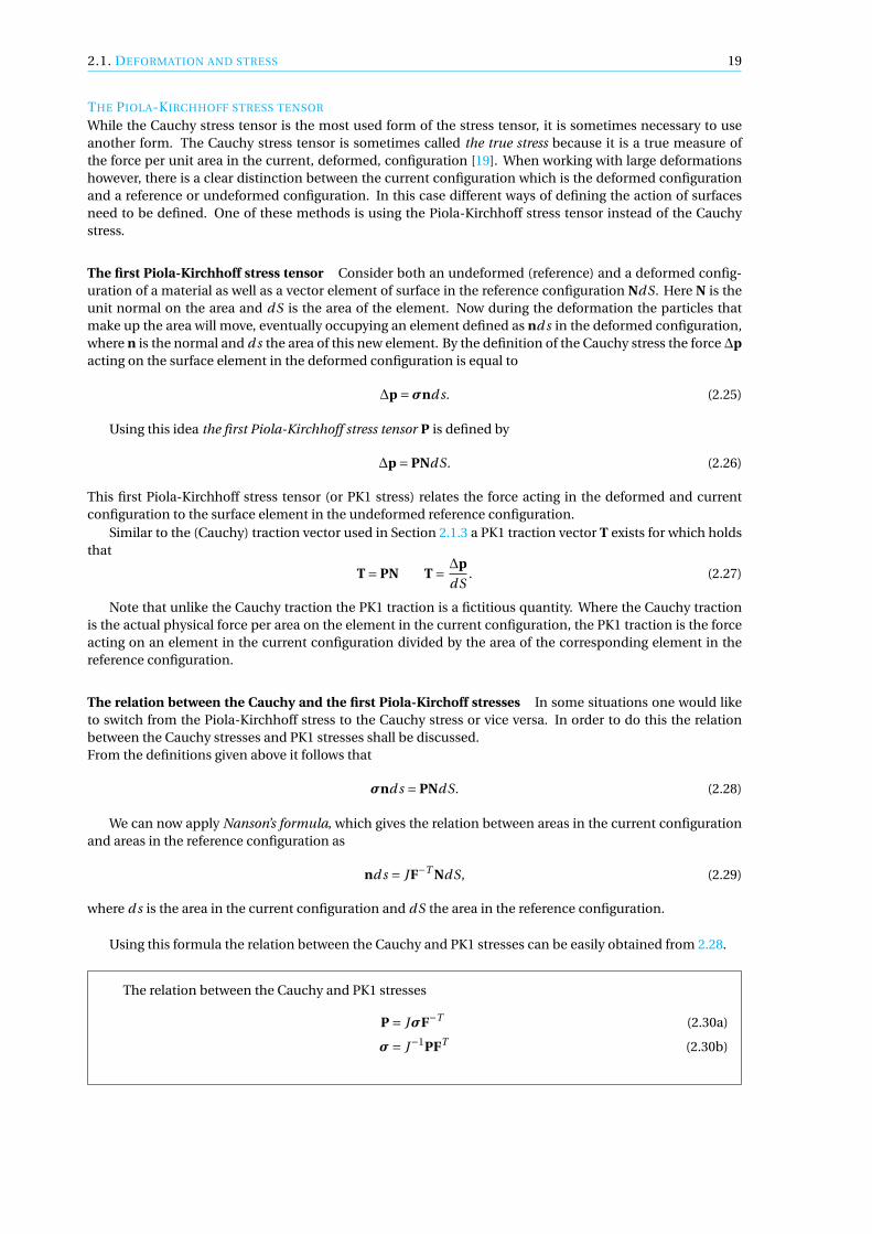
THE PIOLA-KIRCHHOFF STRESS TENSOR
While the Cauchy stress tensor is the most used form of the stress tensor, it is sometimes necessary to useanother form. The Cauchy stress tensor is sometimes called the true stress because it is a true measure ofthe force per unit area in the current, deformed, configuration [19]. When working with large deformationshowever, there is a clear distinction between the current configuration which is the deformed configurationand a reference or undeformed configuration. In this case different ways of defining the action of surfacesneed to be defined. One of these methods is using the Piola-Kirchhoff stress tensor instead of the Cauchystress.
The first Piola-Kirchhoff stress tensor Consider both an undeformed (reference) and a deformed config-uration of a material as well as a vector element of surface in the reference configuration NdS. Here N is theunit normal on the area and dS is the area of the element. Now during the deformation the particles thatmake up the area will move, eventually occupying an element defined as nd s in the deformed configuration,where n is the normal and d s the area of this new element. By the definition of the Cauchy stress the force∆pacting on the surface element in the deformed configuration is equal to
∆p =σnd s. (2.25)
Using this idea the first Piola-Kirchhoff stress tensor P is defined by
∆p = PNdS. (2.26)
This first Piola-Kirchhoff stress tensor (or PK1 stress) relates the force acting in the deformed and currentconfiguration to the surface element in the undeformed reference configuration.
Similar to the (Cauchy) traction vector used in Section 2.1.3 a PK1 traction vector T exists for which holdsthat
T = PN T = ∆p
dS. (2.27)
Note that unlike the Cauchy traction the PK1 traction is a fictitious quantity. Where the Cauchy tractionis the actual physical force per area on the element in the current configuration, the PK1 traction is the forceacting on an element in the current configuration divided by the area of the corresponding element in thereference configuration.
The relation between the Cauchy and the first Piola-Kirchoff stresses In some situations one would liketo switch from the Piola-Kirchhoff stress to the Cauchy stress or vice versa. In order to do this the relationbetween the Cauchy stresses and PK1 stresses shall be discussed.From the definitions given above it follows that
σnd s = PNdS. (2.28)
We can now apply Nanson’s formula, which gives the relation between areas in the current configurationand areas in the reference configuration as
nd s = JF−T NdS, (2.29)
where d s is the area in the current configuration and dS the area in the reference configuration.
Using this formula the relation between the Cauchy and PK1 stresses can be easily obtained from 2.28.
The relation between the Cauchy and PK1 stresses
P = JσF−T (2.30a)
σ= J−1PFT (2.30b)
20 2. MATHEMATICAL MODEL
The second Piola-Kirchhoff stress tensor A second Piola-Kirchhoff stress tensor S is defined as [19]
S = JF−1σF−T , (2.31)
where J is still the determinant of F. For brevity this tensor shall be called the PK2 stress. It can be interpretedas follows. Consider the force vector∆p in the current configuration and find the corresponding vector in theundeformed body using ∆p = F−1∆p. The PK2 stress can be seen as this fictitious force ∆p divided by the areaelement in the reference configuration [19].
Even though the stress is a fictitious quantity, it is used as a measure of the forces in the material. This isdone for three reasons.
1. The PK2 stress is symmetric:S = ST . (2.32)
This can be checked by looking at the definition:(F−1σF−T )T = (
σF−T )T (F−1)T
(2.33a)
= F−1σT F−T (2.33b)
= F−1σF−T , (2.33c)
where the last step holds due to the symmetry of σ.
2. The second reason the PK2 stress is used is that in combination with the Euler-Lagrange strain E (seeSection 2.1.4) the Virtual Work equation in material form can be defined (see Section 2.2.2).
3. The PK2 stress is parameterized by material coordinates only, which means that it is a material tensorfield. This is similar to the Cauchy stress being a spatial tensor field.
Note that the PK1 stress and PK2 stress are related as follows.
The relation between the PK1 and PK2 stresses
P = FS (2.34a)
S = F−1P (2.34b)
2.1.4. THE STRAIN TENSORBesides inducing internal forces when one applies pressure or other external forces on the outside of an objectwhile this object is being restrained against rigid body movement, material points inside the body can bedisplaced. When this displacement causes the distance between two points in the body to change one speaksof straining. In other words, strain is the change in a dimension divided by the original dimension; whenworking in R1, strain is the displacement of a point per unit length. In this section the strain tensors in bothmaterial form and spatial form shall be given. Additional information on the strain can be found in AppendixA.
THE CAUCHY-GREEN TENSORS
Consider once again two elemental vectors dX1 and dX2 in the reference configuration, which change to dx1
and dx2 in deformation. By the definition of the deformation gradient F the following expression can beformed
dx1 ·dx2 = FdX1 ·FdX2 (2.35a)
= dX1 ·FT FdX2 (2.35b)
= dX1 ·CdX2. (2.35c)
The tensor C introduced in 2.35c is known as the right Cauchy-Green deformation tensor [17] and defined as
C = FT F. (2.36)
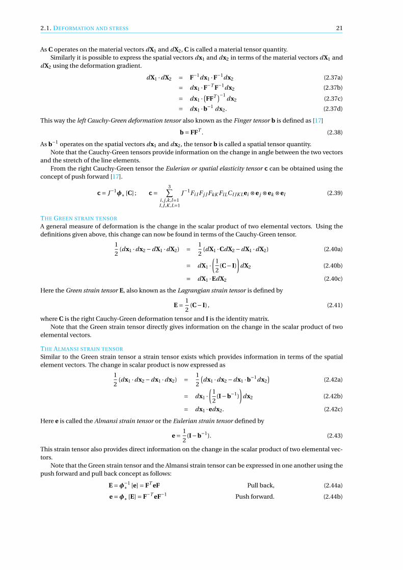
2.1. DEFORMATION AND STRESS 21
As C operates on the material vectors dX1 and dX2, C is called a material tensor quantity.Similarly it is possible to express the spatial vectors dx1 and dx2 in terms of the material vectors dX1 and
dX2 using the deformation gradient.
dX1 ·dX2 = F−1dx1 ·F−1dx2 (2.37a)
= dx1 ·F−T F−1dx2 (2.37b)
= dx1 ·(FFT )−1
dx2 (2.37c)
= dx1 ·b−1 dx2. (2.37d)
This way the left Cauchy-Green deformation tensor also known as the Finger tensor b is defined as [17]
b = FFT . (2.38)
As b−1 operates on the spatial vectors dx1 and dx2, the tensor b is called a spatial tensor quantity.Note that the Cauchy-Green tensors provide information on the change in angle between the two vectors
and the stretch of the line elements.From the right Cauchy-Green tensor the Eulerian or spatial elasticity tensor c can be obtained using the
concept of push forward [17].
c= J−1φ∗ [C] ; c=3∑
i , j ,k,l=1I ,J ,K ,L=1
J−1Fi I F j J FkK FlLC I JK Lei ⊗e j ⊗ek ⊗el (2.39)
THE GREEN STRAIN TENSOR
A general measure of deformation is the change in the scalar product of two elemental vectors. Using thedefinitions given above, this change can now be found in terms of the Cauchy-Green tensor.
1
2(dx1 ·dx2 −dX1 ·dX2) = 1
2(dX1 ·CdX2 −dX1 ·dX2) (2.40a)
= dX1 ·(
1
2(C− I)
)dX2 (2.40b)
= dX1 ·EdX2 (2.40c)
Here the Green strain tensor E, also known as the Lagrangian strain tensor is defined by
E = 1
2(C− I) , (2.41)
where C is the right Cauchy-Green deformation tensor and I is the identity matrix.Note that the Green strain tensor directly gives information on the change in the scalar product of two
elemental vectors.
THE ALMANSI STRAIN TENSOR
Similar to the Green strain tensor a strain tensor exists which provides information in terms of the spatialelement vectors. The change in scalar product is now expressed as
1
2(dx1 ·dx2 −dx1 ·dx2) = 1
2
(dx1 ·dx2 −dx1 ·b−1dx2
)(2.42a)
= dx1 ·(
1
2(I−b−1)
)dx2 (2.42b)
= dx1 ·edx2. (2.42c)
Here e is called the Almansi strain tensor or the Eulerian strain tensor defined by
e = 1
2(I−b−1). (2.43)
This strain tensor also provides direct information on the change in the scalar product of two elemental vec-tors.
Note that the Green strain tensor and the Almansi strain tensor can be expressed in one another using thepush forward and pull back concept as follows:
E =φ−1∗ [e] = FT eF Pull back, (2.44a)
e =φ∗ [E] = F−T eF−1 Push forward. (2.44b)
22 2. MATHEMATICAL MODEL
2.1.5. THE PRINCIPAL STRESSESA very common way of working with the stress of a body is to consider the principal stresses. These stressesare equal to the Cauchy stresses when the basis is changed in such a way that the shear stresses become equalto zero. This is done as follows [18].Suppose the basis that is used is given by (~e1,~e2,~e3) and the stress vector is given by ~T = σ~n. Now supposethat for this basis the stress vector on the cutting plane P (n) is not parallel to the normal ~n (see Figure 2.6).The goal is to find a cutting plane P (~n′) for which ~T =σ~n′ =λ~n′ with λ a scalar and ~n′ is parallel to ~T . Takingthis plane together with two other planes which are mutually perpendicular will form a basis of the tensor,better known as the principal basis. Note that this basis is made of the principal directions of the stress tensorwhich, due to the symmetry of σ, are the orthonormal eigenvectors of σ.
Figure 2.6: When the stress tensor is considered in a basis in which the stress in parallel to the normal one obtains the principal stresses.Source: [18]
In the principal basis the stress tensor reduces to its diagonal form and is given as
σ= σ1 0 0
0 σ2 00 0 σ3
(2.45)
Here σ1, σ2 and σ3 are the principal stresses. Note that these stresses are the roots of the characteristic equa-tion of the stress tensor σ given by
σ= σ11 σ12 σ13
σ21 σ22 σ23
σ31 σ32 σ33
. (2.46)
The roots can be calculated by solving∣∣∣∣∣∣σ11 −λ σ12 σ13
σ21 σ22 −λ σ23
σ31 σ32 σ33 −λ
∣∣∣∣∣∣= 0. (2.47)
which obtains the characteristic equation
λ3 − I1λ2 + I2λ− I3 = 0, (2.48)
where Ii are the stress invariants.
I1 =σ11 +σ22 +σ33 (2.49a)
= trσ
I2 =σ11σ22 +σ22σ33 +σ11σ33 −σ212 −σ2
23 −σ231 (2.49b)
= 1
2
[tr(σ)2 − tr(σ2)
]= 1
2
(σi iσ j j −σi jσ j i
)I3 =σ11σ22σ33 +2σ12σ23σ31 −σ2
12σ33 −σ223σ11 −σ2
31σ22 (2.49c)
= det(σ)
2.1. DEFORMATION AND STRESS 23
Note that due to the symmetry of the Cauchy stress tensor there are three real roots λi for the charac-teristic equations. These roots are the principal stresses, which are often ordered as σ1 ≥ σ2 ≥ σ3, usingequations (2.49a)–(2.49c).
σ1 = max(λ1,λ2,λ3) (2.50a)
σ2 = I1 −σ1 −σ3 (2.50b)
σ3 = min(λ1,λ2,λ3) (2.50c)
The stress invariants Ii can also be given in terms of the principal stresses:
I1 =σ1 +σ2 +σ3, (2.51a)
I2 =σ1σ2 +σ2σ3 +σ3σ1, (2.51b)
I3 =σ1σ2σ3. (2.51c)
The principal stresses and directions do not depend on the chosen axes to describe the stress as they areproperties of the stress tensor. The stress invariants I1, I2 and I3 are invariant under coordinate transforma-tion [19].
2.1.6. THE MAXIMUM SHEAR STRESSIn Section 2.1.3 the shear stress τ has been defined. A common measure when working with shear stresses isthe maximum shear stress τmax. As the stresses depend on the basis in which they are considered it is clearthat on a certain plane the stresses will be maximal.The maximum shear stress is given in terms of the principal stresses (σ1 ≥σ2 ≥σ3) as
τmax = 1
2(σ1 −σ3). (2.52)
24 2. MATHEMATICAL MODEL
2.2. PROBLEM DEFINITIONThe issue that is being considered is the problem of a bedbound patient who has a risk of the developmentof pressure ulcers. From the moment the patient lies in the bed the skin will experience a certain stress level.If the skin of the patient is exposed during a longer period of time, the stress level can increase which willweaken the skin. When a patient is then being moved across the bed by a caretaker, the skin can break down.Following the method described by Gefen and Shaked in [2], the following problem will be implemented.
• A human body is at rest on a mattress. Shaked and Gefen worked with a 2D model in which the bodywas modeled by a circle and the mattress by a rectangle. As FEBio uses 3D models the body shall nowbe modeled as a sphere and the mattress will be represented by a box.
• Due to gravity the body immerses into the mattress which will cause both the human skin and themattress to deform.
• After a while a caregiver will move the body 10cm across the mattress (horizontal sliding) and 1cmtowards the mattress. This latter movement is due to the additional loading the caregiver applies toreposition the patient.
This section contains information on the exact problem which FEBio solves, i.e. the problem describedabove written in mathematical equations. The general problem given by the equations of motion shall begiven in Section 2.2.1. This will be followed by a derivation of the weak form (Section 2.2.2) after which thefinite element method which is implemented in FEBio (Sections 3.2 and 3.4) shall be discussed. Both sectionsclosely follow the derivations given in [17], as this is the literature work on which the implementation in FEBiois based.In Section 2.3 it will be described how FEBio deals with contact problems. The information in this section isgained from [20]. Additional information on contact mechanics is given in Appendix B.
2.2.1. THE PROBLEMAs FEBio is a program in which many various problems can be implemented, different starting points areused for several types of problems. In this thesis only the case of solid materials shall be considered.
In general when looking at solid materials a good place to start mathematically is with the basic principlesfrom mechanics. These principles can be Newton’s Laws, or the equivalent set of dynamics laws Euler’s Laws.In this thesis we will start from Euler’s Laws to derive the Equations of motion, specifically Euler’s first Law:the Principle of Linear Momentum.
A distinction will be made between two types of descriptions [17].
The material description is also known as the Lagrangian description. In this description the variation of aquantity such as the material density ρ over the body is described with respect to the original (or initial)coordinate X used to label a material particle in the continuum at time t = 0 as
ρ = ρ(X, t ).
Here a change in time t means that the same material particle X has a different density ρ, hence interestis focused on the material particle X .
The spatial description is also known as the Eulerian description. In this description the quantities will bedescribed with respect to the position in the current configuration x, currently occupied by a materialparticle in the continuum at time t . For instance, the material density ρ will be described as
ρ = ρ(x, t ).
A change in time t implies that a different density is observed at the same spatial position x, now prob-ably occupied by a different particle. Interest is focused on a spatial position x.
The implementation in FEBio uses the spatial description, however, the material description is used tosimplify certain derivations.
THE PRINCIPLE OF LINEAR MOMENTUM
In the Principle of Linear Momentum the momentum of an object is defined as a measure of an objectstendency to keep moving once it is set in motion.
2.2. PROBLEM DEFINITION 25
Spatial form In the spatial form the linear momentum p is equal to the product of the body’s mass and itsvelocity.
p = mv (2.53)
When considering the change in an objects momentum over time one obtains
p = dp
d t= d(mv)
d t= m
dv
d t= ma. (2.54)
Here we used that the mass of the body is constant in time, hence dmd t = 0. Equation (2.54) can be rewritten
using Newton’s second law which states that F = ma. This gives
F = d
d t(mv) (2.55)
which is known as the principle of linear momentum, or the balance of linear momentum. Looking at theequation it states that the rate of change of the momentum is equal to the applied force. When the appliedforces are equal to zero (there are no forces applied to the system) this law is called the law of conservation of(linear) momentum. In this case the total momentum of the system remains constant.
The principles as they are given above are applied to a particle and therefore should be expanded to holdfor a continuum. We shall do this by considering a material volume v in the current configuration. Given thisfinite portion has a spatial mass density ρ(x, t ) and a spatial velocity field v(x, t ) the total linear momentumof this mass is given as
L(t ) =∫
vρ(x, t )v(x, t )d v. (2.56)
Considering the rate of change of the momentum the principle of linear momentum states that
L(t ) = d
d t
∫vρ(x, t )v(x, t )d v = F(t ), (2.57)
where F(t ) is the resultant of the forces acting on the finite portion. Note that we are working with materialvolume, which contains the same particles of matter at all times. The amount of space occupied by theseparticles may change over time.
The above equation includes a derivative of an integral, which we would like to rewrite. This can be doneby using the law of mass conservation, which states that for a density ρ and v the velocity of the element
∂ρ
∂t+∇· (ρv) = 0. (2.58)
Using this we can obtain the following for F a property per unit mass and V a material volume, where the firstequality is known as Reynolds’ transport theorem for a material element.
d
d t
(∫VρF dV
)=
∫V
∂ρF
∂tdV +
∫SρF (v ·n) dS
=∫
V
(∂ρ
∂tF +ρ ∂F
∂t+∇· (ρvF )
)dV
=∫
V
(F
[∂ρ
∂t+∇· (ρv)
]+ρ
[∂F
∂t+v ·∇F
])dV
=∫
Vρ
[∂F
∂t+v ·∇F
]dV
=∫
Vρ
DF
DtdV
Here DFDt is the material derivative of the property F , given by
DF
Dt= ∂F
∂t+v ·∇F. (2.59)
26 2. MATHEMATICAL MODEL
It can be found that the material derivative of the velocity v itself is equal to the acceleration.
Dv
Dt= ∂v
∂t+v ·∇v
= ∂v
∂t+ vx
∂v
∂x+ vy
∂v
∂y+ vz
∂v
∂
= d
d tv(t , x, y, z)
= v.
We obtain
L(t ) =∫
vρ(x, t )v(x, t )d v = F(t ). (2.60)
We can further rewrite this linear momentum principle by evaluating the resultant force F(t ) acting on thebody. This force exists of the surface tractions t acting over the surface elements and the body forces b whichact on the volume elements. Using this the resultant force can be written as
F(t ) =∫
std s +
∫v
bd v. (2.61)
Substituting this into equation (2.60) we can express
The Principle of the Linear Momentum in the spatial form as∫vρ(x, t )v(x, t )d v =
∫s
td s +∫
vbd v. (2.62)
Material form The linear momentum of a mass element in material form is given by ρ0VdV , where V is thesame velocity as v which is used in the spatial form. The only difference is that now the velocity is expressedin the material coordinates X and ρd v = ρ0dV . Similar to the spatial form, the total linear momentum can begiven as an integral over the volume V in the reference configuration:
L(t ) =∫
Vρ0(X)V(X, t ) dV. (2.63)
Using this and the law of mass conservation the principle of linear momentum is now given by
L(t ) = d
d t
∫Vρ0(X)V(X, t ) dV =
∫Vρ0
dV
d tdV = F(t ). (2.64)
The forces F are the external forces acting on the current configuration, which means that we have to workwith the first Piola-Kirchhoff stress, since this stress measures the actual force in the current configuration,however per unit surface area in the reference configuration. With this stress the surface force acting on thesurface element d s in the current configuration can be given using the first Piola-Kirchhoff traction vectorT as dfsur f = td s = TdS, where t is the Cauchy traction vector. Similarly the body force can be given by thereference body force B, which is the actual body force acting on the current configuration per unit volume inthe reference configuration. One obtains dfbod y = bd v = BdV .Using these two definitions the resultant force is
F(t ) =∫
ST dS +
∫V
B dV. (2.65)
After substituting this into equation (2.64) we obtain
The Principle of the Linear Momentum in the material form∫Vρ0
dV
d tdV =
∫S
T dS +∫
VB dV. (2.66)
2.2. PROBLEM DEFINITION 27
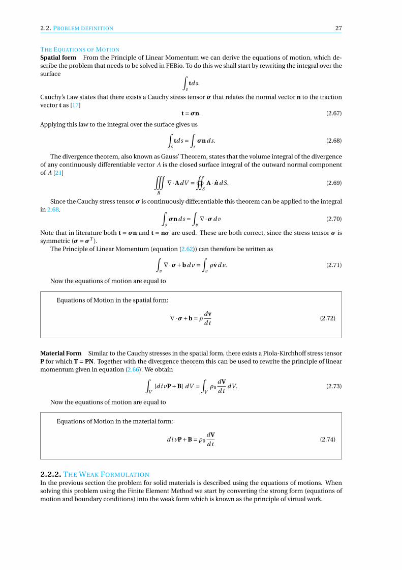
THE EQUATIONS OF MOTION
Spatial form From the Principle of Linear Momentum we can derive the equations of motion, which de-scribe the problem that needs to be solved in FEBio. To do this we shall start by rewriting the integral over thesurface ∫
std s.
Cauchy’s Law states that there exists a Cauchy stress tensor σ that relates the normal vector n to the tractionvector t as [17]
t =σn. (2.67)
Applying this law to the integral over the surface gives us∫s
td s =∫
sσn d s. (2.68)
The divergence theorem, also known as Gauss’ Theorem, states that the volume integral of the divergenceof any continuously differentiable vector A is the closed surface integral of the outward normal componentof A [21] Ñ
R
∇·A dV =Ó
SA · n dS. (2.69)
Since the Cauchy stress tensorσ is continuously differentiable this theorem can be applied to the integralin 2.68. ∫
sσn d s =
∫v∇·σd v (2.70)
Note that in literature both t = σn and t = nσ are used. These are both correct, since the stress tensor σ issymmetric (σ=σT ).
The Principle of Linear Momentum (equation (2.62)) can therefore be written as∫v∇·σ+b d v =
∫vρv d v. (2.71)
Now the equations of motion are equal to
Equations of Motion in the spatial form:
∇·σ+b = ρdv
d t(2.72)
Material Form Similar to the Cauchy stresses in the spatial form, there exists a Piola-Kirchhoff stress tensorP for which T = PN. Together with the divergence theorem this can be used to rewrite the principle of linearmomentum given in equation (2.66). We obtain∫
V[di vP+B] dV =
∫Vρ0
dV
d tdV. (2.73)
Now the equations of motion are equal to
Equations of Motion in the material form:
di vP+B = ρ0dV
d t(2.74)
2.2.2. THE WEAK FORMULATIONIn the previous section the problem for solid materials is described using the equations of motions. Whensolving this problem using the Finite Element Method we start by converting the strong form (equations ofmotion and boundary conditions) into the weak form which is known as the principle of virtual work.
28 2. MATHEMATICAL MODEL
SPATIAL FORM
Starting with the equations of motion in the spatial form (equation (2.72)) the weak form is derived by multi-plying the equation by a test function δv which represents a virtual velocity and integrate over the volume v .By doing so we obtain ∫
vδv(∇·σ+b) dV =
∫vδv(ρ
dv
d t) dV. (2.75)
The above equation can be rewritten using the fact that (σ=σT ) and the identity
∇(AT ·b) = b · (∇· A)+ A : (∇b),
or, in a different order,b · (∇· A) =∇(AT ·b)− A : (∇b).
We obtain ∫vδv(∇·σ) d v =
∫v∇· (σ ·δv) d v −
∫vσ : (∇δv) d v, (2.76)
from which follows that ∫vδv(ρ
dv
d t) d v =
∫v
[∇· (σ ·δv)−σ : (∇δv)+δv ·b] d v. (2.77)
Here the divergence theorem (equation (2.69)) can be applied followed by Cauchy’s law (equation (2.67)).∫vδv(ρ
dv
d t) d v =
∫∂v
[(σ ·δv) ·n] d a −∫
vσ : (∇δv) d v +
∫v
[δv ·b] d v
=∫∂v
(t ·δv) d a −∫
vσ : (∇δv) d v +
∫v
[δv ·b] d v, (2.78)
where we used that(σ ·δv) ·n ≡σi j∂v j ni = ∂v jσ j i ni ≡ δv · (σ ·n) = δv · t = t ·δv.
Changing the order of these integrals we obtain:
−∫
vδv(ρ
dv
d t) d v =
∫vσ : (∇δv) d v −
∫v
[b ·δv] d v −∫∂v
(t ·δv) d a. (2.79)
FEBio allows the user to choose between quasi-static and a dynamic analysis, where the quasi-static anal-ysis is the default setting. In the quasi-static analysis the inertial effects, given by the ρ-term, are ignored andan equilibrium solution is sought. This means that they work with the equations of equilibrium in which theacceleration dv
d t is taken equal to zero and hence∫vσ : (∇δv) d v −
∫v
[b ·δv] d v −∫∂v
(t ·δv) d a = 0. (2.80)
Note that this equation includes the expression ∇δv. As δv is an arbitrary virtual velocity, the gradient ofthis velocity is by definition the virtual velocity gradient δl, defined as
δl =∇δv = ∂δv
∂x=
∂δvx∂x
∂δvx∂y
∂δvx∂z
∂δvy
∂x∂δvy
∂y∂δvy
∂z∂δvz∂x
∂δvz∂y
∂δvz∂z
. (2.81)
Using this, equation (2.80) becomes∫vσ : δl d v −
∫v
[b ·δv] d v −∫∂v
(t ·δv) d a = 0. (2.82)
As a final step the virtual velocity gradient is expressed in terms of the symmetric virtual rate of deforma-tion δd and the antisymmetric virtual spin tensor δw as
δl = δd+δw, (2.83)
2.2. PROBLEM DEFINITION 29
where
δd = 1
2(δl+δlT ),and (2.84a)
δw = 1
2(δl−δlT ). (2.84b)
Assuming the rotational motion of the particles is equal to zero, the spatial virtual work equation can beformulated using spatial quantities only.
The spatial virtual work equation:
δW =∫
vσ : δd d v −
∫v
b ·δv d v −∫∂v
t ·δv d a = 0. (2.85)
MATERIAL FORM
The virtual work equation in material form can be derived in two different ways. First of all, it can be deriveddirectly from the equations of motion. Secondly it is possible to derive the material form from the spatialform. In this section the entire virtual work equation shall be derived from the equations of motion, afterwhich only a part of the virtual work equation shall be derived from the spatial form. Even though the resultsare the same the latter way is used later on in the Newton Raphson Method and is therefore shown here.
Derivation from the equations of motion Starting with the equations of motion in material form (equation(2.74)) the derivation of the Principle of Virtual Work in material form is quite similar to the derivation of thespatial form.
di vP+B = ρ0dV
d t(2.86)
The first step is to multiply both sides by a test function δV and to take the integral over the volume V .∫VδV (di vP+B) dV =
∫VδV
(ρ0
dV
d t
)dV. (2.87)
Note that unlike the Cauchy stress tensor σ, the PK1 stress tensor P is not symmetric. Using
b · (∇· A) =∇(AT ·b)− A : (∇b),
one therefore obtains ∫VδV (∇·P) dV =
∫V∇· (PT ·δV
)dV −
∫V
P : (∇δV) d v. (2.88)
Substituting this into equation (2.87) gives∫VδV(ρ0
dV
d t) dV =
∫V
[∇· (PT ·δV)−P : (∇δV)+δV ·B]
dV. (2.89)
Here the divergence theorem (equation (2.69)) can be applied after which one can use that PN = T.∫VδV(ρ0
dV
d t) dV =
∫∂V
[PT ·δV) ·N
]d A−
∫V
P : (∇δV) dV +∫
V[δV ·B] dV
=∫∂V
[δV ·P) ·N] d A−∫
VP : (∇δV) dV +
∫V
[δV ·B] dV
=∫∂V
[T ·δV] d A−∫
VP : (∇δV) dV +
∫V
[δV ·B] dV (2.90)
Changing the order of these integrals, gives
−∫
VδV(ρ0
dV
d t) dV =
∫V
P : (∇δV) dV −∫
V[B ·δV] dV −
∫∂V
(T ·δV) d A. (2.91)
Similar to the spatial case the acceleration dVd t is taken equal to zero because the inertial effects are ignored
and an equilibrium solution is sought, which gives
30 2. MATHEMATICAL MODEL
The material virtual work equation:
δW =∫
VP : (∇δV) dV −
∫V
[B ·δV] dV −∫∂V
(T ·δV) d A = 0. (2.92)
Derivation from the spatial form The second way of determining the material form of the virtual workequation is through the spatial form. Here only a part of the equation shall be derived, as this is the only partthat is needed. We start with the following expression in the spatial form [17]:∫
vσ : δd d v. (2.93)
In this derivation the virtual work shall be expressed using the second Piola-Kirchhoff stress tensor S and thetime derivative of the Green strain tensor E.
First of all the time derivative of the Langangian strain tensor will be considered. This tensor E is knownas the material strain rate tensor [17]. Here E = 1
2 (C− I) is the Lagrangian strain tensor. The derivative is nowobtained by
E = 1
2C = 1
2
(FT F+FT F
). (2.94)
Here C = FT F is the right Cauchy-Green deformation tensor as defined in equation (2.36).
The material strain rate tensor gives the current rate of change of the scalar product of two elementalvectors in terms of the initial elemental vectors as
d
d t(dx1 ·dx2) = 2dX1 · EdX2. (2.95)
The rate of change of the scalar product can also be expressed in terms of dx1 and dx2 as
1
2
d
d t(dx1 ·dx2) = dX1 · EdX2
= F−1dx1 · EF−1dx2
= dx1 ·(F−T EF−1)dx2. (2.96)
In this equation the rate of deformation tensor d is introduced which is defined as
d = F−T EF−1. (2.97)
Another way of defining the rate of deformation tensor is by using the velocity gradient l. This gradient isdefined as
l = ∂v(x, t )
∂x=∇v, (2.98)
where v(x, t ) is the velocity as a function of the spatial coordinates. Another way of defining l is by
l = FF−1. (2.99)
With these definitions of the velocity gradient the rate of deformation tensor can be given by
d = 1
2(l+ lT ). (2.100)
Note that the material strain rate tensor and the rate of deformation tensor can be expressed in one an-other using the push forward and pull back concept as follows:
E =Ψ−1∗ [d] = FT dF Pull back, (2.101a)
d =Ψ∗[E]= F−T EF−1 Push forward. (2.101b)
2.2. PROBLEM DEFINITION 31
Using these new definitions, the virtual work equation can be rewritten into the material form [17].∫vσ : δd d v =
∫V
Jσ :(F−TδEF−1) dV (2.102a)
=∫
Vtr
(F−1 JσF−TδE
)dV (2.102b)
=∫
VS : δE dV (2.102c)
Note that this part is equal to the part∫
V P : (∇δV) dV in equation (2.92).
32 2. MATHEMATICAL MODEL
2.3. INCLUDING THE CONTACT DEFINITIONSOne of the most difficult parts of solving the model is the contact between the skin and the mattress. Asfurther explained in Appendix B, the biggest problem is the number of unknowns. As one cannot predict themovement and deformation of both bodies, the contact area between the bodies is also unknown.FEBio includes many options regarding contact and coupling. These different options are further explained inSection 2.4.1. In this model the contact is between two deformable bodies which will also be the contact typethat will be described in this section. This section will start with a definition of the two body contact problem(Section 2.3.1), after which it will be included in the equations of motion (Section 2.3.3). As the contact willalso be solved using the Newton-Raphson method the equations of motion including the contribution of thecontact tractions will be converted to the virtual work equation (Section 2.3.4).The definitions and derivations in this section closely follow the information given in [20], as this is the bookthat was used for the implementation in FEBio.
2.3.1. THE TWO BODY CONTACT PROBLEMBefore discussing the problem some notation shall be introduced [20]. The two bodies that are consideredin the reference configuration are denoted by Ω(i ) ⊂ R3 for i = 1,2. The bodies are put in motion, describedby ϕ(i ) which will cause them to come into contact. Points within the first body Ω(1) are denoted by X in thereference configuration and x in the current configuration. Points in the second body Ω(2) are denoted byY and y respectively. The boundary of each body in the reference configuration is denoted as ∂Ω(i ) and issubdivided into three regions Γ(i )
c , Γ(i )σ and Γ(i )
u , such that
Γ(i )c ∪Γ(i )
σ ∪Γ(i )u = ∂Ω(i ), and Γ(i )
c ∩Γ(i )σ = Γ(i )
c ∪Γ(i )u = Γ(i )
u ∪Γ(i )σ =;. (2.103)
The three regions are defined as follows:
• Γ(i )c is the part of the boundary that is in contact with the other body,
• Γ(i )σ is the part of the boundary where tractions are applied, and
• Γ(i )u is the part of the boundary where the solution (the displacement u(i )) is prescribed.
Figure 2.7: The basic notation used in the two body contact problem. Source: [20].
In the current configuration the counterpart of the contact boundary is designated as γ(i )c = ϕ(i )
t
(Γ(i )
c
),
i = 1,2. An overview of the notation is given in Figure 2.7.Recall from Section 2.2.1 that the equations of motion in the material form are given by equation (2.74)
where P is the first Piola-Kirchhoff stress, B the prescribed body force, ρ0 the reference density and dVd t the
material acceleration field:
di vP+B = ρ0dV
d t. (2.104)
As this equation must hold for each body separately, the equation can be written for body i as
di vP(i ) +B(i ) = ρ(i )0 A(i ), where A(i ) = dV(i )
d t. (2.105)
2.3. INCLUDING THE CONTACT DEFINITIONS 33
Similarly in the spatial form:
∇·σ(i ) +b(i ) = ρ(i )a(i ), where a(i ) = dv(i )
d t. (2.106)
The corresponding initial and boundary conditions are given by
P(i )N(i ) = T(i ) in Γ(i )σ , for all t , (2.107a)
ϕ(i ) = ϕ(i ) in Γ(i )u , for all t , (2.107b)
ϕ(i )∣∣∣
t=0= V(i )
0 in Ω(i ), (2.107c)
ϕ(i )∣∣∣
t=0= I (the identity mapping) in Ω(i ). (2.107d)
Here N(i ) is the outward normal to ∂Ω(i ) in the reference configuration, T(i ) is the specified traction field onΓ(i )σ , ϕ(i ) is the specified displacement field on Γ(i )
u and V(i )0 is the specified initial velocity field for body i .
The final element that needs to be introduced before introducing the contact element in the equation ofmotion are the contact conditions describing the response on Γ(1)
c (or Γ(2)c ). The first step in introducing these
conditions is terming the two bodies.
1. The first body has the surface that will be used to parametrize the contact. The positions of pointsbelonging to this surface will be monitored with respect to the location of the second surface. Thissurface is termed the slave or contactor surface.
2. The surface of the second body is termed the master or target surface.
In this section the first body shall be parametrized, that is Γ(1)c is the slave surface, and Γ(2)
c is the mastersurface.
Now for a given point X on the slave reference contact surface Γ(1)c , there is a point Y(X) on the master
contact surface (Γ(2)c ) that is ’closest’ to point X. This point Y(X) is defined according to the following closest
point projection:
Y(X) = arg minY∈Γ(2)
c
∥∥∥ϕ(1)t (X)−ϕ(2)
t (Y)∥∥∥ . (2.108)
With this definition of the closest point, the gap function g (X, t ) can be written as
g (X, t ) =−v(ϕ(1)
t (X)−ϕ(2)t (Y(X))
), (2.109)
where v is the outward unit normal to γ(2)ct
at y =ϕ(2)t (Y). Note that when g > 0 it means that X has penetrated
body 2, which is not allowed when dealing with contact. From this the contact constraint condition can bederived as being
g (X, t ) ≤ 0. (2.110)
2.3.2. INCLUDING FRICTION IN THE PROBLEMNow that the contact problem has been described, the effects of friction can be included. Since the contactis described from the position of points X ∈ Γ(1)
c opposing the surface Γ(2)c , the goal is to write the frictional
governing equations in a similar way. For this some new notation needs to be introduced. The notation startswith assuming that Γ(2)
c can be described as
Γ(2)c =Ψ(2)
0 (A (2)), and γ(2)c =Ψ(2)
t (A (2)), (2.111)
where A (2) ⊂R2 is a parametrization of the contact surface, see Figure 2.8.This parametrization A (2) and the mappingsΨ(2)
0 andΨ(2)t are assumed to be smooth for simplicity [20].
Typical points of A (2) will be denoted by ξ. The point of A (2) corresponding to Y(X, t ) will be denoted byξ(X, t ).It is convenient to define bases associated with each point X, which are advected with X as it moves. Thesebases shall be called the slip advected bases. The first one that will be defined is one in the reference configu-ration of the sliding surface (Γ(2)
c ). The second is defined in the current configuration (γ(2)c ).
Tα :=Ψ(2)0,α(ξ(X, t )), and τα :=Ψ(2)
t ,α(ξ(X, t )), α= 1, . . .nsd −1. (2.112)
34 2. MATHEMATICAL MODEL
Figure 2.8: Schematic of the parametrization of a contact surface. Source: [20].
Here nsd is the number of spatial dimensions. Note that Tα and τα are always associated with a materialpoint X and are evaluated according to its current (closest point) projection to Γ(2)
c , parametrized by ξ(X, t ).When characterizing potential frictional response the most important variable is the relative velocity betweenX and its opposing point Y(X, t ). This relative velocity can be expressed both in the spatial configuration andthe reference configuration, by an appeal to the slip advected bases introduced in equation (2.112). We con-sider the time derivative of the relative position vector between x =ϕ(1)(X) and its contact point y =ϕ(2)(Y(X))during perfect sliding (when g = g = 0) and the two points remain coincident in space [20].
0 = d
d t
[ϕ(1)(X, t )−ϕ(2)(Y(X, t ), t )
]= V(1)(X, t )−V(2)(Y(X, t ), t )−F(2)
t (Ψ(2)0 (ξ(X, t )))
d
d t[Y(X, t )] (2.113)
Here F(2)t is the deformation gradient of body (2) at time t . From this equation it follows that the relative
velocity may be represented in terms of vectors in the tangent spaces Γ(2)c and γ(2)
c while sliding is occurring.The spatial relative velocity υT and the convective relative velocity νT are defined as
υT := F(2)t
(Ψ(2)
0 (ξ(X, t ))) d
d t[Y(X, t )], (2.114a)
= V(1)(X, t )−V(2)(Y(X, t ), t ) by equation (2.113), and
νT := d
d t[Y(X, t )], (2.114b)
= ˙ξα(X, t )Tα as the point in A (2) corresponding toY(X, t ) is denoted by ξ(X, t ).
It can be shown that νT is the pull back of υT byϕ(2)t and since
τα = F(2)t Tα, (2.115)
it follows thatυT = ˙ξα(X, t )τα. (2.116)
It can be derived ([20]) that the ˙ξα are the components of the convected relative velocity V T with respectto the Tα basis, and are likewise the components of the spatial relative velocity υT with respect to theτα basis.
More generally, the components ˙ξα(X, t ) of υT and νT in their respective basis can be interpreted usingthe closest point projection given in equation (2.108). This can even be done for the case where g 6= 0. It canbe noted that since the projection of x =ϕ(1)
t (X) onto γ(2)ct
is normal to γ(2)ct
at y =ϕ(2)t (Y(X)), we can write [20]
τα ·[ϕ(1)
t (X, t )−ϕ(2)t (Y(X, t ), t )
]= 0, α= 1,2. (2.117)
Taking the material time derivative of this expression yields
0 =[
V(1)(X)−V(2)(Y(X))−τγ ˙ξγ]·τα− gν ·
[V(2)
,α (Y(X))+ϕ(2)t ,αβ(ξ)˙ξβ
]. (2.118)
2.3. INCLUDING THE CONTACT DEFINITIONS 35
This can be rewritten as
Aαβ˙ξβ = [
V(1)(X)−V(2)(Y(X))]τα− gν · [V(2)
,α (Y(X))]
, (2.119)
where the quantity Aαβ is defined as
Aαβ := mαβ+ gκαβ. (2.120)
In this equation καβ := ν ·ϕ(2)t ,αβ(Y) denotes the components of the surface curvature at ξ [20], and mαβ :=
τα ·τβ refers to the components of the metric tensor.
In the case of perfect sliding, i.e. when g = 0, equation (2.119) simplifies to
˙ξα = [V(1)(X)−V(2)(Y(X))
]τα. (2.121)
Here τα = mαβτβ represents the dual basis to τβ.
It can be obtained that in the case of perfect sliding the ˙ξα represent the projection of the relative materialvelocity V(1)(X)−V(2)(Y(X)) into the (spatial) tangent plane atϕ(2)
t (Y(X)).
To formulate the frictional model a distinction shall be made between two frameworks: the spatial kine-matic frame and the convected kinematic frame.
Starting with the spatial kinematic frame, the spatial relative velocity υT will be used in the equations.Note that even though the quantity is associated with the material point X, it is a vector resolved in terms ofspatial bases τα. Considering the Piola-Kirchhoff contact traction T(X, t ), one finds that this vector can alsobe written in terms of spatial bases. Recall that the Piola traction is defined as
T(X, t ) := P(X, t )N(X), (2.122)
where P is the first Piola-Kirchhoff stress and N the outward surface normal in the initial configuration.A frictional traction vector can be defined by resolving the Piola traction T(X, t ) in terms of the spatial basis toobtain the (spatial) frictional traction tT :
tT (X, t ) :=−T(X, t )+ tN (X, t )ν, (2.123)
where tN is the contact pressure, which is positive if it is compressive, and ν is the outward normal to γ(2)c at
ϕ(2)t (Y(X, t )). The minus sign ensures that tT physically represents the frictional traction exerted by X on the
surface Γ(2)c .
Considering the convected kinematic frame allows for the frictional traction to be defined in the con-vected basis. The convected frictional traction T T (X, t ) is defined as the pull back of tT induced byϕ(2)
t :
T T (X, t ) := F(2)T
t (Y(X, t ))tT (X, t )
= tTα (X, t )Tα. (2.124)
In this equation the last line holds due to the fact that Tα = F(2)T
t τα.
COULOMB FRICTION
With the two frameworks defined above we can now turn to friction. FEBio supports contact with Coulombfriction, which is the most common form of friction (see Appendix B.2.4). The friction will be formulatedwithin both frameworks. The Coulomb law for large sliding problems shall be given in the unregularizedform, which is not differentiable at the origin and allows for description of perfect sticking behavior [20].The Coulomb law states that the frictional traction force tT should always be smaller than or equal to thecontact pressure tN multiplied by a coefficient of friction µ:
‖tT ‖ ≤µtN . (2.125)
36 2. MATHEMATICAL MODEL
In the spatial slip advected frame the Coulomb law can be expressed as
g ≤ 0
tN ≥ 0
tN g = 0
Ψ(tT ,tN ) := ‖tT ‖−µtN ≤ 0, (2.126)
υbT = γ
tT
‖tT ‖,
γ ≥ 0,
γΨ = 0.
Here υbT = mαβ
˙ξβτα, with mαβ = τα ·τβ as before, and ‖(•)‖ indicating the Euclidean norm of the vector (•).The indicesα,β,γ, . . . run between 1 and nsd −1. Equation (2.126) can be written in components (with respectto the τα basis) as
g ≤ 0
tN ≥ 0
tN g = 0
Ψ(tT ,tN ) := [tTαmαβtTβ ]1/2 −µtN ≤ 0, (2.127)
mαβ˙ξβτα = γ
tTα
[tTβmβγtTγ ]1/2,
γ ≥ 0,
γΨ = 0.
In the convective slip advected frame the Coulomb law can be written as
g ≤ 0
tN ≥ 0
tN g = 0
Ψ(T T ,tN ) := ‖T T ‖−µtN ≤ 0, (2.128)
V bT = γ
T T
‖T T ‖,
γ ≥ 0,
γΨ = 0.
With respect to the Tα basis this can be written in components as
g ≤ 0
tN ≥ 0
tN g = 0
Ψ(tT ,tN ) := [tTαMαβtTβ ]1/2 −µtN ≤ 0, (2.129)
Mαβ˙ξβτα = γ
tTα
[tTβMβγtTγ ]1/2,
γ ≥ 0,
γΨ = 0.
Here Mαβ = Tα ·Tβ is the material metric. Note that though the expressions given in (2.127) and (2.129)
are very similar, they are not entirely identical. Where the spatial description uses spatial metrics mαβ tocompute lengths, the convective frame uses reference metrics Mαβ for this. This results in a spatial tractiontT in the spatial frame which satisfies Coulombs law, while in the convective frame T T is forced to satisfy thislaw. When the deformation of Γ(2)
c is small however, these differences vanish.
2.3. INCLUDING THE CONTACT DEFINITIONS 37
2.3.3. INCLUDING THE CONTACT IN THE EQUATIONS OF MOTIONWith the definitions given in the previous section, the total problem including the contact constraints is givenby [20]:
di vP(i ) +B(i ) = ρ(i )0 A(i ), where A(i ) = dV(i )
d t. (2.130)
The corresponding initial boundary conditions are given by
P(i )N(i ) = T(i ) in Γ(i )σ , for all t (2.131a)
ϕ(i ) = ϕ(i ) in Γ(i )u , for all t (2.131b)
ϕ(i )∣∣∣
t=0= V(i )
0 in Ω(i ) (2.131c)
ϕ(i )∣∣∣
t=0= I (the identity mapping) in Ω(i ) (2.131d)
Note that thus far the problem is stated the same as the problem without contact. Now the additional infor-mation that needs to be incorporated into the problem are the contact conditions. For all X ∈ Γ(1)
c , decom-posing the Piola-Kirchhoff traction at X as T =−tTατ
α+ tNν), the contact conditions are
tN ≥ 0 (2.132a)
g ≤ 0 (2.132b)
tN g = 0, (2.132c)
where the frictional tractions are given in either the spatial slip advected frame or the convective slip advectedframe:
• The spatial, slip advected frame:
Ψ(tT ,tN ) := [tTαmαβtTβ ]1/2 −µtN ≤ 0,
mαβ˙ξβτα = γ
tTα
[tTβmβγtTγ ]1/2,
γ ≥ 0,
γΨ = 0.
• The convective, slip advected frame:
Ψ(tT ,tN ) := [tTαMαβtTβ ]1/2 −µtN ≤ 0,
Mαβ˙ξβτα = γ
tTα
[tTβMβγtTγ ]1/2,
γ ≥ 0,
γΨ = 0.
2.3.4. THE WEAK FORM INCLUDING THE CONTACT TRACTIONSIn Section 2.2.2 the virtual work equation in material form is given as
δW (Ψ,δv) =∫
VP : (∇δv) dV −
∫V
[B ·δv] dV −∫∂V
(T ·δv) d A = 0. (2.133)
Here P is the PK1 stress, B the body force and T the surface traction.In the two body contact problem including friction this weak form shall only change slightly.
First of all, the above equation must hold for each body (i ), i = 1,2. Secondly, the equation will be in terms ofthe motion of body (i )ϕ(i ) and a weighting (test) functionω(i ), where
ϕ : Ω(1) ∪ Ω(2) →R3,ω : Ω(1) ∪ Ω(2) →R3.
(2.134)
Thirdly, the integral over the surface (∂V ) describing the surface tractions can be written as the integral overthe part of the surface where tractions are present (Γ(i )
σ ). Last of all, an additional term appears in the virtual
38 2. MATHEMATICAL MODEL
work equation, describing the contact problem. This term will be an integral over the part of the surfacewhere the body is in contact with the other body (Γ(i )
c ). With these changes, the virtual work equation foreach body can be written as
δW (i )(ϕ(i ),ω(i )) =∫Ω(i )
∇ω(i ) : P(i ) dΩ−∫Ω(i )
ω(i ) ·B(i ) dΩ−∫Γ(i )σ
ω(i ) ·T(i ) dΓ−∫Γ(i )
c
ω(i ) ·T(i ) dΓ= 0. (2.135)
As this equation must hold for each body the total virtual work equation for the two body contact problemcan be expressed as the summation over the bodies.
δW (ϕ,ω) :=2∑
i=1δW (i )(ϕ(i ),ω(i ))
=2∑
i=1
∫Ω(i )
∇ω(i ) : P(i ) dΩ−∫Ω(i )
ω(i ) ·B(i ) dΩ−∫Γ(i )σ
ω(i ) ·T(i ) dΓ
︸ ︷︷ ︸
δW i nt ,ext (ϕ,ω)
−2∑
i=1
∫Γ(i )
c
ω(i ) ·T(i ) dΓ︸ ︷︷ ︸δW c (ϕ,ω)
= 0. (2.136)
Note that δW i nt ,ext (ϕ,ω) denotes the internal and external virtual work that has been discussed before.δW c (ϕ,ω) denotes the contact virtual work, and is also known as the contact integral. In short equation(2.136) can be written as
δW (ϕ,ω) = δW i nt ,ext (ϕ,ω)+δW c (ϕ,ω) = 0. (2.137)
Note that the contact integral includes two integrals, one over each contact surface. This expression canbe converted to an expression including only one integral using the assumption made earlier that all contactquantities are parametrized by X ∈ Γ(1)
c . The conversion can be achieved by enforcing linear momentumacross the contact interface [20]. This is done by requiring that the differential contact force induced on body(2) at Y be equal and opposite to that produced on body (1) at X, that is
t(2)t (Y(X))dΓ(2)
c = t(1)t (X)dΓ(1)
c . (2.138)
Using this the contact integral can be given as
δW c (ϕ,ω) =−∫Γ(1)
c
t(1)t (X)
[ω(1)(X)−ω(2)(Y(X))
]dΓ. (2.139)
This can be simplified using the linearized variation of the gap function δg and the linearized variation of ξ.
δW c (ϕ,ω) =−∫Γ(1)
c
[tNν− tTατα] · [ω(1)(X)−ω(2)(Y(X))
]dΓ
δW c (ϕ,ω) =∫Γ(1)
c
[tNtδg + tTαtδξ
α]
dΓ, (2.140)
where
δg =−ν · [ω(1)(X)−ω(2)(Y(X))]
, and (2.141)
δξα =τα · [ω(1)(X)−ω(2)(Y(X))
](when g = 0). (2.142)
2.4. CONSTRUCTING THE MODEL USING THE GIBBON TOOLBOX AND FEBIO 39
2.4. CONSTRUCTING THE MODEL USING THE GIBBON TOOLBOX AND FEBIO
2.4.1. THE BASIC MODELIn this section an overview of the different components of the model is given. This will be done in a setupsimilar to the general FEBio file.
THE UNITS
FEBio allows the user to choose its own set of units. It is up to the user to verify if the set is indeed consistent.Before discussing the entire model an overview will therefore be given of used units.
Table 2.1: The used units.
Units
Time seconds s
Length millimeter mm
Mass kilogram kg
Density mass per unit volume kg/mm3
Force millinewton kg·mm/s2, mN
Stress Kilo Pascal mN/mm2, kPa
GENERAL INFORMATION
Before defining the actual problem, some general information has to provided in the .feb file. Details like thetype of problem and the name of the problem have to be given here.
FEBio allows the user to choose from five different problem modules, which define the type of analysisthat FEBio performs. The module types will be briefly discussed below [22].
Solid The solid type deals with structural mechanics problems. The user has the choice between a quasi-static analysis and a dynamic analysis.
Biphasic The biphasic module type allows the user to solve problems in which fluids flow. One can chooseto use a steady-state analysis or a transient analysis.
Solute This type is very similar to the biphasic analysis but also includes problems that include solute trans-port. Similar to the biphasic problem the user can choose between a steady-state analysis or a transientanalysis.
Multiphasic Even more elaborate is the multiphasic type in which the user can analyse problems includingchemical reactions.
Heat The heat type can be used to solve heat transfer problems. Again one has the option to choose for asteady-state analysis or a transient analysis.
In the descriptions above one can see that besides the modules the user can also choose between someanalysis types. In the solid type, which is the module that is used in this project, one can choose between aquasi-static analysis and a dynamic analysis. The difference between these two analysis types is that in thequasi-static analysis the inertial effects are ignored and an equilibrium solution is sought. In a dynamic anal-ysis the inertial effects are included. Note that even though the quasi-static analysis looks for an equilibriumsolution, it is still possible to simulate time dependent effects.In this project the Solid module with a quasi-static analysis has been used.
Besides the analysis type the user also needs to specify some control information such as the initial stepsize d t for the Newton method and total number of time steps. As the method does not always converge forlarge step sizes the user needs to specify the minimum step size that the program can use and the number ofretries that it is allowed to use. As the problem is solved using BFGS (see Section 3.4.1) the user can specify themaximum number of stiffness updates. Many of these control parameters have a default value which meansthat the user is not obliged to define them. When not defined the program will automatically use the defaultvalues. Which values do need to be given can be found in the user manual of FEBio [22].
40 2. MATHEMATICAL MODEL
GEOMETRY AND MESH
When starting to build the model using the Gibbon Toolbox and FEBio the first thing that was noted was thatthis model would have to be in 3D instead of 2D. In this model the body is therefore modeled by a sphereinstead of a circle and the bed is modeled as a box. To represent the different skin layers (i.e. skin and sub-cutaneous tissue) multiple spheres were modeled within each other. The mattress and the human body areimplemented separately, positioned to make sure they only touch each other in a single point.
The dimensions of the model During the project two different sized models have been used. Details re-garding these two models are given in Table 2.2. In working with the models the sizes of the spheres weresometimes altered to see the effect on the stress levels. Table 2.2 however gives the general dimensions.
Table 2.2: Dimensions of the two basic models.
Model A (small) Model B (big)
Width mattress 12 mm 400 mm
Thickness mattress 12 mm 400 mm
Height mattress 6 mm 50 mm
Inner radius subcutaneous tissue 2 mm 163 mm
Outer radius subcutaneous tissue 4 mm 178 mm
Inner radius skin 4 mm 178 mm
Outer radius skin 6 mm 180 mm
To give a better idea regarding the geometry of the model, both models A and B are shown in Figure 2.9.One can see that both models are currently hollow and the body only exists of skin and subcutaneous tissue.
(a) The geometry of model A (b) Cut-view of model A (c) The geometry of model B (d) Cut-view of model B
Figure 2.9: The geometry and cut-view overviews of the basic models.
Meshing the geometry Working in Matlab there are multiple ways of implementing the geometry and mesh.The first option is to model a sphere and a box and then use some software to mesh the volumes. This soft-ware could for instance be TetGen ([23]). Another option is to immediately mesh the bodies while creatingthem. In implementing the model the latter option was used. This was done using a function from the Gib-bon Toolbox in Matlab [14]. Multiple functions are available, depending on the type of elements the userwants. In this model we use 8-node hexahedral elements (hex8).While creating the mattress, the box is immediately subdivided into elements. When defining the size of thebox the user also has to define the number of elements that should fill each dimension. This can be donein different ways. The first possibility is simply stating the number of elements that have to be in the width,thickness and height. Another possibility is stating the size of the elements and defining the number of ele-ments by checking how many elements of that size can fit in the box. Of course when doing so the number ofelements need to be rounded. In the code below the latter option is shown.
2.4. CONSTRUCTING THE MODEL USING THE GIBBON TOOLBOX AND FEBIO 41
1 %% Creating the box ( mattress )sampleWidth=400; %width of the mattresssampleThickness =400; %thickness of the mattresssampleHeight =50; %height of the mattresspointSpacing =40.3;% s i z e of the elements
6
%the number of elements in the width of the boxnumElementsWidth=round ( sampleWidth/ pointSpacing ) ;%the number of elements in the thickness of the boxnumElementsThickness=round ( sampleThickness/ pointSpacing ) ;
11 %the number of elements in the height of the boxnumElementsHeight=round ( sampleHeight/ pointSpacing ) ;
Meshing the spheres is done rather similarly. The user starts with defining the inner and outer radius ofthe first sphere. This is the inner sphere, which represents the subcutaneous tissue. Immediately the user candefine whether or not the sphere should be hollow or not. If it is hollow the sphere with the inner radius willbe left empty. If not, the inner sphere and the mantel around the sphere will be united into one sphere. Whendefining the dimensions of the inner sphere the user also has to specify the number of elements that shouldbe in the core, and the number of elements that should be in the mantel. These numbers are then used toconstruct the actual sphere. Given the number of elements that the user has specified to be in the core, acube is constructed in which each dimension exists of the specified number of elements. This cube is thenchanged into a sphere. Note that the number of elements specified to be in the core is not the actual numberof elements in the core.Once the core is constructed the mantel is constructed upon this sphere. The user has specified the numberof elements that the mantel should contain and the thickness of the mantel. On every element of the outerface of the core a new element is build, of which the thickness is equal to the thickness of the mantel dividedby the number of elements in the mantel. Again the number that is specified is not equal to the actual numberof elements in the mantel.
%% Creating the f i r s t sphere ( Subcutaneous t i s s u e )sphereRadius =178; %What i s the outer radius of the f i r s t sphere
3 sphereRadiusInner =163; %What i s the inner radius of the f i r s t sphere
% How many elements should each dimension of the cube contain ?cPar . numElementsCore=10;% In how many elements should the thickness of the mantel be divided ?
8 cPar . numElementsMantel=3;% 1 means the sphere i s hollow ; 0 means the core w i l l be f i l l e d .cPar . Totaq =1;%Creating sphere[ meshStruct ]=hexMeshSphere ( cPar ) ;
When this is done only the first sphere has been constructed (the subcutaneous tissue). For the second sphere(the skin), another mantel will be constructed around the subcutaneous tissue. Here again the user needs tospecify the thickness of the mantel and the number of elements in the mantel, after which the mantel isconstructed in the same way as described above.
42 2. MATHEMATICAL MODEL
BOUNDARY CONDITIONS AND LOADS
In the model there are two different types of boundary conditions that can be used. The first one is the fixedboundary condition, in which the movement of the boundary is set to zero in a certain direction. The secondtype is the prescribed boundary condition. Another possibility to make the body move is by using a bodyforce such as gravity.
Fixed boundary conditions In the fixed boundary conditions the movement of a surface in a certain direc-tion is set equal to zero. In the model we set the movement of the bottom of the mattress in all directionsequal to zero. Besides that, the body existing of the spheres is not allowed to move in the y-direction. Whenonly considering the downward motion we also fix the bodies in the x-direction.
Prescribed boundary conditions and body forces Using a prescribed boundary condition one can ordera certain surface to move in a prescribed direction. In doing this both the direction and the magnitude ofthe movement has to be given. When using a body force such as gravity the user only has to specify theacceleration (so force per unit mass). In the case of gravity the acceleration is equal to 9.81 N/kg. As the unitfor the force used in this project is mN, the acceleration will need to be equal to 9.81·103mN/kg.In this project both prescribed boundary conditions and body forces have been used to model the downwardmovement of the patient. Despite using gravity is more realistic, it makes the problem harder to solve. Whileusing prescribed movement is easier to solve the effect of the boundary condition strongly depends on thesurface it is linked to. For instance, forcing the outer surface of the skin to move down for a millimeter isvery different from forcing the inner surface of the subcutaneous tissue to move down one millimeter. Thisdifference can be clearly seen in Figure 2.10.
(a) The inner sphere has moved 1 mm. (b) The outer sphere has moved 1 mm.
Figure 2.10: Using a prescribed boundary condition to simulate the downward motion gives different results when applied to differentsurfaces. The colours indicate the amount the body has moved.
It is clear that applying the boundary condition to the inner sphere results in a more deformed body, whileapplying it to the outer sphere results in a more deformed mattress.Besides the downward motion of the body a sidewards movement of sliding across the mattress has also beenincluded in this project. For this the prescribed boundary condition is used, applied to the inner sphere.
Loadcurves in FEBio As mentioned before the user can specify the direction and magnitude of the move-ment when using a prescribed boundary condition and the magnitude when using a body force. These ac-tions can be even further controlled by adding a loadcurve to the movements. This allows the user to deter-mine how fast the body should move. The loadcurve simply states how much the body should have moved at acertain time point. For example one could give a boundary condition the loadcurve [0 0; 1 0.5; 2 1]and the value (magnitude) 10mm. This means that when the time starts (t = 0) the body should not havemoved (u = 0). Then at the first time step the body should have moved halfway (u = 5) and at the second time
2.4. CONSTRUCTING THE MODEL USING THE GIBBON TOOLBOX AND FEBIO 43
step (t = 2) the body should have moved 10mm. It is also possible to have loadcurves such as sin(t ).Besides loads and boundary conditions the loadcurves can also be used for many other properties.
THE MATERIALS
FEBio offers many different materials that can be used to model the problem. These materials are subdividedinto eight different groups.
1. Elastic solids
2. Viscoelastic solids
3. Multigeneration solids
4. Biphasic materials
5. Triphasic and Multiphasic materials
6. Chemical reactions
7. Rigid bodies
In this thesis only materials from the elastic solids group have been used. As was done in the article ofGefen [2] the mattress, subcutaneous tissue and the skin have been modeled using isotropic elastic materials.To use this material in FEBio the user only has to specify the Young’s modulus and the Poisson’s ratio. Anoptional parameter is the density of the material. If not specified FEBio will take this value equal to 1. In theproject the following values were used.
Table 2.3: The isotropic elastic materials are completely specified by the Young’s modulus, the Poisson’s ratio and the density.
The mattress The subcutaneous tissue The skin
Young’s modulus E (kPa) 10 2 15.2
Poisson’s ratio ν (-) 0.3 0.48 0.49
Density ρ (kg/mm3) 30e-9 971e-9 1100e-9
For each material FEBio has implemented its own constitutive equations describing the relation betweenthe Cauchy stress and strain tensors. When working with isotropic elastic materials the constitutive equationsare given by Hooke’s Law, which is explained in Appendix A.3.
CONTACT
The most important components of this model is the contact between the human body and the mattress. Thiscontact can be easily modeled in FEBio as they have many different options for contact problems. Similar tothe materials, the different contact interfaces are divided into multiple groups.
1. Sliding interfaces
2. Biphasic contact
3. Biphasic-Solute and Multiphasic contact
4. Rigid Wall interfaces
5. Tied interfaces
6. Tied Biphasic interfaces
7. Rigid interfaces
8. Rigid joints
In the contact between a human body and a mattress we are dealing with two deformable bodies. In thisthesis we are only interested in the sliding interfaces.Within the group of sliding interfaces FEBio has defined six options depending on what the user wants.
44 2. MATHEMATICAL MODEL
sliding with gaps is the original implementation of sliding contact in FEBio. The contact problem is posedas a nonlinear constrained optimization problem. It uses nodal integration to integrate the contactequations.
facet-to-facet sliding is identical to sliding with gaps but uses a more accurate integration rule; the Gaussianquadrature. This sliding interface often converges when the above method does not.
sliding-tension-compression can be used to model problems in which separation of the contact surfacesalong the direction normal to the interface needs to be prevented while still allowing tangential sliding.
sliding2 is similar to facet-to-facet sliding but is different in the linearization of the contact forces. Thisresults in different stiffness matrices. As the formulation in this method is non-symmetric it will requiremore memory and running time. It also supports biphasic contact.
sliding3 is similar to sliding2 but also supports biphasic-solute contact.
sliding-multiphasic is again similar to sliding3 but supports multiphasic contact.
In this thesis only the sliding with gaps interface and the facet-to-facet sliding interface have been used.For both interfaces the user needs to specify certain information, starting with the contact surfaces of theproblems. Each contact problem has a master surface and a slave surface. As stated in the user manual ofFEBio:
"The slave surface is the surface over which the contact equations are integrated and on whichthe tractions are calculated. The master surface is used to measure the gap function and to definethe necessary kinematic quantities such as surface normals and tangents." – user manual FEBio[22]
As one can imagine, using this definition means that the result can depend on the users choice of master andslave surface. When such problems occur FEBio offers an option that swaps the master and slave surfacesduring the analysis.
Once the surfaces are defined, some properties regarding the contact need to be defined such as thepenalty factor which is used to help the program enforce the contact constraints. When not defined by theuser FEBio will take the default settings that are given in the user manual [22].
Currently sliding with gaps is the only contact in FEBio which supports friction between the two bodies.As friction is a very big part of the stress of the human body this is the main sliding interface that shall beused.
DIVIDING THE MODEL INTO STEPS
To further enhance the model FEBio has the option to let the user add time steps. The user can define bound-ary conditions and contact interfaces which will only hold during a specific step or during the whole analysis.In this project at least two steps are needed.
1. In the first step the patient lies down on the bed, hence the sphere will move towards the bed. This canbe implemented using a prescribed boundary condition or a body force.
2. In the second step the patient is being moved across the bed due to a prescribed boundary condition.During this step, right before the patient is being moved across the bed the patient will move evenfurther down towards the bed. This is caused by the extra weight of the caretaker.
2.4.2. ADDING THE MICROCLIMATE FACTORS TO THE BASIC MODELIn Section 1.2.1 a mathematical model describing the effects of microclimate factors on the risk of pressureulcers is described. To implement this model, multiple aspects need to be noted.
• The model looks at the effect of microclimate factors when the patient does not move.
• In this model only a downward force is present, not a sidewards.
• Both the coefficient of friction between the body and bed and the strength of the skin change due tothe microclimate factors.
2.4. CONSTRUCTING THE MODEL USING THE GIBBON TOOLBOX AND FEBIO 45
• The model starts from a point where the temperature in the region of interest has stabilized.
To use the same assumptions as the mathematical model of Gefen, the new model will consist of threesteps. First of all there will be a time step describing the downward motion, in which the body comes incontact with the mattress. At the end of this first step we assume that the temperature in the region of interesthas stabilized and the body is at rest. In the second step the effects of the microclimate factors will be includedinto the model. This will be done by changing the coefficient of friction between the skin and the mattressand the strength of the skin. At the end of the second step the skin will be assumed weakest. The third stepwhich can then be taken is the movement across the bed. Since the skin is weak at this point one will assumethe stress in this step to be very high.
Step 1 Step 1 is mostly what has been shown before. A body force is applied which causes the human bodyrepresented by the sphere to move downwards towards the bed. Once in contact with the bed both thebody and the mattress will deform.
Step 2 This step represents the effects of the microclimate factors. In this time the friction between the skinand the bed will change. Changing this in time is done by adding a load curve as explained in Section2.4.1, which basically means that instead of a constant the coefficient of friction will now be time de-pendent. The loadcurve is equal to the function given in equation (1.8). Note that to be able to usethis function the production of perspiration also needs to be calculated. The perspiration factor ∆V (t )
Vis calculated using equation (1.7):
∆V (t )
V=
[α
Ta −30C
T maxa −T min
s+β Ta −Ts
T maxa −T min
s(1−RH)+γ
]· t , (2.143)
with t such that 0 ≤∆V (t )/V ≤ 1. Table 2.4 shows the values that are used in this calculation.
Table 2.4: The parameter values that are used in the calculation of the perspiration factor.
Parameters Ta Ts T maxa T min
s α β γ RH
Value 35C 30C 40C 30C 2 1 0.1 0.5
The strength of the skin as a function of the time is calculated as given in equation (1.10):
τsw =
(1−0.8
∆V (t )
V
)τs
0, (2.144)
withτs
0 = 70kPa.
Instead of calculating the shear stress of the skin using equation (1.9) the stress will be calculated usingthe Finite Element Method in FEBio.
Step 3 This final step is the step in which the body will be moved across the bed.
2.4.3. FURTHER IMPROVING THE MODEL
ADDING WEIGHT TO THE MODEL
The model that has been constructed thus far only exists of a hollow sphere made up of skin and subcuta-neous tissue. The stress levels that can be reached using this model are obviously not very close to the stresslevels of the skin of an actual patient. To obtain results which are closer to reality more weight was thereforeadded to the model by simply filling (most of) the hole in the middle. Two methods can be used to achievethis.
1. The size of the hollow sphere inside the model is reduced, hence the inner radius of the sphere repre-senting the subcutaneous tissue will be made smaller.
2. An additional sphere is added within the other spheres, representing either muscle or bone.
46 2. MATHEMATICAL MODEL
(a) Adding a new sphere in the center of the model. (b) Reducing the size of the hollow sphere in the center.
Figure 2.11: Two methods are used to add weight to the model
The two methods are illustrated on the small model (model A) in Figure 2.11.When adding a new sphere to the core of the model it can represent either muscle or bone. When model-
ing bone a rigid sphere can be used. When modeling muscle a special muscle material implemented in FEBiocan be used.
HEAT EQUATION TO OBTAIN A VALUE FOR THE SKIN TEMPERATURE
In the article on how microclimate factors affect the risk of pressure ulcers written by Gefen [1], one of thefactors that is taken into account is the temperature of the skin Tski n or Ts . In the article the temperature getsvaried between 30 and 33 degrees Celsius as the time it takes for the stress level of the skin to reach a certainvalue is plotted against the skin temperature (see Figure 1.5). As the temperature of the skin is one of thevariables in the formula of the strength of the skin and the formula giving the coefficient of friction a valuehas to be chosen to use in the model. In the previous section the chosen temperature was 30C. Note thatthis value was chosen without any particular reason other than that the article mentioned the temperaturewould be in the range from 30C to 33C. To find a more accurate value of the temperature, or at least a morereasoned value, a simplified heat equation was solved for this problem.
The general heat equation that was considered for this problem is given by equation (2.145) ([21]).
cρ∂T
∂t= ∂
∂x
(K0
∂T
∂x
)+Q (2.145)
The different variables which occur in this equation are explained in Table 2.5.For simplicity it is assumed that there is no heat source present, which results in Q = 0.As the goal is to ascertain a value for the skin temperature a model needs to be created including boundary
conditions and initial values. A small rod is being considered, taken from the sphere representing the body.This is illustrated in Figure 2.12.
The following two assumptions are made which will lead to the boundary conditions.
1. The temperature at the core of the body is a constant TA .
2. At the other end of the rod the skin is in contact with the air. At the skin there will therefore be a processof heat transfer called convection. The temperature of the skin will therefore depend on the surround-ing temperature and the heat transfer coefficient H which is the proportionality constant describingthe amount of heat transfer.
2.4. CONSTRUCTING THE MODEL USING THE GIBBON TOOLBOX AND FEBIO 47
Table 2.5: The variables in the heat equation
Symbol Explanation
T (x, t ) The temperature at time t and position x.
c(x) The specific heat. This quantity specifies the amount of heat energy
that needs to be supplied to a unit mass of a substance to raise its
temperature one unit.
ρ(x) The mass density; the mass per unit volume
K0 The thermal conductivity. It measures the ability of a material to conduct heat.
A lower value of K0 corresponds to a poorer conductor of heat energy.
Q(x, t ) Denotes the heat source. It gives the heat energy per unit volume generated per unit time.
Figure 2.12: The heat equation is solved along a simple rod taken from the simplified geometry of the actual problem.
With the above two assumptions the following boundary conditions are determined.
T (0, t ) = TA A prescribed temperature (2.146a)
−K0(L)∂T
∂x(L, t ) = H [T (L, t )−TB (t )] Newton’s law of cooling (2.146b)
One final assumption that is made is that the boundary conditions are time independent (steady). Theequilibrium or steady-state solution of the problem is the solution in which the temperature distribution doesnot depend on the time. This means that T (x, t ) = T (x) and hence ∂T
∂t = 0. Searching for this solution the heatequation becomes
∂
∂x
(K0
∂T
∂x
)= 0 (2.147)
All the information given above leaves the following problem to be solved. As the solution is assumed tobe time independent there is no need to use partial derivatives.
d
d x
(K0
dT
d x
)= 0 (2.148a)
T (0, t ) = TA (2.148b)
−K0(L)dT
d x(L, t ) = H [T (L, t )−TB (t )] (2.148c)
Note that the skin temperature Ts is given by T (L, t ) and hence the above problem needs to be solved forT (L, t ).Integrating equation (2.148a) twice and substituting the boundary conditions gives
T (L, t ) = HLTB (t )+K0TA
K0 +HL. (2.149)
48 2. MATHEMATICAL MODEL
To actually determine the skin temperature the values of the variables in equation (2.149) needs to be ac-quired.It is assumed that the temperature of the core of the body is equal to 37C. As is done in the article on mi-croclimate factors [1] the temperature of the air close to the body will be taken equal to TB = 35C. The valueof the thermal conductivity is retrieved from the website It’is for health [24]. On this website many tissueproperties are given for many different tissues among which the skin. The thermal conductivity of the skin isgiven to be K0 = 0.37 W/m/C.The heat transfer coefficient H that will be used here is the heat transfer coefficient of the skin. In the articleConvective and radiative heat transfer coefficients for individual human body segments [25] the convectiveheat transfer coefficient is given for different body parts. As the model that is created in this thesis would mostlikely resemble the heel of a foot the value that is chosen here is the value given for the foot. The article thenoffers a value for a standing person and for a seated person. In this case the value for the standing person waschosen, however this is not done for any particular reason. The value is given to be H = 5.1W /m2K .
The used values are summarized in Table 2.6.
Table 2.6: The values in the heat equation
Variable TA TB K0 H L
Value 310.15K 308.15K 0.37W /m/C 5.1W /m2/K 0.180m
Note that the unit of K0 is W /m/C, which depends on C while the rest of the variables use the tem-perature in K. However, as the thermal conductivity is given in W /m per C, it depends on the change intemperature instead of the temperature itself. As the change in temperature is the same in C as it is in K,the difference in units does not matter in this case.
Taking the values given in the table the skin temperature is obtained as
Ts = T (L, t ) = 308.7245K ≈ 35.57C. (2.150)
It is clear that this value is not the same as the 30C that was used before, and it is not even in the range of30−33C.
Note that the heat equation that was solved here is a very simple equation, applied to a very simple model.Besides this, we also solved the steady state problem, which in real life will not actually occur. Another pointthat should be noted is that the values of the heat transfer rate and the heat conductivity might not be accu-rate. There are many articles describing these values, and many different values are mentioned.
CHANGING THE YOUNG’S MODULUS OF THE SKIN
In adding microclimate factors to the model, two factors have actually been added. First of all the strengthof the skin is included in the model, which is time dependent. Secondly the coefficient of friction betweenthe skin and the mattress is made time dependent, such that the longer the patient is at rest in the bed themore coefficient will increase. An element which is not included is the effect of the sweat on the skin itself.As it is well known, the skin does actually change when exposed to fluids for a longer period of time (think forinstance of taking a bath during which the skin of your fingers get wrinkled).In the model the change in the skin resulting from the sweating will be modeled by making the Young’s mod-ulus of the skin E , which defines the elasticity of the skin, a time dependent factor. The method of changingthe Young’s modulus comes from the article describing the finite element method for the contact betweenthe human body and a mattress written by Gefen [2]. In this article it is stated that the Young’s modulus of theskin depends on the age of the patient and whether or not the patient is healthy. In the article three differentvalues of the Young’s modulus are mentioned; 15.2, 50 and 100 kPa, in which the higher value corresponds toa stiffer skin. As it is known that the skin becomes stiffer when exposed to water for a period of time, it is areasonable start to use these values. To ensure the elastic modulus changes through time, a loading curve islinked to the value. A loading curve shall be attached corresponding to the values in Table 2.7.
Table 2.7: The loadcurve describing the Young’s modulus
Time t (s) 0 1 1.5 2Young’s modulus E (kPa) 15.2 15.2 50 100
3THE NUMERICAL METHOD: NEWTON
RAPHSON
The problem stated in Chapter 2 is solved in FEBio using a numerical method called the Newton-RaphsonMethod, combined with the Finite Element Method. This chapter will discuss how exactly FEBio solves thegiven problem and how the Newton-Rapshon method works.
3.1. THE GENERAL NEWTON-RAPHSON METHODOne of the most common methods to solve nonlinear equations of the form F (x) = 0 is called the Newton-Raphson method. This method, simply known as the Newton method, is an iterative method in which thefuntion is linearized using the (directional) derivative, after which the solution is approached by starting withan initial guess x0 and then updating this guess. In other words, consider an initial guess x0 and a generalchange or increment u for which hopefully x = x0 +u is a little closer to the real solution. To fully explain themethod we shall start of by explaining the problem when working with one degree of freedom. The informa-tion in this section closely follows the derivation given in [17].
3.1.1. ONE DEGREE OF FREEDOMConsider a one-degree-of-freedom nonlinear equation
f (x) = 0. (3.1)
The Newton method starts by making an initial guess of the solution x0. In the neighborhood of this guessthe function f (x) can be expressed using a Taylor’s series, giving the following.
f (x) = f (x0)+ d f
d x
∣∣∣∣x0
(x −x0)+ 1
2
d 2 f
d x2 (x −x0)2 + . . . (3.2)
Defining u as the increment in x (u = (x − x0)) we can linearize the above equation by truncating the Taylor’sexpression and obtain
f (x) ≈ f (x0)+ d f
d x
∣∣∣∣x0
u. (3.3)
Note that this is a linear function in u. The derivative in the above equation is more commonly expressedas
D f (x0)[u] = d f
d x
∣∣∣∣x0
u ≈ f (x0 +u)− f (x0), (3.4)
where D f (x0)[u] denotes a derivative of f at x0 operating on u.As the goal is to solve f (x) = 0, the Newton-Raphson method requires f (xk +u) to converge to zero and
hence vanish. Using this the linear equation (3.3) becomes
f (xk )+D f (xk )[u] = 0. (3.5)
49
50 3. THE NUMERICAL METHOD: NEWTON RAPHSON
Now realizing that u is defined as the increment in x, the new value xk+1 can be obtained by calculating u.The Newton-Raphson method for problems with one degree of freedom can therefore be given as in equation(3.6). This method is also illustrated in Figure 3.1.
u = [−D f (xk )]−1 f (xk ) =
[−d f
d x
∣∣∣∣xk
]−1
f (xk ) : xk+1 = xk +u. (3.6)
Figure 3.1: Solving the one-degree-of-freedom nonlinear problem f (x) = 0 using Newton-Raphson. Source: [17].
3.1.2. THE GENERAL SOLUTIONHaving looked at the simple one-degree-of-freedom case we shall now look at the more general problem withmore degrees of freedom.
Instead of solving f (x) = 0 we now want to solve
F (x) = 0 (3.7)
where the function F (x) can represent anything with multiple degrees of freedom. Think for instance of asystem of nonlinear (differential) equations. Note that the unknowns x could also be sets of functions, whichmakes the problem even more complicated.
When starting to solve the problem given in equation (3.7) we again start with an initial guess x0. Takingan increment u, a new x = x0 +u is generated which hopefully is closer to the actual solution.
In the problem with one-degree-of-freedom the function was expressed in the neighborhood of the guessusing a Taylor’s series. The difficult part in the current problem is expressing the derivative of F with respectto x which could itself be a function. This difficulty is managed by introducing a single artificial parameter εwith which a nonlinear function F in ε can be established as
F(ε) =F (x0 +εu). (3.8)
Note that F(ε) 6=F (x).Having defined F(ε) we can express this function with a Taylor’s series about ε= 0, where x = x0. We obtain
F(ε) = F(0)+ dF
dε
∣∣∣∣ε=0
ε+ 1
2
d 2F
dε2
∣∣∣∣ε=0
ε2 + . . . . (3.9)
Using the definition of F(ε) this expression can be rewritten as an expression in F .
F (x0 +εu) =F (x0)+ εd
dε
∣∣∣∣ε=0
F (x0 +εu)+ ε2
2
d 2
dε2
∣∣∣∣ε=0
F (x0 +εu)+ . . . . (3.10)
Now it is possible for us to obtain the change in the nonlinear function F (x) by simply truncating thisTaylor’s series. We get
3.1. THE GENERAL NEWTON-RAPHSON METHOD 51
F (x0 +εu)−F (x0) = εd
dε
∣∣∣∣ε=0
F (x0 +εu). (3.11)
As we introduced ε as an artificial parameter we can now eliminate it from the equation. We can do thisby taking ε= 1 and thereby obtaining
F (x0 +εu)−F (x0) ≈ 1d
dε
∣∣∣∣ε=0
F (x0 +εu). (3.12)
It can now be observed that the right side of this equation is in fact the directional derivative of F (x) atx0 in the direction of u. Using this and adding F (x0) to both sides of the equation we can rewrite equation(3.12) as
F (x0 +εu) ≈F (x0)+DF (x0)[u]. (3.13)
As we want to solve F (x) = 0 we would like F (x0 +εu) to vanish, hence giving us
F (x0)+DF (x0)[u] = 0. (3.14)
The equation above is linear with respect to u, which means that we can now establish the general Newton-Raphson method.
The Newton-Raphson method:
DF (xk )[u] =−F (xk ) : xk+1 = xk +u (3.15)
52 3. THE NUMERICAL METHOD: NEWTON RAPHSON
3.2. APPLYING THE NEWTON-RAPHSON METHOD TO THE PROBLEM WITHOUT
CONTACTThe problem we want to solve using the Newton-Rapson method is the virtual work equation (2.85):
δW (φ,δv) =∫
vσ : δd d v −
∫v
b ·δv d v −∫∂v
t ·δv d a = 0. (3.16)
Hereφ is the configuration and δv the virtual velocity.Using the Newton-Raphson method the solution to equation (3.16) shall be found by iteratively solving
δW (φk ,δv)+DδW (φk ,δv)[u] = 0. (3.17)
Note that the trial solution will now be a trial configurationφk .In order to solve the problem using this method, several steps have to be taken.
1. The virtual work equation needs to be linearized, i.e. the directional derivative of δW (φ,δv) needs tobe derived. This is done in Section 3.2.1.
2. The virtual work equation needs to be discretized. This is done in Section 3.2.2.
3. The linearized virtual work equation needs to be discretized, which is done in Section 3.2.3.
4. The Newton-Raphson scheme has to be formulated. This final step is shown in Section 3.2.4.
3.2.1. LINEARIZATION OF THE VIRTUAL WORKThe directional derivative that needs to be calculated in order to linearize is in fact the directional derivativeof the virtual work equation at a configurationφk in the direction of u. Simply put this means that the direc-tional derivative DδW (φk ,δv)[u] is the change in δW caused by the changing of φk into φk +u. During thischange the virtual velocity δv has to remain constant.
Finding the directional derivative of the virtual work equation will be done in two parts, as the virtualwork equation can be divided into two components: the internal and external virtual work. Here
THE DIRECTIONAL DERIVATIVE OF THE INTERNAL VIRTUAL WORK
To determine the directional derivative of the internal virtual work equation we will use the material form ofthe virtual work. We do this as it is more convenient due to the fact that the initial elemental volume dV isconstant during the linearization [17]. Once formulated, the directional derivative shall be transformed intothe spatial form.
In the material form the internal virtual work component is given by equation (2.92):
δWi nt (φ,δv) =∫
VP : (∇δV) dV , (3.19)
or, equally, by equation (2.102c):
δWi nt (φ,δv) =∫
VS : δE dV. (3.20)
In deriving the directional derivative the latter formulation shall be used.Calculating the directional derivative we will use the product rule for the directional derivative which
3.2. APPLYING THE NEWTON-RAPHSON METHOD TO THE PROBLEM WITHOUT CONTACT 53
DδWi nt (φ,δv)[u] =∫
VD(δE : S)[u] dV (3.22)
=∫
VδE : DS[u] dV +
∫V
S : DδE[u] dV. (3.23)
The first part that will be discussed is the directional derivative of S.In order to obtain this directional derivative, a different definition of the stress must first be given. Workingwith elastic materials, the constitutive behavior is only dependent on the current state of deformation. Inthis conditions any stress measure at a particle X is the function of the current deformation gradient F corre-sponding to this particle.In this situation, elasticity can be expressed as
P = P(F(X),X). (3.24)
The direct dependency upon X allows for the possible inhomogeneity of the material.A material is termed hyperelastic when the work done by the stresses during a deformation process is depen-dent only on the initial state at time t0 and the final configuration at time t . The behavior of the material issaid to be path-independent in this case [17]. Working with path-independent behavior and noting that thePK1 stress P is work conjugate with the rate f deformation gradient F, an elastic potential W per unit unde-formed volume can be established as the work done by the stresses from the initial to the current position as[17]
W (F(X),X) =∫ t
t0
P(F(X),X)) : F d t , (3.25a)
W = P : F. (3.25b)
Assuming it is possible to construct W (F,X) defining a material [17], the rate of change of the potential canalternatively be given as
W =3∑
i ,J=1
∂W
∂Fi JFi J , (3.26)
from which is follows that the PK1 stress tensor can be written as
P(F(X),X) = ∂W (F(X),X)
∂F. (3.27)
Since second-order tensors such as stress and strain that are used to describe the material behavior must beobjective, it follows that W must remain invariant when the current configuration undergoes a rigid bodyrotation. This implies that W depends on F only via the stretch component U and is independent of therotation component R. Instead of expressing W as a function of U, the potential shall be given as a functionof the right Cauchy-Green deformation tensor C, which is defined as C = U2 = FT F. The potential is writtenas
W (F(X),X) =W (C(X),X). (3.28)
It follows that
W = ∂W
∂C: C = 1
2S : C (3.29a)
S(C(X),X) = 2∂W
∂C= ∂W
∂E. (3.29b)
With the definition of the second Piola-Kirchhoff stress given in equation (3.29b) the directional derivativecan be obtained as
DS I J [u] = d
dε
∣∣∣∣ε=0
S I J (EK L[φ+εu])
=3∑
K ,L=1
∂S I J
∂EK L
d
dε
∣∣∣∣ε=0
EK L[φ+εu]
=3∑
K ,L=1
∂S I J
∂EK LDEK L[u]. (3.30)
54 3. THE NUMERICAL METHOD: NEWTON RAPHSON
More concisely:
DS[u] =C : DE[u], (3.31)
where C is the symmetric fourth-order tensor known as the Lagrangian or material elasticity tensor, definedas [17]
C = ∂S
∂E= 2
∂S
∂C. (3.32)
Having obtained the directional derivative of the second Piola-Kirchhof stress tensor we can continuederiving the directional derivative of the virtual work equation.Substituting the directional derivative of S, given in equation (3.31), into equation (3.23) obtains
DδWi nt (φ,δv)[u] =∫
VδE : C : DE[u] dV +
∫V
S : DδE[u] dV. (3.33)
It should be noted that the first integrand holds since the material elasticity tensor C is a fourth-order tensor.By definition the double contraction of a fourth-order tensor with a second order tensor gives a second-ordertensor1 [17].
Starting with the expression DE[u] the definition E = 12
(FT F− I
)will be used. Applying the product rule
of the directional derivative it can be given as
DE[u] = 1
2
(FT DF[u]+DFT [u]F
). (3.34)
It is clear that in order to obtain this directional derivative, the directional derivative of the deformation gra-dient F has to be known. To get this derivative consider a small displacement u(x) from the deformed con-figuration given by x =φt (X) =φ(X, t ). The directional derivative of F in the direction of u can be derived as[17]
DF(φt )[u] = d
dε
∣∣∣∣ε=0
F(φt +εu)
= d
dε
∣∣∣∣ε=0
∂(φt +εu)
∂X
= d
dε
∣∣∣∣ε=0
(∂φt
∂X+ εu
∂X
)= ∂u
∂X= (∇u)F. (3.35)
Using this, the Green strain can be linearized at the deformed configuration in the direction of u as
DE[u] = 1
2
(FT DF[u]+DFT [u]F
)= 1
2
(FT ∇uF+FT (∇u)T F
)= 1
2FT (∇u+ (∇u)T )
F
= 1
2FT εF. (3.36)
Here ε is the small strain tensor defined by
ε= 1
2
(∇u+ (∇u)T ). (3.37)
1The double contraction of a fourth-order tensor C with a second-order tensor is defined as
C : (u⊗v) = (C v)u,
and hence yields a second-order tensor.
3.2. APPLYING THE NEWTON-RAPHSON METHOD TO THE PROBLEM WITHOUT CONTACT 55
The other directional derivative that needs to be formed is DδE[u]. For this the definition of E is usedtogether with the fact that δE is a function of δv and the configurationφ, which gives
δE = 1
2
(δFT F+FTδF
), (3.38)
where [17]
δF = ∂δv
∂X=∇0δv. (3.39)
Note that the directional derivative of F in the direction of u , when u is given as a function of the initialposition of the body particles X, is given by
DF[u] = ∂u(X)
∂X=∇0u, (3.40)
where ∇0 indicates the gradient with respect to the coordinates at the initial configuration.Using this equation (3.38) becomes
DδE = 1
2
((∇0δv)T ∇0u+ (∇0u)T ∇0δv
). (3.41)
Since the virtual velocities ∂v are not a function of the configuration, the term ∇0δv remains constant. Withthis observation and noting the symmetry of S, the linearized principle of virtual work in the material orLagrangian form can be given as
DδWi nt (φ,δv)[u] =∫
V∂E : C : DE[u] dV +
∫V
S :((∇0u)T ∇0δv
)dV. (3.42)
Using the fact that δE can be expressed as DE[δv]2, equation (3.42) can be rewritten to the final symmetricform [17]
DδWi nt (φ,δv)[u] =∫
VDE[∂v] : C : DE[u] dV +
∫V
S :((∇0u)T ∇0δv
)dV. (3.43)
Equation (3.43) now gives the linearized internal virtual work in the material form. The next step is totransform this back to the spatial form, which will lead to much simplification. The following relationshipsshall be used to express the materially based quantities in terms of spatially based quantities.
DE[u] =φ−1∗ [ε] = FT εF ε= 1
2
(∇u+ (∇u)T )(3.44a)
DE[δv] =φ−1∗ [δd] = FTδdF δd = 1
2
(∇δv+ (∇δv)T )(3.44b)
Jσ=φ∗ [S] = FSFT (3.44c)
JdV = d v (3.44d)
Jc=φ∗ [C ] Jci j kl =3∑
I ,J ,K ,L=1Fi I F j J FkK FlLC I JK L (3.44e)
With these transformations the first integrand of equation (3.43) can be expressed in the spatial form as
DE[∂v] : C : DE[u] = δd : c : εd v, (3.45)
where c is the fourth-order spatial elasticity tensor.In the second integrand the gradient ∇0 appears, which is the gradient with respect to the initial particle
coordinates. Using equation (3.35) these terms can be related to the spatial gradient.
∇0u = (∇u)F (3.46a)
∇0δv = (∇δv)F (3.46b)
2It is known that DE[u] = 12 FT [∇u+ (∇u)T ]F, and hence DE[δv] = 1
2 FT [∇δv+ (∇δv)T ]F. From the definition ∇δv = δl it follows that
DE[δv] = 12 FT [δl+ (δl)T ]F. Considering the definition E = FT dF, it is clear to see that δE = FT δdF. Using the definition of d = 1
2 (l+ lT ),
it is clear that δd = 12 (δl+δlT ). Substituting this into δE gives δE = FT ( 1
Using these expressions and the transformations given before the second integrand can be re-expressedin a spatial framework as
S :((∇0u)T ∇0δv
)=σ :[((∇u))T ∇δv
]d v. (3.47)
Combining equations (3.45) and (3.47) now gives the linearized internal virtual work equation (3.43) as
The spatial or Eulerian linearized equilibrium equations
DδWi nt (φ,δv)[u] =∫
vδd : c : εd v +
∫vσ :
[((∇u))T ∇δv
]d v. (3.48)
A final observation that can be made regarding this equation is the fact that this linearized virtual workequation is symmetric in δv and u, that is,
DδWi nt (φ,δv)[u] = DδWi nt (φ,u)[δv]. (3.49)
This symmetry is due to the identical functional relationship between δd and δv and ε and u and the symme-try of c and σ. The symmetry of the directional derivative will result in a symmetric tangent stiffness matrixin the discretization step.
THE DIRECTIONAL DERIVATIVE OF THE EXTERNAL VIRTUAL WORK
Now that the internal virtual work has been linearized the next step is to linearize the external virtual work.Recall that the external virtual work is given by equation (3.18b):
δWext (φ,δv) =∫
vb ·δv d v +
∫∂v
t ·δv d a. (3.50)
Note that there are contributions from body forces b and surface tractions t. In the linearization of the exter-nal virtual work these two cases shall be considered separately, starting with the body forces.
The most common example of a body force, and also the type that is used in this project, is the gravityloading b = ρg. Here ρ is the density and g is the acceleration due to gravity. By performing a pull back on thebody force component in equation (3.50), it is easy to show that the loading is not deformation-dependent,which causes the directional derivative to vanish. To see this note that the current density ρ can be written interms of the initial density as ρ = ρ0/J [17]. Substituting this into equation (3.50) the first integrand becomes
δW bext (φ,δv) =
∫v
ρ0
Jg ·δv d v =
∫Vρ0g ·δv dV. (3.51)
As none of the terms in this expression depend on the current configuration the linearization is superfluous;
DδW bext (φ,δv)[u] = 0. (3.52)
Considering the surface forces this section will only discuss the case of uniform normal pressure. Assum-ing an applied uniform pressure p acting on a surface a having a pointwise normal n, the traction force canbe written as t = pn. The virtual work component becomes
δW pext (φ,δv) =
∫a
pn ·δv d a. (3.53)
In this expression the magnitude of the area element and the orientation of the normal both depend on thedisplacement. Any deformation therefore results in a change in the equilibrium condition and the emer-gence of a stiffness term [17]. The expression needs to be linearized which will be done using an arbitraryparametrization of the surface as shown in Figure 3.2.
In terms of the parametrization one can write the normal and area elements in terms of the tangent vec-tors ∂x
∂ξ and ∂x∂η .
n =∂x∂ξ × ∂x
∂η∥∥∥ ∂x∂ξ × ∂x
∂η
∥∥∥ (3.54a)
d a =∥∥∥∥∂x
∂ξ× ∂x
∂η
∥∥∥∥dξdη (3.54b)
3.2. APPLYING THE NEWTON-RAPHSON METHOD TO THE PROBLEM WITHOUT CONTACT 57
Figure 3.2: The linearization of the external virtual work is done using an arbitrary parametrization of the surface. Source: [17].
With these expressions equation (3.53) can be expressed in the parameter plane as
δW pext (φ,δv) =
∫Aξ
pδv ·(∂x
∂ξ× ∂x
∂η
)dξdη. (3.55)
Here only the vectors ∂x∂ξ and ∂x
∂η are displacement-dependent. These terms linearize to ∂u∂ξ and ∂u
∂η respectively.Using this and using the product rule and the triple product, the linearized expression becomes
DδW pext (φ,δv)[u] =
∫Aξ
p
[∂x
∂ξ·(∂u
∂η×δv
)− ∂x
∂η·(∂u
∂ξ×δv
)]dξdη. (3.56)
Note that in this expression u and δv cannot be interchanged without altering the result, which means thatthe expression is unsymmetric. This will in general yield an unsymmetric tangent matrix component.It is however possible for the special but common case where the position of points along the boundary ∂ais fixed or prescribed to obtain a symmetric matrix. This is possible since in this case equation (3.56) can berewritten using the triple product multiple times along with the following integration theorems.
∫V∇ f dV =
∫∂V
f n d A (3.57a)∫V∇v dV =
∫∂V
v⊗n d A (3.57b)∫V∇·v dV =
∫∂V
v ·n d A (3.57c)∫V∇·S dV =
∫∂V
Sn d A (3.57d)
Here V is a volume with boundary surface ∂V , n is the unit normal to this surface, f is a scalar field, v a tensorfield or a vector field and S a second-order tensor for which (S⊗n) : I = Sn. Furthermore ∇v denotes thegradient and ∇·v denotes the divergence.
58 3. THE NUMERICAL METHOD: NEWTON RAPHSON
With these theorems and the triple product equation (3.56) can be rewritten as [17]
DδW pext (φ,δv)[u] =
∫Aξ
p
[∂x
∂ξ·(∂u
∂η×δv
)− ∂x
∂η·(∂u
∂ξ×δv
)]dξdη
=∫
Aξp
[∂u
∂η·(δv× ∂x
∂ξ
)− ∂u
∂ξ·(δv× ∂x
∂η
)]dξdη
=∫
Aξp
[∂
∂η
(∂x
∂ξ· (u×δv)
)− ∂
∂ξ
(∂x
∂η· (u×δv)
)]dξdη
−∫
Aξp
[∂x
∂ξ·(
u× ∂δv
∂η
)− ∂x
∂η·(
u× ∂δv
∂ξ
)]dξdη
=∫
Aξp
[∂x
∂ξ·(∂δv
∂η×u
)− ∂x
∂η·(∂δv
∂ξ×u
)]dξdη (3.58)
+∮∂Aξ
p(u×δv) ·(νη∂x
∂ξ−νξ
∂x
∂η
)dl .
Here ν= [νξ,νη]T is the vector in the parameter plane normal to ∂Aξ.
In the special case in which the positions along ∂a are fixed or prescribed, both the iterative displacementu and the virtual velocity δv are zero along ∂Aξ. In this case the second integral in equation (3.58) vanishes.
The final expression for the linearized external work used in FEBio anticipates closed boundary condi-tions and is constructed by adding half equation (3.56) and (3.58) [17].
DδW pext (φ,δv)[u] = 1
2
∫Aξ
p∂x
∂ξ
[(∂u
∂η×δv
)+
(∂δv
∂η×u
)]dξdη (3.59)
−1
2
∫Aξ
p∂x
∂η
[(∂u
∂ξ×δv
)+
(∂δv
∂ξ×u
)]dξdη
It is easily seen that the discretization of this equation will lead to a symmetric component of the tangentmatrix.
3.2.2. DISCRETIZATION OF THE VIRTUAL WORK
The first step in solving the problem with the Newton-Raphson method was to linearize the virtual workequation. Now that this is done the next step is to consider the entire problem in elements, that is, discretizethe virtual work.Before actually discretizing the virtual work equation several definitions will be given.
GENERAL DISCRETIZATION
Figure 3.3 illustrates the discretization of a general geometry. As can be seen the discretization is done in theinitial configuration using isoparametric elements. With these elements the initial geometry can be interpo-lated in terms of the particles Xa defining the initial position of the element nodes as
X =n∑
a=1Na(ξ1,ξ2,ξ3)Xa . (3.60)
Here Na(ξ1,ξ2,ξ3) are the standard shape functions and n denotes the number of nodes. Note that duringthe deformation the nodes and elements are permanently attached to the material particles with which theywere initially associated [17]. With this definition, the motion is described in terms of the current positionxa(t ) of the nodal particles as
x =n∑
a=1Na xa(t ). (3.61)
3.2. APPLYING THE NEWTON-RAPHSON METHOD TO THE PROBLEM WITHOUT CONTACT 59
Figure 3.3: Discretization of a general geometry. Source: [17].
From this expression the real and virtual velocity interpolation can be obtained by differentiating with respectto time:
v =n∑
a=1Na va , (3.62a)
δv =n∑
a=1Naδva . (3.62b)
Similarly the displacement u can be interpolated as
u =n∑
a=1Na ua . (3.63)
In order to interpolate the deformation gradient F over an element, equation (3.61) is differentiated withrespect to the initial coordinates, obtaining after some rewriting,
F =n∑
a=1xa ⊗∇0Na , (3.64)
where ∇0Na = ∂Na∂X can be related to ∇ξNa = ∂Na
∂ξ using the chain rule and equation (3.60). This obtains
∂Na
∂X=
(∂X
∂ξ
)−T ∂Na
∂ξ, (3.65a)
∂X
∂ξ=
n∑a=1
Xa ⊗∇ξNa . (3.65b)
These equations can also be written in matrix form, yielding
F = F11 F12 F 13
F21 F22 F23
F31 F32 F33
; Fi J =n∑
a=1xa,i
∂Na
∂X J, (3.66)
and,
∂X
∂ξ=
∂X1∂ξ1
∂X1∂ξ2
∂X1∂ξ3
∂X2∂ξ1
∂X2∂ξ2
∂X2∂ξ3
∂X3∂ξ1
∂X3∂ξ2
∂X3∂ξ3
;∂X I
∂ξα=
n∑a=1
Xa,I∂Na
∂ξα. (3.67)
60 3. THE NUMERICAL METHOD: NEWTON RAPHSON
Using equation (3.64) other quantities such as the Cauchy-Green tensors can be obtained as,
C = FT F = ∑a,b
(xa ·xb)∇0Na ⊗∇0Nb ; (3.68a)
C I J =3∑
k=1FkI Fk J , (3.68b)
b = FFT = ∑a,b
(∇0Na ·∇0Nb)xa ⊗xb ; (3.68c)
bi j =3∑
K=1Fi K F j K . (3.68d)
The final quantities that shall be discretized here are the real and virtual rate of deformation and the linearstrain tensor. Recall that these quantities are defined as follows:
d = 1
2(l+ lT ), (3.69a)
l =∇v, (3.69b)
ε= 1
2
(∇u+ (∇u)T ). (3.69c)
Introducing equation (3.62a) and equation (3.62b) into the definitions given in equation (3.69a) and equa-tion (3.69b) respectively, and introducing equation (3.63) into equation (3.69c) gives the discretized defini-tions.
d = 1
2
n∑a=1
(va ⊗∇Na +∇Na ⊗va) (3.70a)
δd = 1
2
n∑a=1
(δva ⊗∇Na +∇Na ⊗δva) (3.70b)
ε= 1
2
n∑a=1
(ua ⊗∇Na +∇Na ⊗ua) (3.70c)
Here ∇Na = ∂Na/∂x can be obtained from the derivations of the shape functions [17].
∂Na
∂x=
(∂x
∂ξ
)−T ∂Na
∂ξ(3.71a)
∂x
∂ξ=
n∑a=1
xa ⊗∇ξNa (3.71b)
∂xi
∂ξα=
n∑a=1
xa,i ⊗ ∂Na
∂ξα(3.71c)
DISCRETIZATION OF THE VIRTUAL WORK
Now that many quantities have been discretized the goal is to discretize the virtual work equation. Recall thatthe virtual work equation is given by
δW (φ,δv) =∫
vσ : δd d v −
∫v
b ·δv d v −∫∂v
t ·δv d a. (3.72)
We will consider the virtual work by looking at an element (e) and one of its nodes a. Instead of con-sidering the whole virtual work only the contribution of the single virtual nodal velocity δva occuring at thenode a will be considered. Using the interpolations of δv and δd given in equations (equation (3.62b)) and(equation (3.70b)) respectively, the contribution is given in equation (3.73). In the internal energy term thesymmetry of σ has been used to obtain this simplified form
δW (e)(φ, Naδva) =∫
v (e)σ : (δva ⊗∇Na) d v −
∫v (e)
b · (Naδva) d v −∫∂v (e)
t · (Naδva) d a. (3.73)
This can be rewritten using the following properties of the tensor product (⊗), the trace (tr) and the doubleproduct (:).
3.2. APPLYING THE NEWTON-RAPHSON METHOD TO THE PROBLEM WITHOUT CONTACT 61
By definition for two second-order tensors A and B, A : B = tr(AT B) = tr(BAT ) = tr(ABT ). The tensor productof three vectors u, v and w is by definition (u⊗v)w = (w ·v)u. From this it follows that for a tensor S
S(u⊗v)w = S[(u⊗v)w] = Su(v ·w) = (Su⊗v)w.
The last property that is needed is the property of the trace, which states that
tr(u⊗v) =n∑
i=1(u⊗v)i i =
n∑i=1
ui vi = u ·v.
Using these three properties it can be shown that
S : (u⊗v) = tr(ST (u⊗v)) = tr((u⊗v)ST ) = tr(u⊗Sv) = u ·Sv.
With this final property and the fact that the virtual nodal velocities do not depend on the intergrationequation (3.73) can be re-expressed as [17]
δW (e)(φ, Naδva) = δva
(∫v (e)
σ∇Na d v −∫
v (e)Na b d v −
∫∂v (e)
Na t d a
). (3.74)
Having this equation, it can be divided into two components; a term describing the internal equivalentnodal forces T(e)
a and a term describing the external nodal forces F(e)a . This obtains
δW (e)(φ, Naδva) = δva(T(e)
a −F(e)a
)(3.75a)
where,
T(e)a =
∫v (e)
σ∇Na d v ; T (e)a,i =
3∑j=1
σi j∂Na
∂x j, (3.75b)
F(e)a =
∫v (e)
Na b d v +∫∂v (e)
Na t d a. (3.75c)
Note that the Cauchy stress tensor σ depends on the materials and the corresponding constitutive equa-tions.
Equation (3.75a) gives the contribution to the virtual work equation from a single element (e) attached tonode a. The contribution from all element e1 . . .ema containing node a, that is a ∈ e, is given as
δW (φ, Naδva) =ma∑e=1a∈e
δW (e)(φ, Naδva) = δva · (Ta −Fa) , (3.76a)
with
Ta =ma∑e=1a∈e
T(e)a , (3.76b)
Fa =ma∑e=1a∈e
F(e)a . (3.76c)
Taking the summation over all the nodes N in the mesh the total contribution δW (φ,δv) is obtained.
δW (φ,δv) =N∑
a=1δW (e)(φ, Naδva) =
N∑a=1
δva · (Ta −Fa) = 0. (3.77)
As this equation must hold for any arbitrary virtual nodal velocities, the discretized equilibrium equationsemerge as
Ra = Ta −Fa = 0, (3.78)
62 3. THE NUMERICAL METHOD: NEWTON RAPHSON
for the nodal residual force Ra . It can be seen that for this equation to be satisfied, the internal and equivalentexternal forces need to be in equilibrium at each node a = 1, . . . , N . For convenience the above residual forceand the internal and external forces can be written as arrays, as,
T=
T1
T2...
Tn
; F=
F1
F2...
Fn
; R=
R1
R2...
Rn
. (3.79)
With these formulations and writing the virtual velocities in a vector as
δv=
δv1
δv2...
δvn
, (3.80)
The discretized virtual work equation (3.77) can be re-expressed as
δW (φ,δv) = δvT R= δvT (T−F) = 0. (3.81)
When noting that the internal equivalent forces are nonlinear functions of the current nodal positions xa
the complete nonlinear equilibrium equations can be assembled as
R(x) =T(x)−F(x) = 0, where x=
x1
x2...
xn
, (3.82)
where x is the array containing all nodal positions.
MATRIX NOTATION
A more common method of denoting the discretized equilibrium equations is using matrix formulations. Todo this the symmetric Cauchy stress and rate of deformation tensor are re-established as vectors includingsix independent elements
σ=
σ11
σ22
σ33
σ12
σ13
σ23
; d=
d11
d22
d33
2d12
2d13
2d23
. (3.83)
Note that the off-diagonal terms of the deformation tensor are doubled to ensure that dTσ gives the correctinternal energy ∫
vσ : d d v =
∫v
dTσd v. (3.84)
The rate of deformation d can be given as
d=n∑
a=1Ba va , where Ba =
∂Na∂x1
0 0
0 ∂Na∂x2
0
0 0 ∂Na∂x3
∂Na∂x2
∂Na∂x1
0∂Na∂x3
0 ∂Na∂x1
0 ∂Na∂x3
∂Na∂x2
. (3.85)
3.2. APPLYING THE NEWTON-RAPHSON METHOD TO THE PROBLEM WITHOUT CONTACT 63
With these definitions the discretized virtual work equation (3.72) can be written as
δW (φ, Naδva) =∫
v (e)(Baδva)Tσd v −
∫v (e)
b · (Naδva) d v −∫∂v (e)
t · (Naδva) d a. (3.86)
With these notations the element equivalent nodal forces T(e)a are expressed as
T(e)a =
∫v (e)
BTaσd v. (3.87)
3.2.3. DISCRETIZATION OF THE LINEARIZED VIRTUAL WORKNow that the virtual work equation is discretized the final step is to discretize the linearized virtual work. Forconvenience the linearized virtual work shall again be split into the internal and external components.
With these the constitutive component of the linearized internal virtual work can be written as
DδWc (φ,δv)[u] =∫
vδd : c : εd v =
∫vδdT Dεd v. (3.93)
Substituting equations (3.85) and (3.91) the contribution of a single element (e) associated with the two nodesa and b is obtained as
DδW (e)c (φ, Naδva)[Nb u] =
∫v (e)
BaδvTa D(Bb ub) d v
= δva
(∫v (e)
BTa DBb d v
)(3.94)
= δva K(e)c,ab . (3.95)
64 3. THE NUMERICAL METHOD: NEWTON RAPHSON
Here K(e)c,ab is
The constitutive component of the tangent matrix relating node a to node b in element (e):
K(e)c,ab =
∫v (e)
BTa DBb d v. (3.96)
DISCRETIZATION OF THE INITIAL COMPONENT OF THE INTERNAL WORK
The second term that shall be discretized is the initial component of the internal work, that is,
DδWσ(φ,δv)[u] =∫
vσ :
[((∇u))T ∇δv
]d v. (3.97)
To discretize this expression the gradients ∇u and ∇δv can be easily interpolated from equations (3.62b)and (3.63).
∇δv =n∑
a=1δva ⊗∇Na (3.98a)
∇u =n∑
b=1ub ⊗∇Nb (3.98b)
Substituting these expressions into equation (3.97) and using the property S : (u⊗v) = u ·Sv for vectors u andv, the contribution to the linearized virtual work of the initial stress component for element (e) linking nodesa and b can be derived [17]:
DδWσ(φ, Naδv)[Nb ub] =∫
vσ :
[((∇ub))T ∇δva
]d v
=∫
v (e)σ : [(δva ·ub)∇Nb ⊗∇Na]d v
= (δva ·ub)∫
v (e)∇Na ·σ∇Nb d v. (3.99)
It can be noted that the final integral is a scalar, and that δva ·ub = δva · Iub . Using this the contributioncan be rewritten as
DδWσ(φ, Naδv)[Nb ub] = (δva ·ub)∫
v (e)∇Na ·σ∇Nb d v
= δva ·(∫
v (e)∇Na ·σ∇Nb I d v
)ub
= δva ·K(e)σ,ab ub .
Here K(e)σ,ab is
The initial component of the tangent matrix relating node a to node b in element (e) (also known asthe initial stress matrix):
K(e)σ,ab =
∫v (e)
(∇Na ·σ∇Nb)I d v. (3.100)
DISCRETIZATION OF THE EXTERNAL WORK
The final component that needs to be discretized is the linearized external work component
DδW pext (φ,δv)[u] = 1
2
∫Aξ
p∂x
∂ξ
[(∂u
∂η×δv
)+
(∂δv
∂η×u
)]dξdη (3.101)
−1
2
∫Aξ
p∂x
∂η
[(∂u
∂ξ×δv
)+
(∂δv
∂ξ×u
)]dξdη.
3.2. APPLYING THE NEWTON-RAPHSON METHOD TO THE PROBLEM WITHOUT CONTACT 65
As mentioned in linearizing the external force component, the body forces are independent of the motionand therefore do not contribute to the linearized external work. In the discretization of the linearized externalwork (3.101) surface elements are therefore needed. In the isoparametric volume interpolation there is acorresponding surface representation in terms of ξ and η [17].
x(ξ,η) =n∑
a=1Na xa (3.102)
Here n denotes the number of nodes on each surface element. Similarly
δv(ξ,η) =n∑
a=1Naδva , and (3.103a)
u(ξ,η) =n∑
a=1Na ua . (3.103b)
Substituting this into equation (3.101) the contribution to the linearized external virtual work from surfaceelement (e) associated with nodes a and b can be given as [17]
DδW p(e)ext (φ, Naδva)[Nb ub] = (δva ×ub) · 1
2
∫Aξ
p∂x
∂ξ
(∂Na
∂ηNb −
∂Nb
∂ηNa
)dξdη
−(δva ×ub) · 1
2
∫Aξ
p∂x
∂η
(∂Na
∂ξNb −
∂Nb
∂ξNa
)dξdη
= (δva ×ub) ·kp,ab . (3.104)
Here kp,ab is the vector of stiffness coefficients, given by
kp,ab = 1
2
∫Aξ
p∂x
∂ξ
(∂Na
∂ηNb −
∂Nb
∂ηNa
)dξdη− 1
2
∫Aξ
p∂x
∂η
(∂Na
∂ξNb −
∂Nb
∂ξNa
)dξdη. (3.105)
The contribution to the linearized external work can be reinterpreted as
DδW p(e)ext (φ, Naδva)[Nb ub] = δva ·K(e)
p,ab ub . (3.106)
Here K(e)p,ab is
The external pressure component of the tangent matrix relating node a to node b in element (e):
K(e)p,ab = εk(e)
p,ab ; [K(e)p,ab]i j =
3∑k=1
εi j k [k(e)p,ab]k ; i , j = 1,2,3. (3.107)
Here εi j k =±1 or zero, depending on the parity of the i j k permutation.
THE TOTAL DISCRETIZED LINEARIZED VIRTUAL WORK EQUATION
In the previous sections the different components of the linearized virtual work equation have been dis-cretized. The final step that needs to be taken is now to combine all of these components. This can be doneas follows
Here the entire linearized virtual work is discretized for element (e) linking nodes a and b in terms of thesubstiffness matrix K(e)
ab .
66 3. THE NUMERICAL METHOD: NEWTON RAPHSON
Note that this discretization only considers a single element. To assemble the total linearized virtual workthree steps have to be taken.
1. The contribution to a node a from node b associated with all elements (e) (1 to ma,b) containing nodes aand b can be obtained using a summation over all these elements:
DδW (φ, Naδva)[Nb ub] =ma,b∑e=1
a,b∈e
DδW (e)(φ, Naδva)[Nb ub]. (3.109a)
2. The contribution to a node a from all nodes b = 1, . . . ,na which are connected to a can be obtained using asummation over all the nodes b:
DδW (φ, Naδva)[u] =na∑
b=1DδW (φ, Naδva)[Nb ub]. (3.109b)
3. The total contribution can be obtained by summing over all elements a:
DδW (φ,δv)[u] =n∑
a=1DδW (φ, Naδva)[u]. (3.109c)
Expressing the virtual velocities δv and the nodal displacements u as
δv=
δv1
δv2...
δvn
,and (3.110a)
u=
u1
u2...
un
, (3.110b)
and assembling the tangent stiffness matrix K using the nodal components as
K=
K11 K12 · · · K1n
K21 K22 · · · K2n...
.... . .
...Kn1 Kn2 · · · Knn
, (3.110c)
one obtains, in a different notation,
The total discretized linearized virtual work equation
DδW (φ,δv)[u] = δvT Ku. (3.111)
3.2.4. FORMULATING THE NEWTON-RAPHSON SCHEMERecall that using the Newton-Raphson method the virtual work equation needs to be solved, which meansthat equation (3.112) needs to be solved iteratively.
DδW (φk ,δv)[u] =−δW (φk ,δv) (3.112)
3.2. APPLYING THE NEWTON-RAPHSON METHOD TO THE PROBLEM WITHOUT CONTACT 67
In the previous sections the components in this equations were discretized, resulting in
Substituting this into equation (3.112) the Newton-Raphson equation for this problem is obtained
δvT Ku=−δvT R. (3.114)
As the virtual velocities δv are arbitrary, the discretized Newton-Raphson scheme becomes
K(xk ) ·u=−R(xk ), xk+1 = xk +u. (3.115)
When solving this using the Newton-Raphson method the stiffness matrix K and the residual vector R arere-evaluated for each iteration k. The displacement increment u is then calculated by multiplying both sidesof the equation by the inverse of K.The re-evaluating of the stiffness matrix and its inverse requires a lot of computation time and this process istherefore, especially for large problems, expensive. A solution for this is the use of a Quasi-Newton method,which is a method that does not re-evaluate the stiffness matrix at every step, but updates it instead (seeSection 3.4).
68 3. THE NUMERICAL METHOD: NEWTON RAPHSON
3.3. APPLYING THE NEWTON-RAPHSON METHOD TO THE PROBLEM WITH CON-TACT
3.3.1. LINEARIZING THE CONTACT INTEGRALTo solve the two body contact problem using the Newton-Raphson method, the virtual work equation givenin equation (2.136) needs to be linearized, as the Newton-Raphson equation is
δW i nt ,ext (ϕk ,ω)+δW c (ϕk ,ω)+∆δW i nt ,ext (ϕk ,ω)+∆δW c (ϕk ,ω) = 0, (3.116)
where the directional derivative is denoted by∆ for brevity.In the previous section the internal and external work have already been linearized, so in order to solve theequation only the contact integral has yet to be linearized. This section will not discuss the entire lineariza-tion, as the process is similar to the process used in Section 3.2.1.The directional derivative that needs to be computed is
∆δW c (ϕ,ω) =∆(∫Γ(1)
c
[tNtδg + tTαtδξ
α]
dΓ
). (3.117)
As the integral is evaluated in the contact surface of the reference configuration (Γ(1)c ), only the integrand
varies with the motion which means that the derivative can be moved inside the integral [20]:
∆δW c (ϕ,ω) =−∫Γ(1)
c
∆[
tNδg + tTαtδξα]
dΓ(1)c . (3.118)
Starting with the normal contact terms, the directional derivative of tN can be computed as
∆tN = ∆εN
⟨g⟩
,
= εN∂⟨
g⟩
∂g∆g , (3.119)
= H(g )εN∆g .
Here εN > 0 is the normal penalty parameter, and the notation ⟨•⟩ is defined as:
⟨x⟩ :=
x if x ≥ 0,0 if x < 0.
(3.120)
Furthermore, H(g ) is the Heaviside function, which is equal to 1 if g > 0 and equal to zero if g < 0.It can also be derived that
∆g =−ν · [∆ϕ(1)(X)−∆ϕ(2)(Y(X))]
. (3.121)
To compute ∆(δg ), equation (2.141) is linearized. This obtains
∆(δg ) = g [ν ·ω(2),γ (Y(X))+καγ(Y(X))δξ
α]mγβ[ν ·∆ϕ(2)
,β (Y(X))+καβ(Y(X))∆ξα
] (3.122)
+δξβν · [∆ϕ(2),β (Y(X))]+∆ξβν · [ω(2)
,β (Y(X))]+καβ(Y(X))δξβ∆ξ
α.
Here
Aαβ∆˙ξβ = [
∆ϕ(1)(X)−∆ϕ(2)(Y(X))]τα− gν · [∆ϕ(2)
,α (Y(X))]
, (3.123)
where the quantity Aαβ is defined as
Aαβ := mαβ+ gκαβ.
Using the above expressions the linearized contact integral is given by [20]
∆δW c (ϕ,ω) = ∆
(∫Γ(1)
c
[tNtδg + tTαtδξ
α]
dΓ
)=
∫Γ(1)
c
[∆(tNδg )+∆tTαδξ
α+ tTα∆(δξα
)]
dΓ, (3.124)
3.3. APPLYING THE NEWTON-RAPHSON METHOD TO THE PROBLEM WITH CONTACT 69
where
∆(tNδg ) = ∆(tN )δg + tN∆(δg )= H(g )εNδg∆g
+tN
g [ν ·ω(2)
,γ (Y(X))+καγ(Y(X))δξα
]mγβ[ν ·∆ϕ(2),β (Y(X))+καβ(Y(X))∆ξ
α]
+δξβν · [∆ϕ(2),β (Y(X))]+∆ξβν · [ω(2)
,β (Y(X))]
+ καβ(Y(X))δξβ∆ξ
α
, (3.125)
andAαβ∆(δξ
β) = −τα ·ω(2)
,β (Y(X))∆ξβ−τα ·∆ϕ(2)
t ,β(Y(X))δξβ
−[τα ·ϕ(2)
t ,βγ(Y(X))+ gν ·ϕ(2)t ,αβγ(Y(X))
]δξ
β∆ξ
γ
−δξβτβ ·[∆ϕ(2)
t ,α(Y(X))+ϕ(2)t ,αγ(Y(X))∆ξ
γ]
−∆ξβτβ ·[ω(2)
,α (Y(X))+ϕ(2)t ,αγ(Y(X))δξ
γ]
−gν ·[ω(2)
,αβ(Y(X))+∆ϕ(2)t ,αβ(Y(X))δξ
β]
+[ω(1)(X)−ω(2)(Y(X))
] ·[∆ϕ(2)t ,α(Y(X))+ϕ(2)
t ,αγ(Y(X))∆ξγ]
+[∆ϕ(1)(X)−∆ϕ(2)(Y(X))
] ·[ω(2)t ,α(Y(X))+ϕ(2)
t ,αγ(Y(X))∆ξγ]
.
(3.126)
The quantity Aαβ is defined as before, as Aαβ := mαβ+ gκαβ and καβ is καβ :=ν ·ϕ(2)t ,αβ(Y(X)) [20].
3.3.2. DISCRETIZING THE CONTACT INTEGRALSolving the problem with the Finite Element Method needs for both the contact integral and the linearizedcontact integral to be discretized. In this section the discretization of the contact integral will be given.Recall that the contact integral is given as
δW c (ϕ,ω) =∫Γ(1)
c
[tNtδg + tTαtδξ
α]
dΓ, (3.127)
where
δg =−ν · [ω(1)(X)−ω(2)(Y(X))]
, and (3.128a)
δξα =τα · [ω(1)(X)−ω(2)(Y(X))
](when g = 0). (3.128b)
When discretizing the contact integral the first step is the contact surface discretization. This step is veryimportant as all development of the contact depends only on the configurations and variations evaluatedon the contact surfaces, not on values in the interiors. Recall that in Section 2.3.2 A (2) was defined as aparametrization of the contact surface of the second body, with typical points ξ ∈A (2):
Γ(2)c =Ψ(2)
0 (A (2)), and γ(2)c =Ψ(2)
t (A (2)). (3.129)
A similar relation will now be assumed between A (1) and Γ(1)c , Ψ(1)
t , and the typical points in A (1) will bedenoted as η.The discretization of the contact surfaceϕ(1) of the first body is given, with η ∈A (1)e
, as
ϕ(1)e(η) =
nnes∑a=1
Na(η)d(1)a (t ), (3.130a)
where d(1)a (t ) is a nodal value of ϕ(1), nnes is the number of nodes per element surface, and Na(η) denotes a
standard Lagrangian shape function. The interpolation ofω(1) can similarly be conceived as
ω(1)e(η) =
nnes∑a=1
Na(η)c(1)a , (3.130b)
where c(1)a is a nodal value ofω(1) which is independent of time. With these definitions one can also write
Xe (η) =nnes∑a=1
Na(η)Xa . (3.130c)
70 3. THE NUMERICAL METHOD: NEWTON RAPHSON
The above definitions can similarly be given for the contact surface of the second body, with ξ ∈A (2)e:
ϕ(2)e(ξ) =
nnes∑b=1
Nb(ξ)d(2)b (t ), (3.131a)
where d(2)b (t ) is a nodal value ofϕ(2),
ω(2)e(ξ) =
nnes∑b=1
Nb(ξ)c(2)b , (3.131b)
where c(2)b is a nodal value ofω(2) which is again independent of time, and
Ye =nnes∑b=1
Nb(ξ)Xb . (3.131c)
With these discrete fields the contact integral can now be discretized. It is first noted that the integrationcan be written as a sum over the nsel surface element areas
δW c (ϕ,ω) =nsel∑e=1
∫Γ(1)e
c
[tNδg + tTαδξ
α]
dΓ. (3.132)
Using a quadrature rule3, the integration can be approximated using a quadrature rule
δW c (ϕ,ω) ≈nsel∑e=1
ni nt∑k=1
W k j (ηk )[
tN (ηk )δg (ηk )+ tTα (ηk )δξα
(ηk )]
, (3.133)
where ni nt is the number of integration points per element surface of Γ(1)c . In this approximation W k is the
quadrature weight corresponding to local quadrature point k. The Jacobian of the transformation betweenthe parent and reference domains is denoted by j . The (local) parent coordinate of quadrature point k is
denoted by ηk ∈A (1)e. Defining the vector δΨck
of nodal variations corresponding to quadrature point k and
the (local) contact force vector corresponding to quadrature point k fck, equation 3.133 can be rewritten as
[20]
δW c (ϕ,ω) ≈nsel∑e=1
ni nt∑k=1
W k j (ηk )δΨck · fck
. (3.134)
3.3.3. DISCRETIZING THE LINEARIZED CONTACT INTEGRALThe discretization of the linearized contact integral can be derived in two ways. First of all the linearizedcontact integral given in equation (3.124) can be derived directly. Secondly, the discretized contact integralgiven in equation (3.134) can be linearized. Both ways result in the following discretized contact integral:
∆δW c (ϕ,ω) ≈nsel∑e=1
ni nt∑k=1
W k j (ηk )[∆(tN (ηk )δg (ηk ))
+∆tTα (ηk )δξα
(ηk )+ tTα (ηk )∆(δξα
(ηk ))]
(3.135)
=nsel∑e=1
ni nt∑k=1
W k j (ηk )δΨck ·kck∆δΨck
,
where kckis the local contact stiffness.
3In FEBio different quadrature rules are used dependent on the contact interface (see Section 2.4.1). In the sliding-with-gaps interfacefor example, nodal integration is used, whereas the facet-to-facet interface uses Gaussian quadrature.
3.4. QUASI-NEWTON METHODS WITH LINE SEARCH 71
3.4. QUASI-NEWTON METHODS WITH LINE SEARCHAs mentioned above, a quasi-Newton method is based on the Newton method, but only approximates orupdates the stiffness matrix K. Many possibilities for estimating this stiffness matrix exist, from calculatingthe matrix only at the first step and then simply keeping it, to calculating it once every several steps. Themethod that is used in FEBio is called the Broyden-Fletcher-Goldfarb-Shanno (BFGS) method. To improvethe model a little, a line search is added to the solution method.
3.4.1. THE QUASI-NEWTON METHOD IN FEBIO; BFGSThe Broyden-Fletcher-Goldfarb-Shanno (BFGS) method does not re-evaluate the stiffness matrix K at everyiteration, it updates it. When updating it should satisfy the following equation
Kk dk = Gk , (3.136)
where dk = xk −xk−1 is a displacement increment and Gk =Rk−1 −Rk is an increment in the residual.
The first step in updating the stiffness matrix K is calculating a displacement increment which defines adirection for the displacement increment that is actually used [26]
u =K−1k−1Rk−1. (3.137)
With this the actual displacement increment is given by
xk = xk−1 + su. (3.138)
The scalar s is determined from a line search (see Section 3.4.2) and it is used to optimize the increment.Once the displacement increment is known, the residual matrix Rk can be evaluated. With the equationsgiven above one can also evaluate dk and the residual increment Gk .
The BFGS method now uses the following steps to update the stiffness matrix.
1. The vectors v and w are calculated, which are given by
vk =−(
dTk Gk
dTk Kk−1dk
) 12
Kk−1dk −Gk , and (3.139a)
wk = dk
dTk Gk
. (3.139b)
Here Kk−1dk = sRk−1.
2. The vectors defined in the first step are used to form the n ×n matrix A
Ak = I+vk wTk . (3.140)
3. In the final step the stiffness matrix is updated as
K−1k = AT
k K−1k−1Ak . (3.141)
A condition number c of the updating matrix A is defined in FEBio as
c =(
dTk Gk
dTk Kk−1dk
) 12
. (3.142)
This number is used to decide whether or not the update should be performed. When the number ex-ceeds a preset tolerance the update will not performed, as this update might be numerically dangerous.
72 3. THE NUMERICAL METHOD: NEWTON RAPHSON
3.4.2. THE LINE SEARCHIn the BFGS-method a line search is used to optimize the displacement increment. The line search does notaffect the direction of the displacement increment, but it does control the magnitude of the increment usingthe scalar s:
xk = xk−1 + su.
The value of s is usually chosen so that the residual force R(xk + su) at the end of the iteration is orthogonalto u [26]:
R(s) = uT R(xk + su) = 0. (3.143)
It is often sufficient to obtain s such that
|R(s)| < ρ |R(0)| ,
where ρ = 0.9 is used in FEBio. Usually s = 1 satisfies this equation. When this is not the case, s is approxi-mated using an approximation of R(s) in s. FEBio uses
R(s) ≈ (1− s)R(0)+R(1)s2 = 0, (3.144)
which yields
s = r
2±
√( r
2
)2− r , where r = R(0)
R(1). (3.145)
There are now multiple possibilities:
• r < 0: the square root is positive. This obtains
s1 = r
2+
√( r
2
)2− r .
• r > 0: the parameter s can be obtained using the value that minimizes the quadratic function, hence
s1 = r
2.
The new value is entered into equation (3.144). If the equation is satisfied the parameter s is found. If not, anew value is calculated using now R(s1) instead of R(1) [26]. This is repeated until a value for s is found forwhich equation (3.144) is satisfied.
4RESULTS
4.1. THE OBJECTIVEIn this chapter the results obtained with the different models will be presented. The main goal of this projectis to see whether the stress exceeds the strength of the skin, which will cause skin breakdown. Before givingthe results this failure theory will therefore be repeated here. More objectives are explained in Section 4.1.2
4.1.1. SKIN FAILUREIn Section 1.2.1 it is stated by Gefen that skin breakdown will occur when the shear stress exceeds the shearstrength of the skin. This theory is commonly known as the maximum shear stress theory, which was brieflydescribed in Section 1.1.1.
Figure 4.1: Skin break down will occur when the shear stress applied on the skin exceeds the shear strength of the skin. Source: [1]
In the article on microclimate factors [1], both the stress and the strength of the skin are described asfunctions of the perspiration. However, as mentioned in Section 2.4.2 in this project the stress is calculatedusing the finite element method in FEbio.
One of the possibilities of FEBio is to save different types of output, such as the stress (both normal andshear) of every element at every time step. Another possible output involves the eigenvalues of the stresstensor of every element at every time step. However, to get information regarding the skin breakdown, weneed the maximum shear stress. This quantity cannot be chosen as an output in FEBio, which means it hasto be calculated using the definitions given in Sections 2.1.5 and 2.1.6. Here the stresses and the eigenvaluesare needed.
The quantities that will be compared here are
73
74 4. RESULTS
1. The shear strength, defined in [1] as
τsw =
(1−0.8
∆V (t )
V
)τs
0, (4.1)
where ∆V (t )V is the volume of perspiration ∆V accumulated over a time period t within the available
space V between the skin and contacting materials and τs0 is the shear strength of dry skin set equal to
70kPa.
2. The maximum shear stress, calculated from the Cauchy stresses obtained by FEBio. Using the defini-tions of the principal stresses (σ1 ≥σ2 ≥σ3) the maximum shear stress is given as τ= 1
2 (σ1 −σ3).
4.1.2. OTHER OBJECTIVESApart from failure of the skin, there are many other quantities in the model that are of interest. Two of theother topics that will be discussed in this chapter are given below.
1. The location of the maximum stress is very important in the discussion of pressure ulcers, since fordeep pressure ulcers the breakdown starts inside the body instead of on the skin. Note that this is onlyinteresting when working with the body load.
2. The material values are dependent on the age and the health of the patient. The effect of this depen-dence can be considered by plotting the maximum shear stress of different patients (with differentvalues of the Young’s modulus) in one figure.
4.2. RESULTS WITH THE BASIC MODEL 75
4.2. RESULTS WITH THE BASIC MODELIn this section some results obtained with the basic models will be given. In the basic model the followingtwo steps are taken.
1. In the first step the body undergoes a downward motion caused by a either a body force or prescribedboundary condition of which the last is applied on the inner sphere.
2. In the second step the body moves across the bed, modeled using a prescribed boundary condition.The condition is applied to the same surface as the prescribed boundary condition in step 1.
In the model the Young’s modulus of the skin and the coefficient of friction remain constant.
Different cases will be discussed, using the different contact interfaces (sliding with gaps and facet-to-facet sliding (see Section 2.4.1)) and using different downward motion techniques (body force and prescribedboundary conditions (see Section 2.4.1)). We only consider the prescribed boundary conditions applied tothe inner sphere of the model. This is done since this is closest to reality.
4.2.1. THE SMALL MODEL (MODEL A) WITH PRESCRIBED BOUNDARY CONDITIONSWorking with the small basic model using prescribed boundary conditions, three cases are considered. Thefirst case uses the sliding with gaps contact interface while the second case uses the facet-to-facet interfacein which there is no friction. The two cases are summarized in Table 4.1. In both cases the standard valuesfor the materials are used, which are given in Section 2.4.1. The third case is used to compare the results fordifferent patients, i.e. different values of the Young’s modulus.
Table 4.1: Three cases for the small basic model with prescribed boundary conditions.
The downward movement The sidewards movement The contact interface Friction coefficient
Case 1 1 mm 1 mm sliding with gaps 0.2
Case 2 1 mm 1 mm facet-to-facet no friction
Case 3 1 mm 0.9 mm facet-to-facet no friction
CASE 1In the first case the sliding with gaps interface is used with a friction coefficient of 0.2. The deformation resultsof this case are given in Figure 4.2.
(a) The undeformed basic model. (b) The deformed basic model.
Figure 4.2: Deformation results of the small basic model with prescribed boundary conditions.
It is clear that for the most part the body deforms, whereas the mattress only deforms a little. In Figure 4.3the statistics of the maximum shear stress of the skin elements is plotted. The red line denotes the maximum
76 4. RESULTS
value of the maximum shear stress at each time step taken from the values of all the elements. The green linedenotes the minimum value and the blue line denotes the average value. An observation that can be made
Figure 4.3: The maximum shear stress of the skin elements in the small basic model with prescribed boundary conditions.
from this figure is the fact that the maximum shear stress decreases in the second time step when the patientis moved across the bed. Figure 4.4 shows the maximum values of the maximum shear stress (denoted bythe red line) and the shear strength of the skin (denoted by the blue line). The shear strength of the skin iscalculated using equation (4.1), where the accumulation of perspiration is described in Section 1.2.1.
Figure 4.4: The maximum shear stress of the skin compared with the shear strength for the small basic model with prescribed boundaryconditions.
From this figure it is clear that the maximum shear stress of the skin is much smaller than the strength ofthe skin, which means that in this model the skin will not ’break’ and pressure ulcers will likely not develop.
CASE 2In the second case the contact interface was changed to facet-to-facet. As this interface does not take frictioninto account it is more likely to converge. Taking the same displacement values, the deformation of the model(shown in Figure 4.5) is approximately the same as when modeled with the sliding with gaps contact interface.
Looking at the maximum shear stress though, some differences with respect to the other contact interfacecan be seen. Looking at Figure 4.6 it can be seen that instead of simply decreasing the maximum shear stressslightly varies when the patient is being moved. It can also be seen that the maximum shear stress is smallerin this case than in case 1. Figure 4.7 shows the plot with both the maximum values of the maximum shearstress and the shear strength of the skin. Similar to in case 1 the lines do not intersect, hence there will be noskin failure.
4.2. RESULTS WITH THE BASIC MODEL 77
(a) The undeformed basic model. (b) The deformed basic model.
Figure 4.5: Deformation results of the small basic model with prescribed boundary conditions.
Figure 4.6: The maximum shear stress of the skin elements in the small basic model with prescribed boundary conditions.
Figure 4.7: The maximum shear stress of the skin compared with the shear strength for the small basic model with prescribed boundaryconditions.
CASE 3In this last case the same model is solved three times, only changing the Young’s modulus of the skin. Thecontact interface that is used here is the facet-to-facet interface, as this converges better. It can be seen that,
78 4. RESULTS
(a) The deformed basic model with Young’smodulus 15.2 kPa.
(b) The deformed basic model withYoung’s modulus 50 kPa.
(c) The deformed basic model with Young’smodulus 100 kPa.
Figure 4.8: Deformation results of the small basic model with prescribed boundary conditions for different values of the Young’s modulus.
although small, there are differences in the amount of deformation. More interesting however, is the resultshown in Figure 4.9. Here the maximum shear stress is plotted for the three different values of the Young’smodulus. It is clear that when the Young’s modulus is larger, that is, the skin is stiffer, the maximum shearstress is higher. It can be noted however, that there is still no skin failure as the values of the stress remain farbelow 70 kPa.
Figure 4.9: The maximum shear stress of the skin for different values of the Young’s modulus.
4.2.2. THE SMALL MODEL (MODEL A) WITH A BODY LOAD
Having considered the small model with prescribed boundary conditions, we will now turn to the small modelwhere the body load is applied. Before giving the results it must be noted that the model does not convergeas well when working with a body load. The first thing that is done to improve the convergence is the use acoarser mesh. Secondly, instead of using multiple materials such as subcutaneous tissue and skin, only skinis used in this model.
As the convergence is an issue here only one case will be considered.
Table 4.2: A single case for the small basic model with a body load.
The applied acceleration The sidewards movement The contact interface Friction coefficient
Case 1 9.81·103 mN/kg 1 mm sliding with gaps 0.2
4.2. RESULTS WITH THE BASIC MODEL 79
CASE 1The first characteristic that needs to be noted is the fact that the convergence of this simulation does notgo very smooth. In the first few steps of the solution, the body ’twitches’ from side to side, as shown in thesnapshots in Figure 4.10. When looking closely it can be seen that the sphere has moved to the right in thesecond snapshot, and has moved back in the fourth. In the final snapshot (at t = 0.01686), the sphere is in thecorrect position and the convergence continues smoothly.
Figure 4.10: Twitches in the first few steps of the solution
In the first case the sliding with gaps interface is used with a friction coefficient of 0.2. The deformationresults of this case when using the body load are given in Figure 4.11.
(a) The undeformed basic model. (b) The deformed basic model.
Figure 4.11: Deformation results of the small basic model with a body load.
It can be seen that the body hardly deforms. To see the movement in more detail, FEBio’s post processorPostView is used. Figure 4.12 shows the displacement of the body in the z-direction at t = 1 when the down-ward movement is complete. It can be seen that the maximum downward displacement is around 0.4 mm,which is very small. It does however seem close to reality as the model only consists of a hollow sphere witha 6mm radius. Comparing this to a human body is similar to considering a fingertip. As the weight of such afingertip is very small, it will hardly deform.
Looking at the maximum shear stress values (Figure 4.13), it can be seen that they are always less than0.5kPa, which, when considering it’s the size of a fingertip might even be a lot.
Figure 4.14 shows the maximum values of the maximum shear stress (denoted by the red line) and theshear strength of the skin (denoted by the blue line), and as expected, the skin will not break.
80 4. RESULTS
Figure 4.12: Downward displacement due to gravity for the small basic model.
Figure 4.13: The maximum shear stress of the skin elements in the small basic model with a body load.
Figure 4.14: The maximum shear stress of the skin compared with the shear strength for the small basic model with a body load.
Another interesting result from this simulation is the location of the shear stress. Right from the beginningof the contact the shear stress goes all the way to the center of the sphere. Figure 4.15 shows the maximumshear stress indicated by color for two different time steps. Note that the stress in the center of the spherecould result in deep tissue injury.
4.2. RESULTS WITH THE BASIC MODEL 81
(a) t ≈ 1 (b) t ≈ 2
Figure 4.15: The maximum shear stress in the small basic body.
4.2.3. THE BIG MODEL (MODEL B) WITH PRESCRIBED BOUNDARY CONDITIONSThe results of the big model will be discussed using only one case. This is done as the convergence of the bigmodel is rather bad. This case will use the facet-to-facet contact interface. The case is summarized in Table4.3.
Table 4.3: A single case for the big basic model with prescribed boundary conditions.
The downward movement The sidewards movement The contact interface Friction coefficient
Case 1 5 mm 5 mm facet-to-facet no friction
CASE 1This case considers the facet-to-facet contact interface, which does not include friction. The deformationsof the model are shown in Figure 4.16. It can be seen that the deformations are very small. Looking at the
(a) The undeformed basic model. (b) The deformed basic model.
Figure 4.16: Deformation results of the big basic model with prescribed boundary conditions.
maximum shear stress in Figure 4.17, one immediately notices the sudden change around t = 1. At this timethe body is ordered to move sidewards, which in this model is very difficult for the body. For this reason thebody moves upwards just a little, which causes the stress to decrease. The body then moves sidewards, whichcauses the stress levels to slightly increase again. Figure 4.18 shows the plot with both the maximum valuesof the maximum shear stress and the shear strength of the skin. It can be seen that the lines do not intersect,hence there will be no skin failure.
82 4. RESULTS
Figure 4.17: The maximum shear stress of the skin elements in the big basic model with prescribed boundary conditions.
Figure 4.18: The maximum shear stress of the skin compared with the shear strength for the big basic model with prescribed boundaryconditions.
4.2.4. RESULTS OF THE BASIC MODELConsidering all the results obtained using the basic model, several things can be noted.
1. The maximum value of the maximum shear stress does not come close to the value of the shear strengthof the skin, which means that when working with this model there will be no skin failure. This is mostlikely due to the absence of weight in the model. As the model exists of a hollow sphere, it does notreally represent the human body in a realistic way.
2. Using the facet-to-facet contact interface results in lower stresses than those obtained with the slidingwith gaps interface. This makes sense, as the friction makes the contact and especially the movementacross the bed more difficult.
3. Increasing the Young’s modulus will lead to an increase in the maximum shear stress values. Again thisis to be expected since a higher Young’s modulus corresponds to a stiffer skin, which will deform lesseasily.
4.3. RESULTS OF THE MODEL INCLUDING MICROCLIMATE FACTORS 83
4.3. RESULTS OF THE MODEL INCLUDING MICROCLIMATE FACTORSIn this section the results obtained with the model including microclimate factors will be given. The followingthree steps are taken:
1. In the first step the body undergoes a downward motion caused by a either a body force or prescribedboundary condition of which the last is either applied on the inner sphere or the outer sphere.
2. The body does not move. In this step the coefficient of friction changes according to
µ= 0.5∆V (t )
V+0.4. (4.2)
For the skin temperature given as Ts = 30C the coefficient of friction is shown in Figure 4.19.
Figure 4.19: The coefficient of friction for a skin temperature of Ts = 30C.
3. In the third step the body moves across the bed, modeled using a prescribed boundary condition. Thecondition is applied to the same surface as the prescribed boundary condition in step 1.
Similar to the basic model, different cases will be discussed. For this model it should be noted thoughthat the facet-to-facet contact interface will not be used, as this interface does not include friction. Since thismodel is specifically created to change the coefficient of friction in time, friction needs to be a part of thesolving method.From this section on, we will only consider the small model with the body load. This because using gravitygives more realistic results, and the small problem converges a lot better than the big model.
84 4. RESULTS
4.3.1. THE SMALL MODEL WITH MICROCLIMATE FACTORS
When using the body load to simulate gravity a coarser mesh is used as before, and also the body will be madeup out of skin. Only one case will be considered:
Table 4.4: A single case for the small model including microclimate factors with a body load.
The applied acceleration The sidewards movement The contact interface Friction coefficient
Case 1 9.81·103 mN/kg 1 mm sliding with gaps µ= 0.5∆V (t )V +0.4.
CASE 1
Similar to the basic model, using a body load for the downward motion makes the problem harder to solve.In the first few steps of the solution, the body ’twitches’ again from side to side, but after 0.01 time step theproblem converges normally. The deformation due to the gravity is shown in Figure 4.20.
(a) The undeformed model. (b) The deformed model.
Figure 4.20: Deformation results of the small model including microclimate factors with a body load.
Looking at the maximum shear stress values (Figure 4.21), it can be noted that also in the case of gravity,the shear stress does not increase when the coefficient of friction changes. This is in contradiction with theidea presented in the article on microclimate factors written by Amit Gefen [1].
Figure 4.21: The maximum shear stress of the skin elements in the small model including microclimate factors with a body load.
4.3. RESULTS OF THE MODEL INCLUDING MICROCLIMATE FACTORS 85
Figure 4.22 shows the maximum values of the maximum shear stress (denoted by the red line) and theshear strength of the skin (denoted by the blue line). Note that the changing coefficient of friction hardlyaffects the shear stress values, and hence the skin will still not break.
Figure 4.22: The maximum shear stress of the skin compared with the shear strength for the small model including microclimate factorswith a body load.
86 4. RESULTS
4.4. RESULTS OF FINAL MODELIn chapter 2.4.3, three different improvements have been discussed. In this chapter, these improvementsare added to the model one by one, starting with the changing Young’s modulus. Once this improvementis included, additional weight will be added to the model. Finally, the results of the model with a differenttemperature will be shown. The results of each improvement is shown using the small model with a bodyload.
4.4.1. CHANGING THE YOUNG’S MODULUSThe first change in the model is making the Young’s modulus dependent of the time. This was done usingthe loadcurve
[0 15.2; 1 15.2; 1.5 50; 2 100; 3 100
]. The sidewards movement is taken to be
1mm. The deformations of the small model in which the Young’s modulus is changed in time are shownin Figure 4.23. It can be seen that the downward deformation at the final time step is close to zero. The
(a) The undeformed model. (b) The deformed model.
Figure 4.23: Deformation results of the small model with a changing Young’s modulus with a body load.
downward displacement of the model is shown in more detail in Figure 4.24.
Figure 4.24: The downward of the small model with a changing Young’s modulus.
It can be seen that during the first time step the body moves downwards, but during the second stepthis movement is reversed. This reversed movement is due to the changing stiffness of the skin. As the skingets stiffer, it cannot handle the deformation, and hence will move upwards to try to return to its originalgeometry.
4.4. RESULTS OF FINAL MODEL 87
Looking at the maximum shear stress of the skin it can be seen that the stress now slightly changes during thesecond time step. This is probably due to the movement caused by the changing Young’s modulus.
Figure 4.25: The maximum shear stress of the skin elements in the small model with a changing Young’s modulus with a body load.
Comparing the maximum shear stress of the skin with the shear strength of the skin, Figure 4.26 is ob-tained. Still the lines do not intersect, and hence there is no skin-failure.
Figure 4.26: The maximum shear stress of the skin compared with the shear strength for the small model with a changing Young’smodulus with a body load.
88 4. RESULTS
4.4.2. ADDING WEIGHTThe second change in the model is adding more weight to the model. This is done by decreasing the sizeof the hollow sphere in the center. Instead of a radius of 2mm the inner sphere now has a radius of 0.5mm. The results of this change are shown below. First of all we will look at the deformation of this heaviermodel (Figure 4.27). Looking at the downward displacement against the time (Figure 4.28) it can be seen
(a) The undeformed model. (b) The deformed model.
Figure 4.27: Deformation results of the small model with additional weight modeled with a body load.
Figure 4.28: The downward of the small model with additional weight.
that, compared to the model without additional weight, the downward displacement of both models is quitesimilar. Again it can be seen that the body moves upwards while the Young’s modulus changes.Looking at the maximum shear stresses it can be seen that the additional weight results in slightly highervalues. However, as Figure 4.30 shows, the lines do not yet intersect, and hence there will be no skin failure.
4.4. RESULTS OF FINAL MODEL 89
Figure 4.29: The maximum shear stress of the skin elements in the small model with additional weight modeled with a body load.
Figure 4.30: The maximum shear stress of the skin compared with the shear strength for the small model with additional weight modeledwith a body load.
4.4.3. CHANGING THE TEMPERATUREWhen changing the temperature of the skin from 30C to 35C one must note that all parts of the microcli-mate factors will change. Figures 4.31, 4.32 and 4.33 show respectively the change in the accumulation ofperspiration, the coefficient of friction and the shear strength of the skin caused by the change in tempera-ture.
time (s)0 0.5 1 1.5 2 2.5 3
0
0.2
0.4
0.6
0.8
1The accumulation of perspiration
Ts =30
Ts =35
Figure 4.31: The accumulation of perspiration for different skin temperatures.
To see the effects of the changing temperature the small model is solved for a skin temperature of 35C.
90 4. RESULTS
Figure 4.32: The coefficient of friction for different skin temperatures.
Figure 4.33: The shear strength of the skin for different skin temperatures.
The model that is used is the model with changing Young’s modulus and additional weight (inner radius is1mm instead of 2mm).
(a) The undeformed model. (b) The deformed model.
Figure 4.34: Deformation results of the small model with Ts = 35C modeled with a body load.
Looking at the results shown in figures 4.35 and 4.36 it can be seen that the maximum shear stress doesnot become higher than the shear strength.
4.4. RESULTS OF FINAL MODEL 91
Figure 4.35: The maximum shear stress of the skin elements in the small model with Ts = 35C modeled with a body load.
Figure 4.36: The maximum shear stress of the skin compared with the shear strength for the small model with Ts = 35C modeled with abody load.
92 4. RESULTS
4.5. OVERALL RESULTSFor all models the first time step is the step in which the shear stress increases the most. In the second stepthe shear stress only changes when the Young’s modulus is changed.
Having looked at all the models the results of the different simulations can be compared. To get a clearidea of the differences in the maximum shear stress values, all the models have been solved for the samedisplacements using the body load. For the small models all cases were solved for a sidewards displacementof 1 mm. The resulting maximum shear stresses is shown in Figure 4.37.
Figure 4.37: The maximum shear stress of the skin for all different models.
It can be seen that every element that was added to the model results in an increase of the values of themaximum shear stress. Especially adding additional weight and increasing the skin temperature show highervalues. Though the value increases, the values always remain far below the value of the shear strength of theskin.
We have also seen that when using the body load the shear stress is also present inside the model, notonly on the skin.
5DISCUSSIONS AND CONCLUSIONS
5.1. CONCLUSIONSThe main goal of this thesis was to combine the two models described in the articles written by Amit Gefen([1] and [2]), which means that the effect of microclimate factors should be included in the contact modelbetween a human body and a hospital bed. The main conclusion is that this goal was accomplished, and amodel now exists in which the contact between the human body and a hospital bed changes due to the ac-cumulation of sweat. In the model the body experiences gravity which creates a downwards motion towardsthe bed, after which the body is moved across the bed as part of the repositioning.
Starting with a small basic model of a body on a bed and enhancing this model with different steps, sev-eral conclusions can be drawn.First of all the Young’s modulus has a substantial influence on the stress levels measured in the body. Stifferskins, that is, higher values of the modulus, result in higher stress levels while experiencing the same move-ments. This is to be expected, as the body will have more trouble deforming. This result is similar to theresults given in [2], in which it is stated that older people (with stiffer skins) have a higher chance of develop-ing pressure ulcers.When adding the microclimate factors as described in [1] only the coefficient of friction is changed. This isdone while the body is at rest on the bed. In the article written by Gefen it is assumed that the shear stress isdependent on the friction coefficient, and hence the stress will increase when the coefficient increases. How-ever, this is not seen in our results. While the coefficient of friction changes, the maximum shear stress of theskin remains constant, which makes sense as the body is at rest.Though not specifically mentioned in the article on microclimate factors, we assumed that the stiffness of theskin changes when exposed to fluids as sweat. This was modeled by changing the Young’s modulus simul-taneously with the coefficient of friction. What was not expected beforehand is that increasing the Young’smodulus would result in an upwards motion of the body. It does however make sense that this happens, asthe body cannot handle the deformation that is created in the first step.A significant influence on the maximum shear stress levels is given by the weight of the model. Though themodel shown here is still very small (a sphere of 12mm diameter corresponds maybe to a single finger) it canbe seen that a small increase of weight leads to an increase of the stress levels.The final addition to the model was using a different temperature of the skin. It is seen that when a highertemperature is used, higher stress levels occur and also the strength of the skin decreases slower but moreprofoundly. From this it can be noted that patients with a fever will have a higher chance of developing apressure ulcer.
Regarding the solution method it can be concluded that, though FEBio gives the user many options, theconvergence of the solution remains a problem. Solving the small model using a body load takes about aminute, but it does not always converge. The problem has to run several times before it converges. Thebigger, more realistic problem has even more problems converging, which is why it is not included in thisthesis.
While the small model works the same as the bigger model, the stress levels will be higher for the biggermodel. Using only the small model we have not experienced an intersection between the strength of the skin
93
94 5. DISCUSSIONS AND CONCLUSIONS
and the stress levels of the skin, which is why we cannot give any conclusions regarding the time it takes todevelop a pressure ulcer.
5.2. DISCUSSIONThough a model was created in which the microclimate factors are included in the contact between a bodyand a bed, several improvements can still be made. Some of these improvements and remarks will be dis-cussed in this chapter.
The first big remark that can be made is the model that is most discussed in this thesis is the small modelwith a diameter of 12mm. When looking at the human body this might represent a toe. Drawing results fromthis model regarding the actual development of pressure ulcers is not very realistic. Though the mechanicsof this model and a bigger model will be the same, the stress levels will differ, which will lead to actual usableresults.
Secondly, the reason why the small model is used is the issue of convergence. The fact that contact prob-lems are hard to solve directly shows in the convergence of the model. Though the small model is solved, ittook multiple runs for each problem to find a solution. For the big model a solution was not always found.Specifically when also using a body load to act as gravity, the convergence gets very slow.
Another remark concerns the material used in the model. The small model that is used most often inthis thesis only exists of skin, while of course a human body contains a lot more. Also the human body isnow modeled as a sphere, which for now is a proper geometry, but when this research is continued the bodyshould eventually be modeled more realistic.
It should be noted that in the solved models not all steps described in the article on microclimate fac-tors ([1]) have been included. First of all the sidewards motion is not as big as the movement described inthe article, and secondly, the additional downward movement caused by the weight of the caretaker is notincluded. This was omitted because of the additional difficulty it would bring along in the model, but in thefuture should be taken into account.
It is currently assumed in the model that the temperatures of the skin and the room are constant. In realitythis is not the case though.
5.3. RECOMMENDATIONS FOR FUTURE WORK 95
5.3. RECOMMENDATIONS FOR FUTURE WORKFrom the remarks given above some recommendations can be formulated for future work.
• The model should be increased in order to obtain more realistic and useful results. The most importantpart in this is finding a mesh and proper values for the solving variables. Different element types couldbe used, and with this some research could be done concerning the convergence. Different solvingmethods could be used to find an optimal solving method.
• The geometry of human body should be improved, as well as the materials used in the body. Onecould for example model a human body as an ellipsoid, with at the center a rigid cylinder to model thebone, around that some muscle tissue, followed by subcutaneous tissue and skin. Even more advancedwould be to use an actual model of the human skin including all its organs, as is already being usedin the research done in certain hospitals. As those models are not available to the public I have notmanaged to obtain one.
• It should be noted that the different body parts of the patient are connected. This means that consider-ing only a foot is not realistic, as the effects of the attached leg are omitted. A possible solution for thiscould be to include additional loading to the sphere.
• As mentioned above, the temperatures are assumed to be constant during this case. In real life howeverthe temperature of the room can change as well as the temperature of the skin. It would be interestingto change the temperature of the skin during the simulation to see for example the effects of a patientdeveloping a fever.
• As FEBio has the option of solving heat equations the temperature of the skin could be calculated dur-ing the simulation, which could lead to better results. Combined with the previous idea this wouldallow the user to model more realistic circumstances regarding the temperature.
• In the current model three steps have been used to model all actions. It could however be interestingto see what would happen if the patient were to remain at rest for a longer period of time. This couldbe modeled by simply adding a few steps between the lying down and the repositioning.
• In changing the Young’s modulus it was now assumed that the skin ’ages’ when exposed to fluids. Thevalues used here were not based on any literature, only on the values used by Gefen ([2]). It would beinteresting to find information on the actual changing of the skin in the literature. Even better wouldbe to make the Young’s modulus dependent on the stress values and accumulated perspiration. Thiscould for instance be done by using the shear modulus (see Appendix A) which can be expressed interms of the stress.
• As a final recommendation the current model can be used to investigate specific cases of the develop-ment of pressure ulcers. An interesting case for example is the situation in which a tube (or somethingsimilar) is stuck between a baby or other patient who is not able to move himself and the bed. Thisadditional deformation could be modeled by simply adding a small geometry between the body andthe bed and would probably lead to higher stress values around the tube.
AELASTICITY, STRESS AND STRAIN
In contact between solids the concepts of elasticity, stress and strain are very important. In the subject ofpressure ulcers, especially stress and strain are of importance. This section will therefore provide some addi-tional information regarding these topics. The knowledge used in this section and its subsections is acquireda.o. from the books Theory of Elasticity, by S. Timoshenko and J.N. Goodier [16], and Introduction to FiniteElement Analysis Using MATLAB rand Abaqus by Amar Khennane, chapter 5 [18].
A.1. ELASTICITYThe property of elasticity is something that all structural materials possess to a certain extent. It means thatwhen external forces cause an object to deform up to a certain limit, the deformation will disappear when theexternal forces are removed. An object is said to be perfectly elastic when it resumes its initial form completelyafter the removal of all external forces.Often when modeling elastic bodies it will be assumed that the matter of the body is homogeneous. Thismeans that when taking a very small element of the body the same specific physical properties as for the en-tire body will apply. Another assumption that is often made is that the body is isotropic. This means that theelastic properties are the same in all directions.Even though many structural materials do not satisfy these assumptions, experience has shown that the so-lutions of the theory of elasticity using these assumptions give very good results for these materials. Whenthe elastic properties however are not the same in all directions, and also cannot be assumed to be the same,the condition of anistropy must be considered.
A.2. STRESS AND STRAINStress and strain are the words most commonly used when talking about applying pressure on an object orwhen objects are deformed due to external forces. The topic of stress is discussed in detail in Section 2.1.3. Inthis Appendix we will therefore focus on strain.
STRAIN
When one applies pressure or other external forces on the outside of an object while this object is being re-strained against rigid body movement, one not only induces internal forces, but may also cause materialpoints inside the body to be displaced. When this displacement causes the distance between two points inthe body to change one speaks of straining.Similar to stress the strain in a certain point exists of different components. These components are againdenoted using the subscripts x, y and z. Same as stress the strain is also divided into two parts; the unitelongations and the shearing strains. These are respectively denoted as εi and γi j or as εi i and εi j , whereγi j = εi j +ε j i . Here the unit elongation means that the distance between two points in the body only changesin one direction. In the shearing stresses the distance between the points will change in two different coordi-nates.The displacements in the Euclidean space are denoted using the letters u, v and w for respectively displace-
97
98 A. ELASTICITY, STRESS AND STRAIN
ments in the x-plane, y-plane and z-plane. The strain components are then given by
εx = ∂u∂x εy = ∂v
∂y εz = ∂w∂z
εx y = 12
(∂u∂y + ∂v
∂x
)εxz = 1
2
(∂u∂z + ∂w
∂x
)εy z = 1
2
(∂v∂z + ∂w
∂y
)γx y = ∂u
∂y + ∂v∂x γxz = ∂u
∂z + ∂w∂x γy z = ∂v
∂z + ∂w∂y
. (A.1)
It can be easily seen thatγx y = γy x γxz = γzx γy z = γz y
εx y = εy x εxz = εzx εy z = εz y. (A.2)
Also the strain can be given in matrix form. One obtains the following matrix
ε= εx γx y γxz
γy x εy γy z
γzx γz y εz
.
Using equations (A.2) it can be seen that ε is symmetric. Since the strain matrix consists of only six in-dependent components, some engineers prefer to use a vector notation to represent the strain components.The following vector notations are commonly used in the literature:
~ε=
εx
εy
εz
γx y
γy z
γxz
=
εxx
εy y
εzz
γx y
γy z
γxz
=
εxx
εy y
εzz
εx y +εy x
εy z +εz y
εxz +εzx
=
εxx
εy y
εzz
2εx y
2εy z
2εxz
,
or
~ε=
εxx
εy y
εzz
εx y
εy z
εxz
=
ε11
ε22
ε33
ε12
ε23
ε13
=
ε1
ε2
ε3
ε4
ε5
ε6
.
A.3. HOOKE’S LAWIn the previous section the different components for stress and strain are given. The relation between thesecomponents are given in Hooke’s law. This law says the following.
~σ= D~ε (A.3)
Here the matrix D is called the stiffness tensor.Using the vectors~σ and~ε, which both contain only six elements due to symmetry, one can see that the matrixD has size 6 by 6. These elements contain information regarding the materials of the solids. This informationis given using the coefficients of Elasticity. In total there are five different coefficients which are all related toone another. The coefficients are called the Lamé’s constants (Lamé’s first constant and the shear modules),Young’s modulus, the Poisson’s ratio and the Bulk modulus.Of these parameters, three are moduli of elasticity. These are the shear modulus, Young’s modulus and theBulk modulus. All three describe the ratio of the stress to the strain, hence they are equal to the slope of astress-strain curve. The elasticity modulus is the mathematical description of an objects tendency to deformelastically when forces are applied to it.
LAMÉ CONSTANTSThe Lamé constants are two constants described by the French mathematician Gabriel Lamé; Lamé’s firstparameter λ and the shear modulus denoted by µ or G .The first parameter, λ, is an elastic modulus, but is often said to have no physical interpretation.The second parameter, denoted as µ or G , is mostly referred to as the shear modulus. Other names for thiselastic modulus are rigidity or the modulus of rigidity. This parameter is defined to be the ratio of the shear
A.3. HOOKE’S LAW 99
stress to the shear strain. The modulus measures the stiffness of the material. It can be considered as mea-suring the response of a material to shear stress, for example when cutting it with dull scissors. The SI unit ofthe shear modulus is Pascal (Pa = N/m2).Where the shear modulus always has to be positive, the first Lamé constant can be negative. For most mate-rials however, the constant will be positive.
YOUNG’S MODULUSYoung’s modulus is the most common elastic modulus, named after the British scientist Thomas Young. Themodulus is also known as the modulus of elasticity, the elastic modulus or the Tensile modulus. This pa-rameter measures the stiffness of an elastic isotropic material, and is therefore specific for the material. Themodulus is defined as the ratio between the stress and the strain along a specific axis. It can be considered asthe material’s response to linear stress. Examples of such stress are pulling the ends of a wire and putting aweight on top of a column.Since the elastic modulus is defined as the ratio between stress and strain, it’s SI unit is the same as the SI unitof the stress, Pascal (Pa).In anisotropic materials the Young’s modulus can have different values for the different directions of the ap-plied force with respect to the material’s structure. The value of the Young’s modulus can be seen as a measurefor the rigidness of the material. When the material has a high modulus, it is very rigid.
POISSON’S RATIOOne of the other elastic parameters is called the Poisson’s ratio and is denoted using the Greek letter nu (ν).This parameter is defined as the ratio of the transverse strain to the longitudinal strain. Since strain has nodimension, the Poisson’s ratio is also dimensionless. The ratio describes the material’s response to when theobject is squeezed (i.e. how much the material expands outwards) and the response to when the object isstretched (i.e. how much the material contracts).The value of the ratio hence depends on the material of the object. When the material is incompressible,the ratio will have a value of approximately 0.5. A value equal to 0 means that the material does not expandradially when it is compressed. When the value of the ratio is negative it means that the material has anopposite response to compression, i.e. the material gets thinner when compressed. These materials arecalled auxetic.
BULK MODULUSThe third elasticity modulus is called the Bulk modulus and is denoted by K or B . It measures the material’sresponse to uniform pressure. An example of such uniform pressure is the pressure at the bottom of the oceanor a deep swimming pool. It can be defined as the ratio of the volume stress to the volume strain. In otherwords it can be described as "the ratio of the infinitesimal pressure increase to the resulting relative decreaseof the volume". The modulus is measured in Pascal (Pa).
In working with elasticity usually two of the above mentioned coefficients are used. In this thesis Young’smodulus and the Poisson’s ratio (E , ν) are used. In Table A.1 the relations between the different coefficientsare given.
Table A.1: Relationships between the Coefficients of ElasticityFrom [18]
(λ, µ) (E , ν) (E , G)
λ λ Eν(1+ν)(1−2ν)
G(E−2G)3G−E
µ µ E2(1+ν) G
E µ(3λ+2µ)λ+µ E E
ν λ2(λ+µ) ν E−2G
2G
K λ+ 23µ
E3(1−2ν)
GE3(3G−E)
100 A. ELASTICITY, STRESS AND STRAIN
Equation (A.3) gives Hooke’s law as ~σ = D~ε. For several situations the matrix D is actually known. (Notethat the elements of this matrix will consist of factors of E and ν.) Writing Hooke’s Law in index notation, oneobtains
σi j = Di j kl εkl . (A.4)
Here Di j kl is called the stiffness tensor, which is a fourth order tensor with a total of 81 components. Equation(A.4) can also be written as a system of nine equations.
Using the symmetry ofσ and ε it follows that the above equations can be simplified as the stiffness tensoris also symmetric, i.e.
Di j kl = Di j lk = D j i kl = D j i l k .
This means that instead of 81 different elements, the stiffness tensor only has 36 independent elastic coeffi-cients. Using more simplifications the number of coefficients can even be reduced to 21.
A.3.1. ISOTROPIC MATERIALS
In this thesis the skin and subcutaneous will be modeled as isotropic materials. Here isotropy means unifor-mity in all orientations, or in other words, the elastic properties of the material are the same in any directionand therefore do not depend on the choice of the coordinates system ([18]). Since none of the properties ofthe material depend on the orientation, the material is perfectly rotational and symmetric with respect tothree orthogonal planes. Using this assumption the matrix D can be simplified to exist of only two indepen-dent coefficients, E and ν, obtaining the following stress-strain relationship for the elastic matrix
σxx
σy y
σzz
σx y
σy z
σxz
= E
(1+ν)(1−2ν)
1−ν ν ν 0 0 0ν 1−ν ν 0 0 0
ν ν 1−ν 0 0 0
0 0 0 1−2ν2 0 0
0 0 0 0 1−2ν2 0
0 0 0 0 0 1−2ν2
εx
εy
εz
γx y
γy z
γxz
. (A.6)
In equation (A.6) the relation between stress and strain is given for an isotropic material, with the stressas a function of the strain. Here the stiffness tensor is called the elasticity matrix D.
It is also possible to write Hooke’s Law differently, i.e. with the strain as a function of the stress. Theequation will then become~ε = C~σ. In this case instead of the elastic matrix one speaks of the compliancematrix, denoted by C . Equation (A.7) shows the relation between stress and strain using this compliancematrix.
A.4. PLANE STRESS AND PLANE STRAIN 101
εx
εy
εz
γx y
γy z
γxz
= 1
E
1 −ν −ν 0 0 0−ν 1 −ν 0 0 0
−ν −ν 1 0 0 0
0 0 0 2(1+ν) 0 0
0 0 0 0 2(1+ν) 0
0 0 0 0 0 2(1+ν)
σxx
σy y
σzz
σx y
σy z
σxz
(A.7)
A.4. PLANE STRESS AND PLANE STRAINWorking with solids, hence in three dimensions, the vectors describing the stress and strain both contain sixelements, and the stiffness tensor is six by six. This causes most problems to be quite large. Fortunately it isoften possible to make some assumptions that lead to simplifications.
PLANE STRESSAn example of a situation in which simplifying assumptions can be made is when working with a solid withone dimension relatively small compared to the two others and loaded in its plane. In such a situation theproblem can be analyzed using the plane stress approach. This approach means that the stress on the smalldimension is assumed to be zero throughout the entire solid. The only forces applied to the object will beparallel to the plate of this dimension. In other words, the stress vector is zero across a particular surface.This approach is usually taken when working with thin plates and beams. Look for example at Figure A.1.
Figure A.1: In plane stress one of the dimensions is very small compared to the others. In this thin body, the z-component is small.
In this figure one can see that the thickness of the beam (z-component) is small compared to the other twodimensions. It is also clear that the surfaces of the beam are free of forces. This leads to the stress componentsσxz , σy z and σzz being equal to zero. If the beam is thin, as it is shown in the figure, it can be assumed thatthese stress components are equal to zero throughout the entire thickness of the beam. Furthermore, it isreasonable to assume that the other stress components, σxx , σy y and σx y remain constant.We find that in the case of plane stress the stress vector will only exist of three non-zero components, andusing this the stress-strain relation using the elastic matrix shown in equation (A.6) will simplify to σxx
σy y
σx y
= E
1−ν2
1 ν 0ν 1 0
0 0 1−ν2
εxx
εy y
γx y
. (A.8)
Note that instead of a three dimensional problem, a two dimensional problem will now be solved.Furthermore, since σzz is equal to zero, and using that
σzz = E
(1+ν)(1−2ν)
(νεxx +νεy y + (1−ν)εzz
)(A.9)
(from equation (A.6)), εzz can be determined. To do this, take
A = E
(1+ν)(1−2ν).
102 A. ELASTICITY, STRESS AND STRAIN
Substituting σzz = 0 into (A.9) one obtains a result for εzz .
0 = Aν(εxx +εy y )+ A(1−ν)εzz
A(1−ν)εzz = −Aν(εxx +εy y )
εzz = −ν1−ν (εxx +εy y ) (A.10)
This expression can be rewritten further using equation (A.8). From Hooke’s Law for plane stress it followsthat
σxx = E
1−ν2 (εxx +νεy y ),
σy y = E
1−ν2 (νεxx +εy y ),
σxx +σy y = E
1−ν2 (1+ν)(εxx +εy y ),
σxx +σy y = E
1−ν (εxx +εy y ). (A.11)
Multiplying equation (A.11) by −νE and comparing this with equation (A.10), equation (A.12) can be de-
rived as
εzz = −νE
(σxx +σy y ). (A.12)
As before, Hooke’s Law can also be given using the compliance matrix. This relation is given by εxx
εy y
γx y
= 1
E
1 −ν 0−ν 1 0
0 0 2(1+ν)
σxx
σy y
σx y
. (A.13)
PLANE STRAINAnother example in which certain assumptions can simplify the problem is called plane strain. In this caseone of the dimensions of an object will be very large compared to the other two dimensions. In this case theloads are uniformly distributed with respect to the large dimension and act perpendicular to it. An exampleof this situation is shown in Figure A.2.
Figure A.2: In plane strain one of the dimensions is very large compared to the others. In this thick body, the z-component is large.
Instead of the z-component being very small compared to the other two dimension as in plane stress, herethe z-component is very large compared to the other two. In this case the strain components γxz , γy z and εzz
are equal to zero. This holds throughout the beam because the displacements of all faces in the z-direction
A.4. PLANE STRESS AND PLANE STRAIN 103
are kept equal to zero.The strain components that are nonzero are εxx , εy y and γx y .
As in the case of plane stress we find that Hooke’s law will be smaller, since the strain vector exists ofonly three nonzero components. The stress-strain relation using the elastic matrix shown in equation (A.6)becomes σxx
σy y
σx y
= E
(1+ν)(1−2ν)
1−ν ν 0ν 1−ν 0
0 0 1−2ν2
εxx
εy y
γx y
. (A.14)
Hooke’s Law can also be given the other way around, using the compliance matrix. This relation is givenby equation (A.15): εxx
εy y
γx y
= 1+νE
1−ν −ν 0−ν 1−ν 0
0 0 2
σxx
σy y
σx y
. (A.15)
Furthermore, εzz is equal to zero, but σzz is not. Looking at Hooke’s Law in equation (A.6) and writingzero for γxz , γy z and εzz the following equation is obtained.
σxx
σy y
σzz
σx y
σy z
σxz
= E
(1+ν)(1−2ν)
1−ν ν ν 0 0 0ν 1−ν ν 0 0 0
ν ν 1−ν 0 0 0
0 0 0 1−2ν2 0 0
0 0 0 0 1−2ν2 0
0 0 0 0 0 1−2ν2
εx xεy y
0
γx y
0
0
(A.16)
Equation (A.17) follows directly from this relation:
σzz = ν(εxx +εy y ). (A.17)
104 A. ELASTICITY, STRESS AND STRAIN
REVIEW PLANE STRESS AND PLANE STRAINIn Figure A.3 the two states plane stress and plane strain are quickly compared.
Figure A.3: Comparison between plane stress and plane strain.Source: http://classes.mst.edu/civeng110/concepts/13/strain/plane_stress_vs_strain.gif
BCONTACT MECHANICS
Contact mechanics is the area that involves situations in which multiple solids are in contact with one an-other. This area is very big, since there are many different options when looking at contacting solids. Thesolids themselves for example can be rigid or elastic, they can deform or stay the same as an effect of the con-tact, and the contact between the solids can be conforming or non-conforming. These latter options meanthat without applying pressure the bodies either touch at multiple points (i.e. they "fit together") or they onlytouch at one point or one line (i.e. the shapes do not "fit together"). In the case of non-conforming contact,the contact area is very small compared to the sizes of the bodies, which causes the stresses to be high in thisarea. In this case the contact will also be called concentrated. In the case of a larger contact area the stresseswill be more spread out and the contact will be called diversified.
In the general contact problem there are three components that can be of importance.
1. Due to the load that presses the bodies together, deformation of the separate bodies will occur. Thedeformation depends on the material and structure of the body.
2. Secondly the bodies have an overall motion relative to each other. Possibilities are the bodies being atrest, approaching each other (after which impact follows), sliding and rolling over each other.
3. Thirdly there are the processes at the contact area: compression and adhesion in the direction perpen-dicular to the area, and friction and micro-slip in the tangential directions.
This last component can be described using conditions called the contact conditions.
• First of all the gap between the two bodies should always be greater than or equal to zero: en ≥ 0, whereequality holds in case of contact and inequality when the bodies are separated.
• Secondly, the normal stress acting on each body should also be greater than or equal to zero: pn ≥ 0,where equality means the bodies are separated and inequality holds when the bodies are in contact. Inthis latter case the normal stress is compressive.
Note that:
– The functions en and pn depend on the location of the body surfaces.
– The product of en with pn will always be equal to zero: en pn = 0.
The first important component of contact problems is, as given above, the deformation of the solids incontact. Researchers have been investigating this deformation for a long time. In 1882, Hertz publishedan article called "On the contact of elastic solids". This article was one of the first steps in the research ofcontact mechanics. After this, many more models were created, such as the JKR model (Johnson, Kendalland Roberts), and the Bradley model.
There are many different models regarding contact between two solids. Some of these models are useablefor contact problems of solids that are only pressed together (normal contact problems), while other models
105
106 B. CONTACT MECHANICS
can be used when either one or both solids are being moved with respect to the other (tangential contactproblems). Four common models regarding normal contact problems are described in Section B.1. Thecontact problems with tangential movement are described in Section B.2.
B.1. NORMAL CONTACT MECHANICSThe information described in this subsection is mostly obtained from the books Contact Mechanics by John-son [27] and Contact Mechanics and Friction by Popov [4] and the website Wikipedia [28].
The following models will be described in this section. A more elaborate description of these models isgiven in respectively Section B.1.1 and B.1.2.
Hertz fully elastic model.
JKR fully elastic model considering adhesion in the contact zone.
Bradley purely van der Waals model with rigid spheres.
DMT fully elastic, adhesive and van der Waals model.
B.1.1. THE HERTZIAN THEORY OF ELASTIC DEFORMATIONSThe Hertzian Theory of Elastic Deformations is one of the first models regarding the geometrical effects onlocal elastic deformation properties. It was created around 1882 when Hertz solved the problem of contactbetween two elastic bodies with curved surfaces. The result described in the model forms a basis for contactmechanics today. The most common problem is called the normal contact problem. This problem revolvesaround two bodies which are brought into contact with another by forces perpendicular to their surfaces [4],or in other words, are being pressed together. The Hertzian Theory of Elastic Deformations considers such anormal contact problem between a rigid sphere and an elastic half-space. In the theory all adhesive forces areneglected. The information in this section closely follows the information from the book Contact Mechanicsand Friction by V.L. Popov [4].
Figures B.1 and B.2 shows the contact between the elastic half-space and the rigid sphere schematically.
Figure B.1: Contact with no force acting upon the contact.Figure B.2: Contact with a normal force acting upon the contact.Source: [4]
The original theory of Heinrich Hertz has three results:
• the contact radius was determined,
• the maximum pressure was determined and
• the normal force of the contact was determined.
To obtain these results Hertz used the displacement of the points on the surface in the contact area betweenan originally even surface and a rigid sphere of radius R. This displacement is equal to1
uz = d − r 2
2R, (B.1)
1Only the z-component of the displacement is of interest within the framework of the half-space approximation in contact problemswithout friction [4].
B.1. NORMAL CONTACT MECHANICS 107
where uz denotes the surface displacement, d the indentation depth, r =√
x2 + y2 and R the radius of thesphere. The relation between the before mentioned parameters is shown in Figure B.2.
In solving the contact problem to obtain the three results a pressure distribution has to be assumed. Thepressure distribution that is assumed in the theory of Hertz is p = p0(1−r 2/a2)n , with n = 1/2. In this pressuredistribution p0 is the maximum pressure. This Hertzian Pressure Distribution
p = p0
(1− r 2
a2
) 12
, r 2 = x2 + y2, (B.2)
leads to a vertical displacement equal to
uz = πp0
4E∗a(2a2 − r 2), r ≤ a. (B.3)
Equation (B.3) can be obtained as follows.2 When working with a continuous distribution of the normalpressure p(x, y), the displacement of the surface is calculated as
uz = 1
πE∗
∫ ∫p(x ′, y ′)
d x ′d y ′
rwith r =
√(x −x ′)2 + (y − y ′)2 and E∗ = E
1−ν2 . (B.4)
Using a change of coordinates, taking α= a2−r 2, β= r cos(φ) and substituting equation (B.2), equation (B.4)becomes
uz = 1
πE∗p0
a
∫ 2π
0
∫ s1
0
(α2 −2β− s2) 1
2 d s︸ ︷︷ ︸∗
dφ. (B.5)
The expression (*) can be calculated as
(∗) =∫ s1
0
(α2 −2β− s2) 1
2 d s
= 1
2αβ+ 1
2(α2 +β2) ·
(π2−arctan(β/α)
).
Integrating the above over φ from 0 to 2π, the terms αβ and arctan(β/α) vanish since β= r cos(φ). This leadsto the following result:
uz = 1
πE∗p0
a
∫ 2π
0
(∫ s1
0
(α2 −2β− s2) 1
2 d s
)dφ
= 1
πE∗p0
a
2π∫0
π
4(α2 +β2)dφ
= 1
4E∗p0
a
2π∫0
a2 − r 2 + r 2 cos(φ)dφ
= πp0
4E∗a(2a2 − r 2),
which gives equation (B.3).
The total force of the contact is
F =a∫
0
p(r )2πr dr = 2
3p0πa2. (B.6)
To solve the contact problem, one can now use the fact that both equation (B.1) and equation (B.3) de-scribe the same vertical displacement and hence should be equal:
πp0
4E∗a(2a2 − r 2) = d − r 2
2R.
2This derivation is explained in Appendix A of [4].
108 B. CONTACT MECHANICS
From this equality the variables a and d can be derived. One obtains
a = πp0R
2E∗ and d = πap0
2E∗ . (B.7)
Equation (B.7) leads to the first result of Hertz theory, the contact radius between the rigid sphere and theelastic half-space:
1. a2 = Rd . (B.8)
Using equations (B.7) and (B.8) the second result can also be obtained, which is the maximum pressure:
2. p0 = 2E∗
π
(d
R
) 12
. (B.9)
Substituting both equations (B.8) and (B.9) into the equation of total force (B.6), the third result is ob-tained; the normal force
3. F = 4
3E∗
(d 3
R
) 12
. (B.10)
From this last result, the potential energy of the elastic deformation U can be determined using −F =∂U∂d :
U = 8
15E∗(Rd 5)
12 .
The above results are explicitly for the contact between a rigid sphere and an elastic half space. The resultscan be used to obtain results for other scenarios, such as the contact between two elastic bodies, the contactbetween two spheres, the contact between two elastic cylinders, and more.
If the contact is for instance between two elastic bodies, the only difference with the previous result is thatthe expression of E∗ must be changed into
1
E∗ = 1−ν21
E1+ 1−ν2
2
E2, (B.11)
where E1 and E2 are the moduli of elasticity of the two bodies, and ν1 and ν2 the respective Poisson’s ratios.
B.1.2. BRADLEY ’S VAN DER WAALS MODEL, THE JKR-THEORY AND THE DMT-THEORYFifty years after Hertz solved the normal contact problem without adhesion between elastic bodies in 1882,Bradley presented the solution for the normal contact problem with adhesion between a rigid sphere and arigid plane.
In 1971 an article was written by K.L. Johnson, K. Kendall and A.D. Roberts. In this article a new contactmechanics model called the JKR-theory is described in which the contact adhesive interactions are takeninto account. The JKR-theory is often referred of as the classical theory of adhesive contact. The JKR-theory isbased on the Hertzian theory. However, as has been noted before, Hertz did not include any adhesive forcesin his model. It was found by Roberts and Kendall [29] that these contact forces are of little significance whentwo spheres are pressed together by a high load, but become more important when this load reduces. Thismeans that for low loads the model of Hertz will be less accurate.
The DMT-theory is yet another theory that includes adhesive forces. This theory is created as a combina-tion of the Hertzian theory and Bradleys model. When the two bodies are separated and significantly apart,the DMT-theory will simplify to Bradleys’s Van der Waals model.
All three models describe the adhesive normal contact problem, only between different types of bodies.
Bradley solved the adhesive normal contact problem between a rigid sphere and a rigid plane. The resultingadhesive force was found to be FA = 4πγR, with γ the surface energy and R the radius of the sphere.
JKR solved the adhesive contact problem between elastic bodies. They found the adhesive force to be equalto FA = 3πγR.
DMT described a different adhesive theory while they considered the case of deformable bodies by addingthe adhesive force of Bradleys model to the theory of Hertz.
B.2. TANGENTIAL CONTACT PROBLEMS 109
In 1976 Tabor realized that the above mentioned models were all valid for different scenarios. The DMT-Theory and JKR-Theory are both special cases of the general problem. He stated that the theories had onlyvery small differences, but that ([4])
Bradleys model is correct for absolutely rigid bodies,
The JKR-Theory is valid for large, flexible spheres, and
The DMT-Theory is valid for small, rigid spheres.
B.2. TANGENTIAL CONTACT PROBLEMSIn the previous models, the two solids were only pressed together and both had absolutely smooth and fric-tionless surfaces. In these cases the shear forces in the contact area are equal to zero.In this section contacts are examined in which the point of contact is also loaded in the tangential direction.Now static and kinetic frictional forces will become interesting, and the shear forces will thus be nonzero.These Tangential Contact Problems belong to the field of Frictional contact mechanics, which is the study ofthe deformation of bodies in the presence of frictional effects.
In case of tangential contact problems there are additional contact conditions, coming from the fact thatthe shear stress should always be smaller than or equal to the so-called traction bound which depends on theposition. This is called the local friction law. The friction law that is most commonly used is called Coulomb’slaw (see Section B.2.4), which states that Fx ≤µFN . Here Fx is the tangential force, FN is the normal force andµ is the coefficient of friction.In this law equality holds in case of sliding and inequality holds in case of sticking.
Generally the contact area and the sticking and sliding parts are unknown in advance. If these wereknown, then the elastic fields in the two bodies could be solved independently from each other and the prob-lem would not be a contact problem anymore.
B.2.1. CATTANEO PROBLEMA commonly known tangential contact problem is called the Cattaneo problem. This contact problem isbetween an elastic sphere with radius R and an elastic plane (half space). The sphere is pressed onto theplane and then shifted over the plane’s surface by a tangential force Fx .When starting with only the normal force FN the sphere will be pressed onto the plane. The contact pointwill turn into a contact area as both bodies deform and the center of the sphere moves down by a distanceof δn called the approach (see Figure B.3). The contact area will be circular and a Hertzian normal pressuredistribution arises.
Figure B.3: The center of the sphere moves down by a distance of d = δn . Source: [4]
When both the sphere and the plane are from the same material (same elastic properties), the Hertziansolution reads
pn(x, y) = p0
√1− r 2/a2 r =
√x2 + y2 ≤ a a =
√Rδn ,
p0 = 2
piE∗(δn/R)1/2 FN = 4
3 E∗R1/2δ3/2n E∗ = E
2(1−ν2),
where E and ν are respectively the Young’s modulus and the Poisson’s ratio. This is the same as was shownearlier in Section B.1.1.When the sphere and the plane are made of different materials, the same solution holds, only now using
1
E∗ = 1−ν21
E1+ 1−ν2
2
E2. (B.12)
110 B. CONTACT MECHANICS
Assumed before is that after the normal pressure is applied, a tangential force Fx will be applied that’pushes’ against the sphere.When this force is lower than the Coulomb friction bound (Fx < µFN ) the center of the sphere will movesideways for a small distance δx , which is called the shift. An equilibrium will be obtained in which thebodies are deformed and frictional shear stresses occur. When the tangential force is removed the sphere will(mostly) shift back.
This problem was solved analytically by Cattaneo. In his solution he combined two Hertzian distributionswhich showed that partial sliding occurs during the tangential loading (see Section B.2.3).Before this combination of distributions is shown, some information regarding working with half-spaces, thedeformations that will occur in these and the stress distributions causing these deformations are given.
B.2.2. HALF-SPACE APPROACHESIt is often useful to work with half-spaces instead of fixed and bounded planes. We will therefore look into thedeformations that will occur when a tangential stress distribution acts upon an elastic half-space.As is done in the book of Valentin L. Popov [4] the problems will be considered using a half-space approxi-mation. This means that "the gradient of the surface of the contacting bodies should be small in the vicinityrelevant to the contact problem" ([4]).
A point is taken on the surface of this elastic half-space which is chosen to be the origin. A concentratedforce acts on this origin, which for simplicity only has a component in the x-direction. When considering thesurface z = 0 the following equations describe the displacements ([30]3)
ux = Fx1
4πG
2(1−ν)+ 2νx2
r 2
1
r,
uy = Fx1
4πG· 2ν
r 3 x y, (B.13)
uz = Fx1
4πG· (1−2ν)
r 2 x.
In these equations G is the shear modulus also denoted by µ, described further in Section A.3 and Table A.1.To make the problem more realistic one can look at a tangential force distribution acting upon the dis-
placement of the surface. Assuming this force acts in the x-direction it can be denoted by
σzx (x, y) = τ(x, y).
Using this distribution, the displacement in the x-direction can be calculated using the integral
ux = 1
4πG·2
ÏA
1−ν
s+ν (x −x ′)2
s3
τ(x ′, y ′)d x ′d y ′, (B.14)
wheres2 = (x −x ′)2 + (y − y ′)2.
It is obvious that a different force distribution will lead to a different displacement in the x-direction. Thefollowing possibilities are given in Chapter 8 of Contact Mechanics and Friction, by V.L. Popov [4].
• For example, a constant value of the displacement will be found if the following force distribution istaken
τ(x, y) = τ0(1− r 2/a2)−1/2 with r 2 = x2 + y2 ≤ a2.
Substituting this into equation (B.14) and integrating, the displacement inside the loaded area (r ≤ a)is found to be
ux = π(2−ν)
4Gτ0a = constant. (B.15)
Due to symmetry, in this case uy = 0. The z-component of the displacement however is not equal tozero and can be calculated using equation (B.13). The total force Fx that acts on the contact area canbe calculated as
Fx =a∫
0
τ(r )2πr dr = 2πτ0a2. (B.16)
3referred to by [4]
B.2. TANGENTIAL CONTACT PROBLEMS 111
• Another possible force distribution is the distribution
τ(x, y) = τ0(1− r 2/a2)1/2
. (B.17)
Substituting this into equation (B.14) the x-displacement of the surface points in the loaded area (r ≤ a)is obtained as
ux = τ0π
32Ga
[4(2−ν)a2 − (4−3ν)x2 − (4−ν)y2] , (B.18)
with the total force equal to
Fx2
3πτ0a2. (B.19)
• A third possibility would be that the force distribution acting in the x- direction upon an elastic bodywithin a strip of width 2a is given by
τ(x, y) = τ0(1−x2/a2)1/2. (B.20)
In this the displacement of the surface points is given by [4]
ux = constant−τ0x2
aE∗ . (B.21)
• The last case that is given in [4] is a special case. Now the tangential loading is presented as torsion.This phenomena occurs when working in a round contact area (radius a) and the tangential forces aredirected perpendicular to the respective polar radius r . The stresses in this situation are give by
σzx = τ(r )sin(φ) and σz y = τ(r )cos(φ). (B.22)
Here the force distribution τ is given as
τ(r ) = τ0r
a
(1−
( r
a
)2)−1/2
. (B.23)
According to Johnson in his book Contact Mechanics ([27]), the displacement of the surface is given by(in polar components)
uφ = πτ0r
4G,
ur = 0, (B.24)
uz = 0.
Looking at these displacement components it is clear that the surface area turns, which happens if thechosen torsion is in fact the torsion of the rigid cylindrical indenter sticking to the surface. In this casethe torsional moment is equal to [4]
Mz = 4
3πa3τ0. (B.25)
Now that some information is available regarding the deformations that occur due to different force dis-tributions, the cases of sticking and sliding will be examined.
COMPLETE STICKING - A CONTACT PROBLEM WITHOUT SLIP
In the case of complete sticking, no sliding exists in the contact. These type of problems are also calledtangential contact problems without slip. Here the coefficient of friction (COF) between the two bodies isvery high (tends to infinity), or the bodies are "glued together".In most cases, however, the no-slip condition will not hold near the boundary, which means that relativesliding will occur. The fact that the no-slip condition often does not hold is due to the fact that in these casesthe shear stress approaches infinity in these areas, while the normal stress tends to zero [4].
112 B. CONTACT MECHANICS
A CONTACT PROBLEM ACCOUNTING FOR SLIP
An example of a contact problem accounting for slip is the Cattaneo problem described earlier. Many otherexamples can be considered as well. As said above, in most cases there will be slip in the boundary of thecontact area. When sliding occurs in (part of) the contact area, the contact problem accounts for slip. Inthese problems one could deal with both sliding and sticking, or only sliding.To get an idea of a contact problem accounting for slip, consider two bodies in contact where normal andtangential forces act simultaneously. As an example [4] two spheres are being pressed together with a normalforce FN while also being pulled in the tangential direction with force Fx . The friction between the two bodiesis assumed to be according to Coulomb’s law of friction; the maximum static friction stress τmax is equal tothe kinetic friction stress τk . Both are equal to the normal stress p multiplied with a constant coefficient offriction (COF) µ:
τmax =µp and τk =µp. (B.26)
Now in the area where sticking occurs, the stress τ will have to be smaller than or equal to the normalstress multiplied with this coefficient of friction, i.e.
τ≤µp. (B.27)
When one assumes the bodies completely adhere in the contact area, the following equations for thedistributions of the normal and tangential stresses are obtained according to Valentin L. Popov [4]:
Normal stress p = p0(1− (r /a)2) 1
2 , FN = 2
3p0πa2, (B.28)
Tangential stress τ= τ0(1− (r /a)2)− 1
2 , Fx = 2πτ0a2. (B.29)
Looking at these distributions it is clear that at the boundary of the area the normal stress p approacheszero, while the tangential stress τ tends to infinity. This means that here the sticking condition (B.27) willalways be invalid and hence there will always be slip near the boundary of the contact area. Sticking will occurhowever inside of the area, when the tangential forces are sufficiently small (see Figure B.4). The sticking andsliding domains are separated by the boundary circle on which holds that τ=µp.
It can be shown that the shear stress distribution given in equation (B.29) is only valid for contact withoutsliding. However, using this distribution one can prove that there will always be sliding at the boundary, whichis a contradiction to the assumption.A new distribution needs to be constructed, which is correct for a situation with both sliding and sticking.Such a distribution can be constructed as a combination of the known distributions. This need for a new andbetter stress distribution is the same as the need in the Cattaneo problem.
B.2.3. FORMING A NEW STRESS DISTRIBUTIONIn Contact mechanics and Friction [4] it is described that in the case of sliding and sticking (such as in theCattaneo problem) a distribution can be formed using two "Hertzian" stress distributions, obtaining
τ = τ(1) +τ(2)
= τ1(1− r 2/a2)1/2 −τ2(1− r 2/c2)1/2, (B.30)
where a is the contact radius and c is the radius of the sticking domain as is shown in Figure B.4.Since this stress distribution is of the form given in equation (B.17) the displacement will be similar to the
one shown in equation (B.18). The following displacement can be obtained.
ux = τ0π
32Ga
[4(2−ν)a2 − (4−3ν)x2 − (4−ν)y2] (B.31)
− τ0π
32Gc
[4(2−ν)c2 − (4−3ν)x2 − (4−ν)y2]
Now combining this displacement with the fact that sticking occurs within the circle with radius c it isclear that the displacement in this area should be constant:
ux (r ) = constant if r < c.
B.2. TANGENTIAL CONTACT PROBLEMS 113
Figure B.4: Sticking and sliding domains in a round tangential contact. Source: [4, Ch. 8].
The fact that sliding occurs in the rest of the domain means that in that area Coulomb’s law of friction is met:
τ(r ) =µp(r ), if c < r < a.
Using these conditions, the following stress distribution can be found:
τ(r ) = µp0(1− r 2/a2)1/2 −µp0c
a(1− r 2/c2)1/2 if 0 ≤ r ≤ c, (B.32)
τ(r ) = µp(r ) if c ≤ r ≤ a. (B.33)
The displacement for the points in the sticking area and the sliding area can be determined. From thesedisplacements, the tangential force can be given in terms of the normal force, using that FN = 2
3 p0πa2. Oneobtains
Fx =µFN
(1−
( c
a
)3)
. (B.34)
Rewriting this equation, a radius for the static area is found as
c
a=
(1− Fx
µFN
)1/3
. (B.35)
From this relationship it can be seen that complete sliding occurs when
Fx =µFN ,
where µ is the coefficient of friction from Coulomb’s Law of Friction.
B.2.4. COULOMB’S LAW OF FRICTIONCoulomb’s Law of Friction is a very simple model to describe the extremely complicated phenomenon offriction in case of dry friction (or Coulomb friction). Despite the simplicity of the law it is shown to be verywidely applicable [4].The law is given by the following inequality
F f ≤µFN , (B.36)
where F f is the frictional force, FN the normal force and µ the coefficient of friction.The coefficient of friction is a constant which can depend on a.o.
• the contact time,
• the normal force,
• the sliding speed,
• the surface roughness and
• the temperature.
114 B. CONTACT MECHANICS
In the article of Gefen on microclimate factors [1], the effect of the temperature of the room, the temper-ature of the patient and the production of sweat on the risk for pressure ulcers is being examined. It couldtherefore be important to include these factors in the contact model. A change in the temperature could forinstance change the elastic properties of the materials (i.e. the skin, subcutaneous tissue and the mattress)and when sweat is produced it might be necessary to include the presence of fluid in the model.
B.2.5. THE CONTACT MECHANICS MODEL FOR CONTACT BETWEEN HUMAN AND BEDIn the previous sections, several contact mechanics models have been described. In this section they willbriefly be compared to see which contact model is most applicable for the problem in this thesis.
In this thesis the contact is between a human body, which is elastic, and a hospital mattress which alsois elastic. The human body is pressed against the mattress, but is simultaneously moved along the mattress.The body is not glued to the mattress, and the coefficient of friction between the patient and the bed does nottend to infinity, which means that sliding will occur during the movement.These factors lead to the conclusion that the problem is in fact a tangential contact problem accounting forslip. For this reason, the contact models describing the normal contact problem (see Section B.1) can bediscarded. The information given in Section B.2, such as the solving process of the Cataneo problem, can beused to solve the problem described in this thesis. However, since other factors are of interest too the modelneeds to be expended. For instance, this thesis will also include the effect of moisture on the risk of pressureulcers. This means that the presence of fluids might have to be included in the contact model. Also, theeffect of the temperature on the risk of pressure ulcers is being examined. Therefore it might be important toinclude the temperature changes in the contact model.
Very important is that the contact is between a human body and a hospital mattress. This means thatthe exact contact area is not known as opposed to all examples shown above. This in turn means that theintegrals used in the models above, in which is integrated over the contact area, can not be calculated assimple as shown. This is similar to the Signorini problem which is explained in Section B.3. We will have todetermine the contact area using a sort of trial and error system in which the contact area is estimated andimproved until it is obtained right.
B.3. THE SIGNORINI PROBLEMThe Signorini problem is a problem posed in 1959 regarding the equilibrium configuration of an elastic bodyresting on a rigid surface. In this contact only the mass forces on the body were taken into account.The problem is to find the elastic equilibrium configuration of this elastic body subject to only its mass forces.In other words, the problem is to find the deformation of the body, only subject to its body forces. The dif-ficulty in the problem is that the contact area between the elastic body and the sphere is not known prior tosolving the problem. Due to this the problem originally was named the problem with ambiguous boundaryconditions. These ambiguous boundary conditions consist of both equalities and inequalities and representthe difference between contact and separation. Every point in the body has to satisfy one of the two sets ofboundary conditions, i.e. it will either be in the contact area or in the separation.
Antonio Signorini posed the problem asking his students whether the problem is well-posed or not in aphysical sense, i.e. if its solution exists and is unique or not. This eventually was solved by one of his students,Gaetano Fichera, who named the problem after his teacher.
Fichera, as opposed to Signorini, did not consider only incompressible bodies and a plane rest surface,which made the problem more general.The goal of the problem is to [31] "find the displacement vector from the natural configuration~u(~x) = (u1(~x),u2(~x),u3(~x)) of an anisotropic non-homogeneous elastic body that lies in a subset A of the threedimensional euclidean space, whose boundary δA and whose interior normal is the vector ~n, resting on arigid frictionless surface whose contact surface (or contact set) is Σ and subject only to its body forces~f(~x) =( f1(~x), f2(~x), f3(~x)), and surface forces~g(~x) = (g1(~x), g2(~x), g3(~x)) applied on the free surface δA\Σ: the set A andthe contact surface Σ characterize the natural configuration of the body and are known a priori. Thereforethe body has to satisfy the general equilibrium equations:
δσi k
δxk− fi = 0 for i = 1,2,3, (B.37)
B.3. THE SIGNORINI PROBLEM 115
the ordinary boundary conditions on δA\Σ
σi k nk − gi = 0 for i = 1,2,3, (B.38)
and the following two sets of boundary conditions on Σ, where~σ=~σ(~u) is the Cauchy stress tensor."
As said before, each point has to satisfy one of two sets of ambiguous boundary conditions. These sets arethe following:
ui ni = 0σi k ni nk ≥ 0σi k niτk = 0
or
ui ni > 0σi k ni nk = 0σi k niτk = 0
, (B.39)
where τ= (τ1,τ2,τ3) is a tangent vector to the contact set Σ.Looking at these sets of boundary conditions it can be seen ([31]) that points which satisfy the first set of
conditions are the points which do not leave the contact set Σ in the equilibrium configuration. This area iscalled the area of support. The points which satisfy the second set of conditions are those which do leave thiscontact set, and are referred to as the area of separation.
CMATLAB CODES
C.1. EFFECT OF MICROCLIMATE FACTORS ON THE PATIENTS RISK OF PRESSURE
ULCERS - MATLAB CODE
% This Matlab code repeats the calculation which are done in the article by% Gefen .
3 clear all;
taus = 70;P = 7;alpha = 2;
8 beta = 1;gamma = 0.1;RH = 0.5;Ts = 30:0.5:33;
13 % Start with the subplot (2 ,2 ,1) , which plots different values of the% ambient temperature Tax = zeros (1 ,6);matrix = zeros (6 ,7);for Ta = 35:40;
103 ylabel (’Dimensionless time for skin breakdown ’);hold on;
C.2. MATLAB CODE OF THE FINAL MODEL 119
C.2. MATLAB CODE OF THE FINAL MODEL
1 %% Small Final model with Gravity% We consider a body and a bed that will be in contact . In the first time% step the gravity is applied , which will cause the body to move down% towards the bed . In the second step ( gravity is still applied ), the body% is at rest and the effects of the microclimate factors are applied
6 % ( changing COF and changing Youngs Modulus ). In the third step the body% is repositioned by moving it across the bed .
% In this final model the coefficient of friction and the Young ’s modulus% change in time . Also the model has extra weight and the temperature is
11 % set to 35 degrees .%%clear ; close all; clc;% Since the convergence of the problems with gravity is not very good ,% the problem will run until solved . Usually takes about 5 minutes .
21 Ta = 35; % Ambient temperature% Calculate the perspiration as given in the article on microclimate factors by Amit
Gefen .% This function calculates for three time steps , in which the first time% step is constant , as well as the third time step .[time , deltaV ] = perspiration (Ta ,Ts);
%% Define contact surfaces% Here the surfaces need to be defined which will be in contactFc1=Fb2( faceBoundaryMarker2 ==1 ,:); % The outer surface of the sphere
121logicContactSurf1 = faceBoundaryMarker ==6;Fc2=Fb1( logicContactSurf1 ,:);% The top surface of the bed
% Plotting surface models of the contact surfaces126 hf= figuremax (figColor , figColorDef );
%% DEFINE BC ’s% Here the surface for the boundary conditions are defined
141 % The bottom of the bed is the first surface , as this will be constricted% later on.logicRigid = faceBoundaryMarker ==5;Fr=Fb1( logicRigid ,:);bcRigidList = unique (Fr (:));
146% The Inner surface of the sphere is used to apply the prescribed boundary% conditionsFr=Fb2( faceBoundaryMarker2 ==2 ,:); % Inner spherebcPrescribeList = unique (Fr (:));
151% The magnitude of the prescribed boundary condition is defined to be 1mm in the x
% Creating FEB_structFEB_struct . Geometry . Nodes =V; % The node set
201 FEB_struct . Geometry . Elements = E1 E2 ; % The element setsFEB_struct . Geometry . ElementType = ’hex8 ’,’hex8 ’; % The element types% The materials are assigned as follows : All elements in E1 are material 1,% all elements in E2 are material 2 FEB_struct . Geometry . ElementMat =[1* ones (1, size (E1 ,1) )
FEB_struct .Step 2. Control = FEB_struct . Control ;% The second step is defined the same asthe first step
FEB_struct .Step 3. Control = FEB_struct . Control ;% The third step is defined the same asthe first step
241 % Defining surfaces% The earlier defined contact surfaces are now called the master and slave% surfaces .FEB_struct . Geometry . Surface 1. Set=Fc1;FEB_struct . Geometry . Surface 1. Type=’quad4 ’;
276% Adding Loads% Here the body load is defined .FEB_struct . Loads . Body_force 1. Directions = ’z’;FEB_struct . Loads . Body_force 1. Values =1; % Value 1 will be multiplied by the values in
the loadcurve .281 FEB_struct . Loads . Body_force 1. lc =3; % the loadcurve wil have a final value of 9810 mN/
316 % Specify log file output% The outputs that are saved in logfiles are specified here . The current% outputs are the displacements , the forces , the Cauchy stresses and the% eigenvalues .run_disp_output_name =[ FEB_struct . run_filename (1: end -4) ,’_node_out .txt ’];
336 %% SAVING . FEB FILEFEB_struct . disp_opt =0; % Display waitbars optionfebStruct2febFile ( FEB_struct ); % This function uses the abpve informaton to create a .
346 FEBioRunStruct . runMode =’external ’;%’internal ’; % External uses the febio interface ,internal shows all calculations in matlab .
FEBioRunStruct . t_check =0.25; % Time for checking log file ( dont set too small )FEBioRunStruct . maxtpi =1 e99; % Max analysis timeFEBioRunStruct . maxLogCheckTime =3; % Max log file checking time
396 [ maxshearstress , maxmaxshearstress , minmaxshearstress , avgmaxshearstress ]=maxShearStress ( principalstress ); % matrix : nr elements x nr timesteps .
maxmaxshearstressSkin = max( maxshearstress (end - size (E2 ,1) +1: end ,:));minmaxshearstressSkin = min( maxshearstress (end - size (E2 ,1) +1: end ,:));avgmaxshearstressSkin = mean ( maxshearstress (end - size (E2 ,1) +1: end ,:));shearStrength = (1 -0.8* deltaV )*taus;
401% Plotting the maximum shear stresshf2= figuremax (figColor , figColorDef );title (’The maximum , minimum and average maxshearstress for the skin elements
against the time ’,’FontSize ’ ,11);xlabel (’time (s)’); ylabel (’maximum shear stress Skin (kPa)’); hold on;
% Plotting the shear strength and the maximum shear stress416 hf3= figuremax (figColor , figColorDef );
title (’The maximum shear stress and the shear strength of skin ’);xlabel (’time (s)’); ylabel (’Stress (kPa)’); hold on;plot (time_mat , maxmaxshearstressSkin , ’r’,’LineWidth ’ ,2);hold on;
[1] A. Gefen, How do microclimate factors affect the risk for superficial pressure ulcers: A mathematical mod-eling study, Journal of tissueviability 20, 81 (2011).
[2] E. Shaked and A. Gefen, Modeling the effects of moisture-related skin-support friction on the risk for super-ficial pressure ulcers during patient repositioning in bed, frontiers in bioengineering and biotechnology1 (2013).
[20] T. A. Laursen, Computational Contact and Impact Mechanics (Springer, Durham,USA, 2002).
[4] V. L. Popov, Contact Mechanics and Friction. Physical Principles and Applications (Springer, Heidelberg,Germany, 2010).
[3] EPUAP, European pressure ulcer advisory panel, .
[5] R. M. Christensen, Failure theory for materials science and engineering, .
[6] eFunda Inc., Engineering fundamentals, .
[7] M. C. M. R. S. R. V. R. J. Black and C. Dealey, Microclimate in context. international guidelines. pressureulcer prevention: pressure shear, frition and microclimate in context, London: Wounds International , 19(2010).
[8] A. Gefen, Pressure-sensing devices for assessment of soft tissue loading under bony prominences: techno-logical concepts and clinical utilization. Wounds 19, 350 (2007).
[9] J. B. R. Wildnauer and A. Douglass, Stratum corneum biomechanical properties. i. influence of relativehumidity on normal and extracted human stratum corneum. J Invest Dermatol 56, 72 (1971).
[10] D. K. Bathe and associates, Adina - finite element analysis software, .
[11] U. of Utah’s Musculoskeletal Research Laboratories and C. M. B. Laboratory, Febio - finite elements forbiomechanics, ().
[12] U. of Utah’s Musculoskeletal Research Laboratories and C. M. B. Laboratory, Preview - finite element preprocessing, ().
[13] U. of Utah’s Musculoskeletal Research Laboratories and C. M. B. Laboratory, Postview - finite elementpost processing, ().
[14] K. M. Moerman, Gibbon (hylobates agilis), (2014).
[15] D. Systemes, Abaqus fea, .
[16] S. Timoshenko and J. Goodier, Theory of Elasticity (McGraw-Hill Book Company, Inc., 1951).
[17] J. Bonet and R. D. Wood, Nonlinear Continuum Mechanics for Finite Element Analysis (Cambridge Uni-versity Press, Cambridge, United Kingdom, 1997).
[18] A. Khennane, Introduction to Finite Element Analysis Using MATLABr and Abaqus (CRC Press, 2013).
[19] P. Kelly, Solid mechanics part iii: Foundations of continuum solid mechanics, .
[21] R. Haberman, Applied Partial Differential Equations with Fourier Series and Boundary Value Problems(Pearson Prentice Hall, Upper Sadle River, New Jersey 07458, 2004).
[22] S. M. D. R. D. J. Weiss and D. G. Ateshian, FEBio - Finite Elements for Biomechanics - User Manual (2014).
[23] U. of Utah’s Musculoskeletal Research Laboratories and C. M. B. Laboratory, Postview - finite elementpost processing, ().
[24] P. N. Kuster, It’is for health, .
[25] R. J. de Dear, Edward A Arens, Hui Zhang and M. Oguro", Convective and radiative heat transfer coeffi-cients for individual human body segments, Int J Biometeorol 40, 141 (1997).
[26] S. M. D. R. D. J. Weiss and D. G. Ateshian, FEBio - Finite Elements for Biomechanics - Theory Manual(2014).
[27] K. Johnson, Cotact mechanics (Cambridge University Press, 1985).
[29] K. J. K. Kendall and A. Roberts, Surface energy and the contact of elastic solids, Proceedings of the RoyalSociety of Londen. Series A, Mathematical and Physical Sciences 324, 301 (1971).
[30] L. Landau and E. Lifschitz, Theory of elasticity (Pergamon Press, Butterworth-Heinemann, Oxford, 1999).