Modeling the magnetospheric X-ray emission from solar windcharge exchange with verification from XMM-Newtonobservations
Ian C. Whittaker1, Steve Sembay1, Jennifer A. Carter1, Andrew M. Read1, Steve E. Milan1,and Minna Palmroth2
1Department of Physics and Astronomy, University of Leicester, Leicester, UK, 2Finnish Meteorological Institute,Helsinki, Finland
Abstract An MHD-based model of terrestrial solar wind charge exchange (SWCX) is created andcompared to 19 case study observations in the 0.5–0.7 keV emission band taken from the EuropeanPhoton Imaging Cameras on board XMM-Newton. This model incorporates the Global UnifiedMagnetosphere-Ionosphere Coupling Simulation-4 MHD code and produces an X-ray emission datacubefrom O7+ and O8+ emission lines around the Earth using in situ solar wind parameters as the model input.This study details the modeling process and shows that fixing the oxygen abundances to a constant valuereduces the variance when comparing to the observations, at the cost of a small accuracy decrease in somecases. Using the ACE oxygen data returns a wide ranging accuracy, providing excellent correlation in a fewcases and poor/anticorrelation in others. The sources of error for any user wishing to simulate terrestrialSWCX using an MHD model are described here and include mask position, hydrogen to oxygen ratio inthe solar wind, and charge state abundances. A dawn-dusk asymmetry is also found, similar to the resultsof empirical modeling. Using constant oxygen parameters, magnitudes approximately double that of theobserved count rates are returned. A high accuracy is determined between the model and observationswhen comparing the count rate difference between enhanced SWCX and quiescent periods.
1. Introduction
The terrestrial solar wind charge exchange process involves the liberation and capture of an electron from aneutral species at the Earth (i.e., hydrogen) to a heavy, high charge state, ion in the solar wind. The electron canbe captured in an excited state and transition to lower energy states via photon emission, which in the casesof X-ray photons is detectable by X-ray telescopes [e.g., Cravens et al., 2001; Henley and Shelton, 2008]. X-raycharge exchange is a nonthermal emission, which was first detected in Röntgen satellite (ROSAT) observa-tions of comets, when the solar wind interacted with the neutral gas outflow [Lisse et al., 1996; Cravens, 1997].Quantification of the X-ray emission has focused on highly ionized oxygen [e.g., Koutroumpa, 2012], as mostspace-based X-ray observatories investigate photon energies around 3
4keV and have observed SWCX in this
energy range, including XMM-Newton [e.g., Snowden et al., 2004], Suzaku [Ishikawa et al., 2013] and Chandra[Slavin et al., 2013]. More recent attempts at quantifying charge exchange from other ions with emission linesaround the 1
4keV band have also been performed, though the lack of cross-sectional information for a num-
ber of faint transition lines causes a high uncertainty in the results [Kuntz et al., 2015]. This previous researchalso showed a stronger correlation of the 1
4keV band ROSAT fluxes with solar wind flux than the 3
4keV band.
Charge exchange emission has the possibility of being used as a powerful global imaging tool [Collier et al.,2012]. The peak charge exchange emission is expected to occur around the subsolar magnetopause boundarywhere the pressure balance between the solar wind and terrestrial atmosphere sits, thus allowing magne-topause, neutral hydrogen, and plasma dynamics models to be tested using a global view rather than viatraditional in situ measurements [Robertson et al., 2006; Collier et al., 2010]. An example of the clear boundarydefinition can be seen in Figure 1e. The magnetopause can be seen at a subsolar distance of 9 RE , while thebow shock sits at around 11 RE . The charge exchange process has previously been used for magnetopausemodeling, using the resultant energetic neutral atom emission from low charge state ions [e.g., Collier et al.,2005; Hosokawa et al., 2008; Ogasawara et al., 2013]. Charge exchange X-ray emission has also been observedat Venus [Dennerl, 2008], Mars [Holmström et al., 2001], and the Moon [Collier et al., 2014]. This indicates that
RESEARCH ARTICLE10.1002/2015JA022292
Key Points:• MHD-based simulations provide
a viable alternative to empiricalmodeling of X-ray emissivity
• SWCX enhancement variance stronglydepends on the accuracy of the heavyion abundance
• Modeled X-ray emissivity providesglobal imaging of the magnetosheath
Supporting Information:• Supporting Information S1
Citation:Whittaker, I. C., S. Sembay,J. A. Carter, A. M. Read, S. E. Milan,and M. Palmroth (2016), Modelingthe magnetospheric X-ray emissionfrom solar wind charge exchangewith verification from XMM-Newtonobservations, J. Geophys. Res.Space Physics, 121, 4158–4179,doi:10.1002/2015JA022292.
Journal of Geophysical Research: Space Physics 10.1002/2015JA022292
Figure 1. (a–d) The GUMICS-4 output for a single time step showing solar wind proton number density, bulk flowspeed, and temperature with the final panel showing the equivalent Hodges neutral hydrogen density. Each of thesepanels shows a slice through the datacube in the x-y plane at z = 0. (e) The calculated X-ray emissivity in the x-y plane,with cuts taken to show the y-z plane at x = 3.9 RE , the magnetopause sits around a subsolar distance of 9 RE , and thebow shock is at approximately 11 RE .
for comparisons between the induced magnetospheres of the unmagnetized planets and the Earth’s magne-tosheath, X-ray charge exchange emission could be a valuable tool. This is especially true with magnetopausemodeling, as the movement of the boundary layer provides a proxy for monitoring the transfer of solar windenergy into the magnetosphere [Milan et al., 2004]. Hence, modeling and testing of the terrestrial chargeexchange process is necessary for understanding future imaging studies.
The XMM-Newton observatory [Jansen et al., 2001] was launched in 1999 and currently moves in a highlyelliptical orbit with a perigee altitude of ∼7000 km and an apogee of∼114,000 km, allowing long observationperiods (∼48 h orbital period with 42 h of observations per orbit). The European Photon Imaging Camera(EPIC) on board XMM-Newton, contains two metal-oxide semiconductor (MOS) CCD cameras [Turner et al.,2001] and a single pn-CCD camera [Strüder et al., 2001], which provides a spectral resolution of ΔE
E∼17. We
use observations from the EPIC-MOS cameras in this study and all mention of EPIC data refers to the MOSinstruments. The EPIC-MOS cameras have a circular field of view with a 30 arc min (0.5∘) diameter. While thisfield of view provides a high spatial resolution at galactic distances near the Earth, this corresponds to∼60 kmacross the camera. When we refer to SWCX, we specifically mean the terrestrial emission. Our main aim isto determine the efficacy of using a magnetohydrodynamic simulation, in comparison to empirical modelswhich have previously been used, to compare to observed SWCX X-ray emission. Kuntz et al. [2015] showedthat the Spreiter magnetopause model [Spreiter et al., 1966], typically used in empirical modeling of SWCX,underestimates the magnetopause position. We use an MHD model for this comparative study and a morerecent magnetopause model. To determine the properties of the solar wind plasma throughout the magne-tosheath, we use the GUMICS-4 (Global Unified Magnetosphere-Ionosphere Coupling Simulation) MHD code
WHITTAKER ET AL. MHD SWCX COMPARISON WITH XMM-NEWTON 4159
Journal of Geophysical Research: Space Physics 10.1002/2015JA022292
Table 1. List of the XMM-Newton Observation Cases Used in This Studya
05-1 0997 0303260501 20 May 9.5 0.164 0.037 (22.4%)
05-2 1014 0305920601 23 Jun 7 0.267 0.105 (39.4%)
Rejected Cases
0151 0094800201 05 Oct 2000
0163 0100640201 29 Oct 2000 c
0178 0110980101 27 Nov 2000 c
0178 0101040301 28 Nov 2000 c
0209 0093552701 28 Jan 2001
0279 0070340501 18 Jun 2001
0505 0153752201 11 Sep 2002 c
0645 0150320201 17 Jun 2003
0906 0203361501 19 Nov 2004 c
0982 0306700301 19 Apr 2005
1199 0402250201 27 Jun 2006aThe mean case magnitude, prebackground removal, is included as well as the calculated background value, both in
c/s and as a percentage of the case magnitude. Rejected cases are due to the instrument pointing into the nightside ofthe Earth where we do not use the MHD model.
bMean case magnitude before background removal.cThe pointing direction is away from the datacube, providing no data. However, the case can still be used for solar
wind information.
WHITTAKER ET AL. MHD SWCX COMPARISON WITH XMM-NEWTON 4160
Journal of Geophysical Research: Space Physics 10.1002/2015JA022292
[Janhunen et al., 2012]. The process to acquire and convert the MHD grid into an X-ray emissivity datacube isdescribed in section 2. We then compare a line-of-sight integral through the datacube with the observationsmade by the EPIC-MOS cameras in section 3. Section 4 looks at improving the correlation between obser-vations and modeling, while section 5 investigates the influence of the oxygen-related variables. We thenprovide our conclusions in section 6.
2. Method2.1. XMM-Newton EPIC Observation CasesA systematic identification of observations affected by SWCX has been previously determined forXMM-Newton up to revolution 1773 in August 2009 [Carter et al., 2011]. These cases were found by searchingfor variability in the 0.5 to 0.7 keV band which is primarily made up of O7+ and O8+ emission lines. Comparisonof this variability in the oxygen 3
4keV band to the steady, source-removed, continuum light curve of diffuse
emission in the 2.5 to 5.0 keV band can indicate SWCX when the correlations between them are low [Carterand Sembay, 2008]. Table A.1 from Carter et al. [2011] lists 103 observations which are affected by SWCX inorder of highest variability (𝜒2
𝜇) between the steady continuum and oxygen band. We have chosen the top 30
observations (not including the comet cases), ranked by 𝜒2𝜇
from 27.2 to 3.4 as the basis for this study. Thesecases are indicated as having the highest deviance between the X-ray background flux and oxygen emission.Table 1 gives the revolution number and observation identifiers for each of the selected cases, and we alsoinclude the date and the duration in hours.
2.2. Creating an X-ray Emissivity CubeTo create an X-ray emissivity grid for each time step in the MHD model, we use equation (1) [Cravens, 2000]. Thisrequires the combination of the GUMICS-4 MHD simulation output with both the neutral hydrogen numberdensity and the alpha value (𝛼), a scale factor containing the cross section of the charge exchange interaction.
PX = 𝜂H𝜂SWvav𝛼 (1)
where
PX = emissivity (eV cm−3 s−1)
𝜂SW = solar wind proton number density (cm−3)
𝜂H = neutral hydrogen number density (cm−3)
𝛼 = scale factor based on cross-sectional data and oxygen abundance (eV cm2)
vav =
√v2
sw +3kBT
mp
(cms−1
)
2.2.1. The GUMICS-4 MHD ModelAs a first step to running the MHD model we require the upstream solar wind conditions as an input to theGUMICS-4 code. These solar wind parameters are downloaded from NASA’s Space Physics Data Facility in theform of OMNI [King and Papitashvili, 2005] 1 min resolution averages, a data set taken from a combinationof ACE, Wind and IMP 8 satellite data, and timeshifted to the bow shock. The required input variables forGUMICS-4 are time (s), proton number density (m−3), temperature (∘K), solar wind speed (vx , vy , and vz inm/s), and interplanetary magnetic field (Bx , By , and Bz in T). In order to ensure a divergenceless solution, theinterplanetary magnetic field Bx component is kept constant. Missing data values in the OMNI data set havea linear interpolation applied to recover appropriate values for each time step. We run the GUMICS-4 modelusing a 4 s time step with a data output grid produced every 5 min (300 s).
Once we have produced a set of MHD output datacubes for the duration of each XMM-Newton observation,we take a cuboid spatial subset covering the regions of interest (i.e., dayside magnetosheath). We define ourirregular data grid with the highest spatial resolution closest to the planet, having limits of 0 to 15 RE in GSE xand−18 to 18 RE in GSE y and z in increasing intervals from 0.2 RE to 0.5 RE . We use this grid in combination withthe relevant GUMICS-4 output file to produce a datacube giving solar wind proton number density, velocity,and temperature for each GSE x, y, and z grid value.
WHITTAKER ET AL. MHD SWCX COMPARISON WITH XMM-NEWTON 4161
Journal of Geophysical Research: Space Physics 10.1002/2015JA022292
2.2.2. The Neutral Hydrogen ModelWe use the Hodges neutral hydrogen model [Hodges, 1994] to create a grid of neutrals in the same gridformat as the GUMICS-4 data. The Hodges study used a Monte Carlo simulation process to model the hydro-gen exosphere as a function of spherics. The values were given for four different solar radio flux values at10.7 cm wavelength (F10.7) at equinox and solstice while also being dependent upon radial distance. Duringeach case study we take the daily F10.7 average and using the date of the observation, we interpolate betweenthe four given F10.7 values and the temporal distance from summer solstice using day of year number. Thisinterpolation process produces a unique neutral hydrogen grid for each case study.2.2.3. Calculating 𝜶
The alpha value is a proportional factor based on a combination of the relative abundances and the crosssection of each possible interaction between a solar wind ion and a neutral particle causing an emission linein the relevant energy range [Cravens, 2000]. The general equation for the calculation of this value is shownin equation (2), where X is the element required and q is the charge state.
𝛼Xq+ = 𝜎E
[Xq+
O
] [OH
](2)
In the case of calculating the oxygen emission lines we need to know the emission line energy, cross sectionof the interaction, abundance of the relevant charge state, and the ratio of oxygen to hydrogen (O/H) inthe solar wind. We use 2 h time resolution, O/H ratio, and oxygen charge state abundance data from theACE spacecraft, timeshifted to the bow shock in the same way as the OMNI data. If no solar wind com-position data are available, we use the values in Schwadron and Cravens [2000], which is discussed furtherin section 4.2.
The cross-section value and energy for each transition of O7+ (seven transitions) and O8+ (five transitions)with neutral hydrogen are based on experimental data taken from Bodewits [2007]. The cross-section valuefor each transition is interpolated based on the input ion speed, from the five values given (200, 400, 600, 800,and 1000 km s−1). The individual alpha values for each transition are then summed to produce a combinedalpha value for all relevant oxygen transitions.
For comparison to empirical methods, the 𝛼 value for the model time frame shown in Figure 1 is 7.6 × 10⁻¹⁶
eV cm2. This has been calculated based on the input solar wind velocity of 438 km/s, an OH
ratio of 1.1 × 10⁻³,an O7+ abundance of 0.28, and an O8+ abundance of 0.05. This value compares favorably with empirical 𝛼values of 6 × 10⁻¹⁶ eV cm2 [Cravens et al., 2001; Robertson and Cravens, 2003].2.2.4. Combination of the DataWe now have all the requirements to produce an X-ray emissivity cube. The output of the GUMICS-4 simulationis combined with both the neutral hydrogen number density and the alpha value as shown in equation (1).Example slices through the data grid for each of the components which are combined to form the X-ray emis-sivity grid are given in Figure 1. Each panel shows an example 2-D slice through the 3-D datacube in theecliptic (x-y) plane at z = 0. Figures 1a–1c show GUMICS-4 data output of the solar wind proton number den-sity, speed, and temperature, respectively. Figure 1d shows a neutral hydrogen data slice from the Hodgesmodel. Figure 1e shows the result of combining the model output, neutral hydrogen data, and cross-sectionvalues together to create the model X-ray emissivity.2.2.5. Applying a MaskAs a one fluid simulation, the GUMICS-4 MHD code does not identify the difference between solar wind plasmaand plasma of terrestrial origin. As a consequence we can observe high terrestrial plasma densities near theEarth which in turn produce unphysical X-ray emissivity. The terrestrial plasma does not contain the sameratio of highly ionized oxygen species and hence cannot produce the same level of charge exchange emission.We can clearly see this effect by comparing Figures 1f and 1g which are slices of 1e. In Figure 1e we presentthe x-y plane of X-ray emissivity which shows some emission enhancement very close to the Earth. When weexamine the y-z plane with a cut taken at x = 3.9 RE , in Figure 1f, we see the extent of the terrestrial plasma.Figure 1g shows a cut at x = 9 RE where the emission is not affected by the terrestrial plasma. The Earth sizeand position is also included in Figures 1e, 1f, and 1g for comparison. We assume that the boundary betweenthe terrestrial and solar wind plasmas is at the magnetopause [Spreiter et al., 1966]. The magnetopause model
WHITTAKER ET AL. MHD SWCX COMPARISON WITH XMM-NEWTON 4162
Journal of Geophysical Research: Space Physics 10.1002/2015JA022292
Figure 2. A set of plots showing all the specific details for an example case (01-1). The panels show; (a) modeled X-ray integral emission, (b) the equivalent countrates, (c) solar wind density and speed, (d) Bz and dynamic pressure, (e) O/H ratio, (f) oxygen charge state abundances, (g) EPIC observation data, (h) comparisonof observed and modeled count rates including background, (i) comparison of observed and modeled count rates with the background removal applied, (j)normalized light curves, (k) XMM position relative to the magnetopause, and the final panels show the orbital position.
given in Shue et al. [1998] defines this boundary, with all proton densities (Figure 1a) within this region set tozero. The relative merits of the empirical and MHD-based magnetopause are discussed in section 4.1.
2.3. Calculating an Estimated Instrument ViewWe now have a three-dimensional X-ray emissivity product in an irregular grid. To simulate what XMM-Newtonwould see, we integrate along the viewing path from the satellite location. To determine the amount of X-rayemission directed along the line of sight, we integrate along the look vector, ∫ PX dS, from equation (1).
At every 0.5 RE step distance through the datacube from the satellite location we take an interpolated emissiv-ity value. The nearest neighbor emissivity data points within a 0.5 RE radial distance are taken and averaged,with each neighbor weighting dependent upon the distance from the required point. This interpolated emis-sivity value is multiplied by the step distance and totaled to create the integral column flux. While thisintegral energy collection value can be used for comparison, as a final step we pass both the energy andappropriate spectrum of the oxygen transitions through the EPIC instrument response matrix to provide acounts per second (c/s) value in the 0.5 to 0.7 keV band. The start and end times of each EPIC time step(at 1000 s resolution) can then be determined and an appropriate average count rate for that specific timeperiod returned. Shorter step distances were also trialed, resulting in negligible flux differences due to theweighted averaging method.
3. Results
An initial investigation of the 30 case studies showed that the EPIC camera suffered from sparse data in sixcases, which were removed from the study. Of the remaining 24 cases another five had XMM-Newton at anegative x value, i.e., antisunward, with an instrument view direction that did not intersect our datacube andthese cases were also removed, leaving 19 case studies with data. Each case was assigned an identifying code,comprising the year and number of the case within that year in date order (e.g., YY-C). These identifiers havebeen included in Table 1.
WHITTAKER ET AL. MHD SWCX COMPARISON WITH XMM-NEWTON 4163
Journal of Geophysical Research: Space Physics 10.1002/2015JA022292
Figure 3. Cases 1–9 of the study. Each panel shows the GUMCIS-4 estimated count rate in blue and the EPICobservations in black with the combined observational and background error bars included.
3.1. Background RemovalProcessing of the raw EPIC data to produce the light curves used in this study is described in detail in Carter andSembay [2008]. This includes the methodology for identifying and removing astrophysical point sources fromthe data and cleaning the data of soft proton flares which can produce a strongly variable diffuse background.
The residual diffuse signal is dominated by the variable foreground SWCX component and background com-ponents which are nonvariable on the timescale of individual observations. This background is a combinationof an X-ray component and the residual particle background in the EPIC detectors. The background X-raycomponent is a combination of the astrophysical X-ray background arising from emission from our Galaxyand unresolved point sources (extragalactic active galactic nuclei) and from SWCX in the wider heliosphere.
The particle background in each observation can be estimated by a well-establised procedure [Carter andRead, 2007]. We have estimated the X-ray background from the ROSAT all-sky survey [Voges et al., 1999]. Foreach look direction on the sky appropriate to the EPIC data we have used existing procedures within NASA’sHigh Energy Astrophysics Science Archive Research Center (HEASARC) toolkit to derive an estimated countrate in the EPIC instrument 0.5 to 0.7 keV energy band from the observed count rate in the ROSAT R4 band,which has an energy range of between 0.44 and 1.01 keV. To make the conversion from one instrument tothe other requires the assumption of a spectral model. Formally, the diffuse X-ray background spectrum is
WHITTAKER ET AL. MHD SWCX COMPARISON WITH XMM-NEWTON 4164
Journal of Geophysical Research: Space Physics 10.1002/2015JA022292
Figure 4. Cases 10-19 of the study. Each panel shows the GUMCIS-4 estimated count rate in blue and the EPICobservations in black with the combined observational and background error bars included.
well represented by a two-component thermal Astrophysical Plasma Emission Code model for the Galacticemission and a power law for the unresolved power law [Kuntz and Snowden, 2008]. We have used the spec-tral parameters from a deep analysis of case 01-3 previously studied by Carter et al. [2010] modified by theappropriate absorption in the light of sight which is provided by the HEASARC toolkit and derived from theLeiden/Argentine/Bohn neutral hydrogen survey [Kalberla et al., 2005]. Technically, the spectral parameterswill vary according to sky position; however, the ROSAT to EPIC conversion in these bands is not very sensitiveto plausible variations in the parameters, and the resultant uncertainty is comparable to the uncertainty dueto the intercalibration between the instruments.
The total estimated background for each observation is listed in Table 1. In comparison with the medianobserved count rate, also listed in Table 1, we can see that the background (i.e., nonlocal SWCX components)represents between ∼10 and 40% of the observed 0.5 to 0.7 keV signal in these cases.
3.2. Observation to Model ComparisonFor each case study we produce a full set of plots including the GUMICS-4 integral energy and estimated countrate output, the solar wind conditions, the EPIC light curve, and satellite positional information. These plotsallow us to check for errors and notice patterns in large count rate differences. An example of this type of plot isshown for case 01-1 in Figure 2. The left hand panels show the following: the GUMICS-4 integral energy output
WHITTAKER ET AL. MHD SWCX COMPARISON WITH XMM-NEWTON 4165
Journal of Geophysical Research: Space Physics 10.1002/2015JA022292
(a), the GUMICS-4 estimated count rate (b), the velocity and number density of solar wind protons (c), Bz anddynamic pressure (d), the oxygen to hydrogen ratio (e), and the oxygen state abundances (f ). The right panelsshow the following: the observational data (g), a comparison between GUMICS-4 and observations beforebackground removal (h), a comparison between GUMICS-4 and observations after background removal (i),a normalized comparison (j), the radial distance of the satellite and magnetopause (k), and the final smallerpanels show the position, orbit path, and look direction for the case.
The 01-1 case is of interest, as it covers a long time period (26.5 h), shows a wide range of features,and was previously examined in detail by Snowden et al. [2004]. We see good agreement between thebackground-removed observations and the GUMICS-4 count rates (Figure 2i) from ∼15:00 onward, includ-ing a gradual decline in magnitude starting around 22:00. The start of the case study suffers from an integralemissivity which is several orders of magnitude in error (Figure 2b). This is discussed further in section 4.1 butresults from the mask not accurately removing all the plasma of terrestrial origin. Figure 2f also shows a largevariation of O7+ abundances, ranging from 10% to almost 50%, which is discussed in section 4.2.
The GUMICS-4 count rate estimation comparison to the background reduced EPIC observations, i.e., Figure 2i,for all 19 cases are shown in Figures 3 and 4, with the respective identification number from Table 1. To pro-vide an initial comparison between the cases, we determine the median count rate of both the modeled andobservated light curve and take a ratio of the 2. The magnitude ratios for each case varied between 0.11 and20.9 with a median value of 1.65. This magnitude difference average is reasonable for comparison althoughit is highly variable within cases, as observed in Figures 3 and 4. The correlation between the two light curveswas also calculated for each case; the average for all cases was 0.07 with a standard deviation of 0.52. We dis-cuss the importance and large variance of these values in section 4. The correlation, based on a zero timelag cross correlation and normalized light curves, rather than covariance, is used due to the large magnitudedifferences indicated by the magnitude ratio limits.
4. Discussion
The average magnitude ratio between modeled and observed count rates of 1.65 indicates that the modelcount rates are comparable to the observations although, as previously mentioned, this comes with a largevariability. We can compare this ratio to the empirical study of Carter et al. [2011] who found less than a factorof ∼2 in magnitude difference for 50% of their cases. In our study we find only 6 of 19 cases (32%) within afactor of 2 greater or smaller (i.e., a ratio between 0.5 and 2). This difference suggests that the modeled processdoes a poorer job of magnitude modeling than the empirical study. The correlation values are of concern witha mean value close to 0, due to 8 of the 19 cases (42%) returning a negative correlation. These correlations canhave high values, and the average absolute correlation value is returned as 0.44. In an attempt to determinewhy the simulation of the X-ray emission is not reproducing the observations accurately we investigate eachof the model components, as set out in section 2.2.
4.1. A Reexamination of the MethodFrom equation (1), there are four important possible sources of error in our modeled data: the MHD model,the neutral hydrogen model, the mask to remove the cold terrestrial plasma, and the alpha value.
The GUMICS-4 model code has been verified in a 1 year study [Gordeev et al., 2013] and used in a range ofother studies [e.g., Hubert et al., 2006; Palmroth et al., 2013]. The requirements for the magnetospheric plasmasimulation are well within the boundaries set by GUMICS-4 of ±64 RE in y and z and up to 32 RE in x. The mainlimitations of the model, as described in Janhunen et al. [2012], are magnetotail reconnection and near-Earthplasma modeling (<3.7 RE). The first limitation is not relevant, as we only generate X-ray emission data at x > 0,and the second limitation is taken care of by use of a magnetopause position mask. It is also important tonote that by its fluid nature, MHD models have difficulty accurately simulating the physics in regions wheredetails of the plasma distribution function are important, such as areas where kinetic effects are dominant. Aswe are focusing on the magnetosheath emission this is less of an issue than if we were to be looking at thecusp regions.
The Hodges neutral hydrogen model has been used in this study. A comparison of other neutral hydrogenmodels was performed for equinox and solstice at high and low F10.7 values, included as supporting informa-tion to this manuscript. The first compared model was the Bonn model [Nass et al., 2006] using the coefficientsfrom the Two Wide-Angle Imaging Neutral-Atom Spectrometers LAD data [Bailey and Gruntman, 2011].
WHITTAKER ET AL. MHD SWCX COMPARISON WITH XMM-NEWTON 4166
Journal of Geophysical Research: Space Physics 10.1002/2015JA022292
We also compared the Østgaard et al. [2003] Imager for Magnetopause-to-Aurora Global Exploration model;while only designed to be used on the nightside, the returned values are comparable to the Hodges model.The last comparison was a simple r−3 model with a 25 cm−3 number density at a distance of 10 RE [Cravenset al., 2001]. The results of each comparison show very minor differences in shape and magnitude, certainlynot enough for the Hodges model to be the cause of the variations between the modeled and observed lightcurves. It should also be noted that when comparing SWCX through different parts of the magnetosheath,Kuntz and Snowden [2008] demonstrate that the solar wind flux is a more important factor than the magne-tosheath density along the line of sight. This indicates that small differences in the Hodges number densityare unlikely to make any significant differences.
We next investigate the mask used to remove the cold terrestrial plasma. The Shue model is a commonly usedmagnetopause positional model [e.g., Liemohn et al., 1999; Dimmock et al., 2015] providing a subsolar distanceand flaring value based on solar wind conditions. The position of the magnetopause has been extensivelytested with our model output. In terms of subsolar stand off distance, the position appears reasonable most ofthe time, but as the model has no historical knowledge of the conditions it can change position rapidly, whilethe plasma simulation suggests a slower movement. This swift movement results in the mask occasionallybeing placed within the plasmasphere as described by the GUMICS-4 model, allowing the dense terrestrialplasma to be included in the X-ray emission grid increasing the integral line emission by several orders ofmagnitude as seen in the modeled emission in Figure 2a. It is apparent that these large magnitude increasesare due to poor masking by looking at the normalized data of case 01-1, Figure 2j. In this normalization panelwe have included emission along the x axis without any masking in red; by providing no mask, we can deter-mine whether large increases are due to higher emission or errors in mask position. At 12:00 UT in Figure 2j wesee a very large increase in integral magnitude, yet there is only a small increase in the nonmasked subsolaremissivity. At this time Bz turns negative which will instantly move the Shue mask position Earthward, whilethe MHD model will take time for this change to have an effect. Gordeev et al. [2013] generally found goodagreement between the empirical Shue magnetopause and the fluopause [Palmroth et al., 2003] defined fromGUMICS-4 simulations. The greatest differences were found in strong southward Bz conditions near the sub-solar point, where the simulated magnetopause position can be up to 15–20% more distant than the Shuemodel. This masking issue is also discussed more fully in Kuntz et al. [2015] who use a closed field line modelto place the mask on their Block-Adaptive-Tree-Solarwind-Roe-Upwind-Scheme (BATS-R-US) MHD model[Powell et al., 1999]. The closed field line approach was not used in this study, as the field model will respondin a similar instantaneous movement to the Shue magnetopause model, resulting in similar errors.
An MHD model-based magnetopause has been trialed for our case studies, constructed by applying a gaus-sian fit to the proton number density along the subsolar line. The magnetopause can then be taken as afull width half maximum distance from the central location; an example is shown in Figure 2k as the blackdashed line. The positional difference between the Shue and proton-defined boundaries is small, but the pro-ton boundary is much smoother. This model-defined magnetopause produces excellent subsolar distancesas defined, but with no angular data the magnetospheric flanks are poorly determined. During the testingprocess we also attempted a region threshold detection method, which failed regularly due to the low inten-sity of the flanks compared to the nose. As it is clear where the Shue method differs from the MHD model(by the dramatic increase in integral emission), it is simple to remove these times by applying a magnitudeupper limit of 10 c/s to the model count rate data.
This leaves only the alpha value as the main source of variation error. While the cross-sectional data for allpossible solar wind ions in the 0.5–0.7 keV range is limited, it is assumed that O7+ and O8+ are the majorcontributors, and other ion species line spectra in this range will be negligible. Hence, we are left with theupstream data inputs on the oxygen charge state abundance and total oxygen number density. These val-ues are highly variable over each case, so we investigate whether the variance in oxygen data from ACE isresponsible for the primary variation in the simulated X-ray emission.
4.2. Oxygen Composition DataPreviously utilized empirical models have been run using constant values for the oxygen to hydrogen ratioand the charge state abundances. While these values have been used as a backup for missing compositionaldata bins during the analysis process, the variability from the ACE data to the constant values has been quitehigh. This in turn could be a source of error either in the observed oxygen data or for models using the
WHITTAKER ET AL. MHD SWCX COMPARISON WITH XMM-NEWTON 4167
Journal of Geophysical Research: Space Physics 10.1002/2015JA022292
Figure 5. A selection of plots showing the variation in oxygen to hydrogen ratio and the oxygen charge stateabundance. (a) The O/H ratio for every OMNI data point used in the 24 case studies with data, (b) the ratio in ahistogram format. (c) The slow and fast O/H ratio against solar wind dynamic pressure. (d and e) The average O7+
and O8+ charge state abundance for each case. (f ) The O7+ charge state abundance plotted against the O8+
abundance.
constant values. As part of this study we have included not only the nineteen cases with data analyzed inthe results section but also the five cases where the XMM-Newton pointing direction did not intersect thedatacube. These extra cases are labeled in Table 1.4.2.1. Oxygen to Hydrogen RatioThe model constant values of the oxygen to hydrogen ratio (O/H) are 6.45 ×10⁻⁴ for fast solar wind and5.62 ×10−4 for slow solar wind [Schwadron and Cravens, 2000]. Investigating the data values given by ACE,suitably time delayed to the bow shock, we note some wide variation from these constant values. Across all 24cases the median and mean O/H ratios are 3.11 ×10⁻⁴ and 3.94 ×10⁻⁴, respectively, with a standard deviationof 3.01 ×10⁻⁴. While there is likely to be a reasonable amount of error in the ACE data values due to limitedinstrument sensitivity, viewing angle, and resolution, this should still produce an average value close to theSchwadron and Craven (hereafter referred to as S and C) constant values if both are representative.
Figure 5a shows the O/H ratio across all 24 case studies in date order, with each data point taken at a 300 sresolution. The solid orange background shows the extent of the mean value for each case ±1 standard devi-ation. The solid blue line within each region shows the mean value, while the data are shown in black. TheS and C values of the O/H ratio are indicated by the dashed red and blue lines for fast and slow solar wind,respectively. This plot is complemented by a histogram of the ratio distribution in Figure 5b with a bin size of
WHITTAKER ET AL. MHD SWCX COMPARISON WITH XMM-NEWTON 4168
Journal of Geophysical Research: Space Physics 10.1002/2015JA022292
5 ×10⁻⁵. This histogram shows a skewed normal distribution, with the S and C constant values intersecting ata ratio greater than the full width at half maximum value.
When we compare the O/H ratio to solar wind speed, using a 500 km/s cutoff between fast and slow solarwind, the fast solar wind shows a correlation between speed and ratio. We also observe that a comparisonof the O/H ratio to the solar wind proton density shows a correlation, indicating that the dynamic pressureshould provide a correlation too (as it is based on speed and density). While the speed and density plots arenot included for space, we have plotted the O/H ratio against the solar wind dynamic pressure in Figure 5cwith the slow solar wind data points in black (dashed red fit line) and the fast solar wind ratio values in blue(solid red fit line). We observe that as expected, the fast solar wind correlates very well (r2 = 0.78), producingthe power law fit shown below.
OH
= 6.42 × 10⁻⁴ P−3.19dyn (3)
The slow wind fit correlates poorly (r2 = 0.21) which is an expected result from the lack of correlation with bothspeed and density. The dynamic pressure relation could simply be symptomatic of the ACE measurementsincreasing in signal-to-noise ratio as the total solar wind content increases, producing more accurate results.It should be noted that a constant ratio value defined by the median of the slow wind data (∼3.17 × 10⁻⁴) ismore appropriate in these cases than using the S and C value of 5.62 ×10−4.4.2.2. Oxygen Charge State RatiosThe other data observations required in the 𝛼 value determination are the O7+ and O8+ abundances as afraction of the total solar wind oxygen. The values taken from Table 1 of Schwadron and Cravens [2000] giveabundances of 0.2 and 0.07 for O7+ and O8+, respectively, for the solar wind. These slow wind values are usedas a replacement for missing observational data for all cases. The S and C abundance values for fast wind are0.03 and 0.00 for O7+ and O8+, indicating that only 3% of the oxygen is available to produce SWCX in the 0.5to 0.7 energy range. Using these values are likely to result in undetectable count rates, which from Figures 3and 4, is clearly not the case so the slow wind abundances are used for fast wind cases as well. Figure 5 showsthe mean abundance taken from ACE of O7+ (Figure 5d) and O8+ (Figure 5e) for each of the 24 cases with theexpected value shown as the red dashed line. As the abundance values are given on a 2 h resolution most caseshave fewer than five measurements and a standard deviation is not appropriate for visualizing the variance ofthe charge states. The error bars on the plots in Figures 5d and 5e show the maximum and minimum valuesin each case. We note that looking at Figure 5d, 14 of the 24 O7+ cases (58%) have error bars that do notcross the expected value at all. The O8+ abundance ranges show a similar result with 13 of 24 cases (54%)where the error bars do not cross the equivalent expected value. The mean and median values for all O7+
cases are 0.28 and 0.31, while the equivalent averages for O8+ are 0.05 and 0.03. The mean values suggest thatthe S and C constant abundance value is acceptable for both charge states; however, this does not take intoaccount the high variability. Figure 5f shows the O7+ to O8+ abundances, with the red dashed lines showingthe appropriate expected values. The correlation between O7+ and O8+ abundance is to be expected, and wecan fit a power law to the data (shown in blue), given by O7+ = 0.78 O8+ 0.32.
It should be noted that during our analysis we noticed that in certain cases the O8+ abundance value fromACE reached exceptionally high values. Therefore, one of the conditions put in place during our analysis wasthat the O8+ abundance was not allowed to exceed 0.2; any values which did were set to the Schwadronand Cravens [2000] value of 0.07. This limit was an arbitrary value based on the expected O7+ abundanceand was only enforced due to a few exceptionally high abundances causing nonphysical variances in theGUMICS-4-simulated count rate. Three cases required this adjustment to one of the O8+ data points: 02-3,03-4, and 03-6. The relation between O7+ and O8+ abundances in Figure 5f suggests that the O8+ abundanceat ∼0.15 may also be artificially high. The same is true for the O7+ abundance at ∼0.52; without a reference forthe range of values that this abundance can take we did not limit the O7+ value in this study.
5. Reanalysis With a Constant O/H Ratio5.1. Removing the Oxygen VariationWe have observed from the rapid changes in oxygen composition and number density, that the oxygenvariances observed in each case are high. To attempt to determine if the oxygen variance is causing strongmodel emission variances, we have reanalyzed two case studies with a range of O/H and charge state abun-dance values. The important difference is that we do not allow the oxygen values to vary over the cases.
WHITTAKER ET AL. MHD SWCX COMPARISON WITH XMM-NEWTON 4169
Journal of Geophysical Research: Space Physics 10.1002/2015JA022292
Figure 6. A comparison of changing the oxygen to hydrogen ratio. Each panel shows the XMM-Newton observations forcases 00-2 and 01-3 (in black with error bars) as well as the GUMICS simulation in blue. Keeping the O/H ratio constantproduces a variation in the simulated light curve closer to the observed values, in comparison to the ACE varying O/Hratio in the top panels.
The two cases (00-2 and 01-3) were chosen because of their difference from the modal oxygen value inFigure 5. Case 01-3 is also the observation used in Carter et al. [2010] for observing SWCX enhancement dur-ing a coronal mass ejection interaction with the magnetosheath. Figure 6 shows the two cases with 00-2 inthe left panels and 01-3 in the right panels. The top row shows the original model result using ACE oxygencomposition data, the blue line shows the model counts, and the black line is the observational data pointsincluded with the appropriate error bars. The second row of Figure 6 shows the Schwadron and Cravens [2000]O/H ratio of 1
1780for slow solar wind and O7+ and O8+ abundances of 0.2 and 0.07 applied, respectively. The
third row of Figure 6 shows the results from using the modal O/H ratio from Figure 5 of 2 × 10⁻⁴ and usingthe case mean O7+ and O8+ abundances. The final row of Figure 6 shows the results from using the mean O/Hratio, O7+, and O8+ abundances from each case. These mean values for case 00-2 are 7.26 × 10⁻⁴ for the O/Hratio, 0.19 for the O7+ abundance, and 0.027 for the O8+ abundance. The equivalent values for case 01-3 are5.03 × 10−5 for the O/H ratio, 0.31 for the O7+ abundance, and 0.14 for the O8+ abundance.
WHITTAKER ET AL. MHD SWCX COMPARISON WITH XMM-NEWTON 4170
Journal of Geophysical Research: Space Physics 10.1002/2015JA022292
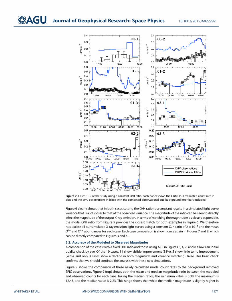
Figure 7. Cases 1–9 of the study using a constant O/H ratio, each panel shows the GUMCIS-4 estimated count rate inblue and the EPIC observations in black with the combined observational and background error bars included.
Figure 6 clearly shows that in both cases setting the O/H ratio to a constant results in a simulated light curvevariance that is a lot closer to that of the observed variance. The magnitude of the ratio can be seen to directlyaffect the magnitude of the output X-ray emission. In terms of matching the magnitudes as closely as possible,the modal O/H ratio from Figure 5 provides the closest match for both examples in Figure 6. We thereforerecalculate all our simulated X-ray emission light curves using a constant O/H ratio of 2 × 10⁻⁴ and the meanO7+ and O8+ abundances for each case. Each case comparison is shown once again in Figures 7 and 8, whichcan be directly compared to Figures 3 and 4.
5.2. Accuracy of the Modeled to Observed MagnitudesA comparison of the cases with a fixed O/H ratio and those using ACE in Figures 3, 4, 7, and 8 allows an initialquality check by eye. Of the 19 cases, 11 show visible improvement (58%), 5 show little to no improvement(26%), and only 3 cases show a decline in both magnitude and variance matching (16%). This basic checkconfirms that we should continue the analysis with these new simulations.
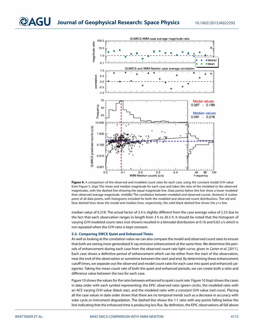
Figure 9 shows the comparison of these newly calculated model count rates to the background removedEPIC observations. Figure 9 (top) shows both the mean and median magnitude ratio between the modeledand observed counts for each case. Taking the median ratios, the minimum value is 0.38, the maximum is12.45, and the median value is 2.23. This range shows that while the median magnitude is slightly higher in
WHITTAKER ET AL. MHD SWCX COMPARISON WITH XMM-NEWTON 4171
Journal of Geophysical Research: Space Physics 10.1002/2015JA022292
Figure 8. Cases 10–19 of the study using a constant O/H ratio, each panel shows the GUMCIS-4 estimated count rate inblue and the EPIC observations in black with the combined observational and background error bars included.
ratio than the ACE varying modeled count rates, the range of the spread is much smaller. This can be seen bythe fact that 8 of the 19 case averages (42%) now sit within a factor of 2 higher or lower of the observationmagnitude average, two cases greater than the ACE O/H varying results (section 3.2). Figure 9 (middle) showsthe correlation value of the modeled and observed count rates. In comparison to the ACE varying data, themedian correlation is now 0.35 (compared to 0.07) with a standard deviation of 0.48 (compared to 0.52) and 5of the cases show negative correlation. This indicates that by removing the oxygen variation, we obtain muchbetter correlations between the model and observations. The median of the absolute value of correlation is0.57 (compared to 0.44), indicating that whether the case is positively or negatively correlated the variancesare more closely related with the O/H ratio kept constant.
Figure 9 (bottom) shows a scatterplot of each observed count rate bin against the respective modeled countrate for all cases. The scatterplot is accompanied by histograms of each count rate distribution. The solid blackline indicates an exact count rate match between observation and modeled count rates and, as expected bythe case average magnitude ratio of 2.23, most of the data points sit above this line. This is illustrated furtherby the red dashed lines which indicate the modal count rate bins; the EPIC modal value of 0.087 counts isapproximately half the modal GUMICS-4 count rate of 0.199. This approximate factor of two is duplicated inthe median of all data points (blue dashed line) where the EPIC value is 0.091 compared to the GUMICS-4
WHITTAKER ET AL. MHD SWCX COMPARISON WITH XMM-NEWTON 4172
Journal of Geophysical Research: Space Physics 10.1002/2015JA022292
Figure 9. A comparison of the observed and modeled count rates for each case, using the constant modal O/H valuefrom Figure 5. (top) The mean and median magnitude for each case and takes the ratio of the modeled to the observedmagnitudes, with the dashed line showing the equal magnitude line. Data points below this line show a lower modeledthan observed average magnitude. (middle) The correlation between modeled and observed counts. (bottom) A scatterpoint of all data points, with histograms included for both the modeled and observed count distributions. The red andblue dashed lines show the modal and median lines, respectively; the solid black dashed line shows the y=x line.
median value of 0.218. The actual factor of 2.4 is slightly different from the case average value of 2.23 due tothe fact that each observation ranges in length from 3 h to 26.5 h. It should be noted that the histogram ofvarying O/H modeled count rates (not shown) resulted in a bimodal distribution at 0.16 and 0.63 c/s which isnot repeated when the O/H ratio is kept constant.
5.3. Comparing SWCX Quiet and Enhanced TimesAs well as looking at the correlation value we can also compare the model and observed count rates to ensurethat both are seeing more generalized X-ray emission enhancement at the same time. We determine the peri-ods of enhancement during each case from the observed count rate light curve, given in Carter et al. [2011].Each case shows a definitive period of enhancement which can be either from the start of the observation,near the end of the observation or sometime between the start and end. By determining these enhancementcutoff times, we separate out the observed and model count rates for each case into quiet and enhanced cat-egories. Taking the mean count rate of both the quiet and enhanced periods, we can create both a ratio anddifference value between the two for each case.
Figure 10 shows the values for the ratio between enhanced to quiet count rate. Figure 10 (top) shows the casesin data order with each symbol representing: the EPIC observed ratio (green circle), the modeled ratio withan ACE varying O/H value (black star), and the modeled ratio with a constant O/H value (red cross). Placingall the case values in date order shows that there are no temporal trends such as a decrease in accuracy withsolar cycle or instrument degradation. The dashed line shows the 1:1 ratio with any points falling below theline indicating that the enhanced time is producing less flux. By definition, the EPIC observations all fall above
WHITTAKER ET AL. MHD SWCX COMPARISON WITH XMM-NEWTON 4173
Journal of Geophysical Research: Space Physics 10.1002/2015JA022292
Figure 10. The ratio between the enhanced and quiet charge exchange periods of the light curve. (top) The ratio forthe O/H varying model data (asterisk), O/H constant model data (cross), and the observed data (circle). These are indate order to determine any temporal bias. (bottom left) A scatterplot of O/H varying model data against the observeddata, with the red solid line showing the y=x line. The error bars on the observed data have been propagated fromthe background and observational data. Figure 10 (bottom right) shows the same plot but with the O/H constantdata points.
the ratio line with a mean increase of 48% and median increase of 22% in counts per second during SWCXenhancement times. The O/H varying cases have four cases where the ratio is less than 1, indicating that theSWCX enhanced period is returning less X-ray emission. Whereas for the constant O/H, there are only twocases where this occurs. The mean and median count rate increases for the O/H varying model are 370%and 53%, respectively. The equivalent values for the constant O/H model are 116% and 96%, respectively.While the varying O/H data provide a median increase between quiet and enhanced times similar to thatseen in the observed data, the extremely high mean value indicates that this is subject to high variation. Theconstant O/H ratio enhancement again shows a factor of 2 in both the mean and median enhancement rates.We investigate this further by plotting out each modeled enhancement ratio against the observed values inFigure 10 (bottom two panels). Figure 10 (bottom left panel) shows the ACE varying enhancement ratio, andFigure 10 (bottom right panel) shows the constant O/H enhancement ratio values, to be able to show bothdata sets on the same scale we have plotted these on a log x axis. The solid red line indicates the y=x linefor ease of comparison. The variability of the results can once again be seen in the ACE varying model dataalthough around the ratio of 1.5 the observations match up to the model extremely well. The constant O/Henhanced ratio values show a tighter spread but a reduced accuracy in the cases which matched well in thevarying O/H plot.
The ratio between enhanced and quiet times will be very sensitive to the quiet time magnitudes, which inturn will be heavily influenced by the calculated background values. As a complement to the ratio calcula-tion we have also determined the magnitude difference between enhanced and quiet times for each case,shown in Figure 11. Figure 11 (top) shows the difference values in time order, again showing no temporal pat-tern between observations and model results. The mean and median enhancements are 0.08 and 0.06 c/s forthe observed differences, 0.05 and 0.04 for the ACE varying model, and 0.15 and 0.09 for the constant O/H
WHITTAKER ET AL. MHD SWCX COMPARISON WITH XMM-NEWTON 4174
Journal of Geophysical Research: Space Physics 10.1002/2015JA022292
Figure 11. The difference between the enhanced and quiet charge exchange periods of the light curve. (top) The ratiofor the O/H varying model data (asterisk), O/H constant model data (cross) and the observed data (circle). These are indate order to determine any temporal bias. (bottom left) A scatterplot of O/H varying model data against the observeddata, with the red solid line showing the y=x line. The error bars on the observed data have been propagated from thebackground and observational data. (bottom right) The same plot but with the O/H constant data points.
model. Figure 11 (bottom) shows the scatterplot between observed and model differences; the solid red linein each plot shows the line of unity. Figure 11 (bottom left) also indicates the position of an outlying pointat a model difference value of −0.63 c/s; this has been shown in blue. The ACE varying data show a similarresult to Figure 10 with a few cases correlating very well to the observed differences, but the spread is widerthan the constant O/H model data. The data from both the difference and ratio between enhanced and quiettimes agree; in some cases the ACE varying data do an excellent job while setting the O/H ratio to constantproduces a more reliable result but reduces accuracy.
The case of 17 April 2002 (02-2) has no enhanced to quiet ratio for either O/H value, as the enhancementoccurs in the final two bins of the observation and neither simulation returns counts for this period.
5.4. Positional AccuracyAs a final piece of analysis we have also displayed the spatial position of the model data using a constant O/Hratio in Figure 12. Figure 12a shows the data in a cylindrical coordinate system (x-r) with the r axis signed bywhether the y value is positive or negative. This view gives us positional values projected onto a 2-D planewith a 0.5 RE by 1 RE resolution. We have binned all the data points and taken the average integral count ratefor each bin; with our limited number of case studies this leaves a large proportion of the grid without anydata but does show that the higher modeled count rates occur when the satellite is looking in the positive ydirection (dusk). Figure 12b shows the data binned in the y-z plane, with no dependence upon the x value.We can again observe the asymmetry in y, but the highest count rates occur at the z values closest to zero.As these values are likely to be closest to the nose of the magnetosheath it could simply be a proximity rela-tion to the highest emission rates. To determine whether distance from the magnetopause is significant, weplot each model count rate against the radial distance from the Shue magnetopause during the specific datapoint conditions. This scatterplot is shown in Figure 12c, with the data points split by y position. The positivey values are shown by black crosses, and the negative y values are shown by blue asterisks. When looking atall the data points combined, we can see that the count rate increases with distance from the magnetopause.
WHITTAKER ET AL. MHD SWCX COMPARISON WITH XMM-NEWTON 4175
Journal of Geophysical Research: Space Physics 10.1002/2015JA022292
Figure 12. The distribution of GUMICS-4 count rate distribution. (a) A cylindrical plot in the x-r plane with r signedby y showing the average modeled count rate in each bin, based on the position of XMM-Newton. (b) The countrates binned in the y-z plane. (c) A scatterplot showing the GUMICS-4 count rate values against distance from themagnetopause. (d) The correlation between GUMICS-4 and observations for each case plotted against the averagedistance from the magnetopause.
This result is initially counterintuitive, as we would expect the count rate to be higher the deeper in the mag-netosheath the satellite is. What must be considered is the pointing direction and case selection bias. A casewhere the satellite is far from the magnetopause would only have shown initial significant SWCX if the point-ing direction intersected a significant fraction of the magnetosheath. As the satellite comes closer to the Earththe integral path through the data grid includes fewer bins. If we took a sample of spacecraft positions withthe spacecraft pointing in random directions, then the opposite relation should be true. This magnitude plotshows, in a similar manner to the binned grid plots, that the count rates when y is positive are generally higher.Figure 12d shows average distance from the magnetopause with correlation between the observed and mod-eled light curves. These data points are again split by whether y is positive or negative. There appears to be nogeneral pattern between light curve variance and magnetopause distance, although the highest correlationsoccur in the negative y value (dawn) data values. This asymmetry was also mentioned in Carter et al. [2011],where they found that the empirical model fitted better in the dawnside. This dawn-dusk asymmetry couldbe related to the known asymmetries in either the magnetosheath plasma conditions [e.g., Walsh et al., 2012]or magnetopause position [e.g., Dmitriev et al., 2004], indicating that this asymmetry needs to be consideredduring the modeling process.
6. Conclusions
In this study we have taken the data from 19 case studies using the EPIC-MOS instruments on XMM-Newton toexamine the accuracy of MHD modeling when describing solar wind charge exchange from the Earth’s mag-netosheath. We found that a large amount of variation in the modeled light curve was caused by variationsin the oxygen to hydrogen ratio and abundances of oxygen charge states. In a large number of these casessetting the oxygen to hydrogen ratio to a constant improved the variance matching. These modeled data val-ues with a constant O/H ratio and mean charge state abundances were then compared to the observed lightcurves, providing an average correlation value of 0.35. This correlation has been reduced by the fact that 5 ofthe 19 cases are anticorrelated. The average magnitude ratio is a factor of 2.4 when averaging across all datapoints, giving 42% of the cases having an average magnitude within a factor of 2 of the observed data values,
WHITTAKER ET AL. MHD SWCX COMPARISON WITH XMM-NEWTON 4176
Journal of Geophysical Research: Space Physics 10.1002/2015JA022292
a slight decrease on the empirical method used in Carter et al. [2011]. The highest modeled count rates occurwhen the satellite is in the positive GSE y, with the highest correlations arising in negative y (dawn).
It is clear from sections 4.2 and 5 that the oxygen data inputs to the MHD model include substantial errors. TheO/H variances cause large changes in the modeled light curves which are simply not seen in the observed lightcurves for a significant number of cases. The longer (temporally) the case is, the more likely that a constant O/Hratio is inappropriate, yet accurate data are needed. The same applies to the oxygen charge state abundances;the 2 h resolution of this data is low for modeling that runs at a 4 s calculation resolution and a 5 min gridoutput. The absolute abundance values themselves are also an issue; it is unknown what the upper and lowerlimits of O7+ and O8+ should be. We observed in Figure 5 that the O7+ abundance can take a wide rangeof values, up to 52% which is likely unphysical. It is certain that the values given in Schwadron and Cravens[2000], while of the right order of magnitude, are of limited use for this particular modeling, especially as theydescribe almost no highly charged states in the fast wind. To improve on model accuracy, we either requiremore accurate and numerous solar wind oxygen observations closer to the Earth or an accurate proxy such asan extension of the proton entropy correlation work by Pagel et al. [2004] to include the O8+/O7+ ratio. Usinga constant value for the O/H ratio of 2×10⁻⁴ and mean oxygen charge states for each case, we have removeda large amount of this variation at the cost of a small accuracy loss (e.g., Figures 10 and 11).
The accuracy of the MHD modeling ranges from anticorrelated to an excellent correlation. We can link severalof the errors in both magnitude and variance to the oxygen data and the disparity of the MHD magnetopauseposition to the Shue model. The other data inputs to the MHD model behave well, and we have some excel-lent comparisons as seen in Figures 7 and 8. When comparing the MHD model to the empirical model usedin Carter et al. [2011], we can say that it performs equally well. The slight decrease of magnitude matching,42% rather than 50%, of cases within a factor of 2, could easily be due to the background removal. Decreas-ing the background removal values by 0.03 c/s actually increases the magnitude comparison accuracy to 63%hence showing the importance of the background removal when we look at comparing the magnitudes. Thebackground removal does not affect the correlation or the enhanced to quiet differencing comparison how-ever. Examining the magnitude difference between quiet and enhanced periods, we see very similar resultsbetween the observed values and the MHD model. The difference in the dawn-dusk correlations, also seenin Carter et al. [2011], suggests that there could be an asymmetrical process affecting the charge exchangeemission magnitude, which is missing from both models.
Users wishing to estimate the near-Earth SWCX values are advised that using either the empirical model or anMHD model with constant solar wind oxygen parameters is equally likely to produce a useable value. Whencomparing enhanced to quiet times, i.e., taking an average over a longer time period, using the variable O/Hdata is likely to be a valid approach. For those interested in a more in depth view of what is happening in termsof global SWCX around the Earth, the MHD-based model with a constant oxygen ratio and abundances, willproduce a more accurate result, including matching short timescale emissivity variation. This study also actsas a validation of the model methodology for global imaging of the magnetosheath using SWCX, by providingsimilar emissivities to observed values. However, the relative inaccuracy of using a far upstream monitor forthe solar wind conditions can affect the model results considerably. This modeling will be especially importantfor future missions involving wide angle X-ray imaging of the Earth’s magnetosheath.
ReferencesBailey, J., and M. Gruntman (2011), Experimental study of exospheric hydrogen atom distributions by Lyman-alpha detectors on the TWINS
mission, J. Geophys. Res., 116, A09302, doi:10.1029/2011JA016531.Bodewits, D. (2007), Cometary X-rays. Solar wind charge exchange in cometary atmospheres, PhD thesis, Univ. of Groningen, Netherlands.Carter, J. A., and A. M. Read (2007), The XMM-Newton EPIC background and the production of background blank sky event files,
Astron. Astrophys., 464, 1155–1166, doi:10.1051/0004-6361:20065882.Carter, J. A., and S. Sembay (2008), Identifying XMM-Newton observations affected by solar wind charge exchange - Part I, Astron. Astrophys.,
489(2), 837–848, doi:10.1051/0004-6361/200809997.Carter, J. A., S. Sembay, and A. Read (2010), A high charge state coronal mass ejection seen through solar wind charge exchange emission
as detected by XMM-Newton, Mon. Not. R. Astron. Soc., 402, 867–878, doi:10.1111/j.1365-2966.2009.15985.x.Carter, J. A., S. Sembay, and A. Read (2011), Identifying XMM-Newton observations affected by solar wind charge exchange—Part II,
Astron. Astrophys., 527, A115, doi:10.1051/0004-6361/201015817.Collier, M. R., T. E. Moore, M.-C. Fok, B. Pilkerton, S. Boardsen, and H. Khan (2005), Low-energy neutral atom signatures of magnetopause
motion in response to southward Bz, J. Geophys. Res., 110, A02102, doi:10.1029/2004JA010626.Collier, M. R., D. G. Siebeck, T. E. Cravens, I. P. Robertson, and N. Omidi (2010), Astrophysics noise: A space weather signal, Eos Trans. AGU,
91(24), 213–214, doi:10.1029/2010EO240001.Collier, M. R., et al. (2012), Prototyping a global soft X-ray imaging instrument for heliophysics, planetary science, and astrophysics science,
AcknowledgmentsThis research used the ALICE/SPECTREHigh Performance Computing Facilityat the University of Leicester. TheGUMICS-4 MHD code is provided bythe Finnish Meteorological Institute,while the simulation runs arestored on the HPC facilities atthe University of Leicester. TheOMNI solar wind data were takenfrom NASA’s GSFC/SPDF repository(omniweb.gsfc.nasa.gov). The ACEsolar wind composition data weretaken from the ACE Science Centerwww.srl.caltech.edu/ACE/ASC/.The background countrates were calculated usingthe WebPIMMS service(heasarc.gsfc.nasa.gov/cgi-bin/Tools/w3pimms/w3pimms.pl).Effort sponsored by the Air ForceOffice of Scientific Research, AirForce Material Command, USAF,under grant FA9550-14-1-0200. TheU.S. Government is authourized toreproduce and distribute reprintsfor Governmental purposes notwith-standing any copyright notationthereon. J.A.C. and S.E.M. gratefullyacknowledge support from the STFCconsolidated grant ST/K001000/1.
WHITTAKER ET AL. MHD SWCX COMPARISON WITH XMM-NEWTON 4177
Journal of Geophysical Research: Space Physics 10.1002/2015JA022292
Collier, M. R., et al. (2014), On lunar exospheric column densities and solar wind access beyond the terminator from ROSAT soft X-rayobservations of solar wind charge exchange, J. Geophys. Res. Planets, 119, 1459–1478, doi:10.1002/2014JE004628.
Cravens, T. E. (1997), Comet Hyakutake X-ray source: Charge transfer of solar wind heavy ions, Geophys Res. Lett., 24, 105–109,doi:10.1029/96GL03780.
Cravens, T. E. (2000), Heliospheric X-ray emission associated with charge transfer of the solar wind with interstellar neutrals,Astrophys. J., 532, L153, doi:10.1086/312574.
Cravens, T. E., I. P. Robertson, and S. L. Snowden (2001), Temporal variations of geocoronal and heliospheric X-ray emission associated withthe solar wind interaction with neutrals, J. Geophys. Res., 106(A11), 24,883–24,892, doi:10.1029/2000JA000461.
Dennerl, K. (2008), X-rays from Venus observed with Chandra, Planet. Space Sci., 56(10), 1414–1423, doi:10.1016/j.pss.2008.03.008.Dimmock, A. P., K. Nykyri, H. Karimabadi, A. Osmane, and T. I. Pulkkinen (2015), A statistical study into the spatial distribution and dawn-dusk
asymmetry of dayside magnetosheath ion temperatures as a function of upstream solar wind conditions, J. Geophys. Res. Space Physics,120, 2767–2782, doi:10.1002/2014JA020734.
Dmitriev, A. V., A. V. Suvorova, J. K. Chao, and Y.-H. Yang (2004), Dawn-dusk asymmetry of geosynchronous magnetopause crossings,J. Geophys. Res., 109, A05203, doi:10.1029/2003JA010171.
Gordeev, E., G. Facskó, V. Sergeev, I. Honkonen, M. Palmroth, P. Janhunen, and S. Milan (2013), Verification of the GUMICS-4 global MHDcode using empirical relationships, J. Geophys. Res. Space Physics, 118, 3138–3146, doi:10.1002/jgra.50359.
Henley, D. B., and R. L. Shelton (2008), Comparing Suzaku and XMM-Newton observations of the soft X-ray background: Evidence for solarwind charge exchange emission, Astrophys. J., 676, 335, doi:10.1086/528924.
Hodges, R. R., Jr. (1994), Monte Carlo simulation of the terrestrial hydrogen exosphere, J. Geophys. Res., 99(A12), 23,229–23,247,doi:10.1029/94JA02183.
Holmström, M., S. Barabash, and E. Kallio (2001), X-ray imaging of the solar wind-Mars interaction, Geophys. Res. Lett., 28(7), 1287–1290,doi:10.1029/2000GL012381.
Hosokawa, K., S. Taguchi, S. Suzuki, M. R. Collier, T. E. Moore, and M. F. Thomsen (2008), Estimation of magnetopause motion fromlow-energy neutral atom emission, J. Geophys. Res., 113, A10205, doi:10.1029/2008JA013124.
Hubert, B., M. Palmroth, T. V. Laitinen, P. Janhunen, S. E. Milan, A. Grocott, S. W. H. Cowley, T. Pulkkinen, and J-C. Gérard (2006),Compression of the Earth’s magnetotail by interplanetary shocks directly drives transient magnetic flux closure, Geophys. Res. Lett., 33,L10105, doi:10.1029/2006GL026008.
Ishikawa, K., Y. Ezoe, Y. Miyoshi, N. Terada, K. Mitsuda, and T. Ohashi (2013), Suzaku observation of strong solar-wind charge-exchangeemission from the terrestrial exosphere during a geomagnetic storm, Publ. Astron. Soc. Jpn., 65(3), 63, doi:10.1093/pasj/65.3.63.
Janhunen, P., M. Palmroth, T. Latinen, I. Honkonen, L. Juusola, G. Facskó, and T. I. Pulkkinen (2012), The GUMICS-4 global MHDmagnetosphere-ionosphere coupling simulation, J. Atmos. Sol. Terr. Phys., 80, 48–59, doi:10.1016/j.jastp.2012.03.006.
Jansen, F., et al. (2001), XMM-Newton observatory: I. The spacecraft and operations, Astron. Astrophys., 365, L1–L6,doi:10.1051/0004-6361:20000036.
Kalberla, P. M. W., W. B. Burton, D. Hartmann, E. M. Arnal, E. Bajaja, R. Morras, and W. G. L. Pöppel (2005), The Leiden/Argentine/Bonn(LAB) Survey of Galactic HI. Final data release of the combined LDS and IAR surveys with improved stray-radiation corrections,Astron. Astrophys., 440(2), 775–782, doi:10.1051/0004-6361:20041864.
King, J. H., and N. E. Papitashvili (2005), Solar wind spatial scales in and comparisons of hourly Wind and ACE plasma and magnetic fielddata, J. Geophys. Res., 110, A02104, doi:10.1029/2004JA010649.
Koutroumpa, D. (2012), Update on modeling and data analysis of heliospheric solar wind charge exchange X-ray emission, Astron. Nachr.,333, 341–346, doi:10.1002/asna.201211666.
Kuntz, K. D., and S. L. Snowden (2008), The EPIC-MOS particle induced background spectra, Astron. Astrophys., 478(2), 575–596,doi:10.1051/0004-6361:20077912.
Kuntz, K. D., Y. M. Collado-Vega, M. R. Collier, H. K. Connor, T. E. Cravens, D. Koutroumpa, F. S. Porter, I. P. Robertson, D. G.Sibeck, and S. L. Snowden (2015), The solar wind charge-exchange production factor for hydrogen, Astrophys. J., 808(2), 143,doi:10.1088/0004-637X/808/2/143.
Liemohn, M. W., J. U. Kozyra, V. K. Jordanova, G. V. Khazanov, M. F. Thomsen, and T. E. Cayton (1999), Analysis of early phase ring currentrecovery mechanisms during geomagnetic storms, Geophys. Res. Lett., 26(18), 2845–2848, doi:10.1029/1999GL900611.
Lisse, C. M., et al. (1996), Discovery of X-ray and extreme ultraviolet emission from Comet C/Hyakutake 1996 B2, Science, 274(5285),205–209, doi:10.1126/science.274.5285.205.
Milan, S. E., S. W. H. Cowley, M. Lester, D. M. Wright, J. A. Slavin, M. Fillingim, C. W. Carlson, and H. J. Singer (2004), Response of themagnetotail to changes in the open flux content of the magnetosphere, J. Geophys. Res., 109, A04220, doi:10.1029/2003JA010350.
Nass, H. U., J. H. Zoennchen, G. Lay, and H. J. Fahr (2006), The TWINS-LAD mission: Observations of terrestrial Lyman-𝛼 fluxes,Astrophys. Space Sci. Trans, 2, 27–31, doi:10.5194/94JA02183.
Ogasawara, K., V. Angelopoulos, M. A. Dayeh, S. A. Fuselier, G. Livadiotis, D. J. McComas, and J. P. MCFadden (2013), Characterizing thesayside magnetosheath using energetic neutral atoms: IBEX and THEMIS observations, J. Geophys. Res. Space Physics, 118, 3126–3137,doi:10.1002/jgra.50353.
Østgaard, N., S. B. Mende, H. U. Frey, G. R. Gladstone, and H. Lauche (2003), Neutral hydrogen density profiles derived from geocoronalimaging, J. Geophys. Res., 108(A7), 1300, doi:10.1029/2002JA009749.
Pagel, A. C., N. U. Crooker, T. H. Zurbuchen, and J. T. Gosling (2004), Correlation of solar wind entropy and oxygen ion charge state ratio,J. Geophys. Res., 109, A01113, doi:10.1029/2003JA010010.
Palmroth, M., T. I. Pulkkinen, P. Janhunen, and C.-C Wu (2003), Stormtime energy transfer in global MHD simulation, J. Geophys. Res., 108(A1),1048, doi:10.1029/2002JA009446.
Palmroth, M., I. Honkonen, A. Sandroos, Y. Kempf, S. von Alfthan, and D. Pokhotelov (2013), Preliminary testing of global hybrid-Vlasovsimulation: Magnetosheath and cusps under northward interplanetary magnetic field, J. Atmos. Sol. Terr. Phys., 99, 41–46,doi:10.1016/j.jastp.2012.09.013.
Powell, K. G., P. L. Roe, T. J. Linde, T. I. Gambosi, and D. L. de Zeeuw (1999), A solution-adaptive upwind scheme for idealmagnetohydrodynamics, J. Comput. Phys., 154(2), 284–309, doi:10.1006/jcph.1999.6299.
Robertson, I. P., and T. E. Cravens (2003), Spatial maps of heliospheric and geocoronal X-ray intensities due to the charge exchange of thesolar wind with neutrals, J. Geophys. Res., 108(A10), 8031, doi:10.1029/2003JA009873.
Robertson, I. P., M. R. Collier, T. E. Cravens, and M.-C. Fok (2006), X-ray emission from the terrestrial magnetosheath including the cusps,J. Geophys. Res., 111, A12105, doi:10.1029/2006JA011672.
Schwadron, N. A., and T. E. Cravens (2000), Implications of solar wind composition for cometary X-rays, Astrophys. J., 554, 558–566.
WHITTAKER ET AL. MHD SWCX COMPARISON WITH XMM-NEWTON 4178
Journal of Geophysical Research: Space Physics 10.1002/2015JA022292
Shue, J. H., et al. (1998), Magnetopause location under extreme solar wind conditions, J. Geophys. Res., 103(A8), 17,691–17,700,doi:10.1029/98JA01103.
Slavin, J. D., B. J. Wargelin, and D. Koutroumpa (2013), Solar wind charge exchange emission in the Chandra deep field north,Astrophys. J., 779(1), 13, doi:10.1088/0004-637X/779/1/13.
Snowden, S. L., M. R. Collier, and K. D. Kuntz (2004), XMM-newton observation of solar wind charge exchange emission, Astrophys. J., 610(2),1182–1190, doi:10.1086/421841.
Spreiter, J. R., A. L. Summers, and A. Y. Alksne (1966), Hydromagnetic flow around the magnetosphere, Planet. Space Sci., 14, 223–250,doi:10.1016/0032-0633(66)90124-3.
Strüder, L., et al. (2001), The European photon imaging camera on XMM-Newton: The pn-CCD camera, Astron. Astrophys., 365, L18–L26,doi:10.1051/0004-6361:20000066.
Turner, M. J. L., et al. (2001), The European photon imaging camera on XMM-Newton: The MOS cameras, Astron. Astrophys., 365, L27–L35,doi:10.1051/0004-6361:20000087.
Voges, W., et al. (1999), The ROSAT all-sky survey bright source catalogue, Astron. Astrophys., 349(2), 389–405.Walsh, B. M., D. G. Sibeck, Y. Wang, and D. H. Fairfield (2012), Dawn-dusk asymmetries in the Earth’s magnetosheath, J. Geophys. Res., 117,
A12211, doi:10.1029/2012JA018240.
WHITTAKER ET AL. MHD SWCX COMPARISON WITH XMM-NEWTON 4179


![JournalofGeophysicalResearch: SolidEarth · PROOF Journal of Geophysical Research: Solid Earth 10.1002/2015JB012604 [Kováacsetal.,2012].Sincethefocusofthepresentstudyisontheuppermantle](https://static.documents.pub/doc/80x56/5f0b4dd97e708231d42fdad9/journalofgeophysicalresearch-solidearth-proof-journal-of-geophysical-research.jpg)