Norwegian School of Economics Bergen, December, 2015 Modeling the Steel Price for Valuation of Real Options and Scenario Simulation Master thesis in Finance Norwegian School of Economics Written by: Lasse Berggren Supervisor: Jørgen Haug This thesis was written as a part of the Master of Science in Economics and Business Administration at NHH. Please note that neither the institution nor the examiners are responsible — through the approval of this thesis — for the theories and methods used, or results and conclusions drawn in this work.
Transcript
Norwegian School of EconomicsBergen, December, 2015
Modeling the Steel Price forValuation of Real Options and
Scenario Simulation
Master thesis in Finance
Norwegian School of Economics
Written by: Lasse Berggren
Supervisor: Jørgen Haug
This thesis was written as a part of the Master of Science in Economics and BusinessAdministration at NHH. Please note that neither the institution nor the examinersare responsible — through the approval of this thesis — for the theories and methodsused, or results and conclusions drawn in this work.
1
Summary
Steel is widely used in construction. I tried to model the steel price such that valuationsand scenario simulations could be done. To achieve a high level of precision this isdone with a continuous-time continuous-state model. The model is more precise than abinomial tree, but not more economically interesting. I have treated the nearest futuresprice as the steel price. If one considers options expiring at the same time as the futures,it will be the same as if the spot were traded. If the maturity is short such that detailslike this matters, one should treat the futures as a spot providing a convenience yieldequal to the interest rate earned on the delayed payment. This will in the model bethe risk-free rate.
Then I have considered how the drift can be modelled for real world scenario simu-lation. It involves discretion, as opposed to finding a convenient AR(1) representation,because the ADF-test could not reject non-stationarity (unit root).
Given that the underlying is traded in a well functioning market such that pricesreflect investors attitude towards risk, will the drift of the underlying disappear in theone-factor model applied to value a real-option. The most important parameter for thevaluation of options is the volatility. I have estimated relative and absolute volatility.The benefit of the relative volatility is the non-negativity feature.
Then I have estimated a model where the convenience yield is stochastic. Thishas implications for the risk-adjusted model. I have difficulties arriving at reliableparameter estimates. Here small changes in arguments have large effects on the optionvalue. Therefore should this modelling be carried through only if one feels comfortablethat it is done properly.
I finish by illustrating how real-option valuation can be performed. The trick is totranslate the real-world setting into a payoff function. Then one can consider MonteCarlo simulation if the payoff function turns out to be complicated or if there aredecisions to be made during the life of the project. For projects maturing within thehorizon traded at the exchange, the expectation of the spot price under the pricingmeasure is observable.
To truly compare models, plots of the value of derivative should be created tographically compare the difference in dependence on parameter values. Alternatively,the derivative of the expressions with respect to the parameters are compared. Thevalue of the option to do something, as opposed to be committed to do something,increases with the volatility of future outcomes. Such known results are used insteadin the comparison, because the two reliable models (the one-factor models) are prettysimilar. This known result is not contradicted by the present values computed in thereal option example.
Motivation for this thesis Steel is a central input factor in a variety of construction
projects. Such projects typically extend far into the future and has associated exposure
to price changes. Thus, to understand and identify a model for the dynamics of the
steel price is interesting for scenario simulations, computing the value of an insurance
and for valuations of the option to act in a particular way during projects, i.e. real
options in projects.
In which situations is this useful? Consider a construction company involved with
a skyscraper and the nearby metro. They want to get an overview of their exposure
to price fluctuations in one of their input factors, steel, and manage this risk. How do
they achieve risk management?
Consider a shipyard building ships. A major input factor in the construction process
is steel. The supplier of steel adjust the price charged to the shipyard to cover its varying
expenses. The shipyard is therefore exposed to steel price fluctuations. Assume that
the shipyard wants an insurance against high prices. What is the fair price of the
insurance?
Consider a steel supplier with a planned production level two years into the future.
What is the value of the option to increase production in the event of a high price?
How will I answer these questions? I will identify and calibrate models for the
steel price that incorporate time and uncertainty. I will apply what is known as risk-
neutral valuation when the task is to compute present values.
Part II:
Steel
6
7 2. Global Steel Markets
2 Global Steel Markets
China plays a key role. The Economist (2015, 9Dec) 1 reports that China produced
822 million metric tonnes in 2014, about half the worlds annual output. China is pre-
dicted (late 2015) to produce over 400 million metric tonnes more than it will consume
in 2015.2 China has of November exported over 100 million metric tonnes. To compare
these numbers, Japan produce roughly 110 metric tonnes3, while US produced about
90 million metric tonnes in 2014.4 Financial Times (2015)5 report that as of 2014, the
volume on the Shanghai Futures Exchange is larger than the London Metal Exchange
and Commodity Exchange, Inc (New York) aggregated.
3 Characteristics of Steel
Steel is cheap and has high tensile strength. It can take on a great variety of
forms and is widely used in construction, offshore installations and shipbuilding. The
properties depends on the particular alloy and the particular production process. Steel
can be recycled without loosing its quality — it is the most recycled material in the
world.6 Scrap metal is back in the market after three months.
Steel is cheap to store and transport. Cheap storage leads to stable production
for storage — it is more cost effective to produce and store it than to constantly adjust
produced output. Warehouses also works as a buffer for shocks in demand, dampen-
ing price volatility. Cheap storage costs reduce the difference in prices between steel
delivered far in the future and steel delivered soon.
Steel is durable. Steel in warehouses does not degrade, so situations where con-
sumers are unwilling to delay consumption should be rare. That is, situations in which
futures contracts with short maturity are more expensive than longer contracts with
longer maturity, should be rare.
1The Economist Newspaper Ltd: ”China’s soaring steel exports may presage a trade war”, Dec 9th2015. ”Nervousness of steel”, Sep 19th 2015, ”It’s a steel”, Jul 13th 2015
2Reuters: ”China apparent steel consumption falls 5.7 pct from Jan-Oct -CISA”, Nov 13th 2015.3The Japan Iron and Steel Federation, Review 2015, http://www.jisf.or.jp/en/statistics/
sij/documents/P02_03.pdf4Profile 2015. American Iron and Steel Institute.5http://www.ft.com/intl/cms/s/0/a2df3018-9feb-11e4-9a74-00144feab7de.html#
axzz3ukMbHj006Profile 2015. American Iron and Steel Institute.
Steel compared to other commodities Steel is easy and cheap to store as opposed
to gold, oil and in particular electricity. Steel production is not dependent on weather
as coffee and oranges are. It is also easier to regulate steel production than cattle
production on short notice. Steel is consumed, contrary to silver and gold. Steel is
durable as opposed to seasonal commodities. Steel is recycled as opposed to live cattle.
9 4. Rebar to Represent Steel in General
4 Rebar to Represent Steel in General
The steel price Steel is used all over the world and it is not clear what the steel price
is. There exists several steel price indexes trying to represent a particular type of steel
or a geographical area. There are also steel futures prices on different steel products.
A futures contract is a contract traded on an exchange and standardized with respect
to type, quality, location, and maturity for future delivery of the underlying. The
underlying is in this case steel. Rebar is the most traded metal futures contract in the
world, with 408 million contracts in 2014.7 Futures prices are easy to interpret because
the steel can in fact be delivered to the quoted price. Also, because the prices are on
contracts traded on an exchange as opposed to the indices, the prices can be used as
an instrument in cash flow management.
Based on the large role of China, and the fact that the SHFE steel futures contracts
are relatively new, do I choose to focus on steel in China and use futures contracts traded
on the Shanghai Futures Exchange to represent the steel price. I will in particular focus
on rebar futures contracts.
What is rebar? Rebar is short for reinforcement bar, and is used in concrete con-
structions. Concrete has high compression strength but low tensile strength. Steel is
therefore used as reinforcement.
Why Rebar? Rebar is the most traded futures contract and should be the best
reflection of the steel price in China and Asia. 8 Companies involved with other steel
products like wire rod and hot-rolled coil, find the dynamics of rebar interesting as rebar
contracts can be used to cross-hedge. Cross-hedging is to hedge your direct exposure
to price volatility in X by trading a sufficiently correlated product Y. The correlations
of rebar versus different related products, given that they are cointegrated:9
- Wire Rod SHFE 98% for F2.10
7The Financial Times Limited, Commodities Explained: Metals trading in China, April 2nd 20158Volumes: http://www.csidata.com/factsheets.php?type=commodity&format=html&
exchangeid=56. On the arbitrary day 1 December, rebar had 350 times (9,194,734/26,300)higher volume than hot-rolled coil while steel wire rod were not even traded. On Decemeber 12, rebarvolume were 3,228,720, hot-rolled coil 14,742 and steel wire rod not traded.
9F2 contracts matures between 1 month and 2 months, F4 matures between 3 and 4 months, astime passes. I have chosen the shortest maturity available. E.g. Nickel F4 because F1, F2, F3 hadshorter time series. The correlation is similar for all maturities for Wire Rod SHFE and Hot RolledCoil SHFE.
- Hot Rolled Coil NYMEX F1 79%, F2 83%, F3 86%, F4 88%.13
- Iron Ore (62% Fe, CFR China) NYMEX 97% for F2.14
Cross-hedging is typically done if the trading volume (i.e. liquidity) is low in the
product you have direct exposure in. Liquidity is important to be able to take the
desired hedging positions at any time.
11Sample period: 27 Mar 2015-21 Sept 2015.12Sample period: 21 Mar 2014-21 Sept 2015.13Sample period: 05 Jan 2010-21 Sept 2015. Observe how the correlation rises with maturity, likely
due to the geographical differences between the exchanges.14Sample period: 05 Jan 2010-21 Sept 2015.
11 5. Data Description
5 Data Description
Rebar Futures Contracts Traded on Shanghai Futures Exchange
(SHFE)
Contract specifications The contracts are traded in yuan, while the data set is in
dollar. I have daily observations on ten futures contracts, maturing up to ten months.
Rebar contracts are physically settled each month. Delivery must take place within five
days after the last trading day.15 The fee is one yuan per metric ton for physical delivery.
Minimum Delivery Size is 300 metric tonnes, each contract is on 10 metric tonnes.
Certified warehouses are located in Shanghai, Jiangsu (near Shanghai), Guangzhou
(near Hong Kong) and Tianjin (near Beijing). For detailed contract specifications, see
the appendix on page 80.
Futures Prices The yuan price of the nearest rebar futures contract and the one
with the longest maturity, 10 months, are graphed in Figure 2(a). The negative price
trend in many commodities over recent years applies to steel as well. The number of
observations per different contract maturity is 211.
15Last trading day: 15th, or first trading day following 15th
12 5. Data Description
Figure 1: Rebar Futures Prices on Shanghai Futures Exchange in yuan and dollar in(a) and (b), the exchange rate used to convert is in (c). January 2010 - September2015.
2010 2011 2012 2013 2014 2015
2000
2500
3000
3500
4000
4500
5000
YUAN P
ER CO
NTRACT
FUTURES(1) YuanFUTURES(10) Yuan
(a) Yuan denominated rebar futures prices F0,1 and F0,10.
2010 2011 2012 2013 2014 2015
300
400
500
600
700
800
US DOL
LAR PE
R CONT
RACT
FUTURES(1) US DollarFUTURES(10) US Dollar
(b) Dollar denominated rebar futures prices F0,1 and F0,10.
2010 2011 2012 2013 2014 2015
6.2
6.4
6.6
6.8
YUAN P
ER US
DOLLAR
(c) Yuan per US Dollar exchange rate.
13 5. Data Description
Volatility Define relative volatility per week as σw = std.dev[ln(Ft/Ft−1)] and abso-
lute volatility per week as γw = std.dev[Ft − Ft−1]. To annualize, multiply by√
52.
In Figure 2 is the annualized relative volatility associated with the different maturities
plotted and both relative and absolute volatilities are tabulated.
Rebar futures prices with short maturity are more volatile to than those with longer
maturities. This is referred to as the Samuelson effect, stating that the arrival of new
information has more impact on short maturity contracts than long maturity contracts.
Figure 2: Annualized relative and absolute volatility associated with the different ma-turities of the rebar contracts. Contract one has from one month to 0 days maturity astime passes, contract two has two to one month maturity and so on.Relative: σann = std.dev [ln(Ft/Ft−1)]×
√52.
Absolute: γann = std.dev[Ft − Ft−1]×√
52
●
●
●
●
●
●
●
●
●●
2 4 6 8 10
0.18
0.19
0.20
0.21
0.22
0.23
0.24
1 2 3 4 5 6 7 8 9 10
ANNU
ALIZ
ED R
ELAT
IVE
VOLA
TILIT
Y
MATURITY OF REBAR FUTURES CONTRACTS
Contract Annualized Volatility
Relative Absolute
1 23.83 % 794 Yuan
2 20.29 % 728 Yuan
3 18.88 % 705 Yuan
4 17.86 % 676 Yuan
5 18.25 % 685 Yuan
6 18.54 % 708 Yuan
7 19.08 % 733 Yuan
8 18.12 % 691 Yuan
9 18.52 % 709 Yuan
10 18.31 % 708 Yuan
14 5. Data Description
Figure 3: Relative volatility through time for F0,1 and F0,10. The horizontal bandsrepresents one standard deviation on a weekly frequency.
2010 2011 2012 2013 2014 2015
−0.10
−0.05
0.00
0.05
0.10
RELAT
IVE VO
LATILIT
Y
lnF(1)_t − lnF(1)_t−1 lnF(10)_t − lnF(10)_t−1
Figure 4: Absolute volatility through time for F0,1 and F0,10. The horizontal bandsrepresents one standard deviation on a weekly frequency.
2010 2011 2012 2013 2014 2015
−300
−200
−100
0
100
200
300
ABSO
ULUT
E VOL
ATILIT
Y
F(1)_t − F(1)_t−1 F(10)_t − F(10)_t−1
15 5. Data Description
The kurtosis associated with the distribution of returns for commodities is typi-
cally16 above 3, meaning that it has fatter tails than the normal distribution. The
normal distribution is nevertheless often, and will also here be, the main tool in mod-
elling the stochastic price process. Often, a separate jump process is added in models
for prices that jumps, rather than widening the distribution. The distribution of log
returns in Figure 6(a) appears normal and it is not obvious that the absolute changes
are log-normally distributed in Figure 6(b). The distribution appear to be wider in
Figure 6(b).
Figure 5: The computed kurtosis shows that the distributions has fatter tails than thenormal distribution, but is considerably less than what Geman (2005) reports. Seefootnote 16.
−0.15 −0.10 −0.05 0.00 0.05 0.10 0.15
0.00
0.05
0.10
0.15
0.20
ln(F1(t+1)) − ln(F1(t))
PRO
BABI
LITY
OF
OBS
ERVI
NG
TH
E R
ETU
RN
KURTOSIS = 4.54
ST.DEV = 0.03305
(a) Distribution of the percentage return of the
rebar price.
−400 −200 0 200 400
0.00
0.05
0.10
0.15
0.20
F1(t+1) − F1(t)
PRO
BABI
LITY
OF
OBS
ERVI
NG
TH
E R
ETU
RN
KURTOSIS = 3.78
ST.DEV = 110.08
(b) Distribution of the absolute change of the
rebar price.
16Geman (2005), page 59 calculates kurtosis, from July 1993 to November 2000, here written compactwith no decimals: Crude oil 6, Brent 6, Natural gas 30, Heating fuel 11, Unleaded gasoline 4, Corn 51,Soybeans 19, Soymeal 15, Soy oil 5, Wheat 59, Oats 23, Coffee 7, Aluminium 6, Copper 7, Zinc 12,Nickel 5, Tin 6 Lead 6.
16 5. Data Description
Term structure of the futures prices Basis is defined as a longer maturity contract
minus a shorter maturity contract (or the spot price), e.g. Ft,10−Ft,1 . Define the relative
basis as the difference in the log-prices. The relative basis is displayed in Figure 6 for
ln(Ft,10/Ft,1) and ln(Ft,5/Ft,1). A positive value is known as “contango” and a negative
value is known as “backwardation”. Define the futures term structure as the curve
observed when the prices observed at date t for futures contracts maturing at different
dates are plotted with the maturity of the contract on the horizontal axis and the
price on the vertical axis. Contango is lingo to describe a situation where the futures
term structure is upwards sloping, and backwardation is a name for when the slope
is neqative. The term structure of the futures prices can possibly add information on
price dynamics.
There are cost-of-carry associated with possessing steel physically, which in the
absence of other effects make the futures curve slope upwards. Backwardation can be
regarded as a situation where agents are unwilling to delay consumption, or a situation
where sellers give up a portion of the price to achieve certainty of the future price
instead. I have included ln(Ft,5/Ft,1) in Figure 6 to shed light on the shape of the
futures curve. The futures curve can be hump shaped and need not be monotonically
increasing or monotonically decreasing as the graph hints towards. The graph hints
towards monotonically increasing term structure because ln(Ft,5/Ft,1) is for the most
part below ln(Ft,10/Ft,1) in the figure. The number of cases in which both the shorter
maturity and longer maturity contracts were more expensive than the middle contract
is as follows, F2: 27, F3: 28 F4: 34, F5: 45, F6: 41, F7: 40, F8: 35, F9: 34. Per
contract series are there 211 observations.
Figure 6: Relative basis. January 2010 - September 2015. Positive: Contango. Neg-ative: Backwardation. Relative basis can also be regarded as a measure of “cost-of-carry”.
2010 2011 2012 2013 2014 2015
−0.2
−0.1
0.0
0.1
0.2
RELATIV
E BASI
S
ln(F10) − ln(F1)ln(F5) − ln(F1)
Inventories The theory of storage summarized: Low warehouse stock leads to higher
nearby futures prices and higher volatility. The price versus stock at the warehouse is
plotted in Figure 7. A linear regression equation to estimate the fit does not improve
casual inspection in this case. The data do not confirm a relationship as predicted by
the theory of storage. Volatility is somewhat higher for lower inventory levels, seen
in Figure 8(b). The obvious shortcoming in the data is that it is for the warehouses
associated with the SHFE only. Buyers and sellers can easily stock steel at their sites,
in addition to deliver to the exchanges, so producers and consumers easily influence
observable inventory level analysed here. The expectation of a relationship vanish as a
result of the shortcoming. The lack of relation is demonstrated here because inventory
data could easily come to mind as a possible source of information for modelling prices.
Figure 7: Rebar warehouse exchange stock versus price level and volatility.
●●●●●●●●
●
●●●
●●●●
●
●
●
● ●●
●●●
●
●●
●
●●
●●
●●● ●●
●●●●●●
●
●●
●
●●
●
●
●
●
●●●●
●●
●
●
● ●●
●
●●●●
●● ● ●●●●●●
●●●●●●●●●●
●
●●●●
●
●● ● ●
●
●
●
●
●
●
●●
●●● ●
● ● ●
●●
●●
2000 2500 3000 3500 4000
0
20000
40000
60000
80000
100000
120000
REBAR PRICE IN YUAN (t)
REBA
R W
AREH
OUSE
STO
CK (t
)
(a) The relationship in levels is weak with a correlation of - 0.2.
●● ●● ●●●●
●
●
●● ●
●● ● ●
●
●
●
●●●●
● ●●
●●
●
●●
●●
●● ●●● ●● ●
● ●●●
●●
●
●●
●
●
●
●
● ●●●
●●
●
●
●●●
●
● ● ●●
● ● ●●● ●●●●
● ●● ● ●●●
●●●
●
●●
●●
●
● ●●●
●
●
●
●
●
●
●●
●● ●●
● ●●
● ●
●●
−0.10 −0.05 0.00 0.05 0.10
0
20000
40000
60000
80000
100000
120000
ln(R1(t+1)) − ln(R1(t))
0.041
0.035
0.032
0.036
STANDARDDEVIATION
REBA
R W
AREH
OUSE
STO
CK(t)
(b) Percentage change in price over a week given warehouse stock in t.
One standard deviation indicated by grey boxes. Sample period: July
2012 to September 2015.
17
Part III:
Modelling I:
General Considerations
18
19 6. General Modelling Considerations
6 General Modelling Considerations
Computing a present value.
The present value of a certain future cash flow takes the time value of money into
account by discounting with a risk-free interest rate. When there are associated uncer-
tainty, the present value is affected. To compute the present value, assumptions must
be made, often via an explicit model. A common way is to model the uncertainty going
forward with real probabilities and then add a premium — reflecting the risk associated
with the expected outcome — to the risk-free rate when discounting the future value
back to a present value. An alternative way is to model the uncertainty going forward
with artificial probabilities and then use only the risk-free rate to discount back into a
present value. This is referred to as “risk-neutral valuation”. Both approaches involves
setting up a model reflecting the relevant economy and use parameter values in the
computation. I will use risk-neutral valuation. Risk-neutral valuation is explained in
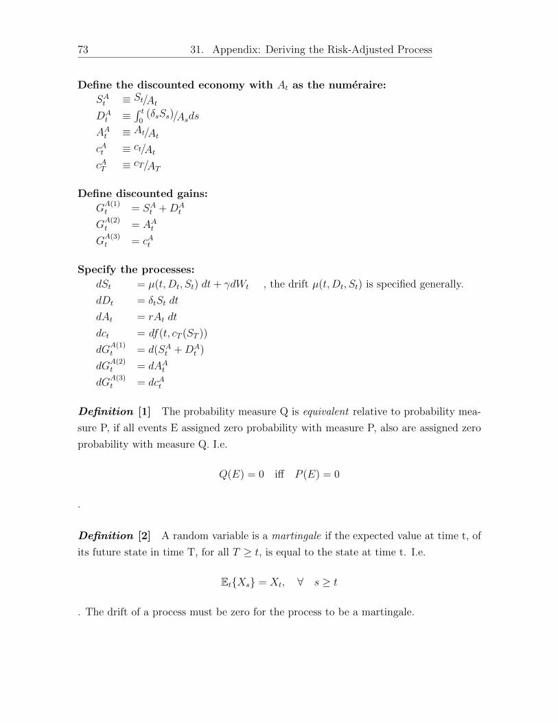
Appendix: Deriving the Risk-Adjusted Process on page 72.
Model of uncertainty.
The simplest model of uncertainty and time is one in which a variable takes on a value
today and can only take on two different values in the next time period — a binomial
model. This specification is reasonable to model a coin flip, but not to model the steel
price, because the steel price can take on more than two values and uncertainty is
considered over more than one period ahead. To model the steel price, the binomial
model can be extended by adding the binomial structure to it self for each of the two
possible outcomes, resulting in a “tree”. Doing this n times results in a tree with
n+ 1 different possible outcomes if the tree does not keep track the specific path taken
through the tree. In this discrete model, a reasonable fine outcome grid for a fixed
future time period can be constructed by increasing n. To be completely precise in the
modelling, one can construct a mathematical object that moves continuously through
time and can take on a continuous set of values. The exchange has trading hours, so
the price is not traded continuously. The price quotations are not continuous either,
rather they are quoted in fixed intervals, e.g. yuan per ton. The continuous time can
be thought of as what the price would have been, if it were traded in the closing hours.
The continuous outcome space will ‘fit’ every discrete version, and is easier to scale
in time while preserving precision. The benefit of continuous-time, continuous-set of
values lies in the precision of the model and importantly, not in the economic principles
20 6. General Modelling Considerations
and intuition.
Stochastic differential equation (SDE) to model uncertainty and
time
I will consider SDE’s that consists of a drift term and a dispersion term.
dXt = µ(t,Xt)× dt+ σ(t,Xt)× dWT
change in XT = (drift function)× dt+ (dispersion function)× randomness
Drift takes care of the deterministic part of the change, while the dispersion term takes
care of stochastic part. The stochastic ‘motor’ is the Wiener process. Both the drift and
dispersion can be functions of the stochastic variable and time. Hull (2015) is sufficient
to be able to work with SDE’s, Øksendal (1998) is more rigorous. When dealing with
SDE’s normal calculus does not apply, rather Ito calculus must be applied. I have
stated Ito’s formula in Appendix: Ito’s Formula on page 56 because it is used later.
Modelling implications from economic theory
Existing producers have the possibility to regulate production and supply in response
to the steel price, thus the quantity in the market should be a function of the price.
The price should be driven down by producers when the price is high. When the price
is low, supply is expected to decrease and some firms forced out of business if the low
price persists — eventually the price moves up again. Demand is also a source of mean-
reversion, because a high price makes it more attractive to use substitute materials,
decreasing steel demand. Similarly steel is more attractive when it is cheap, increasing
demand. This economic reasoning implies that a property of the drift function should
be that it makes sure that the process mean-reverts.
The fundamental value of the steel price is likely to change with the improvements
in production technology and prices of input factors. The prices of the input factors,
demand and supply are likely a function of the economical environment in a broad sense.
Hence, it is not obvious how to model the level for which the process seeks to return to.
An alternative is to identify the relationship between some key variables, and use that to
orient on whether the current price is above or below what is historically observed as the
(cointegrated) relationship. If the interest rate is a proxy for the state of the economy,
it could be allowed to vary in the model. The interest rate observed at the Peoples
Bank of China has been around 5% from 2010 to 2015. I will use a constant interest
21 7. Particular Modelling Considerations
rate of 5% throughout my work. Trading it self will induce price fluctuations, so the
prices will be an imperfect measure of fundamentals. Using a constant interest rate also
simplify away the interest effect for margin payments on futures contracts (adjustment
of your cash balance in the broker account on a daily basis to avoid inability to meet
your obligations).
I argue that when the purpose of modelling is to characterize dynamics for subse-
quent simulation, the source of the random movements is not critical as long as the
model reflects the characteristics of the price movements. The purpose in this thesis
is not to predict the direction of the future movements of the steel price, although a
prediction on the direction is an implication of a process that mean-reverts.
7 Particular Modelling Considerations
Yuan versus dollar
The contracts are traded in yuan, while the price series are in dollars. I want to
model the steel price process in Shanghai from an independent geographical perspec-
tive. Therefore, to avoid measurement noise by dollar-yuan fluctuations I convert the
observations back into yuan via daily observations of the currency pair accessed at the
webpage of the St.Louis Fed.17 The rebar prices in dollar and the exchange rate used
is seen in Figure 2(b) and 2(c).
Sample period
In the time period considered, the prices declines. One must be careful with the inter-
pretation of the data. In any case the history is just a particular realization of possible
outcomes. If the prices did not have any tendency to increase nor decline, it would be
tempting to assume a constant simple mean as the equilibrium price. It would possibly
be the statistical equilibrium price, i.e. the mean over the period, but the true equilib-
rium is a function of economic activity and the costs of production. Hence, to evaluate
the equilibrium level, I argue that there are two options: (i) Industry knowledge about
production costs and predicted demand, (ii) Statistical approach is to consider vari-
ables that are likely to be co-integrated with rebar. A few candidates are iron ore,
Daily observations on trading days are not equidistant with respect to calendar time,
but could be with respect to the flow of relevant information.18 Daily observations
increase the sample size, and there is some evidence that increased frequency for a
given sample size increase the power when testing for unit root, but the time span is
considered to be more important.19
I choose to use a weekly frequency motivated by, (i) no need to distinguish between
calendar time and abstract information flow time. Annually expressed time step will be
1/52. (ii) Unit root test are not adversely affected. (iii) The fact that the construction
sector plan and act with a long time perspective, and are not interested in micro
dynamics. If one wants to investigate micro dynamics, a daily frequency is likely to
be too infrequent anyway. (iv) A weekly frequency is common in the literature, e.g.
Schwartz (1997).
18If observations are equidistant with respect to relevant information, it means that relevant in-formation is not three times as large over a weekend (three nights) than for example Wednesday toThursday (one night). The arrival of relevant information induces price changes, i.e. volatility. Hence,relevant information flow is tested by comparing volatilities over a night versus over three consecutivenights where there were no trading.
19E.g. Page 130 in Maddala and Kim (2004)
22
Part IV:
Modelling II:
One Factor Model
23
24 8. One Factor Model
8 One Factor Model
Mean-Reverting Model With Absolute Volatility The economics of steel mar-
kets call for mean-reversion in the model, although there is reasonable doubt when
eye-balling figure 2(a). In Figure 3 and 4 it is seen that the volatility is not necessarily
proportional to the price. When price changes are proportional to the price level, the
distrubution of the prices will be log-normal and the percentage return will be normal.
I choose the main model to be one where the volatility is absolute.
Based on this do I suggest the mean-reverting Orhnstein-Uhlenbeck process for the
futures price level:
dFt,T = κ (µ− Ft,T ) dt+ γdWt (1)
Mu µ is the long run mean of Ft,T . If Ft,T > µ, the deterministic drift term is
negative. Because the term is negative when Ft,T > µ, and positive when Ft,T < µ,
the process mean-reverts. The deviation from the mean is scaled by kappa κ. Thus
the speed of reversion is determined by κ. This deterministic part of the process is
disturbed by a random variable Wt, and scaled by a parameter gamma γ. The random
variable Wt is the standard Wiener process.20
Ft,T can become negative, not consistent with the price of a commodity. If the mean
is sufficiently far away from zero and the mean-reversion is strong, this is unlikely.
Discrete version The discrete version of (1) with time step ∆t is
Ft+∆t,T − Ft,T = κ (µ− Ft,T ) ∆t+ γ√
∆t ηt+∆t , where ηt+∆t ∼ ηt ∼ N(0, 1) (2)
This version could be used to estimate parameters if the analytical solution were difficult
to find. If this form is used, the size of the time increment ∆t is important. Solving (1)
analytically is preferable because the discrete version will be exact for all choices for
the size of ∆t.21 When estimating parameters in a later section, the analytical solution
will be used and the chosen weekly frequency implies ∆t = 1/52.
20Properties of the standard Wiener process: W0 = 0, Wt−Ws ∼ N(0, t−s) where s ≤ t, incrementsof Wt −Wt−1,Wt−1 −Wt−2, ... are independent of one another, Wt is the sum of its increments andWt is continuous but not differentiable.
21See Appendix: The (Possible) Role of ∆t on page 55 for an illustration of the role of ∆t.
25 8. One Factor Model
Analytical solution The analytical solution is22
FT,T = Ft,T e−κT + µ
(1− e−κT
)+ γ
∫ T
t
eκ(s−T )dWs (3)
FT,T is a random variable because of the presence of the stochastic integral. The
expectation and variance at t for date T are:
E{FT,T} = Ft,T e−κT + µ
(1− e−κT
)(4)
V ar (FT,T ) = γ2
∫ T
t
e2κ(s−T )ds (5)
Mean-Reverting Model With Relative Volatility This model cannot become
negative in the continuous case. One has to take care in an Euler scheme here as well,
because the system is not updated over ∆t. If the distance ∆t is large, the system is
not updated frequently enough to sufficiently scale down the dispersion term.
dFt,T = κ (µ− Ft,T ) dt+ σFt,TdWt (6)
22See Appendix: Solving the Mean-RevertingOrnstein–Uhlenbeck Process on page 57 for a detailed way to the solution.
26 9. Estimation, One Factor Model
9 Estimation, One Factor Model
Estimate an AR(1)
I now turn to Box-Jenkins methodology.
Strategy The discrete version of (3) with a time step ∆t is
Ft+∆t,T = Ft,T e−κ∆t + µ
(1− e−κ∆t
)+ γ
√1− e−2κ∆t
2κηt+∆t , ηt+∆t ∼ N(0, 1) (7)
AR(1) with non-zero mean:
yt = a0 + a1yt−1 + εt , εt ∼ N(0, σ2
)(8)
The estimation strategy is to equate:
yt =Ft+∆t,T (9)
a0 =µ(1− e−κ∆t
)(10)
a1 =e−κ∆t (11)
yt−1 =Ft,T (12)
sd.err(ε) =γ
√1− e−2κ∆t
2κ(13)
and solve for µ, κ and γ using the computed numbers for a0, a1 and sd.err(ε), to
obtain:
κ =− ln a1
∆t(14)
µ =a0
1− a1
(15)
γ =sd.err(ε)
√−2 ln a1
∆t(1− a21)
(16)
Testing the underlying assumptions A condition for estimating the linear model,
is that the process is stationary. To test for stationarity, I employ an Augmented Dickey-
Fuller test23 without drift or trend. The idea is to test the true data generating process,
23See appendix on Augmented Dickey Fuller test on page 51
27 9. Estimation, One Factor Model
and not fit an equation to the observed sample in the testing. I do not want to allow for
a trend or drift in the test, because it is not theoretically compatible with the price of
a commodity. In fact, a positive trend reflecting inflation could be present, but in the
sample the general tendency is a decreasing price. Although the production process is
likely to be cost-improved over time, the price cannot decrease in a deterministic nor
in an average fashion forever. Hence, I do not allow for a trend or drift. Interestingly,
if the prices had an overall tendency to increase, it would be tempting to reason that it
is for example inflation or a stable growth in demand, and include drift in the testing
equation. If prices follow mean-reversal along an upward sloping trend it would be
reasonable to include a trend.
The ADF test statistic for F1 is -1.16, not even significant at the 10% level24. Hence,
the process is not proven to be stationary. This means that the numbers a0, a1, sd.err(ε)
in (10), (11), (13) cannot be reliably computed and plugged into the expressions for
κ, µ, γ in (14), (15), (16).
Hence, either the price reverts slowly towards the mean, or it is a true unit root
process. Over a short time horizon a true unit root and a near unit root are similar,
and they appear more similar the larger the volatility is. ADF test and other unit root
tests are known to have low power, so it is not good in differentiating a near unit root
from a true unit root.
When failing to reject unit root In general, when one wants to identify a pattern
and predict the future, but fail to reject unit root, one must identify whether detrending
or differencing is the proper method to make it stationary, and proceed. Differencing
results in working with ARIMA(p,1,q), rather than ARIMA(p,0,q). ARIMA(p,1,0) is
on the form ∆yt =∑p
i=1 ∆yt−i. I can report that a1 is insignificant in ARIMA(1,1,0),
so there is no predictive pattern in such a simple model. Using ARIMA(0,1,0) as the
model of the mean, I reject conditional variance by testing the squared forecasting
errors with the Ljung-Box test and McLeod Li test.25 This is true for ARIMA(1,1,0)
as well.
To take the first difference is not compatible with (1) and (3), because (1) and
(3) describe a change from t to T based on the level in t. The aim is not to predict
the future, but to find parameters for (1) and (3), with the restriction to keep it in
levels. Now, there are two options. (i) Do not take the difference, but assume unit
24Critical values, given sample size and test regression specification without drift or trend are -2.58,-1.95, and -1.62, for significance levels 1%, 5%, and 10% respectively. Test statistics computed are F1:-1.16, F10
25See subsection in on page 53 for an informal explanation.
28 10. Assume Unit Root
root. (ii) Use discretion on the reversal. This implies setting the speed of reversion κ
and long term mean µ to values such that the process mean reverts and are consistent
with the failure of rejecting unit root. The low power of the unit root test could be
used to argue that a higher value of kappa is also consistent with mean-reversal and
failure to reject unit root.
10 Assume Unit Root
Cannot reject unit root for AR(1), so assume that the coefficient a1 is one. Because
a1 = 1, I impose a0 = 0 or else the process has a deterministic trend.
yt = a0 + yt−1 + εt , εt ∼ N(0, σ2
)(17)
yt = yt−1 + εt (18)
The solution to (18) is26
yt = y0 +t−1∑i=0
εt−i (19)
This is known as a random walk. Each new realization of the innovation εt has a
permanent effect on yt+s, so the process is not stationary, but finite because of the given
initial value y0 and terminal time t.
Model implication To equate this with the mean-reverting process described by (1)
and (3) implies a drift of zero, by setting κ = 0. The mean-reversal property vanishes,
as already pointed out by the fact that the series is not stationary. The continuous
model with is thus
dFt,T = γdWt (20)
FT,T = Ft,T + γ
∫ T
t
dWs (21)
The discrete version of (20) is
Ft+∆t,T = Ft,T + γ√
∆t ηt+∆t , ηt+∆t ∼ ηt ∼ N(0, 1) (22)
26See Appendix: Solve AR(1), a0 = 0 and a1 = 1 on page 54 for the derivation.
29 11. Use Discretion On The Drift
The discrete version of (21) is
FT,T = Ft,T + γ√
(T − t) ηT , ηT ∼ ηt ∼ N(0, 1) (23)
(22) and (23) are similar because they are now nothing more than an initial condition
plus a scaled draw from the standard normal distribution. They are analoge to (19),
the difference is that εt ∼ N (0, σ2) and ηt ∼ N (0, 1), so γ is needed in (22) and (23)
to take care of the scaling of the volatility.
The absoulte annualized volatility γ is computed in Figure 2 to be 794 yuan. The
last observation in the sample is 1900 yuan, so the lower bound in a two standard
deviation confidence interval equals 1900 − 2 × 794 = 312. It is clear that this model
can take on negative values. Negative values will not be observed in reality, so this a
drawback with this model.
11 Use Discretion On The Drift
Before even discussing the speed of reversal to the long run mean level, the long run
mean level must be determined. It can be constant or time-varying, and the relevant
time horizon must be determined. The mean can also be constant or time-varying based
on industry and production knowledge.
The average price of F1 from January 2010 to September 2015 is 3638 yuan. The
average for September 2014 to September 2015 is 2295 yuan. Does it matter what the
price were 5 years ago? These are clearly discretionary considerations. Iron ore (also
integrated of order one) and rebar are cointegrated. They are cointegrated because the
residuals ut, from a linear regression of the type Rebart = a + b × Iron oret + ut are
stationary. If the residuals are not stationary, then there are no a and b to transform
from one variable to the other that will be correct in expectation. The last observation
for iron ore is 347 yuan, and 1900 yuan for rebar. The OLS estimate and these values
gives 1900 − 1052 + 3.3 × 347 = u, u = −297. Because the error is negative, it means
that they are closer than they have been historically, and they should therefore diverge.
30 11. Use Discretion On The Drift
Figure 8: Iron ore and rebar are cointegrated, because the residuals from a regressionis stationary. It implies that OLS is valid, and that this relationship is the averagetransformation from one to the other.
2010 2011 2012 2013 2014 2015
−600
−400
−200
0
200
400
600
RESID
UAL
RESIDUAL = REBAR − 3.3 X IRON ORE − 1052
(a) The residual from a linear regression. When it is negative, it means that they are closer than they
have been on average historically, and therefore should diverge in the future.
2010 2011 2012 2013 2014 2015
1000
2000
3000
4000
5000
YUAN
(b) The dotted line is the prediction of rebar based on iron ore. At the end of the sample, it predict a
higher value for rebar than the realized value. The relation in the regression could have been specified
the other way around, because there are no explainatory intentions, just a linear relationship. One
must remember that there are no information on which variable that is going to move in a particular
direction. The information here is that they will diverge, but one can only use this information in a
relative sense, not to undertake level predictions.
31 12. Convenience Yield
12 Convenience Yield
Another possible source of information is the term structure of futures prices. A simple
relation between two futures prices is27
Ft,T = Ft,ser(T−s) , t < s < T. (24)
This relation states that you move through the term structure of futures prices via
the constant interest rate r and the time distance T − t. This is violated empirically.
It is seen in Figure 2(a) that the distance between the prices do not obey this relation.
Introducing a varying convenience yield δt (expressed as a rate) is the standard way
to treat the empirical discrepancy between the futures prices (e.g. Schwartz (1997),
Cassusus and Collin-Dufresne (2005)).
Definition of convenience yield, Schwartz (1997) page 927, footnote 9,
The convenience yield can be interpreted as the flow of services accruing to
the holder of the spot commodity but not to the owner of a futures contract.
With deterministic convenience yield, (24) is modified to
Ft,T = Ft,se(r−δs,T )(T−s) , t < s < T. (25)
The convenience yield is analogue to a dividend yield (rate) on a stock. If the
convenience yield is negative, it is sometimes referred to as cost-of-carry — the cost
of storing the commodity is paid by the party possessing the commodity and not the
holder of the contract. I solve for the convenience yield in (25) to obtain
δt,s,T =r −(
1
T − s
)ln
(Ft,TFt,s
), t < s < T
and use the particular contracts F1 and F10 to plot the empirical convenience yield as
a residual in Figure 9. The convenience yield is stationary (ADF-test statistic is -3.95).
27See the paragraph preceeding (60) on page 79 for why the relation is as it is.
Figure 9: Convenience yield. Annualized convenience yield as a residual δANN = 43δ1,10
where δ1,10 = 0.05− 43ln(F0,10
F0,1
), obtained from the commonly assumed relation between
futures prices: Ft,T = Ft,se(r−δs,T )(T−s) , t < s < T . January 2010 - September 2015.
2010 2011 2012 2013 2014 2015
−0.3
−0.2
−0.1
0.0
0.1
0.2
0.3
CONV
ENIEN
CE Y
IELD
13 Summary One Factor Model
Mean-reversal in the drift term is not supported by the employed statistical ADF-
test to check for stationarity. The test is known to be weak in disentangling near
unit root and true unit root processes. The importance of the distinction decreases
with a decreasing horizon. I have shown the implications for the model under Assume
Unit Root on page 28. If one really wants to incorporate a drift that is not zero,
I have suggested discretionary ways. Possibilities are, setting kappa directly, using
cointegration to update the changing mean level and use convenience yield that depends
on the spot price.
32
Part V:
Modelling III:
Two Factor Model
33
34 14. Motivation for Stochastic Convenience Yield
14 Motivation for Stochastic Convenience Yield
As the two futures contracts in (25) are stochastic, it is interesting to allow for it in
the model. Then at least r or δ must be allowed to vary. Schwartz (1997) and Collin-
Duffresne (2005) shows how a mean-reverting convenience yield significantly matters
for pricing of contingent claims.
According to the theory of storage, is the convenience yield related to the economy
wide inventory levels. When the inventory is low, rebar is scarce so the price and
the volatility should rise. The volatility rises because the price sensitivity to changes
in demand when the inventory is low, is larger. Furthermore, the importance of low
inventory is more important for the immediate future than for a longer horizon. The
flow of information should in general be more important for the immediate future.
Hence, the nearby futures prices should have a higher volatility than the longer maturity
futures.
15 Modelling an Unobservable Variable
I now estimate a model for the unobservable spot price, by taking the whole futures
curve into consideration. Because the underlying variable is unobservable, it must first
be estimated. To do this the log futures prices are put in a state-space form so that
the Kalman-filter28 and Maximum Likelihood Estimation29 can be used to estimate the
time series of the spot price and the associated model parameters.
Schwartz (1997) adds noise to his data to reflect bid-ask spreads, and non-simultaneously
observed variables, price limits or errors in the data and then use the Kalman-filter to
filter out this noise. The aim is that the serial correlation and cross-correlation is a
result of variation in the spot price and convenience yield. I do not add noise to my
prices.
28See Appendix: Kalman Filter on page 68 for an informal explanation.29See Appendix: Maximum Likelihood Estimation on page 69
35 16. Theoretical Model
16 Theoretical Model
In this part I will impose the two-factor model (26) (27) (28) developed in Schwartz and
Gibson (1990) and extended in Schwartz (1997) on the rebar futures data. The rebar
spot price follows a mean-reverting geometric Brownian motion. The convenience yield
is a variant of the mean-reverting Ornstein-Uhlenbeck process, similar in structure as
(1). There are now two sources of randomness driving the two SDE’s, with correlation
ρ.
Historical measure:
dSt =(µ− δt)St dt+ σSSt dWSt (26)
dδt =κ (α− δt) dt+ σδ dWδt (27)
dW δt dW
St =ρdt (28)
The model under the historical measure is the version used for scenario simula-
tion.30 There is an modified version of this used to compute present values — the
risk-neutral valuation tool.31. I present the modified model used for pricing here for
completeness. It is then clear where the risk-adjustment λδ for the non-traded risk
factor convenience yield seen in the estimations belong. The model under the pricing
measure is represented by (29) (30) (31).
Pricing measure:
dSt =(r − δt)Stdt+ σSSt dW St (29)
dδt = [κ (α− δt)− λδσδ] dt+ σδ dW δt (30)
W δt W
St =ρ dt (31)
17 Estimation Strategy
To fit the Two-Factor Model to the rebar data I have used the function fit.schwartz2f
in the package Schwartz97 avaiable at the Comprehensive R Archive Network (CRAN).
It employs the Kalman filter technique to estimate the state variable—the unobservable
spot price, which then enables Maximum Likelihood Estimation in order to find optimal
To the optimization function I provide what I will refer to as “settings”:
• A matrix of weekly observations of one to ten month futures contracts, and specify
the time increment to be 1/52.
• A matrix of days to maturity for each contract
• Which parameters to be optimized and which to be held constant
• Initial values of the parameters
• A constant interest rate of 5%
• All maturities receive the same weight in the estimation of the spot price.
. The estimation procedure is unfortunately not as simple as one function call with the
“settings” above. The output from the optimization function is sensitive to initial val-
ues. Further, there exists local paths where two parameter values can increase pairwise
to values not desirable from a modelling perspective (e.g. σδ = sigmaE = 6 × 10153
is not what I want to plug into my model). Therefore, to test the robustness of the
estimates do I need to vary the settings in a number of ways. In addition to vary the
initial values, it is recommended to vary which parameters to be fixed and which to be
optimized. A more detailed description with illustrations and a comparison of different
parameter-sets are in Appendix: Two-Factor Model Robustness test on page 59.
18 Estimation Results
In Table 1, I present the results of the estimations. The results presented are based on
a corrected mean of the values in the filtrated matrix shown in Figure 12 and 13. The
filtrated matrix consists only of vectors of parameter values where all parameters are
estimated to be within discretionary filter limits.
37 18. Estimation Results
Table 1: Estimated parameters for the Two-Factor Model. Filtering: Numbers arebased on a filtered list of vectors. For each vector in a list of returned vectors from aparameter optimization function, only returned vectors where all parameter values areinside its respective limits are stored in the filtered list of returned vectors. Correcting:The mean is computed over the observations where the parameter were in fact free tovary, i.e. the constant parts seen in figure 12 and 13 are not included in the computationof the mean. Vectors with some parameters constant are included in the filtered list ofvectors because the other parameters vary, and contribute with observations to computetheir means.
Filter Limits
Parameters Mean Std.dev Low High
mu µ 0.1899 0.1704 0.001 1
sigmaS σS 0.3421 0.134 0.001 5
kappaE κ 12.4609 4.997 5 30
alpha α 0.2995 0.1366 0.001 5
sigmaE σδ 2.1907 1.1217 0.001 5
rhoSE ρSδ 0.9886 0.0124 0.9 1
lambdaE λδ 3.7291 1.7689 0.001 10
Some estimated parameter values are strange. The correlation of 98% is very high.
Also the drift in the real world mu is estimated to be 19%. A relative volatility of
34% is reasonable, but it does not agree with the relative volatility calculated in the
one-factor model. By setting up an Euler scheme it is easy to investigate properties
of the model. The stationary level to which the convenience yield converts to is −0.35
under the pricing measure. This is means that the net convenience yield is negative.
This is not surprising because the term structure of the futures curve is upwards sloping
for the most part. The level of kappa implies that if the convenience yield is either 0 or
-0.7, it takes two months before it is close to -0.35 (-0.39 and -0.31) and three months
to reach -0.36 and -0.34. While the negative sign on the convenience yield long run
level is expected, the level is low.
38 18. Estimation Results
Figure 10: Simulated convenience yield over 26 weeks. The convenience yield has amuch higher volatility than observed in the real world data in Figure 9.
0 5 10 15 20 25
−2.0
−1.0
0.00.5
1.0
WEEKS
SIMUL
ATED C
ONVE
NIENC
E YIEL
D
Figure 11: Simulated steel price under the pricing measure. The positive trend ingeometric brownian motion is clear.
0 20 40 60 80 100
2000
3000
4000
5000
6000
WEEKS
SIMUL
ATED S
TEEL
PRICE
39 18. Estimation Results
Figure 12: The filtrated matrix of acceptable values of µ, σs, κ. The mean is computedover the observations where the parameter were in fact free to vary, i.e. the constantparts are not included in the computation of the mean. N is the sample size for whichthe mean and standard deviation are computed.
0 1000 2000 3000 4000
0.0
0.2
0.4
0.6
0.8
1.0
FUNCTION CALLS
mu
MEAN
=
0.1899
ST.DEV
=
0.1704
N
=
398
1
(a) µ
0 1000 2000 3000 4000
0.0
0.5
1.0
1.5
FUNCTION CALLS
sigmaS
MEAN
=
0.3421
ST.DEV
=
0.134
N
=
310
5
(b) σs
0 1000 2000 3000 4000
5
10
15
20
25
30
FUNCTION CALLS
kappaE
MEAN
=
12.4609
ST.DEV
=
4.997
N
=
398
6
(c) κ
40 18. Estimation Results
Figure 13: The filtrated matrix of acceptable values of α, σδ, ρSE, λδ. The mean iscomputed over the observations where the parameter were in fact free to vary, i.e. theconstant parts are not included in the computation of the mean. N is the sample sizefor which the mean and standaard deviation are computed.
0 1000 2000 3000 4000
0.0
0.2
0.4
0.6
0.8
1.0
FUNCTION CALLS
alpha
MEAN
=
0.2995
ST.DEV
=
0.1366
N
=
398
5
(a) α
0 1000 2000 3000 4000
0
1
2
3
4
5
FUNCTION CALLS
sigmaE
MEAN
=
2.1907
ST.DEV
=
1.1217
N
=
340
1
(b) σδ
0 1000 2000 3000 4000
0.90
0.92
0.94
0.96
0.98
1.00
FUNCTION CALLS
rhoSE
MEAN
=
0.9886
ST.DEV
=
0.0124
N
=
297
8
(c) ρSE
0 1000 2000 3000 4000
0
2
4
6
8
FUNCTION CALLS
lambda
E
MEAN
=
3.7291
ST.DEV
=
1.7689
N
=
340
0
(d) λδ
Part VI:
Application
41
42 19. Application
19 Application
For the risk-neutral valuation framework, see Appendix: Deriving the Risk-Adjusted
Process on page 72.
Real Options At the date a futures contract has delivery, it is effectively a spot price.
For an option maturing at this date, it will be the same whether you evaluate an option
on the futures or the spot. If they do not expire on the same date, but lets say by a two
week difference, one can treat the option on the futures contract as a stock paying a
dividend yield and, set the yield to the risk-free rate. This reflects the delayed payment
of the futures. Alternatively, if the option expires sufficiently far in the future, e.g. two
years, there will be other sources of uncertainty more important than this small detail.
E.g. constant interest rate over the two years. The trick with real option valuation is
the translation of the real world problem into a derivative interpretation, i.e. a cash
flow function must be specified. The option to expand production is a call option on
the underlying. If there is a continuous decision considerations in reality, it will be an
American option rather than European, complicating the valuation. Also, one must
remember that risk-neutral valuation relies on the assumption that the prices reflects
risk preferences. For steel, the futures contracts are traded in well functioning markets,
the exchange, so I rely on the risk-correction using this technique. In comparing the
models, examples are really not necessary, because it is known that a greater volatil-
ity increases the option value. Hence, a model which mean-reverts under the pricing
measure will yield lower prices than the model with unbounded variance. When the
volatility is absolute, the volatility gives the option a higher value the lower the spot
price. I will here present an example to illustrate how real option pricing theory can
be used, rather than to highlight key differences between the models.
Scenario Simulation For scenario simulation the ‘real world dynamics’ are used.
Complicated cases can be evaluated based on how the single processes ends up. These
processes yield a distribution for the many paths simulated, thereby giving a measure
on the uncertainty of the future outcomes. Here, caution has to be paid to whether
there are correlations between the variables that should be taken into account in the
simulation.
43 19. Application
Option to expand production
The numbers are inspired by accounting figures from a large Chinese steel maker.
Consider a steel manufacturer who have predicted that optimal production level is
Q1 = 46 million metric tonnes in two years. r = 5%. The current steel price
is 1900 yuan. They have agreed on terms of delivery with its suppliers, fixing the
unit input costs to 0.9 of the current steel price plus. In addition 6,000 million
yuan covers plants, financial capital and administration expenses. This amounts to
1, 900 × 0.9 × 46m + 6, 000m = 84, 660m yuan. The present value of this project if
there is no convenience yield is like a forward contract. In particular, if the project
where inside 10 months, the expected steel price under the pricing measure would be
observable at the exchange. For a two year horizon the present value is
Schwartz, Eduardo S. ”The Stochastic Behavior of Commodity Prices: Implications
for Valuation and Hedging.” The Journal of Finance: 923.
Øksendal, B. K. Stochastic Differential Equations: An Introduction with Applica-
tions. 5th ed. Berlin: Springer, 1998.
Part IX:
APPENDICES
50
51 23. Appendix: ADF-test
23 Appendix: ADF-test
The problem Consider the AR(p) model,
yt = α1yt−1 + . . .+ αpyt−p + εt , εt ∼ N(0, σ2
). (32)
The problem is that if the coefficients in the true data generating process (DGP) sum
to one, the series exhibit unbounded variance.32 Unbounded variance is a violation of
one ordinary least squares (OLS) assumption, so using OLS to model the true DGP
will not yield reliable results.
Unit root. If the sum of the coefficients sum to one, at least one characteristic root
is unity, referred to as unit root.
Consider the simpler case of eq. (32) with p = 1,
yt = α1yt−1 + εt (33)
here, unit root corresponds with α1 = 1 so eq. (33) becomes
yt = yt−1 + εt (34)
In (34) new realizations of εt, called innovations, have a permanent effect on all future
values of the series. This is why the variance is unbounded. In equation (34) the
expected value of the series for an arbitrary future date is the current level of the series.
It implies that the history of the sequence is not useful in predicting the future direction
of the sequence. The contrary case is if α1 6= 1. If |α1| > 1 the process will explode. If
|α1| < 1 the process will revert to a long term mean. When |α1| < 1, the value of yt is
by it self useful in predicting the future direction of the sequence, because the process
will revert to its mean in the absence of shocks. The smaller α1 is, the faster will the
series revert to the mean.
Ordinary critical t-values cannot be used to test whether α1 6= 1. Dickey-Fuller
critical values are needed.
32Almost one is almost unbounded variance, as the system will be very slow to revert to the mean.
52 23. Appendix: ADF-test
The Augmented Dickey-Fuller test
The cautionary way to test α1 is to assume α1 = 1, and try to reject the assumption.
The general testing equation with γ = α1 − 1, is
∆yt = α0 + γyt−1 + α2t+ Σpi=2βi∆yt−i+1 + εt. (35)
But (35) is a misspecification if the data generating process do not have a drift or
trend. Drift is incorporated by α0 and trend is t. Based on the discussion in the text,
I employ the testing equation without drift and trend:
∆yt = γyt−1 + Σpi=2βi∆yt−i+1 + εt. (36)
The null hypothesis is that the coefficient of interest, γ, is zero. The alternative hy-
pothesis is that γ is less than zero. The power of the test is known to be poor. The
important point is that the t-values to test the coefficient of interest are not the ordinary
ones. Suitable critical values are obtained by Dickey and Fuller in a simulation study.
The augmented part of the test is the inclusion of more than one lag in the testing
equation. The reason to include more lags is that the test assumes that the errors are
independent and have a constant variance. Hence, if the series contains auto regressive
components, they must be included. The problem then is to choose the proper lag
length in the testing equation. I use the AIC information criterion as my tool to choose
the proper lag length.
AIC = −2 ln(maximized value of log-likelihood) +(1 + p)
N(37)
Where p is the order of the auto regressive process and N is the sample size.
In short, the criterion appreciates a better fit of the model, but punishes the inclusion
of additional parameters to be estimated. You necessarily improve the fit by including
parameters, hence the need of a punishment for including more lags. Start with many
lags and decrease the number of lags when finding the optimal number of lags. The
other way around is found to be biased to selecting to few lags. Enders (2010), page
217.
Alternatives when failing to reject unit root
Univariate analysis To proceed with the analysis in a meaningful way, it is necessary
to make the series stationary in the correct way, either by differencing or detrending. It
53 23. Appendix: ADF-test
is important which way it is made stationary, as a difference stationary series will not be
stationary by de-trending and a trend stationary will not be stationary by differencing.
Differencing means that you loose the information on levels, you are just left with the
information stemming from changes in the series. Detrending by a deterministic trend
preserves level information.
Multivariate analysis
• As in the univariate case — make the series stationary.
• Check for co-integration. If variables are co-integrated they are related to each
other relatively, but the system as a whole still contains a (common) stochastic
trend. For variables that are co-integrated, OLS can be used to estimate an
equilibrium relationship. Hence, it is possible to build a model predicting local
co-movements, but predicting the future level of the system as a whole is not
possible. On way to test for co-integration is to run a linear regression and test
whether the residuals from the regression is a stationary series.
Ljung-Box test and McLeod Li test for conditional volatility
For the exact test specifications, see Enders (2010) page 131-132. Volatility modelling
is a model of the certainty in the prediction, measured by a confidence interval around
the mean model. Therefore is it necessary to build a mean model first, take the resid-
uals from the predictions by the mean model versus actual observations, square it (the
ordinary residuals are for mean modelling) and then see if this sequence is white noise
or not. If it is white noise, there is no pattern in the volatility. If there is conditional
volatility in the series, a volatility shock enters the model, you predict the mean accord-
ing to the mean model, but you are now more uncertain about the predictions because
there are, lets say, auto-regressive volatility. This means that a confidence interval de-
crease gradually. What is a volatility shock? There will be errors each period, so there
will be volatility shocks each period.
54 24. Appendix: Solve AR(1), a0 = 0 and a1 = 1
24 Appendix: Solve AR(1), a0 = 0 and a1 = 1
Because a1 = 1, I straight away impose a0 = 0 or else there is a deterministic time
trend.
yt = a0 + a1yt−1 + εt
yt = yt−1 + ε (38)
Solve this by iteration
yt = (yt−2 + εt−1) + εt
yt = ((yt−3 + εt−2) + εt−1) + εt
yt =∞∑i=0
εt−i
This is an improper solution because it is not finite. Impose an initial condition y0 = y0.
I set t = 3 to understand how it plays out.
y3 = ((y0 + εt−2) + εt−1) + εt
y3 = y0 +2∑i=0
εt−i
Generally:
yt = y0 +t−1∑i=0
εt−i (39)
This is finite, but not stationary. This is because each new realization of εt has a
permanent effect on all future values of yt+s.
55 25. Appendix: The (Possible) Role of ∆t
25 Appendix: The (Possible) Role of ∆t
As discussed in Appendix: ADF-test on page 51, in yt = a0 + a1yt−1 + εt, a necessary
and sufficient condition is |a1| < 1 for the process to be stationary. Consider the
approximation
Ft+∆t,T − Ft,T =κ (µ− Ft,T ) ∆t+ γ√
∆tηt+∆t , where ηt+∆t ∼ ηt ∼ N(0, 1) (40)
Ft+∆t,T =κµ∆t+ (1− κ∆t)Ft,T + γ√
∆tηt+∆t (41)
|1− κ∆t| < 0 is necessary in (41). κ is restricted to be positive. Restriction on ∆t is:
−1 < 1− κ∆t and 1− κ∆t < 1 ⇔ 0 < ∆t <2/κ (42)
When simulating a differential equation on differential form, or solving a differential
equation numerically, the size of the time step ∆t matters for the accuracy. This is
illustrated in Figure 14. Assume a weekly frequency ∆t = 1/52. Then kappa should be
estimated to be below 1/52 < 2/κ ⇔ κ < 104 for the weekly model to be compatible
with mean reversal, and not ‘overshooting’ / amplified oscillations.
Figure 14: Illustration with κ = 1, µ = 1, initial value of 100 and ∆t = 0.25 & ∆t = 0.5.Differential form A: Ft+∆t,T = Ft,T + κ (µ− Ft,T ) ∆tSolved form B: Ft+∆t,T = Ft,T e
−κ∆t + µ(1− e−κ∆t
)Equation B yields the same values regardless of the time step ∆t. The approximationin A is more accurate the smaller the time step is.
2 4 6 8 10
2040
6080
100
1 2 3 4 5 6 7 8 9 10
A: time step = 0.25A: time step = 0.5B: time step = 0.25B: time step = 0.5
56 26. Appendix: Ito’s Formula
26 Appendix: Ito’s Formula
To derive dynamics for a SDE A general diffusion Dt is given by
dDt = µ(t,Dt) dt+ σ(t,Dt) dWt.
Consider two diffusions Xt and Yt, dependent on the same Wiener process.
Consider a diffusion Zt = f(Xt, Yt), the Ito formula is
dZt =∂f
∂XdXt +
1
2
∂2f
∂X2(dXt)
2 +1
2
∂2f
∂X∂YdXtdYt +
∂f
∂YdYt +
1
2
∂2f
∂Y 2(dYt)
2 (43)
Accompanied by the multiplication rules: dt×dt = dt×dW = 0, and dW×dWt = dt.
Alternative form of Ito’s formula, where Zt = f(t,Xt).
dZt =
[∂f
∂t+∂f
∂Xµ(t,Xt) +
1
2
∂2f
∂X2σ(t,Xt)
2
]dt+
∂f
∂Xσ(t,Xt)dWt (44)
Ito isometry to compute variance
E
{(∫ T
0
DtdWt
)2}
= E{∫ T
0
D2t dt
}(45)
5727. Appendix: Solving the Mean-Reverting
Ornstein–Uhlenbeck Process
27 Appendix: Solving the Mean-Reverting
Ornstein–Uhlenbeck Process
dXt = κ(µ−Xt)dt+ γdWt (46)
Introduce f(Xt, t) = Xteκt
df(t,Xt) =κXteκtdt+ eκtdXt
=κXteκtdt+ eκt [κ(µ−Xt)dt+ γdWt]
=�����κXteκtdt −����
�κXte
κtdt + κµeκtdt+ eκtγdWt
df(t,Xt) =κµeκtdt+ eκtγdWt
dXteκt =κµeκtdt+ eκtγdWt∫ T
t
dXseκs =
∫ T
t
[kµeκsds+ eκsγdWs]
Part one:∫dXse
κs , u = Xseκs , du
ds= κXse
κs∫κXse
κsds = Xseκs + C∫ T
tκXse
κsds = [Xseκs]Tt = XT e
κT −Xteκt
Two:∫ Ttκµeκsds = [µeκs]Tt = µ(eκT − eκt)
Three:∫ TteκsγdWs = γ
∫ TteκsdWs
5827. Appendix: Solving the Mean-Reverting
Ornstein–Uhlenbeck Process
Hence:
XT eκT −Xte
κt = µ(eκT − eκt) + γ
∫ T
t
eκsdWs
XT = Xteκte−κT + e−κTµ(eκT − eκt) + γe−κT
∫ T
t
eκsdWs
XT = Xte−κ(T−t) + µ(1− e−κ(T−t)) + γe−κT
∫ T
t
eκsdWs (47)
Et{Xt} = X0e−κt + µ
(1− e−κt
)(48)
Vart(XT ) = γ2
∫ T
t
e2κ(s−t)ds (49)
e−κt and 1 − e−κt can be interpreted as weights on X0 and µ in the expectation,
where the initial value X0 has less weight the larger κ and t are. It is intuitive that the
initial value has less weight the farther ahead in time we are and also the stronger the
reversion towards the mean is.
59 28. Appendix: Two-Factor Model Robustness test
28 Appendix: Two-Factor Model Robustness test
When observing how sensitive the estimated parameter values from one function call
are to initial values and which parameters held constant, it is natural to look more into
it. The motivation behind the choices made are robustness. I want to find out how
robust the estimates are, and this appendix describes how it is done.
Calling once I call the optimization function once with arbitrary initial values for
all parameters, and let all be free to vary. Free to vary means that the optimization
function tries to find the optimal value. The optimization function uses an maximum
likelihood33 motivated algorithm to find the optimal parameter values. I allow the
optimization function to iterate 1000 times. After it converges or hits the maximum
number of iterations, it contains a vector of suggested parameter values. The evolution
as the function iterates as a result of one single function call is seen in Figure 15.
Figure 15: One function call of the optimization function fit.schwartz2f in the pack-age Schwartz97. The initial value is 0.9 for all parameters.
33See Appendix: Maximum Likelihood Estimation on page 69 for an introduction to maximumlikelihood estimation.
60 28. Appendix: Two-Factor Model Robustness test
Calling 100 times Then, I use the returned output-vector of results — from one
function call — as input-vector for initial values in a new call of the optimization
function. Taking the output as input without interaction from me is done 100 times
for each initial set of “settings”. Let me define 100 function calls in this way as “a
round”. In a round I effectively gives the optimization function more time to move
around. Parameter values through three rounds, with the arbitrary initial values 0.1,
0.5 and 0.9 for all parameters, is graphed in Figure 16 and 17.
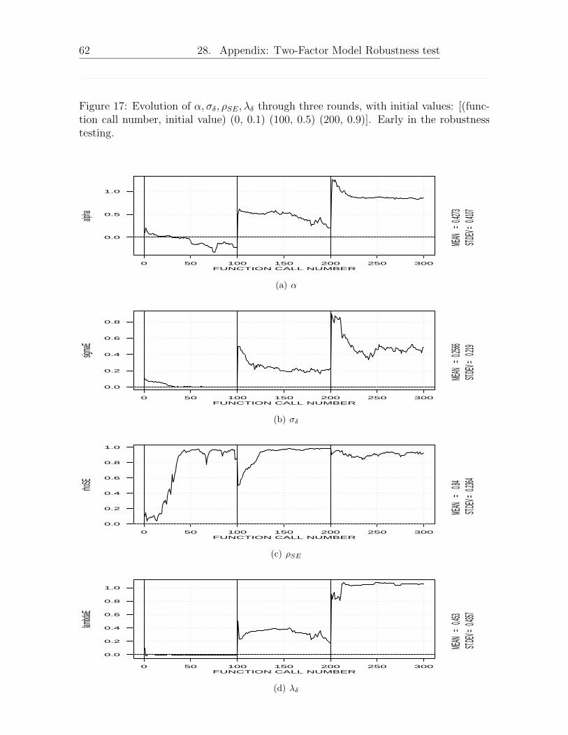
Kappa, alpha, sigmaE and lambda are clearly dependent on their initial values as
they do not converge to the same level in the three different rounds. Rho shows strong
evidence of convergence to roughly the same high level, 0.95. Mu and sigmaS appears
to converge. The initial high sigmaS is likely a result of the initial low rho.
The benefit of taking a round rather than a single function call is clear from the
first round — the parameters need time to settle. Seeing a rapid convergence, followed
by a stable evolution increases my confidence in the estimates.
61 28. Appendix: Two-Factor Model Robustness test
Figure 16: Evolution of µ, σs, κ through three rounds, with initial values: [(function callnumber, initial value) (0, 0.1) (100, 0.5) (200, 0.9)]. Early in the robustness testing.
0 50 100 150 200 250 300
−4
−2
0
2
4
6
8
FUNCTION CALL NUMBER
mu
MEAN
=
0.2089
ST.DEV
=
0.9433
(a) µ
0 50 100 150 200 250 300
0.5
1.0
1.5
2.0
2.5
FUNCTION CALL NUMBER
sigmaS
MEAN
=
0.4305
ST.DEV
=
0.3554
(b) σs
0 50 100 150 200 250 300
0.0
0.2
0.4
0.6
0.8
1.0
1.2
FUNCTION CALL NUMBER
kappaE
MEAN
=
0.6618
ST.DEV
=
0.4829
(c) κ
62 28. Appendix: Two-Factor Model Robustness test
Figure 17: Evolution of α, σδ, ρSE, λδ through three rounds, with initial values: [(func-tion call number, initial value) (0, 0.1) (100, 0.5) (200, 0.9)]. Early in the robustnesstesting.
0 50 100 150 200 250 300
0.0
0.5
1.0
FUNCTION CALL NUMBER
alpha
MEAN
=
0.4273
ST.DEV
=
0.4107
(a) α
0 50 100 150 200 250 300
0.0
0.2
0.4
0.6
0.8
FUNCTION CALL NUMBER
sigmaE
MEAN
=
0.2566
ST.DEV
=
0.219
(b) σδ
0 50 100 150 200 250 300
0.0
0.2
0.4
0.6
0.8
1.0
FUNCTION CALL NUMBER
rhoSE
MEAN
=
0.84ST.D
EV =
0.23
64
(c) ρSE
0 50 100 150 200 250 300
0.0
0.2
0.4
0.6
0.8
1.0
FUNCTION CALL NUMBER
lambda
E
MEAN
=
0.453
ST.DEV
=
0.4357
(d) λδ
63 28. Appendix: Two-Factor Model Robustness test
Fixing some parameters and optimize others I continue doing rounds with dif-
ferent initial values and different parameters being fixed. The choices made here are
clearly discretionary. As an example, I show in Figure 18 four rounds where I first fix
sigmaS at 0.4 and then in the second round change the level rho is fixed at from 0.95 to
0.9. kappaE, sigmaE and lambdaE responds to this change by increasing. In the last
two rounds I fix rho at 0.95, and let sigmaS be free to vary and set the initial of sigmasS
both below and above the value it appears to converge to. The initial value was 1 for
200 to 300 and 0.001 for 300 to 400. Observe how sigmaS fail to reach the frequently
observed level around 0.4 in round four. A sigmaS value of 0.001 is not reasonable to
have in the model anyway. Another problem when trying different initial conditions
is the interaction between the parameter values. That kappaE and sigmaE interact is
clear from round 2 (horizontal axis at 100-200) in Figure 18. For example in another
instance (not graphed) kappa and sigmaE rose together, reaching kappa = 2.2× 10112
and sigmaE = 1.02× 1048.
Figure 18: Robustness testing. Here I fix sigmaS (σS) and vary rhoSE (ρSE). (Sameinformation in the plot as in Figure 16 and 17, but a compact version.)
0.0
1.0
mu
0.0
0.6
sigm
aS
040
80
kapp
aE
0.0
0.3
0.6
0 100 200 300 400
alph
a
Time
015
30
sigm
aE
0.0
0.4
0.8
rhoS
E
02
4
0 100 200 300 400
lam
bdaE
Time
ts(allRegisteredParameterValues)
64 28. Appendix: Two-Factor Model Robustness test
Let them vary with informed initial values After rounds with different parame-
ters being fixed, I again let all vary, and set each parameter with an initial value both
below and above the level it appears to converge to. In some rounds are high values
of one parameter associated with high values of another parameter, resulting in asym-
metric behaviour and extreme values when they take off upwards away from the level
they should converge to. Some of the history of such later rounds are shown in Figure
19 and 20. At this point, instead of throwing out the vectors with values outside the
limit, I set the values on the axes to reasonable values. Then it is also seen for which
sets the estimates are out of bounds.
Curiously, to see how robust the convergence is, I set the initial value of rhoSE to
0.001 and 0.999. I get a kappaE of 8× 1034, which is not desirable to put in the model.
A value of rhoSE equal to 0.001 is not reasonable, so whether the model converges or
not from such values is not important. I argue that it suffices if the model is locally
convergent, if all parameters take on reasonable values in the local optimum. I therefore
now set initial values equal to the boarder of reasonable values and see whether they
converge from there. These later rounds are inclueded in Figure 19 and 20.
65 28. Appendix: Two-Factor Model Robustness test
Figure 19: Evolution of µ, σs, κ later in the robustness testing.
0 500 1000 1500 2000 2500
0.0
0.5
1.0
1.5
2.0
FUNCTION CALL NUMBER
mu
(a) µ
0 500 1000 1500 2000 2500
0.0
0.5
1.0
1.5
2.0
FUNCTION CALL NUMBER
sigmaS
(b) σs
0 500 1000 1500 2000 2500
0
5
10
15
20
25
30
FUNCTION CALL NUMBER
kappaE
(c) κ
66 28. Appendix: Two-Factor Model Robustness test
Figure 20: Evolution of α, σδ, ρSE, λδ later in the robustness testing.
0 500 1000 1500 2000 2500
0.0
0.5
1.0
1.5
2.0
FUNCTION CALL NUMBER
alpha
(a) α
0 500 1000 1500 2000 2500
0
1
2
3
4
5
FUNCTION CALL NUMBER
sigmaE
(b) σδ
0 500 1000 1500 2000 2500
0.90
0.92
0.94
0.96
0.98
1.00
FUNCTION CALL NUMBER
rhoSE
(c) ρSE
0 500 1000 1500 2000 2500
0
2
4
6
8
10
FUNCTION CALL NUMBER
lambda
E
(d) λδ
67 28. Appendix: Two-Factor Model Robustness test
Filtering the sample To increase the sample of output vectors from the optimization
function, do I initiate many rounds with a variety of settings. I then filter all these
stored output vectors according to my discretionary limits. I want to keep track off the
output vector, vector by vector, because the parameters are estimated together as a set
in the optimization function. Hence, I throw out the whole vector even if only one of
the parameters ends up outside its limits. After this, I am left with a filtered list of
vectors, where some vectors contain parameters which were not optimized (allowed to
vary). These vectors are not thrown out of the filtered matrix because they contribute
to variation for the other parameters.
Correcting What I do is to compute the mean and variance of the parameters on a
‘corrected subset’ of the parameters. The corrected subset consist only of observations
where two observations in a row are not equal, to take out the values where they were
fixed. I do this to avoid a bias in the computation of the mean and variance. E.g., if
I have set σS to be 0.4, I do not want 100 observations of 0.4 to be included in the
computation of the mean of the optimized value of sigma.
Conclusion regarding robustness The results (numbers found) are semi-robust in
the sense that they showed some evidence of convergence.
68 29. Appendix: Kalman Filter
29 Appendix: Kalman Filter
Hamilton (1994) explains the Kalman filter. The spot price is unobservable, that is the
problem. If the futures prices reflect the spot price, but not in a clear mapping from
one of the prices into the spot price, the idea is to use several prices to reason on what
the current spot price is. The futures prices are therefore noisy reflections of the spot
price. To have a system in state space form is a way of describing a dynamic system.
You need the current state and description on how you move into the next state. When
this is defined the Kalman filter is a technique when there are noise in the data. It
updates the prediction on the next state by punishing measurements with high variance
and high uncertainty. The Kalman filter assumes that the futures prices are normally
distributed, and it works best on linear systems, so the log-prices are preferred in the
representation to do the optimization.
69 30. Appendix: Maximum Likelihood Estimation
30 Appendix: Maximum Likelihood Estimation
Define:
• Sample = A particular sequence of observations:∑N
i=1 ui.
• Argument = A specific parameter value
MLE in short
Find the arguments that maximize the likelihood of actually observing the sample.
How:
(i) For each ui, assume a probability density function pdf(ui) to represent the prob-
ability of observing that particular observation.
(ii) The probability of observing the sample is L ≡∏m
i=1 pdf(ui) if the observations
are independent.
(iii) Take the natural logarithm of the function L to work with sums rather than
products.
(iv) Find the arguments of L that maximize L :
(a) Analytically, take the derivative of lnL with respect to the parameters of
interest.
(b) Iteratively, try different arguments in the lnL function and see which argu-
ment that yields the highest value of the function.
MLE in more detail
• To associate a probability with an observation, assume a probability density func-
tion pdf(ui) for the observation. For example the White-Noise pdf:
pdf(u;µ = 0, v) ≡ 1√(2πv)
exp
[u2i
2v
]= a exp[bi]
a ≡ 1√2πv
, bi ≡−u2
i
2v
• The likelihood of observing ui is defined as the output of a probability density
function.
70 30. Appendix: Maximum Likelihood Estimation
ui
Prob(u)
pdf(u)
u
The probability of observing ui.
• The likelihood of observing the sequence u1, u2, . . . , um is the product of the prob-
abilities if they are independent, so the likelihood is represented by the product
of the pdfs. Define this product as the likelihood L. If the pdfs are equal, the
likelihood of observing the particular sequence observed in the data set can be
written compactly as
L =m∏i=1
a exp[bi]
• The idea behind MLE is to identify the arguments for the function L such that
we maximize the likelihood of observing the sample. So it translates into finding
the values of the parameters that maximize L.
• A convenient trick is to take the natural logarithm before computing the derivative
as it greatly simplifies the computation of the derivative. This transformation is
monotonic, so the argument maximizing L will maximize lnL.
• Deriving the log-likelihood in detail for this particular White-Noise pdf:
L =m∏i=1
aebi =amm∏i=1
ebi ,
ln
(am
m∏i=1
ebi
)=m ln a+ Σm
i=1bi ln e
=m ln a+ Σmi=1bi
=m ln
(1√2πv
)+ Σm
i=1
−u2i
2v
=m ln
(1√2πv
)− 1
2vΣmi=1u
2i
=−m ln((2πv)0.5)
)− 1
2vΣmi=1u
2i
=− m
2ln (2πv)− 1
2vΣmi=1u
2i
• Maximizing the log-likelihood:
71 30. Appendix: Maximum Likelihood Estimation
– Iteratively, a computer program records the output value of the log-likelihood
function given different arguments. In this case, v will be varied until the
algorithm finds the argument for v that maximizes the output value of the
log-likelihood function. This is an iterative procedure, and it is an alternative
to the analytical solution.
– Analytically, take the derivative with respect to the parameter of interest
and set it equal to zero. Solve for the parameter to get an expression for the
optimal argument. To find the analytical solution for v in this case,
∂ lnL
∂v= −m
2v+
1
2v2Σmi=1u
2i
Set the derivative equal to zero and solve for v
−m2v
+1
2v2Σmi=1u
2i = 0
v∗ =Σmi=1u
2i
m
This is the optimal argument for the variance, v, in order to describe the
sample, given the assumed White-Noise pdf.
– For a simple regression, ui is the residuals from the regression ui = yi− βxi.– For GARCH, v is a non-constant function of ui. For example, Enders (2010)
page 154, the model AR(1) ut = yt − βyt−1 with ARCH(1) vt = a0 + a1u2t−1
has associated log-likelihood
lnL = −(m− 1)
2ln(2π)− 1
2
m∑t=2
ln(a0 + a1u
2t−1
)− 1
2
m∑t=2
(yt − βyt−1)2
a0 + a1u2t−1
where you can substitute in (yt−1 − βxt−1)2 for u2t−1
lnL = −(m− 1)
2ln(2π)−1
2
m∑t=2
ln(a0 + a1(yt−1 − βxt−1)2
)−1
2
m∑t=2
(yt − βyt−1)2
a0 + a1(yt−1 − βxt−1)2
and then maximize with respect to a0, a1, β.
72 31. Appendix: Deriving the Risk-Adjusted Process
31 Appendix: Deriving the Risk-Adjusted Process
Compute the present value of a uncertain cash flow.
To compute the present value ct of a claim cT in the future that depends the stochastic
price Ft and time, a model is constructed. I assume that the market is complete such
that all states of the uncertain cash fclow can be replicated. In this model Results are
exploited to make the model internally consistent, i.e. free from arbitrage opportunities.
A discussion on martingales and measures can be found in Chapter 28, Hull (2015).
Setting up the model:
Define the economy:
St = Futures price.
Dt =∫ t
0Ssδsds Accumulated convenience yield. δs = δ(s) a function of time only.
It is the money ‘saved’ because the futures cash flow is in the future.
At = ert A risk-free asset earning the constant risk-free rate r continuously.
ct = f(t, cT (ST )) Value of a claim as a function of time and its value at T .
cT = g(T, ST ) A cash flow at time T depending on ST .
Define gains in the economy:
G(1)t = St +Dt
G(2)t = At
G(3)t = ct
Discount by a numeraire security. Before presenting result i), discounting by a
numeraire security must be introduced. It means to denominate a security in terms of
another security, e.g. St/At. Here At is the numeraire security. Requirements for the
numeraire security are,
(i) that it must always have a strictly positive price to avoid division by zero.
(ii) The numeraire must not pay dividends if this is not accounted for.
If dividends are not incorporated, the identification of the drift correction would be
wrong, because it would fail to make the gains process a martingale. At is suitable to
be the numeraire security.
73 31. Appendix: Deriving the Risk-Adjusted Process
Define the discounted economy with At as the numeraire:
SAt ≡ St/AtDAt ≡
∫ t0
(δsSs)/Asds
AAt ≡ At/AtcAt ≡ ct/AtcAT ≡ cT/AT
Define discounted gains:
GA(1)t = SAt +DA
t
GA(2)t = AAt
GA(3)t = cAt
Specify the processes:
dSt = µ(t,Dt, St) dt+ γdWt , the drift µ(t,Dt, St) is specified generally.
dDt = δtSt dt
dAt = rAt dt
dct = df(t, cT (ST ))
dGA(1)t = d(SAt +DA
t )
dGA(2)t = dAAt
dGA(3)t = dcAt
Definition [1] The probability measure Q is equivalent relative to probability mea-
sure P, if all events E assigned zero probability with measure P, also are assigned zero
probability with measure Q. I.e.
Q(E) = 0 iff P (E) = 0
.
Definition [2] A random variable is a martingale if the expected value at time t, of
its future state in time T, for all T ≥ t, is equal to the state at time t. I.e.
Et{Xs} = Xt, ∀ s ≥ t
. The drift of a process must be zero for the process to be a martingale.
74 31. Appendix: Deriving the Risk-Adjusted Process
Definition [3] Using Definition [2] and [3] to define thatQ is an equivalent martingale
measure relative to P if (D1) and (D2) holds,
Q(E) = 0 iff P (E) = 0 (D1),
G∗(n)t = EQt {G∗(n)
s } , ∀ s ≥ t (D2).
Result [1] There are no arbitrage opportunities in the defined economy if and only if
there exists an equivalent martingale measure such that all discounted gains processes
are martingales.
Result [2] When we change from P to Q the standard Wiener process Wt relative to
P , will typically not be a standard Wiener process under Q. Girsanov’s theorem shows
that for arbitrary, but given λt the process dW λt = dWt + λdt is a standard Wiener
process under some probability measure M . When M = Q, M is the EMM. The
expected return changes, but the volatility remains the same when we move between
F and Q.
Exploiting Result [1] All discounted gains must be martingales to avoid arbitrage:
GA(1)t = SAt +DA
t = EQt {SAT +DAT }
GA(2)t = AAt = EQt {AAT } = EQt {1}
GA(3)t = cAt = EQt {cAT }
Under the probability measure Q, GA(2)t is a martingale by construction. G
A(1)t is the
restriction,, it is where Q is identified. Then, this Q is imposed on GA(3)t such that G
A(3)t
is a martingale by construction as well. Solve for ct (under Q) to obtain the price of
the security ct. The price ct is the price in both P and Q worlds, or else it would not be
useful. Because of the discounting with a particular numeraire security, the probability
measure found is also a particular one — it corresponds to the particular numeraire.
75 31. Appendix: Deriving the Risk-Adjusted Process
Make all discounted gains process martingales:
dGA(3)t = will be by construction
dGA(2)t = d(AAt ) = 0
dGA(1)t = d(SAt +DA
t )
=
(1
AtdSt + 0
1
2dS2
t −StA2t
dAt +StA3t
1
2���>
0dA2
t − 1
At
1
2���
��:0dAtdSt
)+
(δ(t)StAt
dt
)=
1
AtdSt −
StA2t
dAt +δ(t)StAt
dt
=1
At[µ(t,Dt, St) dt+ γdWt]−
StA2t
[rAtdt] +δ(t)StAt
dt
=1
At[µ(t,Dt, St)− St (r − δ(t))] dt+ γdWt
dGA(1)t is not a martingale because the drift 1
At[µ(t,Dt, St)− St (r − δ(t))] dt is not zero.
Now use Girsanov’s theorem to make it a martingale under another probability measure.
Insert dW λt − λtdt, for dWt.
dGA(1)t =
1
At[µ(t,Dt, St)− St (r − δ(t))] dt+ γ
[dW λ
t − λtdt]
=1
At[µ(t,Dt, St)− St (r − δ(t))− γλt] dt+ γdW λ
t
Can set λt as you want, so choose it so the drift is zero.
λt =µ(t,Dt, St)− St (r − δ(t))
γ
76 31. Appendix: Deriving the Risk-Adjusted Process
For this choice of lambda, is dGA(1)t a martingale. Apply the measure found to risk
adjust dSt. Denote St with λ to emphasise that it is under the risk-neutral measure.
dSt = µ(t,Dt, St) dt+ γdWt
dSλt = µ(t,Dt, St) dt+ γ[dW λ
t − λtdt]
= (µ(t,Dt, St)− γλt) dt+ γdW λt
dSλt =
(µ(t,Dt, St)− γ
[µ(t,Dt, St)− Sλt (r − δ(t))
γ
])dt+ γdW λ
t
dSλt = Sλt (r − δ(t)) dt+ γdW λt (50)
The particular drift µ(t,Dt, St) disappears. The volatility is the same in both worlds.
Here the convenience yield δ(t) is allowed to vary through time deterministically. This
is useful if one wants to incorporate (possibly through an Euler scheme) an opinion on
the convenience yield in the pricing model.
Specify the function CT = g(T, ST ) as desired. The present value of the derivative
in this model is
ct = AtEQt{CTAT
}= e−r(T−t)EQt {CT} . (51)
AT is deterministic, so it goes out of the expectation.
ct is found by using the Q measure in the expectation to find ct — that is, to use the
dynamics, (50), developed under the Q measure in the computation of the expectation.
If it is difficult to obtain an analytical solution is it possible to take the expectation by
simulation of the discrete version of the differential equation developed under Q. The
time step could have a role, as discussed in Appendix: The (Possible) Role of ∆t.
77 31. Appendix: Deriving the Risk-Adjusted Process
Constant convenience yield For a constant δt = δ the solution to (50) is
SλT = Sλt e(r−δ)(T−t) + γeT (r−δ)
∫ T
t
e−s(r−δ)dW λs (52)
EQt {SλT} = Sλt e(r−δ)(T−t) (53)
Var(SλT ) = γ2e2T (r−δ)∫ T
t
e−2s(r−δ)ds =γ2
2(r − δ)(e2(r−δ)(T−t) − 1
)(54)
Convenient to have the following expressions for a call option computation
EQt {SλT} ≡ m
Var(SλT ) ≡ v2
SλTdist.= m+ v η , η ∼ N(0, 1)
1{ST≥K} = 1 if ST ≥ K
1{ST≥K} = 0 if ST < K
E{1{ST≥K}ST} =
∫ ∞−∞
1{m+v η≥K}(m+ v η)1√2πe−
12η2dη
= m
∫ ∞K−m
v
1√2πe−
12η2dη +
∫ ∞K−m
v
v η1√2πe−
12η2dη
= mN
(−(K −mv
))+
v√2π
∫ ∞K−m
v
ηe−12η2dη
= mN
(m−Kv
)+
v√2π
[−e−
12η2]∞
K−mv
= mN
(m−Kv
)+
v√2πe−
12(K−m
v )2
(55)
E{1{ST≥K}} =
∫ ∞−∞
1{m+v η≥K}1√2πe−
12η2dη
= N
(m−Kv
)(56)
78 31. Appendix: Deriving the Risk-Adjusted Process
A call option:
ct = e−r(T−t)EQt {max(ST −K, 0)}
ct = e−r(T−t)EQt{
1{ST≥K}(ST −K)}
ct = e−r(T−t)(EQt{
1{ST≥K}ST}−KEQt
{1{ST≥K}
})ct = e−r(T−t)
(mN
(m−Kv
)+
v√2πe−
12(K−m
v )2
−KN(m−Kv
))ct = e−r(T−t)
(v√2πe−
12(K−m
v )2
+[Sλt e
(r−δ)(T−t) −K]N
(m−Kv
))(57)
79 31. Appendix: Deriving the Risk-Adjusted Process
Futures contract: The present value of a futures contract maturing in T , entered
into in the past, to buy steel for K will have the present value ct,T