Modeling Tools for Drilling, Reservoir Navigation, and Formation Evaluation

Sushant DUTTAFei LE

Alexandre BESPALOVArcady REIDERMAN

Michael RABINOVICHDrilling & Evaluation Research, Baker Hughes, 2001 Rankin Road,

Houston, TX 77073, USA

ABSTRACT

The oil and gas industry routinely uses borehole tools for measur-ing or logging rock and fluid properties of geologic formations tolocate hydrocarbons and maximize their production. Pore fluidsin formations of interest are usually hydrocarbons or water. Re-sistivity logging is based on the fact that oil and gas have a sub-stantially higher resistivity than water. The first resistivity logwas acquired in 1927, and resistivity logging is still the foremostmeasurement used for drilling and evaluation. However, the ac-quisition and interpretation of resistivity logging data has grownin complexity over the years.

Resistivity logging tools operate in a wide range of frequencies(from DC to GHz) and encounter extremely high (several or-ders of magnitude) conductivity contrast between the metal man-drel of the tool and the geologic formation. Typical challengesinclude arbitrary angles of tool inclination, full tensor electricand magnetic field measurements, and interpretation of compli-cated anisotropic formation properties. These challenges com-bine to form some of the most intractable computational elec-tromagnetic problems in the world. Reliable, fast, and con-venient numerical modeling of logging tool responses is crit-ical for tool design, sensor optimization, virtual prototyping,and log data inversion. This spectrum of applications necessi-tates both depth and breadth of modeling software—from blazingfast one-dimensional (1-D) modeling codes to advanced three-dimensional (3-D) modeling software, and from in-house devel-oped codes to commercial modeling packages.

In this paper, with the help of several examples, we demonstrateour approach for using different modeling software to addressdifferent drilling and evaluation applications. In one example,fast 1-D modeling provides proactive geosteering informationfrom a deep-reading azimuthal propagation resistivity measure-ment. In the second example, a 3-D model with multiple verticalresistive fractures successfully explains the unusual curve separa-tions of an array laterolog tool in a shale-gas formation. The thirdexample uses two-dimensional (2-D) and 3-D modeling to provethe efficacy of a new borehole technology for reservoir monitor-ing.

Keywords: Modeling, oil and gas, reservoir navigation, forma-tion evaluation, array laterolog, reservoir monitoring, transientelectromagnetics

1. INTRODUCTION

Borehole tools are routinely used in the oil and gas industry tomeasure rock and fluid properties in and around the wellbore.

This branch of the oil and gas industry is called well logging.Well logging tools that perform measurements while the wellis being drilled are called logging-while-drilling (LWD) tools,while those that perform measurements after the well has beendrilled are called wireline tools. The foremost application ofLWD tools is reservoir navigation, which is the matching of geo-logical and other physical models to drill along and through bedboundaries to precisely place wells. The primary application ofwireline tools, as well as another important application of LWDtools, is formation evaluation, which is the process of interpretinga combination of measurements taken inside the wellbore to de-tect and quantify oil and gas reserves and production potential inthe rock adjacent to the well. The data from these measurementsare usually organized and interpreted by depth and representedon a graph called a log.

Borehole logging tools can be categorized based on the toolphysics and application as electrical resistivity tools, nucleartools, nuclear magnetic resonance (NMR) tools, and acoustictools. This paper deals with resistivity tools. The first electricalresistivity log was acquired in 1927, and today resistivity remainsthe most important rock property to the oil and gas industry. Porefluids in geological formations of interest are usually hydrocar-bons or water. Oil and gas have a substantially higher electricalresistivity compared to water. Hence the resistivity of a geolog-ical formation, taken in the right context, is a clear indicator ofthe hydrocarbon content as well as the lithostratigraphy of theformation.

Reliable, fast, and convenient numerical modeling of tool re-sponses is critical for tool design, sensor optimization, virtualprototyping, and log data inversion. Over the years, the acqui-sition and interpretation of resistivity data has grown in com-plexity and it has become increasingly difficult to develop anduse a single modeling package for all applications. This paperdescribes our modeling philosophy for different resistivity toolsand applications. The rest of this paper is organized as follows.Section 2 describes the physics of different types of resistivitytools and general modeling principles for resistivity tools. Sec-tion 3 presents three case studies that belong to different appli-cations and follow different modeling methods. In the first ex-ample, fast one-dimensional (1-D) modeling provides proactivegeosteering information from a deep-reading azimuthal propaga-tion resistivity measurement. In the second example, a three-dimensional (3-D) model with multiple vertical resistive frac-tures successfully explains the unusual curve separations of anarray laterolog tool in a shale-gas formation. The third exam-ple uses two-dimensional (2-D) and 3-D modeling to prove theefficacy of a new borehole technology for reservoir monitoring.

SYSTEMICS, CYBERNETICS AND INFORMATICS VOLUME 10 - NUMBER 3 - YEAR 2012 81ISSN: 1690-4524

Section 4 discusses our modeling philosophy and concludes thepaper.

2. PHYSICS OF RESISTIVITY TOOLS

Before discussing tool physics, it is pertinent to introduce typ-ical scenarios in which resistivity tools operate and which af-fect tool physics and measurements. The wellbore is filled withdrilling fluid (also called drilling mud) while the well is beingdrilled. The drilling fluid could be water-based (conductive) oroil-based (resistive). With time, the drilling fluid typically in-vades the formation close to the wellbore, especially if the for-mation is permeable, and leaves a layer of solid residue (calledmud cake) on the borehole wall. This tends to affect resistivitymeasurements, especially in the case of wireline logging which isusually performed hours after the well is drilled. For some resis-tivity tools, the eccentricity of the tool in the wellbore affects themeasurements. Nearby bed boundaries with resistivity contrastscan make the interpretation of resistivity data problematic. Sim-ilarly, anisotropy in the formation can lead to misleading mea-surements.

In general, all resistivity tools generate electromagnetic fieldswhich obey Maxwells equations:

∇×H = Jf +∂D

∂t(1)

∇×E = −∂B∂t

(2)

∇ ·D = ρf (3)

∇ ·B = 0 (4)

along with the following constitutive relations for anisotropicmedia:

D = ε ·E (5)

B = µ ·H (6)

J = σ ·E (7)

and interface conditions:

n× (H1 −H2) = JS (8)

n× (E1 −E2) = 0 (9)

where H is the magnetic field intensity, E is the electric fieldintensity, D is the electric flux density (displacement), B is themagnetic flux density, Jf is the free electric current density, ρfis the free electric charge density, ε is the electric permittivity, µis the magnetic permeability, σ is the electric conductivity, JS isthe surface current density on the interface, n is the normal vectorto the interface. J is the bound current density and is given byJ = Jf − Je, where Je is the external current density.

GalvanicGalvanic tools use a measurement (active) electrode to directlyinject current into the formation. The injected current flows backto the tool via a return (passive) electrode. Galvanic tools usuallyoperate on DC or low-frequency (< 10 kHz) AC. Fig. 1(a) showsa schematic diagram of a typical galvanic tool. Galvanic tools ina vertical borehole respond to resistances across horizontal bedboundaries in series. Hence they are more suited to water-basedmuds because the current can flow through the conductive mud

into the formation easily. Under the DC approximation, the time-variation of electromagnetic quantities is negligible and Eqs. (1)and (2) reduce to

∇×H = Je + σ ·E (10)

∇×E = 0 (11)

InductionInduction tools use a transmitter coil to generate a time-varying(usually time-harmonic with angular frequency ω) magneticfield. This magnetic field induces a time-varying electric field(and hence eddy currents) in the formation. The secondary mag-netic field generated by the formation eddy currents is propor-tional to formation conductivity and is measured by a receivercoil. Induction tools necessarily operate on AC and are well-suited to oil-based muds. Fig. 1(b) shows a schematic diagram ofa typical induction tool. An induction tool in a vertical boreholeresponds to resistances across horizontal bed boundaries in par-allel. For the time-harmonic fields in the low-to-mid-frequencyrange (typically up to 400 kHz), we can assume stationary cur-rents at every instant. Then the displacement current is negligibleand Eqs. (1) and (2) reduce to

∇×H = Je + σ ·E (12)

∇×E = −j ωµ ·H (13)

where j =√−1.

PropagationPropagation tools form a special class of induction tools that op-erate on high frequencies (400 kHz–GHz range). In this rangeof frequencies, the displacement current may not be negligibleand there can be significant phase shift in the time-harmonic sig-nal measured at the receiver. In fact, as the operating frequencyincreases in this range, we obtain another special class of toolscalled dielectric tools. Their operating frequencies are so highthat displacement currents may dominate conduction currents,and these tools can measure permittivity as well as resistivity. Forpropagation resistivity tools, Eqs. (1) and (2) reduce to

∇×H = Je + σ ·E + j ω ε ·E (14)

∇×E = −j ωµ ·H (15)

TransientStrictly speaking, transient tools are also induction tools but theyare categorized separately because they are very different in the-ory and practice from the usual time-harmonic tools. In fact,transient tools are only used in surface geophysics and have neverbeen used in borehole applications. Their principle of operationis as follows: (1) the transmitter is energized with a constant DCexcitation until all transient effects expire; (2) the constant exci-tation is then abruptly cut off; (3) the abrupt cut-off is a broad-band excitation which induces eddy currents in the formation thatare proportional to the formation conductivity; (4) the inducededdy currents diffuse farther and become weaker over time; (5)the receiver measures the rate of change of secondary magneticfield of the formation eddy currents as a function of time. Hencetransient measurements are performed in the absence of primaryfields. Propagation effects are negligible in the time range of in-terest, and Eqs. (1) and (2) reduce to

∇×H = Je + σ ·E (16)

∇×E = −∂B∂t

(17)

SYSTEMICS, CYBERNETICS AND INFORMATICS VOLUME 10 - NUMBER 3 - YEAR 201282 ISSN: 1690-4524

Mandrel

Formation

Borehole Conductive

currents

Active

electrode(s)

Passive

electrode(s)

Insulation

(a) Galvanic tool

Mandrel

Formation

Transmitter coil

Receiver coil

Primary

magnetic

field

Induced

currents

Secondary

magnetic

field

Borehole

(b) Induction tool

Fig. 1: Schematic diagrams of two typical kinds of resistivitytools

As seen above, resistivity tools operate in a wide range of fre-quencies (from DC to GHz). They obey different tool physicsand impose different requirements on modeling programs. Mod-eling requirements are also subject to applications such as proof-of-concept studies, tool design and sensor optimization, and datainversion. Other challenges include extremely high (several or-ders of magnitude) conductivity contrast between the metal man-drel of the tool and the geologic formation, arbitrary anglesof tool inclination, full tensor electric and magnetic field mea-surements, and interpretation of complicated anisotropic forma-tion properties. These challenges combine to form some of themost intractable computational electromagnetic problems in theworld. We rely on a suite of modeling programs to accom-plish reliable, fast, and convenient numerical modeling of toolresponses on a case-by-case basis. The numerical methods couldbe semi-analytical, finite-difference method (FDM), or finite-element method (FEM). In the next section, we discuss three dif-ferent applications of numerical modeling of borehole resistivitytools.

3. CASE STUDIES

GeosteeringReservoir navigation (i.e., geosteering) while drilling is a veryimportant application area for resistivity tools. Geosteering isused to land wells at predetermined locations in a reservoir andto stay within specific regions of the reservoir to optimize thepotential production of hydrocarbons. Deep-reading azimuthalpropagation resistivity tools provide proactive geosteering infor-mation by indicating approaching boundaries before the well-bore actually penetrates them, thus enabling precise control of

Fig. 2: Simulated deep resistivity image for a straight-line welltrajectory entering and leaving a reservoir at 70 relative dip

the wellbore trajectory in real time [1]. Qualitative recognitionof an approaching boundary and the quantitative prediction of thedistance to the boundary (D2B) are both invaluable if they can beaccomplished in real time.

For deep-reading propagation resistivity tools, the borehole andthe volume of formation adjacent to the borehole usually do notaffect the signals. Under these conditions, it is usually feasi-ble to represent the formation and the reservoir as a layered 1-Dstructure with resistivity contrasts between different layers. Fastresistivity forward models are then used for pre-job planning aswell as for real-time D2B inversion and geosteering along a de-sired well trajectory. As the formation model is relatively simple(1-D) and solution speed is imperative, the forward models con-sider the transmitter and receiver as point magnetic dipoles andfast semi-analytical software is used to solve forward models iter-atively for real-time inversion. The metal mandrel is not implicitin the forward models, but its effect is empirically incorporatedinto the forward model results. Fig. 2 shows the deep resistivityimage this software generated for a straight-line wellbore with70 relative dip (angle made by the wellbore trajectory with thenormal to the bed boundary). The top panel shows the wellboretrajectory and the 1-D layered formation model. The y-axis rep-resents the true vertical depth (TVD) of the tool, while the x-axis represents the measured depth of the tool (the distance mea-sured along the trajectory). The gray shaded layer is the reservoirwhich is ten times as resistive as the formation above and belowit. The bottom panel is the deep resistivity image generated usingthe simulated coaxial and azimuthal propagation resistivity sig-nals for 400 kHz frequency. The y-axis represents the boreholeazimuth (T: top, B: bottom, L: left, R: right). It is clear that thepropagation resistivity tool ‘sees’ the approaching bed boundaryas much as 10 m (in terms of measured depth) away. In addition,the tool predicts whether the bed boundary is approaching thewellbore trajectory from above or below.

The information contained in deep resistivity images can helpdrillers to geosteer the well to their advantage [2]. Fig. 3 showsa realistic reservoir navigation case in which the well enters thereservoir and continues to be drilled at 70 relative dip until itreaches close to the bottom of the reservoir (as indicated by thedeep resistivity image). After obtaining this good estimate ofthe thickness of the reservoir, the wellbore is steered up until itreaches close to the roof of the reservoir. From this point on, thetrajectory is maintained at a fixed distance below the roof of thereservoir.

SYSTEMICS, CYBERNETICS AND INFORMATICS VOLUME 10 - NUMBER 3 - YEAR 2012 83ISSN: 1690-4524

Fig. 3: Simulated deep resistivity image for a realistic geosteer-ing scenario where the well is landed in the reservoir at 70 rela-tive dip and then steered to stay within the reservoir close to theroof

Apart from actual signal inversion to estimate the distance to bedboundaries, these modeled deep resistivity images are also com-pared to deep resistivity images generated at the rig in real timeto make geosteering decisions and to improve the model of thereservoir.

Array Laterolog Tool in Shale-Gas FormationAn array laterolog is a DC galvanic tool with multiple electrodespacings. The electrodes are activated in different configura-tions (called modes) which govern how deep the current pene-trates into the formation, so that the tool yields multiple resistiv-ity curves for different distances from the tool [3]. The distancebetween the tool and the region of formation being investigatedis called depth of investigation (DOI). The tool measures appar-ent resistivity, which is the resistivity of a hypothetical homoge-neous formation that would yield the same voltage-current rela-tionship as the actual formation under investigation. In this sec-tion we describe a case study involving unusual array laterologsignals measured in numerous wells in the Bossier formation ofthe Haynesville shale region in Louisiana. When multiple resis-tivity curves obtained from galvanic or induction instruments donot coincide, this can often be attributed to the invasion of drillingfluids into the formation. The resistivity curves measured by thearray laterolog in the above region also showed considerable sep-aration, as shown in the boxed part of the resistivity log in Fig. 4[4]. However, the Bossier formation has extremely low perme-ability, so that drilling fluid invasion cannot explain the curveseparations. To explain the curve separations, a 3-D model witha set of parallel, vertical, gas-filled resistive fractures/thin lami-nations was proposed, as shown in Fig. 5.

A 3-D FEM software package is used to obtain the static solu-tion for different electrode modes (and their corresponding DOI).Fig. 6 shows these results for different fracture and invasioncases. A single fracture across the borehole is called a drilling-induced fracture. The overlap of the red and brown curves indi-cates that a single drilling-induced fracture has no effect on thearray laterolog response. When multiple parallel resistive frac-tures are introduced into the model, we see that the array lat-erolog modes with higher DOI show significant increase in themeasured apparent resistivity, which explains the curve separa-tions in Fig. 4.

To understand the reason for the curve separations in the array

Fig. 4: Array laterolog resistivity curves logged in the upper andmiddle Bossier formation. Note the resistivity curve separationsin the middle Bossier log response (boxed in red).

laterolog responses, the conductive current density distributionin the vertical y-z plane is plotted for the shallowest mode (DOI= 22.86 cm) and the deepest mode (DOI = 93.98 cm), as shownin Fig. 7. The activated electrodes are shown in red, while thereturn electrodes are shown in blue. The current distribution inthe shallowest mode is not significantly affected by the fracturesbecause the DOI of this mode is smaller than the distance ofthe tool from the nearest fracture. The deepest mode, in con-trast, has many more electrodes activated, and the DOI is threetimes the inter-fracture spacing. Clearly, fractures obstruct anddeform the current distribution in the deepest mode. As the DOIincreases, the conduction current ‘sees’ an increasing number ofresistive fractures, thus increasing the measured apparent resis-

6.35 mm

31.12 cm

25.08 cm

Borehole 0.25 .m

5 .m

Fracture

10 k .m

30.48 cm

Invasion 𝜙

Ω

Ω Ω

𝑦

𝑥

Fig. 5: 3-D model with vertical resistive fractures proposed toexplain resistivity curve separations

SYSTEMICS, CYBERNETICS AND INFORMATICS VOLUME 10 - NUMBER 3 - YEAR 201284 ISSN: 1690-4524

20 30 40 50 60 70 80 90 1002

4

6

8

10

12

14

16

18

Depth of investigation, cm

App

aren

t res

istiv

ity, Ω

⋅ m

20 30 40 50 60 70 80 90 1002

4

6

8

10

12

14

16

18

Depth of investigation, cm

App

aren

t res

istiv

ity, Ω

⋅ m

No fracture, no invasionDrilling−induced fracture, no invasionDrilling−induced fracture, with invasionParallel fractures, no invasionParallel fractures, with invasion

Fig. 6: Simulated array laterolog apparent resistivity as a func-tion of DOI for different fracture and invasion cases

(a) Shallowest mode (DOI = 22.86 cm)

(b) Deepest mode (DOI = 93.98 cm)

Fig. 7: Currrent density maps in y-z plane for array laterolog information with vertical resistive fractures

tivity.

Other simulations have indicated that, as the fracture width andinter-fracture spacing decrease, the apparent resistivity increasesfor each mode. In the limit of the fracture width approach-ing zero, the proposed fracture model resembles a uniaxiallyanisotropic formation with the same electrical properties in x andz directions, but different in y direction.

Reservoir MonitoringOil fields are very dynamic over their lifetime. As the amount ofoil in a producing oil field is depleted, various techniques are im-plemented to exploit the oil field to the maximum and keep theproduction process economical. Enhanced oil recovery (EOR)processes such as waterflooding, steam flooding, and chemicalflooding are extensively used all over the world to produce oilfrom mature oil fields. These processes involve the use of an in-jector well to inject water, steam, or water-based chemicals intothe reservoir. The injected fluids help maintain the reservoir pres-sure and drive oil to the producer well. EOR processes causekey changes in reservoir fluid composition over time. Reser-

R

T

50 – 300 m

50 m Waterflood

front

Shale

2 .m

Shale

Producer

well

Oil

40 .m 0.5 .m

Azimuthally

symmetric

Ω

Ω Ω

𝑧 𝑟

Fig. 8: Proof-of-concept model for reservoir monitoring usingTEM borehole technology

voir monitoring—accurately mapping the fluid distribution andfluid dynamics at the reservoir scale—is critical for obtaining thebest results from EOR processes. Reservoir monitoring is a rel-atively new application area for resistivity tools. Over the lasttwenty years, crosswell tomographic borehole electromagnetictechniques have been used for reservoir monitoring [5].

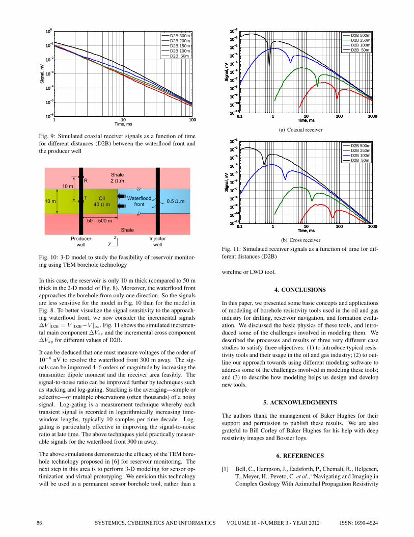
Very recently, a novel transient electromagnetic (TEM) boreholetechnology was applied to reservoir monitoring [6]. A 2-D FEMsoftware was used to conduct transient simulations for initialproof-of-concept studies. Later, 3-D FEM software was usedfor feasibility studies. Fig. 8 shows the axisymmetric proof-of-concept model. It assumes a 50 m-thick oil reservoir withconductive shale above and below. The waterflood front is az-imuthally symmetric around the borehole and advances towardsthe borehole with time. This is a simplification of the case wherethe producer well is surrounded by many equidistant and identi-cal injector wells. The transmitter and receiver coils are placedcoaxially in the producer well and point along the wellbore axis.The producer well casing is assumed to be non-conductive, atleast in the region close to the transmitter and receiver, and henceneglected.

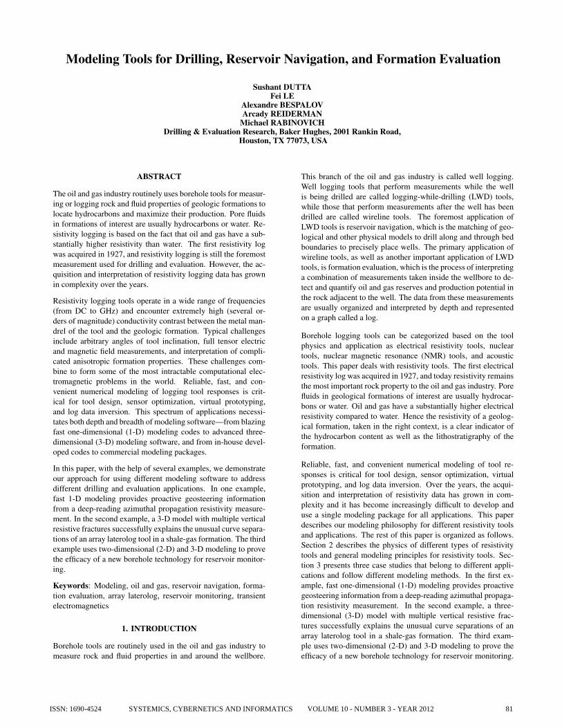
The distance between the producer wellbore and the waterfloodfront is denoted by D2B. Fig. 9 shows the simulated transientcoaxial receiver signals for different values of D2B. The signalsare calculated for unit transmitter dipole moment and unit re-ceiver area. TEM signals are characterized by very large dynamicrange, typically one to five decades of amplitude per two decadesof time. It is clear from the simulations that this method is sen-sitive to a radial waterflood front 300 m away. After proving theconcept of a borehole TEM reservoir monitoring system using2-D axisymmetric simulations, a 3-D model was constructed forthe feasibility study [6], as shown in Fig. 10. This is a more real-istic model which addresses the worst-case reservoir monitoringscenario. It assumes a 10 m-thick oil reservoir with conductiveshale above and below. There is only one injector well a largedistance away on the right, so that the waterflood front can beassumed to be planar, and it advances towards the producer wellwith time. Again, the producer well casing is assumed to be non-conductive. Triaxial transmitter and receiver coils are placed inthe producer well and all nine components of the voltage tensorcan be calculated. Dutta et al. [6] have shown that measure-ment of the three diagonal elements of the voltage tensor (Vxx,Vyy , and Vzz) is the minimum requirement for determining theazimuthal location of the waterflood front.

SYSTEMICS, CYBERNETICS AND INFORMATICS VOLUME 10 - NUMBER 3 - YEAR 2012 85ISSN: 1690-4524

1 10 10010

−6

10−5

10−4

10−3

10−2

10−1

100

Time, ms

Sig

nal,

nV

D2B 300mD2B 200mD2B 150mD2B 100mD2B 50m

1 10 10010

−6

10−5

10−4

10−3

10−2

10−1

100

Time, ms

Sig

nal,

nV

Fig. 9: Simulated coaxial receiver signals as a function of timefor different distances (D2B) between the waterflood front andthe producer well

R

T

50 – 500 m

10 m Waterflood

front

Shale

2 .m

Shale

Producer

well

Oil

40 .m 0.5 .m

10 m

Injector

well

Ω

Ω Ω

𝑧 𝑦

Fig. 10: 3-D model to study the feasibility of reservoir monitor-ing using TEM borehole technology

In this case, the reservoir is only 10 m thick (compared to 50 mthick in the 2-D model of Fig. 8). Moreover, the waterflood frontapproaches the borehole from only one direction. So the signalsare less sensitive for the model in Fig. 10 than for the model inFig. 8. To better visualize the signal sensitivity to the approach-ing waterflood front, we now consider the incremental signals∆V |D2B = V |D2B−V |∞. Fig. 11 shows the simulated incremen-tal main component ∆Vzz and the incremental cross component∆Vzy for different values of D2B.

It can be deduced that one must measure voltages of the order of10−6 nV to resolve the waterflood front 300 m away. The sig-nals can be improved 4–6 orders of magnitude by increasing thetransmitter dipole moment and the receiver area feasibly. Thesignal-to-noise ratio can be improved further by techniques suchas stacking and log-gating. Stacking is the averaging—simple orselective—of multiple observations (often thousands) of a noisysignal. Log-gating is a measurement technique whereby eachtransient signal is recorded in logarithmically increasing time-window lengths, typically 10 samples per time decade. Log-gating is particularly effective in improving the signal-to-noiseratio at late time. The above techniques yield practically measur-able signals for the waterflood front 300 m away.

The above simulations demonstrate the efficacy of the TEM bore-hole technology proposed in [6] for reservoir monitoring. Thenext step in this area is to perform 3-D modeling for sensor op-timization and virtual prototyping. We envision this technologywill be used in a permanent sensor borehole tool, rather than a

0.1 1 10 100 100010

−11

10−10

10−9

10−8

10−7

10−6

10−5

10−4

10−3

10−2

10−1

Time, ms

Sig

nal,

nV

0.1 1 10 100 100010

−11

10−10

10−9

10−8

10−7

10−6

10−5

10−4

10−3

10−2

10−1

Time, ms

Sig

nal,

nV

0.1 1 10 100 100010

−11

10−10

10−9

10−8

10−7

10−6

10−5

10−4

10−3

10−2

10−1

Time, ms

Sig

nal,

nV

0.1 1 10 100 100010

−11

10−10

10−9

10−8

10−7

10−6

10−5

10−4

10−3

10−2

10−1

Time, ms

Sig

nal,

nV

0.1 1 10 100 100010

−11

10−10

10−9

10−8

10−7

10−6

10−5

10−4

10−3

10−2

10−1

Time, ms

Sig

nal,

nV

D2B 500mD2B 250mD2B 100mD2B 50m

(a) Coaxial receiver

0.1 1 10 100 100010

−11

10−10

10−9

10−8

10−7

10−6

10−5

10−4

10−3

10−2

10−1

Time, msS

igna

l, nV

0.1 1 10 100 100010

−11

10−10

10−9

10−8

10−7

10−6

10−5

10−4

10−3

10−2

10−1

Time, msS

igna

l, nV

0.1 1 10 100 100010

−11

10−10

10−9

10−8

10−7

10−6

10−5

10−4

10−3

10−2

10−1

Time, msS

igna

l, nV

0.1 1 10 100 100010

−11

10−10

10−9

10−8

10−7

10−6

10−5

10−4

10−3

10−2

10−1

Time, msS

igna

l, nV

0.1 1 10 100 100010

−11

10−10

10−9

10−8

10−7

10−6

10−5

10−4

10−3

10−2

10−1

Time, msS

igna

l, nV

D2B 500mD2B 250mD2B 100mD2B 50m

(b) Cross receiver

Fig. 11: Simulated receiver signals as a function of time for dif-ferent distances (D2B)

wireline or LWD tool.

4. CONCLUSIONS

In this paper, we presented some basic concepts and applicationsof modeling of borehole resistivity tools used in the oil and gasindustry for drilling, reservoir navigation, and formation evalu-ation. We discussed the basic physics of these tools, and intro-duced some of the challenges involved in modeling them. Wedescribed the processes and results of three very different casestudies to satisfy three objectives: (1) to introduce typical resis-tivity tools and their usage in the oil and gas industry; (2) to out-line our approach towards using different modeling software toaddress some of the challenges involved in modeling these tools;and (3) to describe how modeling helps us design and developnew tools.

5. ACKNOWLEDGMENTS

The authors thank the management of Baker Hughes for theirsupport and permission to publish these results. We are alsograteful to Bill Corley of Baker Hughes for his help with deepresistivity images and Bossier logs.

6. REFERENCES

[1] Bell, C., Hampson, J., Eadsforth, P., Chemali, R., Helgesen,T., Meyer, H., Peveto, C. et al., “Navigating and Imaging inComplex Geology With Azimuthal Propagation Resistivity

SYSTEMICS, CYBERNETICS AND INFORMATICS VOLUME 10 - NUMBER 3 - YEAR 201286 ISSN: 1690-4524

While Drilling”, Proc. of SPE Annual Technical Con-ference and Exhibition, San Antonio, Texas, USA, 24–27September 2006, Paper 102637.

[2] Kennedy, W.D., Corley, B., Painchaud, S., Nardi, G., andHart, E., “Geosteering Using Deep Resistivity Images fromAzimuthal and Multiple Propagation Resistivity”, Proc. ofSPWLA Annual Logging Symposium, The Woodlands,Texas, USA, 21–24 June 2009.

[3] Zhou, Z., Corley, B., Khokhar, R., Maurer, H.-M., and Ra-binovich, M., “A New Multi Laterolog Tool with AdaptiveBorehole Correction”, Proc. of SPE Annual TechnicalConference and Exhibition, Denver, Colorado, USA, 21–24 September 2008, Paper 114704.

[4] Corley, B., Garcia, A., Maurer, H., Rabinovich, M., Zhou,Z., Dubois, P., and Shaw, N. Jr., “Study of Unusual Re-sponses from Multiple Resistivity Tools in the Bossier For-mation of the Haynesville Shale Play”, Proc. of SPEAnnual Technical Conference and Exhibition, Florence,Italy, 19–22 September 2010, Paper 134494.

[5] Mieles, L., Darnet M., Popta, J.V., Singh, M., Wilt, M., andLevesque, C., “Experience with Crosswell Electromagnet-ics (EM) for Waterflood Management in Oman”, Proc. ofInternational Petroleum Technology Conference, Doha,Qatar, 7–9 December 2009.

[6] Dutta, S.M., Reiderman, A., Schoonover, L.G., and Rabi-novich, M.B., “New Transient Electromagnetic BoreholeSystem for Reservoir Monitoring”, presented at SPWLATopical Conference, Abu Dhabi, UAE, 14–17 March2011.

SYSTEMICS, CYBERNETICS AND INFORMATICS VOLUME 10 - NUMBER 3 - YEAR 2012 87ISSN: 1690-4524