Modeling Urban Land Use Change and Urban Sprawl:Calgary, Alberta, Canada

Heng Sun & Wayne Forsythe & Nigel Waters

Published online: 7 August 2007# Springer Science + Business Media, LLC 2007

Abstract This paper implements a land use classification for the City of Calgary,Alberta, Canada, using an object-oriented approach for six Landsat TM and ETM+images and simulates the land use pattern in the future using Markov Chain analysisand Cellular Automata analysis based on the interactions between these land usesand the transportation network. Shannon’s Entropy (an urban sprawl index) based onthe land use classification results is used to measure urban sprawl. This researchproves that an object-oriented approach can produce satisfactory classificationresults. It reveals the manner in which land use is likely to develop in the future, anddemonstrates that urban sprawl continued to grow in Calgary during the yearsbetween 1985 and 2001. Such models are useful for providing the building blocksfor traditional four-step transportation planning models.

Keywords Urban sprawl . Road networks . Entropy . Object-oriented classification .

Cellular automata . Markov chain analysis

The research reported here used six satellite images for the City of Calgary (1985,1990, 1992, 1999, 2000, 2001), together with land use files for the major roadnetworks, parks and water bodies and the eCognition software (Definiens ImagingGmbH, 2002) to produce an object-oriented land use classification. The land useclassifications in 1985 and 1992 were then used to “predict” land use in 1999 usingtwo geosimulation techniques: Markov Chain and Cellular Automata analysis. This

Netw Spat Econ (2007) 7:353–376DOI 10.1007/s11067-007-9030-y

H. Sun (*)Department of Geography, University of Calgary, Calgary, AB, Canada T2N 1N4e-mail: hesun@ucalgary.ca

N. WatersDepartment of Geography, George Mason University, Fairfax, VA 22030, USAe-mail: nwaters@gmu.edu

W. ForsytheDepartment of Geography, Ryerson University, Toronto, ON, Canada M5B 2K3e-mail: forsythe@geography.ryerson.ca

“prediction,” based on the interactions between the transportation network andindustrial and residential land uses among others, was then compared to the actual landuse pattern for 1999. Once the methodology had been deemed successful a newprediction for 2010 was developed based on the change that had occurred between1990 and 2000. In order to determine the degree of urban sprawl Shannon’s Entropystatistic was calculated for the six time periods. These figures were shown to be highwhen compared to the same statistic calculated for other cities. Moreover, during thefive time periods of this study the relative entropy increased in all but one of the fivetime periods showing that the City of Calgary continues to have a problem with urbansprawl. Concern over Calgary’s perceived problem with sprawl is also evident onvarious websites (www.calgarysprawl.ca/; www.urbansprawl.ca/) and in the popularpress as well (Davis 2006; Graveland 2006) where it has been noted that Calgary’sgeographical footprint is the same as New York City’s but with only a tenth of thepopulation. Knowledge of where new residential areas will appear as the city growsis of fundamental importance in each of the fours steps of the traditionaltransportation planning model (Waddell et al. 2003): trip generation (Marchal2005), trip distribution (Boyce and Bar-Gera 2004), modal choice (Espino et al.2006) and traffic assignment (Nie and Zhang 2005).

1 Study area and data sets

1.1 Study area

Studying a city’s past land development trend and predicting its future land use patternare critical for city planners to be able to design a sustainable development strategy.This study focused on the City of Calgary, Alberta, Canada, and included all the landwithin the city limits, as well as the surrounding areas of cropland, grassland andforest. The population of Calgary is predicted to reach one million in 2007 or 2008.

1.2 Data sets

Landsat TM and ETM+ satellite data for the years 1985, 1990, 1992, 1999, 2000,and 2001 (Table 1) were utilized in this study. The images were acquired within thesame approximate yearly time frame to help minimize seasonal vegetation differ-ences and the effects of varying sun positions. They were also the best availableduring the analysis period in terms of image quality and the percentage of eachimage that was not obscured by clouds and their shadows. Six of the available

Table 1 Data sets (Landsat TM and ETM+ images)

Acquisition date Image format Spatial resolution Projection

1985-07-26 TM 28.5 m NAD83 UTM Zone 12N1990-09-10 TM 28.5 m (Resampled) NAD83 UTM Zone 12N1992-08-14 TM 28.5 m NAD83 UTM Zone 12N1999-07-29 ETM+ 28.5 m NAD83 UTM Zone 12N2000-08-28 ETM+ 28.5 m NAD83 UTM Zone 12N2001-08-15 ETM+ 28.5 m NAD83 UTM Zone 12N

354 H. Sun, et al.

spectral bands (1, 2, 3, 4, 5 and 7) were included in the analyses due to their constantspatial and spectral resolutions. The thermal band (Band 6) was omitted because ofits lower spatial resolution (120 m for TM imagery and 60 m for ETM+ imagery)with the higher resolution 15 m ETM+ panchromatic data (Band 8) also beingexcluded as they were only available for the 1999–2001 images. In addition, the2001 Calgary land use map (an ESRI shapefile) supplied by the City of Calgary wasutilized together with other data sets (including Calgary’s major roads, parks andwater bodies) supplied by DMTI Spatial Inc. (http://www.dmtispatial.com/).

2 Methodology

2.1 Data pre-processing

All data sets were projected to NAD83 UTM Zone 12N to avoid image distortion. AllGIS shapefiles were clipped in ArcMap using the boundary of the 2001 LandsatETM+ image to ensure that all files covered the same area. In order to classify thedata using the eCognition software each band of the six satellite images wasexported to a .tif file. Industrial, residential and commercial lands were extractedfrom the 2001 Calgary Land Use map in ArcMap, although the latter two categorieswere merged into one owing to the difficulty of separating the two classes using theLandsat images. The 1996 Calgary road map was edited to remove roads that werenot built in the earlier years.

2.2 Land use classification

The eCognition software was used to classify the six Landsat images. According tothe software manufacturer the guiding principle for the land use classification is thatobjects should be generated as large as possible and as fine as necessary (DefiniensImaging GmbH, 2002)—somewhat reminiscent of Einstein’s, perhaps apocryphal,admonition to keep things as simple as possible but not simpler. The .tif files wereloaded into eCognition as image layers and the shape files representing the majorroads, parks, water bodies, industrial land, residential and commercial land wereloaded as thematic layers.

The analysis produced three levels. The initial level (eventually labelled as Level3) was simply a division between urban and rural. Segmentation of the imagerequires various parameters to be set:

Layer weight: varying from 0 to 1 indicating the importance of a layer in thesegmentation process;Scale parameter: determines the average size of image objects;Colour: determines the homogeneity of the image;Shape: controls the degree of object shape homogeneity; it is in turn influencedby the smoothness and compactness parameters.

As was the case here, these parameters are often set in a trial and error fashion(Proudfoot 2004). In level 2, the second level generated, the major roads weresegmented. Finally, for level 1 all the thematic layers were set to the “used” option.

Modeling Urban Land Use Change and Urban Sprawl... 355

Once the multiresolution segmentation was finished, classification was imple-mented. Land use classification requires a classification scheme. Some classificationschemes that have been developed provide good possibilities. In this project, ahybrid classification scheme (Table 2) was developed according to the U.S.Geological Survey Land Use/Land Cover Classification System (Jensen 1996).

The Membership Functions offered in eCognition 2.1 are soft classifiers that arebased on a fuzzy classification system, in which the feature values of arbitrary rangewere translated into a value between 0 (no membership) and 1 (full membership)(Benz et al. 2004). Using the Membership Functions approach, a class can bedescribed with one or at most a few features (e.g., spectral number, shape property,and neighbourhood characteristics) and each feature is described by a membershipfunction expression.

Feature View in eCognition 2.1 is a useful tool that provides all the information ofa selected image object, not only the spectral features, but also any feature usable forclassification. With the help of Feature View, exclusive features of each class could

Table 2 Classification scheme

Level I Level II

Built-up Land Residential and commercialIndustrialTransportation

Non Built-up Land ParksVacant area

Water Bodies

Fig. 1 Study area location map

356 H. Sun, et al.

be found easily. Membership functions require both a range and a choice of one ofeight slope possibilities.

Spectral information alone may be insufficient to classify an image. eCognitionallows the use of thematic layers to aid the separation of classes with similar spectralproperties such as residential and industrial land. This was the procedure used toclassify the 2001 image. All of the other five satellite images were classified in asimilar way. When the thematic layers, which were extracted from the 2001 Calgaryland use map, were applied to the older satellite images (e.g., the 1985 Landsat TMimage), they were modified to match the reality on those images. This procedureused the Manual Classification tool in eCognition 2.1, which offers easy classassignment of selected image objects. This is only suitable for classes that have notchanged very much. For example, the thematic layer of industrial land could beeasily modified to classify the industrial class on all of the other five images since

Table 3 Re-classification of FCUS map

Original classes in FCUS map Reclassified classes

Existing General Urban Use Residential and CommercialFuture General Urban UseGeneral CommercialEmployment ConcentrationsInstitutionalUnder Policy ReviewIndustrial IndustrialTransportation Utility Corridor TransportationExisting Open Space System OthersRoads (not shown in the Legend)Water Bodies (not shown in the Legend)

Fig. 2 Level 3 of the multiresolution segmentation

Modeling Urban Land Use Change and Urban Sprawl... 357

the industrial land in Calgary has not expanded very much. For the residential andcommercial class, this solution is not appropriate because these classes have grownsignificantly over these years. The residential and commercial class was classifiedusing only object features for the other five images.

Fig. 3 Level 2 of the multiresolution segmentation

Fig. 4 Level 1 of the multiresolution segmentation

358 H. Sun, et al.

2.3 Land use prediction

In order to develop and validate a methodology for prediction of future land use, the1985 and 1992 land use maps were used to “predict” land use in 1999. Thisprediction was then compared to the actual land use for 1999. Once the methodologyhad been validated as successful the 1990 and 2000 land use maps were used in thesame way to provide a prediction for the year 2010. Land use prediction involves

Fig. 5 Land use classification results for 2001

Modeling Urban Land Use Change and Urban Sprawl... 359

examining the land use change between two points in time and then extrapolatingthis change into the future (Eastman 2003). This process has been termed“geosimulation” in a recent text by Benenson and Torrens (2004) and has beenreferred to as the “next big thing” in land use prediction (http://ca.wiley.com/WileyCDA/WileyTitle/productCd-0470843497.html). Two geosimulation techniqueswere used to produce the predictions: Markov Chain and Cellular Automataanalysis.

The Markov Chain analysis was implemented using the Markov module in theIdrisi Kilimanjaro software (http://www.clarklabs.org/). Change in land use patternsbetween the two known dates was used to develop a transition probability matrixand this in turn was used to make the prediction. In the past, most implementations

Fig. 6 Residential and commercial suitability map of 1999

360 H. Sun, et al.

of Markov Chain analysis have been for time series analysis (Davis 2002) theextension of the technique to space–time series is an exciting, new development.

In the Cellular Automata (CA) analysis the land use was treated as a dynamicsystem in which space, time and the states of the system were treated discretely(White and Engelen 1993; Dadson 1999; Li and Yeh 2000, 2002). In the CA system,space was represented by a grid, time by uniform steps, and the states of the systemwere finite, integer numbers. The CA system consisted of four elements—cells,states, neighbourhoods and rules.

& Cells were the smallest of spatial units.& States were attributes of the cells for a given time step.

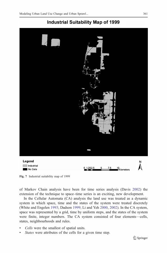
Fig. 7 Industrial suitability map of 1999

Modeling Urban Land Use Change and Urban Sprawl... 361

& Relationships among the cells were defined within neighbourhoods. The nextstate of each cell was determined by the states of its neighboring cells.

& Rules were used to define the states of the cells in the next time step.

In Idrisi Kilimanjaro, Cellular Automata analysis is accomplished by theCA_Markov module, which uses the output of the Markov Chain analysis and appliesa contiguity filter to predict land use from time period two to a later time period.

To make the predictions of land use the land classifications for the six timeperiods that were produced by eCognition were imported into the Idrisi GIS as rasterfiles. For this research land use suitability was determined using the City of Calgary’sFuture Conceptual Urban Structure (FCUS; http://www.calgary.ca/docgallery/BU/

Fig. 8 Transportation suitability map of 1999

362 H. Sun, et al.

planning/pdf/calgary_plan.pdf); the location of the City within the Province ofAlberta is shown as Fig. 1). The original pdf file was converted to a .bmp file andthen to an ERDAS Imagine file in ArcCatalog. This image was classified ineCognition, exported back to an ERDAS Imagine file and reclassified as shown inTable 3.

Parks and water bodies were considered not to change during the period from1985 to 2001. Vacant area is a special class. Since the process of urban developmentis a process of consuming vacant area, vacant area in the later land use map of eachgroup was used as the suitability map of vacant area in the future. A transitionsuitability image collection was created using the six suitability maps.

Fig. 9 Parks suitability map of 1999

Modeling Urban Land Use Change and Urban Sprawl... 363

2.4 Implementing the land use prediction

The trial prediction for the 1999 time period used the Markov module in Idrisi. Thisrequired a proportional error statistic to be assigned. Normally this might be difficultto determine but the City of Calgary has recently had a land use shapefile built thatindicates the date when each land use parcel was incorporated into the cityboundaries. In addition, the land use type is also indicated. For each of the six timeperiods, 4,000 random locations were generated and the Classified Data wascompared to the Reference Data from the shapefile using the PCI Geomatica V9.1software (http://www.pcigeomatics.com/). Four categories were used (residential/commercial; industrial; parks; and vacant areas) and the results recorded in an error

Fig. 10 Vacant area suitability map of 1999

364 H. Sun, et al.

(or confusion) matrix (Jensen 1996) where diagonal entries indicate an accurateclassification. The overall accuracy varied from a low of 89.8% for the 1992 imageto a high of a 92.5% for the 2001 image, while the average for the six images was91.3%.

This accuracy assessment was used to set the proportional error parameter at 0.1during the running of the Markov and CA_Markov modules. The initial analysisused the 1985 and 1992 classified images to “predict” the 1999 land use patternbased on Idrisi’s default contiguity filter. Once this had been deemed to be a successa “real” prediction for the year 2010 was produced based on the change thatoccurred between 1990 and 2000.

Fig. 11 Water bodies suitability map of 1999

Modeling Urban Land Use Change and Urban Sprawl... 365

2.5 The measurement of urban sprawl using Shannon’s entropy

Urban sprawl is a complex phenomenon, which not only has environmental impacts,but also social impacts (Barnes et al. 2001; www.sprawlwatch.org/). Due to itscomplexity, there is no specific, measurable, and generally accepted definition ofurban sprawl (Sutton 2003). Many attempts have been made to measure urbansprawl (Ewing,1997; Nelson 1999; Galster et al. 2000; Yeh and Li 2001; Sudhira etal. 2004). The percentage of an area covered by impervious surfaces and concrete isa straightforward measure of urban development (Barnes et al. 2001). Based on thisidea, Shannon’s Entropy, when integrated with GIS, has proved to be a simple butefficient approach for the measurement of urban sprawl (Shekhar 2004).

Since there were six land use maps derived from the object-oriented classification,in order to make the measurement of the 6 years of sprawl comparable, relativeentropy instead of standard entropy was utilized because the range of relativeentropy is always between 0 and 1. Relative entropy (En) can be expressed in thisformula:

En ¼Xn

i

pi log 1=pið Þ=log nð Þ ð1Þ

Where pi ¼ xi

�Pn

ixi and xi is the density of land development, which equals the

amount of built-up land divided by the total amount of land in the ith zone in thetotal of n zones. The number of zones means the number of buffer zones aroundthe city center (22, 1 km concentric rings around the downtown area were neededto cover all parts of the city) or around selected roads (Yeh and Li 2001).

Since entropy can be used to measure the distribution of a geographicalphenomenon, the difference in entropy between two different periods of time canalso be used to indicate the change in the degree of dispersal of land development orurban sprawl (Yeh and Li 2001).

ΔEn ¼ En t þ 1ð Þ � En tð Þ ð2Þ

WhereΔEn is the difference of the relative entropy values between two time periods,En(t+1) is the relative entropy value at time period t+1,En(t) is the relative entropy value at time period t.In this case, six land use maps had been derived from the classification

process. The only task left for calculating the entropy was to create the buffer

Table 4 Transition areas matrix

Expected to transition to

Cells in Residential and commercial Industrial Transportation Parks Vacant area Water bodies

Residential and commercial 205600 0 47 0 38878 482Industrial 0 39606 0 0 5045 0Transportation 0 0 46182 0 5152 0Parks 350 350 350 15760 350 350Vacant area 83837 5957 2653 0 414966 2530Water bodies 839 0 0 0 560 12133

The diagonal elements of the matrix indicate no change in land use between the two time periods.

366 H. Sun, et al.

zones. Accurate data for roads for all 6 years were not available for thisproject, but fortunately, Calgary has a very clearly defined downtown area.So, Shannon’s Entropy was computed on the basis of the buffer zones aroundthe town center.

Fig. 12 Predicted land use map of 1999

Modeling Urban Land Use Change and Urban Sprawl... 367

3 Results

3.1 Land use classification and prediction

Each satellite image was segmented into three levels for the purpose ofclassification. An example, of these three levels for the 2001 image is shown asFigs. 2, 3, and 4. Figure 5 shows the Land Use Classification Results for 2001 asproduced by the eCognition software.

The ASCII eCognition file was then exported into the Idrisi software and converted tothe Idrisi raster format so that the land use prediction could be carried out using the IdrisiKilimanjaro software as described above. In order to make the process operational,suitability maps were created to display the future development for each of the three landuse classes: transportation network; residential and commercial; and industrial. Thesethree land use classes were extracted from the FCUS Map mentioned above.

In order to produce the prediction for 1999 six suitability maps had to be created,one for each of the following six land use classes: residential and commercial(Fig. 6); industrial (Fig. 7); transportation network (Fig. 8); parks (Fig. 9); vacantareas (Fig. 10); and, finally, water bodies (Fig. 11). Since the latter three wereassumed not to change over the 7 years the 1992 classification results were used asthe corresponding three suitability maps. The residential and commercial suitabilitymap of 1999 was created by subtracting the residential and commercial map of 1992from the residential and commercial map for the future (i.e., the FCUS Map referredto above). The industrial suitability map of 1999 was created in the same way. Thetransportation in the future map was used directly as the transportation suitabilitymap of 1999. The resulting six suitability maps were collected together using Idrisi’sCollection Editor to produce a transition suitability image collection for use inIdrisi’s CA_Markov module.

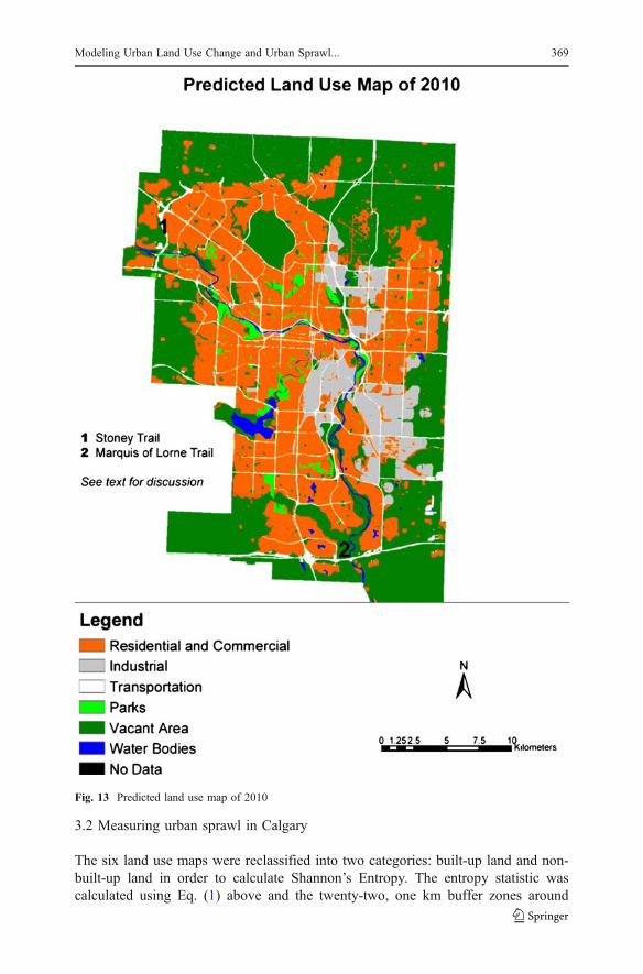
Table 4 shows the transition areas matrix produced by running Idrisi’s Markovmodule. The off-diagonal elements indicate the number of cells that are expected tochange from each existing land use class in 1985 to each new class in 1992. Usingthe 1985 and 1992 land use maps, the transition areas matrix and the transitionsuitability collection, Idrisis’s CA_Markov module was used to simulate the land usepattern of 1999 (Fig. 12). In order to compare the 1999 “prediction” with the actualland use in that year, Idrisi’s Validate module was used to calculate the Kno,Klocation and Kquantity values. Respectively, these were 0.93, 0.92 and 0.98(Table 5). Values above 0.9 indicate good agreement between the actual andpredicted maps (Pontius 2000). Since the land use prediction of 1999 was sosuccessful, the land use prediction of 2010 was implemented in the same way. Theresult is shown in Fig. 13.

Table 5 Results of the validation analysis (see text for discussion)

Variations Formula Values

KnoPo�NQNL1�NQNL 0.9293

Klocation Po�MQNLMQPL�MQNL 0.9194

Kquantity Po�NQMLPQML�NQML

0.9826

368 H. Sun, et al.

3.2 Measuring urban sprawl in Calgary

The six land use maps were reclassified into two categories: built-up land and non-built-up land in order to calculate Shannon’s Entropy. The entropy statistic wascalculated using Eq. (1) above and the twenty-two, one km buffer zones around

Fig. 13 Predicted land use map of 2010

Modeling Urban Land Use Change and Urban Sprawl... 369

Calgary’s downtown core (Fig. 14). The map of the built-up land is shown asFig. 15. The results of the entropy calculation are shown in Table 6 and Fig. 16 andthe change in the entropy measure is shown in Table 7 and Fig. 17.

4 Discussion

4.1 The process of land use classification

The object oriented classification approach used in the eCognition softwaresuccessfully avoided the so-called “salt-and-pepper” effect that commonly resultswhen pixel-based remote sensing classification approaches are used.

The multiresolution segmentation approach used by eCognition aided the processof classification by allowing the object mean value for the urban area to be used todistinguish the rural area beyond the city limits. The eCognition software has six

Fig. 14 Buffer zones around downtown Calgary

370 H. Sun, et al.

parameters that can be adjusted in the multiresolution segmentation process.Although this increases the flexibility and adaptability of the software to variousenvironments the choice of values to be entered for these parameters is not alwaysstraightforward and may require the use of additional local knowledge that is notalways available (Flanders et al. 2003). Only six classes could be extracted using thespectral information from the images. This research showed that the eCognitionsoftware is a powerful tool for image classification but that its use requiresconsiderable trial-and-error manipulation of the input parameters.

Fig. 15 Built-up land and non built-up land of 2001

Modeling Urban Land Use Change and Urban Sprawl... 371

4.2 The limits to land use prediction

The suitability maps used in this research had a great influence on the land usepredictions. This is because they act as the rules for the CA model. Different mapswill lead to different rules that in turn may produce totally different results. Thesensitivity of the predictions to the suitability maps will require further research.

Although the procedures used in the Markov Chain analysis in this researchproved to be an effective approach for calculating the land use transitionprobabilities, these procedures assumed that the transition probabilities do notchange over time. In other words, Markov Chain analysis predicts the future land usepattern only on the basis of the known land use patterns of the past. This is aweakness of the method in terms of simulating urban growth since new influenceson the urban structure cannot be evaluated.

Although Table 5 (see Section 3.1) gave strong evidence that the predicted landuse map of 1999 was similar to the actual land use map of 1999 it is still easy to seediscrepancies between the two maps. Many commercial and residential landdevelopments that occurred along the edge of the built-up area between 1992 and1999 were not predicted precisely by the CA model. The predicted land use map of1999 did show a number of development trends that can be found on the actual landuse map of 1999. For example, the predicted map showed there would be residentialand commercial land development between Harvest Hills Boulevard and DeerfootTrail (Highway 2) along Country Hills Boulevard in the extreme northern-centralregion of the map (Fig. 12). In reality, the land development not only happenedthere, but also grew faster than the prediction. Such examples can also be found inother places around the city. These underestimates indicate that the residential andcommercial land was developed faster from 1992 to 1999 than from 1985 to 1992,confirming the weakness of the Markov Chain Analysis that was noted above.

Table 6 Shannon’s Entropy values of Calgary in the 6 years

Year

1985 1990 1992 1999 2000 2001

0.850928091 0.86418883 0.860065433 0.886924987 0.891793962 0.905053353

Six Years' Relative Entropy Values

0.82

0.84

0.86

0.88

0.9

0.92

1985 1990 1992 1999 2000 2001

Year

En

Fig. 16 Six years’ relative entropy values

372 H. Sun, et al.

The shape of the contiguity filter used in this analysis may have influenced the resultsof the simulation. The filter develops a spatially-explicit weighting factor which will beapplied to each of the suitability maps, weighting more heavily areas that are next toexisting land uses. This ensures that land use change occurs next to existing similar landuse classes, and is not wholly random (Eastman 2003). Due to the nature of thecontiguity filter, the land that was deemed suitable for industrial and commercialdevelopment on the FCUS map did not always receive the expected development inthe simulation and the converse was also true. A different filter with a different set ofweights might have produced different results and again research on the sensitivity ofthe results to various weightings for the contiguity filter is warranted.

A much clearer trend can be detected when comparing the predicted land use mapof 2010 with the land use map of 2000. In the Northwest quadrant the residential andcommercial land would be further developed in the northwest direction, in theNortheast quadrant development will occur in a northerly direction and in theSoutheast quadrant it will move due east. Industrial land is expected to expand onthe city’s eastern edge. Stoney Trail, a major in-city freeway on the western side ofthe city, and the Marquis of Lorne Trail, an east–west freeway in the extreme southof the city, (see Fig. 13) were predicted to become more important links in Calgary’stransportation network. Although it is impossible to evaluate how accurate theprediction for 2010 is, it did yield some suggestions about where the city willdevelop in the next several years.

4.3 The on-going rise of urban sprawl

The calculation of Shannon’s entropy measure indicated that Calgary was continuingto sprawl between 1985 and 2001. The entropy value for 1992 is a little lower than

Table 7 Differences of Shannon’s Entropy

Time period ΔEn

1990–1985 0.0132607391992–1990 −0.0041233971999–1992 0.0268595542000–1999 0.0048689752001–2000 0.013259391

Differences of Relative Entropy Values in Each Pair of Years

-0.01-0.005

00.0050.01

0.0150.02

0.0250.03

1990-1985 1992-1990 1999-1992 2000-1999 2001-2000

Time Period

ΔE

n

Fig. 17 Differences of relative entropy values in each pair of years. (The sign “−” means minus.)

Modeling Urban Land Use Change and Urban Sprawl... 373

that of 1990. This is probably a result of the incompleteness of the 1992 image. Incomparison to the 1993 average relative entropy value of 0.767, calculated by Yehand Li (2001) for the 24 buffer zones around the 29 towns of Dongguan City inGuangdong Province in China, all 6 entropy values for Calgary are higher. Thisimplies that urban sprawl in Calgary was a far more serious matter than that detectedby Yeh and Li in their study.

Given an existing set of land development policies or lack thereof, the drivingforce behind urban sprawl in Calgary is population growth. Figure 18 showsCalgary’s population growth between 1985 and 2001 demonstrating a strongcorrelation with the growth of sprawl.

Urban sprawl is occurring around the world. In recent years, the negative socialand environmental effects of urban sprawl have been realized by more and moreresearchers and city planners. Smart Growth is a policy oriented strategy for fightingsprawl (Freilich 1999) and is primarily based on the implementation of higherresidential densities (Danielson et al. 1999). This approach to combating urbansprawl now has a strong advocacy presence on the Internet (www.smartgrowth.org/).Faced with ongoing urban sprawl and strong population growth, the City of Calgaryneeds to consider smart growth policies to encourage the efficient and effective useof newly developed land or the re-use of established land. The City of Calgary’s newemphasis on Transit Oriented Design where higher residential densities are promotedaround light rail transit stations is a new policy that may do much to reverse thehistoric trend toward urban sprawl (www.calgary.ca/DocGallery/BU/planning/pdf/3405_tod_policy_guidelines.pdf). Our results suggest that while Calgary’s mayor,Dave Bronconnier, is correct in his assertion that urban sprawl was a problem in the1980s he is incorrect in assuming that the problem has been dealt with and that itwill not be a concern for the future (Graveland 2006).

5 Conclusions

This paper has demonstrated a methodology for producing land use classificationfrom Landsat images using the object-oriented methodologies contained in the

Population of Calgary

0

100000

200000

300000

400000

500000

600000

700000

800000

900000

1000000

1985 1990 1992 1999 2000 2001

Year

Pop

ulat

ion

Fig. 18 Population of Calgary from 1985 to 2001

374 H. Sun, et al.

eCognition software. The classified images were then used to predict future land usechange in the City of Calgary, Alberta, using Markov Chain analysis and CellularAutomata approaches based on the interactions between the transportation networkand various other types of land use. Shannon’s entropy statistic was used to measurethe degree of sprawl in the city. This was shown to be high and increasing. SmartGrowth policies were advocated as a remedy to problems generated by high rates ofurban sprawl. Models such as those described here can provide simulated inputs forthe variables commonly used in the four step transportation planning process.

Acknowledgements The authors would like to acknowledge the assistance of Bart Hulshof, MGISGeomatics Technician in the Department of Geography. The land use shapefile that was used in theaccuracy assessment was supplied by Matthew Sheldrake, MSc. graduate from the Department ofGeography, University of Calgary.

References

Barnes KB III, Morgan JM, Roberge MC, Lowe S (2001) Sprawl development: its patterns, consequences,and measurement. Towson University, Towson. http://chesapeake.towson.edu/landscape/urbansprawl/download/Sprawl_white_paper.pdf

Benenson I, Torrens PM (2004) Geosimulation: automata-based modeling of urban phenomena. Wiley,Chichester

Benz UC, Hofmann P, Willhauck G, Lingenfelder I, Heynen M (2004) Multi-resolution, object-orientedfuzzy analysis of remote sensing data for GIS-ready information. ISPRS J Photogramm Remote Sens58:239–258

Boyce D, Bar-Gera H (2004) Multiclass combined models for urban travel forecasting. Netw Spat Econ4:115–124

Dadson S (1999) Cellular automata and spatial self-organization in GIS. http://www.geog.ubc.ca/courses/geog516/notes/catalk.html

Danielson KA, Lang RE, Fulton W (1999) Retracting suburbia: smart growth and the future of housing.Hous Policy Debate 10:513–540

Davis JC (2002) Statistics and data analysis in geology, 3rd edn. Wiley, New YorkDavis AA (2006) Sprawlicide Avenue, May, 38–45Definiens Imaging GmbH (2002) eCognition user guide 3. Definiens Imaging GmbH, München, GermanyEastman JR (2003) Idrisi Kilimanjaro tutorial. Clark Labs, Clark University, Worcester, MAEspino R, de Ortuzar JD, Roman C (2006) Confidence interval for willingness to pay measures in mode

choice models. Netw Spat Econ 6(2):81–96Ewing R (1997) Is Los Angeles-style sprawl desirable? J Am Plan Assoc 63:107–126Flanders D, Hall-Beyer M, Pereverzoff J (2003) Preliminary evaluation of ecognition object-based

software for cut block delineation and feature extraction. Can J Remote Sens 29:441–452Freilich RH (1999) From sprawl to smart growth-successful legal, planning, and environmental systems.

American Bar Association, ChicagoGalster G, Hanson R, Woman H, Coleman S, Friebage J (2000) Wrestling sprawl to the ground: defining

and measuring an elusive concept. Hous Policy Debate 12:681–717Graveland B (2006) Calgary contends for sprawl capital. Calg Her A8 (June 5)Jensen J (1996) Introductory digital image processing. Prentice Hall, New JerseyLi X, Yeh AG (2000) Modelling sustainable urban development by the integration of constrained cellular

automata and GIS. Int J Geogr Inf Sci 14:131–152Li X, Yeh AG (2002) Neural-network-based cellular automata for simulating multiple land use changes

using GIS. Int J Geogr Inf Sci 16:323–343Marchal F (2005) A trip generation method for time-dependent large-scale simulations of transport and

land-use. Netw Spat Econ 5:179–192Nelson AC (1999) Comparing states with and without growth management analysis based on indicators

with policy implications. Land Use Policy 16:121–127

Modeling Urban Land Use Change and Urban Sprawl... 375

Nie X, Zhang JM (2005) A comparative study of some macroscopic link models used in dynamic trafficassignment. Netw Spat Econ 5:89–115

Pontius RG Jr (2000) Quantification error versus location error in comparison of categorical maps.Photogramm Eng Remote Sensing 66:1011–1016

Proudfoot WA (2004) Evaluation of eCognition for extraction of wetland and drainage features. MGISProject. Dept. of Geography, University of Calgary, Calgary, Alberta

Shekhar S (2004)Urban sprawl assessment entropy approach. GISDevelopment, http://www.gisdevelopment.net/magazine/gisdev/2004/may/urban.shtml

Sudhira HS, Ramachandra TV, Jagadish KS (2004) Urban sprawl: metrics, dynamics and modeling usinggis. Int J Appl Earth Observ Geoinformation 5:29–39

Sutton PC (2003) A scale-adjusted measure of “urban sprawl” using night time satellite imagery. RemoteSens Environ 86:353–369

Waddell P, Borning A, Noth M, Frier N, Becke M, Ulfarsson G (2003) Microsimulation of urbandevelopment and location choices: design and implementation of UrbanSim. Netw Spat Econ 3:43–67

White R, Engelen G (1993) Cellular automata and fractal urban form: a cellular modeling approach to theevolution of urban land use patterns. Environ Plann A 25:1175–1199

Yeh AG, Li X (2001) Measurement and monitoring of urban sprawl in a rapidly growing region usingentropy. Photogramm Eng Remote Sensing 67:83–90

376 H. Sun, et al.