MODELING URBAN SPRAWL AND LAND USE CHANGE IN A COASTAL AREA

–A NEURAL NETWORK APPROACH

HUIYAN LINDepartment of Applied Economics and StatisticsClemson University, Clemson, SC 29634Email: huiyanl@clemson.edu

KANG SHOU LUStrom Thurmond InstituteClemson University, Clemson, SC 29634Email: klu@strom.clemson.edu

MOLLY ESPEYDepartment of Applied Economics and StatisticsClemson University, Clemson, SC 29634Email: mespey@clemson.edu

JEFFERY ALLENStrom Thurmond InstituteClemson University, Clemson, SC 29634Email:jeff@strom.clemson.edu

Paper prepared for presentation at the American AgriculturalEconomics Association Annual Meeting, Providence,

Rhode Island,July 24-27, 2005

Copyright 2005 by Huiyan Lin, Kang Shou Lu, Molly Espey, and JefferyAllen. All rights reserved. Readers may make verbatim copies of thisdocument for non-commercial purposes by any means, provided that thiscopyright notice appears on such copies.

brought to you by COREView metadata, citation and similar papers at core.ac.uk

provided by Research Papers in Economics

1

ABSTRACT

Complexity of urban systems necessitates the consideration of interdependency among

various factors for land use change modeling and prediction. The objective of this study

is to explore the applicability of computational neural networks in modeling urban sprawl

and land use change coupled with geographic information systems (GIS) in Hilton Head

Island, South Carolina. We are particularly interested in the capabilities of neural

networks to identify land use patterns, to model new development, and to predict future

change. A binary logistic regression model is estimated comparison. The results indicate

the neural network model is an improvement over the logistic regression model in terms

of prediction accuracy.

Keywords: urban sprawl, land use change, neural networks, logistic regression model.

2

1. Introduction

Coastal ecosystems serve human societies in multiple beneficial ways. They are

the main source of seafood and they provide recreation and aesthetic value. South

Carolina is the nation’s second largest coastal resort state in terms of beach destination

trips, superseded only by Florida. Coastal tourism in this state creates about 4.2 billion

dollars of revenue annually (World Travel & Tourism Council 2001). Unfortunately,

coastal ecosystems have been deteriorating due to conversion of agricultural and forest

land for residential development throughout this area, both in the form of intensive

subdivisions as well as large-lot dispersed residential parcelization. As sustainable

development becomes a goal for many coastal communities and the continuing coastal

change connected with accelerated growth becomes a critical issue, urban sprawl in

coastal areas has drawn more public attention and scholars’ interests. Although the

logistic framework has been used in many conventional models of land use change due to

its capabilities of handling discrete land use variables and the mix of both discrete land

use variables and continuous independent variables, it has shown limited success in

predicting land use change in complex urban systems, especially in the coastal area where

tourism development and associated commercial and residential growth are dramatic.

Landis (1994) has shown that the logistic framework does not always provide satisfactory

predictions due to the complexity of urban land use systems and limitations of the model.

In addition, changes in urban land use systems demonstrate both regularity and

irregularity in temporal rate and spatial patterns.

As a powerful tool to quantify and model complex behavior and patterns, the use

of neural network models has increased substantially over the last several years. Fischer

3

(2001) states that neural networks offer four primary attractions which distinguish them

qualitatively from the current standard approaches: machine learning, speed of

computation, greater representational flexibility and freedom from linear model design.

This paper applies neural network model to predict urban growth in the Hilton Head

Island, South Carolina, and both spatial and temporal sample datasets are used to test its

reliability and validity against the logistic regression.

2. Background

2.1. Land Use Change Model

Modeling land use change essentially started in the 1950s, demonstrated less

activity in the 1970s and 1980s. However, it has been revived intensely in the 1990s as a

result of the improvement in spatial data availability and advancements in computer

technologies and geographic information systems (GIS) (Wegener 1994). Two basic

types of spatially explicit land use change models were characterized by Theobald and

Hobbs (1998): regression-type models and spatial transition-based models. The

regression-type models of land use change are useful in exploring the various social,

economic, and spatial variables that drive change and are useful in evaluating the impacts

of alternative policies on land use and development patterns. The relative contribution of

different variables for predicting land used change can be easily attained under the

regression-type model. Bockstael (1996), Carrión-Flores and Irwin (2004) have

employed probability models of factors affecting land use change at the rural-urban

fringe. Hite et al. (2003) have investigated the impact of a number of factors that promote

land use change by using competing risks survival models. The spatial transition models

4

are an extension of the aspatial Markov technique and a form of stochastic cellular

automata. Clarke et al. (1997) employed cellular automata to predict emergent behaviors

and patterns that were more complex than those generated by simple equilibrium models.

Integration with GIS is essential for modeling land use changes because of the

spatial nature of many the input variables. Most GIS-based models of land use change

employ data stored in the raster data structure (Clarke et al., 1997) because the

representation of space is simplified by breaking it into many units of equal size and

shape. Lu and Allen (2003) proposed a GIS-based integrated approach to model and

predict urban growth in terms of land use change in the Myrtle Beach region of South

Carolina.

2.2. Neural Networks with Land Use Modeling

The techniques of artificial neural networks have been intensively employed in

many disciplines by the recognition that human brain computes in a highly complex,

nonlinear and parallel way which is entirely different from the conventional digital

computer. They are used in pattern recognition (Le Cun et al., 1990), climate forecasting

(Drummond, Joshi, and Sudduth, 1998), medicine (Hechlt-Nilsen, 1990), speech

production and recognition (Lippmann, 1989), business (Fishman et al., 1991) and

control (Nguyen & Widrow, 1989). However, neural networks were not used in the field

of land use modeling and resource management until the mid-1990s. Wang (1994) used

artificial neural networks in a geographical information system for agricultural land

suitability assessment. Gimblett et al. (1994) developed a forest management decision

model based on neural network and tested the model in the Hoosier National Forest. Most

5

recently, Yeh and Li (2002) used neural networks and cellular automata to simulate

potential urban development patterns.

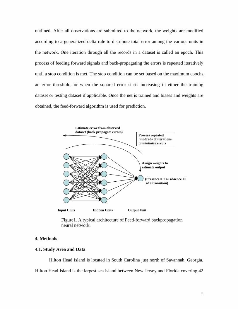
3. Computational Neural Networks

A multi-layer, multi-units back-propagation neural net was constructed based on

the methodology of computational neural networks developed by Fischer (2001). The net

contains an input layer with multiple units, a hidden layer with multiple units, and an

output layer with only one unit. Figure 1 shows a typical feed-forward back-propagation

neural network.

The training of such a network involves three phases: the feedforward of the input

training pattern, the back propagation of the associated error, and the adjustment of the

weights. Units between two adjacent layers are interconnected. Each unit from the input

layer sends its signal to each unit of the hidden layer. Each input unit receives signal and

broadcasts this signal to each of the hidden units. Each hidden unit sums the signal with

different weights, then applies its activation function to compute its output signal, and

sends this signal to the unit in the output layer. Binary sigmoid function, one of the most

typical activation functions, is used in this study and has range of (0, 1). The output unit

receives a signal from each hidden layer and sums the signals with corresponding weights

and computes the output. This process can repeat if there are more hidden layers. The

weights can be determined using the robust back-propagation algorithm. The algorithm

randomly chooses the initial weights, and compares the calculated output for a given

observation with the expected output for that observation. Using the mean squared error,

the difference between the expected and calculated output values across all observation is

6

outlined. After all observations are submitted to the network, the weights are modified

according to a generalized delta rule to distribute total error among the various units in

the network. One iteration through all the records in a dataset is called an epoch. This

process of feeding forward signals and back-propagating the errors is repeated iteratively

until a stop condition is met. The stop condition can be set based on the maximum epochs,

an error threshold, or when the squared error starts increasing in either the training

dataset or testing dataset if applicable. Once the net is trained and biases and weights are

obtained, the feed-forward algorithm is used for prediction.

4. Methods

4.1. Study Area and Data

Hilton Head Island is located in South Carolina just north of Savannah, Georgia.

Hilton Head Island is the largest sea island between New Jersey and Florida covering 42

(Presence = 1 or absence =0of a transition)

Input Units Hidden Units Output Unit

Assign weights toestimate output

Process repeatedhundreds of iterationsto minimize errors

Figure1. A typical architecture of Feed-forward backpropagationneural network.

Estimate error from observeddataset (back propagate errors)

7

square miles (12 miles long and 5 miles wide at its widest point). Its largest industry by

far is tourism with broad beaches on its ocean side. Hilton Head has 14 miles of beaches,

two dozen golf courses in the immediate area, hundreds of tennis courts, and about 200

restaurants. About 2.2 million resort guests visit Hilton Head Island annually (its

permanent population is about 34,000).

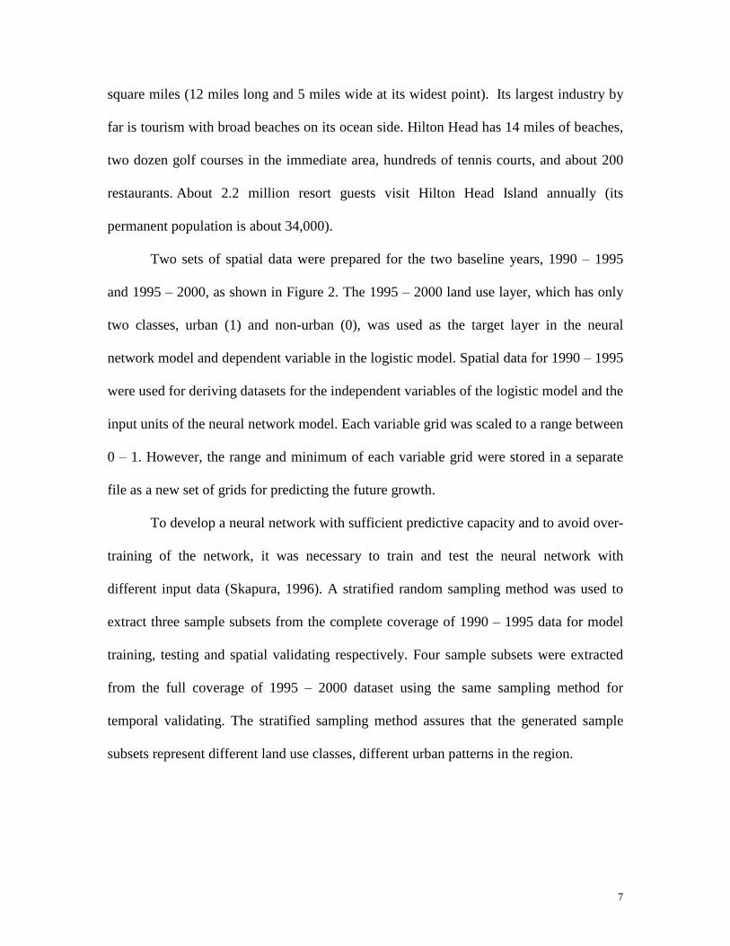
Two sets of spatial data were prepared for the two baseline years, 1990 –1995

and 1995–2000, as shown in Figure 2. The 1995–2000 land use layer, which has only

two classes, urban (1) and non-urban (0), was used as the target layer in the neural

network model and dependent variable in the logistic model. Spatial data for 1990–1995

were used for deriving datasets for the independent variables of the logistic model and the

input units of the neural network model. Each variable grid was scaled to a range between

0 –1. However, the range and minimum of each variable grid were stored in a separate

file as a new set of grids for predicting the future growth.

To develop a neural network with sufficient predictive capacity and to avoid over-

training of the network, it was necessary to train and test the neural network with

different input data (Skapura, 1996). A stratified random sampling method was used to

extract three sample subsets from the complete coverage of 1990 –1995 data for model

training, testing and spatial validating respectively. Four sample subsets were extracted

from the full coverage of 1995 –2000 dataset using the same sampling method for

temporal validating. The stratified sampling method assures that the generated sample

subsets represent different land use classes, different urban patterns in the region.

8

4.2. Operational Model Design

A neural net was constructed to predict the land transformation from the rural

state to urban use. Land use as the only output unit was classified into two categories:

urban (1) and rural (0). Figure 3 illustrates a neural network land use model suitable to

the unique environment of the Hilton Head Island, South Carolina. For logistic regression

model and neural network in this study, a total of 11 predictor variables (input units for

neural network) are used which represent the potential key factors that affect land use and

urban growth. The predictor variables are grouped into 3 categories: physical suitability,

services accessibility, and neighborhood characteristics. Physical suitability includes

parcel lot size, slope of parcel, and elevation of parcel. Services accessibility includes

distance to major roads, distance to golf courses, distance to water lines, distance to

Figure 2. Location of Hilton Head Island, SC and Land Use Changes.

9

ocean front, distance to bay front, distance to road, and distance to parks. Neighborhood

characteristics include distance to existing urban. Units of the hidden layer can be set

during the training process. But for simplicity, 11 hidden units were used in the final

model. Binary sigmoid function is used as the activation function to make the results

comparable with those of logistic regression model which fall between 0 and 1.

Prediction of land use change with neural network involves four stages: (1) network

training using a subset of inputs from historical data (1990 –1995); (2) testing of the

network using a subset and the full set of the inputs from 1990–1995 data; (3) using the

information from the neural network to forecast land use changes from 1995 to 2000. In

addition, the results of logistic regression model are used as a benchmark for accuracy

assessment.

5. Results and Discussion

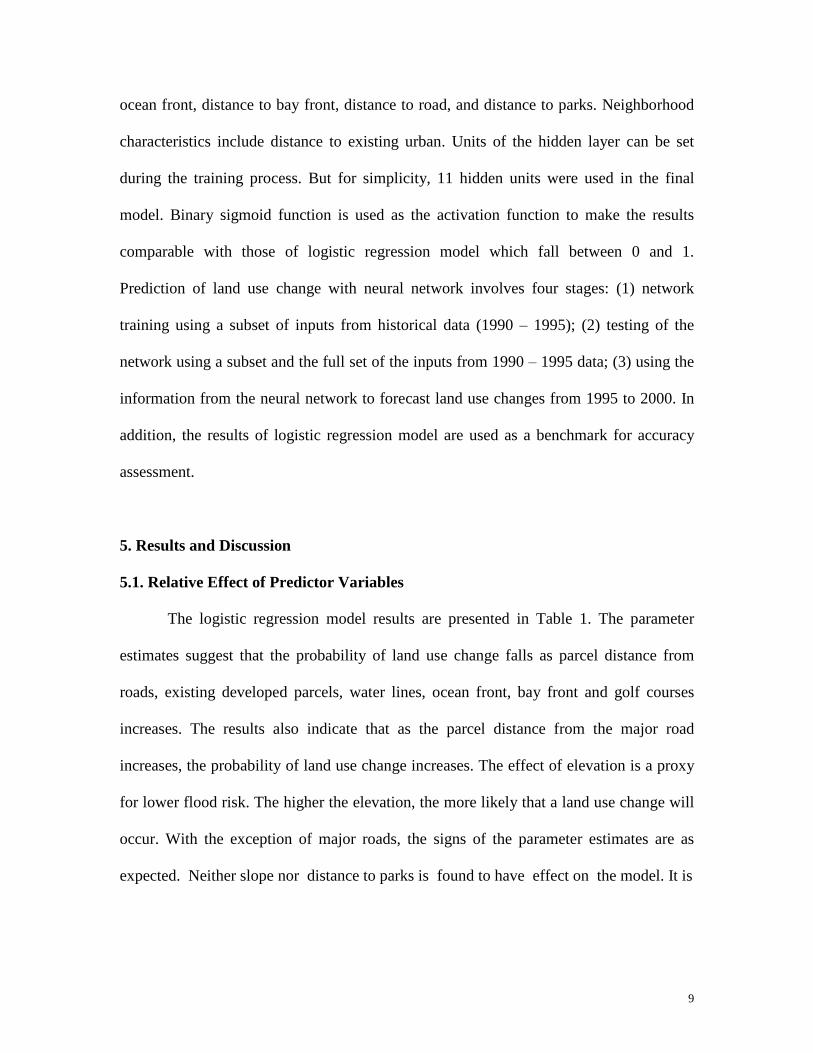
5.1. Relative Effect of Predictor Variables

The logistic regression model results are presented in Table 1. The parameter

estimates suggest that the probability of land use change falls as parcel distance from

roads, existing developed parcels, water lines, ocean front, bay front and golf courses

increases. The results also indicate that as the parcel distance from the major road

increases, the probability of land use change increases. The effect of elevation is a proxy

for lower flood risk. The higher the elevation, the more likely that a land use change will

occur. With the exception of major roads, the signs of the parameter estimates are as

expected. Neither slope nor distance to parks is found to have effect on the model. It is

10

noticeable that the physical suitability variable, parcel lot size, does not have an impact

on the land use change, perhaps because of the highly scattered feature of parcels in this

region.

Table 1. Parameter Estimates of the Logistic Regression Modelfor Hilton Head Island.

VariableParameterEstimate

StandardError

WaldChi-Square Pr>ChiSq

Constant .558 .212 6.952 .008***

D2mroad .451 .177 6.534 .011**

D2road -4.036 1.101 13.434 .000***

D2waterl -1.514 .254 35.621 .000***

D2ocean -.707 .223 10.022 .002***

D2bayfro -.490 .210 5.451 .020**

Dem 2.104 .326 41.559 .000***

Slope .596 .519 1.319 .251Lotsize 12.396 16.031 .598 .439D2park .061 .169 .128 .720D2golf -.797 .226 12.448 .000***

D2blt90 -21.418 1.098 380.340 .000***

Distance to Major Road

Distance to Water Line

Distance to Bay Front

Distance to Park

Distance to Golf Course

Distance to Ocean Front

Lot Size

Distance to Road

Distance to Existing Urban

Elevation

Slope

Land Use

•Network Architecture:11x11x1

•Activation Function: Sigmoid ƒ (x ) = 1 / [1 + exp (-x) ] ƒ′(x ) =ƒ (x ) [ 1-ƒ (x ) ]

•Training Method: StandardBackpropagation

Input Units Hidden Units Output Unit

Neural Net Model forHilton Head

Included in the model

Figure 3. Neural Network Land Use Model for Hilton Head Island, South Carolina.

11

5.1. Model Performance

As a measure of the predictive power of a discrete model, the prediction success

rates or classification accuracy is shown for the neural network model and logistic model

in Table 2 and Table 3 respectively. For each subset sample data, the two categorical

success rates (urban, non-urban) and the overall success rates were calculated for each

model. The results of classification accuracy of prediction are similar across different

datasets. The overall classification accuracy predicted by the neural network exceeds

85% while the accuracy for the rural areas is above 90% in all four cases. More

importantly, the accuracy for the urban areas is fairly good (about 80%) for a discrete

land use change model. The neural network model outperforms the logistic model in

terms of overall prediction accuracy by about 8%. The neural network model has not

done so well as logistic model in the classification of urban mainly because the majority

of the parcels (56.48%) have been developed. The logistic model tends to misclassify

parcels into the category of dominant land use. This is particularly remarkable in this area

where the adjacency to the developed parcels is the most significant predictor as

indicated by Wald coefficient of the logistic regression model. The neural network, on

the contrary, has the capability to identify these relatively isolated parcels from the

dominant land use background.

Table 2. Results of Model Training and Spatial Validation for the Neural Net (1990-1995).

Classification (N) Accuracy (%)Dataset Urban to

UrbanUrban toNonurban

Nonurbanto Urban

Nonurban toNonurban Urban Nonurban Overall

Training 2015 474 180 1817 80.96 90.99 85.42Testing 2075 454 153 1803 82.05 92.18 86.47Validating 4108 934 336 3612 81.47 92.10 86.15Full Coverage 8198 1862 649 7232 81.49 91.77 86.00

12

Table 3. Results of Model Calibration and Validation for the Logistic Model (1990-1995).Classification (N) Accuracy (%)

Dataset Urban toUrban

Urban toNonurban

Nonurbanto Urban

Nonurban toNonurban Urban Nonurban Overall

Training 2352 181 807 1145 92.85 58.66 77.97Testing 2323 186 780 1196 92.59 60.53 78.46Validating 4660 358 1555 2398 92.87 60.67 78.68Full Coverage 9335 725 3142 4739 92.79 60.13 78.45

The results of temporal validation from 1995-2000 for both models are

summarized in Table 4 and Table 5. They demonstrate the same patterns as the spatial

validation indicates from the training dataset for 1990-1995, but the difference in

prediction accuracy between the two models is less impressive. However, prediction

accuracy for each land use category varies substantially between the two different tests

(spatial and temporal) for the logistic regression model but remains almost the same for

the neural network. It may suggest that the neural network is more stable for predicting

temporal land use changes.

Table 4. Results of Temporal Validation for the Neural Net (1995-2000).Classification (N) Accuracy (%)

Dataset Urban toUrban

Urban toNonurban

Nonurbanto Urban

Nonurban toNonurban Urban Nonurban Overall

Sample 1 2405 633 68 1380 79.16 95.30 84.37Sample 2 2419 612 38 1416 79.81 97.39 85.51Sample 3 4851 1315 113 2691 78.68 95.97 84.08Full Coverage 9675 2560 219 5487 79.08 96.16 84.51

Table 5. Results of Temporal Validation for the Logistic Model (1995-2000).Classification (N) Accuracy (%)

Dataset Urban toUrban

Urban toNonurban

Nonurbanto Urban

Nonurban toNonurban Urban Nonurban Overall

Sample 1 2588 450 299 1149 85.19 79.35 83.30Sample 2 2610 421 249 1205 86.11 82.87 85.06Sample 3 5262 904 567 2237 85.34 79.77 83.60Full Coverage 10460 1775 1115 4591 85.49 80.46 83.89

13

The actual and predicted landscapes for the period from 1995 to 2000 are

illustrated in Figure 4 and Figure 5 respectively. In visually comparing the observed and

predicted land use patterns, both logistic and neural network models perform reasonably

well. The resulting display confirms that the predicted pattern without agglomerative

effects from adjacent existing parcel development is more scattered. It also shows the

expected pattern of urban sprawl which moves from ocean side to inland. However, it is

found that the logistic model over-predicts the amount of urban sprawl and demonstrates

more predicted error distribution. It is noticeable that neither model is able to generate

good prediction for the area that has experienced dramatic development in the middle

part of the Hilton Head Island in 1995. This suggests that there might be a need of

involvement for other non-statistical methods or empirical models.

14

Figure 4. Observed and Predicted of Land Use Patterns by Logistic RegressionModel for Hilton Head Island, SC, 1995-2000.

15

Figure 5. Observed and Predicted of Land Use Patterns by Neural NetworkModel for Hilton Head Island, SC, 1995-2000.

16

Table 6 and Figure 6 provide some of the critical values that helps determine the

classification strategies. As shown in Figure 6, the classification accuracy for each of the

three categories (urban, rural, overall) varies with the cutoff value used: classification

accuracy for urban use declines from 100% to 0 %as the cutoff value changes from 0 to 1;

Classification accuracy for rural use increases from 0% to 100% as the cutoff value

moves from 0 to 1; The maximum overall accuracy tends to occur where the cutoff value

is close to 0.5; There is a point (three-way tie point) where all three curves intersect with

equal values. The neural net also demonstrated a certain degree of superiority over the

logistic model in terms of maximum overall classification accuracy by about 4% and

three-way tie accuracy. The convex curve of urban classification based on the neural net

prediction implies a relative small chance for classification error, compared to the curve

based on the logistic prediction. All these indicate that prediction based on neural

network is more stable and thus more reliable which has significant implications when

different classification strategies are applied.

Table 6. Critical values of classifications based on the probabilities predicted by theNeural Net and the Logistic Model.

The Neural Net The Logistic ModelAccuracy Cutoff Value Accuracy Cutoff Value

Urban 100% 0 100% 0Non-urban 100% 0.99 100% 0.88Overall (maximum) 87.33% 0.65 83.78% 0.61Three-way equal point 85.41% 0.37 83.51% 0.62

17

0.00 0.25 0.50 0.75 1.000

20

40

60

80

100

Acc

urac

y(%

)

Cutoff Value(A)

UrbanNonurbanOverall

0.00 0.25 0.50 0.75 1.000

20

40

60

80

100

Acc

urac

y(%

)

Cutoff Value(B)

UrbanNonurbanOverall

6. Conclusions

Land use modeling is essential to urban planning, recourse management,

landscape studies, and environmental impact analysis. A land use change model can

generate useful information regarding possible trend of future urbanization in the coastal

area. The use of an appropriate relationship model is critical for a reliable prediction of

future growth. Although the conventional logistic regression model is appropriate for

handling land use change problems, it appears insufficient to address the issue of

interdependency of the predictor variables. The alternative approach of computational

neural network examines the relationship between 11 predictor variables and urbanization,

and achieves higher overall predictive ability than the logistic regression when facing a

complex system. The next step of this study is to evaluate possible environmental impact

of future urbanization and to identify more proper social, economic and environmental

factors that affect land use and urban growth.

Figure 6. Classification Accuracy as a Function of the Cutoff Value:(A) Predicted by the Logistic Model; (B) Predicted by the Neural Net.

18

References

Bockstael, N. E. (1996). “Modeling economics and ecology: The importance of a spatial

perspective.”American Journal of Agricultural Economics, 78: 1168-1180.

Carrión-Flores, Carmen and Irwin, Elena G. (2004). “Determinants of Residential Land-

Use Conversion and Sprawl at the Rural-Urban Fringe.” American Journal of

Agricultural Economics, 86: 889-904.

Clarke, K. C., Gaydos, L., and Hoppen, S. (1997). “A self-modifying cellular automaton

model of historical urbanization in the San Francisco Bay Area.”Environment and

Planning B. 24: 247-261.

Drummond, S., Joshi, A., and Sudduth, K., (1998). “Application of Neural Networks:

Precision Farming.” IEEE Transactions on Neural Networks, 211-215.

Fischer, M.M. “Computational neural networks - Tools for spatial data analysis.”In

Fischer, M.M. and Leung, Y.(eds.): GeoComputational Modelling: Techniques and

Applications, pp. 15-34. Springer, Berlin, Heidelberg and New York, 2001.

Fishman, M., Barr, Dean S., and Loick, W. J. (1991). “Using Neural Nets in Market

Analysis.” Technical Analysis of Stocks & Commodities, 4: 18-21.

Gimblett, R. H., Ball, G. L. and Guisse, A. W. (1994). “Autonomous Rule Generation

and Assessment for Complex Spatial Modeling.” Landscape and Urban Planning.

30: 13-16.

Hecht-Nielsen, R. (1990). Neurocomputing, Addison-Wesley: Reading, MA.

Hite, D., Sohngen B. L. andTempleton, Josh. (2003). “Zoning, Development Timing,

and Agricultural Land Use at the Suburban Fringe: A Competing Risks Approach.”

Agricultural and Resource Economics Review, 32.

19

Landis, J. (1994). “The California Urban Futures Model: A New Generation of

Metropolitan Simulation Models.” Environmental and Planning B, Planning and

Design. 21: 399-420.

Le Cun, Y., B. Boser, J. S. Denker, D. Henderson, R. E. Howard, W. Hubbard, and L. D.

Jackel. (1990). “Handwritten Digit Recognition with a Backpropagation Network.”

In D. S. Touretzky, ed., Advances in Neural Information Processing Systems 2,

Morgan Kaufman, 396-404.

Limpmann, R. P. (1989). “Review of Neural Networks for Speech Recognition.”Neural

Computation, 1: 1-38.

Lu, K. S. and J. S. Allen. (2003). “Artificial Neural Net vs. Binary Logistic Regression:

Two Alternative Models for Predicting Urban Growth in the Myrtle Beach Region.”

Report Submitted to NOAA’s Land Use - Coastal Ecosystems Study (LUCES)

Program.

Nguyen, D. & B. Widrow (1989). “Fast Learning in Networks of Locally Tuned

Processing Units.”Neural Coomputation, 1: 281-294.

Skapura, D. (1996), Building Neural Networks. New Yourk: ACM Press.

Theobald, D. M., and Hobbs, N. T. (1998). “Forecasting Rural Land-use Change: a

Comparison of Regression-and Spatial Transition-based Models.”Geographical

and Environmental Modeling, 2(1): 65-82.

Wang, F. (1994). “The Use of Artificial Neural Networks n a Geographical Information

System for Agricultural Land-suitability Assessment.” Environment and Planning A,

26: 265-284.

20

Wegener, M. (1994). “Operational Urban Models: State of the Art.” Journal of the

American Planning Association, 60:17-29.

World Travel & Tourism Council. (2001). Special Country Reports, South Carolina.

London, United Kindom.

Yeh AGO, Li X. (2002). “Urban Simulation Using Neural Networks and Cellular

Automata for Land Use Planning.” In: Richardson D., Van Oosterom P. (eds)

Advances in Spatial Data Handlling. Springer, Berlin, pp 452-464.