Modelling and Multivariate Data Analysis of Agricultural Systems A thesis submitted to The University of Manchester for the degree of Doctor of Philosophy in the Faculty of Engineering and Physical Sciences 2015 Najib U Lawal School of Electrical and Electronic Engineering
Transcript
Modelling and Multivariate Data
Analysis of Agricultural Systems
A thesis submitted to The University of Manchester for the
degree of Doctor of Philosophy in the Faculty of
Engineering and Physical Sciences
2015
Najib U Lawal
School of Electrical and Electronic Engineering
2
Table of Contents
Table of Contents ................................................................................................................. 2
List of Figures....................................................................................................................... 5
List of Tables ........................................................................................................................ 7
Chapter 4 A backward Lagrangian Stochastic (bLS) model for the dispersion of Sclerotinia sclerotium spores ............................................................................................................... 88
Chapter 5 An Integrated Fault Detection, Identification and Reconstruction Scheme for Agricultural Systems ......................................................................................................... 119
Figure 3. 1: Location of Little Hoos (WGS84 Lat/Long: 51.811374/-0.373084), the experimental site, among other field trial sites at Rothamsted Research UK (source of image:
Figure 3.2: Layout of sampling area (43m by 28m) within field trial site from 31st May 2013 to 3rd June 2013 showing positions of Rotorod samplers. Data was collected at two heights of 0.8m and 1.6m (O), and additional heights of 2.4m and 3.2m (⊕). ........................... 52
An arrangement of biosensor unit, weather station and a 3D sonic anemometer were situated at the centre of the 7m-diameter ring of ascospores. Scale of sampling area excluding
upwind sampling point: 35m by 28m. All sampling positions are 7 meters apart except I, which is 14m from D. B is 1m away from the edge of the source ring. ........................... 52
canopy. (Image taken by the author). .......................................................................... 53 Figure 3. 4: Rotorod samplers at position B deployed at 0.8m (obscured), 1.6m, 2.4m and 3.2m
pictured without rain covers. Position B (as well as D) sampled at two additional heights. (Image taken by the author). ...................................................................................... 54
Figure 3. 5: A typical assembly of Rotorod sampler (1), battery (2) and Burkard timer (3), seen here only powering one sampler with its other output unused. (Image taken by author) . 55
Figure 3. 6: Biosensor attached to Uniscan potentiostat using a bespoke connector (1).
Prototype biosensor (2) sensing surface is an enzyme-coated carbon electrode (black circular area in right frame). (Image taken by author) .................................................. 59
Figure 3. 7: Biosensor calibration curve for five repeated measurements at 600C after allowing 120 seconds of mixing (𝑛 = 25, error bars = ± 1S. D. ). .................................................. 62
Figure 3.8: Oxalic acid concentrations for all days for samples collected below the OSR canopy
................................................................................................................................. 66 Figure 3.9: Oxalic acid concentrations for all days for samples collected below the OSR canopy
Figure 3.10: Side-by-side comparison of daily oxalic acid concentrations for all positions. The positions of collection of spores represent Rotorod samplers that were deployed below the
canopy. ...................................................................................................................... 68 Figure 3.11: Concentrations grouped by position for all sampling days. Spores tested for oxalic
acid were collected below the canopy. ......................................................................... 68
Figure 3.12: Along wind concentration (spore DNA) gradient below OSR canopy for first three sampling days. The key refers to field positions (letters) and height of deployment above
ground (numbers). Spore DNA axis is scaled for clarity, maximum values for the first 2 days are shown at the top and have the same units as the vertical axis. ........................ 69
Figure 3.13: Along wind concentration (spore DNA) gradient above OSR canopy for first three sampling days. Lateral (crosswind) sampling positions are not shown. ........................... 70
Figure 3.14: Wind rose showing forecasted (a) and actual (b) wind speed and directions on day
4. The forecasted wind readings were used to set the sampling axis, resulting in a misalignment of sampling grid and spore plume ........................................................... 70
Figure 3.15: The spore gradient at position B (1m downwind of spore ring) with height for first three sampling days.................................................................................................... 71
Figure 3.16: The spore gradient at position D (14m from downwind of spore ring) with height
for first three sampling days. ....................................................................................... 72 Figure 3.17: Spore dispersal gradient for all positions including crosswind (lateral) sampling
positions. The spore DNA concentration axis is in nanograms (ng) and is scaled between 0
6
to 1ng, for clarity. The key refers to field positions (letters) and height of deployment
above ground (numbers). ........................................................................................... 73 Figure 3.18: Spore DNA below the canopy plotted with distance from centre of spore ring for
first three days of sampling. Data is fitted to an inverse power law with coefficients, exponents and 𝑅2 as shown. ....................................................................................... 75
Figure 3.20: Kernel Density Estimation of spore DNA distribution below (left) and above (right)
the canopy. ................................................................................................................ 81 Figure 3.21: Dispersion contours of spore concentration below (left) and above (right) the
Figure 4.1: The assumed source configuration used for concentration footprint calculation showing approximate locations of 6 groups of Sclerotinia. Each group is assumed to cover
a 1 square meter area based on approximate measurements of area covered by fruiting bodies. The vertices of each square for the left bottom corner starting with 1 are: (-2.25,
2.5), (1.25, 2.5), (3, -0.5), (1.25, 4.0), (-2.25, -4.0), and (-4, 0.5). (Drawing not to scale)/
............................................................................................................................... 101 Figure 4.2: Normalised observations (blue asterisks) versus normalised model predictions (red
circles) above (left panels) and below (right panels) the canopy for the downwind sampling positions for all sampling days. .................................................................... 107
Figure 4.3: Normalised observations (blue asterisks) versus normalised model predictions (red circles) above (left panels) and below (right panels) the canopy for the crosswind
sampling positions for all sampling days. .................................................................... 108
Figure 4.4: Normalised observations versus normalised model predictions for all observed concentrations above the canopy. The blue line is the 1:1 line .................................... 109
Figure 4.5: Normalised observations versus normalised model predictions for all observed concentrations below the canopy. The blue line is the 1:1 line. .................................... 109
Figure 5. 1: Score plot showing first PC against second (numbers represent sample number –
hour of year) ............................................................................................................ 137 Figure 5. 2: Loading plot of first vs. second PC showing all monitoring stations (numbers
represent station numbers) ....................................................................................... 137 Figure 5. 3: Percentage of variance explained by first 20 PCs .............................................. 139
Figure 5. 4: Calibration and cross-validation errors for first 20 PCs ....................................... 139 Figure 5. 4: Missing data distribution before pre-processing ................................................ 140
Figure 5. 5: Missing data distribution after processing ......................................................... 140
Figure 5. 6: Monitor locations showing deleted monitors (red) with excessive missing data ... 141 Figure 5. 7: Score plots showing the 4 largest PCs against each other ................................. 142
Figure 5.8: Cross-validation and calibration errors .............................................................. 143 Figure 5.9: Hotelling T2 chart preliminary PCA model .......................................................... 143
Figure 5.10: SPE chart for preliminary PCA model ............................................................... 144
Figure 5. 11: Outliers from preliminary model’s SPE showing daily time of emission .............. 145 Figure 5. 12: Hotelling T2 for final PCA model .................................................................... 146
Figure 5. 13: SPE chart for final PCA model ........................................................................ 146 Figure 5. 14: Kernel density estimated distributions of Hotelling T2 and SPE ......................... 147
Figure 5. 15: KDE ICDF showing 95th percentile for Hotelling T2 and SPE ............................ 148 Figure 5. 16: Hotelling T2 control chart for new in-control samples ...................................... 149
Figure 5. 17: SPE chart for new in-control sample............................................................... 149
Figure 5. 18: Hotelling T2 control chart for in-control samples with missing data .................. 150 Figure 5. 19: SPE control chart for in-control samples with missing data .............................. 151
Figure 5. 20: Hotelling T2 chart with severe case of missing data (25%) .............................. 152 Figure 5. 21: SPE chart with severe missing data (25%) ..................................................... 153
Figure 5.22: Variable loadings on PC1 ................................................................................ 154
Table 3. 1: Volumes of oxalic acid required to prepare 50𝑚𝐿 of 0, 50, 100, 500, 1000 and
1500𝜇𝑚𝑜𝑙𝐿 − 1 standards from 10𝑚𝑚𝑜𝑙𝐿 − 1stock ....................................................... 57
Table 3.2: Current recorded biosensor measurements procedure described in section 3.3.1
Values highlighted in yellow are above baseline noise level determined in the last section and are considered positive for oxalic acid. Heights of 0.8m correspond to Rotorod
Table 3.3: Concentrations of oxalic acid measured by colourimetric analysis. Values in purple are positively and quantitatively representative of oxalic acid. Heights of 0.8m correspond
to Rotorod samplers below the canopy and all others are above the canopy (canopy height = 1m). ............................................................................................................. 65
Table 3.4: Spore DNA converted to spore numbers using 0.35pg per single spore determined by
Rogers et al. [153]. .................................................................................................... 78 Table 4. 1: Table of model parameters. ............................................................................. 105
Table 4.2: Calculated model performance measures for different observation groups (above or below canopy height). Number of observations is shown in square brackets ................ 111
Table 5. 2: Index of variables and sample number of corrupted observations ....................... 133
Table 5. 2: Control charts with increasing missing data ....................................................... 151 Table 5.3: Augmented MSPC results showing deviation of corrupted variables from their kriged
estimates and the kriging estimator’s variance ............................................................ 159
8
Abstract
Najib Lawal
Modelling and multivariate data analysis of agricultural systems
The University of Manchester (2015) The broader research area investigated during this programme was conceived from a goal to
contribute towards solving the challenge of food security in the 21st century through the reduction
of crop loss and minimisation of fungicide use. This is aimed to be achieved through the introduction of an empirical approach to agricultural disease monitoring. In line with this, the
SYIELD project, initiated by a consortium involving University of Manchester and Syngenta, among others, proposed a novel biosensor design that can electrochemically detect viable
airborne pathogens by exploiting the biology of plant-pathogen interaction. This approach offers
improvement on the inefficient and largely experimental methods currently used. Within this context, this PhD focused on the adoption of multidisciplinary methods to address three key
objectives that are central to the success of the SYIELD project: local spore ingress near canopies, the evaluation of a suitable model that can describe spore transport, and multivariate analysis of
the potential monitoring network built from these biosensors. The local transport of spores was first investigated by carrying out a field trial experiment
at Rothamsted Research UK in order to investigate spore ingress in OSR canopies, generate
reliable data for testing the prototype biosensor, and evaluate a trajectory model. During the experiment, spores were air-sampled and quantified using established manual detection methods.
Results showed that the manual methods, such as colourimetric detection are more sensitive than the proposed biosensor, suggesting the proxy measurement mechanism used by the biosensor
may not be reliable in live deployments where spores are likely to be contaminated by impurities
and other inhibitors of oxalic acid production. Spores quantified using the more reliable quantitative Polymerase Chain Reaction proved informative and provided novel of data of high
experimental value. The dispersal of this data was found to fit a power decay law, a finding that is consistent with experiments in other crops.
In the second area investigated, a 3D backward Lagrangian Stochastic model was
parameterised and evaluated with the field trial data. The bLS model, parameterised with Monin-Obukhov Similarity Theory (MOST) variables showed good agreement with experimental data and
compared favourably in terms of performance statistics with a recent application of an LS model in a maize canopy. Results obtained from the model were found to be more accurate above the
canopy than below it. This was attributed to a higher error during initialisation of release velocities below the canopy. Overall, the bLS model performed well and demonstrated suitability for
adoption in estimating above-canopy spore concentration profiles which can further be used for
designing efficient deployment strategies. The final area of focus was the monitoring of a potential biosensor network. A novel
framework based on Multivariate Statistical Process Control concepts was proposed and applied to data from a pollution-monitoring network. The main limitation of traditional MSPC in spatial
data applications was identified as a lack of spatial awareness by the PCA model when considering
correlation breakdowns caused by an incoming erroneous observation. This resulted in misclassification of healthy measurements as erroneous. The proposed Kriging-augmented MSPC
approach was able to incorporate this capability and significantly reduce the number of false alarms.
9
Declaration
No portion of the work referred to in the thesis has been submitted in support of an application
for another degree or qualification of this or any other university or other institute of learning;
Copyright Statement
The author of this thesis (including any appendices and/or schedules to this thesis) owns certain
copyright or related rights in it (the “Copyright”) and s/he has given The University of Manchester
certain rights to use such Copyright, including for administrative purposes. Copies of this thesis,
either in full or in extracts and whether in hard or electronic copy, may be made only in
accordance with the Copyright, Designs and Patents Act 1988 (as amended) and regulations
issued under it or, where appropriate, in accordance with licensing agreements which the
University has from time to time. This page must form part of any such copies made.
The ownership of certain Copyright, patents, designs, trademarks and other intellectual property
(the “Intellectual Property”) and any reproductions of copyright works in the thesis, for example
graphs and tables (“Reproductions”), which may be described in this thesis, may not be owned
by the author and may be owned by third parties. Such Intellectual Property and Reproductions
cannot and must not be made available for use without the prior written permission of the
owner(s) of the relevant Intellectual Property and/or Reproductions.
Further information on the conditions under which disclosure, publication and commercialisation
of this thesis, the Copyright and any Intellectual Property and/or Reproductions described in it
may take place is available in the University IP Policy (see
http://documents.manchester.ac.uk/DocuInfo.aspx?DocID=487), in any relevant Thesis
restriction declarations deposited in the University Library, The University Library’s regulations
(see http://www.manchester.ac.uk/library/aboutus/regulations) and in The University’s policy on
Presentation of Theses.
10
Acknowledgements
I would like to express my profound gratitude to Prof Barry Lennox, who was instrumental in
providing me with the opportunity of a lifetime to embark on a PhD. I am particularly grateful for
his patience and understanding when I faced health challenges throughout the final year of this
study.
I am especially thankful to my co-supervisor Dr Bruce Grieve who was always prompt with
assistance and advice. Bruce was also very understanding throughout this last year.
My appreciation also goes to Dr Jon West and Dr Steph Heard for being very hospitable and
tremendously helpful during my field trial experiment at Rothamsted Research.
I am grateful to my UK parents, Dr & Mrs Shehu, for all their support and encouragement, which
I cannot even begin to describe.
To my parents and dear sisters, whose constant love and support has been a life source, I love
you with all my heart.
Finally, to all my friends and colleagues in Manchester, where I have called home for the last five
years, and others all over the world, thank you for making the experience worthwhile.
11
Abbreviations
ANOVA Analysis of Variance
bLS Backward Lagrangian Stochastic Model
CFD Computational Fluid Dynamics
CTG Contiguous Themed Grid
EAD Eulerian Advection Model
ECN Environmental Change Network
EGA Error Grid Analysis
EKF Element-wise K-Fold Cross Validation
EM Expectation Maximisation
EPA Environmental Protection Agency
EWMA Exponentially Weighted Moving Average
FA Factor Analysis
FAC2 Predictions within a factor of 2
FAC5 Predictions within a factor of 5
FB Fractional Bias
fLS Forward Lagrangian Stochastic Model
GPM Gaussian Plume Model
IDW Inverse Distance Weighted interpolation
KDE Kernel Density Estimation
LAI Leaf Area Index
LAQN London Air Quality Network
LS Lagrangian Stochastic Model
MG Geometric Mean
MISE Mean Integrated Square Error
MOST Monin-Obukhov Similarity Theory
MSPC Multivariate Statistical Process Control
MTA Mean Tilt Angle
NIPALS Non-linear Iterative Partial Least Squares
NMSE Normalised Root Mean Squared Error
OA Oxalic Acid
OK Ordinary Kriging
OSR Oilseed Rape
PCA Principal Component Analysis
PCR Principal Component Regression
12
PLS Partial Least Squares
PLSR Partial Least Squares Regression
PM10 Particulate Matter of size less than 10
PMP Projection to Model Plane
PRESS Predicted Residual Sums of Squares
qPCR Quantitative Polymerase Chain reaction
R Pearson’s Correlation Coefficient
RMSEP Root Mean Squared Error of Prediction
RMSECV Root Mean Squared Error of Cross Validation
SCP Single Component Projection
SDE Stochastic Differential Equation
SDS Sodium Dodecyl Sulphate
SPE Squared Prediction Error
SSR Sclerotinia Seed Rape
SVD Singular Value Decomposition
SVI Sensor Validity Index
VG Geometric Variance
13
Chapter 1 Introduction
This chapter sets the context of the thesis, introduces the parent project that spurned the PhD
and lists the main contributions of the research.
1.1 Research Motivation
With the global population recently exceeding 7 billion and expected to reach 9.6 billion by 2050
[1], competition for depleting earth resources – land, water, food – will become more intense.
Maintaining food security is already a challenge, with yield, production and harvested land all on
a declining trend [2]. This calls for innovative agricultural practices that can help achieve and
maintain food security. One of the ways to achieve food security is by minimising pre-harvest
crop loss, where the central challenge is to eliminate or at least reduce the destructive effect of
crop pathogens [3]. Among pathogens, aerially transmitted fungal spores are the most prevalent,
far-reaching, rugged and, under conducive environmental conditions, the most destructive [4].
Fungal spores are difficult to control because it is not straightforward to detect them. Effective
detection of spores requires their measurement, which, in turn, involves both the collection and
the quantification of the pathogens. Manual detection, which can be used to physically collect
and count spores, is only feasible on small scales and, unfortunately, reliable automated detection
methods have not been available due to the unavailability of engineered biosensors that can
detect spores by exploiting the biological interaction between plants and pathogens. Farmers
currently control fungal spores by the preventative application of fungicides to entire fields when
an infection is suspected. However, as crop protection chemicals have only a limited life, the
efficacy of fungicides has often decayed before the onset of the pathogenic event, leaving crops
with limited protection. Additionally, fungicide overuse often results when farmers panic after
realising earlier applications were ineffective. This excessive application of fungicides may instead
have lethal consequences on beneficial arthropods and microbes that promote plant growth [5].
14
To minimise the inefficiency of fungicides and the resulting crop loss from infection by pathogens,
the agricultural community relies on two approaches to forecast crop disease: spore release
particular strain of Sclerotinia encountered [107] can affect measurement accuracy. Moreover,
unforeseen problems always cause complications in real deployments. Some real deployments
have shown that environmental sensors can have a yield of as low as 50%, with the rest of the
data either corrupted, erroneous or lost in transmission [108, 109] .
Various statistical methods are used to assess sensor accuracy. Kollman et al. [110] used
correlation analysis, Error Grid Analysis (EGA) and Receiver Operating Characteristics (ROC) to
assess the accuracy of continuous glucose sensors. They found that general statistical methods
tend to overestimate sensor accuracy/inaccuracy because they do not distinguish between
clinically significant and insignificant errors. This is significant to this research study, as detection
of spores by the biosensor system does not necessarily indicate a disease outbreak since the
amount of spores may not be enough to cause an epidemic [16]. A threshold of spore
concentration exists above which an outbreak is more likely. A sensor with an error interval higher
than this threshold has low accuracy and provides little information. Kollman et al. [110]
suggested that the use of specialised methods that use event assessments, which take more
history into account during analysis, as against point-by-point assessments, would provide better
sense of accuracy for these sensors.
Poisson distributions, which can be used to compute probabilities of event occurrence [111] seem
attractive. But a Poisson process requires that successive samples be independent, which
presupposes normal (Gaussian) distribution [111]. There are no assurances that the data (error
vector) will be normal, so an adaptation of Poisson distribution to nonparametric distributions or
other KDE-based methods [112] may need to be considered.
2.3.2.1 Fault Detection and Identification
Sensed (measured) data is inevitably susceptible to errors. Therefore, a mechanism to detect and
identify erroneous sensors is necessary. Because the sensors are required to record real-time
measurements, online error detection methods are desired. Fault detection methods are an ideal
remedy for this since they can be implemented online and the general definition of a fault can be
extended to cover both false positive and negative errors as well as real faults that occur as a
result of sensor failure. As with faults, subtle errors due to drift or correlation breakdown are
more difficult to detect than glaring errors that breach specified limits [113]. An effective
detection method will be one that detects both.
Extensive investigations into online fault detection have been conducted in process monitoring
and control over the past years [113-118]. PCA and PLS models [92, 119-122] have long been
used for process monitoring and control, utilising the ever-present, high correlation of process
38
variables. The idea is to compare a model built with healthy historical data to new incoming
samples, and abnormalities are detected by monitoring the residual error or normal variance of
the model, both of which are indicators of correlation breakdown. The faulty sensor is identified
by identifying the variable with the highest contribution to the square prediction error (SPE) and
the Hotelling T2 statistic [116, 123-125]. Dunia et al. [126] detected, identified and reconstructed
faults using a PCA model and a novel metric, the sensor validity index (SVI), which provided the
status of each sensor online. They applied this method on a boiler process and the results showed
very good reconstructions are possible for a highly correlated process, and the SVI was able to
identify faults reasonably well.
However, their approach only considered one sensor failing or becoming faulty at a time, an
assumption this study cannot afford since multiple simultaneous sensor failures are expected, for
example when oxalic acid producing pathogens that cause false positives traverse the space
covering more than one sensor. More work by Doymaz et al. [127] and Bose et al. [128] address
the case of multiple sensor failures. While all of these methods measure multiple variables, the
biosensors considered in this work will only measure a single variable (spore concentration), but
its spatial variation makes its behaviour similar to that of unique, correlated process variables,
making the discussed process and monitoring control methods appropriate.
Sharma et al. [129] investigated the prevalence of faults in real-world sensor deployments using
a number of fault detection algorithms: estimation-based methods, learning methods and rule-
based methods. Similar to the PCA case, the estimation method uses a least squares model to
estimate a sensor based on its neighbours but uses the estimation error as against SPE to detect
faults. No particular method was found to be perfect; they found that each of the methods
performed well depending on whether the fault is a short fault or a noise fault [129]. They also
found that sensor faults occurred did not occur very frequently, except when mechanical failure
is involved, but when they do, the erroneous values are orders of magnitude higher than the
actual measurements. This is significant since a biosensor, with all its added complexity, is more
susceptible to mechanical as well as other problems. This approach also utilised spatial correlation
to estimate reliable models of sensors using other sensors. Ramanathan et al. [109] also looked
into rapidly deployed sensor networks, where the short deployment period makes detecting and
correcting faults more exigent. Their algorithm was based on a set of rules that identified and
classified faults based on their duration. Their classes of faults were found to be more frequent
than Sharma et al. [129] found, confirmation that fault prevalence is data dependent.
Both Sharma et al. [129] and Ramanathan et al. [109] used rule-based fault detection and
identification with success. The fact that Ramanathan et al. [109] used it for rapidly deployed
39
sensor shows that the approach can detect faults in a timely manner. One more attraction of the
rule-based method is that it can easily incorporate another set of rules that define what to do in
the event of a fault, thus providing fault detection and remediation functionalities. While other
methods such as learning methods, neural network models or hidden Markov models [130], can
provide similar confidence in results, fault remediation is not easily implementable. The main
challenge of the rule-based method is in using it online for slowly sampled systems. A number of
samples will have to be used for some types of faults (subtle ones) to be detected, which in the
case of the biosensors considered in this work which have a sampling frequency of one
measurement per day covers a period of days. Another challenge is the massive amount of
knowledge and experience required to formulate effective rules [109].
All fault detection methods use a threshold limit that is designed around the confidence limit of a
fault-free error model of the process [109, 113, 116, 128, 131]. Selecting this threshold is very
crucial, as an unsuitable value will result in too many false alarms, causing the fault detection
system to be highly unreliable. A possible way to deal with naturally occurring false alarms is
through the use of a low pass filter. Qin and Li [131] used exponentially weighted moving average
(EWMA) filtering to drastically reduce the amount of false alarms due to noise.
2.3.2.1 Kernel Density Estimation
Kernel Density Estimation (KDE) is a reliable nonparametric of estimating data distributions which
makes no assumptions of normality [112, 132]. The kernel density estimator is given by [112]:
𝑓(��) = 1
𝑛ℎ∑��
𝑛
𝑖=1
(�� − ��𝑖
ℎ𝐾𝐷𝐸
) [2.4]
Where 𝑛 is the number of samples,ℎ𝐾𝐷𝐸 is the smoothing parameter or bandwidth analogous to
bin width in histograms (the KDE is actually a more sophisticated histogram where the width and
origin of the histogram ideally chosen to show the true properties of the data), �� is the position
of interest, ��𝑖 are the sample values and �� is the kernel function [112]. �� can be a symmetric
probability density function or a piecewise function. The choice of �� is very important as it
determines the differentiability and continuity of 𝑓. Each of the summation components in Eq.
2.4 represents a kernel whose shape is determined by �� and width by ℎ𝐾𝐷𝐸 [112]. The individual
kernels are added together to yield 𝑓 as illustrated in figure 2.3.
40
The difference between a successful and failed KDE implementation usually comes down to the
choice of bandwidth, which is very much data dependent [132-134]. A large bandwidth obscures
data detail, including multimodal features, while a value close to zero accentuates data spikes
[134]. Other forms are available for equation 2.4 because there are different methods of
specifying ℎ𝐾𝐷𝐸 that enable the estimator to capture more detail for data drawn from long-tailed
distributions, which would otherwise be masked by the more prominent part of the distribution
[112].
Figure 2.3: Kernel estimates showing individual kernels and the effect of bandwidth, ℎ𝐾𝐷𝐸 (a)
ℎ𝐾𝐷𝐸 = 0.2; (b) ℎ𝐾𝐷𝐸 = 0.8 [112]
2.4 Sensors, Biosensors and Sensor Networks
Biosensor and chemo-sensor networks have enormous promise in combating bioterrorism,
contamination, and improving healthcare [135]. The main goal behind the 'SYIELD' project, which
was aimed at deploying a network of biosensors across the UK for the purpose of crop pathogen
detection, fits in perfectly with this. As the name implies, these biosensors are not primarily
transducer-based and are, therefore, not as advanced, reliable or well understood [136]. Large-
scale deployment of transducer-based sensor networks, for example those used in measuring
physical signals such as temperature, pressure, etc., has been researched and improved to
efficient levels of performance over the years, with the electrical and electronic industries being
41
the primary contributors in their quest to create and improve the telecommunications sector, and
the computer industry through its interest in optimising data acquisition.
Unfortunately, biosensor networks, which are potentially a source of data of unprecedented
importance and application, have not been so developed due to the complex nature of the sensing
surface and other reliability issues of the individual sensors that make up the network [136]. It is
still possible, however, to adapt most of the sophistication, and experience acquired over the
years, of ‘conventional’ Wireless Sensor Networks (WSNs) to biosensor networks. For example, it
is now known that a distributed network structure provides networks with more redundancy and
reliability regardless of the makeup of a sensors sensing surface. Chemo/biosensors can be
deployed in a semi distributed fashion, allowing them to cope with node failure through
decentralisation but not requiring the expensive node-node communication [136]. Concepts such
as scheduling, which enables the sensor to be turned off in low risk periods of the day, and data
aggregation, which allows minimisation of data transmission energy, can be employed [136].
2.4.1 Peculiar Challenges of Biosensor Networks
Despite this transferability between conventional sensor and biosensor networks, problems still
persist regarding the optimisation of biosensor networks. Peculiar complications and unreliability
due to the unpredictability of the sensing surface and a multitude of other factors, ranging from
mechanical unreliability to the stochastic nature of particle transport, make the network more
complex and less reliable [136]. The randomness of the measured variable (spore concentration
is a function of a random dispersion process) makes the sensing range of the spore biosensor
lower compared to that of a conventional transducer-based sensor. This makes the problem of
biosensor location and area coverage even more crucial. The expensive cost of these biosensors
also mandates the use of a robust network that can function well with relatively fewer nodes. In
addition, low biosensor sensitivity and unusual drift can seriously affect data quality.
Consequently, constraints resulting from these challenges can affect four key areas: biosensor
location, biosensor coverage, biosensor deployment and data quality.
2.4.1.1 Biosensor Location
Striking an optimal trade-off between network performance, sensor location, coverage, cost and
redundancy is challenging. Sensor location varies with the application being considered [135].
For example, the Environmental Protection Agency’s (EPA) pollution monitoring network, whose
primary aim is ensuring people’s safety, uses community-based location - they use statistically
determined information about where the majority of the people live to locate sensors. Within any
42
population of interest, sensors are located where they are most likely to guarantee early warning.
For spores, as they originate from farms and infect crops, it makes sense to place biosensors in
farms in an ad-hoc manner. But there are a lot of big farms, some located adjacent to each other.
A better approach that will scientifically deploy biosensors exploiting knowledge of their properties
and limitations will improve data quality and reduce cost of deployment.
2.4.1.2 Biosensor Coverage
Non-contact-based detection methods, where the sensed target is a continuous signal and
contact with sensor is not required, aim for complete coverage [137]. Complete coverage means
that all objects (variables of interest) traversing the space surrounding a network of sensors will
be detected. This is possible for signal detection because the sensing radii required for information
coverage for these sensors are quite big [137]. Unlike physical variables that are continuous in
time and space, spores are in a state of motion, and measured values depend on location of
measuring device [13]. Moreover, biosensors typically require actual physical contact with the
measured variable for detection to be possible [136]. This reduces the coverage radius of
individual sensors to effectively less than a couple of metres depending on wind speed, direction,
and whether or not there is a source in their vicinity. There is, therefore, no unique definition of
coverage for any individual biosensor. So many sensors are required to ensure complete network
coverage for spores that it is not practical. Note that the coverage of the entire network is an
extension of the coverage of a single sensor. As a result, chemo/biosensors used in biological,
biohazard and pollution measurements do not aim for complete coverage [138]. They instead
aim to detect ‘significant threats’ and this is why there are no deployment standards for
biosensors.
2.4.1.3 Biosensor Deployment
There is no standard for deploying sensors, as most deployments are based on ad-hoc measures
[138]. But lately, deployment is becoming increasingly reliant on optimal placement of sensors to
guarantee redundancy [135]. Redundancy is very useful in a network because it allows for failure
of nodes and improves measurement precision. Most of these approaches are based on some
kind of optimisation where an objective function is minimised subject to certain constraints. The
choice of the objective function to minimise or maximize varies depending on the types of sensors
[135]. Heuristics, dynamic programming, and genetic algorithm are among the optimisation
approaches recently used [139-141]. Kanaroglou et al. [138] formulated the optimisation problem
of placement of pollution monitors as a function of pollution surface variability or semivariance
43
[138]. Portions of this surface that have high entropy (variance) are allocated a larger number of
monitors by this method. Krause et al. [142] have criticised this approach asserting that the
assumption that high variance locations need more monitors is weak since entropy is an indirect
criterion that does not consider the uncertainty in the original prediction that produced the
surface. Since sensors placed far apart from each other – in the network that produced the data
- are likely to have higher entropy, the result of this weak assumption is that sensors tend to be
located at the borders of the area of interest [142, 143].
Park et al. [144] approached it as an optimisation problem that is a function of geographical
features such as roads, water bodies, elevation, etc., and redundancy. They found that the
algorithm provided qualitative sensor placement that is robust enough to handle node failure,
meaning the algorithm sufficiently allowed for redundancy. The method, however, does not
provide location errors, which are certain to occur even for manual deployment. In addition, there
is no quantitative measure of how beneficial this method is over others.
Lee and Kulesz [135] noted that most of these methods do not consider the dispersion of
hazardous materials, their toxicity and population distribution when placing sensors. These factors
are important when there is an interest in determining the effect of threats on populations. They
proposed a general risk-based placement algorithm that locates sensors iteratively based on the
solution of a local optimisation problem. For a gridded area, the placement for each cell represents
a local optimisation problem. The next placement disregards the risk used for placement in the
previous cell. This approach provides the advantage of quantifying the gain of adding each sensor
to the network, thereby providing an extra condition for stopping the iterative process – when a
certain threshold is reached – in addition to number of sensors available for placement [135].
2.4.1.4 Data Quality
A qualitative data set is one that guarantees a reasonable amount of confidence in the statistical
analysis and conclusions drawn from it. Spore data behaves in a similar way to particulate
datasets such as pollution data [44, 79]. Most approaches for optimising data quality in sensor
networks deal with selecting an ideal sampling frequency and ensuring enough sampling
locations. Exploratory tools of investigating data quality include entropy-based methods [145],
principal component analysis [92], and a host of other time-series analysis methods – such as
autocorrelation and trend analysis Shumway and Stoffer [146]. Averaging and filtering methods
for filtering excessive noise that is almost certainly going to be present in the system are
particularly useful. All of these methods can be used to analyse data collected from a pilot phase
of the experiment, and the conclusions drawn from such an analysis could be used to improve
44
subsequent data collection. Data samples are spatially and temporally correlated and the amount
of this correlation determines data usefulness.
2.5 Conclusion
The review has provided an overview of atmospheric models, fault detection in sensors and
sensor networks and data integrity methods as they relate to biosensors and spores. The
limitations of current agricultural disease prediction methods have been identified as their inability
to incorporate spore dispersion information into disease risk forecasts. Atmospheric models, such
as GPM and trajectory (Lagrangian and Eulerian) models, which have been successfully extended,
from meteorology and climatology, to spore dispersion have also been reviewed. The GPM is
attractive for spore dispersion prediction because of its ease of implementation and availability in
many computer packages such as CALPUFF. Trajectory models have been shown in literature to
be more accurate near a source due to their ability to better simulate the increased randomness
brought by canopy disruption of wind flow within that range. Generally, trajectory models require
detailed information about the source of spores, such as location, ground cover, initial release
velocity and source strength and dimension. This information is not always available in non-
experimental cases.
Data integrity methods in biosensor networks have not fully developed because biosensing is only
just gaining ground. Creating reliable chemo or biosensing surfaces for deployment on a network
scale is still in its infancy. Nevertheless, transferable methods from conventional sensor networks
for optimising network operation and ascertaining and improving data quality have been
identified. These methods were found to be widely used in the communications, electrical,
environmental and chemical industries.
The review also found that sensor deployment is critical as it affects the quality of data collected
and should consider sensor properties such as coverage and measurement precision. Almost all
deployment methods are based on optimising a constrained cost function. Inputs to this objective
function in addition to standard inputs such as maximum number of sensors and coverage area
can vary from approach to approach. The superior methods include sensor redundancy as an
input to the objective function.
45
Chapter 3 Dispersion of Sclerotinia sclerotium Spores in an
Oil Seed Rape Canopy
3.1 Introduction
As discussed in Chapter 1 and 2, the manual and logistical expense of collecting and quantifying
Sclerotinia spores arising from the rudimentary data collection methods limits the availability of
agricultural data. Aerially dispersed PM10 data that is widely available as air quality monitoring
data, is useful for above canopy analysis at longer distances from the source, but is unsuitable
for analysing and modelling source-receptor dispersion on a local scale because near field
transport differs from far field dispersion [147].
The aims of this chapter are to generate data that can: reliably explain the dispersion pattern of
Sclerotinia sclerotium spores in OSR fields in a controlled experiment; enable evaluation of the
sensitivity and effectiveness of a prototype oxalic acid-measuring biosensor; and provide data
that can be used to identify a suitable model for the dispersion of Sclerotinia sclerotium spores
in OSR fields.
The chapter details the design and implementation of an experimental field trial for the emission,
dispersion and collection of Sclerotinia sclerotium spores. It also describes the measurement of
spore concentration from field samples by direct DNA quantification and by proxy, through the
measurement of oxalic acid. Oxalic acid concentration was measured using the electrochemical
process employed by the biosensor (see Chapter 1 and section 3.3.1 in this chapter) and with a
direct concentration measurement using colourimetric analysis. Data resulting from both methods
of oxalic acid concentration evaluation has been compared to test the biosensor’s efficacy. The
overall dispersion of Sclerotinia sclerotium spores within, through, and above an Oil Seed Rape
(OSR) canopy is further discussed. Experimental methods consistent with standard agricultural
procedure and practices were employed, and the application, set-up and utilisation of air sampling
46
and weather measuring equipment were demonstrated. Methods from the chemical sciences,
through the preparation of various samples/reagents, have been adopted and electrochemical
measurement and instrumentation techniques have been utilised along with biochemical
(colourimetric analysis) and biological (quantitative Polymerase Chain Reaction) techniques for
concentration/DNA quantification from collected spores.
The experiment was designed, planned, conceived, set up and implemented by the author with
assistance from Dr Jon West of Rothamsted Research Ltd, UK. All laboratory work was carried
out at Rothamsted Research’s Plant Biology and Crop Science (PBCS) laboratory. The author
solely carried out biosensor tests and reagents preparation; colourimetric analysis was assisted
by Dr Stephanie Heard, then of Rothamsted Research; and Mrs Gail Canning also of Rothamsted
Research did the qPCR analysis. Matlab and data analysis tools in MS Excel were used for data
analysis and presentation.
3.2 Motivation for Experimental Field Trial
This experimental field trial was motivated by a change in the original plan of the SYIELD project
(see Appendix 1 for details). The initial plan intended that prototype biosensors will be ready for
deployment in field trials by mid-2011 and subsequently thus providing the author with at least
2 years Sclerotinia spore dispersion trial data by the end of the PhD. Based on the original plan,
biosensors housed in an integrated unit comprising and a virtual impactor, collection and
incubation mechanism, electrochemical transducers (http://www.syield.net/) will be deployed in
quantity across OSR fields to automatically measure and output a concentration of oxalic daily
thereby supplying data of spatial variation of airborne ascospores. Due to technological and
logistical reasons the biosensor units were not available for this purpose throughout the PhD.
This had the implication that by 2013, the author had no data.
As a result, the author, with the original research goals in mind, conceived and designed the
experimental plan in order to collect data for testing the biosensing chipset (which was in
production at that stage) and evaluating and modelling Sclerotinia dispersal in and above an oil
seed rape canopy. The main aspects of the design were determined by considering the potential
environment the completed biosensors will be deployed in and the type of data they are likely to
collect (naturally released, turbulent in the near-field, diffusive in the far-field, susceptible to
contamination, etc.).
47
3.3 Methodology
This section presents the methodology used in designing the field trial, spore sampling,
identification and quantification. In this main section, a general overview is presented. Description
of the theory and application of these methods along with modifications and justifications are
given in the relevant subsections starting from section 3.3.1.
Broadly, three techniques borrowed from agriculture and horticulture, analytical chemistry and
biology, and meteorology were used. These are: field trial and spore sampling, weather
measurement and instrumentation, and identification and quantification of spores.
A majority of the methods used in this chapter regarding the standard agricultural experimental
setup for spore sampling, deployment and setup of sampling equipment, and identification and
quantification of spores are based on the procedures proposed in Lacey and West [148] and
review of spore traps by Jackson and Bayliss [10]. Standard procedures specific to sampling
agricultural data for model evaluation were also used based on experiments of Aylor, McCartney
and Gleicher. Methods regarding weather instrumentation measurement draw on [149] and
[150].
3.3.1 Field Trial Experiment
An experiment was designed to collect airborne Sclerotinia sclerotium spores in a winter Oil Seed
Rape (OSR) field in Little Hoos (WGS84 Lat/Long: 51.811374/-0.373084) between 31st May and
3rd of June 2012. Little Hoos is one of the classical experimental fields1 at Rothamsted Research
Limited, UK. Figure 3.1 shows the location of Little Hoos in relation to other fields. Siting of the
experiment was motivated by a need to improve sampling reliability, which can be significantly
affected by unmeasured background levels of spores [10], and improve reliability of turbulent
measurements, whose stability and representativeness are amenable to flat terrains [152]. Crop
rotation was practiced in Little Hoos in the previous two years, a practice that is known to inhibit
growth of sclerotia [153] and therefore reduce the likelihood of background concentration levels
of Sclerotinia. There were no detectable natural or artificial inoculum sources in any of the
surrounding fields as the background spore levels from an upwind air sampler confirmed (see
section 3.3.1.3).
1 Classical experimental fields refer to the long-term trial sites where landmark field
experiments were carried out by John Laws and Henry Gilbert in the 19th century. See
Silvertown et al. [151. Silvertown, J., et al., The Park Grass Experiment 1856–2006: its contribution to ecology. Journal of Ecology, 2006. 94(4): p. 801-814..
48
The scale of the experiment (43 x 38m) was chosen for practical reasons, limited by the source
strength, number of available samplers and considerations of the relative short distance travelled
by spores released from a small source inside canopies with a leaf area index of at least 2.5 [43].
The aims of the field trial were threefold: to generate Sclerotinia sclerotium spore spatial data
that would enable the analysis of dispersal of naturally-released spores from in-canopy ground
level sources; to generate suitable data for the identification and evaluation of a physical transport
model to describe dispersion of naturally released spores in and above an OSR canopy; and to
provide viable real life sampled spores for calibrating and testing a prototype Sclerotinia
biosensor.
3.3.1.1 Source and Site Characteristics
Figure 3.1 shows the sampling area within the experimental site. The area is a 43 X 38m
rectangular site within a 100 by 100m OSR field. The OSR was at the flowering stage. Six groups
of Sclerotia were sown at a depth of approximately 2cm in late autumn of 2012 distributed around
the circumference of a 7m-diameter circle. A ring configuration was adopted for the source in
order to address an additional objective of the experiment, which was to test the performance of
an automated prototype biosensor.
The Sclerotia were monitored throughout the winter and matured and produced sporulating
fruiting bodies (apothecia) during the flowering period of the OSR in late April 2013. At the start
of the experiment, the approximate canopy height and Leaf Area Index (LAI) were measured as
1m and 3.5 respectively. LAI was measured with a leaf area index meter (LAI-2200, LiCor
Environmental, NE, USA), which also calculated mean leaf angle.
49
Figure 3. 1: Location of Little Hoos (WGS84 Lat/Long: 51.811374/-0.373084), the experimental
site, among other field trial sites at Rothamsted Research UK (source of image: Rothamsted
Research).
Field Trial Site
50
3.3.1.2 Air Sampling
In this work, given that ascospores are chiefly dispersed aerially [19, 26, 66, 154, 155], air
sampling methods were the primary area of focus. Numerous air sampling methods and
equipment have been developed over the past 50 years of varying reliabilities and confidence
[11, 156] [10]. Generally, depending on the physical characteristics of the spore being sampled,
passive and active sampling techniques [148] can be used. Passive methods rely on the use of
spore traps to capture spores mainly by sedimentation. This method is less suitable for smaller
particles (< 2 𝜇𝑚) as a result of Stoke’s law, which states heavier particles are preferentially
deposited due to their relatively higher settling velocity [148, 157]. Active samplers use active
inertial impaction through the use of air sampling to capture spores. The higher the sampling
volume, the higher their reliability. Some advantages of active methods over passive ones, in
addition to a higher sampling volume, are higher impaction and deposition retention [148].
Popular types of active sampling devices are the Burkard Hirst type spore trap and Rotorod
samplers. In this work, the Rotorod active sampling device was preferred over Burkard traps due
to its combination of superior ease of use and setup, significant inexpensiveness and high
sampling volume [21] at similar or superior impaction efficiencies [55, 158] for particle sizes
above 7𝜇𝑚 [10].
The Rotorod sampler comprises two detachable vertical arms (I-rods) attached to a DC motor,
forming a ‘U’ formation, such that the I-rods stand upright. The motor rotates the arms to sample
an air volume given by:
𝑉 = 𝜋ΔΨΓΖ 𝑐𝑚−3𝑚𝑖𝑛−1 [3.1]
Where Δ,Ψ, Γ and Ζ in Equation 3.1 are the outer diameter, width of the collecting surface,
Length of the collecting surface (all in 𝑐𝑚) and rpm speed respectively.
To begin sampling, a pre-calibrated Rotorod sampler with I-rod surfaces coated with glycerine to
maximise adhesion and impaction efficiency [148], and capable of rotating at 1200rpm by
sampling an air volume of 38 litres per minute was deployed at all sampling heights (see section
3.3.1.3) to collect spores. A 6V battery, which was replaced every 2 days, powered each Rotorod
sampler pair and sampling was automated by a Burkard timer set to activate the Rotorod samplers
for 5 hours (11am to 4pm) daily throughout the experimental period. The sampling days were
chosen such that they were dry and preceded wet days, conditions that have been found to be
optimal for release of Sclerotinia sclerotium spores [19, 20, 159]. The daily sampling periods from
11am to 4pm coincided with weather conditions that have been found to be ideal for spore
emission characterised by increased solar radiation, temperature and sunlight [19, 20]. The
51
sampling duration of 5hrs also alleviates some of the concern that air sampled data is less reliable
with shorter sampling durations [160].
3.3.1.3 Deployment of Samplers
A set of nine (9) locations corresponding to 22 sampling points were chosen in this experiment
to sample travelling spores. 22 Rotorod model 40 samplers (Sampling Technologies Inc., 1989)
were deployed at these locations at various heights. One of the positions (A) was located upwind
to measure background spore levels and the others (B to I) were distributed downwind and
crosswind within Little Hoos as shown in Figure 3.1. The inclusion of an upwind position, A, to
determine the background level of Sclerotinia sclerotium spores from non-local sources complied
with standard practice of spore data collection [10, 148], and was necessary because potential
Sclerotinia sclerotium spore sources could not be entirely ruled out given Rothamsted’s status as
an experimental facility. As Figure 3.2 shows, the samplers were deployed to sample along
downwind, crosswind and vertical directions to provide a spatial measure of dispersion. The
crosswind measurements were made to assess lateral dispersion. The corresponding picture
shown in Figure 3.3 shows a network of Rotorod samplers covered with rain shields spanning the
sampling area. Figure 3.4 provides a closer look at each sampling position, with rain shields
removed, revealing active pairs of I-rods as well as timers that turn sampling on/off. A typical
assembly comprising Rotorods set at 0.8m, 6V battery and Burkard timer is shown in Figure 3.5
before deployment below the canopy.
Previous day’s wind direction forecasts obtained from the Meteorological Office website were
used to align sampling axis with the anticipated wind direction, and this was confirmed and/or
corrected by readings from onsite measurements on each morning of the experiment. This
approximately positioned the sampling axis at the centre of the spore plume, making the
crosswind axis perpendicular to wind direction. Corrections to realign sampling axis with average
wind direction is beneficial because it eliminates covariances between horizontal and crosswind
components of wind speed [149], thereby simplifying model dimensions [150] (see Chapter 4).
All positions were sampled at two heights of 0.8m and 1.6m, positions B and D made
measurements at additional heights of 2.4m and 3.2m in order to determine the vertical profiles
of spore dispersion. The additional sampling heights at position B provided vertical spore
gradients close to the source where spore numbers are highest [26] [29]. The sampling height
of 0.8m below the canopy has been found to be ideal for optimal detection of locally sourced
spores [148] and was chosen as such in this study. The 1.6m sampling height was chosen
because this height is outside the roughness sublayer for 1m-high canopies [149], thus reducing
52
the effect of canopy induced wakes on the sampling point [161]. Comparing collections at this
height with those made at 1.6m above the canopy provided two different spatial gradients that
would enable evaluation of net transport between the two media, i.e. the significance of canopy
filtering or escape fraction [50]. This will in turn give an indication of spores available for long
distance travel which can pose a more insidious threat to crops in other fields [154].
Figure 3.2: Layout of sampling area (43m by 28m) within field trial site from 31st May 2013 to
3rd June 2013 showing positions of Rotorod samplers. Data was collected at two heights of
0.8m and 1.6m (O), and additional heights of 2.4m and 3.2m (⊕).
An arrangement of biosensor unit, weather station and a 3D sonic anemometer were situated
at the centre of the 7m-diameter ring of ascospores. Scale of sampling area excluding upwind
sampling point: 35m by 28m. All sampling positions are 7 meters apart except I, which is 14m
from D. B is 1m away from the edge of the source ring.
Table 4.2 shows the performance statistics computed for all predictions divided into five
groups with number of observations for each calculation shown in square brackets. The
statistics confirm some of the initial observations made: the model generally overpredicts
more inside the canopy than outside by factors of approximately 2 (MG = 0.51, VG = 1.59)
and 2.5 (MG = 0.395, VG = 2.64) respectively, and it is more accurate above the canopy than
below (FAC2 higher above canopy). FAC2 is the more robust statistic because it is
comparatively resistant to outliers. By contrast, NMSE and FB can be strongly influenced by
high outliers as evident (in Table 4.2) in their low values for below canopy predictions where
concentrations are highest.
Even though the model has not met the acceptance threshold laid out by Chang and Hanna,
there is clear evidence from these statistics on which groups it predicts better. The model
performance above the canopy is better overall and the statistics get very close to the
acceptability threshold when the crosswind observations are further excluded (see Table 4.2
– Above Canopy (crosswind) statistics. This is significant because the intended final
112
application of this model is in the back trajectory tracking of sources from an above canopy
sensor.
Above the canopy, predictions are worse for the crosswind observations as seen when
crosswind and downwind predictions above the canopy are compared. This is due to an
underestimation of the lateral velocity component, 𝜎𝑣, as explained earlier. For the crosswind
observations, there is approximately the same amount of overprediction by the model inside
and outside the canopy, as the MG and FB values are almost identical. However, all the other
metrics show that the above-canopy crosswind predictions are better than those below the
canopy. The only exception is NMSE, which as earlier stated has a tendency to be affected
by the high outlying values inside the canopy, and it thus underestimates the mean square
error inside the canopy. This is evident when it is considered that VG, which, like NMSE is
also a measure of scatter but is unaffected by outliers and therefore more representative,
shows there is more randomness inside the canopy (VG = 6.81).
Attempts were made to improve performance by tuning the Lagrangian timescale. The
Lagrangian timescale is a major source of error in the implementation of LS models because
of its dependence on the turbulent kinetic energy dissipation rate and its influence on the
delicate model time-step. Wilson and Flesch [242] found that most errors resulting from the
violation of the well-mixed condition from the implementation of discrete LS models were
attributable to the model’s time-step, which is in turn dependent on the Lagrangian time scale
(∆𝑡~0.025𝑇𝐿) . In the presence of canopies, the turbulent kinetic energy is even more
dissipative and erratic, thus making 𝑇𝐿 more difficult to specify. Aylor and Flesch [55] reported
a better result by using a premultiplier of 0.4 (in Eq. 4.26) instead of 0.5 for 𝑇𝐿. This resulted
in poorer predictions in bLS as did a premultiplier of 0.6 in this work. It was found that a
change to Eq. 4.26 produced considerably worse predictions, possibly due to a violation of
the well-mixed constraint as a result of an altered time-step [242]. The results shown,
therefore, are based on the 𝑇𝐿 formulation in Eq. 4.26 that found good success over a wide
range of project prairie grass observations [225, 226].
4.6 Discussion
4.6.1 bLS Model Performance
This study has parametrised and implemented a bLS model that can estimate the
concentration footprint of naturally-released ground-level Sclerotinia spores at receptor
positions above an OSR canopy. The model used minimal turbulent instrumentation, utilising
MOST and empirical parametrisation of canopy turbulence to describe surface layer and
canopy turbulence.
113
The model gave better estimates above the canopy due to the more homogenous surface
layer flow and indicates that the samplers, which were deployed at 1.6m, are beyond the
influence of the roughness sublayer under these conditions (z𝑟𝑙 = 1.25ℎ = 1.25𝑚). Below the
canopy, the complexities of deposition, low wind speeds, high turbulent intensities, and a
combination of Gaussian (up to heights below 210mm ) non Gaussian velocity PDFs through
the rest of the canopy [252] affect the quality of the estimates [53]. With regards to model
estimates in the lateral direction, this implementation of the bLS performed less satisfactorily.
This is attributable to the challenges of modelling crosswind effects which can be very
sensitive to wind direction, as shown in the higher error of estimating 𝜎 𝑣 for Day 2, when the
streamwise wind misalignment with sampling axis was greatest. In this work, there is a
tendency for these effects to be magnified below the canopy because all turbulent
characterisation is based on the friction velocity, 𝑢∗, as a result of MOST parameterisation.
Below the canopy, this error is magnified by errors further introduced by the experimental
parametrisation of the turbulence field (Eq 4.37-4.43). Markannen et al. [253] have shown
that MOST-LS and MOST-bLS models tend to suffer more accuracy deterioration than Large
Eddy Simulation (LES) coupled LS models when estimating crosswind concentration footprint.
Generally, the model overestimated concentrations in both mediums. This is partly
attributable to a smaller than assumed spore source area. The concentration at each receptor
was calculated from a catalogue of touchdown velocities of particles landing in any one of 6
1-square meter areas. The size of these squares was based on approximate measurements
of ground area covered by apothecia. Due to non-compactness of sclerotia and allowances
for the irregular shape of source area at the vertices of the square, the actual source area is
smaller than assumed. Consequently, trajectories outside the actual source might have been
included in concentration estimation. Another likely source of error is the adjustment of spore
concentration in order to synchronise sampling time with the averaging time of turbulence
statistics. It was estimated that 51% of total daily spores collected were collected in the first
hour based on diurnal spore release variation and deteriorating Rotorod retention of spores.
This could have easily resulted in an overestimation or underestimation of actual measured
spore concentration depending on whether the assumed diurnal spore release variation is
higher or lower than the actual spore release pattern. Therefore, the effect of this adjustment
on model results is unclear. Further, the characterisation of in-canopy turbulence was only
an estimate, as approximate values based on past experiments in similar canopies were
selected to represent varying turbulence through the canopy. Turbulence in canopies is so
complicated that even attempts to directly calculate the turbulent statistics of the flow field
(e.g. [56]), may not accurately reproduce a turbulent flow that is a product of dominant
length scales which change with the dissipation of turbulent kinetic energy [161]. Most errors
114
in LS model implementation are as a result of inadequate characterisations of canopy
turbulence. These errors are related to the conventional LS model’s inadequate simulation of
the turbulence kinetic energy (TKE) dissipation rate [210]. This limitation of the conventional
LS models is responsible for the recent rise of coupled approaches [60, 212] [56] that attempt
to directly solve for TKE using higher order closure schemes [59].
To assess the performance of this model, some similar applications of LS models have been
identified. The two most relevant are Gleicher et al. [56] and Aylor and Flesch [55]. These
are very relevant because they both evaluate the performance of LS models on spore
concentration estimation in crop canopies against experimental data. The application in this
work is still unique because it attempts to model naturally-released ground level spores in an
OSR canopy. The type of canopy is significant because Gleicher et al. and Aylor and Flesch -
like most of the research in this area [34] [57, 207] [88] - carried out their implementation
on data in wheat and corn canopies, where detailed canopy features and turbulence attributes
have been amassed over the years, due to a higher interest in these cash crops [254]. Another
difference is the fact that bLS not LS is used in this work. Backward LS and forward LS models
calculate concentration footprints differently. Using vertical velocity components of spores
that land in an originating source area (bLS) to calculate concentration footprint and using
horizontal components of velocity passing through a sensor volume (fLS) could result in
completely different outcomes [255]. Notwithstanding these differences in the applications,
the works mentioned are a basis for comparison.
Gleicher et al’s [56] work applied a 3D Eulerian-coupled LS model to investigate Lycopodium
spore dispersal in a maize canopy. In their approach, they used Wilson and Shaw’s [256] 2nd
order closure model to iteratively calculate canopy turbulence parameters rather than rely on
an empirical parameterisation based on generalised canopy turbulence. Their model’s
performance metrics were generally better than the bLS model implemented in this work
(based on FAC2 statistic). It is worth noting, however, that their experiment was on a smaller
scale, with the farthest group of receptors (Rotorods) only 8m away from the source. Due to
the increased scale in this work, the performance measures computed will be lessened by the
error associated with estimating concentration at more distant in-canopy locations. Another
thing to consider is that the Gleicher et al. study used artificially released spores with a
uniform release rate from sources above the ground. This meant that the complexities of
spore release, particularly varying rates and velocities [26], were bypassed. Roper et al. [26]
have demonstrated that naturally released fungal spores have a complex interaction with the
surrounding air and maximise opportunities to be released in groups as opposed to
individually. This is not accounted for in current implementations of LS and will affect model’s
performance. Nevertheless, the results in this work have good agreement when above canopy
115
downwind performance is compared (FAC2 = 67% and 71% for this work and Gleicher et al.
respectively). This is encouraging considering, based on performance measures, Gleicher et
al’s model performed better than most air dispersion model applications [47] [56]. Wilson et
al. [257] define high performance as a FAC2 of 56%.
Aylor and Flesch’s [55] implementation is one of the more successful of LS models in crop
canopies, where they estimated concentration profiles (vertical concentrations with height)
of Lycopodium and V. Inaequalis spores from wheat and grass canopies respectively and
achieved good agreement with observed data. Aylor and Flesch, like this work, was also based
on MOST-LS and canopy turbulence statistics were similarly parameterised from experimental
data. However, where they relied on wholesome canopy attributes, this work had to rely on
estimates (e.g. LAD profile) and random sampling (e.g. estimation of 𝐿𝑣). Further, Aylor and
Flesch’s work was carried out on an even smaller scale than Gleicher et al’s, as their primary
aim was to estimate release rates. The results of this work agree with Aylor and Flesch’s as
both confirm the increased accuracy of LS estimates above the canopy. Aylor and Flesch
expressed lower confidence in their in-canopy predictions, attributing it to low flight of spores
with respect to sampling heights inside the canopy. This will also appear to be a contributory
source of error in this work, as this is a direct manifestation of canopy turbulence and
deposition.
Incorporation of empirical techniques into current wind dispersal strategies to address
limitations of scale and ad-hoc nature of current phenomenological methods has been
identified as an important research goal [258]. One way of achieving this is through large-
scale data collection from an optimally deployed network of sensors. Methods of optimal
deployment of sensors are already in use for environmental and health monitoring based on
various underlying statistical models and concentration profiles [142] [259] [260]. These
should be extendible to an LS model-generated concentration profile, where spatiotemporal
fluctuations are used to optimise sampling and monitoring strategies [258]. The first step is
to validate canopy-capable models from the point of view of their ability to generate spatial
gradients. These spatial profiles can then be used to implement better sampling strategies
that can mitigate current limitations of spore traps and samplers [10]. The evaluation of bLS
in estimating concentrations above canopy presented here is from this point of view of
assessing its potential to estimate spatial profiles of Sclerotinia spores and therefore
addresses this identified research need. With a FAC2 of 46% (within 4% of acceptable
standard and potential for improvement – see section 4.6.2) above the canopy, the bLS model
appears suited for this task based on the limited dataset evaluated.
116
Further research into this specific area should focus on bridging the gap between “cash crops
of interest” and crops like OSR in terms of easy availability of accurate canopy attributes.
Despite the advances in measurement techniques in the past decade, such as LIDAR and
differential spectroscopy that allow accurate measurements of canopy variables (e.g. LAD) at
very fine resolutions [258], their use is restricted to a select number of crops, specifically
wheat and maize (corn) due to a higher interest in these crops by pathologists and growers.
When these measurement advancements in OSR are leveraged, recent methodologies in
canopy flow parametrisation, such as 𝑘 − 𝜖 theory [56, 60], the increasingly powerful Large
Eddy Simulations (LES) [62] and the log-normal velocity-dissipation [210] approach that
characterise canopies more reliably based on solutions to the 2nd order closure model [256],
can be utilised to achieve higher accuracy. And, in turn, these gains can be used to further
the goal of incorporating and optimising empirical techniques into spore dispersal and
eventually regional or even global disease prediction.
4.6.2 Limitations of Experiment
There are a number of limitations to the field trial experiment that have an effect on model
evaluation and they are discussed below.
1. Canopy Attributes and In-Canopy Turbulence Measurements: The main limitations
in this work pertain to the unavailability of detailed canopy attributes and a lack of turbulence
statistics within the canopy. More accurate methods of canopy turbulence parametrisation
such as the ones based on 2nd order closure estimation of TKE could not be used as they
require reliable information on foliage density to compute the drag coefficient [37], which is
a key input into the closure scheme. Because the solution to 2nd Order Closure models is often
derived iteratively, errors in the LAD profile are likely to propagate and magnify. Further,
independent measurements below canopy were not available to assess the likely error that
might result due to using an approximate LAD. Based on these, experimental parametrisation
was preferred in this work. Considering turbulence mischaracterisation is the major source of
error in LS models, addressing this limitation will significantly improve the model’s
performance.
This limitation has the tendency to limit points of comparison between this work and others
only to concentration estimation. Intermediate assessment measures in the form of varied
canopy parameterisation methodologies [61, 62, 161, 212, 234, 235], could therefore not be
compared to this work because this implementation, through the use of experimental
parametrisation, essentially made a black box of that component of the model.
117
This limitation could have been mitigated or eliminated by mobilising more sonic
anemometers and utilising sophisticated canopy measurement techniques (e.g. using LIDAR
for foliage density measurement). However, given the circumstances that gave birth to the
field experiment and the subsequent quick modification of plans (see Appendix 1), this was
not possible. The experiment had to rely on equipment that was available at/to Rothamsted
Research at the time.
2. Insufficient Data Samples: Another limitation concerns the unavailability of sufficient
data. This relates to both scale and number of sampling points. Insufficient data has the
tendency to bias results to fit unrepresentative samples, resulting in great variance and
decrease confidence in conclusions. However, the model performance metrics used to assess
the model in this work are considered robust to few data samples [249] and remain the
standard for validation air dispersion models (e.g. [47] [261]), where typically few validation
samples are available [262]. Nevertheless, further evaluation of the bLS model on a larger
scale or higher number of points is advised. With respect to increasing the scale of the
experiment, the very limitations of the semi-manual current methods this work is trying to
address make increasing the scale significantly very difficult. As seen in chapter 3 and
supported by Heard [13], the most reliable identification and quantification techniques are
currently manual and time-consuming in a way that makes large scale data collection
impractical.
4.7 Conclusions
In this chapter, a bLS model describing the transport of spores in an OSR canopy has
successfully been implemented. The rationale behind choosing an LS model was attributed to
the LS model’s ability to naturally mimic particle dispersion in a turbulent atmosphere and its
amenability to modifications that will enable coping with complex environments. The
backward-time Lagrangian implementation of LS was found attractive because it requires
minimal source information and may thus estimate footprint on a conceptual basis. The
capability of bLS to only compute the trajectories of interest can be used to get probabilistic
estimates of likely travel distances of spores that are under the influence of canopy effects.
This will be helpful in informing deployment decisions of monitoring equipment or sensors.
The bLS model presented is simple, requiring only a few surface measurements to
characterize turbulence, a luxury afforded by MOST. The results suggest bLS models can be
capable of estimating concentration of Sclerotinia spores leaving an OSR canopy at sampling
points deployed above the canopy and downwind of a source. Numerous likely sources of
error that might have decreased estimation accuracy have been identified and discussed.
Limitations in the data also prevented the use of more accurate canopy parameterisation
118
schemes that would have improved model performance. It is concluded that correcting for
these errors and mitigating these limitations, particularly the availability of high quality
attributes of OSR canopies will improve the bLS model to acceptable standards for its intended
use – reliable estimation of above canopy spores traveling from a ground-level below canopy
source. The model was assessed to have a FAC2 of 46%. Considering mischaracterisation of
turbulence can result in large modelling errors, it is very likely that the bLS model presented
will meet the acceptable standard of FAC2 of 50%.
119
Chapter 5 An Integrated Fault Detection, Identification
and Reconstruction Scheme for Agricultural Systems
The previous chapters have discussed the dispersion of Sclerotinia spores on a local scale;
the near field (𝑡 < 𝑇𝐿) where spore transport is best described by an LS model [48, 54]. But
when spores escape their local canopy in sufficient numbers, they can constitute a long
distance threat to crops several kilometres away [154]. This dispersion mode is best described
by a Gaussian Plume Model [47] [147].
This chapter proposes a novel approach that is derived from several disciplines to enable the
efficient exploitation of large-scale agricultural data collected by deploying biosensors in a
network. The proposed method is an augmented monitoring procedure based on multivariate
statistical process control (MSPC) techniques that is expected to address data integrity issues
that may exist in a network, by detecting, identifying and reconstructing faulty or missing
data.
Due to the similarities between dispersion of other particulates, such as particulate matter
(PM10), and spore dispersion data with respect to aerodynamic characteristics and plume
distribution [147] and the unavailability of spore dispersion data, a pollution monitoring data
set was used to demonstrate the efficacy of the proposed method. Pollution monitoring
networks are very similar to the potential biosensor network and are expected to be
vulnerable to the same challenges, such as mechanical failure, adverse environments, theft
and vandalism of sampling equipment. There are some important differences however which
have to be accounted for. The main one is in the reliability of measuring instruments. At this
stage of their technological development, as demonstrated in chapter 3, biosensors are
comparably unreliable to PM10 sensors and other meteorological sensors. Even the best
sensors, such as the ones used in healthcare (e.g. glucose sensors) are more susceptible to
errors than conventional sensors due to imperfections in the synergy between biological
reactions and electrochemistry. In addition, meteorological and PM10 networks have their
120
own data validation strategies which are usually robust. It is then expected that the potential
biosensor networks will be more prone to errors and in more need of data validation.
5.1 Motivation
The aim of the SYIELD project was to revolutionize agricultural disease prediction by
deploying a novel biosensor network that would be able to sample large-scale Sclerotinia
spore data efficiently. This network would comprise of numerous spore-measuring biosensors
spanning a large area, with each observation of the collected data being spatio-temporal and
large. Maintaining a sensor network that is exposed to the external environment and that is
made up of several components with finite reliabilities is a complex challenge. As a result of
this complexity, data integrity concerns arise regarding the reliability of observations, severe
missing data due to mechanical failure, theft and vandalism, and robustness of the entire
system to false positives due to suboptimal specificity of the biosensing process2. These
challenges cannot be addressed with the state of the art agricultural data collection methods
that are currently available.
As a consequence of Tobler’s first law of geography, which states that, “Everything is related
to everything else, but near things are more related than distant things”, efficiently sampled
spore data is spatially correlated and can be treated as a collection of multivariate
observations. Consequently, this study proposes a novel application of MSPC to detect,
identify and reconstruct potential errors in the data. MSPC is a model-based multivariate
statistical analysis set of tools that has been successful in monitoring industrial processes,
which are typically more reliable than the comparatively rudimentary biosensors considered
in this work. The proposed incorporation of MSPC into agricultural data collection has the
potential to make the monitoring of crops automated, and marks a migration from the manual
and time-consuming methods currently used [8, 263]. It is hoped that the proposed approach
will extend MSPC techniques such that the success it has achieved in industrial processes can
be realised in the agricultural industry.
The developed method in this chapter is tested on pollution data sourced from the London
Air Quality Network (LAQN) has been used in this study. As mentioned in section 5, at
distances far away from the source, airborne spores can be described by a Gaussian
distribution [47] [147] and are as such dispersed in a similar manner to pollution data. The
data is spatially and temporally correlated and can be modelled and analysed as highly
2 As explained in chapter 3, the biosensing process is based on the proxy detection of oxalic
acid, which is a pathogenicity factor of Sclerotinia spores as well as other fungi. This unfortunately means that false positives can arise due to the detection of any of these
masquerades.
121
correlated variables 3. Additionally, particulate matter of size less than 10 𝜇𝑚 (PM10) is
aerodynamically and physically similar to Sclerotinia spores, which have diameters ranging
from 12 𝜇𝑚 to 14 𝜇𝑚. Moreover, biosensors are expected to suffer from the same deficiencies
as pollution monitors, such as mechanical failure that will result in missing data. The decision
to use pollution data as a surrogate for agricultural data in demonstrating the potential
effectiveness of PCA on spore data was based on these reasons.
The next section introduces the background theory, detailing the components of MSPC
employed in this work
5.2 Background Theory
This section presents the theoretical foundation of main MSPC components as typically
applied in process control.
5.2.1 Principal Components Analysis (PCA)
PCA is a statistical transformation method that allows extraction of information from
correlated and high dimensional variables into new, orthogonal (uncorrelated) variables called
Principal Components or PCs [120]. These PCs are formed in such a way that the dominant
information, as represented by the largest direction of data variance, is contained in the first
PC followed by the second and so on. For a mean centred dataset X (𝑛 𝑥 𝑘) with row vectors,
𝒙𝒊𝑻, a maximum of A (𝐴 ≤ 𝑚𝑖𝑛{𝑛, 𝑘}) PCs can be formed as products of two matrices T (𝑛 𝑥 𝐴)
and 𝐏T (𝐴 𝑥 𝑘 ). When a PCA model is formed, the objective is usually to reduce data
dimensionality by having all the essential information in 𝐴 < 𝑘 PCs and discarding the
remainder. These retained PCs define the structured part of X and the 𝐴 + 1: 𝑘 discarded PCs
constitute the unexplained part of the original data and are defined as the model residuals,
E. E is the residual matrix that represents the deviations between variables and their
projections (predictions) in the PC space. The corresponding principal component model is
given by:
𝑿 = 𝑻𝑷𝑻 + 𝑬 [5.1]
and for any sample/observation, n,
𝒙𝑛 = ∑ 𝒕𝑖𝒑𝑖𝑇
𝐴
𝑖=1
+ 𝒆𝑛 [5.2]
3 It is worth noting that the actual biosensor data (spore data) may be more correlated than this pollution data given air quality monitors were deployed near population centers and
multiple line sources. The multiple sources will introduce a local influence on monitors near them resulting in the reduction of the overall data correlation when compared to a single-
sourced data.
122
where the scores contained in 𝒕𝒊 (columns of T) are the projections of samples of X in the PC
subspace, the loadings in 𝒑𝒊𝑻 (columns of P) represent the contribution of each variable in X
to the PCs retained in the model. PCA therefore transforms original data into an orthogonal
data subspace (PC subspace) and a residual subspace.
5.2.1.1 Cross-validation
Cross-validation is the method used to select model order in PC models. Methods for selecting
PCs range from the ad-hoc, which relies on the percentage of explained variance [264], to
selecting an optimal number of PCs using cross-validation methods [265, 266]. When using
the percentage of explained variance approach, the following formula is used:
𝐸𝑥𝑉𝑎𝑟 =∑ 𝜆𝑖
𝐴𝑖=1
∑ 𝜆𝑖𝑘𝑖=1
[5.3]
where 𝜆𝑖 is the variance of the 𝑖th component. The explained variance is normally expressed
as a percentage and PCs are added to the model until their addition does not result in a
meaningful increase in 𝐸𝑥𝑉𝑎𝑟.
More reliable cross-validation methods are based on Predicted Residual Sums of Squares
(PRESS) is computed as:
𝑃𝑅𝐸𝑆𝑆(𝐴) = ∑∑ ∑(𝑥𝑖𝑗,𝑙 − 𝑥 ��
𝑗,𝑙
𝑚
𝑙=1
𝑛
𝑗=1
𝑐𝑣
𝑖=1
)2 [5.4]
where PRESS(A) is the prediction error for 𝐴(𝐴 = 1,2, …𝐴𝑚𝑎𝑥) components in the model, 𝑥𝑖𝑗,𝑙
and 𝑥 ��𝑗,𝑙 are the observed and predicted 𝑗𝑙th elements of the 𝑖th subgroup 𝑿𝒊 and its estimate
𝑿�� respectively, and 𝑐𝑣 is the number of subgroups. The number of components retained in
the model, A, that minimises PRESS (A) is then chosen as the desirable number of
components in the model.
5.2.2 Multivariate Statistical Process Control (MSPC)
This section introduces the process control and chemometrics suite of tools known as MSPC
[264, 267-271]. MSPC are a set of statistical tools based on PCA and Partial Least Squares
(PLS) [121, 122] that have found success in industrial applications. The methods have seen
wide application in online control and batch process monitoring [272-275]. MSPC is attractive
because it enables online monitoring of multivariate processes and is flexible enough to
incorporate methods for handling missing data. MSPC techniques typically use the Hotelling
T2 and Squared Prediction Error (SPE) control limits [264, 269, 276, 277] to monitor deviation
of process variables from optimal operation. The limits are usually computed under the
assumption that the data is drawn from an independent and identically distributed set, i.e.
123
Gaussian distribution. This optimal process performance is assumed to be contained in the
scores of an underlying PCA model built from healthy process data.
The monitoring aspect of MSPC is of particular interest in this work. This study intends to
apply these methods to monitor the data integrity of a biosensor network by detecting and
identifying false measurements even in the presence of missing data.
5.2.2.1 Process monitoring
Consider a multivariate process represented by the data matrix 𝑿 whose PCA model has been
described as:
𝑿 = 𝑻𝑷𝑇 + 𝑬
Assuming an effective cross-validation procedure, the scores 𝑻𝑷𝑻 will ideally contain all the
relevant information in the data and will therefore be fully representative, i.e. an abnormality
in 𝑿 will manifest as an abnormality in 𝑻𝑷𝑇. If 𝑿 is made up of the normal operation data
(minus outliers or systematic errors), 𝑻𝑷𝑇 will represent the ideal state of the system in the
PC space.
Any new observations 𝒙𝑛𝑒𝑤𝑇 = 𝑷𝑇 𝒕𝑛𝑒𝑤 , scaled using the previously calculated mean and
standard deviation, can be interrogated using fewer pseudo variables, 𝒕𝑛𝑒𝑤 , against this
optimal behaviour to identify potential differences. The thresholds used to determine whether
this deviation is significant or not are the Hotelling 𝑇2 and Square Prediction Error.
Hotelling 𝑻𝟐 chart
The Hotelling 𝑇2 statistic [123] has been a useful feature in multivariate analysis for a long
time. It is based on the generalised distance of observations from their mean or the
Mahalanobis distance [278]. It can thus detect outliers, mean shifts and distributional
deviations from an optimal distribution in multivariate processes [125]. In the PC space, the
Hotelling 𝑇2 statistic for each sample interrogated against a PCA model of order 𝐴 is given by
[264]:
𝑇2 = ∑𝑡𝑖
2
𝜆𝑖2
𝐴
𝑖=1
[5.5]
where 𝑡𝑖 is the 𝑖th element of the score, 𝒕, and 𝜆𝑖 are the score vector and its corresponding
eigenvalue respectively. And the PCA control limit under multivariate normality assumption
becomes:
𝐶𝐿𝑇2 =𝐴(𝑛 + 1)(𝑛 − 1)
𝑛2 − 𝑛𝐴 𝐹(𝛼,𝐴,𝑛−𝐴) [5.6]
124
where 𝛼 is the confidence limit and 𝐹(𝛼,𝐴,𝑛−𝐴) is the 𝛼th upper quantile of an F-distribution
with 𝐴 and 𝑛 − 𝐴 degrees of freedom. It is worth noting that 𝑇𝑖2 now only represents mean
shifts and deviations inside the PC subspace (PCA model with 𝐴 components) [117, 279].
New observations 𝒙𝑛𝑒𝑤 can then be used to calculate 𝑇𝑛𝑒𝑤2 by projecting them onto the PC
subspace using a variant of Eq. 5.8:
𝑇𝑛𝑒𝑤2 = 𝒙𝑛𝑒𝑤
𝑇𝑷𝚲−1𝑷𝑇𝒙𝑛𝑒𝑤 [5.7]
where 𝚲 (𝚲𝑖𝑖 = 𝑑𝑖𝑎𝑔(𝜆𝑖)) is a 𝐴 𝑥 𝐴 matrix of eigenvalues. Whenever 𝑇𝑖,𝑛𝑒𝑤2 > 𝐶𝐿𝑇2 the
sample is assumed to be out of control.
Square Prediction Error (SPE) chart
The SPE chart detects faults and errors that do not lie in the PC subspace. These errors are
undetectable by the 𝑇2 statistic [117]. SPE therefore assesses the errors that lie in the
residual subspace not represented by the first A components of the PCA model, i.e. 𝑬. This
residual subspace can be thought of as orthogonal to the hyper-plane containing the principal
components [117, 280]. Geometrically, the SPE is the difference between the sample
observation vector, 𝒙, and its projection in the PC subspace, 𝒙, [117]:
𝑆𝑃𝐸 = ‖𝒙 − 𝒙‖2 [5.8]
= ‖𝒙 − 𝑷𝑷𝑇𝒙‖2
= ‖(𝑰 − 𝑩)𝒙‖2
= ‖��𝒙‖2 [5.9]
where �� is a projection matrix that represents the transformation of 𝒙 onto the orthogonal
residual subspace. By this definition, SPE is a measure of the PCA model fit to the original
data. A good model will have a high projection of 𝒙 in the PC subspace and a smaller one in
the residual subspace. An out of control state occurs when the SPE is higher than a threshold
value [113, 118]:
𝑆𝑃𝐸 > 𝛿𝛼 [5.10]
As with 𝑇2, a control limit for SPE is also usually calculated under assumptions of multivariate
normality. Jackson and Mudholkar [281] provides the following formula:
𝛿𝛼 =
(
𝑐𝛼√2휃2ℎ0
2
휃1
+휃2ℎ0(ℎ0 − 1)
휃12 + 1
)
1/ℎ0
[5.11]
where 𝑐𝛼is the confidence limit for the (1- 𝛼)th quantile of a normal distribution, and,
ℎ0 = 1 − 2휃1휃3/3휃22
휃𝑗 = ∑ (𝜆𝑖)𝑗
𝑘
𝑖=𝐴+1
𝑗 = 1,2,3.
Alternatively, a weighted chi-square distribution approach can be used [279]. SPE is
alternatively called the Q-statistic when computed under these normality assumptions.
125
Contribution Plots
Contribution plots [277, 282-284] show the contribution of all variables to all score vectors,
thus identifying variables that breach limits. When a change or fault causes a breach of 𝑇2
and/or SPE control limits, the responsible score may be identifiable from the monitoring
charts. Variable contributions to an out of limit SPE observation can be directly inferred from
SPE charts [285]. For the 𝑇2 chart, the contribution of the 𝑘th variable to faulty observations
can be identified from the normalised scores of that observation [285, 286]:
𝐶𝑜𝑛𝑡𝑘 = 𝑝𝑖,𝑘𝑥𝑘,𝑛𝑒𝑤 [5.12]
and when more than one score is out of control, an overall average contribution of variables
to all (normalised) out of control scores is computed as [285]:
𝑇𝐶𝑜𝑛𝑡𝑘= ∑
𝑡𝑖𝜆𝑖
𝑐𝑙𝑏
𝑖=1
𝑝𝑖,𝑘𝑥𝑘,𝑛𝑒𝑤 [5.13]
where 𝑝𝑖,𝑘 is the 𝑖𝑘th element of the loading matrix 𝑷𝑇, 𝑥𝑘,𝑛𝑒𝑤 is the 𝑘th monitor/variable of
the new observation and 𝑐𝑙𝑏 is the number of scores that breach the control limit. Individual
variable contributions with negative values are set to zero as only contributions with the same
sign as the score increase the overall contribution [285].
Detectability, Identifiability and Reconstructability
Not all errors or faults are detectable, identifiable or reconstructable. Non-detectability is
based on the fact that the residual subspace is orthogonal to the PC-subspace. Like fault
reconstruction, fault identification also depends on minimising SPE after the occurrence of a
fault. A fault identification index has been defined by Dunia and Qin [126]:
휂2 =𝑆𝑃𝐸𝑟
𝑆𝑃𝐸 [5.14]
where 휂 ∈ [0 1], 𝑆𝑃𝐸𝑟 is the reconstructed SPE after the occurrence of a fault. A significant
minimisation of 𝑆𝑃𝐸𝑟 signifies high identifiability and will result in a value of 휂 close to 0.
Assuming faults are detectable, when there is sufficient degree of freedom, all faults can be
identified. Dunia and Qin [126] have determined that 𝑘 − 𝐴 ≥ 2 is a necessary condition for
identifiability. Note that 𝑘 − 𝐴 is the dimension of the residual subspace and represents the
redundancy in the system.
5.2.3 Kernel Density Estimation
The KDE estimator (reintroduced from section 2.3.2.1) uses a weight function or kernel, ��,
which acts as a moving window on a univariate data sample of 𝑛 observations
(��𝑖1, ��𝑖2
, . . … , ��𝑖𝑛) to estimate the distribution as shown:
𝑓(��) =1
𝑛ℎ∑�� (
�� − ��𝑖
ℎ𝐾𝐷𝐸
)
𝑛
𝑖=1
[5.15]
126
where ℎ𝐾𝐷𝐸 is the bandwidth or smoothing parameter and 𝑊 is chosen so that its
differentiable, �� ≥ 0, and ∫ ��∞
−∞= 1. A number of kernels satisfy these conditions but this
work uses a Gaussian kernel given by [112]:
��(��) =1
√2𝜋exp (−
1
2��𝑇��) [5.16]
Gaussian kernels are attractive because they have optimal finite support, i.e. they gradually
become zero after a period so that distant points are not overly influential.
The choice of ℎ𝐾𝐷𝐸 is crucial and the variable is difficult to determine [132, 134]. A low value
will result in a noisy estimate and will amplify possibly insignificant data trends while a high
value can lead to insensitivity where important trends are missed and distribution properties
such as multimodal behaviour are missed. A good choice of �� such as the Gaussian (standard
normal distribution) can limit the extent of oversmoothing and undersmoothing thus
complementing the choice of ℎ𝐾𝐷𝐸.
5.3 Methodology
This sections presents the novel integrated methodology proposed in this work and its
application to the London Air Quality Network (LAQN). Main components of the approach are
described under the subheadings that follow.
5.3.1 Data
The data used in this work was sourced from the London Air Quality Network (LAQN) . LAQN
maintains a network of sensors over London to measure hourly values of particulate matter
(PM10), air particles less than 10μm in size. The data used in this study comprised 8760
hourly samples (for the period between January and December 2010) of PM10 concentration
observations from 93 monitoring locations. The sampling area covered spanned Latitude 500
to 520 degrees and Longitude -0.450 to 0.50 degrees. The data is spatiotemporally correlated
due to correlations in causal attributes, such as driving habits, etc., and the effect of diffusive
and dispersive effects, which correlate with location. Treating the data as a multivariate
dataset with 93 variables and 8760 observations can then account for this correlation between
variables and locations. Being a real dataset, there were inevitably missing observations. The
missing measurements also follow patterns that are common of monitoring equipment, where
consecutive observations are missing due to failure or vandalism and repair is not usually
immediate.
5.3.2 Principal Component Analysis of PM10
This section describes the application of PCA to the analysis of spatial patterns in the above
described PM10 data. The employment of PCA for network monitoring is quite different from
127
this and is described later (see section 5.3.3.1). In this preliminary demonstration of PCA,
missing observations were estimated using the relation [287]:
��𝑖,𝑗 =𝑥�� + 𝑥��
2
where 𝑥�� and 𝑥�� are the means of the 𝑖th row and 𝑗th column of 𝑿. More involved missing
data techniques are employed and discussed in section 5.3.4.
5.3.2.1 Model Building
The data matrix 𝑿 (8760 x 93) was first autoscaled [92] by subtracting the mean and dividing
by the variance for each variable. This is important when some variables have high numerical
variations that can dominate data characteristics, e.g. a monitor close to a pollution source.
Autoscaling prevents this by giving each monitor a comparable influence (a unit variance) on
the PCA model. The mean-centring aspect of autoscaling makes data analysis more
informative since variable contributions to each PC are assessed relative to the origin. This
way, negative and positive contributions can be differentiated.
The scores and loadings (Eq. 5.1) were calculated using the SVD approach. SVD theory states
that for every rectangular matrix 𝑿, there exist orthonormal matrices 𝑼 and 𝑽, and a diagonal
matrix 𝑺 such that:
𝑿 = 𝑼𝑺𝑽𝑻 [5.17]
where 𝑑𝑖𝑎𝑔(𝑺) contains the singular values of 𝑿 or the square roots of the eigenvalues of
𝑐𝑜𝑣(𝑿) (= 𝑿𝑻𝑿𝑛 − 1⁄ ) arranged in descending order of magnitude, 𝑽𝑻 represents the
corresponding loading vectors, 𝑷𝑻, and 𝑼𝑺 is equivalent to the score matrix, 𝑻, in Eq. 5.1 if
all possible 𝑘 components were retained in the model. Note that the decomposition implies
that:
𝑐𝑜𝑣(𝑿)𝒗𝑖𝑇 = 𝜆𝑖𝒗𝑖
𝑇
where λ𝑖 (= 𝑑𝑖𝑎𝑔(𝑺𝑖)2) is the eigenvalue of 𝑐𝑜𝑣(𝑿).
After generating the score and loading matrices, the model was validated using the EKF cross-
validation method. EKF was chosen because of its superior accuracy and low computational
cost [266]. The EKF technique involves the following procedure [288]:
For each component, A, divide data into 𝑐𝑣 subgroups by excluding different groups
of data from the training set.
Denote training set and validation (excluded) as 𝑿∗ and 𝑿# respectively for each
subgroup.
Form a PCA model with 𝑿∗
Predict 𝑿# by projecting it onto PC space, i.e. 𝑿# = 𝑿#𝑷𝑻
Most notably, Wong et al. [317] applied kriging to estimate PM10 concentrations in the United
States of America. They found good agreement nationally between measured data and kriged
estimates although kriging performed badly in regions with poor distribution of monitors
where deployment was influenced by expected exceedances. In this study, a better
agreement with measured data (an aggregated 𝑅2 = 0.89 for all samples with all four
variograms) was found due to a higher density in monitors and a variogram fitting
methodology that maximised spatial continuity. The hour-of-day averaging employed reduced
the effect of local sources, thus improving variogram fit.
No application was found in literature of PCA being used as a monitoring model or of a similar
(to this work) integrated scheme being applied to PM10 networks. This is partly because data
validation (Quality Assurance) for environmental networks (PM10 and Weather) is done in-
house, usually governed by agency standards. For example, the US Environmental Protection
Agency (USEPA) uses a 4-level data validation process to check the health of air quality
measurements at each individual sensor location [343]. These networks also use sampling
equipment that is more reliable than the spore biosensor that is the intended beneficiary of
this work. For example, the Tapered Element Oscillating Microbalance (TEOM) analysers
predominantly used in LAQN have a precision of ±0.5𝜇𝑔𝑚−3 [344] over a measurement range
of 0 to 1𝑔𝑚−3, although a correction factor is added to standardise measurement [345]. This
is high precision compared to what is achievable for biosensors at this stage of their
technological development [346].
A few relevant methodologies were however identified. Hill and Minsker [347] propose a
method of anomaly detection for environmental sensor networks based on a time series
approach that compares new observations with previous ones over a moving window. If this
163
difference is higher than a threshold the measurement is classified as anomalous and it record
is removed from future updates of the underlying time-series model. The main limitation to
this approach is that extending it to multiple sensors over a large network will be
computationally expensive since these steps are on the individual sensor level. The main
attraction of the method proposed here is that the dimension reduction capabilities of PCA
ensure that only a few variables (sensors) are checked to determine if a fault has occurred,
since only one score is calculated and evaluated for fault at the detection stage. The method
proposed by Hill and Minsker [347] will require a check at every sensor node for each sample
to detect anomalies. In fact, the approach proposed in this work will retain an advantage over
most change-detection methods that are implemented in the variable space. This is because
the dimension reduction of PCA allows a system of hundreds of sensors to be adequately
described by significantly fewer pseudo-variables in the PC space, and only a single score will
need to be computed to detect a fault over the entire network at any time. Most of the data
guidelines used in meteorological data validation suffer from this one-by-one approach to
sensor error detection [348]. They additionally do not have missing data handling capabilities
[347, 348]. The application of this integrated fault detection, identification and reconstruction
scheme is therefore considered advantageous over existing methods and unique.
The choice of kriging was based on its reliability in spatiotemporal and environmental data
applications [349] [319]. Methods like Artificial Neutral Networks (ANN) [350] [351], which
are self-learning black box models, while promising can suffer from over/under learning
[349], leading to errors. There are no universally good interpolation methods – suitability
depends on data attributes [319]. In this work, the density of the sampling network and the
spatial continuity of concentration for the period in question made Kriging an ideal choice.
Additionally, Kriging provides a measure of estimation precision, 𝜎2𝑂𝐾 , which has proven
useful in assessing the reliability of the reconstructed value. Land Use Regression (LUR), a
highly successful method of predicting PM10 in recent years, was also ruled out due to its
input requirement. LUR needs as inputs covariates, usually source information like intensity
and emission details [352], in addition to monitoring station values. In the intended
application of this technique (Sclerotinia spore dispersion), source information, by far the
most important covariate, is normally not available [29]. Unlike PM10, for which land use
attributes, such as roads, industrial buildings, etc., co-vary with emission patterns, spore
dispersion is mostly dependent on source attributes (size and strength) which are typically
not available. Kriging only requires readily available inputs - existing monitoring stations and
station location information - to make estimates, and this is why it was preferred.
Over the last two decades, fungal diseases have caused unprecedented damage on both
plants and animals, and constitute a major threat to food security [9]. A majority of these are
164
dispersed by air over large distances [3] and are the most dominant species among
bioaerosols within the 2-10 𝜇𝑚 size range [353]. Detecting these spores in an efficient
manner has been the biggest impediment to addressing the challenge they pose, as a result
of limitation in current measurement and sampling equipment [10]. Measurement of these
pathogens have relied on a two-step process, where spore collection and quantification are
done at different stages. The reliable quantification methods are time-consuming and tedious
(e.g. qPCR [63]), thus discouraging the largescale data collection that will improve our
understanding of governing dispersal processes. In a recent Nature article, Fisher et al. [9]
argue that current modelling approaches and small-scale experiments cannot fully predict
disease spread and severity. They instead call for intensive monitoring and surveillance of
fungal pathogens. Empirical approaches to data collection will enable building more robust
models of both spore dispersal and disease prediction than the local, situation-specific
phenomenological models limited data collection currently allows [258]. The advent of rapid
measurement techniques in airborne pathogen detection, specifically biosensors, provides
hope that automatic detection will enable the realisation of this empirical approach [13, 29].
However, the detection techniques while promising are still at the infant stages of their
technological development [171]. Biosensors are more imprecise, inaccurate and generally
more unreliable than conventional sensors due to imperfections in the synergy between
biological reactions and electrochemistry [182]. These limitations at the individual biosensor
level will most likely be confounded when they are deployed in a network for large-scale
sampling, where they will have to cope with challenging environmental factors and vandalism
[354]. Data integrity and validation are therefore needed to address the enormous challenges
facing these networks, specifically with respect to missing data and measurement errors
[354]. The methodology proposed in this work is in line with this need and can be extended
to any fungal spore detection network.
5.5.2 Limitations of K-MSPC
The proposed integrated scheme has a number of limitations. First, the PCA model used in
this work is a linear model. It assumes a multivariate Gaussian distribution of data [336] and
will, as have been noticed, be susceptible to false positives when these assumptions are
violated even for faultless observations. The nonlinearities in PM10 dispersion, although mild,
were supressed by the effect of predominant wind direction on dispersal and abundance of
data to train the model in this case. The large disparity between samples used in training the
model and the sets of new observations used (500) meant that the assumptions of stationarity
were not violated. In real applications, the process (PM10 dispersion) may be nonstationary
and there will be a need for the model to adapt so that incessant false alarms are avoided.
To cope with such process shifts, an adaptive PCA scheme [355, 356] should instead be used.
165
Second, this methodology is intended to be applied online. Currently, variogram fitting is
manual and implemented in a separate package than MSPC. Incorporating recent methods
of automatic variogram fitting [357] will enable the full integration of data reconstruction
(Kriging) with fault detection and identification, and fully automate the scheme.
Another limitation of this work relates to the aforementioned data non-stationarity. Due to
the amount of historical data available for this work, individual variograms were fitted for
each sample kriged. This ensured that the assumption of mean constancy was valid. During
real data monitoring, the spatial structure of the surface could substantially change and
ordinary kriging may give poor estimates [319]. For this reason, it is recommended that
Universal Kriging [341] [319], which accounts for data stationarity, should be used.
5.6 Conclusion
In this chapter, the potential of multivariate analysis tools for use in the proposed biosensor
network has been demonstrated. The utility of dimension reduction methods that allow easy
analysis of high dimensional data were initially demonstrated. The initial analysis was able
identify redundancies in the pollution monitoring network. MSPC was introduced, equipped
with missing data handling capabilities and applied to a PM10 monitoring data network with
a view to optimise it for the potential biosensor network. Confidence limits based on non-
parametric density estimation techniques successfully and consistently detected simulated
faults. It was observed that the effectiveness of missing data techniques depends on the
efficiency of deployment in the network because that minimised the probability of critical
combinations of variables to become missing. MSPC was able to handle up to 25% missing
data even when variables were contiguously missing, demonstrating its potential for real
world extension to spatial networks.
Areas of concern in the extension of traditional MSPC to spatial data were identified. The mild
nonlinearity in dispersion processes arising from the short term nonlinearity of wind variables
was identified as one of the main areas of concern. This nonlinearity is believed to be
responsible for the relatively high proportion of the process being explained by the residuals
(31%). Another area of concern arises from the subtlety of correlation breakdowns due to
change in concentration values compared to industrial processes where a deviation from a
clearly defined specification is of interest. This was addressed by making the underlying PCA
model highly sensitive by excluding all values larger than the 95th percentile of the data
distribution.
After adapting and applying traditional MSPC to the process, limitations of MSPC were
identified as false alarms resulting from the underlying model’s high sensitivity and PCA’s
166
inability to exploit spatial correlation. This was demonstrated through a simulated scenario
where MSPC mischaracterised a potentially healthy measurement as an erroneous one.
A novel augmented MSPC procedure (K-MSPC) that used Kriging to independently verify or
reject detections, and reconstruct faulty measurements was proposed to address these
limitations. K-MSPC was successfully able to certify the mischaracterised samples as healthy.
167
Chapter 6 Conclusion, Recommendations and Future Work
This chapter summarises the principal findings of this study and identifies opportunities for
further research. The summary of research undertaken is divided into four parts:
Overview of Project Conception and Motivation
Summary of Principal Findings
Real world Applications of Research
Future Work
6.1 Overview of Research Motivation
The PhD program presented in this thesis is the result of a four-year multidisciplinary effort
on improving agricultural innovation. With global population exploding and competition for
increasingly scarce resources rising, achieving and maintaining food security is the foremost
challenge of this century. The broader research area investigated during this programme was
conceived from a goal to contribute towards solving this challenge through the reduction of
crop loss and minimisation of fungicide use. This was to be achieved through the introduction
of an empirical approach to agricultural disease monitoring.
The SYIELD project, initiated by a consortium involving University of Manchester, Syngenta,
Gwent, among others sought to address this by proposing a network of biosensors that can
electrochemically detect airborne pathogens by exploiting the biology of plant-pathogen
interaction. This approach offers significant improvements on the current inefficient,
imprecise and largely theoretical or experimental methods used. The proposed biosensor
network approach will make actionable data available and enable the adoption of advanced
data analysis tools from other disciplines that will make disease risk forecasting robust,
simplify quarantine measures and make crop protection and fungicide use more efficient.
168
Within this context, this PhD focused on the adoption of multidisciplinary methods to address
three key objectives that are central to the success of the SYIELD project: local spore ingress
near canopies, the evaluation of a suitable model that can describe and estimate spore travel
distances, and multivariate analysis of a potential pathogen-detecting biosensor network.
6.2 Summary of Principal Findings
A brief summary of the research work done and the main findings thereof are given here.
The main areas are addressed as follows.
6.2.1 Field trial experiment and generation of novel data
The local transport of spores in an OSR canopy was investigated by carrying out a field trial
experiment at Rothamsted Research UK. The aim of the research was to investigate spore
ingress in OSR canopies, generate reliable data for testing the prototype biosensor and
evaluate a trajectory model. During the experiment, spores were air-sampled and quantified
using various quantification methods. Colourimetric detection and the prototype biosensor
were used to test for oxalic acid, an established pathogenicity factor of Sclerotinia spores,
and quantitative Polymerase Chain Reaction (qPCR), a DNA amplification technique, was used
to measure actual spore concentration. As expected, qPCR results outperformed the proxy
measurements. The results provided an insight into the filtration effect of OSR canopies and
heavy ground deposition of spores near the source. The research also enabled the evaluation
of various sampling heights (potential deployment heights of biosensors) from which an
optimal height was identified. Results from test of oxalic acid with the prototype biosensors
and colourimetric test also revealed a low sensitivity for the former, suggesting proxy
measurements may not be reliable in live deployments where spores are likely to be
contaminated by impurities and inhibitors of acid production. The actual spore results
measured using qPCR proved informative and provide a novel source of data that will be
useful for a wide array of applications. This data was found to fit a power decay law, a finding
that is consistent with experiments involving fungal spores in other crops.
6.2.2 Evaluating a 3D bLS model with experimental data
In the second area investigated, a 3D backward Lagrangian Stochastic (bLS) model was
parameterised and evaluated with the field trial data. The bLS model was chosen because
spore ingress, rather than spore concentration, was of primary concern. A model’s ability to
estimate concentrations reliably is a good indicator its ability to compute trajectories since
concentrations are computed from residence times of ensemble trajectories. For this reason,
the evaluation of a bLS model on experimental data was carried out. The final aim of this
aspect of the work is to employ this model to estimate minimum distances of separation of
biosensors and this is a subject of ongoing research. The bLS model, parameterised with
Monin-Obukhov Similarity Theory (MOST) variables showed good agreement with
169
experimental data and compared favourably in terms of performance statistics with a recent
application of an LS model in a maize canopy. Results obtained from the model were found
to be more accurate above the canopy than below it. This was attributed to a higher error
during initialisation of release velocities below the canopy. Overall, the bLS model performed
well partly because the experiments that generated the data were carried out in ideal
conditions for MOST validity.
6.2.3 Multivariate data analysis of potential sensor network
The final area of focus was the monitoring of a potential citywide biosensor network. The
purpose of this section of the research was to investigate data integrity concerns that would
arise from a citywide and potentially nationwide unsupervised network of biosensors with
multiple components of finite reliabilities. A novel framework based on Multivariate Statistical
Process Control (MSPC) concepts was proposed and applied to data from a pollution-
monitoring network. The monitoring data was of PM10 particles, which have similar
aerodynamic and dispersal characteristics with Sclerotinia spores. The monitoring scheme
was based on a PCA model that was trained with PM10 data covering a period of one year.
This data was first analysed to demonstrate the potential utility of PCA's dimension reduction
and data analysis for the biosensor network.
The initial analysis identified redundancies in the PM10 network based on the visual
advantage PCA offers in reduced dimensional space. The monitoring scheme was then
implemented on a refined PCA model, which incorporated missing data handling capabilities.
Missing measurements are a significant challenge in real-world applications of network
monitoring due to a number of reasons ranging from mechanical failures to theft and
vandalism.
To deal with the reality that most natural processes, and, therefore, practical data, do not
conform to normality assumptions, a non-parametric approach was employed to specify the
control limits of the monitoring process.
The adaptation of the MSPC framework to PM10 data identified areas of interest in the
application of monitoring schemes to spatial networks. The analysis suggested that missing
data methods work better when the network is efficiently deployed in such a way that all
biosensors have comparable influences. The analysis also indicated that in these cases of
efficient deployment, the system could handle high missing data amounts in the dataset (up
to 25%). Missing data issues become more challenging when measurements are missing in
contiguous blocks, e.g. when multiple neighbouring sensors fail. This can be avoided by
prompt deployment to replace or repair faulty or vandalised biosensors. Further, the main
limitation of traditional MSPC in spatial data applications was identified as a lack of spatial
170
awareness by the PCA model when considering correlation breakdowns due to an incoming
erroneous observation. This resulted in misidentification of healthy measurements as
erroneous in this study. The proposed augmented MSPC approach was able to incorporate
this capability. The proposed approach also introduced an assessment metric to test deviation
significance in the form of the kriging estimator variance. This is believed to be a robust
metric because it is independent of the values being estimated.
6.3 Real world applications of research
In addition to the real world applications addressed throughout the duration of the study, the
findings from this work are extendable to a wide variety of areas. The monitoring scheme
developed can be extended to any types of measurable spores or air-dispersed particulates
of similar size. In addition, the deployment of a biosensor network will provide actionable
disease prediction data on a scale that has not been seen before. This officially opens up
agriculture to Big Data tools that will go a long way in winning the fight against crop loss and
potentially hunger and famine.
6.4 Further areas of research
A number of research areas were identified during the course of this work. Some of these
areas are extensions of work done while others offer fresh perspectives. A few of the identified
areas are briefly discussed below:
In this work, a static PCA model was used to implement MSPC. Static models cannot
adapt to a shift in process behaviour as they only act according to the information
contained in the data during model building. Particulate matter dispersal as well as
that of spores and pollen may follow a seasonal pattern, in which case a monitoring
system based on static PCA cannot adapt. This will result in false alarms or no alarms
at all as the control limit of the control charts will no longer be valid. The rationale
for using a static model in this work is due the availability of historical data (annual
hourly data). This is not always possible in reality or in the pilot phase of network
monitoring when no prior data has been collected. In these cases monitoring schemes
based on dynamic models like recursive PCA, which recursively recalculate the PCA
models parameters with new information may be more beneficial. This way, the
control limits adapt to the current state of the process.
Another interesting area is in the efficient deployment of biosensors. PCA dimension
reduction capabilities have already been demonstrated. This can be incorporated with
near optimal strategies to achieve good results. In the area of sensor coverage,
optimal location algorithms use a candidate set of locations to (near) optimally locate
sensors. If this initial search space (candidate set) is large the search problem
becomes NP-hard. PCA models can be used to identify a reduced dimension, which
can then be used as an initial search space.
171
Another promising area is in the field of pathogen biosensor production. The
exploitation of pathogen/host interaction pioneered by the SYIELD project offers
promise in many areas. More importantly, current biosensors need improvements in
the areas of sensitivity and specificity. The proposed SYIELD biosensor takes 3 days
between collection and detection of a sample. A faster reaction will significantly
improve data quality and informativeness.
172
References
1. United Nations Department of Economic and Social Affairs, P.D., World Population Prospects: The 2012 Revision, Highlights and Advance Tables. 2013.
2. Alexandratos, N. and J. Bruinsma, World agriculture towards 2030/2050: the 2012 revision. 2012, ESA Working paper Rome, FAO.
3. Brown, J.K. and M.S. Hovmøller, Aerial dispersal of pathogens on the global and continental scales and its impact on plant disease. Science, 2002. 297(5581): p. 537-
541. 4. Oerke, E.-C. and H.-W. Dehne, Safeguarding production—losses in major crops and
the role of crop protection. Crop Protection, 2004. 23(4): p. 275-285.
5. Ahemad, M. and M.S. Khan, Biotoxic impact of fungicides on plant growth promoting activities of phosphate-solubilizing Klebsiella sp. isolated from mustard (Brassica campestris) rhizosphere. Journal of Pest Science, 2012. 85(1): p. 29-36.
6. Clarkson, J.P., et al., Forecasting Sclerotinia Disease on Lettuce: A Predictive Model for Carpogenic Germination of Sclerotinia sclerotiorum Sclerotia. Phytopathology, 2007. 97(5): p. 621-631.
7. Varraillon, T., et al. RAISO-Scléro: a decision support system to follow up petal contamination of sclerotinia in oilseed rape. in 13th International Rapeseed Congress. 2011. Prague, Czech. Republic.
8. Koch, S., et al., A crop loss-related forecasting model for Sclerotinia stem rot in winter oilseed rape. Phytopathology, 2007. 97(9): p. 1186-1194.
9. Fisher, M.C., et al., Emerging fungal threats to animal, plant and ecosystem health. Nature, 2012. 484(7393): p. 186-194.
10. Jackson, S. and K. Bayliss, Spore traps need improvement to fulfil plant biosecurity requirements. Plant Pathology, 2011. 60(5): p. 801-810.
11. West, J.S. and R.B.E. Kimber, Innovations in air sampling to detect plant pathogens. Annals of Applied Biology, 2015. 166(1): p. 4-17.
12. Sankaran, S., et al., A review of advanced techniques for detecting plant diseases. Computers and Electronics in Agriculture, 2010. 72(1): p. 1-13.
13. Heard, S. and J.S. West, New developments in identification and quantification of airborne inoculum, in Detection and Diagnostics of Plant Pathogens. 2014, Springer.
p. 3-19. 14. Bolton, M.D., B.P.H.J. Thomma, and B.D. Nelson, Sclerotinia sclerotiorum (Lib.) de
Bary: biology and molecular traits of a cosmopolitan pathogen. Molecular Plant
Pathology, 2006. 7(1): p. 1-16. 15. Boland, G. and R. Hall, Index of plant hosts of Sclerotinia sclerotiorum. Canadian
Journal of Plant Pathology, 1994. 16(2): p. 93-108. 16. Hegedus, D.D. and S.R. Rimmer, Sclerotinia sclerotiorum: When “to be or not to be”
a pathogen? FEMS microbiology letters, 2005. 251(2): p. 177-184. 17. McCartney, H.A. and M.E. Lacey, The relationship between the release of ascospores
of Sclerotinia sclerotiorum, infection and disease in sunflower plots in the United Kingdom. Grana, 1991. 30(2): p. 486-492.
18. Raynal, G., Kinetics of the ascospore production of Sclerotinia trifoliorum Eriks in growth chamber and under natural climatic conditions. Practical and epidemiological incidence. Agronomie, 1990. 10(7): p. 561-572.
19. Clarkson, J.P., et al., Ascospore release and survival in Sclerotinia sclerotiorum. Mycological Research, 2003. 107(2): p. 213-222.
20. Ingold, C.T., Fungal spores. Their liberation and dispersal. Fungal spores. Their
liberation and dispersal., 1971. 21. McCartney, H. and M.E. Lacey, Wind dispersal of pollen from crops of oilseed rape
(< i> Brassica napus</i> L.). Journal of Aerosol Science, 1991. 22(4): p. 467-477.
22. Newton, H. and L. Sequeira, Ascospores as the primary infective propagule of Sclerotinia sclerotiorum in Wisconsin. Plant Disease Reporter, 1972. 56(9): p. 798-
802. 23. Lacey, J., Spore dispersal—its role in ecology and disease: the British contribution to
fungal aerobiology. Mycological research, 1996. 100(6): p. 641-660.
173
24. Lacey, J., reproduction: patterns of spore production, liberation and dispersal. Water,
Fungi, and Plants, 1986(11): p. 65. 25. Ingold, C.T., Active liberation of reproductive units in terrestrial fungi. Mycologist,
1999. 13(3): p. 113-116. 26. Roper, M., et al., Dispersal of fungal spores on a cooperatively generated wind.
Proceedings of the National Academy of Sciences, 2010. 107(41): p. 17474-17479.
27. Qandah, I.S. and L. del Río Mendoza, Temporal dispersal patterns of Sclerotinia sclerotiorum ascospores during canola flowering. Canadian Journal of Plant
Pathology, 2011. 33(2): p. 159-167. 28. Hartill, W.F.T., Aerobiology of Sclerotinia sclerotiorum and Botrytis cinerea spores in
New Zealand tobacco crops. New Z. J. Agric. Res, 1980. 23: p. 259–262. 29. West, J.S., S.D. Atkins, and B.D. Fitt, Detection of airborne plant pathogens; halting
epidemics before they start. Outlooks on Pest Management, 2009. 20(1): p. 11-14.
30. Suzui, T. and T. Kobayashi, Dispersal of ascospores of Sclerotinia sclerotiorum (Lib.) de Bary on kidney bean plants. Part 1. Dispersal of ascospores from a point source of apothecia. Hokkaido Nat. Agric. Exp. Stn. Bull., 1972a. 101: p. 137-151.
31. Dupont, S. and Y. Brunet, Influence of foliar density profile on canopy flow: A large-eddy simulation study. Agricultural and Forest Meteorology, 2008. 148(6–7): p. 976-
990. 32. Aylor, D.E., Y. Wang, and D.R. Miller, Intermittent wind close to the ground within a
grass canopy. Boundary-Layer Meteorology, 1993. 66(4): p. 427-448. 33. McCartney, H. and D. Aylor, Relative contributions of sedimentation and impaction to
deposition of particles in a crop canopy. Agricultural and forest meteorology, 1987. 40(4): p. 343-358.
34. Wilson, J., et al., Statistics of atmospheric turbulence within and above a corn canopy. Boundary-Layer Meteorology, 1982. 24(4): p. 495-519.
35. Seginer, I., et al., Turbulent flow in a model plant canopy. Boundary-Layer
Meteorology, 1976. 10(4): p. 423-453. 36. Raupach, M., J. Finnigan, and Y. Brunei, Coherent eddies and turbulence in
vegetation canopies: the mixing-layer analogy. Boundary-Layer Meteorology, 1996.
78(3-4): p. 351-382. 37. Poggi, D., et al., The effect of vegetation density on canopy sub-layer turbulence.
Boundary-Layer Meteorology, 2004. 111(3): p. 565-587. 38. Kaimal, J.C. and J.J. Finnigan, Atmospheric boundary layer flows: their structure and
measurement. 1994.
39. Wilson, J., Turbulent transport within the plant canopy. Estimation of Areal Evapotranspiration, 1989. 177: p. 43-80.
40. Andrade, D., et al., Modeling soybean rust spore escape from infected canopies: model description and preliminary results. Journal of Applied Meteorology and
Climatology, 2009. 48(4): p. 789-803. 41. McCartney, H. and B. Fitt, Dispersal of foliar fungal plant pathogens: mechanisms,
gradients and spatial patterns, in The epidemiology of plant diseases. 1998, Springer.
p. 138-160. 42. Suzui, T. and T.H. Kobayashi, Dispersal of ascospores of Sclerotinia sclerotiorum
(Lib.) de Bary on kidney bean plants. Part 2. Dispersal of ascospores in the Tokachi District Hokkaido. Nat. Agric. Exp. Stn. Bull., 1972b. 102(61-68).
43. Boland, G.J. and R. Hall, Relationships between the spatial pattern and number of apothecia of Sclerotinia sclerotiorum and stem rot of soybean. Plant Pathology, 1988. 37(329-336).
44. McCartney, A. and J. West, Dispersal of fungal spores through the air, in Mycology Series. 2007. p. 65.
45. Fitt, B.D., et al., Spore dispersal and plant disease gradients; a comparison between two empirical models. Journal of Phytopathology, 1987. 118(3): p. 227-242.
46. Spijkerboer, H., et al., Ability of the Gaussian plume model to predict and describe spore dispersal over a potato crop. Ecological modelling, 2002. 155(1): p. 1-18.
174
47. Skelsey, P., A.A.M. Holtslag, and W. van der Werf, Development and validation of a quasi-Gaussian plume model for the transport of botanical spores. Agricultural and Forest Meteorology, 2008. 148(8–9): p. 1383-1394.
48. Wilson, J.D., Trajectory Models for Heavy Particles in Atmospheric Turbulence: Comparison with Observations. Journal of Applied Meteorology, 2000. 39(11): p.
1894-1912.
49. Reynolds, A., Development and Validation of a Lagrangian Probability Density Function Model of Horizontally-Homogeneous Turbulence Within and Above Plant Canopies. Boundary-layer meteorology, 2012. 142(2): p. 193-205.
50. de Jong, M.D., et al., A model of the escape of< i> Sclerotinia sclerotiorum</i> ascospores from pasture. Ecological Modelling, 2002. 150(1): p. 83-105.
51. Aylor, D. and G. Taylor, Escape of Peronospora tabacina spores from a field of diseased tobacco plants. Phytopathology, 1983. 73(4): p. 525-529.
52. Aylor, D.E. and F.J. Ferrandino, Rebound of pollen and spores during deposition on cylinders by inertial impaction. Atmospheric Environment (1967), 1985. 19(5): p.
803-806. 53. Thomson, D. and J. Wilson, History of Lagrangian stochastic models for turbulent
dispersion. Lagrangian Modeling of the Atmosphere, 2013: p. 19-36.
54. Wilson, J.D. and B.L. Sawford, Review of Lagrangian stochastic models for trajectories in the turbulent atmosphere. Boundary-Layer Meteorology, 1996. 78(1):
p. 191-210. 55. Aylor, D.E. and T.K. Flesch, Estimating spore release rates using a Lagrangian
stochastic simulation model. Journal of Applied Meteorology, 2001. 40(7): p. 1196-1208.
56. Gleicher, S.C., et al., Interpreting three-dimensional spore concentration measurements and escape fraction in a crop canopy using a coupled Eulerian–Lagrangian stochastic model. Agricultural and Forest Meteorology, 2014. 194: p.
118-131. 57. Jarosz, N., B. Loubet, and L. Huber, Modelling airborne concentration and deposition
rate of maize pollen. Atmospheric Environment, 2004. 38(33): p. 5555-5566.
58. Aylor, D.E., Biophysical scaling and the passive dispersal of fungus spores: relationship to integrated pest management strategies. Agricultural and Forest
Meteorology, 1999. 97(4): p. 275-292. 59. Wilson, J.D., A second-order closure model for flow through vegetation. Boundary-
Layer Meteorology, 1988. 42(4): p. 371-392.
60. Katul, G.G., et al., One- and two-equation models for canopy turbulence. Boundary-Layer Meteorology, 2004. 113(1): p. 81-109.
61. Gleicher, S.C., et al., Interpreting three-dimensional spore concentration measurements and escape fraction in a crop canopy using a coupled Eulerian–Lagrangian stochastic model. Agricultural and Forest Meteorology, 2014. 194(0): p. 118-131.
62. Pan, Y., M. Chamecki, and S.A. Isard, Large-eddy simulation of turbulence and particle dispersion inside the canopy roughness sublayer. Journal of Fluid Mechanics, 2014. 753: p. 499-534.
63. Rogers, S.L., S.D. Atkins, and J.S. West, Detection and quantification of airborne inoculum of Sclerotinia sclerotiorum using quantitative PCR. Plant Pathology, 2009.
58(2): p. 324-331.
64. Saharan, G.S. and N. Mehta, Sclerotinia diseases of crop plants: Biology, ecology and disease management. 2008: Springer.
65. Sun, P. and X.B. Yang, Light, Temperature, and Moisture Effects on Apothecium Production of Sclerotinia sclerotiorum. Plant Disease, 2000. 84(12): p. 1287-1293.
66. Fitt, B.D.L., H.A. McCartney, and J.S. West, Dispersal of foliar plant pathogens: mechanisms, gradients and spatial patterns. The Epidemiology of Plant Diseases,
2006: p. 159-192.
67. Koch, S., et al., A Crop Loss-Related Forecasting Model for Sclerotinia Stem Rot in Winter Oilseed Rape. Phytopathology, 2007. 97(9): p. 1186-1194.
175
68. Protectedherbs.org.uk. Sclerotinia life cycle. 2014 [cited 2014 14 August 2014];
Available from: http://www.protectedherbs.org.uk/pages/sclerotiniaLifeCycle.htm. 69. Fitt, B.D.L., et al., Prospects for developing a forecasting scheme to optimise use of
fungicides for disease control on winter oilseed rape in the UK. Aspects of Applied Biology (United Kingdom), 1997.
70. Twengström, E., et al., Forecasting Sclerotinia stem rot in spring sown oilseed rape. Crop Protection, 1998. 17(5): p. 405-411.
71. Weiss, M. and F. Baret, CAN-EYE V6.1 USER MANUAL. 2010.
72. Jonckheere, I., et al., Review of methods for in situ leaf area index determination: Part I. Theories, sensors and hemispherical photography. Agricultural and forest
meteorology, 2004. 121(1): p. 19-35. 73. Holmes, N.S. and L. Morawska, A review of dispersion modelling and its application
to the dispersion of particles: An overview of different dispersion models available. Atmospheric Environment, 2006. 40(30): p. 5902-5928.
74. Benson, P.E., CALINE 4—A Dispersion Model for Predicting Air Pollutant Concentrations near Roadways, in FHWA User Guide. 1984, U. Trinity Consultants Inc.
75. Sokhi, R., B. Fisher, and e. al. Modelling of air quality around roads. in Proceedings of the 5th International Conference on Harmonisation with Atmospheric Dispersion Modelling for Regulatory Purposes. 1998. Greece.
76. Fitt, B.D.L. and H.A. McCartney, (eds ), , Population Dynamics and Management. Spore dispersal in relation to epidemic models, in Plant Disease Epidemiology
ed. K.J. Leonard and W.E. Fry. Vol. 1. 1986, New York: Macmillan. 77. Aloyan, A.E., Numerical modelling of minor gas constituents and aerosols in the
atmosphere. Ecological Modelling, 2004. 179: p. 163-175.
78. Jones, A., et al., The UK Met Office's next-generation atmospheric dispersion model, NAME III. Air Pollution Modeling and its Application XVII, 2007: p. 580-589.
79. Fitt, B.D.L., H.A. McCartney, and J.S. West, Dispersal of foliar plant pathogens: mechanisms, gradients and spatial patterns
The Epidemiology of Plant Diseases, B.M. Cooke, D.G. Jones, and B. Kaye, Editors. 2006,
Springer Netherlands. p. 159-192. 80. Barratt, R., Atmospheric dispersion modelling: an introduction to practical
applications. 2001: Earthscan. 81. Pasquill, F. and F. Smith, Atmospheric diffusion.: Study of the dispersion of windborne
material from industrial and other sources. JOHN WILEY & SONS, 605 THIRD AVE.,
NEW YORK, NY 10016, USA. 1983., 1983. 82. Abdel-Rahman, A.A. On the Atmospheric Dispersion and Gaussian Plume Model.
2008. 83. Hanna, S., G. Briggs, and R. Hosker Jr, Handbook on atmospheric dispersion.
Prepared for the US Department of Energy, 1982. 84. Erbrink, J. and J. van Jaarsveld, The National Model compared with other models and
measurements. in Spijkerboer et al. (2002), Ability of the Gaussian Plume model to
predict describe spore dispersal over potato a crop, 1992. 155: p. 1-18. 85. Stohl, A., et al., Technical note: The Lagrangian particle dispersion model FLEXPART
version 6.2. Atmos. Chem. Phys., 2005. 5(9): p. 2461-2474. 86. Rodean, H.C., Stochastic Lagrangian models of turbulent diffusion. Vol. 45. 1996:
American Meteorological Society Boston, MA.
87. Thomson, D., Criteria for the selection of stochastic models of particle trajectories in turbulent flows. J. Fluid Mech, 1987. 180(529-556): p. 109.
88. Aylor, D.E., N.P. Schultes, and E.J. Shields, An aerobiological framework for assessing cross-pollination in maize. Agricultural and Forest Meteorology, 2003. 119(3-4): p.
111-129. 89. Aylor, D.E., et al., Quantifying the rate of release and escape of Phytophthora
infestans sporangia from a potato canopy. Phytopathology, 2001. 91(12): p. 1189-
1196. 90. USEPA, Revised draft user's guide for the AEROMOD meteorological processor
91. EarthTechInc, A user’s guide for the CALPUFF dispersion model. Earth Tech, Inc,
2000. 521. 92. Esbensen, K.H., et al., Multivariate data analysis: in practice: an introduction to
multivariate data analysis and experimental design. 2002: Multivariate Data Analysis. 93. Martens, H. and T. Naes, Multivariate calibration. 1992: John Wiley & Sons Inc.
94. Andersson, M., A comparison of nine PLS1 algorithms. Journal of chemometrics,
2009. 23(10): p. 518-529. 95. Geladi, P. and B.R. Kowalski, Partial least-squares regression: a tutorial. Analytica
Chimica Acta, 1986. 185: p. 1-17. 96. Kallithraka, S., et al., Instrumental and sensory analysis of Greek wines;
implementation of principal component analysis (PCA) for classification according to geographical origin. Food Chemistry, 2001. 73(4): p. 501-514.
97. Whittaker, P., et al., Identification of foodborne bacteria by infrared spectroscopy using cellular fatty acid methyl esters. Journal of Microbiological Methods, 2003. 55(3): p. 709-716.
98. Frank, I.E. and J.H. Friedman, A Statistical View of Some Chemometrics Regression Tools. Technometrics, 1993. 35(2): p. 109-135.
99. Höskuldsson, A., PLS regression methods. Journal of chemometrics, 1988. 2(3): p.
211-228. 100. Helland, I.S., Partial Least Squares Regression and Statistical Models. Scandinavian
journal of statistics, 1990. 17(2): p. 97-114. 101. Liu, Z.-y., et al., Characterizing and estimating rice brown spot disease severity using
stepwise regression, principal component regression and partial least-square regression. Journal of Zhejiang University - Science B, 2007. 8(10): p. 738-744.
102. Jackman, P., D.-W. Sun, and P. Allen, Prediction of beef palatability from colour, marbling and surface texture features of longissimus dorsi. Journal of Food Engineering, 2010. 96(1): p. 151-165.
103. Huang, J.F. and A. Apan, Detection of sclerotinia rot disease on celery using hyperspectral data and partial least squares regression. Journal of spatial science,
2006. 51(2): p. 129-142.
104. Foster, A.J., et al., Development and validation of a disease forecast model for Sclerotinia rot of carrot. Canadian Journal of Plant Pathology, 2011. 33(2): p. 187-
201. 105. Turkington, T.K., R.A.A. Morrall, and R.K. Gugel, Use of petal infestation to forecast
Sclerotinia stem rot of canola: Evaluation of early bloom sampling, 1985-90. Can. J.
Plant Pathol, 1991. 13: p. 50-59. 106. Lelong, C.C.D., et al., Evaluation of Oil-Palm Fungal Disease Infestation with Canopy
Hyperspectral Reflectance Data. Sensors, 2010. 10(1): p. 734-747. 107. Guimarães, R.L. and H.U. Stotz, Oxalate production by Sclerotinia sclerotiorum
deregulates guard cells during infection. Plant physiology, 2004. 136(3): p. 3703-3711.
108. Tolle, G., et al. A macroscope in the redwoods. 2005. ACM.
109. Ramanathan, N., et al., Rapid deployment with confidence: Calibration and fault detection in environmental sensor networks. 2006.
110. Kollman, C., et al., Limitations of statistical measures of error in assessing the accuracy of continuous glucose sensors. Diabetes technology & therapeutics, 2005.
7(5): p. 665-672.
111. Montgomery, D.C., G.C. Runger, and N.F. Hubele, Engineering statistics. 2009: Wiley. 112. Silverman, B.W., Density estimation for statistics and data analysis. Vol. 26. 1986:
Chapman & Hall/CRC. 113. Dunia, R., et al., Identification of faulty sensors using principal component analysis.
AIChE Journal, 1996. 42(10): p. 2797-2812. 114. Wise, B. and N. Ricker. Recent advances in multivariate statistical process control:
Improving robustness and sensitivity. 1991. Citeseer.
115. Tong, H. and C.M. Crowe, Detection of gross erros in data reconciliation by principal component analysis. AIChE Journal, 1995. 41(7): p. 1712-1722.
177
116. MacGregor, J.F., et al., Process monitoring and diagnosis by multiblock PLS methods. AIChE Journal, 1994. 40(5): p. 826-838.
117. Dunia, R. and S. Joe Qin, A unified geometric approach to process and sensor fault identification and reconstruction: the unidimensional fault case. Computers & chemical engineering, 1998. 22(7): p. 927-943.
118. Qin, S.J., H. Yue, and R. Dunia, Self-validating inferential sensors with application to air emission monitoring. Industrial & engineering chemistry research, 1997. 36(5): p. 1675-1685.
119. Wold, H., Soft modeling by latent variables: the nonlinear iterative partial least squares approach. Perspectives in probability and statistics, papers in honour of MS
Bartlett, 1975: p. 520-540. 120. Wold, S., K. Esbensen, and P. Geladi, Principal component analysis. Chemometrics
and Intelligent Laboratory Systems, 1987. 2(1-3): p. 37-52.
121. Wold, S., et al., Some recent developments in PLS modeling. Chemometrics and intelligent laboratory systems, 2001. 58(2): p. 131-150.
122. Esbensen, K., An introduction to multivariate data analysis and experimental design. Camo Inc, 2004.
C. Eisenhart, M. Hastay, and W. Wallis. 1947, McGraw-Hill: New York. 124. Sparks, R., Monitoring highly correlated multivariate processes using Hotelling's T2
statistic: problems and possible solutions. Quality and Reliability Engineering International, 2014: p. n/a-n/a.
125. Williams, J.D., et al., On the distribution of Hotelling's T2 statistic based on the successive differences covariance matrix estimator. Journal of Quality Technology,
2006. 38: p. 217-229.
126. Dunia, R. and S. Joe Qin, Joint diagnosis of process and sensor faults using principal component analysis. Control Engineering Practice, 1998. 6(4): p. 457-469.
127. Doymaz, F., J.A. Romagnoli, and A. Palazoglu, A strategy for detection and isolation of sensor failures and process upsets. Chemometrics and Intelligent Laboratory
Systems, 2001. 55(1): p. 109-123.
128. Bose, M., G. SathyendraKumar, and C. Venkateswarlu, Detection, isolation and reconstruction of faulty sensors using principal component analysis. Indian journal of
chemical technology, 2005. 12. 129. Sharma, A., L. Golubchik, and R. Govindan. On the prevalence of sensor faults in
real-world deployments. 2007. IEEE.
130. Rabiner, L. and B. Juang, An introduction to hidden Markov models. ASSP Magazine, IEEE, 1986. 3(1): p. 4-16.
131. Qin, S.J. and W. Li, Detection and identification of faulty sensors in dynamic processes. AIChE Journal, 2001. 47(7): p. 1581-1593.
132. Sheather, S.J. and M.C. Jones, A reliable data-based bandwidth selection method for kernel density estimation. Journal of the Royal Statistical Society. Series B
(Methodological), 1991: p. 683-690.
133. Jones, M.C., J.S. Marron, and S.J. Sheather, A brief survey of bandwidth selection for density estimation. Journal of the American Statistical Association, 1996. 91(433): p.
401-407. 134. Sheather, S.J., Density estimation. Statistical Science, 2004. 19(4): p. 588-597.
135. Lee, R.W. and J.J. Kulesz, A risk-based sensor placement methodology. Journal of
hazardous materials, 2008. 158(2): p. 417-429. 136. Byrne, R. and D. Diamond, Chemo/bio-sensor networks. Nature materials, 2006.
5(6): p. 421-424. 137. Wang, B., et al., Sensor density for complete information coverage in wireless sensor
networks. Wireless Sensor Networks, 2006: p. 69-82. 138. Kanaroglou, P.S., et al., Establishing an air pollution monitoring network for intra-
urban population exposure assessment: a location-allocation approach. Atmospheric
Environment, 2005. 39(13): p. 2399-2409. 139. Moses, A., K. Obenschain, and J. Boris. Using CT-Analyst as an integrated tool for
CBR analysis. 2006.
178
140. Chen, Y.Q., K.L. Moore, and Z. Song. Diffusion boundary determination and zone control via mobile actuator-sensor networks (MAS-net): Challenges and opportunities. 2004.
141. Ishida, H., et al., Plume-tracking robots: A new application of chemical sensors. The Biological Bulletin, 2001. 200(2): p. 222-226.
142. Krause, A., A. Singh, and C. Guestrin, Near-optimal sensor placements in Gaussian processes: Theory, efficient algorithms and empirical studies. The Journal of Machine Learning Research, 2008. 9: p. 235-284.
143. Ramakrishnan, N., et al. Gaussian processes for active data mining of spatial aggregates. 2005.
144. Park, J.H., G. Friedman, and M. Jones, Geographical feature sensitive sensor placement. Journal of Parallel and Distributed Computing, 2004. 64(7): p. 815-825.
145. Ozkul, S., N.B. Harmancioglu, and V.P. Singh, Entropy-based assessment of water quality monitoring networks. Journal of hydrologic engineering, 2000. 5: p. 90.
146. Shumway, R.H. and D.S. Stoffer, Time series analysis and its applications. 2000:
Springer Verlag. 147. Fitt, B.D.L., H.A. McCartney, and J.S. West, Dispersal of foliar plant pathogens:
mechanisms, gradients and spatial patterns, in The Epidemiology of Plant Diseases, B.M. Cooke, D.G. Jones, and B. Kaye, Editors. 2006, Springer Netherlands. p. 159-192.
148. Lacey, M.E. and J.S. West, The air spora: a manual for catching and identifying airborne biological particles. 2007: Springer.
149. Kaimal, J. and J. Finnigan, Atmospheric Boundary Layer Flows. 1994, Oxford Univ. Press, New York.
150. Flesch, T., et al., Deducing ground-to-air emissions from observed trace gas concentrations: A field trial. Journal of Applied Meteorology, 2004. 43(3): p. 487-502.
151. Silvertown, J., et al., The Park Grass Experiment 1856–2006: its contribution to ecology. Journal of Ecology, 2006. 94(4): p. 801-814.
152. Foken, T., 50 years of the Monin–Obukhov similarity theory. Boundary-Layer
Meteorology, 2006. 119(3): p. 431-447. 153. Rogers, S., S.D. Atkins, and J. West, Detection and quantification of airborne
inoculum of Sclerotinia sclerotiorum using quantitative PCR. Plant Pathology, 2009. 58(2): p. 324-331.
154. West, J.S., Plant Pathogen Dispersal, in eLS. 2001, John Wiley & Sons, Ltd.
155. Saharan, G. and D.N. Mehta, Sclerotinia diseases of crop plants: biology, ecology and disease management. 2008: Springer.
156. West, J., et al., Development of the miniature virtual impactor–MVI–for long-term and automated air sampling to detect plant pathogen spores. Proceedings of “Future
IPM in Europe, 2013: p. 19-21. 157. Bourdôt, G., et al., Risk analysis of Sclerotinia sclerotiorum for biological control of
Cirsium arvense in pasture: ascospore dispersal. Biocontrol Science and Technology,
2001. 11(1): p. 119-139. 158. Di‐Giovanni, F., A review of the sampling efficiency of rotating‐arm impactors used in
aerobiological studies. Grana, 1998. 37(3): p. 164-171.
159. Abawi, G. and R. Grogan, Epidemiology of diseases caused by Sclerotinia species. Phytopathology, 1979.
160. Saldanha, R., et al., The influence of sampling duration on recovery of culturable fungi using the Andersen N6 and RCS bioaerosol samplers. Indoor air, 2008. 18(6):
p. 464-472.
161. Pan, Y., et al., Dispersion of particles released at the leading edge of a crop canopy. Agricultural and Forest Meteorology, 2015. 211: p. 37-47.
162. Aylor, D.E. and F.J. Ferrandino, Dispersion of spores released from an elevated line source within a wheat canopy. Boundary-Layer Meteorology, 1989. 46(3): p. 251-
273.
163. Flesch, T.K., et al., Estimating gas emissions from a farm with an inverse-dispersion technique. Atmospheric Environment, 2005. 39(27): p. 4863-4874.
179
164. Sood, R., Textbook of medical laboratory technology. 2006: Jaypee Brothers Medical
Publishers. 165. Datta, P.K. and B. Meeuse, Moss oxalic acid oxidase—a flavoprotein. Biochimica et
167. Kim, K.S., J.-Y. Min, and M.B. Dickman, Oxalic acid is an elicitor of plant programmed cell death during Sclerotinia sclerotiorum disease development. Molecular Plant-
Microbe Interactions, 2008. 21(5): p. 605-612. 168. Hu, Y., et al., Characteristics and heterologous expressions of oxalate degrading
enzymes “oxalate oxidases” and their applications on immobilization, oxalate detection, and medical usage potential. Journal of Biotech Research [ISSN: 1944-
3285], 2015. 6: p. 63-75.
169. Nierman, W.C., et al., Genomic sequence of the pathogenic and allergenic filamentous fungus Aspergillus fumigatus. Nature, 2005. 438(7071): p. 1151-1156.
170. Šljukic, B., C.E. Banks, and R.G. Compton, Iron oxide particles are the active sites for hydrogen peroxide sensing at multiwalled carbon nanotube modified electrodes. Nano letters, 2006. 6(7): p. 1556-1558.
171. Grieshaber, D., et al., Electrochemical Biosensors - Sensor Principles and Architectures. Sensors (Basel, Switzerland), 2008. 8(3): p. 1400-1458.
172. Coldrick, Z., SYIELD: Electrochemistry of oxalate biosensor. 2013, University of Manchester.
173. Hare, J.M., Sabouraud Agar for Fungal Growth, in Laboratory Protocols in Fungal Biology. 2013, Springer. p. 211-216.
174. Armbruster, D.A. and T. Pry, Limit of blank, limit of detection and limit of quantitation. Clin Biochem Rev, 2008. 29(Suppl 1): p. S49-52.
175. Desimoni, E. and B. Brunetti, Data Treatment of Electrochemical Sensors and Biosensors, in Environmental Analysis by Electrochemical Sensors and Biosensors. 2015, Springer. p. 1137-1151.
176. Housecroft, C., E. and E.C. Constable, Chemistry: An Introduction to Organic, Inorganic and Physical Chemistry. 3rd edition ed. 2006, Edinburg Gate (England): Pearson Education Limited.
177. Heard, S., Plant Pathogen Sensing for Early Disease Control. 2013, University of Manchester.
178. Holland, P.M., et al., Detection of specific polymerase chain reaction product by utilizing the 5'----3' exonuclease activity of Thermus aquaticus DNA polymerase. Proceedings of the National Academy of Sciences, 1991. 88(16): p. 7276-7280.
179. McCartney, H. and B. Fitt, Construction of dispersal models. Mathematical modelling of crop disease, 1985.
180. McCartney, H., M. Lacey, and C. Rawlinson, Dispersal of Pyrenopeziza brassicae spores from an oil-seed rape crop. The Journal of Agricultural Science, 1986.
107(02): p. 299-305.
181. Schwartz, H. and J. Steadman, Factors affecting sclerotium populations of, and apothecium production by, Sclerotinia sclerotiorum. Phytopathology, 1978. 68(383-
388): p. 11. 182. Luong, J.H., K.B. Male, and J.D. Glennon, Biosensor technology: technology push
versus market pull. Biotechnology advances, 2008. 26(5): p. 492-500.
183. Banica, F.-G., Chemical sensors and biosensors: fundamentals and applications. 2012: John Wiley & Sons.
184. Ginsberg, B.H., Factors affecting blood glucose monitoring: sources of errors in measurement. Journal of diabetes science and technology, 2009. 3(4): p. 903-913.
185. Justino, C.I., T.A. Rocha-Santos, and A.C. Duarte, Review of analytical figures of merit of sensors and biosensors in clinical applications. TrAC Trends in Analytical
Chemistry, 2010. 29(10): p. 1172-1183.
186. Lu, G., Engineering Sclerotinia sclerotiorum resistance in oilseed crops. African Journal of Biotechnology, 2004. 2(12): p. 509-516.
180
187. Culbertson, B.J., N.C. Furumo, and S.L. Daniel, Impact of nutritional supplements and monosaccharides on growth, oxalate accumulation, and culture pH by Sclerotinia sclerotiorum. FEMS microbiology letters, 2007. 270(1): p. 132-138.
188. Andreescu, S. and O.A. Sadik, Trends and challenges in biochemical sensors for clinical and environmental monitoring. Pure and applied chemistry, 2004. 76(4): p.
861-878.
189. Turner, A.P., Biosensors: Past, present and future. Cranfield University, Institute of BioScience and Technology. Available online: www. cranfield. ac. uk/biotech/chinap.
htm, 1996. 190. Nayak, M., et al., Detection of microorganisms using biosensors—A smarter way
towards detection techniques. Biosensors and Bioelectronics, 2009. 25(4): p. 661-667.
191. Rejeb, I.B., et al., Development of a bio-electrochemical assay for AFB 1 detection in olive oil. Biosensors and Bioelectronics, 2009. 24(7): p. 1962-1968.
192. Mendes, R., et al., Development of an electrochemical immunosensor for Phakopsora pachyrhizi detection in the early diagnosis of soybean rust. Journal of the Brazilian Chemical Society, 2009. 20(4): p. 795-801.
2011. 412(19): p. 1749-1761. 194. Richman, S.A., D.M. Kranz, and J.D. Stone, Biosensor detection systems: Engineering
stable, high-affinity bioreceptors by yeast surface display, in Biosensors and Biodetection. 2009, Springer. p. 323-350.
195. Oliver, N., et al., Glucose sensors: a review of current and emerging technology. Diabetic Medicine, 2009. 26(3): p. 197-210.
196. Aylor, D., Deposition gradients of urediniospores of Puccinia recondita near a source. Phytopathology, 1987. 77(10): p. 1442-1448.
197. Bullock, J.M. and R.T. Clarke, Long distance seed dispersal by wind: measuring and modelling the tail of the curve. Oecologia, 2000. 124(4): p. 506-521.
198. Dodge, Y., et al., The Oxford dictionary of statistical terms. 2003: Oxford University
Press.
199. Joanes, D. and C. Gill, Comparing measures of sample skewness and kurtosis. Journal of the Royal Statistical Society: Series D (The Statistician), 1998. 47(1): p. 183-189.
200. Raupach, M., P. Coppin, and B. Legg, Experiments on scalar dispersion within a model plant canopy part I: The turbulence structure. Boundary-Layer Meteorology, 1986.
35(1-2): p. 21-52.
201. Raupach, M., R. Antonia, and S. Rajagopalan, Rough-wall turbulent boundary layers. Applied Mechanics Reviews, 1991. 44(1): p. 1-25.
202. Raupach, M., Applying Lagrangian fluid mechanics to infer scalar source distributions from concentration profiles in plant canopies. Agricultural and Forest Meteorology,
1989. 47(2): p. 85-108. 203. Clarkson, J.P., et al., Forecasting Sclerotinia disease on lettuce: toward developing a
prediction model for carpogenic germination of sclerotia. Phytopathology, 2004.
94(3): p. 268-279. 204. Wu, B., et al., Incubation of excised apothecia enhances ascus maturation of
Sclerotinia sclerotiorum. Mycologia, 2007. 99(1): p. 33-41. 205. Bohrer, G., et al., Exploring the effects of microscale structural heterogeneity of forest
canopies using large-eddy simulations. Boundary-layer meteorology, 2009. 132(3):
p. 351-382. 206. Stockmarr, A., V. Andreasen, and H. Østergård, Dispersal distances for airborne
spores based on deposition rates and stochastic modeling. Phytopathology, 2007. 97(10): p. 1325-1330.
207. Bouvet, T., et al., Filtering of windborne particles by a natural windbreak. Boundary-layer meteorology, 2007. 123(3): p. 481-509.
208. Aylor, D.E., Modeling spore dispersal in a barley crop. Agricultural Meteorology, 1982.
26(3): p. 215-219.
181
209. Wegulo, S.N., et al., Spread of Sclerotinia stem rot of soybean from area and point sources of apothecial inoculum. Canadian Journal of Plant Science, 2000. 80(2): p. 389-402.
210. Duman, T., et al., A Velocity–Dissipation Lagrangian Stochastic Model for Turbulent Dispersion in Atmospheric Boundary-Layer and Canopy Flows. Boundary-layer
meteorology, 2014. 152(1): p. 1-18.
211. Duman, T., et al., Footprint Estimation for Multi-Layered Sources and Sinks Inside Canopies in Open and Protected Environments. Boundary-Layer Meteorology, 2015.
155(2): p. 229-248. 212. Katul, G.G., et al., The effects of the canopy medium on dry deposition velocities of
aerosol particles in the canopy sub-layer above forested ecosystems. Atmospheric Environment, 2011. 45(5): p. 1203-1212.
213. Wegulo, S., et al., Spread of Sclerotinia stem rot of soybean from area and point sources of apothecial inoculum. Canadian Journal of Plant Science, 2000. 80(2): p. 389-402.
214. Wilson, J.D., T.K. Flesch, and P. Bourdin, Ground-to-Air Gas Emission Rate Inferred from Measured Concentration Rise within a Disturbed Atmospheric Surface Layer. Journal of Applied Meteorology and Climatology, 2010. 49(9): p. 1818-1830.
215. Luhar, A.K., Turbulent Dispersion: Theory and Parameterization—Overview. Lagrangian Modeling of the Atmosphere, 2013: p. 14-18.
216. Hsieh, C.-I. and G. Katul, The Lagrangian stochastic model for estimating footprint and water vapor fluxes over inhomogeneous surfaces. International journal of
biometeorology, 2009. 53(1): p. 87-100. 217. Flesch, T.K., J.D. Wilson, and E. Yee, Backward-time Lagrangian stochastic dispersion
models and their application to estimate gaseous emissions. Journal of Applied
Meteorology, 1995. 34(6): p. 1320-1332. 218. Ro, K.S., et al., Measuring gas emissions from animal waste lagoons with an inverse-
dispersion technique. Atmospheric Environment, 2013. 66(0): p. 101-106. 219. McBain, M.C. and R.L. Desjardins, The evaluation of a backward Lagrangian
stochastic (bLS) model to estimate greenhouse gas emissions from agricultural sources using a synthetic tracer source. Agricultural and Forest Meteorology, 2005. 135(1–4): p. 61-72.
220. Garratt, J., The atmospheric boundary layer. Cambridge atmospheric and space science series. Cambridge University Press, Cambridge, 1992. 416: p. 444.
221. Obukhov, A., Turbulence in an atmosphere with a non-uniform temperature. Boundary-layer meteorology, 1971. 2(1): p. 7-29.
222. Optis, M., A. Monahan, and F. Bosveld, Moving Beyond Monin–Obukhov Similarity Theory in Modelling Wind-Speed Profiles in the Lower Atmospheric Boundary Layer under Stable Stratification. Boundary-Layer Meteorology, 2014. 153(3): p. 497-514.
223. Businger, J.A., et al., Flux-profile relationships in the atmospheric surface layer. Journal of the Atmospheric Sciences, 1971. 28(2): p. 181-189.
224. Panofsky, H.A. and J.A. Dutton, Atmospheric turbulence. Models and methods for engineering applications. New York: Wiley, 1984, 1984. 1.
225. Wilson, J., G. Thurtell, and G. Kidd, Numerical simulation of particle trajectories in inhomogeneous turbulence, I: Systems with constant turbulent velocity scale. Boundary-Layer Meteorology, 1981a. 21(3): p. 295-313.
226. Wilson, J., G. Thurtell, and G. Kidd, Numerical simulation of particle trajectories in inhomogeneous turbulence, II: Systems with variable turbulent velocity scale. Boundary-Layer Meteorology, 1981b. 21(4): p. 423-441.
227. Pelliccioni, A., et al., Some characteristics of the urban boundary layer above Rome, Italy, and applicability of Monin–Obukhov similarity. Environmental fluid mechanics,
2012. 12(5): p. 405-428. 228. Wilson, J., Monin-Obukhov functions for standard deviations of velocity. Boundary-
layer meteorology, 2008. 129(3): p. 353-369.
229. Högström, U., A.-S. Smedman, and H. Bergström, Calculation of wind speed variation with height over the sea. Wind Engineering, 2006. 30(4): p. 269-286.
182
230. Peña, A., S.-E. Gryning, and C.B. Hasager, Measurements and modelling of the wind speed profile in the marine atmospheric boundary layer. Boundary-layer meteorology, 2008. 129(3): p. 479-495.
231. Lange, B., et al., Importance of thermal effects and sea surface roughness for offshore wind resource assessment. Journal of wind engineering and industrial
aerodynamics, 2004. 92(11): p. 959-988.
232. Haugen, D., J. Kaimal, and E. Bradley, An experimental study of Reynolds stress and heat flux in the atmospheric surface layer. Quarterly Journal of the Royal
Meteorological Society, 1971. 97(412): p. 168-180. 233. Kaimal, J.C., et al., Spectral characteristics of surface-layer turbulence. Quarterly
Journal of the Royal Meteorological Society, 1972. 98(417): p. 563-589. 234. Schlegel, F., et al., Large-eddy simulation of inhomogeneous canopy flows using high
142(2): p. 223-243. 235. Cava, D. and G. Katul, The effects of thermal stratification on clustering properties of
canopy turbulence. Boundary-layer meteorology, 2009. 130(3): p. 307-325. 236. Braam, M., F. Bosveld, and A. Moene, On Monin–Obukhov Scaling in and Above the
Atmospheric Surface Layer: The Complexities of Elevated Scintillometer Measurements. Boundary-Layer Meteorology, 2012. 144(2): p. 157-177.
237. De Ridder, K., Bulk Transfer Relations for the Roughness Sublayer. Boundary-Layer
Meteorology, 2010. 134(2): p. 257-267. 238. Shaw, R., et al., Measurements of mean wind flow and three-dimensional turbulence
intensity within a mature corn canopy. Agricultural Meteorology, 1974. 13(3): p. 419-425.
239. Sawford, B. and F. Guest, Lagrangian statistical simulation of the turbulent motion of heavy particles. Boundary-Layer Meteorology, 1991. 54(1-2): p. 147-166.
240. Markkanen, T., et al., Footprints and fetches for fluxes over forest canopies with varying structure and density. Boundary-layer meteorology, 2003. 106(3): p. 437-459.
241. Siqueira, M., G. Katul, and J. Tanny, The Effect of the Screen on the Mass, Momentum, and Energy Exchange Rates of a Uniform Crop Situated in an Extensive Screenhouse. Boundary-Layer Meteorology, 2012. 142(3): p. 339-363.
242. Wilson, J.D. and T.K. Flesch, Flow boundaries in random-flight dispersion models: enforcing the well-mixed condition. Journal of Applied Meteorology, 1993. 32(11): p.
1695-1707.
243. Gao, Z., et al., Estimating gas emissions from multiple sources using a backward Lagrangian stochastic model. Journal of the Air & Waste Management Association,
2008. 58(11): p. 1415-1421. 244. Aylor, D.E., Relative collection efficiency of Rotorod and Burkard spore samplers for
airborne Venturia inaequalis ascospores. Phytopathology, 1993. 83(10): p. 1116-1119.
245. Hartill, W., Aerobiology of Sclerotinia sclerotiorum and Botrytis cinerea spores in New Zealand tobacco crops. New Zealand Journal of Agricultural Research, 1980. 23(2): p. 259-262.
246. Abawi, G. and J. Hunter, White mold of beans in New York. 1979. 247. Bock, C. and P. Cotty, Methods to sample air borne propagules of Aspergillus flavus.
European journal of plant pathology, 2006. 114(4): p. 357-362.
248. Hanna, S., D. Strimaitis, and J. Chang, Hazard Response Modeling Uncertainty (A Quantitative Method). Volume 2. Evaluation of Commonly Used Hazardous Gas Dispersion Models. 1993, DTIC Document.
249. Chang, J. and S. Hanna, Air quality model performance evaluation. Meteorology and
Atmospheric Physics, 2004. 87(1-3): p. 167-196. 250. Chang, J.C. and S.R. Hanna, Technical descriptions and user’s guide for the BOOT
statistical model evaluation software package. 2005, Version.
251. Willmott, C.J., Some comments on the evaluation of model performance. Bulletin of the American Meteorological Society, 1982. 63(11): p. 1309-1313.
183
252. Aylor, D., Y. Wang, and D. Miller, Intermittent wind close to the ground within a grass canopy. Boundary-Layer Meteorology, 1993. 66(4): p. 427-448.
253. Markkanen, T., et al., Comparison of conventional Lagrangian stochastic footprint models against LES driven footprint estimates. Atmospheric Chemistry and Physics, 2009. 9(15): p. 5575-5586.
254. Pan, Z., et al., Prediction of plant diseases through modelling and monitoring airborne pathogen dispersal. Plant Sciences Reviews 2010, 2011: p. 191.
255. Cai, X., et al., Evaluation of backward and forward Lagrangian footprint models in the surface layer. Theoretical and Applied Climatology, 2008. 93(3-4): p. 207-223.
256. Wilson, N.R. and R.H. Shaw, A higher order closure model for canopy flow. Journal
of Applied Meteorology, 1977. 16(11): p. 1197-1205. 257. Wilson, J.D., et al., Lagrangian simulation of wind transport in the urban environment.
Quarterly Journal of the Royal Meteorological Society, 2009. 135(643): p. 1586-
1602. 258. Nathan, R., et al., Mechanistic models of seed dispersal by wind. Theoretical Ecology,
2011. 4(2): p. 113-132. 259. Yi, T.H., H.N. Li, and M. Gu, Optimal sensor placement for structural health
monitoring based on multiple optimization strategies. The Structural Design of Tall
and Special Buildings, 2011. 20(7): p. 881-900. 260. Flynn, E.B. and M.D. Todd, A Bayesian approach to optimal sensor placement for
structural health monitoring with application to active sensing. Mechanical Systems and Signal Processing, 2010. 24(4): p. 891-903.
261. Rood, A.S., Performance evaluation of AERMOD, CALPUFF, and legacy air dispersion models using the Winter Validation Tracer Study dataset. Atmospheric Environment,
2014. 89: p. 707-720.
262. Rinne, J., et al., Effect of chemical degradation on fluxes of reactive compounds – a study with a stochastic Lagrangian transport model. Atmos. Chem. Phys., 2012.
12(11): p. 4843-4854. 263. Gladders, P., et al., Sclerotinia in Oilseed Rape: A Review of the 2007 Epidemic in
England. 2008, Home-Grown Cereals Authority.
264. MacGregor, J. and T. Kourti, Statistical process control of multivariate processes. Control Engineering Practice, 1995. 3(3): p. 403-414.
265. Martens, H., Multivariate calibration. 1989: John Wiley & Sons. 266. Bro, R., et al., Cross-validation of component models: a critical look at current
methods. Analytical and bioanalytical chemistry, 2008. 390(5): p. 1241-1251.
267. Kresta, J.V., J.F. MacGregor, and T.E. Marlin, Multivariate statistical monitoring of process operating performance. The Canadian Journal of Chemical Engineering,
1991. 69(1): p. 35-47. 268. Montgomery, D.C., Introduction to statistical quality control. 1991.
269. Montgomery, D.C., Introduction to Statistical Quality Control. 2004: Wiley. 270. Montgomery, D.C., et al., Integrating statistical process control and engineering
process control. Journal of quality Technology, 1994. 26(2): p. 79-87.
271. Montgomery, D.C. and W. Woodall, Research Issues and and Ideas in Statistical Process Control. Journal of Quality Technology, 1999. 31(4): p. 376-387.
272. Marjanovic, O., et al., Real-time monitoring of an industrial batch process. Computers & chemical engineering, 2006. 30(10): p. 1476-1481.
273. Goulding, P.R., et al., Fault detection in continuous processes using multivariate statistical methods. International Journal of Systems Science, 2000. 31(11): p. 1459-1471.
274. Lennox, B., et al., Application of multivariate statistical process control to batch operations. Computers & Chemical Engineering, 2000. 24(2): p. 291-296.
275. Choi, S.W., et al., Adaptive multivariate statistical process control for monitoring time-varying processes. Industrial & Engineering Chemistry Research, 2006. 45(9): p.
3108-3118.
276. Bersimis, S., S. Psarakis, and J. Panaretos, Multivariate statistical process control charts: an overview. Quality and Reliability Engineering International, 2007. 23(5):
p. 517-543.
184
277. Mason, R.L. and J.C. Young, Improving the sensitivity of the T2 statistic in multivariate process control. Journal of Quality Technology, 1999. 31(2): p. 155-165.
278. Varmuza, K. and P. Filzmoser, Introduction to multivariate statistical analysis in chemometrics. 2008: CRC press.
279. Phaladiganon, P., et al., Principal component analysis-based control charts for multivariate nonnormal distributions. Expert Systems with Applications, 2013. 40(8):
p. 3044-3054. 280. Ferrer, A., Multivariate statistical process control based on principal component
analysis (MSPC-PCA): some reflections and a case study in an autobody assembly process. Quality Engineering, 2007. 19(4): p. 311-325.
281. Jackson, J.E. and G.S. Mudholkar, Control procedures for residuals associated with principal component analysis. Technometrics, 1979. 21(3): p. 341-349.
282. Chou, Y.-M., R.L. Mason, and J.C. Young, The control chart for individual observations from a multivariate non-normal distribution. Communications in Statistics-Theory and Methods, 2001. 30(8-9): p. 1937-1949.
283. Tracy, N., J. Young, and R. Mason, Multivariate control charts for individual observations. Journal of Quality Technology, 1992. 24(2).
284. Westerhuis, J.A., S.P. Gurden, and A.K. Smilde, Generalized contribution plots in multivariate statistical process monitoring. Chemometrics and Intelligent Laboratory Systems, 2000. 51(1): p. 95-114.
285. Kourti, T., The process analytical technology initiative and multivariate process analysis, monitoring and control. Analytical and bioanalytical chemistry, 2006.
384(5): p. 1043-1048. 286. Kourti, T. and J.F. MacGregor, Process analysis, monitoring and diagnosis, using
multivariate projection methods. Chemometrics and intelligent laboratory systems,
1995. 28(1): p. 3-21. 287. Walczak, B. and D. Massart, Dealing with missing data: Part I. Chemometrics and
Intelligent Laboratory Systems, 2001. 58(1): p. 15-27. 288. Camacho, J. and A. Ferrer, Cross‐validation in PCA models with the element‐wise k‐
fold (ekf) algorithm: theoretical aspects. Journal of Chemometrics, 2012. 26(7): p.
361-373. 289. Kjeldahl, K. and R. Bro, Some common misunderstandings in chemometrics. Journal
of Chemometrics, 2010. 24(7-8): p. 558-564.
290. Van Ginkel, J.R., P.M. Kroonenberg, and H.A. Kiers, Missing data in principal component analysis of questionnaire data: a comparison of methods. Journal of
Statistical Computation and Simulation, 2014. 84(11): p. 2298-2315. 291. Ilin, A. and T. Raiko, Practical approaches to principal component analysis in the
presence of missing values. The Journal of Machine Learning Research, 2010. 11: p.
1957-2000. 292. Little, R.J. and D.B. Rubin, Statistical analysis with missing data. 2014: John Wiley &
Sons. 293. Nelson, P.R.C., J.F. MacGregor, and P.A. Taylor, The impact of missing measurements
on PCA and PLS prediction and monitoring applications. Chemometrics and Intelligent Laboratory Systems, 2006. 80(1): p. 1-12.
294. Joe Qin, S., Statistical process monitoring: basics and beyond. Journal of
chemometrics, 2003. 17(8‐9): p. 480-502.
295. Doornik, J.A. and H. Hansen, An omnibus test for univariate and multivariate normality*. Oxford Bulletin of Economics and Statistics, 2008. 70(s1): p. 927-939.
296. Royston, P., Approximating the Shapiro-Wilk W-Test for non-normality. Statistics and Computing, 1992. 2(3): p. 117-119.
297. Shapiro, S.S. and M.B. Wilk, An analysis of variance test for normality (complete samples). Biometrika, 1965: p. 591-611.
298. Yin, S., et al., A comparison study of basic data-driven fault diagnosis and process monitoring methods on the benchmark Tennessee Eastman process. Journal of Process Control, 2012. 22(9): p. 1567-1581.
299. Qin, S.J., Survey on data-driven industrial process monitoring and diagnosis. Annual Reviews in Control, 2012. 36(2): p. 220-234.
185
300. Barceló, S., S. Vidal-Puig, and A. Ferrer, Comparison of multivariate statistical methods for dynamic systems modeling. Quality and Reliability Engineering International, 2011. 27(1): p. 107-124.
301. Quevedo, J., et al., Validation and reconstruction of flow meter data in the Barcelona water distribution network. Control Engineering Practice, 2010. 18(6): p. 640-651.
302. Pollice, A. and G. Jona Lasinio, Spatiotemporal analysis of the PM10 concentration over the Taranto area. Environmental Monitoring and Assessment, 2010. 162(1-4): p. 177-190.
303. Nelson, P.R., P.A. Taylor, and J.F. MacGregor, Missing data methods in PCA and PLS: Score calculations with incomplete observations. Chemometrics and intelligent
laboratory systems, 1996. 35(1): p. 45-65. 304. Lennox, B., et al., Process monitoring of an industrial fed‐batch fermentation.
Biotechnology and Bioengineering, 2001. 74(2): p. 125-135.
305. Arteaga, F. and A. Ferrer, Dealing with missing data in MSPC: several methods, different interpretations, some examples. Journal of chemometrics, 2002. 16(8‐10):
p. 408-418.
306. Alcala, C.F. and S. Joe Qin, Analysis and generalization of fault diagnosis methods for process monitoring. Journal of Process Control, 2011. 21(3): p. 322-330.
307. Alcala, C.F. and S.J. Qin, Reconstruction-based contribution for process monitoring. Automatica, 2009. 45(7): p. 1593-1600.
308. Pisoni, E., C. Carnevale, and M. Volta, Multi-criteria analysis for PM10 planning. Atmospheric Environment, 2009. 43(31): p. 4833-4842.
309. Carnevale, C., et al., Neuro-fuzzy and neural network systems for air quality control. Atmospheric Environment, 2009. 43(31): p. 4811-4821.
310. Li, G., et al., Reconstruction based fault prognosis for continuous processes. Control Engineering Practice, 2010. 18(10): p. 1211-1219.
311. Dunia, R. and S. Joe Qin, Subspace approach to multidimensional fault identification and reconstruction. AIChE Journal, 1998. 44(8): p. 1813-1831.
312. Cressie, N., Statistics for Spatial Data. 1991: John Wiley & Sons.
313. Li, J. and A.D. Heap, A review of spatial interpolation methods for environmental scientists. 2008, Geoscience Australia Canberra. p. 137.
314. Denby, B., et al., Interpolation and assimilation methods for European scale air quality assessment and mapping. Part I: Review and Recommendations. European
Topic Centre on Air and Climate Change Technical Paper, 2005. 7.
315. Horálek, J., et al., Interpolation and assimilation methods for European scale air quality assessment and mapping, Part II: Development and testing new methodologies. ETC/ACC Technical Paper, 2005. 7.
316. Zidek, J.V., W. Sun, and N.D. Le, Designing and integrating composite networks for monitoring multivariate Gaussian pollution fields. Journal of the Royal Statistical Society: Series C (Applied Statistics), 2000. 49(1): p. 63-79.
317. Wong, D.W., L. Yuan, and S.A. Perlin, Comparison of spatial interpolation methods for the estimation of air quality data. J Expo Anal Environ Epidemiol, 2004. 14(5): p. 404-415.
318. Clark, I. and W. Harper, Practical geostatistics. 2000, Columbus, OH: Ecosse North American LLC.
319. Li, J. and A.D. Heap, A review of comparative studies of spatial interpolation methods in environmental sciences: performance and impact factors. Ecological Informatics, 2011. 6(3): p. 228-241.
320. Goovaerts, P., Geostatistics for natural resources evaluation. 1997: Oxford university press.
321. Isaaks, E.H. and R.M. Srivastava, An introduction to applied geostatistics. 1989. 322. Burrough, P.A. and R. McDonnell, Principles of geographical information systems. Vol.
333. 1998, Oxford: Oxford university press
323. Gräler, B., L. Gerharz, and E. Pebesma, Spatio-temporal analysis and interpolation of PM10 measurements in Europe. ETC/ACM Technical Paper, 2011. 10.
186
324. Kim, S.-Y., et al., Ordinary kriging approach to predicting long-term particulate matter concentrations in seven major Korean cities. Environmental Health and Toxicology, 2014. 29: p. e2014012.
325. Pires, J. and F. Martins, Evaluation of spatial variability of PM10 concentrations in London. Water, Air, & Soil Pollution, 2012. 223(5): p. 2287-2296.
326. Pires, J.C., et al., Evaluation of redundant measurements on the air quality monitoring network of Lisbon and Tagus Valley. Chemical Product and Process Modeling, 2009. 4(4): p. 14.
327. Lu, W.-Z., H.-D. He, and L.-y. Dong, Performance assessment of air quality monitoring networks using principal component analysis and cluster analysis. Building
and Environment, 2011. 46(3): p. 577-583. 328. Lau, J., W. Hung, and C. Cheung, Interpretation of air quality in relation to monitoring
station's surroundings. Atmospheric Environment, 2009. 43(4): p. 769-777.
329. Ibarra-Berastegi, G., et al., Assessing spatial variability of SO 2 field as detected by an air quality network using self-organizing maps, cluster, and principal component analysis. Atmospheric Environment, 2009. 43(25): p. 3829-3836.
330. Afif, C., et al., Statistical approach for the characterization of NO2 concentrations in Beirut. Air Quality, Atmosphere & Health, 2009. 2(2): p. 57-67.
331. Wise, B.M. and N.B. Gallagher, The process chemometrics approach to process monitoring and fault detection. Journal of Process Control, 1996. 6(6): p. 329-348.
332. Tao, E., et al., Fault diagnosis based on PCA for sensors of laboratorial wastewater treatment process. Chemometrics and Intelligent Laboratory Systems, 2013. 128: p.
49-55. 333. Qin, J., et al., Detection of citrus canker using hyperspectral reflectance imaging with
spectral information divergence. Journal of Food Engineering, 2009. 93(2): p. 183-
191. 334. Pires, J., et al., Identification of redundant air quality measurements through the use
of principal component analysis. Atmospheric Environment, 2009. 43(25): p. 3837-3842.
335. Chen, T., E. Martin, and G. Montague, Robust probabilistic PCA with missing data and contribution analysis for outlier detection. Computational Statistics & Data Analysis, 2009. 53(10): p. 3706-3716.
336. Wang, H., et al., Data Driven Fault Diagnosis and Fault Tolerant Control: Some Advances and Possible New Directions. Acta Automatica Sinica, 2009. 35(6): p. 739-
747.
337. EPA, D., Integrated science assessment for particulate matter. US Environmental Protection Agency Washington, DC, 2009.
338. Callén, M.S., et al., Comparison of receptor models for source apportionment of the PM10 in Zaragoza (Spain). Chemosphere, 2009. 76(8): p. 1120-1129.
339. Contini, D., et al., Characterisation and source apportionment of PM10 in an urban background site in Lecce. Atmospheric Research, 2010. 95(1): p. 40-54.
340. Cawley, G.C. and N.L. Talbot, On over-fitting in model selection and subsequent selection bias in performance evaluation. The Journal of Machine Learning Research, 2010. 11: p. 2079-2107.
341. Mercer, L.D., et al., Comparing universal kriging and land-use regression for predicting concentrations of gaseous oxides of nitrogen (NOx) for the Multi-Ethnic Study of Atherosclerosis and Air Pollution (MESA Air). Atmospheric Environment,
2011. 45(26): p. 4412-4420. 342. Son, J.-Y., M.L. Bell, and J.-T. Lee, Individual exposure to air pollution and lung
function in Korea: spatial analysis using multiple exposure approaches. Environmental research, 2010. 110(8): p. 739-749.
343. USEPA, Quality Assurance Handbook for Air Pollution Measurement Systems. 2008.
344. AQEG, Particulate Matter in the UK. 2005, Defra: London.
345. Green, D.C., G.W. Fuller, and T. Baker, Development and validation of the volatile correction model for PM 10–An empirical method for adjusting TEOM measurements
187
for their loss of volatile particulate matter. Atmospheric Environment, 2009. 43(13):
p. 2132-2141. 346. Velusamy, V., et al., An overview of foodborne pathogen detection: In the perspective
of biosensors. Biotechnology Advances, 2010. 28(2): p. 232-254. 347. Hill, D.J. and B.S. Minsker, Anomaly detection in streaming environmental sensor
data: A data-driven modeling approach. Environmental Modelling & Software, 2010.
25(9): p. 1014-1022. 348. Estévez, J., P. Gavilán, and J.V. Giráldez, Guidelines on validation procedures for
meteorological data from automatic weather stations. Journal of Hydrology, 2011. 402(1): p. 144-154.
349. Akkala, A., V. Devabhaktuni, and A. Kumar, Interpolation techniques and associated software for environmental data. Environmental Progress & Sustainable Energy,
2010. 29(2): p. 134-141.
350. Moustris, K.P., et al., Development and Application of Artificial Neural Network Modeling in Forecasting PM10 Levels in a Mediterranean City. Water, Air, & Soil
Pollution, 2013. 224(8): p. 1-11. 351. Zhang, H., et al., Evaluation of PM10 forecasting based on the artificial neural network
model and intake fraction in an urban area: A case study in Taiyuan City, China. Journal of the Air & Waste Management Association, 2013. 63(7): p. 755-763.
352. Hoek, G., et al., A review of land-use regression models to assess spatial variation of outdoor air pollution. Atmospheric environment, 2008. 42(33): p. 7561-7578.
353. Liang, L., et al., Rapid detection and quantification of fungal spores in the urban atmosphere by flow cytometry. Journal of Aerosol Science, 2013. 66: p. 179-186.
354. Rundel, P.W., et al., Environmental sensor networks in ecological research. New
Phytologist, 2009. 182(3): p. 589-607.
355. Elshenawy, L.M., et al., Efficient recursive principal component analysis algorithms for process monitoring. Industrial & Engineering Chemistry Research, 2009. 49(1):
p. 252-259. 356. Liu, X., et al., Moving window kernel PCA for adaptive monitoring of nonlinear
processes. Chemometrics and Intelligent Laboratory Systems, 2009. 96(2): p. 132-
143. 357. Pesquer, L., A. Cortés, and X. Pons, Parallel ordinary kriging interpolation


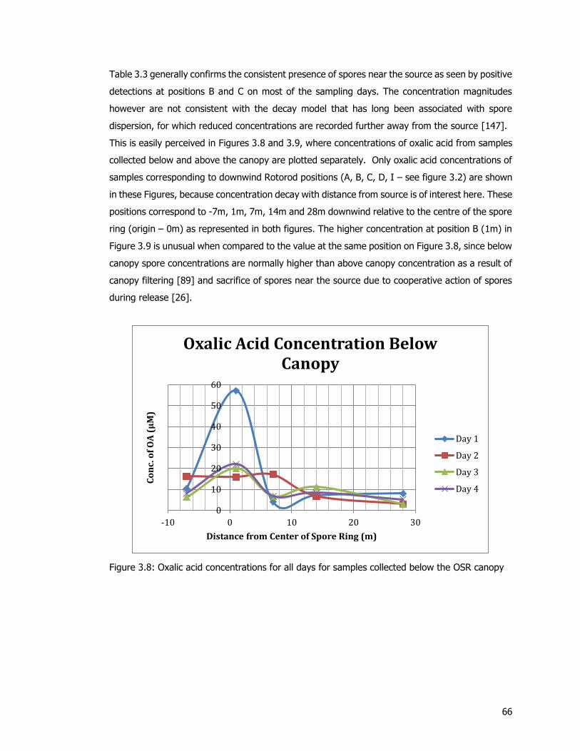


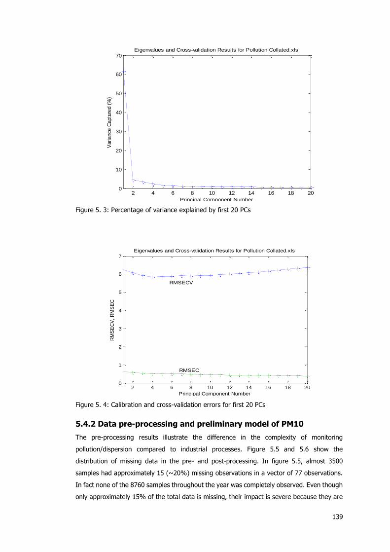


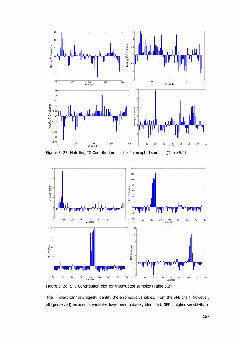


![Graphical modelling of multivariate time series · Graphical modelling of multivariate time series 237 Fig. 1 Encoding of relations XA XB [XX]by the a pairwise, b local, and c block-recursive](https://static.documents.pub/doc/80x56/5f9f3dbca39f3e3fad209cdf/graphical-modelling-of-multivariate-time-series-graphical-modelling-of-multivariate.jpg)