Modelling mass transfer in a rotating disk reaction vessel · In practice, a carbonate rock disk is...

Modelling mass transfer in a rotating disk reaction vessel KSG 2011

Modelling mass transfer in a rotating diskreaction vessel

Problem presented by

Frank Chang and Mustapha Abbad

Schlumberger Carbonate Research Dhahran

Executive Summary

A rotating disk apparatus is commonly used to study kinetics of heteroge-neous reactions such as calcite dissolution by acid. The apparatus consists ofa rock disk attached to a rotating shaft; the rock is submerged in a solutionof reactant which is transferred to the disk surface by convection and molec-ular diffusion. The former due to the rotation of the disk, and the latter dueto the concentration gradient of the reactant between the bulk fluid and therock surface.

Schlumberger is interested in determining how to use the rotating disk ex-periments to extract parameters that govern the reaction rate between theacid and carbonate rock. For mass transfer limited reactions these include(i) the diffusion rate across the boundary layer, and (ii) the thickness of theboundary layer. For a reaction that is surface limited, (i) the reaction rateand, (ii) the reaction order are of paramount interest.

The Study Group began by reanalyzing the solution by Levitch coupled withnumerical solutions of the flow in the hope that it would lead to a deeperunderstanding of the fluid dynamics in the neighbourhood of the rock. Inparticular, how the fluid flow changes as the Reynolds number is increasedand how this might indicate the most ideal location to measure the calciumin the reaction vessel.

The modelling looked not only at the coupling of the fluid flow with thediffusion equation for the ions but also a preliminary Stefan problem for thedissolving rock.

Version 1.0July 13, 2011iii+17 pages

I–i


Report coordinator

C. Sean Bohun

Contributors

C. Sean Bohun (University of Ontario Institute of Technology, Canada)Chris Breward (OCCAM, UK)

Mazen El-Ghoule (American University of Beirut, Lebanon)Luiz Faria (KAUST, Saudi Arabia)

Yiannis Hadjimichael (KAUST, Saudi Arabia)Nadeem Malik (KFUPM, Saudi Arabia)

John Norbury (OCIAM, UK)John Ockendon (University of Oxford, UK)

Xiang Sun (KAUST, Saudi Arabia)Jamal Uddin (University of Birmingham, UK)

Vladimir Zubkov (OCCAM, UK)

KSG 2011 was organised byKing Abdullah University of Science and Technology (KAUST)

In collaboration withOxford Centre for Collaborative Applied Mathematics (OCCAM)

I–ii


Contents

1 Introduction 11.1 Experimental setup . . . . . . . . . . . . . . . . . . . . . . . . . . . 11.2 Schematic of flow . . . . . . . . . . . . . . . . . . . . . . . . . . . . 2

2 Chemistry 42.1 The carbonic acid system . . . . . . . . . . . . . . . . . . . . . . . . 42.2 Solubility of calcium carbonate . . . . . . . . . . . . . . . . . . . . 6

3 Mathematical analysis 73.1 Strategy . . . . . . . . . . . . . . . . . . . . . . . . . . . . . . . . . 73.2 Velocity field preliminary analysis . . . . . . . . . . . . . . . . . . . 93.3 Von Karman similarity solutions . . . . . . . . . . . . . . . . . . . . 10

4 Reaction Rate 124.1 Concentration in the diffusive boundary layer . . . . . . . . . . . . 124.2 Finding the reaction rate . . . . . . . . . . . . . . . . . . . . . . . . 134.3 A Stefan problem for the Ca+ dissolution . . . . . . . . . . . . . . . 14

5 Summary 15

Bibliography 15

I–iii


1 Introduction

The rotating disk apparatus, as illustrated in Figure 1, is widely used in thepetroleum industry to study the kinetics of heterogeneous reactions such as in-terfacial calcium carbonate dissolution by acid. A review of the experimental use ofthis device can be found in [5]. The system allows for the determination of the re-action rate, the diffusion coefficient associated with the dissolution and the order ofthe reaction [1, 2, 3, 9]. In practice, a carbonate rock disk is attached to a rotatingshaft, and submerged in a solution of reactant (typically strong acid). The reactantis transferred to the rock surface by both convection and molecular diffusion withthe overall reaction rate governed by the slower of these two processes. Much ofthe theory is originally due to Levitch [4], with a refinement for a large Schmidt1

number [6], Sc, a few years later. One of the current difficulties is the significantvariability in the acid reaction rate data found in reservoir rocks which is attributedto a wide variation in experimental procedure [7, 8].

In [8] a few additional factors that could lead to variations in measured resultswere considered. (a) As the reaction progressed the apparent dissolution rate in-creases due to the increase in surface area. This effect is more likely when usingstrong acids or elevated temperatures. (b) Highly porous rocks will indicate a morerapid dissolution rate due to the increase in surface area but in this case the laminarflow assumed on the surface of the rock may no longer be valid. (c) Clay impuri-ties in the rock are capable of slowing the dissolution rate to as much as 25 times.Therefore some detailed mineralogy of the reservoir rock is required. (d) Acidizingadditives can also have a significant effect on the observed dissolution rate.

Some of the objectives that this report will address include: (i) an evaluationof the Reynolds number effects; (ii) determination of the motion of the fluid; (iii)consideration of the concentration profile and (iv) an indication of how to extractparameters that govern the reaction rate of the dissolution process.

1.1 Experimental setup

For the experiment detailed to the Study Group, a cylindrical pellet of calciumcarbonate rock, approximately 1/4 inch thick, was attached to a metal mount andsubmerged in the reaction vessel prior to the introduction of the reactant. A oneinch gap is maintained between the surface of the fluid and the top of the reactionvessel and a pressure of 1000 psi is maintained above the fluid to keep the gaseousby-products (carbon dioxide) in solution [3]. The reactant, 1 litre of 4.4 M HCl, isinjected over a period of about 30 seconds at a pressure of 3000 psi to create the1000 psi. This occurs while the rock is spun up to the desired speed. At this time,samples are taken every minute and the concentrations of both H+ and Ca2+ ionsare recorded. An example of the recorded data is shown in Figure 2.

The reactant reaching the (bottom) rock surface is consumed by chemical in-teraction, and Schlumberger are interested in quantifying the flux R (material per

1The Schmidt number Sc = µρD0

relates the relative thickness of the hydrodynamic layer andmass-transfer boundary layer.

I–1


Figure 1: Experimental setup showing (i) the pump that injects concentrated acid, (ii) therotating rock with shrink wrap exposing only the lower surface to the reactant and (iii) thesampling apparatus.

Figure 2: Experimental measurements of the hydrogen and calcium ion concentrations as afunction of time in seconds.

unit area per time) of this reaction which takes the form2 for a reaction order ofn = 1 of

R = 0.62D2/3ν−1/6ω1/2(cb − c0) (1)

where R is the flux from the disk surface, D is the diffusion coefficient of the solutein the solvent, ν = µ/ρ is the kinematic viscosity, ω is the angular velocity ofrotation and cb, c0 are the concentrations of solute in the bulk and at the disksurface respectively [4].

1.2 Schematic of flow

Measurements of the calcium concentration are taken soon after the acid is injected,without waiting for any possible transients in the ion concentrations to dissipate.In addition to this, samples from the reaction vessel were taken near the bottom ofthe reaction vessel against the outside wall where one would expect a recirculationcell in the fluid. Setting aside these issues, the motion of the fluid is driven by the

2For a general reaction order n, the industrial participant reports a generalized expression of

R = Φ(n)D2/3ν−1

3(1+n)R1−n

3(1+n)

d ω1

1+n (cb − c0) where Rd is the radius of the pellet and Φ(n) is aconstant dependent upon n.

I–2


Figure 3: Schematic of the expected flow streamlines and the induced circulation of calcium ions.However, in the actual apparatus the pipes for injection and sampling disturb the axisymmetryof the flow.

spinning action of the submerged disk and in response to this motion, fluid nearthe disk is thrown out to the sidewall. This flow will not be axisymmetric in theflow vessel shown in Figure 1.

There is an extensive body of literature dealing with the axisymmetric flowsproduced by spinning disks beginning with the work of von Karman [10] and con-tinuing to the present [11, 12, 13]. Since the disk is submerged and is some distancefrom the sidewalls of the reaction vessel, it is not clear if there is a steady solutionin the time frame of the experiment (5 minutes, sampling every 1 minute). Indeed,measurements in the lab have shown that occasionally [Ca2+] decreases with time.This may be due to the location of where the [Ca2+] is sampled. Currently this isat the bottom of the reaction vessel adjacent to the outside wall where one mightexpect a circulation cell in the flow. If the sampling point is within such a cellthen the measurement will not be a true determination of what is occurring at thedissolution front. One of the questions that should be considered is to identify thebest point to sample [Ca2+].

Inside the reaction vessel the apparatus for sampling the fluid and injecting thereactant may complicate the structure of the flow. However, all that matters fordissolving the rock is the availability of H+ ions through the reaction

2H+ + CaCO3(s) Ca2+ + CO2(g) + H2O.

If the limiting step in the dissolution is mass transfer from the rock into the solution,or the supply of hydrogen ions from the solution to the rock, then increasing therotation speed ω would increase this mass transfer and increase the overall reactionrate. On the other hand, if the mass transfer rate exceeds the rock consumption ratethen the dissolution becomes surface-reaction limited and the overall reaction ratethen becomes independent of ω giving a schematic behaviour as shown in Figure 4.

A final point of concern is the effect of the bounding shrink wrap on the rockpellet. As the rock erodes, the boundary layer can become trapped by the nonre-active lip at the edge of the disk. This has the possibility of significantly changingthe dynamics of the dissolution in the later stages of an experiment.

I–3


Figure 4: Schematic of the reaction rate as a function of the disk rotation speed.

2 Chemistry

2.1 The carbonic acid system

As the calcium carbonate is eaten away from the rock it injects carbonate ionsinto solution which react with the carbonate already present in solution due to thehigh pressure dissolving carbon dioxide into the solution. It is helpful to carefullyquantify this chemistry before a more ambitious model is attempted.

We begin with the basic carbonic acid system where CO2(g) dissolves in waterto its aqueous form CO2(aq) and the subsequent formation of carbonic acid. Thecarbonic acid decomposes into bicarbonate HCO−3 (aq) and carbonate CO2−

3 (aq) ionsdepending upon the pH of the solution. The equilibrium system is the following

CO2(g) + H2O CO2(aq) + H2O, K0 =[CO2(tot)]

P (CO2), (2a)

H2CO3(aq) � H+(aq) + HCO−3 (aq), Ka1 =[H+][HCO−3 ]

[CO2(tot)], (2b)

HCO−3 (aq) � H+(aq) + CO2−3 (aq), Ka2 =

[H+][CO2−3 ]

[HCO−3 ], (2c)

H2O � H+(aq) + OH−(aq), Kw = [H+][OH−], (2d)

where the notation [·] denotes the concentration of a particular quantity in moles/litreand P (·) denotes the partial pressure measured in atmospheres. The quantity[CO2(tot)] denotes the concentration of the total amount of dissolved carbon diox-ide which contains a small3 admixture of dissolved carbonic acid. Values of the

3Carbonic acid produced with the reaction CO2(aq) + H2O H2CO3(aq) satisfies [H2CO3] =Kh[CO2] where lnKh = −7.49 + 219/T . At 25o C only a small portion is converted [H2CO3] =1.16× 10−3[CO2].

I–4


disassociation constants are temperature dependent and given by

log10K0 = 2622.38/T + 0.0178471T − 15.5873, (3a)

log10Ka1 = −3404.71/T − 0.032786T + 14.8435, (3b)

log10Ka2 = −2902.39/T − 0.02379T + 6.4980, (3c)

lnKw = 148.9802− 13847.26/T − 23.6521 lnT, (3d)

where T is the absolute temperature [14, 15, 16, 18].Along with these reactions are expressions for both charge and mass balance.

For charge balance, one ensures that∑

i zici = 0 where zi and ci are respectivelythe charge and concentration of species i. This reduces to the constraint that

[H+]− 2[CO2−3 ]− [HCO−3 ]− [OH−] = 0. (4)

For the mass balance, the total dissolved inorganic carbon

F1 = [CO2(tot)] + [HCO−3 ] + [CO2−3 ] (5)

is constant.By combining Ka1 and Ka2 and using (5) one can determine the fractional

amounts of the acid as a function of [H+]

α0 =1

F1

[CO2(tot)] =[H+]2

[H+]2 +Ka1[H+] +Ka1Ka2

, (6a)

α1 =1

F1

[HCO−3 ] =Ka1[H+]

[H+]2 +Ka1[H+] +Ka1Ka2

, (6b)

α2 =1

F1

[CO2−3 ] =

Ka1Ka2

[H+]2 +Ka1[H+] +Ka1Ka2

. (6c)

To solve for [H+] as a function of P (CO2), expression (2) is taken with (4) to findthat

[H+]3 − (K0Ka1P (CO2) +Kw)[H+]− 2K0Ka1Ka2P (CO2) = 0. (7)

Figure 5 shows the concentration of H+, the solution to (7), as a function of thepartial pressure of carbon dioxide. The black circle corresponding to an air pressureof 1 atm. At this air pressure the partial pressure of CO2 is P (CO2) = 39 Pa orabout 3.85×10−4 atm giving [H+] = 2.41×10−6 M (pH = 5.62). Equation (6) yieldsα0 = 0.844, α1 = 0.156 and α2 = 3.0×10−6 for [CO2(aq)] = 1.54×10−5 M, [HCO−3 ] =2.41 × 10−6 M and [CO2−

3 ] = 4.67 × 10−11 M. These values are reflected with theblack circles in Figure 6. The squares in Figures 5, 6 correspond to an atmosphericpressure of 1000 psi or roughly 68 atm. In this case, [H+] = 1.99 × 10−5 M (pH =4.70), α0 = 0.978, α1 = 0.022, α2 = 5.2 × 10−8, [CO2(aq)] = 9.06 × 10−4 M,[HCO−3 ] = 1.99× 10−5 M and [CO2−

3 ] = 4.68× 10−11 M. As P (CO2) → ∞, [H+] →(K0Ka1P (CO2))1/2 and as a result [CO2−

3 ]→ Ka2.

I–5


10−8 10−6 10−4 10−2 100 1023

3.5

4

4.5

5

5.5

6

6.5

7

P(CO2) (atm)

pH

T = 25o C

T = 50o C

Figure 5: The dependence of the pH of a sample of pure water as a function of the applied partialpressure of carbon dioxide gas. Increasing the temperature decreases the pH at low pressures dueto the change in Kw. At high pressures, pH ∼ 1

2 logP . The circle corresponds to an atmosphericpressure of 1 atm and the square corresponds to 1000 psi (∼ 68 atm).

0 2 4 6 8 10 12 140

0.1

0.2

0.3

0.4

0.5

0.6

0.7

0.8

0.9

1

pH

Frac

tiona

l com

pone

nt

[CO2(tot)]

[HCO3−]

[CO32−]

Figure 6: Fractional components of the acidic species of carbonic acid as a function of the pH ofthe solution at 25oC. Circles correspond to a pressure of 1 atm (pH = 5.62) and squares correspondto 1000 psi (∼ 68 atm) (pH = 4.70).

2.2 Solubility of calcium carbonate

In the presence of carbonate rock, the solubility depends on the amount of dissolvedinorganic carbon in the water due to the applied pressure. We include the reaction

CaCO3(s) Ca2+(aq) + CO2−3 (aq), Ksp = [Ca2+][CO2−

3 ] (8a)

where

log10Ksp = −171.9065− 0.077993T + 2839.319/T − 71.595 log10 T (8b)

I–6


due to Mucci [19]. The charge balance expression becomes

2[Ca2+] + [H+]− 2[CO2−3 ]− [HCO−3 ]− [OH−] = 0. (9)

and continuing as we did in the case of just carbonic acid, [H+] satisfies

[H+]3 − (K0Ka1P (CO2) +Kw)[H+]

−2K0Ka1Ka2P (CO2) =2Ksp[H

+]4

K0Ka1Ka2P (CO2)

(10)

which should be compared to (7).It is interesting to notice what happens to the solution of (10) as P (CO2) varies.

At 1 atm (P (CO2) = 3.85×10−4 atm) we find the equilibrium [H+] = 1.57×10−7 M(pH = 6.80), [CO2(aq)] = 1.30× 10−5 M, [HCO−3 ] = 3.70× 10−5 M, [CO2−

3 ] = 1.11×10−8 M, and [Ca2+] = 4.50× 10−1 M. Increasing to 1000 psi (∼ 68 atm) (P (CO2) =2.62 × 10−2 atm), [H+] = 1.29 × 10−6 M (pH = 5.89), [CO2(aq)] = 8.86 × 10−4 M,[HCO−3 ] = 3.06×10−4 M, [CO2−

3 ] = 1.11×10−8 M, and [Ca2+] = 4.49×10−1 M. Eventhough there is nearly 68 times the dissolved carbon in solution, the equilibriumamount of carbonate ion is virtually the same due to the buffering action of thebicarbonate ion.

In our case, the pH is controlled in that 1 litre of 4.4 M HCl is injected intothe reaction vessel and if x moles of CaCO3 dissolves, then x moles of Ca2+ and xmoles of CO2−

3 are formed. The carbonate ions that are ejected into the solutionwill be distributed amongst the different acid forms but since we know the pH,we know that the proportion that remains as carbonate is given by α2. That is,Ksp = [Ca2+][CO2−

3 ] = α2x2 or alternatively the molar solubility is given by

[Ca2+] =

(Ksp

α2([H+])

)1/2

=

(Ksp

Ka1Ka2

)1/2 ([H+]2 +Ka1[H+] +Ka1Ka2

)1/2.

At 25o C, a solution of 4.4 M HCl results in a massive molar solubility of CaCO3(s)of 6.8× 104 M.

3 Mathematical analysis

3.1 Strategy

The Study group is primarily interested in the dissolution of a carbonate rock ina rotating disk apparatus. From Section 2 it can be seen that the dissolution rateof CaCO3(s) depends on the availability of H+, and in a well mixed solution, theenvironment of the apparatus is chosen so that Ca2+ solubility is enhanced and theformation of CO2 gas is suppressed. Note that the generation of CO2 in the form ofbubbles rather than in an aqueous form, can change the nature of the fluid flow.

Because the flow field is generated by a spinning disk at one end of the appara-tus, it is natural to assume that, provided the flow is laminar, it will have the formof a von Karman similarity solution. However, there are some significant differences

I–7


Description Symbol Value

Depth of the top of the rotating mount L0 1.5× 10−2 mDepth of the rock face Ld 3.0× 10−2 mTotal depth of the reaction vessel Lc 2.3× 10−1 mRadius of the reaction vessel Rc 7.5× 10−2 mRadius of the rock Rd 1.905× 10−2 mRotational speed ω 200− 1000 rpmDensity of the fluid ρ 1× 103 kg m−3

Viscosity of the fluid µ 1× 10−3 Pa sDiffusion coefficient of Ca2+ D0 7.1× 10−10 m2 s−1

Schmidt number Sc 1.41× 103

Table 1: The physical parameters for the reaction vessel, the fluid flow and the dissolution ofCa2+ ions.

between our situation and that of the classical von Karman case. Namely, the spin-ning disk does not completely cover the top of the reaction vessel and moreover, itis submerged so there is the possibility that an additional circulation cell could formabove the disk, changing the nature of the flow. These differences are significantenough to justify a preliminary analysis of the flow field using a CFD program. Forour purposes, we chose the package COMSOL based on its availability. Once thefluid velocity is resolved, it can be coupled to an advection-diffusion equation todescribe the dissolving Ca2+ ions and from that, the flux of material leaving thecarbonate rock.

Figure 7 illustrates the geometry of the idealized apparatus, with the inlet/outletpipes omitted, so that axisymmetric flow is possible and Table 1 lists physicalvalues4.

Figure 7: Geometry and boundary conditions for the fluid flow within the idealized reactionvessel.

4The value of D0 comes from [17].

I–8


3.2 Velocity field preliminary analysis

The group considered an axisymmetric model for the flow in cylindrical coordinateswith the origin located at the disk, the positive direction towards the bottom of thereaction vessel. The fluid flow is assumed to be incompressible and described bythe steady state Navier-Stokes equation. It is driven by the motion of the rock andthen coupled with an advection-diffusion equation for the transport of Ca2+ ions.

In detail, the fluid velocity ~u(r, z) = (ur(r, z), uθ(r, z), uz(r, z)), satisfies

ur∂ur∂r− u2

θ

r+ uz

∂ur∂z

=µ

ρ

(1

r

∂

∂r

(r∂ur∂r

)− urr2

+∂2ur∂z2

), (11a)

ur∂uθ∂r

+uθurr

+ uz∂uθ∂z

=µ

ρ

(1

r

∂

∂r

(r∂uθ∂r

)− uθr2

+∂2uθ∂z2

), (11b)

ur∂uz∂r

+ uz∂uz∂z

= −1

ρ

∂P

∂z+µ

ρ

(1

r

∂

∂r

(r∂uz∂r

)+∂2uz∂z2

), (11c)

where the pressure P = P (z) is assumed to depend only on the depth and with theincompressibility condition

1

r

∂

∂r(rur) +

∂uz∂z

= 0. (12)

The free surface condition at z = −Ld is assumed to be stress free and all internalsurfaces are taken to have a no-slip condition

∂uz∂z

= 0,∂uθ∂z

= 0, uz = 0; z = −Ld, (13a)

~u = ~0; z = Lc − Ld, (13b)

~u = ~0; r = Rc, (13c)

~u = (0, ωr, 0); z = 0,−|Ld − L0|, 0 < r < Rd, (13d)

~u = (0, ωRd, 0); r = Rd, −|Ld − L0| < z < 0. (13e)

Results for the velocity field for ω = 50, 100, 200 rad/s (477 − 1910 rpm) aredepicted in Figure 8. Note that the axis of symmetry is on the left edge of eachplot and that the aspect ratio is not preserved. The existence of the isolated vortexnear the wall suggests that sampling near the bottom may lead to fluctuations inmeasured [Ca2+]. The wall opposite the rotating disk might be a better position tosample the fluid. The structure of the flow has many of the same features of thevon Karman similarity solution despite the fact that the disk is of finite extent andsubmerged within the fluid.

The thickness of the hydrodynamic or viscous boundary layer under the disk canbe estimated by solving for the velocity of the Ekman layer. In a neighbourhood ofz = 0 this takes the form in cylindrical coordinates of ~u(z) = u0e

−λz(sinλz, cosλz, 0)where λ2 = ρω/2µ. The thickness δ is defined as that depth where ~u(δ)/|~u(δ)| =−~u(0)/|~u(0)| or λδ = π so that

δ = π

(2µ

ρω

)1/2

.

I–9


ω = 50 rad/s ω = 100 rad/s

ω = 200 rad/s ω = 200 rad/s

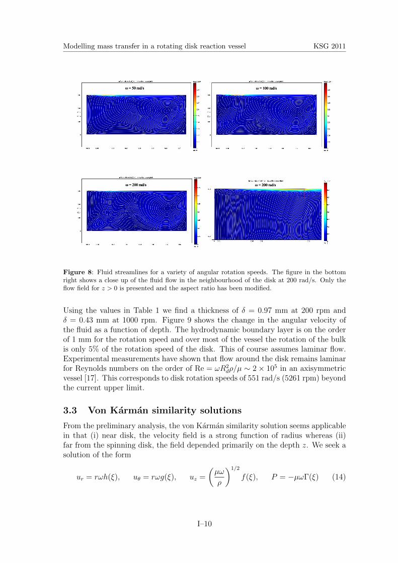
Figure 8: Fluid streamlines for a variety of angular rotation speeds. The figure in the bottomright shows a close up of the fluid flow in the neighbourhood of the disk at 200 rad/s. Only theflow field for z > 0 is presented and the aspect ratio has been modified.

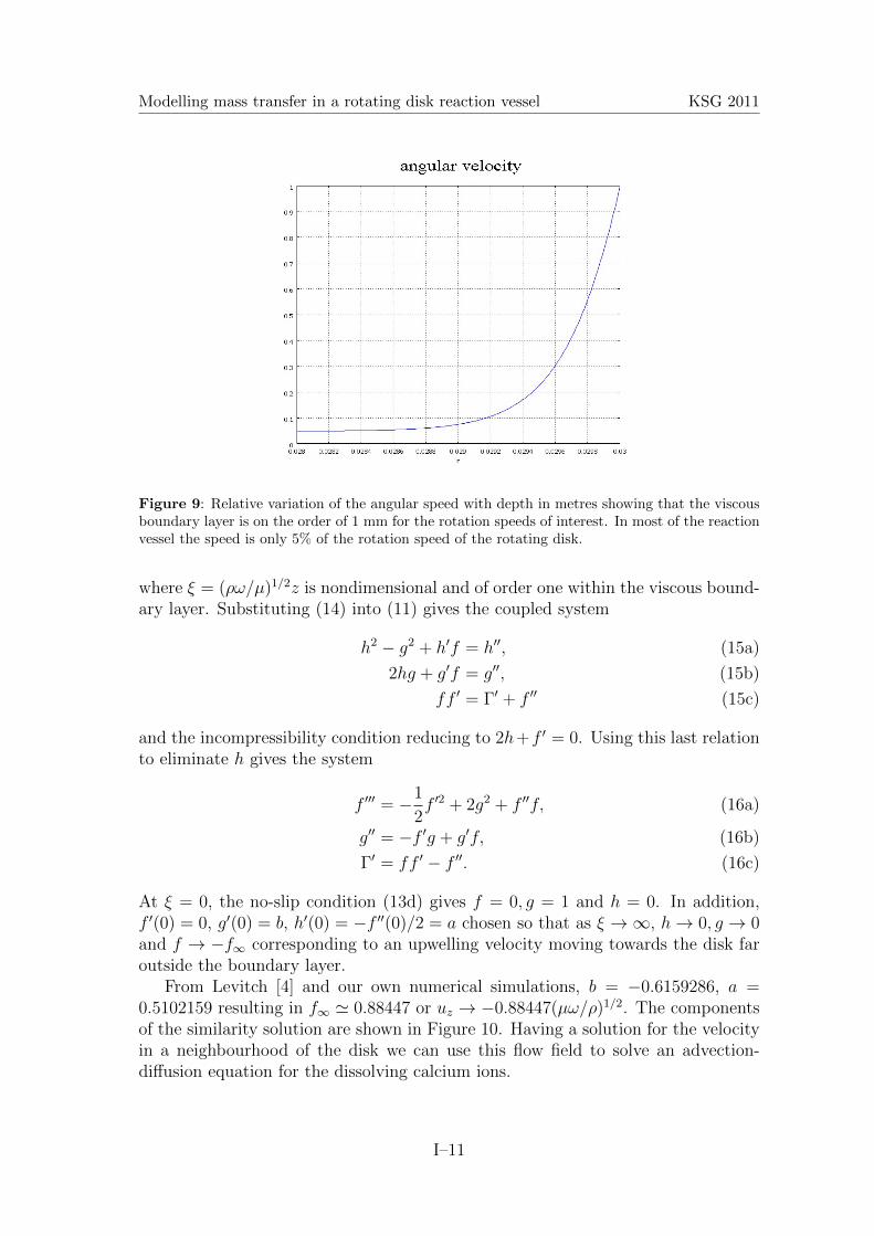
Using the values in Table 1 we find a thickness of δ = 0.97 mm at 200 rpm andδ = 0.43 mm at 1000 rpm. Figure 9 shows the change in the angular velocity ofthe fluid as a function of depth. The hydrodynamic boundary layer is on the orderof 1 mm for the rotation speed and over most of the vessel the rotation of the bulkis only 5% of the rotation speed of the disk. This of course assumes laminar flow.Experimental measurements have shown that flow around the disk remains laminarfor Reynolds numbers on the order of Re = ωR2

dρ/µ ∼ 2× 105 in an axisymmetricvessel [17]. This corresponds to disk rotation speeds of 551 rad/s (5261 rpm) beyondthe current upper limit.

3.3 Von Karman similarity solutions

From the preliminary analysis, the von Karman similarity solution seems applicablein that (i) near disk, the velocity field is a strong function of radius whereas (ii)far from the spinning disk, the field depended primarily on the depth z. We seek asolution of the form

ur = rωh(ξ), uθ = rωg(ξ), uz =

(µω

ρ

)1/2

f(ξ), P = −µωΓ(ξ) (14)

I–10


Figure 9: Relative variation of the angular speed with depth in metres showing that the viscousboundary layer is on the order of 1 mm for the rotation speeds of interest. In most of the reactionvessel the speed is only 5% of the rotation speed of the rotating disk.

where ξ = (ρω/µ)1/2z is nondimensional and of order one within the viscous bound-ary layer. Substituting (14) into (11) gives the coupled system

h2 − g2 + h′f = h′′, (15a)

2hg + g′f = g′′, (15b)

ff ′ = Γ′ + f ′′ (15c)

and the incompressibility condition reducing to 2h+f ′ = 0. Using this last relationto eliminate h gives the system

f ′′′ = −1

2f ′2 + 2g2 + f ′′f, (16a)

g′′ = −f ′g + g′f, (16b)

Γ′ = ff ′ − f ′′. (16c)

At ξ = 0, the no-slip condition (13d) gives f = 0, g = 1 and h = 0. In addition,f ′(0) = 0, g′(0) = b, h′(0) = −f ′′(0)/2 = a chosen so that as ξ →∞, h→ 0, g → 0and f → −f∞ corresponding to an upwelling velocity moving towards the disk faroutside the boundary layer.

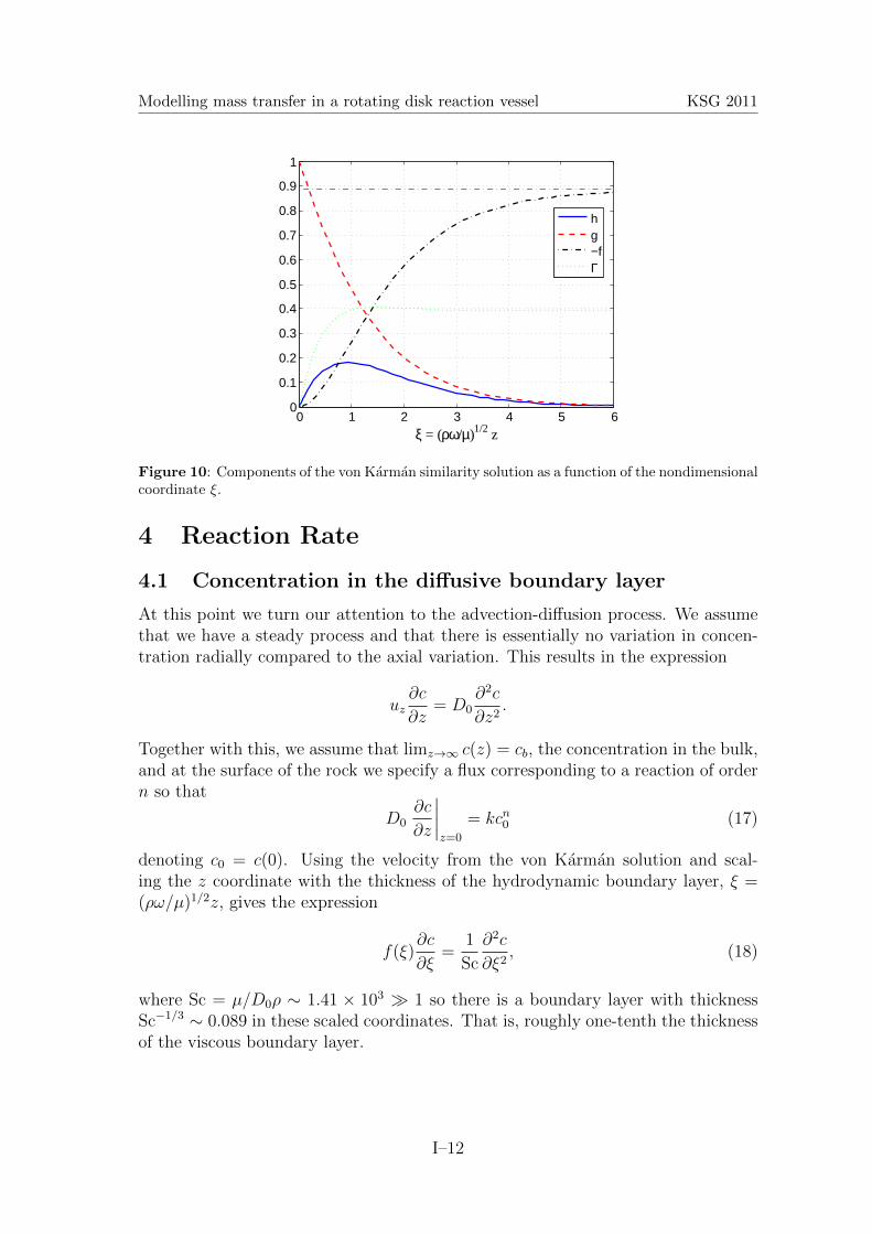
From Levitch [4] and our own numerical simulations, b = −0.6159286, a =0.5102159 resulting in f∞ ' 0.88447 or uz → −0.88447(µω/ρ)1/2. The componentsof the similarity solution are shown in Figure 10. Having a solution for the velocityin a neighbourhood of the disk we can use this flow field to solve an advection-diffusion equation for the dissolving calcium ions.

I–11


0 1 2 3 4 5 60

0.1

0.2

0.3

0.4

0.5

0.6

0.7

0.8

0.9

1

ξ = (ρω/µ)1/2 z

hg−fΓ

Figure 10: Components of the von Karman similarity solution as a function of the nondimensionalcoordinate ξ.

4 Reaction Rate

4.1 Concentration in the diffusive boundary layer

At this point we turn our attention to the advection-diffusion process. We assumethat we have a steady process and that there is essentially no variation in concen-tration radially compared to the axial variation. This results in the expression

uz∂c

∂z= D0

∂2c

∂z2.

Together with this, we assume that limz→∞ c(z) = cb, the concentration in the bulk,and at the surface of the rock we specify a flux corresponding to a reaction of ordern so that

D0∂c

∂z

∣∣∣∣z=0

= kcn0 (17)

denoting c0 = c(0). Using the velocity from the von Karman solution and scal-ing the z coordinate with the thickness of the hydrodynamic boundary layer, ξ =(ρω/µ)1/2z, gives the expression

f(ξ)∂c

∂ξ=

1

Sc

∂2c

∂ξ2, (18)

where Sc = µ/D0ρ ∼ 1.41 × 103 � 1 so there is a boundary layer with thicknessSc−1/3 ∼ 0.089 in these scaled coordinates. That is, roughly one-tenth the thicknessof the viscous boundary layer.

I–12


Solving (18) and applying the boundary condition as ξ →∞ gives

c(ξ) = c0 + (cb − c0)

∫ ξ

0

e∫ t Sc f(s) dsdt∫ ∞

0

e∫ t Sc f(s) dsdt

(19)

with c0 chosen to satisfy the flux condition (17) at the surface.

4.2 Finding the reaction rate

Having determined the concentration, the rate at which material leaves the rock isthe integrated flux over the dissolving surface. Since we have assumed no radialdependence, one has

πR2dR =

∫∫disk

D0∂c

∂z

∣∣∣∣z=0

dA = πkR2dcn0 (20a)

with

cn0

∫ ∞0

e∫ t Sc f(s) dsdt =

D0

k

(ρω

µ

)1/2

(cb − c0). (20b)

Traditionally one estimates the integral by replacing f(ξ) with the first term of itsTaylor series [4], f(ξ) ∼ −aξ2 +O(ξ3) and finds

I∞(Sc) =

∫ ∞0

e∫ t Sc f(s) dsdt ∼

(a Sc

3

)−1/3∫ ∞0

e−t3

dt =

(a Sc

3

)−1/3

Γ

(4

3

). (21)

Alternatively, if one is already solving the system (15) then

I∞(Sc) = limx→∞

I(x; Sc)

where I(x; Sc) satisfies I ′′ = Sc f(x)I ′; I(0) = 0, I ′(0) = 1. Using this technique wefind

I∞(Sc) ' ASc−γ (22)

where A = 2.08938, γ = 0.35469. A comparison of these estimates is shown inFigure 11.

At this point one could solve R as a function of n numerically. Specializing tothe case of n = 1, equation (20b) gives the approximation

c0 = cb

((a1/3

31/3Γ(4/3)

)−1

kD−2/30

(µ

ρ

)1/6

ω−1/2 + 1

)−1

leading to the asymptotic expression with respect to ω of

R = cb

a1/3

31/3Γ(4/3)D

2/30

(µρ

)−1/6

ω1/2, ω → 0,

k, ω →∞.(23)

I–13


0 1 2 3 4 5 6 7−2.5

−2

−1.5

−1

−0.5

0

0.5

log10

Sc

log 10

I ∞(S

c)

Figure 11: Comparison of the various estimates of I∞(Sc). The circles are the actual data points,the solid line is the estimate (22) and the dashed line is the traditional estimate (21).

If expression (22) is used instead then one has

R = cb

A−1D1−γ0

(µρ

)γ−1/2

ω1/2, ω → 0,

k, ω →∞.(24)

Returning to the traditional estimate, noting that a1/3

31/3Γ(4/3)= 0.62044, we see

that we have reproduced the original expression (1) given back in Section 1. Alsoof interest is the case when c0 � cb. In this regime,

R = kcn0 ∼a1/3

31/3Γ(4/3)D

2/30

(µ

ρ

)−1/6

ω1/2cb

for any order n in contradiction to the expression suggested by Schlumberger.

4.3 A Stefan problem for the Ca+ dissolution

A simple Stefan problem has been proposed to predict the rate at which calciumcarbonate is being dissolved and hopefully to explain the swirling patterns we ob-served. In this first iteration we ignore the velocity field and assume only diffusionin the bulk. A one dimensional model was taken and assumes that the rock extendsfrom z = 0 to z = S(t) with S(0) = S0 being the initial thickness. The solidhas some intrinsic concentration which decreases as it is dissolved into the solutionand the rate at which this material is lost is taken up in motion of the dissolvinginterface. The speed of the interface is related to the jump in concentration at thesurface. As mentioned, in the bulk of vessel S(t) < z < L, the concentration sat-isfies the diffusion equation (ignoring advection) and a no flux boundary conditionis specified at the bottom of the vessel at z = L.

I–14


Putting all these assumptions together gives the model

c(z, t) = cs; 0 ≤ z < S(t), t ∈ (0, T ]

∂c

∂t= D

∂2c

∂z2; S(t) < z < L, t ∈ (0, T ]

∂c

∂z= 0; z = L, t ∈ (0, T ];

c(z, t) = c0; z = S(t), t ∈ (0, T ]

(cs − c0)dS

dt= D

∂c

∂z; z = S(t), t ∈ (0, T ], S(0) = S0

where cs is the concentration of the solid rock and initially we assume some bulkconcentration in the solution c(z, 0) = cb for S0 < z < L. T is defined as that timewhere S(T ) = 0 and all the material has dissolved. To validate this model it shouldpredict the observed dissolution rate of dS/dt ∼ 3/5 mm per minute (10−5 m s−1).

5 Summary

The flow within the experimental apparatus was modelled and it was found thatthe Reynolds number varies significantly from the bulk to the layer near the edgeof the rotating disk with values from 1000-5000 but the onset of turbulence isnot expected until a rotation speed of roughly 5200 rpm. Using COMSOL, theflow was shown to be axisymmetric but in reality it may be more complicatedwith time dependent behaviour in the corners of the reaction vessel and near thedisk. This behaviour will modify the transport of the Ca2+ ions which suggeststhat a better place to sample the concentration would be away from thebottom of the reaction vessel near the side wall opposite the rotatingdisk. One concern is the edge of the disk which was assumed to erode in themodelling described herein. By having material on the edge which does not erode,there is the possibility that a high concentration of ions could be trapped near thesurface of the disk, artificially slowing its dissolution. It was proposed that using amaterial that dissolved might lead to an improvement in the results. The literatureon the kinetics of the dissolution of carbonate could be coupled into the model toproduce profiles of the concentration of the various chemical species. Details of thisnature have so far ignored the advection of the fluid. Another avenue of interestmight be to include the porosity of the rock in the Stefan model that was proposed.

Bibliography

[1] Lund, K. et al. (1973). Acidization I. The Dissolution of Dolomite in Hydrochlo-ric Acid. Chemical Engineering Science, 28, pp. 691-700.

[2] Lund, K. et al. (1975). Acidization II. The Dissolution of Calcite in Hydrochlo-ric Acid. Chemical Engineering Science, 30, pp. 825-835.

I–15


[3] Fredd, C.N. & Fogler, H.S. (1998). The Kinetics of Calcite Dissolution in AceticAcid Solutions. Chemical Engineering Science, 53(22), pp. 3863-3874.

[4] Levitch, V.G. (1962). Physicochemical Hydrodynamics, Prentice-Hall Inc., En-glewood Cliffs, N.J.

[5] Boomer, D.R. et al. (1972). Rotating Disk Apparatus for Reaction Rate Studiesin Corrosive Liquid Environments. The Review of Scientific Instruments, 43(2),pp. 225-229.

[6] Newman, J. (1966). Schmidt Number Corrections for the Rotating Disk. Journalof Physical Chemistry, 70(4), pp. 1327-1328.

[7] Taylor, K.C. et al. (2004). Measurement of Acid Reaction Rates of a DeepDolomitic Gas Reservoir. Journal of Canadian Petroleum Technology, 43(10),pp. 49-56.

[8] Taylor, K.C. & Nasr-El-Din, H.A. (2009). Measurement of Acid Reaction Rateswith a Rotating Disk Apparatus. Journal of Canadian Petroleum Technology,48(6), pp. 66-70.

[9] Prakongpan, S. et al. (1976). Dissolution Rate Studies of Cholesterol Monohy-drate in Bile Acid-Lecithin Solutions Using the Rotating-Disk Method. Journalof Pharmaceutical Sciences, 65(5), pp. 685-689.

[10] Karman, T. von. (1921). Uber laminare und turbulente Reibung. Zeitschrift furAngewandte Mathematik und Mechanik (ZAMM), 1(4), pp. 233-252

[11] Escudier, M.P. (1984). Observations of the flow produced in a cylindrical con-tainer by a rotating endwall. Experiments in Fluids, 2, pp. 189-196.

[12] Brady, J.F. & Durlofsky, L. (1987). On rotating disk flow. Journal of FluidMechanics, 175, pp. 363-394.

[13] Hyun, J.M. & Kim, J.W. (1987). Flow driven by a shrouded spinning disk withaxial suction and radial inflow. Fluid Dynamics Research, 2, pp. 175-182.

[14] Harned, H.S., & Davis, R.D. (1943). The ionization constant of carbonic acidin water and the solubility of carbon dioxide in water and aqueous salt solutionsfrom 0 to 50o C. Journal of the American Chemical Society, 65(10), pp. 2030-2037.

[15] Harned, H.S., & Scholes, S.R. (1941). The ionization constant of HCO−3 from0 to 50o C. Journal of the American Chemical Society, 63(6), pp. 1706-1709.

[16] Dickson, A.G. & Riley, J.P. (1979). The estimation of acid dissociation con-stants in seawater media from potentionmetric titrations with strong base. I.The ionic product of water - Kw. Marine Chemistry, 7(2), pp. 89-99.

I–16


[17] Liu, Z. & Dreybrod, W. (1997). Dissolution kinetics of calcium carbonate min-erals in H2O−CO2 solutions in turbulent flow: The role of the diffusion bound-ary layer and the slow reaction H2O+ → H+ + HCO−3 . Geochimica et Cos-mochimica Acta, 61(14), pp. 2879-2889.

[18] Soli, A.L. & Byrne, R.H. (2002). CO2 system hydration and dehydration ki-netics and the equilibrium CO2/H2CO3 ratio in aqueous NaCl solution. MarineChemistry, 78(2-3), pp. 65-73.

[19] Mucci, A. (1983). The solubility of calcite and aragonite in seawater at varioussalinities, temperatures and one atmosphere total pressure. American Journalof Science, 283, pp. 780-799.

I–17

Date post:	01-May-2018
Category:	Documents
Upload:	dolien
View:	216 times
Download:	0 times

Modelling mass transfer in a rotating disk reaction vessel · In practice, a carbonate rock disk is...

Documents