IMPERIAL COLLEGE OF SCIENCE, TECHNOLOGY AND MEDICINE UNIVERSITY OF LONDON MODELLING OF ULTRASONIC GUIDED WAVE FIELD GENERATED BY PIEZOELECTRIC TRANSDUCERS by Pierre Noël Marty A thesis submitted to the University of London for the degree of Doctor of Philosophy Department of Mechanical Engineering Imperial College of Science, Technology and Medicine London SW7 2BX March 2002
Transcript
IMPERIAL COLLEGE OF SCIENCE, TECHNOLOGY AND MEDICINE
UNIVERSITY OF LONDON
MODELLING OF ULTRASONIC GUIDED WAVEFIELD GENERATED BY PIEZOELECTRIC
TRANSDUCERS
by
Pierre Noël Marty
A thesis submitted to the University of London for the degree of
Doctor of Philosophy
Department of Mechanical EngineeringImperial College of Science, Technology and Medicine
London SW7 2BX
March 2002
Dedication
To my dad
Steganographia, hoc est ars per occultam scrituramanimi sui voluntanen absentibus aperiendi certa
Thritème
Francfort, 1606
Acknowledgements
I wish to sincerely express my thanks to Prof. Peter Cawley, Dr. Mike Lowe,and Denis Hitchings who have provided invaluable guidance, technical knowledge,support and linguistic advice throughout this project. I would also like to thank Prof.Bert Auld for his help during his two visits to Imperial College. He took a large part inthe guidance of the project and enlightened it with his invaluable advice.
Welcome advice, discussions and ideas, in various forms, were often providedby other members of the non-destructive testing group at Imperial College. I enjoyedmy time amongst you. They are, in approximately the order of appearance, DavidAlleyne, Andrew Chan, Mark Evans, Richard Monkhouse, Keith Vine, Brent Zeller,Brian Pavlakovic, Paul Wilcox, Michel Castaings, Arnaud Bernard, Rob Long, RogerDalton, Christophe Aristégui, Stephane Baly, Jon Allen, Malcom Beard, Thomas Vogt,Alexandro Demma, Francesco Simonetti, Grzegorz Grondek and Richard Sepping.
I must thank the EPSRC and the NDT group for their financial support.
My best thanks are due to my family (you Michèle and Dominique) and Nina fortheir help, support and understanding during all the time I spent far from them. Nina,my warmest thanks for your enthusiasm, your confidence, and your love.
Abstract
The thesis investigates some aspects of the fundamental science necessary forthe development of piezoelectric sensors for use in integral structural inspection systemsbased on ultrasonic Lamb waves. It is particularly concerned with the analysis of theelectromechanical interaction, the process of generation of Lamb wave modes and thedesign of permanently attached transducers such as PVDF-based interdigital transducers(IDT) or ceramic-based piezoelectric strips.
Interdigital transducers developed for use in smart structures are now at thestage where practical applications on plate and pipe structures are being considered. Forsuch a transducer to be used, it is necessary to understand exactly the electromechanicalinteraction and the internal scattering phenomena governing their performance. Ananalytical investigation into the interactions that occur between mechanical fields andelectric quantities is presented. This model is developed for a simple transducer design,a single-strip transducer under plane strain conditions. A computer model for predictingthe acoustic field generated by a given voltage applied to the transducer and vice-versais presented. This model is developed on the basis of normal mode theory andperturbation methods, providing flexibility and physical insight. Intermediatecalculations as well as final results are validated using the finite element modeldeveloped in parallel with this work. Since the analytical model is based on assumptionsmainly related to the perturbation methods, these are discussed and limits of the modelas well as its eventual extensions are drawn.
The thesis is also concerned with a numerical analysis based on the finiteelement method. A finite element formulation that includes the piezoelectric orelectroelastic effect alongside the dynamic matrix equation of electroelasticity and itsreduction to the well-known equation of structural dynamics, based on a strong analogybetween electric and elastic variables, is presented. It is shown how these equationswere incorporated in an already existing finite element code. In parallel with validation,results are produced to identify several important features that are not taken into accountin the analytic model. Results are presented for IDTs and checked against experimentaldata when measuring displacement field amplitudes using a laser probe.
Page I
Contents
MODELLING OF ULTRASONIC GUIDED WAVE FIELD GENERATED BYPIEZOELECTRIC TRANSDUCERS ......................................................................................................1
1.1 ADVANTAGES OF LAMB WAVES INSPECTION TECHNIQUES ..........................................................181.2 PERMANENTLY ATTACHED TRANSDUCER TECHNOLOGY FOR SMART STRUCTURES .....................181.3 MODELLING OF FIELD GENERATED BY PIEZOELECTRIC TRANSDUCERS........................................19
1.3.1 Finite Element Analysis......................................................................................................201.3.2 Analytical Model ................................................................................................................21
2.1 PLATE WAVES...............................................................................................................................282.1.1 Propagation in Unbounded Nedia.......................................................................................292.1.2 The Law of Refraction of Plane Waves at an Interface ......................................................342.1.3 Lamb Waves .......................................................................................................................34
CHAPTER 3 FINITE ELEMENT MODELLING OF PIEZOELECTRICITY................................51
3.1 INTRODUCTION .............................................................................................................................523.2 ADDITION OF THE PIEZOELECTRIC EQUATIONS.............................................................................53
3.2.1 Finite Element Formulation of the Piezoelectric Equations................................................543.2.2 Reduction of the Matrix Structural Piezoelectric Problem .................................................58
3.3 DIRECT INTEGRATION METHODS ..................................................................................................583.3.1 The Implicit Solution Form ................................................................................................593.3.2 The Explicit Solution Form ................................................................................................623.3.3 Discussion...........................................................................................................................65
3.4 TRANSIENT ALGORITHM IN FE77..................................................................................................673.4.1 The FE77 Program Structure ..............................................................................................67
Page II
3.4.2 Second Order Time Marching Integration Algorithm.........................................................673.4.3 Electrical Boundary Conditions..........................................................................................703.4.4 Electromechanical Coupling Coefficients ..........................................................................723.4.5 Electric Impedance .............................................................................................................75
3.5 VALIDATION OF THE ALGORITHM .................................................................................................773.5.1 Finite Element Results of Initial Test Cases .......................................................................783.5.2 Two-Dimensional Validation Case.....................................................................................853.5.3 Generation of Lamb Waves by a Piezoelectric Strip Mounted on a Plate ..........................90
4.2.1 Lamb Wave Solutions.......................................................................................................1274.2.2 Mechanical Surface Perturbation by an Overlay ..............................................................1284.2.3 Piezoelectric Perturbations ...............................................................................................1284.2.4 Infinite Layers Problem ....................................................................................................1284.2.5 Scattering Coefficients......................................................................................................1294.2.6 Finite Transducer Model...................................................................................................129
4.3 FIRST STAGE: MECHANICAL SURFACE PERTURBATION ..............................................................1294.3.1 Mechanical Surface Perturbations ....................................................................................1304.3.2 Use of the Perturbation Formula.......................................................................................1314.3.3 First Validation Example : Isotropic Immersed Plate .......................................................1324.3.4 Thin Isotropic Layer Overlay............................................................................................1344.3.5 Second Example : PZT-5H Overlay .................................................................................1384.3.6 A Multi-Layered System to Model a Transducer .............................................................1444.3.7 Conclusion ........................................................................................................................145
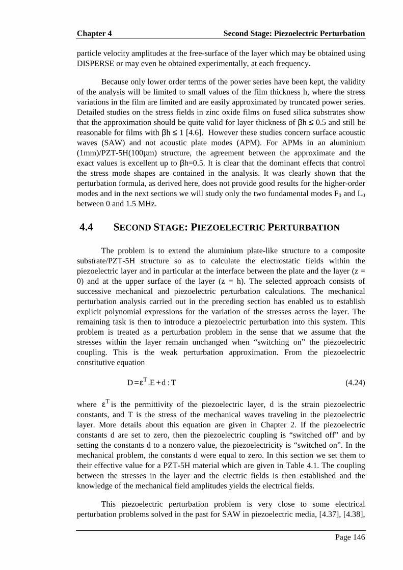
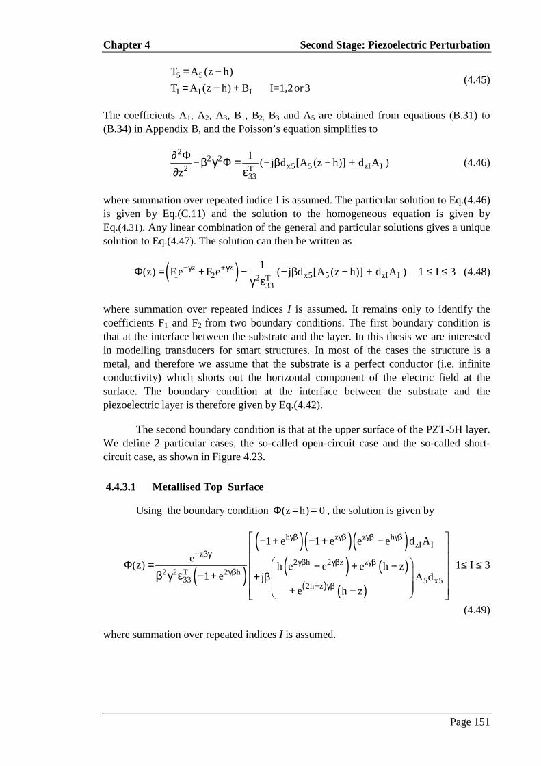
4.4 SECOND STAGE: PIEZOELECTRIC PERTURBATION.......................................................................1464.4.1 Stress Fields as Driving Terms for the Poisson Equation ................................................1474.4.2 Boundary Conditions ........................................................................................................1494.4.3 Solution of the Poisson Equation......................................................................................1504.4.4 Finite Element Validation.................................................................................................155
4.5 DISCUSSION ABOUT THE VARIOUS ASSUMPTIONS AND APPROXIMATIONS USED ........................1584.6 TRANSDUCER PROBLEM..............................................................................................................160
4.6.1 Normal Mode Expansion ..................................................................................................1624.6.2 Transmitter Problem .........................................................................................................1664.6.3 Transducer Analysis. ........................................................................................................1684.6.4 Surface Charge Distribution on a Single Strip..................................................................1744.6.5 Finite Element Validation.................................................................................................1804.6.6 Alternative Calculations ...................................................................................................1814.6.7 Conclusion ........................................................................................................................182
4.7 SCATTERING ...............................................................................................................................1824.7.1 Theoretical Basis ..............................................................................................................1844.7.2 Problem Statement and Solution.......................................................................................187
Page III
4.7.3 Finite Element Validation.................................................................................................1914.8 CONCLUSION...............................................................................................................................192REFERENCES.........................................................................................................................................194TABLES.................................................................................................................................................201FIGURES ...............................................................................................................................................202
CHAPTER 5 INTERDIGITAL TRANSDUCER FOR ACOUSTIC PLATE MODES ..................247
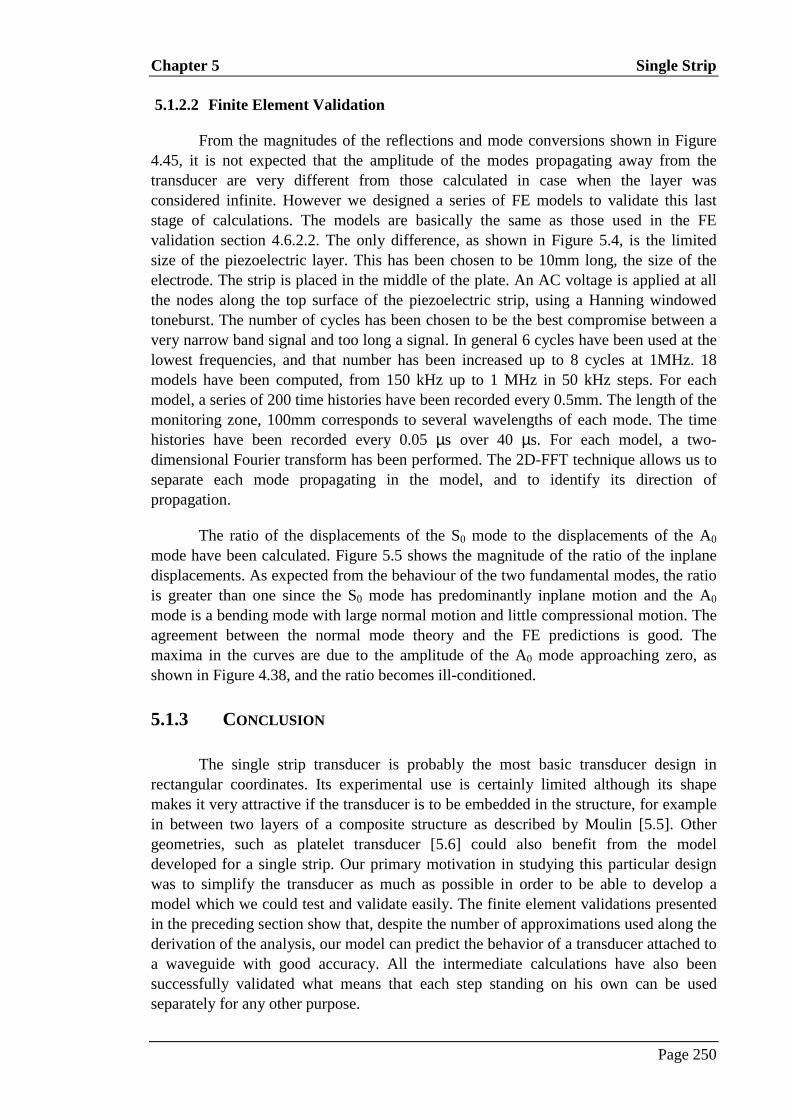
5.1 SINGLE STRIP ..............................................................................................................................2475.1.1 Problem Statement............................................................................................................2485.1.2 Full Transducer Model......................................................................................................2495.1.3 Conclusion ........................................................................................................................250
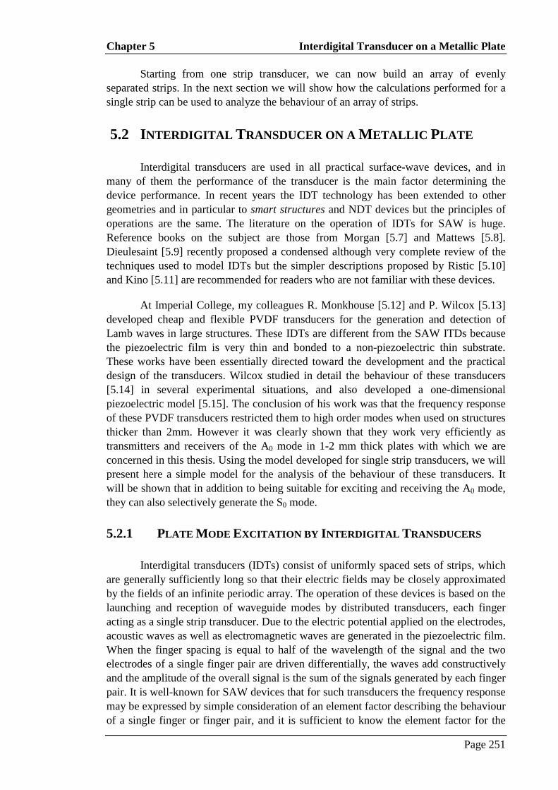
5.2 INTERDIGITAL TRANSDUCER ON A METALLIC PLATE..................................................................2515.2.1 Plate Mode Excitation by Interdigital Transducers...........................................................2515.2.2 Radiation Conductance of the Transducer ........................................................................256
5.3 EXPERIMENTAL VALIDATION AND FINITE ELEMENT INVESTIGATION .........................................2575.3.1 PVDF Material Constants.................................................................................................2585.3.2 Experimental and Finite Element Setup............................................................................2595.3.3 Processing of the Finite Element Results..........................................................................260
6.1 REVIEW OF THE THESIS ...............................................................................................................2886.2 EVALUATION...............................................................................................................................289
6.2.1 Finite element model ........................................................................................................2906.2.2 Analytical Model ..............................................................................................................2906.2.3 Wave Amplitude and Transducer Performance ................................................................291
6.3 SUMMARY OF MAIN CONTRIBUTIONS .........................................................................................2916.4 FUTURE WORK............................................................................................................................292
6.4.1 Finite Element Model .......................................................................................................2926.4.2 Transducer Model.............................................................................................................2926.4.3 New Transducer Designs .................................................................................................2936.4.4 Scattering Calculations .....................................................................................................2936.4.5 Coupling of the Analytical Model and the Finite Element Program.................................293
APPENDIX A FE77 INPUT FILE......................................................................................................295
APPENDIX B DETERMINATION OF THE STRESS FIELDS.....................................................297
APPENDIX C SOLUTION OF THE POISSON EQUATION.........................................................302
APPENDIX D ELECTRICAL BOUNDARY PERTURBATION ...................................................305
APPENDIX E INTERIOR PERTURBATION APPROACH TO THE S-PARAMETERS..........309
APPENDIX F ELECTRIC FIELD SPATIAL DISTRIBUTION.....................................................311
Page IV
List of Figures
Figure 1.1 : Interdigital transmitter and receiver on a metallic plate. .................................................25
Figure 1.2 : Schematic diagram of an interdigital electrode transducer on a metallic plate...............26
Figure 1.3 : Schematic diagram of a single strip transducer on a metallic plate. ................................27
Figure 2.1 : Diagram of flat isotropic plate, showing orientation of axes, with propagationdirection and wavefront. .................................................................................................49
Figure 2.2 : Examples of the four basic types of piezoelectricity coupling terms (from B. Auld[2.7]). ..............................................................................................................................50
Figure 3.1 : Linear acceleration...........................................................................................................99
Figure 3.3 : FE77 program architecture ............................................................................................100
Figure 3.4 : Schematic representation of a long slender rod submitted to an axial electric field,E3. Elastic conditions for the calculation of fundamental mode coupling factor are:
1 2T T 0= = , 3T 0≠ and 1 2 3S S S 0= ≠ ≠ . ..............................................................101
Figure 3.5 : Schematic representation of a thin plate submitted to a through thickness electricfield, E3. Elastic conditions for the calculation of thickness mode coupling factorare: 1 2S S 0= = ; 3S 0≠ and 1 2 3T T 0; T 0= ≠ ≠ . ..................................................101
Figure 3.6 : Schematic representation of the geometry and the coordinate system used. .................102
Figure 3.7 : Time history and corresponding amplitude spectrum of the 5-cycle toneburstapplied at all nodes on plane x = 0................................................................................103
Figure 3.8 : Predicted time history at x = 25 mm, when the input was designed to excite only thelongitudinal wave, (a) displacement in the x direction with no piezoelectricity, (b)displacement in the x direction with piezoelectricity and (c) corresponding electricpotential. .......................................................................................................................104
Figure 3.9 : Envelopes of the first wave packets taken from (a) Figure 3.8(a) and (b) Figure3.8(b).............................................................................................................................105
Page V
Figure 3.10 : Predicted time history at x = 25 mm, when the input was designed to excite only ashear wave, (a) displacement along x with no piezoelectricity, (b) displacementalong x with piezoelectricity, and (c) corresponding electric potential. .......................106
Figure 3.11 : Comparison between the group velocity dispersion curves for aluminium and foraluminium with the C11 stiffness constant piezoelectrically stiffened (ex1 = 40.46). ....107
Figure 3.12 : Predicted time history when the input was designed to excite only the S0 mode, (a)displacement in the aluminium plate, (b) displacement in aluminium with the C11
stiffness constant piezoelectrically stiffened (ex1 = 40.46), (c) displacement in analuminium plate with the stiffness constant C11 doubled, (d) electric potentialcorresponding to (b)......................................................................................................108
Figure 3.13 : Comparison between the group velocity dispersion curves for aluminium and foraluminium with the C66 stiffness constant piezoelectrically stiffened (ex6 = 20). .........109
Figure 3.14 : Predicted time history when the input was designed to excite only the A0 mode, (a)displacement in the aluminium plate, (b) displacement in aluminium with the C66
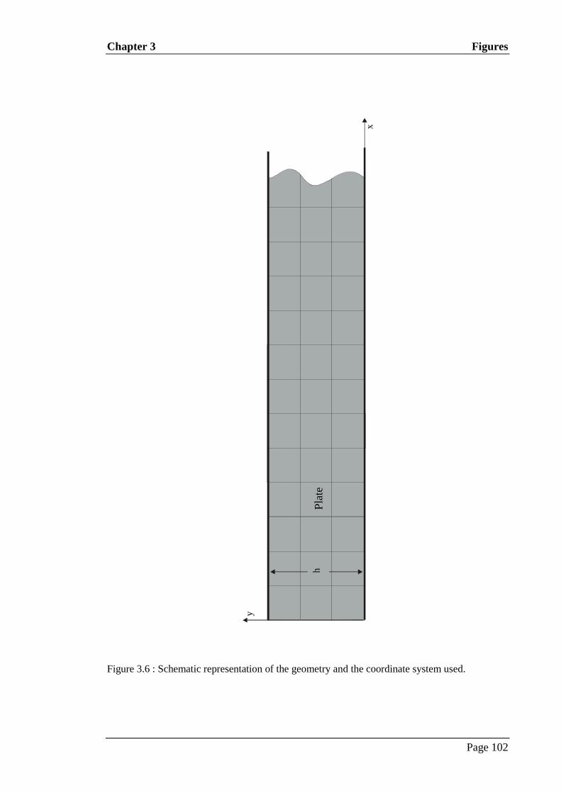
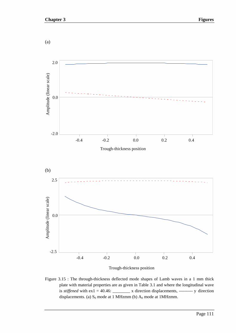
Figure 3.15 : The through-thickness deflected mode shapes of Lamb waves in a 1 mm thickplate with material properties are as given in Table 3.1 and where the longitudinalwave is stiffened with ex1 = 40.46: ________ x direction displacements, ---------- ydirection displacements. (a) S0 mode at 1 MHzmm (b) A0 mode at 1MHzmm............111
Figure 3.16 : Predicted time history, for x-direction displacements, at x = 18mm in a 1mm platewhen the input is designed to excite both the A0 and the S0 modes at 1 MHz. ............112
Figure 3.17 : Surface plot of the 2-D FFT results of the case given in Figure 3.16. Reflectedwaves are plotted with negative wavenumbers. Wavenumber dispersion curves areoverlaid. ........................................................................................................................113
Figure 3.18 : Schematic diagram of the clamped piezoelectric strip model......................................114
Figure 3.19 : Displacement profile at the free face. (a) Comparison between theoretical resultsand displacements, in the z direction, predicted using FE77 and PZFlex® (b)Comparison between FE77 and PZFlex® in the x direction. .......................................115
Figure 3.20 : The induced transient voltage response across the LiNbO3 free strip to the chargepulse of 0.0525 µs.........................................................................................................116
Figure 3.21 : Frequency spectrum of the charge impulse (1 cycle at 20 MHz) and frequencyspectrum of the predicted voltage response at the surface top electrode of theLiNbO3 free strip..........................................................................................................117
Figure 3.22 : Comparison of the predicted electrical input impedance of the LiNbO3 free stripby FE77( _____ ) and PZFlex® ( ------- ). Only the first mode of vibration isshown............................................................................................................................118
Page VI
Figure 3.23 : Schematic diagram of the model, of a piezoelectric strip mounted on a plate, usedin FE77. ........................................................................................................................119
Figure 3.24 : (a) Time trace of the input signal, a 5 cycle toneburst in square window at 900kHz, (b) frequency bandwith of the input toneburst. ....................................................120
Figure 3.25 : Group velocity dispersion curves of the Lamb modes in a 1mm thick aluminiumplate with, overlaid, the frequency spectrum of the excitation signal...........................121
Figure 3.26 : Time history of the displacement in the z direction predicted by (a) FE77 at x =50mm, (b) PZFlex at x = 50 mm, (c) FE77 at x = 99.8 mm and (d) PZFlex at x =99.8 mm. .......................................................................................................................122
Figure 3.27 : Maximum displacement profiles. Comparison between the displacementspredicted by FE77 and PZFlex (a) in the z direction, (b) in the x direction.Horizontal lines show the average value over the distance. .........................................123
Figure 3.28 : Surface plot of the 2D-FFT results of the displacements in the y direction at the topsurface of the plate. Wavenumber dispersion curves overlaid. ....................................124
Figure 4.1 : Modelling of the transducer (a) by an infinite three-layered plate (b). (c) Shows thepurely mechanical system, while the purely electrical system is shown in (d). ...........202
Figure 4.2 : Schematic diagram showing the progression of the analysis.........................................203
Figure 4.3 : Perturbation of the upper mechanical surface (y = 0) by a thin film isotropicoverlay, (a) the infinite perturbed structure, (b) coordinate system and modespropagating in the unperturbed plate, (c) coordinate system and modes propagatingin the perturbed system.................................................................................................204
Figure 4.4 : Comparison between the exact attenuation dispersion curves and the approximatewavenumber dispersion curves for the 1.2mm thick aluminium plate loaded withwater on one face. .........................................................................................................205
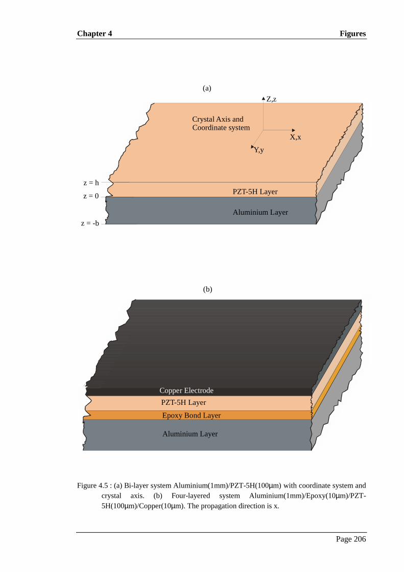
Figure 4.5 : (a) Bi-layer system Aluminium(1mm)/PZT-5H(100µm) with coordinate system andcrystal axis. (b) Four-layered system Aluminium(1mm)/Epoxy(10µm)/PZT-5H(100µm)/Copper(10µm). The propagation direction is x. .......................................206
Figure 4.6 : Comparison between the exact dispersion curves for an aluminium plate (1mmthick) and the exact dispersion curves for the aluminium(1mm)/PZT(0.1mm)system. ..........................................................................................................................207
Figure 4.7 : Spatial distribution of the power flow, for the two fundamental modes, in the bi-layered structure aluminium(1mm)/PZT(100µm). .......................................................208
Figure 4.8 : Comparison between the exact dispersion curves and the approximate dispersioncurves for the aluminium(1mm)/PZT(0.1mm) system. ................................................209
Page VII
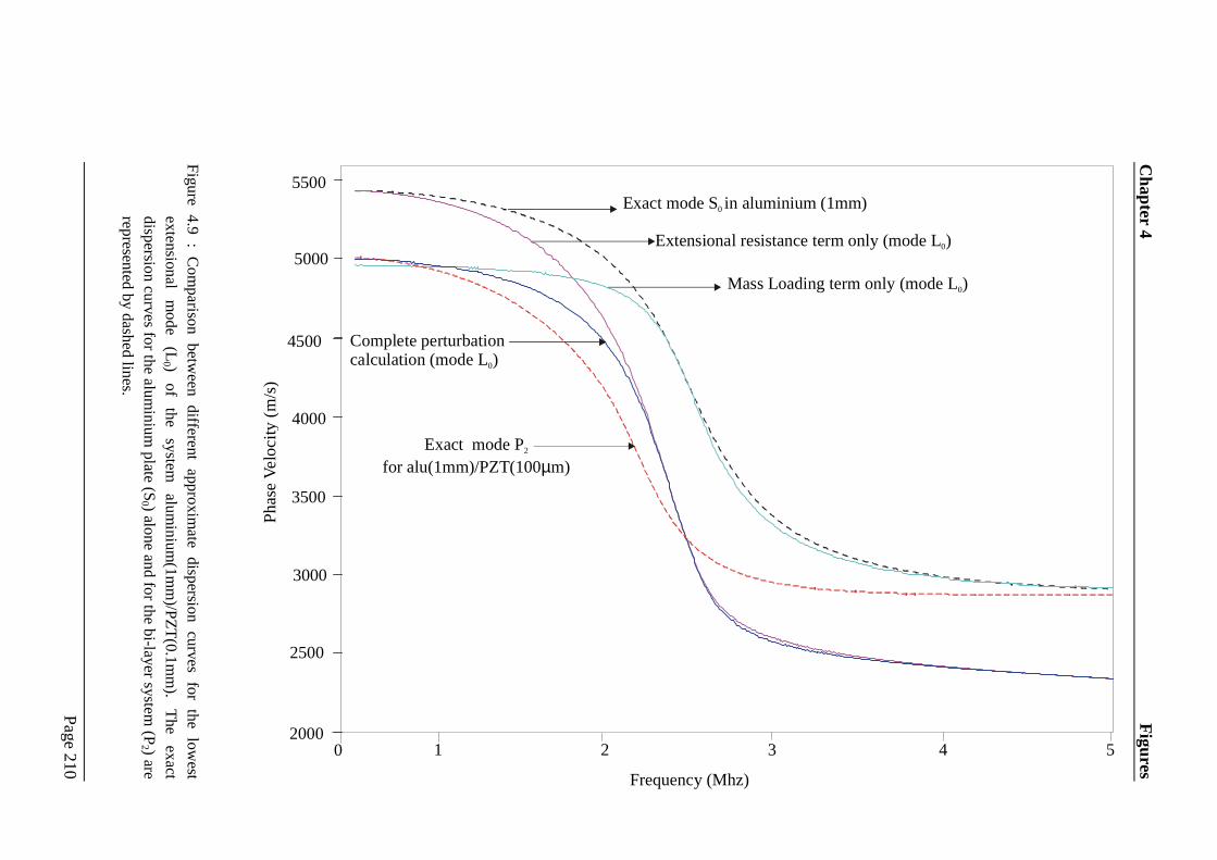
Figure 4.9 : Comparison between different approximate dispersion curves for the lowestextensional mode (L0) of the system aluminium(1mm)/PZT(0.1mm). The exactdispersion curves for the aluminium plate (S0) alone and for the bi-layer system(P2) are represented by dashed lines. ............................................................................210
Figure 4.10 : Comparison between the exact dispersion curves and the approximate dispersioncurves for the steel(1mm)/epoxy(0.1mm) system. .......................................................211
Figure 4.11 : Stress mode shapes in 100µm the PZT-5H layer. (a),(c) and (e) show the modeshapes for the mode P1, (b), (d), (f) show the mode shapes for the mode P2. (a)and (b) inplane stress mode shapes, (c) and (d) normal stress mode shapes and (e)and (f) shear stress mode shapes. Plain lines represent the stress at 0.5 MHz anddashed lines represents the stress at 2MHz...................................................................212
Figure 4.12 : Normal particle velocity dispersion curves for the aluminium(1mm)/PZT(100µm)system. Comparison between dispersion curves at the top surface of the PZT layerand the dispersion curves at the interface between the aluminium and the PZTlayer. The dispersion curves for the single 1mm aluminium plate are also shown.All curves have been calculated for a mode with unit power flow...............................213
Figure 4.13 : Inplane particle velocity dispersion curves for the aluminium(1mm)/PZT(100µm)system. Comparison between dispersion curves at the top surface of the PZT layerand the dispersion curves at the interface between the aluminium and the PZTlayer. The dispersion curves for the single 1mm aluminium plate are also shown.All curves have been calculated for a mode with unit power flow...............................214
Figure 4.14 : Stress dispersion curves for the modes F0 and P1. Comparison between the exactstress dispersion curves and the approximate stress dispersion curves for thealuminium(1mm)/PZT(100µm) system. The approximate dispersions curves havebeen obtained using the exact velocity fields. (a) Inplane stress at the top surface ofthe PZT layer, (b) inplane stress at the interface between the aluminium plate andthe PZT layer. (c) normal stress at the interface and (d) shear stress at the interface.All curves have been calculated for a mode with unit power flow...............................215
Figure 4.15 : Stress dispersion curves for the modes L0 and P2. Comparison between the exactstress dispersion curves and the approximate stress dispersion curves for thealuminium (1mm)/PZT(100µm) system. The approximate dispersions curves havebeen obtained using the exact velocity fields. (a) Inplane stress at the top surface ofthe PZT layer, (b) inplane stress at the interface between the aluminium plate andthe PZT layer. (c) normal stress at the interface and (d) shear stress at the interface.All curves have been calculated for a mode with unit power flow...............................216
Figure 4.16 : Comparison between the exact dispersion curves and the approximate dispersioncurves using the exact velocity fields for the steel(1mm)/epoxy(100µm) system........217
Figure 4.17 : Comparison between the exact wavenumber dispersion curves and theapproximate wavenumber dispersion curves for the aluminium(1mm)/PZT(50µm)
Page VIII
system. The approximate dispersions curves have been obtained using the zeroorder particle velocity amplitudes.................................................................................218
Figure 4.18 : Comparison between the exact wavenumber dispersion curves and theapproximate wavenumber dispersion curves for the aluminium(1mm)/PZT(50µm)system. The approximate dispersions curves have been obtained using the exactfree-surface particle velocity amplitudes. .....................................................................219
Figure 4.19 : Comparison between the exact wavenumber dispersion curves and theapproximate wavenumber dispersion curves for the aluminium(1mm)/PZT(100µm)system. The approximate dispersions curves have been obtained using the zeroorder particle velocity amplitudes.................................................................................220
Figure 4.20 : Comparison between the exact wavenumber dispersion curves and theapproximate wavenumber dispersion curves for the aluminium(1mm)/PZT(100µm)system. The approximate dispersion curves have been obtained using the exactfree-surface particle velocity amplitudes. .....................................................................221
Figure 4.21 : Comparison between the exact wavenumber dispersion curves and theapproximate wavenumber dispersion curves for the aluminium(1mm)/Epoxy(10µm)/PZT(100µm)/ Copper(10µm) system. The approximate dispersion curveshave been obtained using the exact free-surface particle velocity amplitudes. ............222
Figure 4.22 : (a) Exact group velocity dispersion curves for the Aluminium/Epoxy system. (b)Exact group velocity dispersion curves for the Aluminium/Epoxy/PZT-5H system. ..223
Figure 4.23 : Electrical boundary conditions in (a) the free-surface case, (b) the metallised caseat the upper surface. In both cases the metal plate is grounded and the potential iszero at the interface.......................................................................................................224
Figure 4.24 : Electric potential at the top surface of the PZT-5H layer. ...........................................225
Figure 4.25 : Schematic diagram of the finite element model used to monitor the electricpotential at the top surface of the PZT-5H layer...........................................................226
Figure 4.26 : Comparison between finite element predictions and perturbation theorycalculations for the electric potential at the top surface of the PZT-5H layer,normalised to a wave amplitude of 1 nm in the direction of propagation. Dashedline curves were obtained using the particle velocities at the top of the aluminiumplate alone and plain line curves were obtained using the particle velocities at thetop of the PZT-5H layer................................................................................................227
Figure 4.27 : (a) Exact phase velocity dispersion curves for the Aluminium/PZT-5H system. (b)Exact group velocity dispersion curves for the Aluminium/PZT-5H systemshowing the cut-off frequencies....................................................................................228
Figure 4.28 : Time domain traces of the inplane displacement of the mode P2, at 1.5 MHz, afterit has propagated over 67.5 mm. (a) Finite element prediction. (b) Simulation with
Page IX
the mode P2 propagating alone. (b) Simulation with the modes P2 and P3
Figure 4.29 : Schematic diagram (a) of the transducer problem when a potential is applied at thetop electrode. (b) Electrical boundary conditions and coordinate system. ...................230
Figure 4.30 : Excitation of plate modes by (a) distributed surface tractions, (b) by electricalcharges. .........................................................................................................................231
Figure 4.31 : Simplified representation of a bulk wave transducer without electrical andmechanical losses. The inductance is added to cancel the capacitance. .......................232
Figure 4.32 : Uniform interdigital electrode arrays and circuit interactions. The finger width is Land the spacing between two finger pair is L. ..............................................................233
Figure 4.33 : Equivalent circuit for interdigital transducer. ..............................................................234
Figure 4.34 : V V∆ for a PZT-5H thin layer (h= 0.1mm) on a grounded plane, as a function ofthe thickness to wavelength ratio, for the plate modes P1 and P2. V V∆ calculatedusing the formula for APM in plain lines, V V∆ calculated with the formula forSAW in dashed lines.....................................................................................................235
Figure 4.35 : (a) Microstrip structure, (b) Cross-field approximation of the electric field, (c)Electric field pattern showing the flux lines from the edge of the strip........................236
Figure 4.36 : Geometry of a single stripline between two different dielectric media surroundedwith (a) a shielded box and (b) two infinite parallel ground planes. (c) Geometry ofsingle stripline suspended over a ground plane. ...........................................................237
Figure 4.37 : Schematic diagram of the finite element model used to monitor the mechanicaldisplacements in the x- and z-directions at the top surface of the PZT-5H layerwhen a Voltage is applied at all nodes along a 10mm long electrode. .........................238
Figure 4.38 : Comparison between finite element predictions and normal mode amplitudecalculations for the displacements at the top surface of the PZT-5H layer, in thenormal (z) direction for the mode P1 (lowest flexural mode). ......................................239
Figure 4.39 : Comparison between finite element predictions and normal mode amplitudecalculations for the displacements at the top surface of the PZT-5H layer, in theinplane (x) direction for the mode P2 (lowest longitudinal mode)................................240
Figure 4.40 : Schematic representation of a single strip transducer. (b) shows the cross section inthe plane (xz) and the waves generated by the transducer............................................241
Figure 4.41 : (a) Schematic representation of incident and scattered wave; (b) Schematicrepresentation of one-dimensional transmission-reflection problem............................242
Figure 4.42 : Definition of S-parameters, (a) solution “1”, without the flaw, (b) solution “2”,with the flaw. (From Auld [4.7]) ..................................................................................243
Page X
Figure 4.43 : Incident plate modes on a thin strip overlay. (b) Generation of scattered waves bythe stress generated at the strip-substrate interface.......................................................244
Figure 4.44 : Schematic diagram of the finite element model used to monitor the mechanicaldisplacements in the x- and z-directions at the top surface of the PZT-5H layer forthe modes reflected at a 10mm long electrode..............................................................245
Figure 4.45 : Comparison between finite element predictions (empty square markers) and S-parameter calculations (plain curves) for the reflection coefficients of the mode S0
into (a) the mode S0, and into (b) A0. Reflection coefficients for the mode A0reflected into (c) S0 and into (d) A0. .............................................................................246
Figure 5.1 : Exact attenuation dispersion curves for a 1.2mm thick aluminium plate loaded withwater on one face. .........................................................................................................269
Figure 5.2 : Schematic representation of a single strip transducer. (b) Cross section in the plane(xz) and the waves generated by the transducer. ..........................................................270
Figure 5.3 : (a) Reflection and transmission of Lamb modes at a single strip. (b) Scattering at asingle strip transducer in transmitting mode.................................................................271
Figure 5.4 : Schematic diagram of the finite element model used to monitor the mechanicaldisplacements in the x- and z-directions at the top surface of the PZT-5H layer forthe modes reflected at a 10mm long electrode..............................................................272
Figure 5.5 : Comparison between finite element predictions and normal mode amplitudecalculations for the ratio of displacements of the S0 mode to the displacement of theA0 mode. The ratio S0/A0 is taken at the top surface of the aluminium plate anddisplacements are monitored in the inplane x-direction. ..............................................273
Figure 5.6 : Schematic diagram of an interdigital electrode transducer on a thin metallic plate. .....274
Figure 5.7 : Ratio of the quarter-wavelength to the piezoelectric layer thickness (100 mm) forthe two fundamental modes. .........................................................................................275
Figure 5.8 : Interdigital transducer. (a) Arrangement of the electrode array at the upper surfaceof the piezoelectric layer. (b) Boundary conditions for the elementary cell of thetransducer. (c) Shielded configuration. In all figures the metallic plate is omitted. .....276
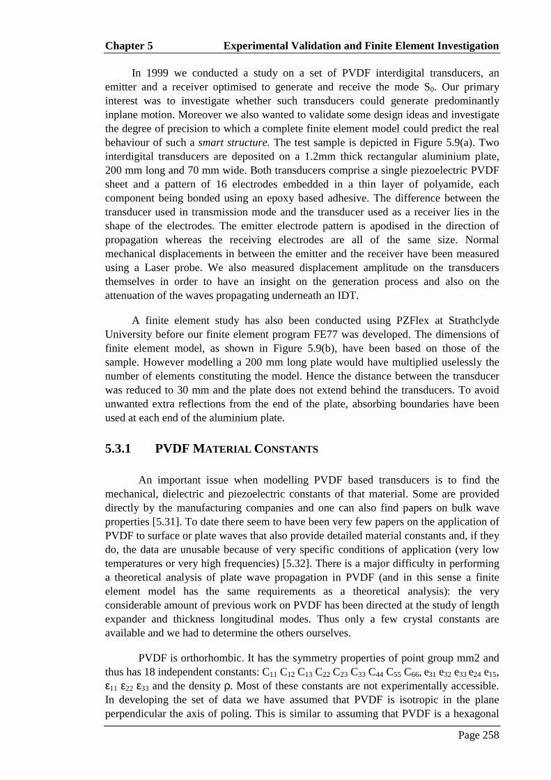
Figure 5.9 : Aluminium plate with two IDTs using PVDF piezoelectric layers and copperelectrodes. (a) Shows the experimental set up. (b) Shows the Finite element model. .277
Figure 5.10 : Dispersion curves of the first four Lamb modes for a 1.2mm thick aluminiumplate. a) Phase velocity dispersion curves, b) Group velocity dispersion curves andc) frequency versus real wavenumber curves ...............................................................278
Figure 5.11 : (a) Input voltage signal, i.e. a 8 cycle sinusoidal toneburst of centre frequency 1.3MHz. (b) Time evolution of the electrical charge distribution on the 1st electrode.The diagrams on the right show the frequency spectrum. (c) Average charge
Page XI
distribution on the grounded bottom electrode. (d) Time-frequency plot of thecharge on the bottom electrode.....................................................................................279
Figure 5.12 : Examples of snapshots of the normal displacements on the upper surface of thetransmitting IDT at different moment in time during the application of the inputsignal. The electrode pattern is shown on each snapshots. Diagrams on the right ofeach snapshot show the part of the input voltage signal applied so far. .......................280
Figure 5.13 : Experimental and predicted out-of-plane displacements on the upper surface of thetransmitting IDT. (a) Displacements measured experimentally using a laser probeon each of the electrode (black columns) and between them (gray columns). (b)Comparison between these experimental results and the displacements predictedusing the finite element model. The apodised electrode pattern is superimposed. .......281
Figure 5.14 : Measurement of the normal displacement of Lamb modes propagating in a 1.2 mmthick aluminium plate. (a) Normalised 3D plot and (b) contour view of the 2D FFTresults............................................................................................................................282
Figure 5.15 : (a), (b) and (c) out-of-plane surface displacements versus time for a 1.2mm thickaluminum plate at three different locations on the plate between the transmitter andthe receiver. ..................................................................................................................283
Figure 5.16 : Comparison of the out-of-plane surface displacements measured on the uppersurface of the aluminium plate using a Laser probe with the out-of-plane surfacedisplacements predicted using the finite element model and the absolute amplitudecalculated from the analytical model. Experimental displacements have beenmeasured every millimeter from 3 to 15mm and then at 17mm, 29mm and 30mm.....284
Figure 5.17 : Snapshots of the displacements at different times. The diagrams on the left showthe simulated displacements at the upper surface of the receiving IDT. Thediagrams on the right show the simulated displacements at the interface betweenthe plate and the IDT. ...................................................................................................285
Figure 5.18 : (a) Comparison of the simulated and measured displacements at the upper surfaceof the receiving IDT. The mean value of each series is shown. (b) Displacementsmeasured using a laser probe on the upper surface of the receiving IDT.....................286
Figure 5.19 : Displacements simulated by Finite Element at the upper surface of the receivingIDT and at the interface between the plate and the receiving IDT. Their ratio is alsoshown, superposed on the electrode pattern of the receiving transducer......................287
Page XII
List of Tables
Table 2.1 : SI Units for the main fields used in the piezoelectric constitutive equations....................48
Table 3.1: Material parameters. .......................................................................................................97
Table 3.2: Material parameters for lithium niobate - LiNbO3.........................................................97
Table 3.3: Comparison of the predicted resonance and anti-resonance frequencies of the FE77for the first mode of the LiNbO3 free strip shown in Figure 3.22..................................97
Table 3.4: Comparison of the electromechanical coupling coefficient predicted by FE77 forthe first mode shown in Figure 3.22 and the electromechanical couplingcoefficients calculated using one-dimensional approximations. ....................................98
Table 3.5: Material parameters for PZT 5H.....................................................................................98
Table 3.6: Material parameters for the aluminium plate..................................................................98
Table 4.1: Material parameters for Z-cut PZT-5H.........................................................................201
Table 4.2: Material parameters. .....................................................................................................201
Table 5.1: Material parameters for PVDF. ....................................................................................268
Chapter 1 Introduction
Page 17
Chapter 1
Introduction
The aim is to model the generation of waves by piezoelectric transducers inorder to optimise the design of electromechanical sensors used in what is fashionablycalled smart structure applications. Controversy has arisen over the use of these terms,which have been used to cover a broad range of related work in many disciplines, sincethe late 1980's. A review of work on smart structures can be found for example inCulshaw [1.1], [1.2] and recently my colleague R. Dalton [1.3] studied the possibility ofusing guided waves to monitor the structural health of an aircraft fuselage. For thisthesis, we will consider a smart structure as being a structure that has the potential tomonitor its condition repetitively. Data transport and computer technology is alreadysufficiently developed to meet the challenge of developing a smart structure for manyapplications, and they will undergo tremendous progress in the future, especially in thedata transfer area with the bluetooth new technology. However sensor technology is notyet advanced enough and recent reviews state that fully adaptive systems may not be inservice for several years [1.4]. In this thesis we will focus our attention onelectromechanical sensors and their interaction with the structure on which they areattached.
Much research has been devoted to problems in electromagnetism and acoustics.Often the investigation runs along parallel lines, the main differences being due to thevector character of the electromagnetic field and to the scalar nature of sound waves.Some times these differences are significant because of boundary conditions but oftenthe analysis is very similar, especially when the electromagnetic field is a simplefunction of time and space. For this study, we use many electromagnetic-acousticanalogies as defined by Auld [1.5]. Transducers of interest in this thesis arepiezoelectric. The piezoelectric effect is basically understood to be a result of linearinteraction between the mechanical and electrical systems, and studies on it are closelyrelated to the linear response theory. The piezoelectric direct effect manifests itself
Chapter 1 Advantages of Lamb Waves Inspection Techniques
Page 18
experimentally by the appearance of bound electric charges at the surface of the strainedmedium. The direct piezoelectric effect is always accompanied by the conversepiezoelectric effect, whereby a solid becomes strained when placed in an electric field.Piezoelectricity is a fundamental process of electromechanical interaction and isrepresentative of linear coupling in energy conversion. Obviously piezoelectricity is notthe only principle on which electromechanical devices can operate but phenomena suchas electrostriction, triboelectricity and Seigneto-electricity [1.6] are not covered in thisthesis. Hence this analysis of electronic devices necessitates knowledge in threedifferent fields of physics: mechanics, electromagnetism and piezoelectricity andassociated mathematical developments.
1.1 ADVANTAGES OF LAMB WAVES INSPECTIONTECHNIQUES
The use of ultrasonic Lamb waves for the testing of plate and pipe structures isattractive since a large area of structure can be interrogated from only a few locations.The main advantage of Lamb waves is that both sides, as well as the interior of thestructure, can be sensed from only one location on one side of the structure, whichmakes in situ monitoring viable. Many techniques such as angle transducers or EMATsare very efficient in order to excite Lamb waves in plate or pipe structures. However,for cost and dimension reasons none of these types of transducers are suited to beingpermanently attached to a structure, which is a necessary requirement in a smartstructure application. From a design point of view, permanently attached transducersare, by nature not reusable and thus their cost must be added to that of the structurewhich they are monitoring. The transducer and the structure are bonded together with anadhesive which makes consistency of the measurements easier to achieve. This meansthat such transducers are much more suitable for accurate condition monitoring thanremovable transducers for which the coupling conditions may not be consistent fromone test to another. Since the thickness and the properties of each of the component ofsuch bonded transducers is measurable, it allows us to develop a model that might beusable for any permanently attached transducer.
1.2 PERMANENTLY ATTACHED TRANSDUCERTECHNOLOGY FOR SMART STRUCTURES
Current sensor technology is well advanced in the acoustic field, but the specificapplication to the generation and reception of Lamb waves in non-piezoelectricstructures by means of piezoelectric transducers needs some further theoreticaldevelopment in order to predict accurately field parameters such as amplitude andattenuation. The generation and reception of Surface Acoustic Waves (SAW) by meansof interdigital electrodes plated on piezoelectric substrates has been widely used in theelectronics industry, [1.5], [1.7], [1.8], [1.9], [1.10]. This technology has made theconcept of using permanently attached transducers for the generation and reception ofLamb waves in a structure for NDT purposes viable. There is a special emphasis onsurface acoustic wave applications. Those waves are confined in close proximity to onesurface of the substrate and are therefore efficiently excited by acoustic and electricsources on the surface. Surface acoustic wave transducer technology is not directly
Chapter 1 Modelling of Field Generated by Piezoelectric Transducers
Page 19
applicable to smart structures because of the frequency at which these devices operate,normally in the GHz range, whereas NDT applications typically work below afrequency thickness product of 1 MHz-mm. Hence in order to inspect large structures,flexible cheap PVDF transducers have been developed for the generation and thedetection of Lamb waves, [1.11], [1.12]. The geometry of these devices is similar to thatof the transducers used to generate surface acoustic waves in non-piezoelectricsubstrates, see [1.13] and [1.14]. The plate under interrogation is overlaid by a thinpiezoelectric film, itself overlaid by the interdigital electrodes. The transducercomprises the piezoelectric film and the electrodes, where the piezoelectric film is verythin and is limited in the two other dimensions to the size of the electrodes. Figure 1.1shows this configuration for Lamb modes.
1.3 MODELLING OF FIELD GENERATED BYPIEZOELECTRIC TRANSDUCERS
From the above discussion, the main goal of this thesis appears as being toinvestigate the process by which permanently attached transducers can generate guidedwaves in structures. Our interest in this particular subject, and the particular directionwe took to study it, follow from the chief objective and the main conclusions we drewfrom a project [1.23] founded on an EPSRC/DIG Grant which was entitled "EfficientUltrasonic Inspection and Monitoring of Large Structures”. This project linked togetherthe combined efforts of several researchers from Strathclyde University [1.15] andImperial College, efforts that were orientated toward a common goal: producingpermanently attached sensors to monitor large structures which involved optimisation ofthe form of the sensors, the determination of the best mode(s) to use and thedevelopment of test strategies (e.g. pulse-echo).
The work at Imperial College concentrated on the modelling of the behaviour ofthe transducers, the development of inspection strategies and the refinement of PVDFbased permanently attached sensors. Figure 1.2 shows a schematic diagram of suchtransducers, with interdigital electrodes, on a metallic plate. The aim was to producepermanently attached sensors, which could generate modes whose motion ispredominantly in-plane. However it was found that this was considerably more difficultthan had been anticipated. Facing these difficulties led during the growth of the projectto re-direction of the work away from developing interdigital PVDF based sensors. Theoperation of these devices is based on the launching and the reception of wave guidemodes by distributed electrodes. One of the reasons why such transducers are difficultto model is that the function that describe the charge distribution is extremelycumbersome [1.19], [1.20], [1.21], [1.22] and the number of parameters that affect theresponse of such a transducer is large. Solutions exist, such as those provided by Engan[1.21] and Coquin [1.22] for example, but they are valid only for SAW and not forLamb waves and these solution still needed to be developed. Therefore we believed thatwe could gain in understanding and time by starting the study to a less cumbersomeproblem. Indeed, at first approximation each of the distributed sources (i.e. eachelectrode) of the IDT transducer is acting as a single transducer. Such an elementarytransducer, referenced as a strip transducer by analogy with transmission line strips, is
Chapter 1 Modelling of Field Generated by Piezoelectric Transducers
Page 20
easier to study, at least from the mathematical point of view. Figure 1.3 shows theconfiguration for a single element. Nonetheless if the electrostatic problem is greatlysimplified for such a transducer, the mechanical problem is the same as for an IDT. Thesystem is multilayered, limited in extend, and the guided waves generated in thestructure are dependent on the mechanical and electrical waves generated inside andunderneath the transducer. However we are not so much interested in what happensexactly in the transducer itself. Thus is possible to use some simplifying approximationsin order to obtain information only about the fields that we are primarily interested in.This, in theory, should allow us to get the physical understanding of what is happeningin the overall system.
It has also been shown during the EPSRC founded project [1.23] thatsatisfactory field predictions could be obtained by assuming that the analysis of thePVDF based interdigital transducer can be decoupled from that of the structure and thatthe action of the IDTs is essentially to apply out-of-plane forces at the locations of thefingers. Accordingly non-piezoelectric finite element or Huygens’ principle basedcalculations [1.16] enable us to predict efficiently the field generated in the structureand a 1-D piezoelectric transmission line technique enable to analyse the electricbehaviour of piezoelectric sensors [1.17]. Although these assumptions are valid in largenumber of circumstances, the amplitude of the acoustic wave generated by a givenvoltage applied to the transducer and vice-versa cannot be predicted using the modelsaforementioned. Moreover these approximation are fair for low acoustic impedance andweak electromechanical coupling transducer materials such as PVDF [1.11], [1.12], butit is very unlikely to remain accurate for ceramic-based transducers. It was thereforedecided to develop more accurate models and this is achieved by two different means.The first one is to develop a finite element program allowing to model the fullpiezoelectric behaviour. The second one is to develop an analytical model that willenlighten the key factors governing the performance of the transducers.
1.3.1 FINITE ELEMENT ANALYSIS
The Strathclyde group uses a commercially available FE code, PZFlex whichcan perform dynamic piezoelectric analysis in the time domain, as required in thisstudy, but, although very efficient, PZFlex is not optimized for Lamb wave work. Thisis a problem common to most commercially available codes and it is usually impossibleto modify the source of such codes. Hence it was decided to incorporate piezoelectricityin an already existing general purpose finite element package, FE77 [1.25] developed atImperial College by Mr. D. Hitchings for thermal and structural analysis. On previousprojects [1.26], [1.27], this code has been optimized at the NDT Lab for the solution ofLamb wave propagation problems in the time domain. Unfortunately it did not allowpiezoelectric equations to be solved so this feature was added. From the generalformulation of finite element piezoelectric equations found in the literature, we deriveda direct integration formulation based on the central difference explicit methods ofintegration. Although simple in its principle, implementation of a new set of equationsin an already existing finite element code required lots of attention. FE77 is a researchtool, constantly under development for more than 20 years, and despite the constant
Chapter 1 Thesis Outline
Page 21
help of Mr. D. Hitchings a considerable amount of time was spent on understanding theoriginal code and tracking coding errors. Nevertheless the code is now producingpiezoelectric calculations and results are systematically being validated against simpleexamples. Although the introduction of the piezoelectric equations in FE77 will mainlyserve the purpose of validating the analytic model it is to be mentioned that it has beendeveloped in the form of a permanent module of FE77 in order to be used by otherresearchers in the future.
A major drawback of the finite element technique is that this does not runquickly enough to be used as an interactive design tool. Moreover the solution providedis purely numerical, hiding most of the physical significance of the electromechanicalcoupling process. Hence an analytic approach of the problem was undertaken.
1.3.2 ANALYTICAL MODEL
This model was initially only concerned with PVDF based interdigitaltransducers (IDTs). However it is believed that the analytic work carried out for IDTscan be diverted from its initial aim to enlighten our comprehension of the physicsinvolved in electromechanical coupling within ceramic based piezoelectric transducers.The reason for that is that basically a piezoelectric transducer always comprises apiezoelectric layer, adhesive layers and electrodes. The mathematical difficulty with thestudy of IDT resides entirely in the formulation of the electric charge distribution. If onecompare the strip transducer geometry shown in Figure 1.3 and the geometry of the IDTtransducer shown in Figure 1.2, it appears that the difference lies only in the electrodepattern. By comparison with an IDT, the electrical boundary problem is simplified forthe single strip transducer but the rest of the study is identical. Therefore we decided todevelop an analysis for the strip transducer bearing in mind that this study can beextended to many other transducers as long as their geometries are similar to that of thesingle strip transducer, that is basically a stack of layers of finite thickness and lateraldimensions. Due to the voltage applied across the electrodes, acoustic waves as well aselectromagnetic waves are generated in the piezoelectric layer. However, we are notprimarily interested in the exact behavior of the film so it is appropriate to make somesimplifying assumptions about the piezoelectric layer/electrode structure in order toobtain a physical understanding of what is happening in the overall system. Theseassumptions are related to the perturbation theory and they allow keeping the modelanalytical. Keeping the problem analytical enable to determine appropriate transducerproperties in order to generate a given mode with a given amplitude in a given structure.
1.4 THESIS OUTLINE
The thesis will investigate some aspects of the fundamental science necessary forthe development of piezoelectric sensors for use in integral structural inspectionsystems based on the use of ultrasonic Lamb waves. It will be particularly concernedwith the analysis of the electromechanical interaction and the process of generation ofLamb waves and the design of permanently attached transducers such as ceramic-basedpiezoelectric discs or IDT's. This work naturally fell into phases defined by the
Chapter 1 Thesis Outline
Page 22
development of the tools and theories needed to investigate the behaviour ofpiezoelectric transducers. These phases of work therefore form the subsequent chaptersof this thesis. There are six chapters, the first being this introduction chapter.
Lamb waves, which are the guided waves of a free plate, are considered inChapter 2, where attention focuses on their modal properties. Structures of interest insmart structure technologies are closely related to free plate structures and the presenceof the transducers only affect the guided wave locally. As shown by Auld [1.5] modalanalysis is a powerful tool for treating waveguide excitation and scattering problems.As stated by Auld, in order to apply this technique in electrodynamics, one mustdevelop a procedure based on the reciprocity relationship and mode orthogonality, forexpanding arbitrary acoustic waveguide field distributions as superposition ofwaveguide modes. These techniques are also presented in Chapter 2. The well-knownperturbation theory is also presented since this is the approximate method used todevelop the analytic model for waveguide excitation by means of piezoelectrictransducer. Lastly, piezoelectric materials used in this study are presented and a shortreview of the piezoelectric equations is given.
A finite element formulation that includes the piezoelectric or electroelasticeffect along side with the dynamical matrix equation of electroelasticity and itsreduction to the well-known equation of structural dynamics, based on a strong analogybetween electric and elastic variables, is developed in Chapter 3. It is shown how theseequations were incorporated in an already existing finite element code [1.25]. Thisprogram has been checked against PZFlex [1.28] and the validation results arepresented.
In Chapter 4, the analytical model, developed on the basis of normal modetheory and perturbation methods for predicting the acoustic field generated by a givenvoltage applied to a transducer and vice-versa, is presented. The sections follownaturally the three perturbation steps of the model, and insight is given on how eachperturbation step can be used for various independent problems. Since the overall modelis based on assumptions mainly related to the perturbation methods, these are discussedand limits of the model as well as its eventual extensions will be drawn. Throughout thedevelopment of the model, validation against the finite element program will bepresented.
In Chapter 5, a full example of the structure of interest in this study is presented.Comparison between the results obtained from the analytical model and the finiteelement program is presented. This example serves the purpose of fully validating theanalytical model presented in Chapter 4. Preliminary Results on the analysis and theexperimental study of IDTs are also presented.
Lastly, Chapter 6 presents the conclusions of this thesis regarding the modellingof the generation of guided waves by piezoelectric transducers. The approach and themethods used throughout this work are also critically reviewed and a number ofavenues for further work are suggested, in particular concerning the modelling ofguided waves scattering at surface defects such as notches, grooves or cracks.
[1.2] Culshaw, B., Smart Structures and Materials, Artech House, Boston and London,1996.
[1.3] Dalton, R., The Propagation of Lamb Waves Through Metallic Aircraft FuselageStructure, Ph.D. Thesis, University of London, (Imperial College, Mechanicalengineering Department), 2000.
[1.4] Chopra, I., "Review of Current Status of Smart Strucutres and Integrated Systems",SPIE, Vol. 2717, pp. 20-62, 1996.
[1.5] Auld, B. A., Acoustic Fields and Waves In Solids, Vol. II, 2nd ed., Robert E. KriegerPublishing Compagny, Malabar, Florida, 1990.
[1.6] Durand, E., Electrostatique III: Méthode de Calcul, Diélectriques, Masson & Cie,Paris, 1966.
[1.7] Kino, G. S., Acoustic Waves: Devices, Imaging and Analog Signal Processing,Prentice-Hall Inc., Englewood Cliffs, New Jersey, 1987.
[1.8] Dieulesaint, E. and Royer, D., Elastic Waves in Solids, Application to SignalProcessing; John Wiley & Son Inc., 1980.
[1.9] Morgan, D. P., Surface-Wave Devices for Signal Processing, Elsevier, Amsterdam,Oxford, New York, Tokyo, 1991.
[1.10] Matthews, H., (ed.), Surface Wave Filters, John Wiley & Sons, New York, London,Sydney, Toronto, 1977.
[1.11] Wilcox, P. D., Lamb Wave Inspection of Large Structures using Permanently AttachedTransducers, Ph.D. Thesis, University of London, (Imperial College, Mechanicalengineering Department), 1998.
[1.12] Monkhouse, R. S. C., Wilcox, P. D., and Cawley, P., “Flexible Interdigital PVDFTransducers for the Generation of Lamb Waves in Structures’, Ultrasonics, 1997.
[1.13] Kino, G. S. and Wagers, R. S., “Theory of Interdigital Couplers on Non-PiezoelectricSubstrates”, J. Appl. Phys., Vol. 44, pp. 1480-1488, 1973.
[1.14] Dieulesaint, E., Mattioco, F. and Royer, D., “Excitation et Détection d’Ondes deRayleigh á l’aide d’une Feuille de Polymère Piézoéléctrique”, C. R. Acad. Sc. Paris,Tome 287, Série B171, 1978.
[1.15] Ultrasonic Research group, Department of Electronic and Electrical Engineering,University of Strathclyde, Glasgow, U.K., G1 1XW.
Chapter 1 References
Page 24
[1.16] Wilcox, P. D., Monkhouse, R. S. C., Lowe, M. J. S. and Cawley, P., “The Use ofHuygens’ Principle to Model the Acoustic Field from Interdigital Transducers”, Reviewof Progress in Quantitative NDE, eds. D.O. Thompson and D.E. Chimenti, PlenumPress, N. Y., Vol. 17, 1998.
[1.17] Wilcox, P. D., Monkhouse, R. S. C., Cawley, P., Lowe, M. J. S. and Auld, B. A.,“Development of a Computer Model for an Ultrasonic Polymer Film TransducerSystem”, NDT & E International, Vol. 31(1), pp. 51-64, 1998.
[1.18] Gachagan, A., Reynolds, P., Hayward, G. and McNab, A., “Construction andEvaluation of a New Generation of Flexible Ultrasonic Transducers”, IEEE UltrasonicsSymposium, pp. 1-4, 1996.
[1.19] Tiersten, H. F., Linear Piezoelectric Plate Vibrations, Plenum Press, New York, 1969.
[1.20] Joshi, S. G. and Jin, Y., “Excitation of Ultrasonic Lamb Waves in Piezoelectric Plates”,J. Appl. Phys., Vol. 69, pp. 8018-8024, 1991.
[1.21] Engan, H., “Excitation of Elastic Surface Waves by Spatial Harmonics of InterdigitalTransducers”, IEEE Transaction on Electron Devices, Vol. ED16, pp. 1014-1017, 1969.
[1.22] Coquin, G. A. and Tiersten, H. F., “Analysis of the Excitation and Detection ofPiezoelectric Surface Waves in Quartz By Means of Surface Electrodes”, J. Acoustic.Soc. Am., Vol. 41, pp 921-939, 1966.
[1.23] Marty, P. N., “Analytical Analysis of Plate Modes Generated by InterdigitalCouplers on non Piezoelectric Substrates” in Efficient Ultrasonic Inspection andMonitoring of Large Structures - Progress Report on EPSRC/DIPG Grant, Appendix A,June 1997.
[1.25] Hitchings, D., “FE77 User Manual”, Internal Report, Imperial College, Department ofAeronautics, 1997.
[1.26] Alleyne, D. and Cawley, P., “The Interaction of Lamb Waves with Defects”, IEEETransactions on Ultrasonics, Ferroelectrics, and Frequency Control, Vol. 39(3), pp 491-494, 1992.
[1.27] Pavlakovic, B., Alleyne, D. N., Lowe, M. J. S., and Cawley, P., “Simulation of LambWaves Propagation Using Pure Mode Excitation”, Review of Progress in QuantitativeNDE, eds. D.O. Thompson and D.E. Chimenti, American Institute of Physics, NewYork, Vol. 17, 1997.
[1.28] Wojcik, G. L., Vaughan, D. K., Abboud, N. and Mould, J. Jr., “ElectromechanicalModelling using Explicit Time-Domain Finite Elements”, IEEE Ultrasonic SymposiumProceedings, 1993.
Chapter 1 Figures
Page 25
FIGURES
Piez
oele
ctric
laye
r
Elec
trode
s
Gui
ded
acou
stic
fiel
d
Met
allic
pla
te
Tran
smitt
erRe
ceiv
er
Figure 1.1 : Interdigital transmitter and receiver on a metallic plate.
Chapter 1
Figures
Page 26
Piezolectric layer
Applied electric potentiel
V
Electrodes
Metallic plate
Polyamide film Copper electrodes printed onto polyamide film
Epoxy bond betweenelectrodes and PVDF film
PVDF film
Epoxy bond betweenPVDF film and substrate
Figure 1.2 : Schematic diagram
of an interdigital electrode transducer on a metallic plate.
Chapter 1
Figures
Page 27
Applied electric potentiel
V
Ground electrode
Electrode Epoxy bondPiezoelectric layer
Piezolectric layer Electrode Metallic plate
Figure 1.3 : Schematic diagram
of a single strip transducer on a metallic plate.
Chapter 2 Background
Page 28
Chapter 2
Background
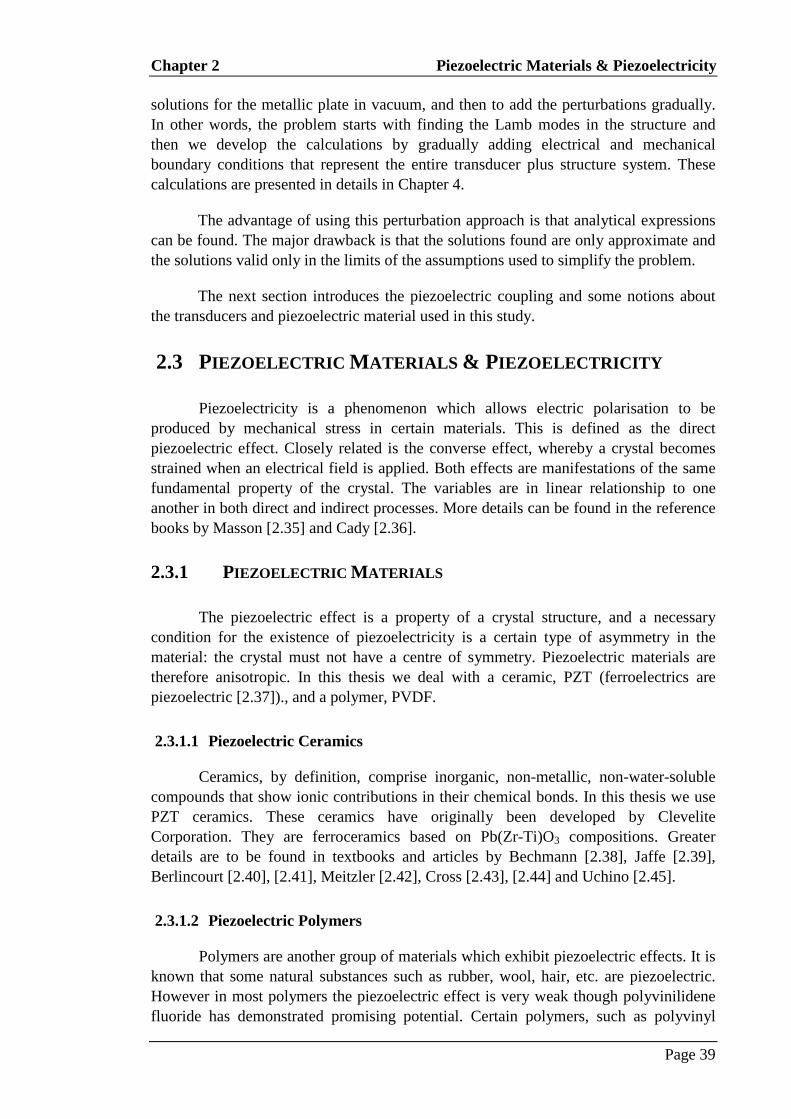
The focal point of this thesis is the analysis of the generation of Lamb waves[2.1] in plate-like structures by piezoelectric transducers, with special attention given tointerdigital transducers. We will concentrate our study on the interaction between thintransducers and the structure in which the Lamb waves propagate. In order to have acorrect idea of the fields applied by the transducer onto the structure, any interactionsbetween any mechanical and electrical fields in the transducer have to be quantified.
This chapter introduces the basic concepts and equations that, although well-known, are necessary for the understanding of the analysis developed in Chapters 3 to 5.The first section is concerned with a general description of the acoustic field in plate-like structures. The second section shows how the normal mode technique can be usedto treat waveguide excitation problems, in conjunction with the reciprocity relationship.The third section presents the perturbation techniques which are used to quantify howthe presence of a transducer influences the behaviour of the modes that propagate in thatwaveguide. The fourth and last section is concerned with transducers, the piezoelectricmaterials that constitute them and the equations of piezoelectricity.
2.1 PLATE WAVES
In this section the emphasis is on the theoretical analysis of guided wavespropagating in solids. All equations and reasoning presented here can be found in moredetails in the selection of books [2.1] to [2.15] proposed in the reference section.
In this section, and in the rest of this thesis, it is assumed that mechanical wavessuffer no attenuation due to "internal friction", i.e. material attenuation is assumed to benegligible. This condition is not too restrictive since low-loss materials are usuallychosen for practical waveguides and internal friction has a negligible effect on the
Chapter 2 Plate Waves
Page 29
velocity of propagation and other characteristics of the guided waves except for anoverall reduction in amplitude.
2.1.1 PROPAGATION IN UNBOUNDED NEDIA
The general description of guided waves starts with the definition of strain andstress, and with Hooke’s law, which describes the relation between stress and strain, andgoes on to derive the wave equation of motion. The mathematical forms of the wavesthat can propagate in a solid medium (bounded or infinite), are the solution of the waveequation. If boundaries exist, these solutions must also satisfy certain conditions at theboundaries. First we shall be concerned with unbounded media of propagation, thematerial being homogeneous, linear elastic, non-absorbing and non-piezoelectric.Contrary to rigid body dynamics that assumes that the material of the body has infiniteYoung’s modulus, i.e. that a resultant force sets every point in a body in motioninstantaneously, we shall consider the case where a body is a sum of infinitesimallysmall mass elements. These masses will vibrate in the material according to Newton’slaw applied to each of these small masses. The motion of each particle produceschanges in the equilibrium of the neighbouring particles and this cause stress, whichwill be transmitted through the medium [2.2].
2.1.1.1 Strain
Consider a point P(x1, x2, x3) in a solid body in which a wave propagateswithout any loss of amplitude. This point is displaced, the components of thedisplacement being (u1, u2, u3). Direct strains in the medium in the vicinity of P arerepresented by S11, S22 and S33 and the shear components of strain S12, S23 and S13
correspond to the rotation of the element as a rigid body. ,
The strain tensor S can be expressed in the following form, see [2.3]:
jiij
j i
uu1S i, j 1,2,32 x x� �∂∂
= + =� �� �∂ ∂� �(2.1)
The strain tensor S is symmetric and the above equation is only valid in case ofsmall deformations, a condition that will be kept valid throughout this thesis. Thevelocity at which particle P is displaced is denoted as v, and in the three directions it isfound from the particle displacement using formula:
ii
duv , i 1,2,3dt
= = (2.2)
2.1.1.2 Stress
The stress is a force over a unit area, thus the net force Fi, in the direction xi, is:
Chapter 2 Plate Waves
Page 30
iji
j
TF = i, j 1,2,3
x∂
=∂
(2.3)
where T is the stress tensor. To describe the force acting on an elemental area of a body,nine stress component are required, just as for the strain. The stress tensor, alike thestrain tensor is symmetric, i.e. ij jiT T= . The symmetry condition on both tensors impliesthat only six of the nine components are needed to fully describe the stress and strainstates of the body. Therefore instead of representing the stress and strains as a tensor ofrank 2, we use a 6 component vector. For example, the stress tensor T
xx xy xz
yx xx yz
zx zy xx
T T T
T T T
T T T
� �� �� �� �� �� �
(2.4)
is also represented by the vector
( )1 2 3 4 5 6T ,T ,T ,T ,T ,T with 1 xx 2 yy 3 zz
The general form of Hooke's law assumes that each of the six components of thestress is a linear function of six components of the strain. Therefore 36 elastic constants,cij with i,j = 1,..,6 are needed. Love [2.3] showed that the elastic tensor must besymmetric. This property reduces the number of independent elastic constants to 21. Intensor notation, Hooke's law is given by
lij ijkl kl ijkl
k
uT c S c i, j, k, l 1,2,3
x∂
= = =∂
(2.6)
and in vector notation,
I IJ JT c S I, J 1...6= = (2.7)
The most complex crystals, of the triclinic class, require these 21 elasticconstants to define the stress-strain relations, but in crystals with planes and axes ofsymmetry the number is reduced, as we will see it when discussing piezoelectriccrystals. It is indeed very fortunate that most piezoelectric materials are either cubic,hexagonal or orthorhombic, reducing the number of independent constants to 3, 6 or 9respectively. Metallic plate-like structures are often isotropic, for which the number ofindependent elastic constant is reduced to 2 Lamé's coefficients. In an isotropic solid
Chapter 2 Plate Waves
Page 31
( )12 13 21 23 31 32
144 55 66 11 122
11 22 33
c c c c c c
c c c , c c
2 c c c
λ = = = = = =
µ = = = = −
λ + µ= = =
(2.8)
and all the other coefficients are zero. Therefore, from Eq.(2.6) Hooke's law forisotropic solids is
ij ij ijT 2 S=λ∆δ + µ (2.9)
Lamé's constants λ and µ completely define the elastic stress-strain behaviour of thematerial. In engineering applications Lamé's constants are usually replaced forconvenience by four related elastic constants, [2.4] and [2.5]:
(3 2 ) 2E , , B , G ;2( ) 3
µ λ + µ λ µ= σ = =λ + =µλ + µ λ + µ
(2.10)
E E, ,(1 )(1 2 ) 2(1 )
σλ = µ =+ σ − σ + σ
(2.11)
where E is the modulus of elasticity, ν is Poisson's ratio, B is the bulk modulus and G isthe shear modulus. Lamé's constants λ and µ determine the ratio between the shearvelocity and the longitudinal velocity. This ratio, for an isotropic medium, is alwaysbetween 0 and 0.707.
2.1.1.4 The Equation of Motion
The equation of motion comes from the fundamental law of dynamics, F = mγ,where γ is the acceleration of the particle and F is a force given by Eq.(2.3). Neglectingthe effect of gravity, stating that the force applied gives raise to the acceleration of theunit volume mass ρ and making use of Hooke’s law, the equation of motion becomes:
2iji
2j
Tu =
xt
∂∂ρ
∂∂(2.12)
This equation which describes the motion in a solid is obtained by consideringstress variations across an element. It can be expressed, from equations (2.1) and (2.9),in term of the stress-strain relations as [2.6]:
2 2i l
ijkl 2j k
u u = C
t x x∂ ∂
ρ∂ ∂ ∂
(2.13)
The four-index notation for the elastic constant tensor can be contracted to the two-index notation used, for example in Eq.(2.7) in the same way the stress and straintensors have been contracted into six-component vectors. In other words, Eq.(2.13) canbe derived from Eq.(2.12) using Eq.(2.6) or (2.7). Auld [2.7] gives more details on how
Chapter 2 Plate Waves
Page 32
the divergence of stress operation and the strain-displacement relation can berepresented by a matrix in rectangular coordinates.
2.1.1.5 The Wave Equation
Further analysis of the wave equation is usually made simpler if two potentialfunctions are introduced, a scalar and a vector potential of the displacement vector.However here we will not make use of this convenient technique. As we will see it later,to be piezoelectric a crystal must be anisotropic and it is more convenient for us to useChristoffel’s equation.
In dynamic elasticity or acoustics we are interested in propagation phenomena.The equation of motion as given in Eq.(2.13) for a three-dimensional anisotropicmedium, can be seen as a generalisation of the propagation equation in a fluid [2.8]which has a general solution u(x, t)� in the form of a progressive wave, travelling in adirection n� perpendicular to the wave planes n.x = constant,� � where x� is the positionvector of the points of the wave planes. This solution,
n.xu(x,t)=A pf t-V
� �� �� �
� �
�� (2.14)
represents the vibration created at each position x� by a wave propagating in thedirection n� . V is the phase velocity, A is the amplitude of the vibration and p� the wavepolarisation (i.e. the particle displacement direction). Among all possible disturbances,harmonic vibrations about a mean position are very important since other perturbationsresult from the superposition of these vibrations [2.9]. The solution to Eq.(2.13), for afluid is sought using the separation of variables techniques. The general solution is astationary or standing harmonic wave. This solution may be put in the form of the sumof harmonic waves propagating in opposite directions. The typical form of the functionf of Eq.(2.14), assuming an initial time behavior of the form exp( t)ω is then given byexp( t -kx)ω where ω is the frequency of the vibration and k is referred to as thewavenumber. The argument ( t -kx)ω is designated as the phase and for increasing time,increasing values of x are required to maintain the phase constant. Therefore thisfunction represent a wave propagating in the positive x direction. The propagationvelocity of the planes of constant phase is the phase velocity:
kV =ω
(2.15)
The wavenumber is the inverse of the wavelength which is the space intervalwhich lies, at a given time, between two identical states of the continuum, for instancetwo successive maxima of the vibration. Therefore the quantity (kx) measures thedifference in phase at a given time between the vibration of planes separated in space bythe distance x. Graff [2.9] pointed out that a solution of type Acos( t-kx)ω has no wavefront since it represents a vibration of infinite length. Therefore it is only by consideringthe phase that a propagation velocity can be associated with the motion. Therefore,
Chapter 2 Plate Waves
Page 33
assuming solutions in the form of harmonic propagating waves, the equation of motionin its general form can be reduced to the Christoffel equation [2.7]
2 2il l ik u uΓ =ρω (2.16)
where the second rank tensor
il ijkl j kc n nΓ = (2.17)
is called the Christoffel tensor. Its elements are functions only of the plane wavepropagation direction and the stiffness constants of the medium. It applies to bulk waves(uniform plane waves). Generally, for a given direction of propagation of those bulkwaves, there are three velocities, the three roots of the secular equation
2il ilV 0Γ −ρ δ = (2.18)
which express the compatibility of the three homogeneous equations [2.10]. Eachvelocity is related to an eigenvector, which defines the direction of displacement (i.e.the polarisation of the wave).
Although we are interested in the behaviour of anisotropic crystals, it isconvenient first to consider a simple isotropic example. This exercise will be veryuseful when, in Chapter 3, we will investigate simple one-dimensional propagationalong directions linked to the piezoelectric crystal axes of symmetry. The Christoffeltensor for an isotropic infinite solid, when the stiffness matrix given by Eq.(2.8) issubstituted in Eq.(2.18), is
2 211 x 44 x 12 44 x y 12 44 x z
2 2il 12 44 x y 11 y 44 y 12 44 z y
2 212 44 x z 12 44 z y 11 z 44 z
c n c (1 n ) (c c )n n (c c )n n
(c c )n n c n c (1 n ) (c c )n n
(c c )n n (c c )n n c n c (1 n )
� �+ − + +� �� �Γ = + + − +� �� �+ + + −� �
(2.19)
Now if we assume that the wave is propagating in a particular direction, for example thedirection z, then Eq.(2.19) becomes a diagonal matrix and the Christoffel equationreduces to
There are three independent solutions, i.e. three independent waves propagatingin the z direction but polarised in different directions: an x-polarised wave and a y-polarised wave which both satisfy the dispersion relation
2 244k c =ρω (2.21)
Chapter 2 Plate Waves
Page 34
These waves are shear or transverse waves, propagating with velocity
T 44c c= ρ . The shear displacements are given by j( t kz)su p ue where p.z 0ω −= =� � � . The
third solution is a compressional wave j( t kz)lu z ue ω −=� propagating with velocity
L 11c c= ρ . The velocity cL is associated with displacement components parallel tothe direction of propagation, while cT is associated with displacement componentsnormal to the direction of propagation. The corresponding shear and longitudinal wavespropagate independently of each other. Therefore, any plane wave propagating throughan infinite isotropic medium must travel with a constant velocity (cL or cT), which is afunction of material properties only. These three solutions are independent of thedirection of propagation by virtue of the nature of isotropic solids. This is not true forgenerally anisotropic solids.
2.1.2 THE LAW OF REFRACTION OF PLANE WAVES AT AN INTERFACE
Expression of the reflection of longitudinal and shear waves incident on theboundaries is essential to the comprehension of the behaviour of guided waves. Detailson this subject may, for example, be founds in Redwood [2.11] and expressions for thereflection and transmission coefficients are given in [2.9] and [2.12].
If a plane wave strikes a plane interface obliquely, reflected and transmittedwaves arise, as in optics. If a longitudinal wave is incident at the boundary two waves, alongitudinal wave and a shear wave are generally reflected, the shear wave beinggenerated by mode conversion. If only a shear wave is incident, in general there will bemode conversion to a longitudinal wave to satisfy boundary conditions. No modeconversion occurs at normal incidence, or when the shear wave is incident at 45°. Thelaw of refraction determines the directions of the reflected and transmitted waves. Forexample if we assume that a wave propagates in medium “1” with velocity c1 and isincident, at the interface between medium “1” and medium “2”, with an angle α1, thewave transmitted in medium “2” will propagate with an angle α2 determined by
22 1
1
csin sin
cα = α (2.22)
2.1.3 LAMB WAVES
If the elastic medium is made finite in the y direction then a plate results. Platescause plane waves to be guided between their boundaries, and hence are sometimescalled waveguides. The assumptions previously applied, relating to the properties of themedium, will also be employed here. The plate is assumed to extend to infinity in the xand z directions, and the origin of the y-axis is located midway through the thickness ofthe plate as shown in Figure 2.1. In this thesis we are only interested in plane strainproblems, therefore shear horizontal (SH) waves will not been considered. Extensivedetails on SH waves can be found in [2.11] and [2.9].
Chapter 2 Plate Waves
Page 35
Plate waves can be generated by exciting the plate with an obliquely incidentwave. For a plate wave to travel parallel to the plate surfaces, the angle of incidence isderived from Eq.2.22 and is given by
11
2
csinc
α = (2.23)
The transmitted waves travel unimpeded through the plate at the angle ofrefraction given by the law of reflection. On reaching the opposite surface thetransmitted wave is reflected inside the plate at the same angle and continues its wayalong a zigzag path. Depending on the angle of incidence and the nature of the incidentwave, either only transverse waves or both longitudinal and transverse waves travelalong the plate. If the angle of incidence is chosen so that the beams cover each other ina proper phase relationship, the pattern arising in this way, composed of mutuallysuperimposed zigzag reflected longitudinal and transverse waves is known as a Lambwave. The simple geometrical requirement, that the reflected waves should not canceleach other, demands indeed a complicated relationship between plate thickness and themost favourable angle. The complication results from the fact that in the case of theoblique reflection of sound at surfaces of the plate, phase shifts occur which in turndepend on the angle. The relationship becomes even more complicated when oneexamines the velocity of these waves in the direction parallel to the surfaces of theplate. Lamb [2.13] has first published these dispersion relations. For a single plate invacuum the solution of the Rayleigh-Lamb dispersion relationship can be expressedanalytically, as shown by Viktorov [2.1] and Achenbach [2.14].
Strictly speaking the term “Lamb waves” holds only for plate waves propagatingin free plates in vacuum. This is extended to plates embedded in an infinite medium,such as water, but for multilayered systems, in particular with no symmetry with respectto the z-axis, it is improper to use the term Lamb waves to depict the plate waves thatpropagate in such a system. In Chapter 4, plate waves in multilayered plate-likestructures will be denoted with a “P” and termed acoustic plate modes (APM). Solutionsin multilayered systems cannot be expressed analytically and a computer program suchas DISPERSE [2.16] can be used to trace the dispersion curves for the acoustic platemodes propagating freely in the structure. Based on the geometry and the materialproperties of the multilayered plate system, DISPERSE determines what resonances canexist in order to satisfy the boundary conditions and the bulk wave propagationcharacteristics in each layer [2.17]. These resonances control how ultrasonic waves willbe guided in the system and what properties each of these waves will have. Thesolutions to the guided wave problem lie on continuous lines called dispersion curvesthat must be found iteratively in frequency – wavenumber space. Once the solutionshave been found, stress and displacement modeshapes can be found.
For both single plates and multilayered plate systems, these solutions form thebasis for which is based our analytical model, presented in Chapter 4, for the excitationof acoustic plate modes by permanently attached piezoelectric transducers. More detailson how dispersion curves are found will not be given in this thesis but extensive detailscan be found in [2.18].
Chapter 2 Lamb Wave Excitation in Thin Plates
Page 36
2.2 LAMB WAVE EXCITATION IN THIN PLATES
The problem of the excitation of Lamb waves by piezoelectric transducerspermanently attached to plate-like structures is the central problem that is adressed inthis thesis. This problem can be formalized using the exact theory of elasticity but, inmost cases it is impossible to solve the equations analytically. This limitation ledresearchers to find approximate theories and in particular it is well-known that mostproblems of forced vibrations in elastic multilayered structures, though diverse informulation, are all amenable to solution by a uniform method that belongs to thenormal mode theory. Modal analysis, basically the search for the eigenvalues of thesystem, is a very powerful tool for treating waveguide excitation, as shown by Rose[2.19] for a mechanical excitation. The use of this technique for dispersive plate waveshas been reported only recently [2.20], [2.21], and the contribution of perturbing modesis considered in [2.22] for a simple case. None of these papers deal with piezoelectricmaterials however the normal mode expansion technique can also be used to solveanalytically the problem of excitation of mechanical waves in piezoelectric materialsdriven electrically as shown by Auld [2.7].
The main idea of the normal mode method is to assume that, a priori, the soughtfunctions, for example the particle velocity and the stresses, can be written in the formof a series with unknown amplitude
( ) ( ) ( )
( ) ( ) ( )
n nn
n nn
v z,y = a z v y
T z,y = a z T y
�
�(2.24)
where vn and Tn are the particle velocity and the stress mode shapes of the nth mode andan is the unknown amplitude. Similar expressions can be obtained for the electricalfields.
Our purpose in this thesis is to depict accurately the process by which Lambwaves can be generated in a plate by use of transducers. Therefore our primary goal isto find either a general expression for the unknown amplitudes an or a numericalestimate of them. In the first case when the amplitudes can be found, the expandedseries should represent the exact solution to the original differential equation(s)depicting the problem. This requires the proof that the acoustic field distributions of themodes form a set of orthogonal functions, and additionally that the set of modes iscomplete [2.7]. Both subjects are very well documented and details can be found in boththeoretical physics text books [2.23], [2.24], and in text books treating in detail aboutguided waves [2.7], [2.9], [2.19], [2.25], [2.26], [2.27]. However complications may beencountered when dealing with acoustic plate modes in piezoelectric layers, in whichcoupling between acoustic and electromagnetic fields may occur. Indeed the first stepwhen using the normal mode theory is to make sure that the set of acoustic waveguidemode functions is complete and also that the modes are orthogonal. These two pointsare discussed below and will be considered as established for the remainder of thethesis.
Chapter 2 Lamb Wave Excitation in Thin Plates
Page 37
2.2.1.1 Completeness of Normal Modes
The Lamb modes of a plate are assumed to be complete in the space of solutionsof the governing equations. A set of normal modes is said to be complete in a particularspace of functions if any of the functions in that space can be exactly represented interms of a finite or infinite number of functions in the set. For example in the space oftwice differentiable functions u(x) satisfying the boundary conditions u(0)=u(L)=0, it isknown that the set of functions u(x)=sin(nπx), n ∈ {1,2,...,∞} is complete [2.28]. Thismeans that any function which can be differentiated twice (without having singularpoints) and which vanishes at the boundaries can be expressed, for any x in the interval[0,L], as a series in the form u(x)=�An sin(nπx), for some choice of expansioncoefficients, An. Stated alternatively, there are no twice differentiable functions,vanishing at the boundaries, which cannot be expressed in the above form. Kirrmann[2.29] treated the problem of the completeness for Lamb modes. It should be noted,however that no general proof of such completeness exists for the normal modes ofeven a single isotropic flat layer and in the remainder of this thesis their completeness isassumed.
2.2.1.2 Orthogonality of Normal Modes
Orthogonality of normal mode is a fundamental property of the acoustic modes.The concept of orthogonality of a set of functions is an abstraction of the notion of theorthogonality of vectors in space [2.23]. That is, for any set of functions, Um(x), m ∈{1,2,...,∞} defined over the domain x∈ [a, b], the set is orthogonal over the interval [a,b], if and only if,
( ) ( )b
m na
U x U x dx 0 for m n= =� (2.25)
The procedure to establish the orthogonality of the normal modes is similar. A pioneertext on this subject has been written by Marcuse [2.27] for optical systems and a typicalexample of its application to acoustics can be found in [2.30] for the study of aliquid/solid interface. The important point to remember is that if one wants to constructfor a specific structure the orthogonal set of acoustic modes, one first has to derive someorthogonality relation. This means that the set of modes is intrinsic to the structure andtherefore the orthogonality relation has to be built for each different system. For freewaveguides, this has already been done by Auld [2.7, Chap. 10]. However, even forsimple waveguides, it may be necessary to establish new orthogonality and thenormalisation relations if the non-propagating modes are also considered in the analysis.It has been shown by Peach [2.31] and Kostenbauder and Siegman [2.32] that thenormalisation relation used for propagating modes cannot be used for the resonant cut-off modes. In the derivation of our analytical model, see Chapter 4, it has beenarbitrarily decided to omit non propagating modes and to limit the study to the twofundamental modes therefore we used directly the work done by Auld [2.7, Chap. 10]and no new orthogonality relationship has been derived.
Chapter 2 Lamb Wave Excitation in Thin Plates
Page 38
2.2.1.3 Reciprocity Relationship
Auld [2.7] derived the orthogonality relationship, for the excitation of guidewave in free and lossless waveguides, by piezoelectric sources by means of theintroduction of the complex electromechanical reciprocity relationship. This expressiondirectly relates the electrical signal that would be received by an ultrasonic transducer tothe radiation patterns of the transmitting and receiving transducers. The relationshipthus provides a formalism that allows one to develop a system description of anultrasonic measurement, which includes the influence of all aspects of the measurementsystem on the observed voltage. This reciprocity relationship is nonetheless useful indemonstrating the orthogonality of the Lamb modes and also is the starting point for allthe perturbation calculations performed in this thesis.
Let us consider a homogeneous insulating piezoelectric material, whosebehaviour is governed by the piezoelectric constitutive equations and Newton’s law.Any disturbance in the material gives rise to a particle displacement velocity vector v, astress tensor T, an electric scalar potential Φ and an electric displacement vector D, allof which are functions of the space coordinates and of time. It is assumed that thesefunctions describe a first solution satisfying the constitutive relations of the material andthey will all be assumed to be proportional to exp(iωt). A second solution is alsoassumed, described by the functions v’, T’, Φ’ and D’, and also proportional toexp(iωt). These two solutions are related by the complex reciprocity relation which iswritten
( ) ( ){ }* * * *2 1 1 2 2 1 1 2. v .T v .T i D i D 0∇ − − +Φ ω + Φ ω = (2.26)
when there is no free charge and no mechanical source. This relation is not valid forlossy media and assumes the electric field to be quasi-static, E = - grad Φ.
2.2.1.4 Perturbation Theory
At this stage and for the remainder of the thesis it is considered that thecompleteness and the orthogonality of Lamb modes in a free plate are established. Thisenables us to use the normal mode expansion technique to establish expressions for themechanical and electrical fields. To do so we will use the well-known perturbationmethods [2,8], [2,23], in order to estimate the amplitude of the expansion coefficients an
in Eq.(2.24). To solve the entire transducer problem we adopted a methodology,detailed in the introduction of Chapter 4, where each perturbation is assumed to besufficiently weak to represent it in a linear problem and to solve it by considering eacheffect separately. This idea of evaluating electrical and mechanical perturbationsindependently has been validated by Slobdonik [2.34] and allows us to split the probleminto various stages, each relatively easy to solve, and to combine them linearly.
The modes which can propagate in the entire system, transducer and structure,must be the exact solutions of the Christoffel equation for the system. Since we considerweak perturbations these solutions differ very little from the solutions for a stress-freeplate and the idea to solve the problem is to start the calculations with the Lamb mode
solutions for the metallic plate in vacuum, and then to add the perturbations gradually.In other words, the problem starts with finding the Lamb modes in the structure andthen we develop the calculations by gradually adding electrical and mechanicalboundary conditions that represent the entire transducer plus structure system. Thesecalculations are presented in details in Chapter 4.
The advantage of using this perturbation approach is that analytical expressionscan be found. The major drawback is that the solutions found are only approximate andthe solutions valid only in the limits of the assumptions used to simplify the problem.
The next section introduces the piezoelectric coupling and some notions aboutthe transducers and piezoelectric material used in this study.
2.3 PIEZOELECTRIC MATERIALS & PIEZOELECTRICITY
Piezoelectricity is a phenomenon which allows electric polarisation to beproduced by mechanical stress in certain materials. This is defined as the directpiezoelectric effect. Closely related is the converse effect, whereby a crystal becomesstrained when an electrical field is applied. Both effects are manifestations of the samefundamental property of the crystal. The variables are in linear relationship to oneanother in both direct and indirect processes. More details can be found in the referencebooks by Masson [2.35] and Cady [2.36].
2.3.1 PIEZOELECTRIC MATERIALS
The piezoelectric effect is a property of a crystal structure, and a necessarycondition for the existence of piezoelectricity is a certain type of asymmetry in thematerial: the crystal must not have a centre of symmetry. Piezoelectric materials aretherefore anisotropic. In this thesis we deal with a ceramic, PZT (ferroelectrics arepiezoelectric [2.37])., and a polymer, PVDF.
2.3.1.1 Piezoelectric Ceramics
Ceramics, by definition, comprise inorganic, non-metallic, non-water-solublecompounds that show ionic contributions in their chemical bonds. In this thesis we usePZT ceramics. These ceramics have originally been developed by CleveliteCorporation. They are ferroceramics based on Pb(Zr-Ti)O3 compositions. Greaterdetails are to be found in textbooks and articles by Bechmann [2.38], Jaffe [2.39],Berlincourt [2.40], [2.41], Meitzler [2.42], Cross [2.43], [2.44] and Uchino [2.45].
2.3.1.2 Piezoelectric Polymers
Polymers are another group of materials which exhibit piezoelectric effects. It isknown that some natural substances such as rubber, wool, hair, etc. are piezoelectric.However in most polymers the piezoelectric effect is very weak though polyvinilidenefluoride has demonstrated promising potential. Certain polymers, such as polyvinyl
chloride (PVC), polyvinyl fluoride (PVF), and polyvinilidene fluoride (PVF2 or PVDF)can be made piezoelectric by a combination of mechanical stretching and electric fieldpoling at elevated temperatures. The induced anisotropy varies with the polymer and thesubsequent treatment. PVDF sheet, poled along the thickness belongs to the crystalclass ∞ mm (equivalent to 6mm) and uniaxial stretching or rolling converts it toorthorhombic 2mm, while biaxial stretching produces class ∞mm.
Kawai [2.46] published the first description of the piezoelectric properties ofPVDF. Subsequently, it has been used in many transducer applications as reviewed byChen and Payne [2.47]. Numerous workers among who Ohigashi [2.48], [2.49],Lovinger [2.50], Chen [2.47], Kimura [2.51] and Brown [2.52], [2.53] have madedetailed investigations of the mechanical and dielectric properties, and piezoelectriccoupling parameters, all of which exhibit both frequency and temperature dependence.
2.3.2 PIEZOELECTRICITY
Piezoelectricity is a fundamental process of electromechanical interaction and isrepresentative of linear coupling in energy conversion. The piezoelectric process isadiabatic, the temperature is assumed to be constant. In linear piezoelectricity theequation of linear elasticity are coupled to the charge equation of electrostatics bymeans of the piezoelectric constants. However, the electric variables are not purelystatic, but quasistatic because of the coupling to the dynamic mechanical equations.Thus in order to provide an appropriate theoretical basis for the piezoelectric materials,the relevant electric equations are presented first in this section.
2.3.2.1 Piezoelectric Constitutive Equations
When the media are piezoelectric the problem involves not only elastic particledisplacements but also the electric and magnetic fields, with the results that theapplicable equations are the combination of the elastic equations of motion and theMaxwell’s equations. Elastic and electromagnetic fields are coupled by the piezoelectrictensor of the media. The electromagnetic equations have two plane solutions while theacoustic equations have three. In a non-piezoelectric medium, the electromagnetic andacoustic solutions are completely independent of each other, but in the piezoelectriccase, they are coupled together through the piezoelectric stress equations.
Piezoelectricity couples the mechanical stress T and strain S fields with theelectric intensity E and displacement D fields. Depending on variable choice, four setsof material constitutive relations are defined for the linear case of insulating dielectricmaterials. The four equivalent pairs of material constitutive equations differ in theircombinations of independent and dependent variables; the material constants used in thesets are interrelated. The equations relating the constitutive material values may bedetermined by first pairing the equations sharing common variables, then one variable iseliminated from each pair, yielding the required results, [2.55].
It must be noted that we choose a specific independent variable set that is thestrain S and the electric displacement E. In many textbooks, for example [2.35], [2.36],
[2.37] and [2.56], the chosen variables are S and P the electric polarisation. We choosethe electric displacement because the electric boundary conditions specified in ourproblems are the continuity of the electric potential and the continuity of the electricdisplacement. The classic thermodynamic derivation [2.7] [2.56], [2.57] of the adiabaticprocess leads to the fundamental relations for the selected variable set S, E asindependent mixed variables:
E t Eij ijkl kl kij kT = c S-e E T = c S -e E (2.27)
S Si ikl kl ij kD eS E D e S E= +ε = + ε (2.28)
The electric field E and electric displacement D are tensors of rank one. The mechanicalvariables T and S are tensors of rank two, which have been converted to six-dimensional vectors, see Eq.(2.5). cE is the symmetric matrix representing the elasticstiffnesses at constant electric field. εS is the symmetric dielectric permittivity matrix atconstant strain, while e is the piezoelectric matrix. Superscript t denotes a transposedmatrix.
These relations shows that the presence of piezoelectricity modifies the elastic anddielectric constants, that the mechanical (elastic) conditions must be specified for thedielectric quantities, and that electrical conditions must be specified for elasticquantities.
2.3.3 QUASISTATIC APPROXIMATION
The piezoelectric coupling between electromagnetic and acoustic plane waves isnegligible by comparison with the influence of the electric field. This is called thequasistatic approximation and it leads to a very great simplification of the analysis. Inthis so-called quasistatic approximation the elastic wave equations for the particledisplacements are inter-coupled to the anisotropic Laplace’s equation for the potentialΦ by the piezoelectric tensor e. Thus the particle displacements and the potential mustsatisfy the following set of equations [2.54] using acoustic displacement rather thanvelocity,
22 2jE k
ijkl kij2l i k i
uuc - e 0x x x xt
∂∂ ∂ Φρ + =∂ ∂ ∂ ∂∂
(2.29)
2 2j
ijk ijk i i j
ue 0
x x x x∂ ∂ Φ− ε =
∂ ∂ ∂ ∂(2.30)
Each tensor is referred to the coordinate system and the summation convention onrepeated subscripts is implied.
The electric potential can be calculated from the acoustic displacement byintegrating twice Eq.(2.30) and solving for the electric potential. Then substitution into
Eq.(2.29) leads to an equation of the same form as the Christoffel’s equation but with adifferent stiffness constant. This term is called the piezoelectric stiffened elasticconstant.
Eqs.(2.27) and (2.28) can be written in their developed matrix form. In general thematrices are fully populated but, considering that almost all piezoelectric crystalsbelong to the trigonal (3, 3m, 32), orthorhombic (222, 2mm), tetragonal (4, 4, 4mm, 422,42m), hexagonal (6, 622, 6mm, 6) and cubic (23, 43m) systems, only a restrictednumber of independent constants are required.
In monoclinic and triclinic systems, the number of independent piezoelectricstrain constants reduces to 12, and only 3 permittivity constants are required.Additionally the number of independent elastic constants is also limited to 12.
The units of the tensors in equations (2.27) and (2.28) are given in Table 1[2.57].
2.3.3.1 Piezoelectric Forces
The volumetric force density is given by
ijj
i
TF =
x∂∂
(2.32)
Piezoelectric force density components may be found from Eq.(2.27) as
( )kij k
i
e E
x
∂
∂(2.33)
This means that piezoelectricity forces may arise either from spatial gradients ofthe piezoelectric constants or from spatial gradients of the electric field. In a singlecrystal it is not usual that the piezoelectric constants will vary from place to place,although it is possible. Thus piezoelectricity forces arise because of spatial gradients of
Chapter 2 Conclusion
Page 43
the electric field. This is particularly the case when interdigital transducer electrodearrays are used to produce acoustic waves. From the electrode array placement one mayfind the force components and infer qualitatively if a particular type of wave motionmay be driven piezoelectrically by the electrode array [2.58].
2.3.4 ELECTROMECHANICAL COUPLING FACTORS
The physical significance of various piezoelectric stress constants eIj, is illustrated inFigure 2.2. If we suppose that only one dimensional coupling occur, it is seen from thefirst schematic in Figure 2.2 that an electric field applied along the x-direction of thepiezoelectric crystal will induce a normal stress in the x-direction via the ex1 couplingconstant. From Eq. (2.27) the stress is given by
1 x1 xT e E=− (2.34)
The piezoelectric stress constants are measured in coulomb/m2, and values are aslarge as 10, meaning that at an elastic limit strain in the order of 10-3, thepiezoelectrically induced electrical displacement may be as large as 10-2 coulomb /m2.Conversely, at break down electric field strength on the order of 107 volts/m, thepiezoelectrically induced stress may be as large as 108 newtons per meter.
Electromechanical factors are dimensionless measures of the efficacy ofpiezoelectricity transduction and far more important than the piezoelectric constantstaken by themselves. For thickness plate resonators, coupling factors have the genericform k2 = e2/ (εC) at high frequencies. For a Z-normal sheet PVDF polymer, k31=16 %,whereas k33 = 30-60% for Z-cut ceramics and less than 10% for AT-cut or BT-cut (k26)quartz. Calculations for the electromechanical coefficients of piezoelectric elements arepresented in details in Chapter 3.
2.4 CONCLUSION
In this Chapter we have introduced some basic notions on four different fields,Lamb waves, the normal mode theory, the perturbation method and the piezoelectricbehaviour of piezoelectric materials. These constitute the background on which theanalysis presented in Chapter 4 is based.
Chapter 2 References
Page 44
2.5 REFERENCES
[2.1] Viktorov, I., A., Rayleigh and Lamb Waves, Plenum Press, New York, 1967.
[2.2] Kolsky, H., Stress Waves in Solids, Oxford, 1953.
[2.3] Love, A. E. H., The Mathematical Theory of Elasticity, 4th edition, CambridgeUniversity Press, 1944.
[2.4] Timoshenko, S. P., and Godier, J. N., Theory of Elasticity, McGraw-Hill Book Co.,New York, London, Chapters 2 & 4, 3rd edition, 1970.
[2.5] Sommerfeld A., Mechanics of Deformable Bodies, Academic Press, New York, 1950.
[2.6] Malvern L. E., Introduction to the Mechanics of a Continuous Medium, 1969.
[2.7] Auld, B. A., Acoustic Fields and Waves In Solids, Vol. II, 2nd ed., Robert E. KriegerPublishing Compagny, Malabar, Florida, 1990.
[2.8] Morse, P. M., Vibration and Sound, 2nd ed. McGraw-Hill, 1948.
[2.9] Graff, K. F., Wave Motion in Elastic Solids, Clarendon Press, Oxford, 1975
[2.10] Dieulesaint, E. and Royer, D., Ondes Èlastiques dans les Solides, Tome 1: PropagationLibre et Guidée, Masson, Paris, Milan, Barcelone, 1996.
[2.11] Redwood, M. Mechanical Waveguides, Pergamon Press, Oxford, 1960.
[2.12] Brekhovskikh, L. M., Waves in Layered Media, Academic Press, New York, 1980.
[2.13] Lamb, H., “On Waves in Elastic Plate”, Proc. Roy. Soc. London, Series A, 1917.
[2.14] Achenbach, J. D., Wave Propagation in Elastic Solids, North-Holland publishingcompany, Amsterdam, London, 1973.
[2.15] Ewing, W. M., Jardetsky, W.S. and Press, F., Elastic Waves in Layered Media,McGraw-Hill, 1957.
[2.16] Lowe, M. J. S., “Matrix Technique for Modelling Ultrasonic Waves in MultilayeredMedia”, IEEE Transactions on Ultrasonics, Ferroelectrics, and Frequency Control, Vol.42(4), 1995.
[2.17] Pavlakovic, B. N., Leaky Guided Ultrasonic Waves in NDT, Ph.D. Thesis, Universityof London, (Department of Mechanical Engineering, Imperial College), 1998.
[2.18] Pavlakovic, B. N., Lowe, M. J. S., Alleyne, D. N. and Cawley, P., “Disperse: AGeneral Purpose Program for Creating Dipersion Curves”, Review of Progress inQuantitative NDE, eds. D.O. Thompson and D.E. Chimenti, American Institute ofPhysics, New York, Vol. 16,
Chapter 2 References
Page 45
[2.19] Rose, J. L., Ultrasonic Waves in Solid Media, Cambridge University Press, 1999.
[2.20] Ditri, J. J. and Rose, J. L., “Excitation of Guided Waves in Generally AnisotropicLayers Using Finite Sources”, J. Appl. Mech., Vol. 61, pp. 330–338, 1994.
[2.21] Degertekin, F. L. and Khuri-Yakub, B. T., “Single Mode Lamb Wave Excitation inThin Plates by Hertzian Contacts”, Appl. Phys. Lett., Vol. 69(2), pp. 146–148, 1996.
[2.22] Jia, X., “ Modal Analysis of Lamb Wave Generation in Elastic Plates by Liquid WedgeTransducers”, J. Acoust. Soc. Am., Vol. 101(2), pp. 834-842, 1997.
[2.23] Morse, P. M. and Feshbach, H., Methods of Theoretical Physics, Vol. I and Vol. II, McGraw-Hill Book Company Inc., New York, London, 1953.
[2.24] Courant R. and Hilbert, D., Method of Mathematical Physics, Vol.1, Interscience,NewYork, 1953.
[2.25] Morse, P. M. and Ingard K. U., Theoretical Acoustics, Chapter 2 and 5, PrincetonUniversity Press, Princeton, New Jersey, 1968.
[2.26] Jones, D. S., Acoustic and Electromagnetic Waves, Oxford Science Publications,Clarendon Press, Oxford, 1990.
[2.27] Marcuse, D., Light Transmission Optics, Van Nostrand Reinhold Company, 1972.
[2.28] Friedman, A., Partial Differential Equations, Huntington, New York., R. E. KriegerPub. Co., 1976.
[2.29] Kirrman, P., “On the Completeness of Lamb Modes”, J. Elast., Vol. 37, pp.39-69,1994.
[2.30] Briers, R., Leroy, O., Shkerdin,G. N. and Gulyaev, Y. V., “Mode Theory as aFramework for the Investigation of the Generation of a Stoneley Wave at a Liquid-SolidInterface”, J. Acous. Soc. Am., Vol. 95(3), pp. 1953-1966, 1994.
[2.31] Peach, R. C., “A Normal Mode Expansion for Piezoelectric Plates and Certain of itsApplications”, IEEE Transaction on Ultrasonics, Ferroelectrics, and Frequency Control,Vol. 35, pp. 593-611, 1988.
[2.32] Kostenbauder, A., Sun, Y. and Siegman, A. E., “Eigenmode Expansions usingBiorthogonal Functions: Complex-Valued Hermite Gaussians”, JOSA A, Vol. 14(8) pp.1780-1795, 1997.
[2.33] Thompson, R. B., “Interpretation of Auld's Electromechanincal Reciprocity Relationvia a One-Dimensional Example”, Res. Nondestr. Eval., pp. 147-155, 1994.
[2.34] Slobdonik Jr., A. J., “Attenuation of Microwave Acoustic Waves due to Gas Loading”,J. Appl. Phys. Vol.43, pp. 2565-2568, 1972.
Chapter 2 References
Page 46
[2.35] Masson, W. P., Piezoelectricity, its History and its Applications, J. Acoust. Soc. Am.,Vol. 70, pp. 1561-1566, 1981.
[2.36] Cady, W. G., Piezoelectricity, Dover Publications Inc., New York, 1964.
[2.37] Berlincourt, D., Curran, D. R. Jaffe, H., “Piezoelectric and Piezomagnetic Materials”,Physical Acoustics, ed. Masson, W. P., New York, Academic Press New York, Vol.I(A), pp. 169, 1964.
[2.38] Bechmann, R., “Ceramics and some Applications of the Piezoelectric Equations”, J.Acoust. Soc. Am., Vol. 28, pp. 347-350, 1956.
[2.39] Jaffe, B., Cook, W. R. and Jaffe, H., Piezoelectric Ceramics, Academic Press, Newyork, 1971.
[2.40] Berlincourt, D., “Piezoelectric ceramics: Characteristics and Applications”, J. Acoust.Soc. Am., 70(6), pp. 1586-1595, 1981.
[2.41] Berlincourt, D., “Piezoelectric Crystals and Ceramics”, In Ultrasonic TransducerMaterials, ed, Martin, O. E., pp. 63, Plenum, New York, 1971.
[2.42] Meitzler, A. H., “Piezoelectric Transducer Materials and Techinques for UltrasonicDevices Operating above 100MHz”, In Ultrasonic transducer Materials, ed. Mattiat O.E., pp. 125, Plenum, New York, 1971.
[2.43] Croos, L. E. and Hardt, K. H., “Ferroelectrics”, Encycl. Chem. Technol. Vol. I(1),1980.
[2.44] Cross, L. E., “Dielectric, Piezoelectric, and Ferroelectric Components”, CeramicBulletin, Vol. 63, pp. 586-590, 1986.
[2.45] Uchino, K., “Materials Issues in Design and Performance of Piezoelectric Actuators:An Overview”, Acta Material, Vol. 46(11), pp. 3745-3753, 1998.
[2.46] Kawai, H., “The Piezoelectricity of Poly (vinylidene Fluoride)”, Japanese Journal ofApplied Physics 8, pp. 975-976, 1969.
[2.47] Chen, Q. X. and Payne, P. A., “Industrial Applications of Piezoelectric PolymerTransducers”, Meas. Sci. technol., Vol. 6, pp. 249-267, 1995.
[2.48] Ohigashi, H., “Electromechanical Properties of Polarized Polyvinylidene FluorideFilms Studied by the Piezoelectric Resonance Method”, J. Appl. Phys., Vol. 47(3), pp.949-955, 1976.
[2.49] Ohigashi, H., Koga, Suzuki, T., Nakanishi, M., Kimura, K. and Hashimoto, H.,“Piezoelectric and Ferroelectric Properties of P(VDF-TrFE) Copolymers and theirApplication to Ultrasonic Transducers”, Ferroelectrics, Vol. 60, pp. 263-276, 1984.
[2.50] Lovinger, A. J., “Ferroelectric Polymers”, Science, Vol. 220, pp. 1115-1121, 1983.
Chapter 2 References
Page 47
[2.51] Kimura, K. and Ohigashi, H., “Analysis of Impulse Response Characteristics ofPolymer Ultrasonic Transducers”, Japanese Journal of Applied Physics, Vol. 27(4),pp. 540-546, 1988.
[2.52] Brown, L. F. “Ferroelectric Polymers: Current and Future Ultrasound Applications”,IEEE Ultrasonics Symposium Proceedings, pp. 539-545, 1992.
[2.53] Brown, L., F. and Mason, J., L., “Disposable PVDF Ultrasonic Transducers forNondestructive Testing Applications”, IEEE Transactions on Ultrasonics,Ferroelectrics, and Frequency Control, Vol. 43, pp. 560-568, 1996.
[2.54] Tiersten, H. F., Linear Piezoelectric Plate Vibrations, Plenum Press, New York, 1969.
[2.55] Ballato, A., “Piezoelectricity: Old Effect, New Thrusts”, IEEE Transactions onUltrasonics, Ferroelectrics, and Frequency Control, Vol. 42, pp. 916-926, 1996.
[2.56] Ikeda, T., Fundamentals of Piezoelectricity, Oxford University Press, Oxford, NewYork, Tokyo, 1990.
[2.57] An American National Standard - IEEE Standard on piezoelectricity, ANSI / IEEEStd 176-1987, IEEE Inc., New York, USA, 1987.
[2.58] Ballato, A. and Gualtieri, J. G., “Shallow Bulk Acoustic Wave Progress andProspects”, IEEE Transaction on Microwave Theory Tech., Vol. 27, pp. 1004-1012,1979.
Chapter 2 Tables
Page 48
2.6 TABLES
Field tensorsMechanical
Stress, T pascal Pa = N/m2 = kg /m s2
Strain, S dimensionless metre/metre = m/mElectric
Intensity, E volt/metre V/m = kg m2 /A s3
Displacement, D coulomb/surface C/m2 = A s/m2
Matter tensorsPermittivity, εS farad/metre F/m = C/(Vm)Piezo-constants e coulomb/surface C/m2 = N/(m-V)Elastic Stiffness, CE pascal N/m2 = J/m3
Table 2.1 : SI Units for the fields and tensors used in the piezoelectric constitutive equations.
Chapter 2 Figures
Page 49
2.7 FIGURES
sagi
ttal p
lane
2b
Wav
efro
nt
Plan
e st
rain
con
ditio
nsas
sum
ed in
x-z
pla
ne
Dire
ctio
n of
wav
e pr
opag
atio
n
y
x
z
Figure 2.1 : Diagram of flat isotropic plate, showing orientation of axes, with propagationdirection and wavefront.
Chapter 2 Figures
Page 50
(a)
(b)
(c)
(d)
y
y
x
x
y
y
x
Ex
Ex
Ex
Ex
T1
T2
T6
T4
T4
T6
T2
e1x
e6x
e2x
e4x
Figure 2.2 : Examples of the four basic types of piezoelectricity coupling terms (from B. Auld[2.7]).
Chapter 3 Finite Element Modelling of Piezoelectricity
Page 51
Chapter 3
Finite Element Modelling of Piezoelectricity
The finite element method is a mathematical technique which, based on the governingconstitutive differential equations of a continuum, allows the precise numericalcomputation of boundary value problems for arbitrary geometries. Traditionally, thefinite element method is applied to mechanics and civil engineering, having its roots inthese faculties as well. In electromechanical engineering, however, it has emerged overthe last decade. The main reason for that delay is that for the simulation ofelectromechanical transducers, such as ultrasound transmitters and receivers, forexample, a coupled field problem has to be solved which causes much more effort thanhandling a single field as is the case for purely mechanical components. In most cases,the coupling problem is twofold: first one has to describe the internal couplingmechanism of an electromechanical transducer, such as the piezoelectric effect.Secondly, the interaction of a fluid (propagation medium) and a solid (transducer) has tobe considered. When the propagation of a sound wave in a huge (unbounded) domainhas to be computed, further difficulties may arise, demanding special elements, such asinfinite elements, or adapted procedures. However such elements will not be discussedhere since this work is only concerned with propagation of plate waves in piezoelectricsolids coupled or not to solid non-piezoelectric structures; coupling with fluids isbeyond the scope of this thesis.
In this chapter a method for the analysis of piezoelectric structures, based onfinite element calculations is presented. The implementation of these equations in analready existing finite element code, FE77, is described in some detail. Models are alsopresented which serve the purpose of validating this new code.
Chapter 3 Introduction
Page 52
3.1 INTRODUCTION
Modelling the generation and reception of waves by piezoelectric devicesrequires the amplitude of the waves to be related to the voltage applied to the transducerand to its piezoelectric properties. Without a strong understanding of theelectromechanical fields that can exist and propagate in the piezoelectric structure,reasonably accurate models cannot be developed to predict the amplitude and the natureof the waves generated by devices, which until recently have been empirically designed.Our main purposes in developing a computer model for simulations in transducerdevelopment are of three kinds. First the optimization of transducer design without timeconsuming experiments; secondly the evaluation of new materials in device design; andfinally to acquire a deeper insight into the wave propagation in piezoelectric solids andcoupled solid structures.
The equations of piezoelectricity are sufficiently complex to preclude closedform solution for all but the simplest cases. To overcome this limitation, since the late1960’s, variational principles have been derived which serve as the basis of approximatesolution techniques such as the Rayleigh-Ritz method. From the variational principleenunciated by Holland [3.1] in 1968, a finite element formulation has been derived asearly as 1970 [3.2]. Since then the industry has been slowly recognizing discretenumerical modelling on computers as a powerful alternative to conventional designmethods (Masson’s model or KLM model [3.3]). Today nearly all the major transducercompanies are experimenting with finite element models using commercial packageslike ANSYS [3.4] or by writing their own codes, [3.5]-[3.8]. However mostcommercially available packages are often limited to implicit algorithms for frequency-domain or time-domain analysis. In general implicit solutions are best suited to linearstatic problems, steady state vibrations and low frequency dynamics. A better choice fortransient phenomena is an explicit time-marching algorithm [3.9] as will bedemonstrated. To our knowledge other commercially available packages are available,among them PZFlex® [3.10], which are using explicit time domain solutions. Howeverit is very unlikely that these codes are optimised for our specific problems and it wouldhave been extremely difficult, not to say impossible, to adapt these codes to our needs.On the other hand, over the last ten years an already existing general purpose structuralfinite element program, FE77, developed at Imperial College by Hitchings [3.11], hasbeen optimised for wave propagation problems [3.12]. The finite element modelling ofLamb waves presents several difficulties which have been studied in the past [3.13]-[3.17] both for mechanical structures and piezoelectric solids. Alleyne studied theinteraction of Lamb waves with defects using FE77 [3.18] and developed a twodimensional Fourier transform method that enables different modes to be separateddirectly from the output displacements monitored within FE77 [3.19]. Pavlakovic [3.20]developed an interface between FE77 with DISPERSE [3.21], [3.22], a software forgenerating dispersion curves developed at Imperial college, that enables pure Lambmodes to be generated in a finite element model. In order to take advantage of theseprevious works, it has been decided to add piezoelectric properties to FE77 rather thanpurchasing a commercial code. Introduction of piezoelectricity in FE77 is done bymeans of matrix manipulations.
Chapter 3 Addition of the Piezoelectric Equations
Page 53
Piezoelectric transducers have been modelled using finite element analysis formore than 25 years [3.5]-[3.8], [3.23]-[3.28], however implementation of piezoelectricproperties in an already working structural finite element program presents somespecific difficulties [3.29] that we decided to overcome by matrix manipulations. Thistechnique, commonly known under the names reduction or condensation [3.30]-[3.32],presents certain advantages that enabled us to incorporate the piezoelectric equations inthe already existing mechanical time marching explicit algorithm without changing itsstructure.
Implementation of piezoelectric elements in FE77 enables selected analyticalresults to be checked and helps to estimate the limits of one and two-dimensionalmodels. Selected quantitative predictions that have been made will help us tounderstand better the electromechanical process and to guide our analytical calculations.
3.2 ADDITION OF THE PIEZOELECTRIC EQUATIONS
This section discusses a way of generating the piezoelectric equations of motionin a method compatible with the already existing structural finite element programFE77. The electromechanical finite element matrix equations relating mechanical andelectrical quantities in piezoelectric media are the basis for the derivation of the finiteelement model. These are derived from the piezoelectric constitutive relations [3.33]
E t
S
T c S e E
D eS E
= −
= +ε(3.1)
In the contracted formulation T, S, E and D are vectors and c, ε and e arematrices. T contains the mechanical stresses, S the mechanical strains, E the electricfields and D the dielectric displacements. cE represents the mechanical stiffness forconstant electric field, εS the permittivity for constant mechanical strain and e thepiezoelectric stress constants. The superscript t means transposed. Eq.(3.1) is just one ofthe possible set of piezoelectric equations and it gives the mechanical stress and electricdisplacement in terms of the independent variables electric field and strain. It is knownas the piezoelectric stress equations. The equations of state for a piezoelectric materialcan be expressed in various forms by taking other pairs of variables to be independent[3.33], [3.34], [3.35]. For example, choosing the electric field E and the mechanicalstress T as independent variables leads to the piezoelectric strain equations
E t
S
S s T d E
D dT E
= +
= + ε(3.2)
where d is a matrix of the piezoelectric strain constants which expresses the magnitudeof strain induced by the applied electric field, and the units are in meters per volt, or themagnitude of the electric displacement (in coulombs) per unit applied stress (Newton).The choice between the different forms of piezoelectric constitutive equations dependson the problem to be solved and the mechanical and electrical boundary conditions that
Chapter 3 Addition of the Piezoelectric Equations
Page 54
apply. However for the purpose of modelling wave propagation in piezoelectric media,the set of equations Eq.(3.1) is preferred because it is the only one which is suitable fora three-dimensional continuum when no boundaries are present [3.33]. The reason forthat is that Eq.(3.1) is the only form that suits a displacement-based FE formulation,since Eq.(3.1) is directly derived from the stress equation of motion (in absence offorces) and the Poisson’s equation of electrostatic for an insulator (no free charges), thatis
T u.D 0=ρ
∇ =��
(3.3)
where ρ is the mass density and u�� the acceleration. ‘ .∇ ’ is the conventional symbol forthe divergence of a vector. In finite element analysis, the stresses are calculated from thestrains therefore strain must be chosen as an independent variable, and as a consequenceof that choice it is seen that in absence of piezoelectric coupling, Eq.(3.1) reducesdirectly to the generalized Hooke’s law. Therefore in absence of piezoelectric materialthe finite element piezoelectric code will reverse simply to the original structural finiteelement code in which piezoelectric properties have been added.
3.2.1 FINITE ELEMENT FORMULATION OF THE PIEZOELECTRICEQUATIONS
In electrostatics, that is when charges and current are static, the circulation of theelectric field is zero, therefore E is a gradient,
E = −∇ φ (3.4)
where φ is the electrostatic potential and is a scalar.
The second law of electrostatics states that the flux of the electric field from avolume is proportional to the charge inside. This is the Gauss’ law
0.E ρ∇ =
ε(3.5)
and in terms of the electric displacement and in the absence of charges it is given by theelectrostatic charge equation:
.D 0∇ = (3.6)
Using the symbolic notations introduced by Auld [3.34], Eq.(3.4) can be given by
E Bφ=− φ (3.7)
where
Chapter 3 Addition of the Piezoelectric Equations
Page 55
xB y
zφ
∂ ∂� �� �= ∂ ∂� �� �∂ ∂� �
(3.8)
The mechanical strain S is related to displacement through:
jiij
j i
uu1S i, j 1,2,32 x x� �∂∂
= + =� �� �∂ ∂� �(3.9)
and in Cartesian coordinates, since the strain tensor is symmetric, and using Auld’ssymbolic notations [3.34], this relation can be given by
S Bu= (3.10)
where u is the vector of mechanical displacements and
x 0 00 y 00 0 z
B0 z y
z 0 xx x 0
∂ ∂� �� �∂ ∂� �� �∂ ∂
= � �∂ ∂ ∂ ∂� �� �∂ ∂ ∂ ∂� �∂ ∂ ∂ ∂� �� �
(3.11)
The equation of motion, neglecting the effect of gravity, is given by Newton’s law:
2
2u = .T
t∂ρ ∇∂
(3.12)
where ρ is the mass density of the medium.
Equations (3.4) to (3.12) constitute a complete set of differential equations,which can be solved with the appropriate mechanical and electrical boundaryconditions. The above equations can be expressed in the finite element formulationbased on the Hamilton’s variational principle. The variational principle which serves toincorporate the piezoelectric effect in the finite element formulation is essentially due toHolland [3.1] and is reported in details by Tiersten [3.35]. It has been formalised infinite element notation by Allik [3.2].
The finite element method reduces the electromechanical partial differentialequations over the model domain to a system of ordinary differential equations in time.A problem of an infinite number of unknowns is therefore reduced to one of a finitenumber of unknowns by dividing the continuum (solution region) into finite elementsand expressing the unknown field variables (displacements for solid mechanicsproblems and potential for electric problems) in terms of an assumed interpolation(shape) function within each element.
Chapter 3 Addition of the Piezoelectric Equations
Page 56
The degrees of freedom of the system are the mechanical displacements u andthe electric potential φ. The prescribed quantities are defined as the body forces F andthe charge Q. They are determined at the nodes of the elements. These values at anyother arbitrary position on the element are given by a linear combination of polynomialinterpolation functions N(x, y, z) with the nodal point values of the quantities ascoefficients [3.30]. The discrete nodal values of the field variables can be used toexpress the continuous behaviour within each element, and the full problem for thecontinuum is formulated by summing the contributions from each element. For anelement with n nodes (nodal coordinates: (xi, yi, zi); i = 1, 2, …, n ) the continuousdisplacement function u(x, y, z) can be evaluated from its discrete nodal point vectors asfollows [3.5]
u i i iˆu(x, y, z) N (x, y, z) u(x , y , z )= (3.13)
where û is the vector of nodal point displacements and Nu is the interpolation functionfor the displacement. All other mechanical and electrical quantities are similarlyinterpolated with appropriate shape functions. With the interpolation functions for theelectrical potential Nφ, Eq.(3.4) and Eq.(3.10) can be written:
u u
ˆ ˆE (N ) Bˆ ˆS Bu B(N u) B uφ φ=−∇ φ=∇ φ =− φ
= = =(3.14)
Applying this formalism to the local equations yields a set of linear differentialequations with a symmetric structure that describe one single piezoelectric finiteelement
uu uu uˆˆ ˆ ˆˆmu c u k u k Fφ+ + + φ=�� � (3.15)
tu
ˆ ˆˆk u k Qφ φφ+ φ= (3.16)
Subscript u refers to mechanical quantities whereas subscript φ refers toelectrical quantities. The combination of the two refers to electromechanical couplingmatrices, i.e. Kuφ is the finite element equivalent of the material piezoelectric matrix e.And Kφφ is the finite element equivalent of the capacitance matrix ε. On an elementbasis, i.e. before assembling the global matrices, the local matrices are given by
t Euu u uk B c B dV=��� (3.17)
t tu uk B e B dVφ φ=��� (3.18)
tu um N N dV= � (3.19)
If the damping is chosen to be the Rayleigh damping [3.30], [3.31], [3.32] thenthe global damping matrix is given by
Chapter 3 Addition of the Piezoelectric Equations
Page 57
(e) t E (e) tuu u u u uc B c B dV N N dV=β + α ρ��� ��� (3.20)
where the Rayleigh coefficients α and β are constants but can vary from element toelement. α is the mass factor and this affect the low frequency damping. β is thestiffness factor and this will affect the high frequency damping. More details about themodelling of the damping is given in section 3.3.2.2.
The forces and charges are given by:
t (e)u f
t (e)u q
F̂ N N f
Q̂ N N q
=
=
�
�(3.21)
where the integral is a volume integral for body forces and a surface integral for surfaceforces and/or charges. Forces and charges can also be applied at local points; in such acase integration over the element surface or volume is not required and we have
t (e)p u p
t (e)p p
F̂ N F
Q̂ N Qφ
=
=(3.22)
The complete finite element mesh is therefore mathematically described by a setof global differential equations
uu uu uMu C u K u K Fφ+ + + φ=�� � (3.23)
tuK u K Qφ φφ+ φ= (3.24)
where the quantities u, F, φ and Q are the global field quantities, and M, C and K are theassembled global matrices. For a three-dimensional piezoelectric mesh made of n nodesthere are three mechanical degrees of freedom per node, the three components of thedisplacement vector, and one electrical degree of freedom, the electric potential.Therefore, at each time step, a coupled system of 3n equations (3.23) and n equations(3.24) must be solved.
Eq.(3.23) and (3.24) can be assembled together in a single matrix equation:
Unfortunately the global mass matrix of the system of Eq.(3.25) is singular dueto the zero associated with the piezoelectric terms. This means it cannot be invertedwhich causes problems with transient solution techniques discussed in section 3.3. Theproblem may be solved by reducing the electrical degrees of freedom in such a way thatonly one system of equations is to be solved but with no singular matrix. This method isdiscussed below.
Chapter 3 Direct Integration Methods
Page 58
3.2.2 REDUCTION OF THE MATRIX STRUCTURAL PIEZOELECTRICPROBLEM
Reduction, which may also be called “condensation”, is a way of making a fewdegrees of freedom (d.o.f) represent all the d.o.f of the model. Thus the size of thematrices is reduced and in some problems an analysis can be performed more cheaplyand more quickly [3.30]. In mechanical problems the disadvantage of reduction is theintroduction of some error and uncertainty into the analysis. However for a piezoelectricproblem since we do not attempt to reduce the mass matrix of the model but only to getrid of the zeros in the lower part of the global mass matrix, errors and uncertaintyshould not appear.
Referring to the reduction process in stress analysis finite element models, somed.o.f are called masters which dictate the motion of other d.o.f called slaves. Slaves arediscarded and masters retained. The order of matrices in the reduced problem is equal tothe number of masters. The most commonly used method is the Guyan’s reduction[3.36]. Its principal assumption is that inertia forces on slaves are negligible incomparison with elastic forces transmitted to slaves by the motion of masters.Transposing this method to Eq.(3.25), the electric potential d.o.f. are the slave d.o.f. ofthe elastic displacement d.o.f.. The slave-master relation is easily extracted and is givenby
( )1u uK Q K u C u−
φφ φ φφ=− − − � (3.26)
Hence the piezoelectric problem reduces, in absence of electric and piezoelectricdamping, to:
t 1 t 1uu uu u u uMu C u K K K K u F K K Q− −
φ φφ φ φ φφ� �+ + − = −� �
�� � (3.27)
The solution of this equation yields the mechanical displacements and theelectric potentials can be obtained from Eq.(3.26). This reduction technique has beendone before for reducing the size of dynamic problems, but we found no evidence thatthis technique has been used in the past for structural-piezoelectric problems. Articleson the implementation of piezoelectricity in time marching finite element algorithm arerare [3.2], [3.10] and none discuss the detail of the algorithm, and there are no books onthe subject. It is seen that the only difficulties in solving this problem are in theinversion of the mass and the capacitance matrices. The time marching algorithm istherefore quite simple in theory and we will now discuss how it is handled in FE77.
3.3 DIRECT INTEGRATION METHODS
The equation system to be solved is the following:
M u Cu K u F+ + =�� � (3.28)
Chapter 3 Direct Integration Methods
Page 59
where u is the vector containing the generalised nodal displacements, and u� and u�� arethe corresponding velocities and accelerations at the same time. F is the vector ofapplied nodal forces and can be varying with time. Matrices M, C, and K, represent theassembled mass, damping and stiffness matrices.
Eq.(3.28) is the finite element formulation of the second order differentialdynamic equation of motion. For linear problems, as we are concerned with in thisthesis, these matrices are invariant with time. The displacements, velocities andaccelerations are assumed to be known at initial time t0.
The problem then is to solve Eq.(3.28) for the acceleration at some later time1 0t t t= + ∆ , where t∆ is the time increment. There are two techniques to solve
Eq.(3.28), the direct integration and the mode superposition. In this thesis we are onlyconcerned with direct integration methods. In direct integration the equations inEq.(3.28) are integrated using a numerical step-by-step procedure and “direct” meansthat prior to the numerical integration, no transformation of the equations in Eq.(3.28)into different form is carried out [3.30]. There are two basic iterative approaches tosolving these equations directly, the implicit method where attempts are made to solvethe exact equations at time t1 and explicit methods where only an approximate form ofthe equation at time t1 is solved. In both cases, successive temporal values of thedisplacements and forces are calculated, denoted by un and Fn, and correspond to thevalues calculated and applied at 1 0t t n t= + ∆ . This means firstly, that equilibrium issought at discrete time points within the interval of solution and secondly, that avariation of displacements, velocities and accelerations is assumed within each timestep. In the following sections we only consider the Newmark-β implicit and the centraldifference explicit solutions forms, since these are the two methods implemented inFE77. More details on these two methods in a general context, along with other implicitand explicit methods, may be obtained from Bathe [3.30] and Zienkiewicz [3.31].
3.3.1 THE IMPLICIT SOLUTION FORM
For the implicit solution, using the Newmark-β or other implicit method, theequations to be solved are written in the form
1 1 1 1M u F C u K u= − +�� � (3.29)
The intention is then to satisfy the complete solution at time 1t . This has to bedone by some iterative technique, typically by a Newton-Raphson method. This meansthat the system is assumed to be at equilibrium at a given time in the future and thedisplacements are obtained by solving the simultaneous equations. In theory, it shouldbe possible to solve the implicit solution form for any time step t∆ . For linear problemsit is used to develop unconditionally stable solution methods that give a solution for anystep size. The major drawback of implicit schemes is that a matrix of the order of thenumber of degrees of freedom has to be inverted. This is a very restrictive condition forlarge models and practically, it imposes the condition for the matrix to be diagonal.
Chapter 3 Direct Integration Methods
Page 60
One practical implementation of the implicit solution form is the Newmark-βmethod in which the process of time marching uses a linear acceleration assumptioncombined linearly with a constant acceleration assumption. In other words theacceleration at time at time (∆t + t) is deduced from that at time t using a combination oflinear and constant variation during the interval of time (∆t). By changing theparameter β the proportion of linear acceleration to constant acceleration is changed.Hence in this method pure constant acceleration or pure linear acceleration assumptionsmay be used. Before developing further the equations of the Newmark-β method weshall discuss the constant and linear acceleration assumptions.
3.3.1.1 Constant and Linear Accelerations
For both the explicit and implicit methods the time response has to be advancedwith time. An assumption is made as to how the acceleration (or displacement orvelocity) changes with time. At time 0t the response quantities, 0u�� , 0u� and 0u areknown. Assuming that the equations have been solved at time 1t then, using either theimplicit or explicit forms, the acceleration at the end of the step, 1u�� , will also be known.Assuming that the acceleration varies linearly, as shown in Figure 3.1, over the timestep, then the acceleration at any time t can be written as
( ) 0 00 1
t t t tu t 1 u u
t t− −� �= − +� �∆ ∆� �
�� �� �� (3.30)
This can be integrated to give the velocity and integrated again to give thedisplacement. At the end of the step this gives
1 0 1 0t tu u u u
2 2∆ ∆= + +� �� �� � and
2 2
1 0 1 0 0t tu u u t u u3 6
∆ ∆= + + ∆ +�� �� � (3.31)
Other assumptions can also be used since the response at all previous time stepsis known. The simplest form is to assume that the acceleration is constant over the timestep, so that ( ) 0u t u=�� �� , as shown in Figure 3.2. Integrating this gives the velocity anddisplacements at the end of the step as
1 0 0u t u u= ∆ +� �� � and 2
1 0 0 0tu u t u u2
∆= + ∆ +�� � (3.32)
In FE77 the linear variation, or a combination of constant and linear variations,is used for the Newmark-β method.
3.3.1.2 The Newmark-ββββ Method
The parameter β in the Newmark-β method is used to change the proportion oflinear acceleration to constant acceleration. A linear combination of the constantacceleration and the linear acceleration, gives from Eq.(3.31) and Eq.(3.32), thecombined velocities as :
Chapter 3 Direct Integration Methods
Page 61
2 2t t 1 t t t 1 2 t
a t a tu a t u u (a a )u
2 2+ ∆ +∆∆ ∆� �= ∆ − + + +� �
� �� �� �� � (3.33)
where a1 and a2 are the constants of proportionality. Since the velocity at the start of thestep must be tu� then (a1+a2) = 1 so that
( ) 2t t 2 t t t t
a ttu 2 a u u u2 2+∆ +∆
∆∆= − + +� �� �� � (3.34)
Similarly the combined displacements, using values b1 and b2 as the constants ofproportionality, become
( ) ( ) ( )2 2 22
t t 1 2 t t t 1 2 t tt t b t
u b b u u (b b )( t u u )2 2 6+ ∆ +∆
� �∆ ∆ ∆� �= + + + + ∆ +� �� �
�� �� � (3.35)
and again the condition (b1+b2) = 1 must be satisfied giving,
( ) ( ) ( )2 22
t t 2 t t t t tt b t
u 3 b u u t u u2 6+ ∆ +∆
∆ ∆= − + + ∆ +�� �� � (3.36)
With b2 = 1 and a2 = 1 then the basic linear acceleration interpolation form is recovered.With a2= 0 and b2 = 0 the constant acceleration form is recovered.
The conventional definition for the Newmark-β [3.37] method has b2 = 6β ; b1 = (1-6β ); a2 = 2γ; a1 = (1 -2γ), hence
( )t t t t t t
2 2t t t t t t t
u 1 t u t u u
1u t u t u u u2
+∆ +∆
+∆ +∆
= − γ ∆ + γ ∆ +
� �= −β ∆ +β∆ + +� �� �
� �� �� �
�� �� �
(3.37)
The Newmark-β form of the implicit solution is then
( ) ( )
( )2
t t t t t t t t t t t t
2t t t t t
M t C t K u R C 1 t u u
1K t u t u u2
+∆ +∆ +∆ +∆ + ∆
+∆
+ γ ∆ +β∆ = − − γ ∆ +� �� �
� �− − β ∆ + ∆ +� �
�� �� �
�� �
(3.38)
3.3.1.3 Approximate Newmark-ββββ Form in FE77
It is seen in Eq.(3.29) that the mass matrix M on the left-hand side must beinverted to solve for the acceleration at time (∆t + t). To overcome this problem anassumption may be used stating that the changes in displacements and velocities duringthe time interval ∆t are small enough so that Eq.(3.29) may be written at time (∆t + t) as
t t t t t tM u F C u K u+ ∆ +∆= − −�� � (3.39)
Chapter 3 Direct Integration Methods
Page 62
Then since the lumped mass matrix is diagonal, the acceleration at time ∆t + t is givenby
1t t t t t tu M (F Cu K u )−+ ∆ +∆= − −�� � (3.40)
The displacement and the velocity at the end of the step are calculated byintegration of the acceleration assuming the combined constant-linear accelerationassumption, that is
t t t tt t t t21 1 1u 1 u u (u u )
2 t t+ ∆ +∆
� �= − − + + −� �β β∆ β∆� �
�� �� �� (3.41)
leading to
( )
( )
t t t t t t
22
t t t t t t t
u u 1 t u t u
tu u t u 1 2 u t u2
+∆ +∆
+∆ +∆
− = − γ ∆ + γ ∆
∆− =∆ + − β +β∆
� � �� ��
� �� ��
(3.42)
The major drawback of this approximate form of the Newmark-β method is thatthere is no combination of a2 and b2 that lead to an unconditionally stable solution,hence that the algorithm needs numerical damping to stay stable [3.37]. It must be notedthat this approximation of the implicit Newmark-β method assumes that the system is atequilibrium at time t to calculate the acceleration at time (∆t+t) which is the usualassumption used in the explicit algorithm.
3.3.2 THE EXPLICIT SOLUTION FORM
In the explicit method the solution for the displacement at the end of the timestep is sought using the equilibrium condition at the beginning of the time step,therefore the equations to be solved are written in the form
1 1 0 0M u F C u K u= − +�� � (3.43)
The acceleration at time t1 is determined from the known displacements andvelocities at time t0. In this case the equations to be solved are only an approximation tothe true one. However, if the time step t∆ tends to zero then the equations tend to theexact ones. In fact this assumption is not quite as bad as it appears at first sight. Formost structural problems the damping is low and the response is largely determined bythe stiffness and inertia forces, Ku and Mu�� respectively. In addition the displacement,being the double integral with respect to time of the acceleration, changes less rapidlythan the acceleration over a small time step. It takes some time for the displacement tochange but the acceleration can change immediately. This means that the assumptionthat the stiffness force is defined by its value at the start of the step is a much betterapproximation than assuming that the inertia force at the end of the step is the same asthat at the start. However, the stiffness force assumption does mean that the explicitsolution method can only ever be used with a small time interval t∆ . This is the major
Chapter 3 Direct Integration Methods
Page 63
drawback of explicit solution: the solution is stable only if the growth of the disturbanceis bounded. Therefore the time interval must be less than a critical time interval.Physically this restriction is that no energy may be propagated through the mesh spacingin under a time step. This condition is discussed later in more detail, for the centraldifference method. The major advantage of the explicit schemes is that the stiffnessmatrix K does not require factorisation in the step-by-step solution.
The only unknown in Eq.(3.43) is the acceleration, 1u�� , which can be found byinverting the mass matrix,
11 1 0 0u M (F Cu K u )−= − +�� � (3.44)
For almost all implementations of the explicit solution method the mass matrixM, is idealised to be a diagonal matrix, making the inversion 1M− trivial, althoughusing a diagonal mass matrix is not a necessary requirement for explicit solutionmethods. Once the acceleration at the end of the step is known, the time step can beadvanced, typically assuming linear variation of acceleration, to give the velocity andthe displacement as in Eq.(3.31). The solution at the end of the step is then known andcan be used as the starting conditions for the next step.
3.3.2.1 The Central Difference Explicit Method
It can be shown that most of the numerical methods of integration can be writtenin a similar form, the difference being in the value of coefficients affectingdisplacements and their derivatives. More details about the central difference methodmay be found in the text book by Bathe [3.30]. The characteristic of the centraldifference method is that velocities and accelerations are only approximated fromdisplacements at different time positions as shown by
( )( )t t t t t2
1u(t) u 2u ut
−∆ +∆= − +∆
�� (3.45)
( )t t t t1u(t) u u
2 t −∆ +∆= +∆
� (3.46)
The initial condition on the velocity at time t is approximated, via a second orderTaylor expansion, by an initial condition on the displacement at the previous time step.Substitution of Eq.(3.45) and Eq.(3.46) into Eq.(3.44) yields
from which we can solve for the displacement at the next time step, u ∆t+ t.
This method has two disadvantages. First as mentioned in the previous section,to be numerically stable this integration method must advance in time by a controlled
Chapter 3 Direct Integration Methods
Page 64
interval, which necessarily limits the computation speed. Secondly, when the dampingmatrix C is non null the inherent advantage of the explicit method disappears since amatrix (a representation of the stiffness matrix) which is not diagonal has to befactorised and inverted. Moreover, when piezoelectricity is added, the damping matrixcontains also electrical and the piezoelectric damping. This means that in order to havea non singular damping matrix, electric loss must be added to the entire piezoelectricregion. This problem can be overcome in theory by condensing the electric degrees offreedom, as discussed in section 3.2.2. However it then leads to a system of equationsinvolving, at each time step, an enormous amount of matrix operations which, inpractice, precludes from using such a technique when damping is to be modelled.
3.3.2.2 Modelling of Damping
In many cases, when damping is introduced in a FE model, it is ill defined andnot expressed as a real damping matrix. Since the explicit solution obtains the responsefor all frequencies, including the highest, the computed response tends to “ring” at thehigh frequencies, especially for shock type loadings. To overcome this it is common toinclude some form of numerical damping, in the form of a damping matrix, to controlthis high frequency ringing. One technique for doing this is to assume the numericaldamping is in the form of Rayleigh damping [3.30], [3.31], [3.32]:
C M K=α +β (3.48)
where M is the diagonal mass matrix, K is the stiffness matrix and α and β are constantsto control the level of damping. α is the mass factor and this affect the low frequencydamping. β is the stiffness factor and this will affect the high frequency damping.Including the numerical damping the explicit form of the equations of motion become
11 1 0 0 0 0u M (F C u Mu Ku K u )−= − − α −β +�� � � � (3.49)
Eq.(3.49) can be written in the form
1 11 1 C0 K0 0u M (F F F F ) M Mu− −
β= − − + − α�� � (3.50)
where
FCO = 0Cu� = the damping force
FKO = 0K u = the stiffness force
Fβ = 0Kuβ � = the numerical stiffness damping
10M Mu−α � = the numerical mass damping
Chapter 3 Direct Integration Methods
Page 65
3.3.2.3 Choice of Time Step for the Explicit Method
One major problem with any explicit solution form, and the central differencemethod in particular, is the fact that it becomes unstable if the time step is above acritical value. It is necessary to use a small enough time step for the solution to bestable. For a given duration of response the computational time is directly proportionalto the time step so that it is necessary to choose a time step as close to the stability limitas possible in order to minimize the computation time. A physical interpretation of thecritical time step can be made by considering the propagation of a disturbance throughthe structure. A wave will travel between points at some velocity defined by thematerial properties. In many cases this is the speed of sound in the material. In the bulkof an isotropic material the quickest wave is the compression wave whose velocity isdetermined by the stiffness and the material density. This can be used to estimate theexplicit time step [3.38]. For the explicit central difference scheme, Blake [3.13]enacted a simple rule which states that the time step must be less than the time neededby a longitudinal wave to reach the next node. When using the explicit centraldifference form within FE77, the time step is being defined by the relationship:
L
min( x, y, z)t 0.8C
∆ ∆ ∆∆ = (3.51)
where x, y∆ ∆ and z∆ are the dimensions of the elements and CL is the longitudinal phasevelocity. The factor 0.8 has been determined empirically [3.12]. Eq.(3.51) implies thatthe time step is set to a fixed value all through the course of the calculation.
3.3.3 DISCUSSION
For linear problems, FE77 allows the user to choose between the approximatedNewmark-β implicit method and the central difference explicit method. The best choicebetween these two methods depends on the analysis to be conducted. For wavepropagation problems the central difference method is more suitable. The majordrawback of the Newmark-β integration method for wave phenomena is that accuratesolution requires a time step smaller than one-tenth the period of the highest frequencyto be resolved. This is close to the stability limit for explicit methods and effectivelyremoves the principal advantage of implicit integration [3.39]. Another reason to preferthe central difference algorithm for the analysis of wave phenomena is that nonumerical damping is required to stabilize the integration. Therefore a wave maypropagate along the structure without being artificially damped. This is of greatimportance for reflection coefficient prediction, for example.
When choosing which method is suitable, the efficiency of the algorithm interms of time cost is also important. Two parameters directly affect the time ofcomputation: the number of time steps during the solution interval and the number ofequations to solve at each time step, that is the number of nodes times the number ofdegrees of freedom (d.o.f) at each node. Since the step length is proportional to theelement size, or in other words to the time period of the highest frequency of the mesh,very many steps will be required to solve for a typical response. It is essential that the
Chapter 3 Direct Integration Methods
Page 66
numerous calculations per step are minimised. When dealing with high frequency(typically a few MHz) waves propagating in plate-like structures the number of degreesof freedom in the model can very easily exceed 100,000. Such analyses are verydemanding in terms of memory and anything involving a disc access at each step shouldbe eliminated, all of the required quantities being held in the fast memory of thecomputer. The central difference algorithm enables massive reduction in the amount ofinformation to be accessed and stored in memory. The efficiency of the centraldifference method lies in considering the precise details of its implementation andcoding and, in general, explicit central difference algorithm are attractive because theyenable numerical integration to be performed with a minimum of information andtherefore to run large models.
For these reasons, all the finite element analyses presented in this thesis havebeen run using the central difference algorithm without any damping, either mechanical,electric or piezoelectric. Eq.(3.47) is then reduced to
( ) ( )t t t t t t2 22 MM Mu F K u u
tt t+∆ −∆
� �= − − −� �∆� �∆ ∆
(3.52)
from which the displacement at the next time step is calculated from the displacement atthe present time and the displacement at the previous time step. This equation can beeven further reduced by calculating the displacement increment directly as:
( ) ( )2 1 1t t t t t t2 u u u t M F K 2 t M u− −+∆ −∆∆ = − = ∆ − − ∆
(3.53)
Alleyne [3.12] carried out numerous analyses of the propagation of Lamb wavesand their interaction with defects in plates using FE77 and the central difference explicitmethod. Results, thoroughly validated against experiments, show that the phase velocityof Lamb modes can be predicted with errors of less than 0.5%. In order to obtainaccurate solutions the number of nodes per wavelength should be greater than eight. Forquadrilateral 4-noded two-dimensional elements, this rule should be applied strictly.Too fine a mesh increases the number of degrees of freedom and therefore the size ofthe matrices and also the time step is reduced proportionally so to get to a particularfuture time more intermediate calculations are required. When particles of apiezoelectric material move they generate an electric field which in turn generatemotion. This effect is called piezoelectric stiffening since, for static cases, it can bedescribed as equivalent to a change in the stiffness of the material. This was discussedin great detail by Auld [3.34] and is summarized in section 3.5.1.1. Any change in thestiffness involves a change in the speed of sound travelling in such materials andtherefore, when modelling piezoelectric material, particular attention must be given tothe calculation of the critical time step, as given in Eq.(3.51).
Chapter 3 Transient Algorithm in FE77
Page 67
3.4 TRANSIENT ALGORITHM IN FE77
FE77 is a general-purpose finite element program. It has all three aspects that aregenerally taken as making up a finite element program: a mesh generation facility, ananalysis facility and a results presentation facility.
This program has a modular architecture, where the definition of the modules isbased upon the characteristics of any finite element analysis. Typically, the solution of afinite element problem requires a mesh to be specified (module GEOMETRY),boundary conditions to be given (module SUPPORT), the finite element equations to beassembled (module ASSEMBLE), the loads to be applied (module LOAD) and theequations to be solved (module SOLVE). The user calls these modules to define theanalysis that is to be conducted and gives input data to them as they are called. Themodular structure of program is shown in Figure 3.3.
3.4.1 THE FE77 PROGRAM STRUCTURE
The database initialisation phase allows the user to define the basic attributes ofthe analysis. The executive module then calls the required modules for the analysis.Each module writes the data it generates either to the analysis database or to the outputfiles. All modules communicate with each other via the analysis database and passcontrol back to the executive module when it is finished.
The input to FE77 can either be in the form of an input file for batch analysis orvia menus for interactive input. In both cases the data command structure is the same,however for detailed analysis it is more efficient to use the batch analysis. SeeAppendix A for an example of the input data for a simple piezoelectric plate.
AWAVE is a time marching integration module which has been developed byAlleyne [3.12] in order to efficiently model the generation and the propagation of Lambwaves. For wave propagation problems the central difference algorithm is better suitedthan the Newmark-β method, since for proper Lamb wave analysis in non-lossymaterials the amplitude of the propagating pulse must not decrease with distance.However when the analysis requires damping then the user can switch to the Newmark-β algorithm and set either the Rayleigh damping coefficients or a viscous dampingmatrix (which can be seen as an equivalent of the complex parts of the stiffnesscoefficients). Our main contribution here was to add the piezoelectric constitutiveequations to the central difference algorithm in the AWAVE module.
3.4.2 SECOND ORDER TIME MARCHING INTEGRATION ALGORITHM
The structure of the algorithm is simple and is summarised in 5 steps:
1. Accessing data
2. Initialisation
Chapter 3 Transient Algorithm in FE77
Page 68
3. Assembling matrices
4. Time marching integration
5. Storing and processing results
FE77 has been developed in the order of efficiency. This depends on severalfactors such as the use of efficient finite elements, efficient programming methods andsophisticated use of available computer hardware and software and also the use ofappropriate numerical methods. The numerical procedures involved at each of the stepsaforementioned are well known and only the processes specific to the implementation ofpiezoelectricity are discussed here and a particular attention is given to the matrixmanipulations.
In FE77 the assembly of forces, as defined in Eq.(3.50) are performed such thatthe result of every step in the assembly is only a column vector. No element stiffnessmatrix, let alone the complete stiffness matrix need be formed, and since the samecomputation loop is involved in the assembly of each of the forces, these are performedin parallel. Such considerations are vitally important in an explicit solution programsince this sequence is likely to be executed millions of times.
In FE77 matrices are stored using an inverted “sky line” scheme [3.30], whichconsists of storing a matrix column by column, keeping only the diagonal terms and allthe non zero terms below the diagonal. Therefore the matrix is banded and only itssymmetric part is stored. An additional vector must be stored to indicate how manyelements stand in each column. This information is accessible before the matrix isstored and the order of the degrees of freedom can then be rearranged in order tominimize the width of the band. The fact that all non zero elements are clustered aroundthe diagonal of the system matrices greatly reduces the total number of operations.Therefore it was imperative to implement the piezoelectric equations in FE77 withoutmodifying the storage scheme. At the time marching integration level, the dynamicanalysis of piezoelectric materials reduces to solving Eq.(3.26), what involves invertingthe capacitance matrix Kφφ and assembling the charge, and to solving Eq.(3.27), what
involves adding the piezoelectric contribution t 1u uK K K−φ φφ φ to the stiffness matrix uuK ,
and assembling the forcing charge t 1uK K Q−φ φφ . These operations are essentially simple
when the matrices are classically stored in memory but they require more attentionwhen the “sky line” storage technique is used.
Because it is stored using the “sky line” technique, the capacitance matrix is abanded matrix, but its inverse is not. However although the direct inversion of thecapacitance matrix Kφφ is therefore not suitable, the calculation of 1K−
φφφ is possiblewithout changing the “sky line”. This is because the vector storing the potentialamplitudes φ can be used to decompose the matrix using the Cholesky technique [3.40]in which the capacitance matrix is expressed as the product of triangular matrices Lobtained from the Cholesky factorisation:
Chapter 3 Transient Algorithm in FE77
Page 69
1 t 1K L L− − −φφφ= φ (3.54)
Then, by replacing the inverse of the capacitance matrix by its decomposition whichrespect the “sky line”, all the other calculations for which the inversion of thecapacitance matrix is required are now simplified and can be done without affecting thememory allocations.
Starting with Eq.(3.27), the first product containing the inverse of the capacitancematrix Kφφ is the piezoelectric contribution t 1
u uK K K−φ φφ φ to the stiffness matrix uuK .
t 1u uK K K−φ φφ φ is a matrix which, in general, does not have the same structure as the
capacitance matrix and when adding it to the stiffness matrix, the “sky line” format ofthe stiffness matrix would be modified. Moreover an extra memory space would benecessary to perform the direct assembly of t 1
u uK K K−φ φφ φ. However if 1K−
φφ is replaced
by its Cholesky decomposition, the product t 1u uK K K−φ φφ φ reduces to
tu uK Kφ φ
� � (3.55)
with
1u uK L K−φ φ=� (3.56)
uK φ� and uK φhave the same shape therefore uK φ
� can be stored in place of uK φ and the“sky line” is preserved. Therefore the stiffened stiffness matrix
t 1uu u uK K K K−
φ φφ φ� �−� �
can be assembled and stored in place of the stiffness matrix uuK .
Similarly, the calculus of the forcing charge t 1uK K Q−φ φφ on the right hand side of
Eq.(3.27), is now reduced to
t 1uK L Q−φ
� (3.57)
and eventually the overall calculation of the electric potential, as given by Eq.(3.26) isnow given by:
( )t 1uL L Q K u− −φφ= − (3.58)
This technique to implement the piezoelectric equations in the existing programby condensing the electrical degrees of freedom and without modifying the assemblingtechnique of the matrices is very close to the static condensation algorithm [3.41], andis rather economical in terms of matrix manipulation. Further advantage in keeping thesame structure for all the matrices is that the same storage space can be usedsuccessively. This is rather important in FORTRAN 77, language in which FE77 iswritten, where memory allocation is decided at the beginning. The technique describedabove is employed to reduce the number of nodal degrees of freedom and thus, in effect,
Chapter 3 Transient Algorithm in FE77
Page 70
to perform part of the solution of the total finite element system equilibrium equationsprior to solving the system of dynamic equation, that is calculating the acceleration ateach time step. Finally the acceleration, once all the contributing forces have beenassembled, is given by
( )1 t 1 t tu uu uu u uu M F K L Q C u K K K u− −φ φ φ� �= − − − −
� �� ��� � (3.59)
and then the central difference algorithm enables us to calculate the displacementincrement as given in Eq.(3.53). This ends the time marching calculations and if it isrepeated until the last time step is passed, the model is complete.
However extra calculations may prove to be very valuable for transducercharacterisation, in particular the determination of the electromechanical coupling andthe input impedance of the piezoelectric medium. Values of coupling and impedancegiven in text books or provided by manufacturers may be either experimentallymeasured or calculated via simple calculations that assume a one-dimensionalbehaviour. Using a finite element code to compute them allows better comparison withexperimental data. Before developing the implementation of the electromechanicalcoupling coefficients and the electrical impedance it is necessary to look in some detailsat the electrical boundary conditions that apply to FE77.
3.4.3 ELECTRICAL BOUNDARY CONDITIONS
A finite element model is by nature limited in all its dimensions and at the outersurfaces, the appropriate boundary conditions must be satisfied. The mechanicalboundary conditions are not changed by the introduction of piezoelectric properties inthe structural code. At the free surface of the piezoelectric continuum they are given asfollows
i ijn T 0= (3.60)
where ni is the outward unit normal to the external surface.
Concerning the electrical boundary conditions, the difficulties arise from the factthat the outer surface of a piezoelectric body is in fact an interface between twodielectric media, and this surface can be either free or partly electroded. Problemsinvolving electrical open boundaries in finite elements programs have been studiedextensively in the past for electromagnetic waves [3.42], [3.43] and even recently forpiezoelectric finite element problems [3.44].
The first important issue we must consider is the modelling of the externalelectrostatic field. The physics tell us that the infinite exterior region of a piezoelectricdevice adheres to Laplace’s equation. In FE77, for the analysis of piezoelectricvibrations, the electrical field external to the crystal is neglected. In practice this isusually justified for materials with large values of relative permittivity. However forthose crystals [3.45] that possess both low relative permittivity and strong piezoelectric
Chapter 3 Transient Algorithm in FE77
Page 71
coupling, the electric leakage is not negligible and the vibrations in the piezoelectricdevice are affected. This problem was resolved, for example, by Antonova [3.44], bydefining a “super element” that encircles the outer boundary. Such a procedure does notexist in FE77 and therefore no electromechanical wave can be modelled to propagateaway from the model, just as it would be the case for a device in vacuum. Therefore theelectrical boundary condition along a free surface is that the component of the electricdisplacement, normal to that surface, is zero
i in D 0= (3.61)
where ni denotes the components of the unit normal to the surface. Since there is nofield in the outer region, then the potential along the outer boundary of the piezoelectricmodel can be set to zero. If part of the outer surface is electroded, in the general case, atan electrode some relation between the potential φ and the components of the electricdisplacement D, normal to the electrode must be found. In practice either the surfacecharge or the potential must be specified on the electrode:
[ ]i in D or= σ φ=φ (3.62)
where [ ]Di denotes the jump in the electric displacement at the surface, but since inFE77 the outer medium is not modelled, the jump [ ]Di reduces to Di . σ is the appliedsurface charge density and φ is the prescribed potential. If the electrode is driven by theapplied surface charge density, the total charge on the electrode is given by
i iSQ n D dS=− � (3.63)
Let us now consider the situation where a piezoelectric device is driven by avoltage signal applied at a very thin electrode. If its mechanical influence is considerednegligible, the electrode can be modelled simply by specifying the electric potential φ ateach node i of the surface and the sum of charges on the electrode is zero.
i iand Q 0φ =φ =� (3.64)
If the electrode is grounded, all the nodes of the electrode must be set to a fixedvalue. This is done in FE77 by supporting the electrical degree of freedom at thesenodes in the same way that mechanical boundary conditions are enforced: the relevantdegrees of freedom at the fixed boundaries are simply specified to be fixed. Therefore atall nodes along the grounded electrode the potential is set to zero.
If a pair of electrodes operates, each are set to different potentials, and thedifference is equal to the voltage applied between the electrodes. In real experiments thetwo electrodes operate into a circuit of admittance Y and the current I and the voltage Vare related by the condition
ii
S
DI n ds YV
t∂
= = ±∂� (3.65)
Chapter 3 Transient Algorithm in FE77
Page 72
where ni denotes the components of the unit normal to the electrode of area S, and the ±depends on the orientation of the coordinate axes. However FE77 does not allow us tomodel the effect of external electric circuits, therefore the two electrodes in FE77 areindependent. This situation corresponds to that of a device operated with open-circuitedelectrodes.
3.4.4 ELECTROMECHANICAL COUPLING COEFFICIENTS
The piezoelectric crystal in an ultrasonic transducer behaves as anelectromechanical device. It is important that the electric to acoustic energy conversionis maximised to achieve optimal performance of the transducer. The electromechanicalcoupling coefficient (EMCC) is widely accepted as such a measure of conversionefficiency [3.48]. The magnitude of the electromechanical coupling coefficient of amode of vibration represents the significance of that particular mode compared withother modes, and as reported by Lerch [3.5], the larger the electromechanical couplingcoefficient of the mode of interest, the lower the insertion loss and the broader thebandwidth of the transducer. In fact, the EMCC characterises a piezoelectric elementbetter than do the sets of elastic, dielectric and piezoelectric constants since it allowsmaterials of different levels of permittivity and/or compliance to be directly compared.Many other ways to quantify the effectiveness of a transducer can be defined, dependingon the physical phenomenon to be quantified. For example Smith [3.46] defines aparticular figure of merit that assesses the quality of hydrophones.
Although the literature describes several approaches, there are two maindefinitions for the determination of the EMCC. It can be defined either by using energyconsiderations [3.47], or by determining the resonant frequencies of the crystalsubmitted to an electrical excitation [3.33]. The method of determining the EMCCwhich is supported by the IEEE standards on piezoelectricity [3.33] is based on theexperimental determination of the resonant frequencies of the crystal, for instance by anetwork analyser. On the other hand the ratio of energies lends itself easily to evaluationby numerical methods.
The general concept of the EMCC is introduced as follows [3.48]: the square ofthe EMCC is the ratio of the electrical energy stored in the volume of a piezoelectricbody and capable of conversion, to the total mechanical energy supplied to the body.The first mathematical formulation of this concept was provided by Berlincourt [3.47].By neglecting the thermal and magnetic terms the internal energy of a linearpiezoelectric system is given by:
1 1I I i i2 2U S T D E I 1 to 6,i 1 to 3= + = = (3.66)
Using the set of piezoelectric equation given in Eq.(3.1), Eq.(3.66) may be written:
( ) ( ) ( )E S1 1 1I IJ J i iJ J I Ji j i ij j2 2 2U S c S E e S S e E E E
I, J 1 to 6, i, j 1 to 3
= + − + ε
= =(3.67)
Chapter 3 Transient Algorithm in FE77
Page 73
This equation differs from that given in the literature [3.47] since we used the setof piezoelectric equations given by Eq.(3.1) whereas Berlincourt [3.47] used the set ofequations given by Eq.(3.2). Therefore Eq.(3.67) is given here as a function of themechanical strains and the electric field whereas Berlincourt [3.47] developed Eq.(3.66)as a function of mechanical stresses and electric field.
From the Lagrangian operator, in the Hamilton’s principle, the different energiesin Eq.(3.67) can be formalised in the finite element notation and are given by Lerch[3.5] as:
( )
tstrain uu
tdielectric
tKinetic uu
t t tmutual u u
1U u K u2
1U K2
1U u M u21U u K K u4
φφ
φ φ
=
= φ φ
=
= φ+φ
� �(3.68)
At each discrete time step of the simulation, to remove the time dependencies ofthe individual energies, we take a time average response of each term of Eq.(3.68) asgiven by:
N
aven 1
1U U( t)N =
= ∆� (3.69)
where E is any of the energies calculated at each time step t∆ and N is the total numberof time steps. The electromechanical coupling is defined [3.47] by:
22 mutual
strain dielectric
Uk
U U= (3.70)
Eq.(3.70) is used as a general formula for the EMCC since it is suitable for both staticand dynamic measurements [3.51]. Eq.(3.70) is rather simple to implement in FE77since almost all the calculations involved are already performed at some stage of theiteration procedure. Analytical applications of Eq.(3.70) are more complicated than itfirst looks in the general case. However for a piezoelectric solid, having a simple shape,used dynamically as a single resonant element, the material EMCC is found as it arisesnaturally in analytical solutions for electrically driven electrodes. Berlincourt [3.47]derived Eq.(3.70) for simple classical problems. For all these cases, the problem is madeone dimensional and the stress system is simple. Depending on the shape of the element,the stress system and the electrical boundary conditions, a particular set of piezoelectricequations may prove to be handier to use than the other ones. For example let usconsider a very long, very slender piezoelectric rod of axis z as shown in Figure 3.4.Assuming that under the influence of a longitudinal electric field E3, the stress system isone dimensional, then the fundamental mode of the rod is the longitudinal mode. In this
Chapter 3 Transient Algorithm in FE77
Page 74
case, 1 2T T 0= = , 3T 0≠ and 1 2 3S S S 0= ≠ ≠ and since the stress system is simplerthan the strain system it is better to use the set of piezoelectric equations given byEq.(3.2). The energies can then be calculated in the same way as in Eq.(3.67), and thecoupling factor for the fundamental mode is given by
22 3333 T E
33 33
dk
s=
ε(3.71)
where 33d is the piezoelectric strain constant that relates the electric field along the
direction z and the direct strain S3. T33ε is the dielectric permittivity at constant stress and
E33s the elastic compliance measured at constant electric field. As with other
piezoelectric constants, coupling factors carry subscripts; 33k , for instance, is thecoupling factor associated with the one dimensional fundamental longitudinal modeexcited by an electric field parallel to the axis (direction 3) of the rod. Similarly 31kwould be the coupling factor for longitudinal vibrations of a long rod under theinfluence of a transverse electric field and 15k describe the shear mode vibrations of the
rod. The coupling factor, 33k , as given in Eq.(3.71), is usually measured statically butcan also be measured in the low frequency range, as long as there are no appreciablespatial variations in the stress and electric field, in other words as long as the onedimensional assumptions remain valid. These measurements at low frequency are calledquasistatic measurements [3.33].
Coupling factors can also be calculated for other modes of vibrations. Forexample, let us consider a thin rectangular plate electroded on the major faces, as shownin Figure 3.5. Under the thin plate assumptions the elastic boundary conditions are
1 2S S 0= = , 3S 0≠ and 1 2 3T T 0; T 0= ≠ ≠ , and for fully electroded faces the electricfield is in the direction 3. Therefore it is simpler to use the set of equations (3.1) and theinternal energy is given by Eq.(3.67). Eventually one obtains
22 33t S E
33 33
ek
c=
ε(3.72)
where tk is the piezoelectric thickness coupling factor and relates to as specific case of
one dimensional strain parallel to the thickness axis. tk represents the coupling betweenan electric field in direction 3 and mechanical vibrations in direction 3 for a planarobject. Since the overall volume of the object remains constant, expansion/contractionin the thickness must always be accompanied by corresponding contraction/expansionin the transverse directions, so the strongly attenuated transverse vibrations at the higherfrequency of the thickness mode tend to increase the apparent stiffness of the material.Hence tk is lower than 33k , the coupling factor for longitudinal vibrations of a slenderrod. For the long slender rod, the longitudinal resonant frequency is much lower than
Chapter 3 Transient Algorithm in FE77
Page 75
the thickness resonant frequency of the planar object and matches more closely itstransverse resonant frequency.
Therefore if the coupling factor was to be measured dynamically instead ofstatically, it would be found to be lower than in a static configuration because not all theelastic energy is dielectrically coupled. The difference is due to the presence of theovertones of the fundamental resonant mode as seen for the planar object. In theory forcertain resonant modes which have no overtones the dynamic and static coupling factorsare equal. In general however the values of the static coupling factor quoted in tables,Kino [3.3], and Berlincourt [3.47], are usually maxima based on precisely definedvibrational modes of ideal specimens of the material. Therefore in practical transducers,the coupling factors are lower. Approximate conversion formula from Eq.(3.70) toequivalent experimental representation of the EMCC have been defined by Bechman[3.52] and Naillon [3.28].
3.4.5 ELECTRIC IMPEDANCE
The electrical input impedance can also be computed in the time domain if themodel is steady. This involves running the model over an unusually long time. Theinput impedance of the piezoelectric device is given by the ratio of the voltage to thecurrent. Current can be calculated by summing the time rate of change of charge at theelectrode nodes, but this solution involves extra operations within the time marchingalgorithm. A simpler technique, involving operations only at the post processing levelcan be used, but only in harmonic regime. For harmonic oscillations the current can becalculated from the charge:
dQ(t)I(t) j Q(t)dt
= = ω (3.73)
where ω is the harmonic circular frequency. Therefore, in the frequency domain, theinput electric impedance is given by
{ }{ }
elf1Z( )j f Q(t)
φω =
ω(3.74)
where f{φel} is the Fourier transform of the electrical potential at the excited electrode.In principle the application of a delta pulse charge is superior to any other time functionfor the charge since the Fourier transform of a delta function is unity.
However this remark is purely theoretical since in an FE code a delta functionwill have to have the duration of at least 2 time steps and is therefore finite in time.Therefore the Fourier transform of this pseudo delta function has to be performed.Moreover such a spike would contain very high frequencies which are, de facto, filteredsince the highest frequencies generated by a finite element code are directly linked tothe size of the elements constituting the model. A better solution is to define a pseudopulse, for instance a single cycle of a cosine wave at a frequency such that the frequencybandwidth of the pseudo pulse will be large enough to encompass the resonant
Chapter 3 Transient Algorithm in FE77
Page 76
frequencies of the mode of vibration of interest. As a general matter it is necessary tobear in mind that although the FE code may produce results at high frequencies, becauseof the limited size of the elements, only parts of the impedance curve can be consideredas being accurate.
To calculate the electrical impedance as given in Eq.(3.74), charges are appliedat one electrode as given in Eq.(3.64) and the voltage variation induced is calculated atthat electrode. This sounds simple enough to do but unfortunately it is not. In FE77 theelectrical conductivity of the electrode is not taken into account and in fact the electrodeis not modelled and is just idealised by applying the same charge load at each node ofthe surface that is supposed to be electroded. Electrically speaking, the electrode isusually seen as a perfect conductor which means that the electrons move freely alongthe surfaces of the electrode, in other words the surface of the electrode areequipotentials. This implies two things, firstly Q(t) in Eq.(3.73) is for the wholeelectrode, that is the sum of the charge applied at all nodes and secondly, the forcedelectrode is an equipotential surface, hence each node on the electrode has to have thesame value of electric potential to satisfy the boundary condition at a perfect conductor.
1 2 3 ...φ =φ = φ = =unknown constant (3.75)
The value is not predetermined and varies at each time step. In FE77 this is doneby connecting the electrical degree of freedoms of the nodes on the electrode plane inthe same way as rigid mechanical connections can be set between nodes so that theyundergo only rigid body translations and rotations.
The electrical impedance is a quantity that can be verified experimentallywithout any undue effort, since impedance measurements can easily be carried out witha network analyser by sweeping the frequency and recording the real and imaginary partof the impedance. The input impedance of the piezoelectric transducer also reveals allresonances, fr and anti-resonances, fa of the device. The electrical properties of apiezoelectric vibrator are dependent on the elastic, dielectric and piezoelectric constantsof the vibrating material. Thus values for these constants can be obtained from resonatormeasurements on a suitably shaped and orientated specimen, provided the theory for themode of motion of that specimen is known. The measurement basically consists ofdetermining the electrical impedance of the resonator as a function of frequency. Tofind the material constants it is in theory necessary to obtain the resonant and anti-resonant frequencies and the capacitance and the dissipation factor. A simple calculationis that of the EMCC of each vibration mode, which requires only the knowledge of theresonant and anti-resonant frequencies. This method of determining the EMCC issupported by the IEEE Standards on piezoelectricity [3.33] and the EMCC is givenusing the approximate formula [3.47]:
2 22 a r
2r
f fk
f−
= (3.76)
where fr and fa are frequencies which coincide with the admittance and the impedancemaxima, respectively. Eq.(3.76) can be used to calculate the coupling factor by
Chapter 3 Validation of the Algorithm
Page 77
measuring the resonant frequency and corresponding anti-resonant frequency of themode, although in practice it is somehow more complex than it first looks sincepiezoelectric materials are lossy and lossy resonators have three frequencies of interestnear the maximum of admittance and three near the maximum impedance. However inFE77, piezoelectric devices are lossless and therefore resonators modelled with FE77exhibit only fr and fa. The calculation of the EMCC is therefore straightforward. Naillon[3.28] applied the finite element method to a piezoelectric bar used in array transducers,and an effective piezoelectric coupling factor similar to that in Eq.(3.76) was derived torelate to the anti-resonant and resonant frequencies of the piezoelectric structure, whichwas then used to estimate the strength of each mode. Numerous works have beenpublished concerning the use of finite element method and electrical impedance tounderstand the nature of resonant modes of piezoelectric discs [3.25], [3.27], [3.28],[3.53], [3.54] and evaluate the strength of excitation at each resonance [3.55]. Modalproperties of piezoelectric discs are not of specific interest in this thesis and furthermoreall our finite element calculations are performed in the time domain only.
An application of the impedance and EMCC calculations presented in thissection is given in section 3.5.2 as part of the validation process.
3.5 VALIDATION OF THE ALGORITHM
The theory described above has been implemented in FORTRAN 77 routinesadded to FE77. In FE77 the implementation has been simplified because we had theability to access the source code and modify it at the necessary levels. On the otherhand, the limitations of the piezoelectric models are those of FE77 in general.
Alleyne [3.12] developed FE77 to model the propagation of Lamb waves inplates. His work concerned purely mechanical problems, but since the introduction ofthe piezoelectricity in the code does not change the integration method, the principlesenacted by Alleyne remain valid for electromechanical analysis. This direct parallelwith previous work is very advantageous because, since the new features have beenadded to a thoroughly validated code, the validation stages are greatly simplified and infact reduced to verifying that the electromechanical coupling is accurate.
Incidentally, it is to be noted that the commercially available code PZFlex®[3.10] uses the explicit integration method for similar reasons to those described hereand therefore validating FE77 against this code is helpful.
Several test cases were run using FE77 and both analytic calculations andpredictions obtained using PZFlex® have been used as verification of the FE77 results.All models are two-dimensional assuming plane strain conditions. Some are alsoconstrained mechanically to allow only plane waves to propagate.
Chapter 3 Validation of the Algorithm
Page 78
3.5.1 FINITE ELEMENT RESULTS OF INITIAL TEST CASES
The initial validation procedure is two fold. Firstly, plane waves are modelledand their group velocity measured from the predicted displacement time histories.Secondly, Lamb waves propagating in simplified piezoelectric materials are modelled,and their predicted group velocity is compared with group velocity dispersion curves.The material properties used in both cases are listed in Table 3.1 and refer, for themechanical part, to an isotropic material: aluminium. The physics of piezoelectricityimplies that it can exist only in anisotropic materials, and the material used in thesemodels is isotropic. However, for the purpose of the validation of the numericalcalculations, these artificial material constants are satisfactory and have been chosen inorder to simplify the analytic calculation and also in order to avoid matrix rotations inthe finite element program.
3.5.1.1 Piezoelectrically Coupled Plane Wave
Our purpose here is to lay emphasis on the electromechanical coupling of planewaves. A simple FE model has been developed to check the predictions on velocities ofplane waves obtained using FE77, when the material is artificially made to bepiezoelectric.
The model is a 0.5 mm thick plate, 50 mm long, with all surface nodes pinned inone direction. The coordinate system is defined in Figure 3.6. The 'plate' is consideredto be infinite in the direction normal to the plane xy since plane strain conditions wereintroduced in the code. The mesh is made of 0.25mm square 4-noded elements and thematerial properties are listed in Table 3.1.
In order to generate a longitudinal wave propagating in the x direction, the 'plate'was excited by applying initial displacements in the x direction to all the nodes at x = 0,with unit amplitude. Since all surface nodes are pinned in the y direction only the bulklongitudinal wave can propagate. The applied signal is a 1 MHz sine wave of unitamplitude modulated temporally by a 5 cycle wide Gaussian window function to limitthe bandwidth, as shown in Figure 3.7.
Figure 3.8(a) shows the time history recorded at position x = 25 mm when thepiezoelectric constants are set to zero. To calculate the group velocity, the transit time ismeasured as the arrival of the maximum of the envelope of the toneburst. The groupvelocity is then calculated as 6.30 mm/�s for the forward travelling wave packet. Thesecond wave packet in Figure 3.8(a) is the first reflected wave packet from the right endof the model from which the group velocity is then measured as 6.35 mm/�s. Thetheoretical sound velocity for the parameters listed in Table 3.1 is CL= 6.34 mm/�s. Theerror in the predicted particle velocity for the first pulse Figure 3.8(a) is 0.6 %. Theerror is defined as
FE77 Theroy
Theory
V VError (%) 100
V
−= × (3.77)
Chapter 3 Validation of the Algorithm
Page 79
The model was then amended by adding the piezoelectric coupling coefficient ex1 withmagnitude 40.46, so that the material is artificially made piezoelectric. Figure 3.8(b)shows the time history recorded at position x = 25 mm when a piezoelectricity constantex1 equal to 40.46 is introduced in the model. The physical significance of piezoelectricstress constant ex1 can be illustrated as being the coupling term between the electricdisplacement in the x direction and the direct strain S1, as discussed in Chapter 2.In thismodel the nodes can move only along the x direction and therefore by solving Eq.(3.1)under these boundary conditions the Christoffel equation is [3.34]
where k is the wavenumber, ux is the particle displacement in the x direction and ω isthe circular frequency. C11, C12, C66, ex1 and εxx are material constants given in Table3.1. Superscripts E and S indicates material constants measured, respectively, atconstant electric field and constant stress. Eq.(3.79) has exactly the same form as theChristoffel equation for a non piezoelectric material, but with the C11 elastic constantreplaced by the expression
2E x111 S
xx
eC +
ε(3.80)
which is called the piezoelectrically stiffened elastic constant. The only non zerosolution to Eq.(3.80) is a stiffened compressional wave with dispersion relation
22 E 2x1
11 Sxx
ek C
� �+ =ρω� �� �ε� �
(3.81)
The electric potential associated with this stiffened compressional wave is givenin term of the particle displacement by
x1xS
xx
euΦ =
ε (3.82)
From Eq.(3.80) the stiffened velocity is given by
2E x111 S
xxL
eC
C+
ε=
ρ(3.83)
Chapter 3 Validation of the Algorithm
Page 80
Numerical application of Eq.(3.83) using the material constants given in Table3.1, gives a theoretical stiffened longitudinal velocity of 8.97 mm/�s. From Figure3.8(b) the group velocity of the wave packets is calculated as 8.94 mm/�s for theforward travelling pulse, 8.95 mm/�s for the first reflected wave packet and 8.95 for thelast wave packet which was reflected at both ends of the model. The maximum error inthe predicted particle velocity is 0.4 %. Compared to Figure 3.8(a), Figure 3.8(b) showsa third wave packet. this is also the S0 mode but reflected twice, on time at each end ofthe plate. It is therefore propagating forward like the first wave packet. Figure 3.8(c)shows the time history of the electric potential associated to the mechanicaldisplacements. According to Eq.(3.82) the potential time history at position x = 25 mmis proportional to the displacement at this position. Numerical application of Eq.(3.82)gives a maximum electric potential of 2.69 10+9 GV for the first wave packet in Figure3.8(b). The corresponding measured electric potential in Figure 3.8(c) is 2.8 GV. Theerror between theoretical and predicted values is 2.8%. The value of the potential peakare in Giga Volts here since the maximum amplitude of the applied displacement is1meter.
Figure 3.9(a) shows the envelope of the first pulse of Figure 3.8(a) when thepiezoelectricity is not active in the model and Figure 3.9(b) shows the envelope of thefirst pulse seen in Figure 3.8(b). It is seen that both envelopes are very similar in shapeand amplitude. This clearly indicates that the numerical piezoelectric routines added toFE77 do not add any dispersion to the time marching process.
The model was then amended by releasing the surface nodes in the y directionand pinning them in the x direction. Therefore nodes can only move along the ydirection and only a shear bulk wave can propagate. Because the wavelength of theshear wave is shorter than that of a longitudinal wave the elements size was decreasedto 0.166 mm in order to have enough nodes per wavelength. The overall dimensions ofthe model remain unchanged. To allow a pure shear wave to propagate along thedirection x, initial displacements, in the y direction, as shown in Figure 3.7 are appliedat each node at x = 0 with the same unit magnitude and the resulting predictedwaveforms at x = 33.83 mm are shown in Figure 3.10. The group velocity for the non-piezoelectric model, Figure 3.10(a) is calculated as 3.115 mm/�s. The theoretical groupvelocity for the bulk shear wave is 3.132 mm/�s. The error in the velocity is less than0.5%.
The model was then amended by adding the piezoelectric coupling coefficientex6 with magnitude 20, so that the material is artificially made piezoelectric. In a twodimensional plane strain system if the particle can move only in direction y and if theonly non zero piezoelectric stress constant is ex6, the only non zero solution is a stiffenedtransverse wave with dispersion relation
22 E 2x6
66 Sxx
ek C
� �+ =ρω� �� �ε� �
(3.84)
Chapter 3 Validation of the Algorithm
Page 81
where the expression in brackets is called the piezoelectrically stiffened elastic constantC66. The electric potential associated with this stiffened shear wave is given in term ofthe particle displacement uy as
x6yS
xx
euΦ =
ε (3.85)
and the stiffened shear velocity is given by
2E x666 S
xxS
eC
C+
ε=
ρ(3.86)
Numerical application of Eq.(3.85) gives a theoretical stiffened transversevelocity of 4.43 mm/�s. Figure 3.10 (b) shows the time history recorded when thepiezoelectricity was active in the model. The group velocity of the right propagatingwave packet is calculated as 4.42 mm/�s and the group velocity for the reflected wavepacket is calculated as 4.419 mm/�s. The error in the predicted particle velocity in hereagain less than 0.5%.
Numerical application of Eq.(3.85) gives a theoretical electric potential of 1.33GV for the first wave packet in Figure 3.10(b). The corresponding measured electricpotential in Figure 3.10(c) is 1.34 GV. The error between theoretical and predictedvalues is below 1%. In Figure 3.10(c) ripples are seen to occur at times earlier than thatcorresponding to the arrival of the first toneburst of piezoelectrically induced toneburst.The ripples are due to an interaction between the electromagnetic wave and the stiffenedwave. The electromagnetic wave exists on his own since the coupled quasi-electromagnetic and the quasi-elastic waves are effectively decoupled by the largedifference of their propagation velocities and become pure electromagnetic and pureelastic waves. This phenomenon has been described in great details by Auld [3.34section F of Chapter 8, and in particular Figures 8.4 and 8.5]. To implement thepiezoelectric equations in FE77 the electrical degrees of freedom are condensed andconsequently the electrostatic wave is set instantaneously. Therefore a standingelectrostatic wave exist independently of the piezoelectric coupling.
When Alleyne [3.12] validated FE77, he found that plane wave velocities couldbe predicted with an error less than 0.5%. In the two above cases, the finite elementpredictions for the piezoelectrically stiffened wave velocities differed from thetheoretical value by less than 0.5% confirming the applicability of the piezoelectricroutine. It must be stressed that the calculations presented here are for an isotropicmaterial and therefore are not representative of the general behaviour of a piezoelectricsolid. Eq.(3.81) and Eq.(3.84) are only valid in few particular cases where bulk wavespropagate, for example, along the poling axis of a hexagonal crystal (e.g. PZT).However this remark does not affect the meaning of these calculations since the aimhere was to verify that the finite element program is coupling the electrical andmechanical waves correctly.
Chapter 3 Validation of the Algorithm
Page 82
3.5.1.2 Initial Modelling of Lamb Wave in Piezoelectric Material
Our aim here is to lay emphasis on the correct modelling of theelectromechanical coupling of Lamb waves propagating in a piezoelectric plate-likestructure. Two models were designed to achieve this goal. The first model is concernedwith the propagation and the electromechanical coupling of the S0 mode and the secondmodel with the propagation and the electromechanical coupling of the A0 modepropagating in a 1mm thick plate. In both cases the model is made of square 4-nodedelements, with free boundaries assuming plane strain conditions. The plate is thereforeconsidered as infinite in the z direction so that predicted velocities can be comparedwith the velocity dispersion curves calculated using the program DISPERSE [3.22]. Theco-ordinate system is as defined in Figure 3.6 and the material properties are listed inTable 3.1. Alleyne [3.12] studied in detail the problems associated with the modelling ofultrasonic Lamb waves. First a frequency region, determined by the frequencybandwidth of the excitation signal, has been carefully chosen to avoid dispersion sincewe want to calculate the group velocity directly from the time histories. When selectingthe frequency bandwidth of the excitation signal it is necessary to avoid cut-offfrequencies since at these points in frequency, the phase velocity of that mode is infiniteand the finite element program encounters great difficulties in modelling such waves.Both models presented here are only concerned with propagation below the A1 modecut-off frequency which, for the material properties listed in Table 3.1 and for a 1mmthick plate, is at 1.55 MHz. Therefore the higher frequency of the excitations signalsmust be lower that 1.55 MHz. The next step is to generate a single mode. Since at leasttwo Lamb mode always co-exist at every frequency, generating a single mode can beachieve only by matching the initial displacements applied at the position of the nodesthrough the thickness of the plate, with the exact value of the displacement of the mode.For the two models designed here, the nodes at plane x = 0 are being forced withsinusoidal toneburst of amplitude the displacement components, at the centre frequencyof the excitation toneburst, of the mode to be generated. This allows us to generateeither the A0 or the S0 mode alone.
For the first model, only the ex1 piezoelectric stress constant is non-null. Thismeans that a stress wave propagating in the x direction will generate an electric field inthe same direction. For both models the aim is to generate a single Lamb wave in thepiezoelectrically stiffened plate and measure the group velocity at the centre frequency.However the group velocity of a Lamb mode cannot easily be predicted from a simpleconsideration of the stiffness constants and no simple equation such as Eq.(3.86) can beused. For the first model, according to Eq.(3.79) only the bulk compressional wave isstiffened and its velocity is given by Eq.(3.83). All other elastic constants and thedensity remain unchanged. The stiffened dispersion curves can therefore be deducedfrom those for the non-stiffened material (i.e. when the piezoelectric constant ex1 isequal to zero) by just replacing the C11 elastic constant by its stiffened value as given inEq.(3.80). The group velocity dispersion curves for the 1mm thick plate stiffened onlythrough the piezoelectric constant ex1 are shown in Figure 3.11. It is seen that the groupvelocity of the S0 mode is greatly increased at low frequency whereas the group velocityof the A0 mode is only slightly changed, as expected since only the ex1 piezoelectricconstant is active in this model. Indeed, the piezoelectric coupling can only be activated
Chapter 3 Validation of the Algorithm
Page 83
by the T11 direct stress component, that is the compressional stress and the bendingstress have no influence. When propagating, the compressional wave componentsgenerate an electric field in the x direction, which in turn increases the compressionalstrain. Therefore the solid appears to be stiffer in compression and all compressionalwave components propagate at a higher velocity. It is seen in Figure 3.11 that the groupvelocity of the A1 mode is also increased by the piezoelectric stiffening. This is due tothe high proportion of compressional displacement in the A1 mode stress mode shapes.However its cut-off frequency is unchanged since this corresponds to a shear wave,unaffected by the stiffening, travelling between the free surfaces of the plate with notransmission of energy along the x direction. This wave is unaffected by thepiezoelectric stiffening, its velocity is unchanged and therefore the frequency at which itresonates between the free surfaces of the plate is also unchanged.
With this first model the attempt is to model the propagation of the S0 modealone. All nodes at x = 0 are therefore forced in the x and y directions with amplitudecorresponding to the particle displacement mode shapes of the S0 mode, calculated withDISPERSE [3.22]. The input signal is a sinusoidal toneburst at 0.505 MHz modulated ina 5-cycle wide Gaussian window function. Its frequency spectrum is shown in Figure3.11. It is seen that within the input frequency bandwidth, the S0 mode, propagating in a1mm thick plate, is weakly dispersive. It is also seen that the excitation frequencybandwidth ends before the A1 mode cut-off frequency therefore only the S0 and A0
mode are can propagate in the plate, but in fact only the S0 mode is being excited sincethe plate is being excited with displacement components, at 0.505 MHz of the S0 mode.At this frequency, the S0 mode behaves like a compressional mode, hence its velocity ishighly affected by the piezoelectric stiffening.
The model is first run without any piezoelectricity. At 0.505 MHz in a 1mmthick plate the theoretical group velocity of the S0 mode is 5.38 mm/�s. Figure 3.12(a)shows the time history recorded at position x = 25 mm in the x direction when the platein non piezoelectric (i.e. ex1 = 0). The group velocity is measured as 5.38 mm/�s. Theerror is therefore negligible in this purely mechanical case. Figure 3.12(b) shows thetime history recorded at position x = 25 mm in the x direction when the plate ispiezoelectric (i.e. ex1= 40.46 coulomb/m2). The group velocity is measured as 8.3mm/�s. Numerical application of Eq.(3.80) shows when the plate is piezoelectricallyactive, (i.e. ex1 = 40.46 coulomb/m2), the stiffened C11 elastic constant is in fact thedouble of the original C11 elastic constant. Figure 3.12(c) shows the time historyrecorded at x = 25 mm in the x direction when the plate is non piezoelectric but whenthe value of the C11 elastic constant has been doubled, i.e. C11 = 217.6 GPa. It is seenthat Figure 3.12(b) and Figure 3.12(c) are indeed very similar which demonstratesclearly that the dispersion curves, for the piezoelectrically coupled material, can bededuced from those of a purely mechanical system by just adapting the value of theelastic constant to their stiffened equivalent value. From the dispersion curves shown inFigure 3.11 the group velocity at 0.505 MHz for the S0 mode in the stiffened plate iscalculated as 8.32 mm/�s. The error between the predicted FE value of the groupvelocity and the calculated value given by the dispersion curve is less than 0.15%.
Chapter 3 Validation of the Algorithm
Page 84
The model was then amended by changing the forcing amplitudes at the nodeson plane x = 0. The input was designed to reproduce the particle displacement modeshape of the mode A0 propagating in a 1mm thick plate. In order to minimise thedispersion effect a 10-cycle toneburst at 1.5 MHz was used. As shown in Figure 3.13,the mode A0 is almost non dispersive within the frequency bandwidth of this toneburst.The A0 mode has large transverse displacements at these frequencies and therefore wechose to only set the ex6 piezoelectric coupling constant for this test case. Therefore thecoupling will occur between the shear stress T6 and the electric field in direction ofpropagation Ex, and the equivalent stiffened elastic constant is given by the expressionin the bracket in Eq.(3.84). The dispersion curves for the stiffened equivalent material,traced by DISPERSE, are shown in Figure 3.13. As expected, it is seen that, at lowfrequency, the S0 mode is almost unaffected whereas the A0 mode is highly affected bythe stiffening due to the piezoelectric coupling. It is also seen that the cut-off frequencyof the A1 mode is changed to a higher frequency, which corresponds to the resonantfrequency of the stiffened shear wave in the thickness of the plate. From Eq.(3.86), thestiffened shear wave velocity is given as 4.43 mm/�s and for a 1mm thick plate the cut-off frequency is 2.215 MHz instead of 1.56 MHz for the non-piezoelectric plate.
The group velocity in the non piezoelectric model is measured as 3.14 mm/�sfrom Figure 3.14(a). From the dispersion curves the group velocity for the mode A0 at1.5 MHz is found as 3.16 mm/�s. The error is 0.7%. After the second wave packet onthe right of Figure 3.14(a) there is a third packet that has a long ‘tail’. This shows thatthis signal is dispersive. This wave packet that spreads in time is the A1 mode which isalso generated in the non-piezoelectric plate. In Figure 3.13 it is seen that the excitationbandwidth has been chosen so that the A0 mode in the piezoelectric plate would begenerated alone and in a non dispersive region since the cut-off of the A1 mode hasbeen shifted to 2.215 MHz. Therefore, in the piezoelectric plate, the input signal cannotgenerate the A1 mode. However when the plate is not piezoelectric, the A1 cut-offfrequency is 1.56 MHz and this mode, very dispersive in this frequency region, isexcited along with the A0 mode. When the piezoelectricity is turned on in the model (i.e.ex6 = 20 coulomb/m2), the group velocity is measured from Figure 3.14(b) as 4.12mm/�s. The theoretical group velocity for a material with a stiffened C66 constant is4.15 mm/�s. The error between the predicted FE value of the group velocity and thecalculated value given by the dispersion curve is less than 0.7%.
Alleyne [3.18] proved the capability of FE77 to model accurately Lamb wavesin plates. The same accuracy in the group velocity is found here for piezoelectric plateswhat clearly demonstrates that the piezoelectric coupling is correctly modelled in thetwo directions.
Alleyne [3.19] also demonstrated that the two dimensional Fourier transformmethod can be used to measure both the velocity and the amplitude of propagatingLamb waves when more than one mode is present and the 2D-FFT method has beenused to determine mode purity very accurately in FE77 modelling studies. It is thereforenecessary to verify that the piezoelectric routine retains those capabilities. To do so thefirst model (for the S0 mode with ex1 = 40.46 and ex6 = 0 coulomb/m2) is amended sothat the modes are launched by superposing the displacement components, at 1 MHz, of
Chapter 3 Validation of the Algorithm
Page 85
the S0 and A0 modes, as shown in Figure 3.15(a) and (b). The input at x = 0 is a 5-cycle1.0 MHz toneburst of the form shown in Figure 3.7(a). The normalised time history, atposition x = 18 mm, of the response of the plate to the excitation at x = 0, is shown inFigure 3.16. The first toneburst correspond to the fastest forward travelling mode, the S0
mode. The following, slower, wave packet corresponds to the A0 mode forwardpropagating away from the excitation zone. The last toneburst on the right correspondsto the first reflection of the S0 mode at the right end side of the plate (x = 50 mm).Figure 3.17 shows the results of carrying out a two dimensional Fourier transform (2-DFFT) on the time histories of 100 equally spaced points between x = 0 mm and x = 50mm. This technique involves two Fourier transform stages. Firstly, the time domaintraces from each individual monitoring point are Fourier transformed into the frequencydomain, yielding the frequency spectrum for each monitoring point. For each frequencycomponent, a spatial Fourier transform is carried out encompassing all consecutivemonitoring points; this yields the wavenumber components present at each frequency.The resulting two-dimensional array contains the amplitudes of the different frequencyand wavenumber components of the signal. The Lamb modes present have differentwavenumbers (owing to their different phase velocities), and therefore appear atdifferent locations on the wavenumber axis, allowing their amplitudes to be measuredindependently. It is seen that the maximum amplitude of the response of the plate is at 1MHz, the centre frequency of the excitation toneburst. At each discrete frequency inFigure 3.17, the maximum amplitude is seen at the wavenumbers corresponding to theA0 and S0 modes. The negative range of wavenumbers correspond to the S0 modetravelling backward after reflection at the right end side of the plate. The theoreticallypredicted wavenumber dispersion curves are overlaid on Figure 3.17. The agreementwith the theoretical curves is excellent, the maximum error in wavenumber being lessthan 0.5%. The response is dominated by the S0 mode, the amplitude of the A0 modebeing always less than 50% of S0 mode.
These results show that the 2-D FFT method may also be used to measure boththe velocity and the wavenumber of Lamb modes propagating in piezoelectric plates,when more than one mode is present.
3.5.2 TWO-DIMENSIONAL VALIDATION CASE
Two transducer problems are presented here, a clamped strip alone and a stripmounted on a plate (see section 3.5.3). For these models the excitation signal is analternating electric potential applied between two electrodes on either side of thepiezoelectric device. For the clamped piezoelectric strip an approximate analyticalsolution can found but for the piezoelectric strip mounted on an aluminium plate, thereare no analytical solutions. Therefore the predicted displacements for the two modelspresented here have been compared to the displacement predicted using PZFlex®[3.10], a commercially available finite element program.
Chapter 3 Validation of the Algorithm
Page 86
3.5.2.1 Clamped Piezoelectric Strip
The first model represents a thin piezoelectric platelet, of thickness h, with one face(perpendicular to z) rigidly bonded to a fixed support and the other face free as shown inFigure 3.18. For this problem it is assumed that the metal electrode deposited on the freeface has no mechanical influence. Therefore it is only modelled in FE77 by applying theprescribed voltage at all the nodes of the free surface. The excitation signal is analternating voltage of amplitude V applied between the two faces: one electroded (z = h)and the other grounded (z = 0). This electromechanical problem can be solvedanalytically and the mechanical displacements at the upper surface calculated with verylittle approximation. These results are then compared with the displacements predictedalong the upper surface, using the finite element program FE77.
Because the displacements in the x and y directions, at the clamped face z = 0,are null, the strains in the xy plane are also zero :
( ) ( ) ( )1 2 6S z 0 S z 0 S z 0 0.= = = = = = (3.87)
where S1 and S2 are the direct strains in the x and y directions and S6 the shear strain inthe xy plane. Eq.(3.87) is valid only at z=0. However in this problem the frequency ofthe excitation signal is chosen to be much lower than the thickness resonant frequencyso that the wavelength of the alternating voltage is much bigger than the thickness of thelayer. Therefore, under the thin plate approximations Eq.(3.87) remains valid at allpoints through the thickness:
1 2 6S S S 0 z= = = ∀ (3.88)
At the free face, z = h, the stresses in the yz and xz planes are zero,
( ) ( ) ( )3 4 5T z 0 T z 0 T z 0 0= = = = = = (3.89)
and with the wavelength much greater than the thickness, these stresses are alsoassumed to remain null within the layer,
3 4 5T T T 0 z= = = ∀ (3.90)
In this problem we try to relate the strains and the stresses to the electric field.Therefore the most suitable set of piezoelectric equation is the so-called piezoelectricstrain equations [3.34], which use the stresses and the electric field as independentvariables. This constitutive relation is given as:
ES s : T d.E= + (3.91)
where S and T are the strain and stress tensors, E is the electric field vector, sE is thecompliance tensor and d is the third rank tensor containing the piezoelectric strainconstants. The units of these constants are meters per volt. The colon sign indicates atensor product. In matrix notation and using Eq.(3.90), the strains are given by:
Chapter 3 Validation of the Algorithm
Page 87
E E E1 1 2 2 6 6 3 3S s T s T s T d Eα α α α α= + + + (3.92)
where 1..6α = . The last term 3 3d Eα gives the piezoelectrically induced strains. For alithium niobate, LiNbO3 (trigonal class 3m) piezoelectric layer, only four piezoelectricstrain constants, d15, d24, d31 and d33 are non-null. Neglecting the edge effects, theelectric field is supposed to be along the z direction only. Therefore, using conditionsgiven in Eq.(3.88), the relation between the direct in-plane stresses and the electric fieldis
311 2 3E E
11 12
dT T E
s s= = −
+, 6T 0= (3.93)
Then the strain along the z axis is given by:
E31 13
3 33 3 33 3E E11 12
d sS d E d E
s s
� �= − =� �� �+� �
(3.94)
By integrating Eq.(3.94) through the layer thickness, the displacements at the topsurface z = h are found to be:
z 33u (h) d V= (3.95)
where V is the voltage applied between the electrodes. From the material properties oflithium niobate given in Table 3.2, the displacement, per unit voltage, at the topelectrode, in the direction normal to the electrode is given by:
zu (h) 5.69 pm= (3.96)
A pure 1-Dimensional problem would have given the displacement to be:
z 33u (h) d V 6.00 pm= = (3.97)
The difference between Eq.(3.96) and (3.97) is a direct, although simplified,quantification of the lateral effects.
A piezoelectric layer, 0.5 mm thick and 10mm long, is modelled using twodimensional square four-noded elements, with a nodal spacing of 0.1mm. All nodes at z= 0 are clamped in all directions and maintained at zero potential. The row of nodes at z= h are forced with an alternating potential. The excitation signal is a sinusoidal wave offrequency 50 kHz. The thickness, h, of the layer is 0.5mm, and the bulk longitudinalwave velocity is 6500 m/s for LiNbO3, the first thickness resonance occurs around 3.25MHz. Therefore the piezoelectric layer is driven well away from resonance. Thedisplacements are monitored at the top surface (z = h) in the normal direction (z). Figure3.19(a) shows the profile of the maximum displacements predicted at each nodes alongthe 10mm long top surface. The theoretical value given by Eq.(3.96) for a voltage ofunit amplitude is plotted as a straight line. The value of the displacements in a pure one-
Chapter 3 Validation of the Algorithm
Page 88
dimensional case are also plotted, from Eq.(3.97). The error between the one-dimensional theoretical results and the two-dimensional FE77 predicted values is lessthan 4%. In order to better verify whether these 4% error are inherent to FE77 or due tothe approximations in the theoretical calculation, the same model was run usingPZFlex™. Figure 3.18(a) also shows the comparison between the displacementamplitudes in the z direction predicted by FE77 and PZFlex™. Figure 3.19 shows thecomparison of the displacement amplitudes in the x direction. In both cases the error isless than 1%.
3.5.2.2 Electric Impedance and Electromechanical Coupling Coefficient
This model was amended in order to trace the impedance plot of the LiNbO3piezoelectric strip. This is done by releasing the nodes at the back face in order to avoidringing. A pseudo impulse charge is applied at the top electrode and the bottomelectrode is grounded. At first approximation the through thickness resonance occurs fora wavelength equal to twice the thickness of the layer, that is at 6.5 MHz. Thebandwidth of the impulse is chosen to be as broad as possible that is a single cycle ofsine wave at 20MHz which has a frequency bandwidth that encompasses the resonantfrequencies of the mode of vibration of interest.
The impedance calculations performed by FE77 are described in section 3.4.4and the electromechanical coupling coefficient, as given in Eq.(3.70) is also calculated.The transient voltage response across the strip is shown in Figure 3.20. It is seen that theinduced voltage vibration is not decaying to zero. This is due to the fact that in FE77 thepiezoelectric material is lossless, therefore the applied charge does not decay to zero andconsequently the piezoelectrically induced voltage does not decay to zero. To avoidleakage [3.57], that is the consequence of truncating the time history, associated withthe assumption of periodicity when performing the Fourier transform, a decayingexponential window is applied to the charge time history and to the voltage time historyprior to performing their Fourier transform. The spectrum of the voltage response, asshown in Figure 3.21 shows the vibration modes which have been excited by the pseudopulse. Each peak represents a mode in the response, and the value of the frequencycorresponds to the resonant frequency of the mode. However, although Figure 3.21shows the response of the strip up 40 MHz, the predictions above a certain frequencyare subjected to large errors since this frequency response results from a time domainanalysis which, because of the limited size of the elements and therefore of the timestep, de facto filters the highest frequencies. From Eq.(3.74) the impedance is calculatedand is shown in Figure 3.22 in a range of frequency where the FE code is accurate. Thesame model was run with PZFlex® and the electrical input impedance predicted byFE77 is compared with that predicted with PZFlex®.
The plots in Figure 3.22 also reveal the resonance and antiresonance of thethickness vibration mode of the strip. Impedance calculations are described in detail insection 3.4.5. The resonance (fr) is the natural frequency of the short-circuitedelectrodes and corresponds to the maximum admittance, while the antiresonance (fa) isthat of the open-circuit conditions and corresponds to the maximum impedance. Theantiresonance is excited by a pulse of the electric charge thus it is represented by the
Chapter 3 Validation of the Algorithm
Page 89
maximum of the electric input impedance predicted by FE77. The resonance and anti-resonance of the thickness mode predicted by FE77 and those predicted by PZFlex® aregiven in Table 3.3. The difference between the predictions is approximately equal to 0.1MHz, that is a relative difference of 1.1%.
When exposed to an alternating electric field, a piezoelectric element oscillatesand if the frequency lies in the vicinity of its series resonant frequency, its behaviourcan be described by an equivalent circuit. Equivalent circuits for unloaded piezoelectricresonators can be found in the literature [3.47] and it can be shown that the seriesresonant frequency, or resonant frequency fr, lies in the vicinity of the minimum ofimpedance, and the parallel resonant frequency, or anti-resonant frequency fa, lies in thevicinity of the maximum impedance. Below the resonant frequency and above the anti-resonant frequency, in Figure 3.22, the piezoelectric strip behaves capacitively betweenfr and fa.
The electromechanical coupling coefficient can be deduced for these resonantfrequencies, for both FE77 and PZFlex® using Eq.(3.76). The results are compared inTable 3.3. The difference between the predicted EMCC by FE77 and PZFlex® isapproximately equal to 0.6%.
Here it must be stressed that in order to calculate the electric input impedancewith FE77, the lower face of the strip has been unconstrained and that the thickness ofthe strip, 0.5 mm, is much smaller than its lateral dimension in the x direction, 10 mm.Therefore, if at first approximation the electric field is considered to be only along the zaxis, the stress system in the strip approximates a one-dimensional stress parallel to thez axis and the theoretical static coupling coefficient is found as Eq.(3.72):
22 z3t S E
zz 33
ek
c=
ε
This coupling coefficient corresponds to the thickness vibration of the stripelectroded on the major faces and poled along the z axis.
The dynamic electromechanical coupling coefficient has also been predicted byFE77 using Eq.(3.70).
These three coupling factors, k33, the static coupling factor, k, the coupling factordetermined by the resonant frequencies and the dynamic coupling factor predicted byFE77 are compared in Table 3.4. As expected they are very close to each other since thestrip is very slender and is even infinite in one direction. Nevertheless it is noted that thedynamic coupling coefficient k is lower than k33 the static coupling coefficient asexpected.
3.5.2.3 Discussion
This model of a piezoelectric strip driven electrically proved the capability ofFE77 to model accurately the piezoelectric effect. Under the action of the applied
Chapter 3 Validation of the Algorithm
Page 90
electric field the particles move and the magnitude of their displacements in bothdirections have been predicted accurately. Moreover, the calculation of the electricalimpedance and of the dynamic electromechanical coupling coefficient when charges areapplied at the top electrode of the piezoelectric strip proved also to be accurate.
Transducers are in general more sophisticated than the simple strip studied here,having backing materials on either side of the piezoelectric element, but theirpiezoelectric behaviour is not different from that of the clamped strip, and FE77 alreadyproved its capability to predict reflection coefficients for mechanical waves. Thereforethe predictions performed for the strip prove the capability of FE77 to characterisepiezoelectric transducers.
3.5.3 GENERATION OF LAMB WAVES BY A PIEZOELECTRIC STRIPMOUNTED ON A PLATE
The previous model emphases the capability of FE77 to characterisepiezoelectric transducers but in this thesis we are interested in the generation andpropagation of Lamb waves by piezoelectric elements. Therefore a last model isdesigned to investigate how accurately FE77 can predict the generation of Lamb wavesby a simple piezoelectric strip mounted on an aluminium plate. Figure 3.23 shows aschematic diagram of the mesh and the associated coordinate system. Such a problemcan hardly be studied analytically and therefore the predictions from FE77 have beenvalidated against the results obtained, for the same model, from PZFlex®.
The plate is 100mm long and 1mm thick and is made of aluminium. The strip ismounted at the middle of the plate. It is 2mm thick and 5mm long so that there is 47.5mm of free plate on either side of the strip. The piezoelectric strip is made of PZT-5Hwhose properties are listed in Table 3.5. The top face of the strip and the interface withaluminium plate are electroded but the electrodes are assumed to have no mechanicalinfluence and are not modelled. Moreover, no adhesive bond being modelled, thepiezoelectric strip is in direct contact with the plate. The model uses two-dimensional 4-noded square elements in plane strain conditions, and free external boundary conditionsare assumed. The piezoelectric strip is driven electrically by an alternating voltageapplied at the top electrode (top nodes of the strip) and the strip-plate interface isgrounded. The applied signal is a 5-cycle sine wave at 0.9 MHz in a rectangularwindow. It is in general better to use a smoothly varying window function such as aGaussian or a Hanning function but the version of PZFlex® that we used did not offerus that possibilty. Figure 3.24(a) shows the applied toneburst. The signal is notmodulated and therefore the frequency spectrum has numerous side lobes as shown inFigure 3.24(b). The bandwith of the main lobe is 400 kHz. The centre frequency and thenumber of cycles have been chosen in order to generate non dispersive Lamb modes.Unlike the example discussed in 3.5.1.2, the modes are not generated by carefullyselected displacement profiles applied through the thickness of the plate but by applyingan electric field across the thickness of the piezoelectric strip. Exposed to thisalternating electric field the size of the piezoelectric strip changes periodically inaccordance with the frequency of the electric field and motion is transmitted to the plate
Chapter 3 Validation of the Algorithm
Page 91
at the interface. The stress and displacement profiles at the interface are not known apriori and both shear and compressional stresses are transmitted. Therefore it is notpossible to know a priori which modes will be generated and propagate in the plate.However only the modes that exist within the excitation frequency bandwidth canpropagate away from the strip region. The group velocity dispersion curves for thealuminium plate alone are shown in Figure 3.25. The frequency spectrum of theexcitation electric signal is overlaid on the dispersion curves and the frequencybandwidth (20 dB down points) is shown as a shaded zone. It is seen that the only Lambmodes that can be generated with significant amplitude in the plate away from the stripregion are the S0 and A0 modes.
The first step of the comparison of the results obtained from FE77 and PZFlex®is to extract time histories of displacements at nodes located at the plane z =1mm andfrom x = 50mm to x = 99.8mm. This monitoring line, as shown in Figure 3.23, starts atthe middle of the strip and finishes at the end of the top surface of the aluminium plate.Every other node along this line as been monitored so that a total of 249 time historieswere extracted from each code and compared. Figure 3.26(a) and (b) show the timehistories predicted by FE77 and PZFlex®, at the same position, x = 50 mm, for thedisplacements in the z direction over 13 µs. This position corresponds to the node at themiddle of the interface between the plate and the strip. It is seen that the time historystarts at zero as expected, and this is verified for all the interface nodes. Figure 3.26(c)and (d) show the time histories predicted by FE77 and PZFlex®, at the next to last nodeof the plate, x = 99.8 mm. It is seen that the wave front reaches that position after 9.09µs which corresponds to a Lamb mode travelling at 5.2 mm/µs. From the group velocitydispersion curves, this mode is identified as the S0 mode.
From these time histories it seems that both codes are producing very similarresults although the time traces from PZFlex® exhibit some high frequency componentsthat are not present in the traces from FE77. To quantify the differences the maximumabsolute displacement amplitude in both directions, at each node along the monitoringline have extracted and maximum displacement profiles for this line of nodes, in eachdirection, are shown in Figure 3.27. The comparison between the displacement profilein the z direction predicted by FE77 and that predicted PZFlex® is shown in Figure3.27(a). The averages of these maximum displacements have been calculated for bothprofiles and are shown as horizontal lines. The average difference in the predictedamplitudes is 1.08 % for a maximum displacement of 1.20 µm, PZFlex® predictinghigher amplitudes than FE77. The same calculation was carried out for thedisplacements in the x direction and the predicted profiles from FE77 and PZFlex® areshown in Figure 3.27(b). The average difference is equal to 1.7%, FE77 predictinghigher amplitudes than PZFlex® in this case.
From the surface out-of-plane displacement monitored along a top line of nodesalong the plate, a two-dimensional Fourier transform has been performed. This methodis described in section 3.5.1.2. Figure 3.28(a) shows the results of carrying out a twodimensional Fourier transform on the time histories of 223 equally spaced pointsbetween x = 52.5 mm and x = 99.8 mm. It is seen that the maximum amplitude of theresponse of the plate is at 900 kHz, the centre frequency of the excitation toneburst. At
Chapter 3 Conclusion
Page 92
each discrete frequency, the maximum amplitude is seen at the wavenumberscorresponding to the A0 and S0 modes. The theoretically predicted wavenumberdispersion curves are overlaid on the plot. The agreement with the theoretical curves isexcellent, the maximum error in wavenumber being less than 0.5%. It is seen that theA0 mode is present over almost all the frequency range shown in Figure 3.28; this is dueto the broadband of the input signal which excited the strip over a very large frequencybandwidth as shown in Figure 3.24(b). A direct consequence is that the A0 mode isexcited even in its dispersive region and therefore the A0 signal is spreading in timewhat, in the frequency domain, is represented as leakage of energy over all thefrequency window, as seen in Figure 3.28. This problem is also affecting the S0 mode.This problem of leakage is well known in signal processing [3.56] and it is a seriouslimitation when trying to generate Lamb modes selectively. It is even more problematicin finite element analysis since it is necessary to shorten as much as possible theduration of the calculations. This is typically one of the reasons that lead us to developour own code. In FE77 one can choose between several windows, among which theGaussian window as illustrated in Figure 3.7.
3.6 CONCLUSION
Although the predictions obtained from the test cases studied in sections 3.5.1and 3.5.2 agree very closely with the theory, they have two limitations. Firstly they areuni-directional and the piezoelectric matrix is over simplified in order to simplify theanalytic calculations. Therefore, these results, on their own, cannot fully validate thecapability of FE77 to model electromechanical systems. However from these models itis seen that the stiffened velocity of plane and Lamb waves are accurately predicted byFE77. Two other models, two-dimensional this time, have also been designed to modelreal transducer problems. These models were driven electrically by either alternatingelectric potential applied between two electrodes on either side of the piezoelectricdevice, or by application of electric charges at one electrode. The predictions from FE77could not be validated analytically for such problems and therefore have been comparedwith the predictions obtained using PZFlex® [3.10], a commercially available FEprogram.
The results of the comparisons show that the predicted displacements and theelectric input impedance match very closely with those predicted by PZFLex®.Moreover the predicted dynamic electromechanical coupling coefficients and groupvelocities of the generated Lamb modes have been compared with analytic values andonce again the agreement is good. It is therefore believed that FE77 can accuratelymodel electromechanical problems. Added to the already-acknowledged performancesof FE77 [3.12], [3.18], [3.19], [3.20], the piezoelectric routines makes it a very generaltool for transducer design and wave propagation problems.
Chapter 3 References
Page 93
REFERENCES
[3.1] Holland, R. and EerNisse, E. P., “Variational Evaluation of Admittances ofMultielectroded Three-dimensional Piezoelectric Structures”, IEEE Transactions onSonics and Ultrasonics, SU-15, pp. 119-132, 1968.
[3.2] Allik, H. and Hughes, T. J. R., “Finite Element Method for Piezoelectric Vibration”,Interntional Journal for Numerical Methods in Engineering, Vol. 2, pp. 151-157, 1970.
[3.3] Kino, G. S., Acoustic Waves: Devices, Imaging and Analog Signal Processing, PrenticeHall Inc., Englewood Cliffs, New Jersey, 1987.
[3.4] Kohnke P.C., ANSYS ® “Engineering Analysis System Theoretical Manual”, SwansonAnalysis Systems Inc., P. O. Box 65, Houston, Pennsylvania 15342
[3.5] Lerch, R., “Simulation of Piezoelectric Devices by Two- and Three-Dimensional FiniteElements”, IEEE Transaction on Ultrasonics, Ferroelectrics, and Frequency Control,Vol. 37, pp. 233-247, 1990.
[3.6] Lerch, R., “Finite Element Analysis of Piezoelectric Transducers”, IEEE UltrasonicSymposium Proceedings. 2, pp. 643-654, 1988.
[3.7] Dobrucki A., Pruchnicki P. and Szmal C., “Modelling of Piezoelectric CircularBending Sensor by Finite- Element Method”, J. Acoust. Soc. Am., Vol. 82, 1992.
[3.8] Hwang, W. and Park, H., “Finite-Element Modelling of Piezoelectric Sensors andActuators”, IEEE transaction on Ultrasonics, Ferroelectrics, and Frequency Control,Vol.31(5), pp. 930-937, 1993.
[3.9] Belytschko T. and Hughes T.J.R, (Eds), Computational Methods for TransientAnalysis, Elsevier Science Publishers B. V., 1983.
[3.10] Wojcik, G. L., Vaughan, D. K., Abboud, N. and Mould, J. Jr., “ElectromechanicalModelling using Explicit Time-Domain Finite Elements”, IEEE Ultrasonic SymposiumProceedings, 1993.
[3.11] Hitchings, D., “FE77 User Manual”, Imperial College Internal Report, ImperialCollege, Department of Aeronautics, 1997.
[3.12] Alleyne, D. N., “The Nondestructive Testing of Plates using Ultrasonic Lamb waves”,PhD Thesis, University of London (Imperial College), 1990.
[3.13] Blake, R. J., “Numerical Models of Rayleigh Wave Scattering from Surface Features”,Ph.D. Thesis, University of London (University College, Department of Electronic andElectrical Engineering), 1988.
Chapter 3 References
Page 94
[3.14] Hasegawa, K. and Koshiba M., “Finite-Element Analysis of Periodic Surface AcousticWave Guides”, IEEE transaction on Ultrasonics, Ferroelectrics, and Frequency Control,Vol. 34(5b), pp. 2642-2645, 1995.
[3.15] Moulin, E., Assaad, J., Delebarre, C., Kaczmarek, H. and Balageas, D., “PiezoelectricTransducer Embedded in Composite Plate: Application to Lamb Wave Generation”, J.Appl. Phys., Vol. 82, pp. 2049–2055, 1997.
[3.16] Friedrich W., Lerch R., Prestele K., and Soldner R, “Simulations of PiezoelectricLamb Wave Delay-Lines using a Finite-Element Method”, IEEE Transactions onUltrasonics, Ferroelectrics, and Frequency Control, Vol. 37(3), pp. 248-254, 1990.
[3.17] Lerch, R., “Acoustic Wave Propagation in Surface Acoustic Wave Devices”, IEEETransactions on Ultrasonics, Ferroelectrics, and Frequency Control, Vol. 44(4), pp. 317-327, 1990.
[3.18] Alleyne, D. and Cawley, P., “The Interaction of Lamb Waves with Defects” IEEETransactions on Ultrasonics, Ferroelectrics, and Frequency Control, Vol. 39(3), pp. 487-494, 1992.
[3.19] Alleyne, D. and Cawley, P., “A Two-Dimensional Fourier Transform Method for theMeasurement of Propagating Multimode Signals”, J. Acoust. Soc. Am., Vol. 89, pp.1159-1168, 1990.
[3.20] Pavlakovic, B., Alleyne, D. N., Lowe, M. J. S., and Cawley, P., “Simulation of LambWaves Propagation Using Pure Mode Excitation”, Review of Progress in QuantitativeNDE, eds. D.O. Thompson and D.E. Chimenti, American Institute of Physics, NewYork, Vol. 17, 1997.
[3.21] Lowe, M. J. S., “Matrix Technique for Modelling Ultrasonic Waves in MultilayeredMedia”, IEEE Transactions on Ultrasonics, Ferroelectrics, and Frequency Control, Vol.42(4), 1995.
[3.22] Pavlakovic, B., Lowe, M. J. S., Alleyne, D. N. and Cawley, P., “Disperse: A GeneralPurpose Program for Creating Dipersion Curves”, Review of Progress in QuantitativeNDE, eds. D.O. Thompson and D.E. Chimenti, American Institute of Physics, NewYork, Vol. 16, pp. 185-192, 1996.
[3.23] Allik, H., Webman, K. M. and Hunt, J. T., “Vibrational Response of Sonar Transducersusing Piezoelectric Finite Elements”, J. Acous. Soc. Am., Vol. 56, pp. 1782-1792, 1974.
[3.24] Kagawa, Y. and Yamabuchi, T., “A Finite Element Approach to ElectromechanicalProblems with an Application to Energy Trapped and Surface-Wave Devices”, IEEETransactions on Sonics and Ultrasonics, Vol. 23, pp. 263-272, 1976.
[3.25] Kagawa, Y. and Yamabuchi, T., “Finite Element Simulation of two-dimensionalElectromechanical Resonators”, IEEE Transactions on Sonics and Ultrasonics, Vol. 21,1979.
Chapter 3 References
Page 95
[3.26] Kagawa, Y. and Yamabuchi, T., “Finite Element Simulation of CompositePiezoelectric Ultrasonic Transducers”, IEEE Transactions on Sonics and Ultrasonics,Vol. 26, pp. 81-88, 1981.
[3.27] Boucher, D., Lagier, M. and Maerfeld, C., “Computation of the Vibrational Modes forPiezoelectric Array Transducers using a Mixed Finite Element-Perturbation Method”,IEEE Transactions on Sonics and Ultrasonics, Vol. 28, pp. 318-330, 1981.
[3.28] Naillon, N., Coursant, R. and Besnier, F., “Analysis of Piezoelectric Structures by aFinite Element Method”, Acta Electronica, Vol. 25(4), pp. 341-362, 1983.
[3.29] McDearmon G.F., “The Addition of Piezoelectric Properties to Stuctural FiniteElement Programs by Matrix Manipulations”, J. Acous. Soc. Am., Vol. 76, 1984.
[3.30] Bathe, H. J., Finite Element Procedures in Engineering Analysis, Prentice Hall Inc.,New York, 1982.
[3.31] Zienkiewicz, O. C., The Finite Element Method in Engineering Science, SecondEdition, McGraw-Hill, New York, 1971.
[3.32] Cook, R. D., Finite Element Modelling for Stress Analysis, John Wiley, 1995.
[3.33] An American National Standard - IEEE Standard on Piezoelectricity, ANSI / IEEEStd 176-1987, IEEE Inc., New York, USA, 1987.
[3.34] Auld, B. A., Acoustic Fields and Waves in Solids, First Edition, Vol. I Chapter 8 &Appendix 2, Robert E. Krieger Publishing Compagny, Malabar, Florida, 1971.
[3.35] Tiersten, H. F., Linear Piezoelectric Plate Vibrations, Plenum Press, New York, 1969.
[3.36] Guyan, R. J., “Reduction of Stiffness and Mass Matrices,” AIAA Journal, Vol. 3(2),pp. 380, 1965.
[3.37] Newmark, N. M., “A Method of Computation for Structural Dynamics”, A.S.C.E.,Journal of Engineering Mechanics Division, Vol. 85, pp. 67-94, 1959.
[3.38] Alterman, Z. and Loewental, D., “Computer Generated Seismograms,” Methods inComputational Physics, Vol. 12, 1972.
[3.39] Courant, R., Friedrichs, K. an Lewy, H., “On the Partial Differential Equations ofMathematical Physics”, IBM J. Res. and Dev., Vol. 11, pp. 215-234, 1967.
[3.40] Wilkinson, J. H., The Algebraic Eigenvalue Problem, Oxford University Press Inc.,London, 1965.
[3.41] Wilson, E. L., “The Static Condensation Algorithm”, International Journal forNumerical Methods in Engineering, Vol. 8, pp. 199-203, 1974.
[3.42] Silvester, P. P. and Pelosi, G., Finite Elements for Waves Electromagnetics, Methodsand Techniques. IEEE Press, New York, 1994.
Chapter 3 References
Page 96
[3.43] Emson, C. R. I., “Methods for the Solution of Open-Boundary Electromagnetic FieldProblems”, IEE Proceedings-A, Vol. 135(3), pp. 151-158, 1988.
[3.44] Antonova, E. E. and Silvester, P. P., “Finite Elements for Piezoelectric Vibrations withOpen Electric Boundaries”, IEEE Transactions on Ultrasonics, Ferroelectrics, andFrequency Control, Vol. 44(3), pp. 548-556, 1997.
[3.45] Gualtieri, Jj. G., Kosinski, J. A. and Ballato, A., “Piezoelectricity Materials forAcoustic Wave Applications”, IEEE Transactions on Ultrasonics, Ferroelectrics, andFrequency Control, Vol. 41(1), pp. 53-58, 1994.
[3.46] Smith, W., “Modelling 1-3 Composite Piezoelectric Hydrostatic Response”, IEEETransactions on Ultrasonics, Ferroelectrics, and Frequency Control, Vol. 40(1), pp. 41-48, 1993.
[3.47] Berlincourt, D., Curran, D. R. Jaffe, H., “Piezoelectric and Piezomagnetic Materials”,Physical Acoustics, Vol. I(A), ed. Masson, W. P., New York, Academic Press NewYork, pp. 169, 1964.
[3.48] Chang, S. H., Rogacheva, N. N. and Chou, C. C., “Analysis of Methods forDetermining Electromechanical Coupling Coefficients of Piezoelectric Elements”,IEEE Transactions on Ultrasonics, Ferroelectrics, and Frequency Control, Vol. 42, pp.630-640, 1995.
[3.49] Nair, V. K. and Ludwig, R., “Electromechanical Coupling Coefficient in PiezoelectricTransducers”, Review of Progress in Quantitative NDE, eds. D.O. Thompson and D.E.Chimenti, American Institute of Physics, New York, Vol. 13, pp. 1031-1038, 1994.
[3.50] Masson, W. P., Crystal Physics of Interaction Processes, Academic Press, 1966.
[3.51] Brissaud, M., “Characterisation of Piezoceramic”, IEEE Transactions on Ultrasonics,Ferroelectrics, and Frequency Control, Vol 38(6), 1991.
[3.52] Bechmann, R., “Ceramics and some Applications of the Piezoelectric Equations”, J.Acoust. Soc. Am., Vol. 28, pp. 347-350, 1956.
[3.53] Locke, S., Kunkel, H. A. and Pikeroen, B., “Finite Element Modelling of PiezoelectricCeramic Disks”, Proc. IEEE. Ultrasonic Symposium, pp. 853-858, 1987.
[3.54] Meeker, T. R., “Thickness Mode Piezoelectric Transducer”, Ultrasonics, Vol. 10, pp.26-36, 1972.
[3.55] Guo, N., “The Vibration Characteristics of Piezoelectric Discs”, Ph.D. Thesis,University of London (Department of Mechanical Engineering, Imperial College),1989.
[3.56] Ewings, D. J., Modal Testing Theory and Practice, Research Studied Press Ltd., JohnWiley & Sons Inc., 1984.
Table 3.3: Comparison of the predicted resonance and anti-resonance frequencies of theFE77 for the first mode of the LiNbO3 free strip shown in Figure 3.22.
Chapter 3 Tables
Page 98
Electromechanicalcoupling coefficients
k f ff
a r
r
�
�2 2
2
from FE77
Static EMCC
k eCz
zzS E33
32
33
�
�
k EE E
m
st d
�
2
from FE770.167 0.164 0.163
Table 3.4: Comparison of the electromechanical coupling coefficient predicted byFE77 for the first mode shown in Figure 3.22 and the electromechanical couplingcoefficients calculated using one-dimensional approximations.
S 1470C13 84.7e9 Piezoelectric Stress Constants (coulomb/m2)C44 23.5e9 ex5 17
Density (Kg/m3) ez1 -6.5ρ 7500 ez3 23.3
Table 3.5: Material parameters for PZT 5H.
Density Longitudinal velocity Shear velocity2700 Kg/m3 6.41 mm/�s 3.04 mm/�s
Table 3.6: Material parameters for the aluminium plate.
Chapter 3 Figures
Page 99
FIGURES
u1
u-1
u0
t-1 t0 t1
acceleration
time
Figure 3.1 : Linear acceleration
u1
u-1
u0
t-1 t0t1
time
acceleration
Figure 3.2 : Constant acceleration
Chapter 3 Figures
Page 100
DataInitialisation Output
Executive
Analysis Database
Awave
Module 2
Module 1
Figure 3.3 : FE77 program architecture
Chapter 3 Figures
Page 101
31
E3
Electrodes
Figure 3.4 : Schematic representation of a long slender rod submitted to an axial electric field,E3. Elastic conditions for the calculation of fundamental mode coupling factor are:
1 2T T 0= = , 3T 0≠ and 1 2 3S S S 0= ≠ ≠ .
3
1
E3
Electrodes
Figure 3.5 : Schematic representation of a thin plate submitted to a through thickness electricfield, E3. Elastic conditions for the calculation of thickness mode coupling factor are:
1 2S S 0= = ; 3S 0≠ and 1 2 3T T 0; T 0= ≠ ≠ .
Chapter 3 Figures
Page 102
x
y
Plat
eh
Figure 3.6 : Schematic representation of the geometry and the coordinate system used.
Chapter 3 Figures
Page 103
Nor
mal
ised
Am
plitu
de
0.0 1.0 2.0 3.0 4.0 5.0Time( s)µ
Nor
mal
ised
Am
plitu
de
0.0 0.4 0.8 1.2 1.6 2.0
Frequency (MHz)
(a)
(b)
Figure 3.7 : Time history and corresponding amplitude spectrum of the 5-cycle toneburstapplied at all nodes on plane x = 0.
Figure 3.8 : Predicted time history at x = 25 mm, when the input was designed to excite only thelongitudinal wave, (a) displacement in the x direction with no piezoelectricity, (b)displacement in the x direction with piezoelectricity and (c) corresponding electricpotential.
Chapter 3 Figures
Page 105
(a)
(b)
0.0
0.2
0.4
0.6
0.8
1.0
0.0 2.0 4.0 6.0 8.0 10.0 12.0 14.0 16.0 18.0 20.0
Time( s)µ
Am
plitu
de (m
)
0.0
0.2
0.4
0.6
0.8
1.0
0.0 2.0 4.0 6.0 8.0 10.0 12.0 14.0 16.0 18.0 20.0
Time( s)µ
Am
plitu
de (m
)
Figure 3.9 : Envelopes of the first wave packets taken from (a) Figure 3.8(a) and (b) Figure3.8(b).
Chapter 3 Figures
Page 106
0.0 5.0 10.0 15.0 20.0 25.0Time( s)µ
Am
plitu
de (m
)
1.0
0.0
-1.0
0.0 5.0 10.0 15.0 20.0 25.0Time( s)µ
Am
plitu
de (m
)
1.0
0.0
-1.0
0.0 5.0 10.0 15.0 20.0 25.0Time( s)µ
Am
plitu
de (G
V)
(a)
(b)
(c)
Figure 3.10 : Predicted time history at x = 25 mm, when the input was designed to excite only ashear wave, (a) displacement along x with no piezoelectricity, (b) displacement along xwith piezoelectricity, and (c) corresponding electric potential.
Chapter 3 Figures
Page 107
Group velocity (Km/sec)
Freq
uenc
y (M
Hz)
S 0
A0
A1
0.50
5
8.0
6.0
6.0
4.0
4.0
2.0
2.0
0.0
0.0
Figure 3.11 : Comparison between the group velocity dispersion curves for aluminium and foraluminium with the C11 stiffness constant piezoelectrically stiffened (ex1 = 40.46).
Chapter 3 Figures
Page 108
0.0 10.0 20.0 30.0 40.0
0.0 10.0 20.0 30.0 40.0
0.0 10.0 20.0 30.0 40.0
0.0 10.0 20.0 30.0 40.0
Time( s)µ
Time( s)µ
Time( s)µ
Time( s)µ
1.0
0.0
-1.0
1.0
0.0
-1.0
1.0
0.0
-1.0
(a)
(b)
(c)
(d)
Am
plitu
de (m
)A
mpl
itude
(m)
Am
plitu
de (m
) A
mpl
itude
(GV
)
S0
S0
S0
S0
S0
Figure 3.12 : Predicted time history when the input was designed to excite only the S0 mode, (a)displacement in the aluminium plate, (b) displacement in aluminium with the C11
stiffness constant piezoelectrically stiffened (ex1 = 40.46), (c) displacement in analuminium plate with the stiffness constant C11 doubled, (d) electric potentialcorresponding to (b).
Chapter 3 Figures
Page 109
alum
iniu
mpi
ezoe
lect
rical
ly st
iffen
ed a
lum
iniu
m
S 0
A0
A1
Group velocity (Km/sec)
8.0
6.0
4.0
2.0
0.0
Freq
uenc
y (M
Hz)
6.0
4.0
2.0
0.0
Figure 3.13 : Comparison between the group velocity dispersion curves for aluminium and foraluminium with the C66 stiffness constant piezoelectrically stiffened (ex6 = 20).
Chapter 3 Figures
Page 110
0.0 10.0 20.0 30.0 40.0
0.0 10.0 20.0 30.0 40.0
0.0 10.0 20.0 30.0 40.0
Time( s)µ
Time( s)µ
Time( s)µ
Am
plitu
de (m
)A
mpl
itude
(m)
1.0
0.0
-1.0
1.0
0.0
-1.0
Am
plitu
de (G
V)
(a)
(b)
(c)
A0
A0
A0
A0
A1
Figure 3.14 : Predicted time history when the input was designed to excite only the A0 mode, (a)displacement in the aluminium plate, (b) displacement in aluminium with the C66
Figure 3.15 : The through-thickness deflected mode shapes of Lamb waves in a 1 mm thickplate with material properties are as given in Table 3.1 and where the longitudinal waveis stiffened with ex1 = 40.46: ________ x direction displacements, ---------- y directiondisplacements. (a) S0 mode at 1 MHzmm (b) A0 mode at 1MHzmm.
Chapter 3 Figures
Page 112
S 0
A0
S 0
Tim
e(s)µ
Amplitude (linear scale)
-1.01.0 0.
0
2.0
4.
0
6
.0
8
.0
10
.0
12
.0
14
.0
Figure 3.16 : Predicted time history, for x-direction displacements, at x = 18mm in a 1mm platewhen the input is designed to excite both the A0 and the S0 modes at 1 MHz.
Chapter 3 Figures
Page 113
Wav
enum
ber(1
/mm
)
-1.0
-0.
6
-0
.2
0.2
0.6
1.0
Frequency (MHz)
A0
S 0S 0
Normalised Amplitude scale
1.0
0.8
0.6
0.4
0.2
0.0
Figure 3.17 : Surface plot of the 2-D FFT results of the case given in Figure 3.16. Reflectedwaves are plotted with negative wavenumbers. Wavenumber dispersion curves areoverlaid.
Chapter 3
Figures
Page 114
z
x
Lithium Niobate piezoelectric layer
Applied alternatingvoltage
Rigid support and Grounded plane
z = 0.5 mm
x = 10 mm
Figure 3.18 : Schematic diagram
of the clamped piezoelectric strip m
odel.
Chapter 3 Figures
Page 115
0
0
2
2
4
4
6
6
8
8
10
10
1-D model
2-D model
FE model
PZFlex results
Am
plitu
de (p
m)
Am
plitu
de (p
m)
Distance (mm)
Distance (mm)
(a)
(b)
5.5
6
0
0.4
0.8
1.2
1.6
Figure 3.19 : Displacement profile at the free face. (a) Comparison between theoretical resultsand displacements, in the z direction, predicted using FE77 and PZFlex® (b)Comparison between FE77 and PZFlex® in the x direction.
Chapter 3
Figures
Page 116
App
lied
char
ge
Arb
itrar
y lin
ear a
mpl
itude
Time ( s)µ
0.0 1.0 2.0 3.0 4.0 5.0 6.0
0.10 sµ
Figure 3.20 : The induced transient voltage response across the LiNbO
3 free strip to the chargepulse of 0.0525 µs.
Chapter 3
Figures
Page 117
App
lied
char
ge
Arb
itrar
y lin
ear a
mpl
itude
Frequency (MHz)
0.0 10.0 20.0 30.0 40.0
20 MHz
Figure 3.21 : Frequency spectrum of the charge im
pulse (1 cycle at 20 MH
z) and frequencyspectrum
of the predicted voltage response at the surface top electrode of the LiNbO
3free strip.
Chapter 3
Figures
Page 118
Frequency (MHz)
PZFlexFE77
Impe
danc
e ( L
inea
r sca
le)
1400
0.0
4.0 6.0 8.0 10.0 12.0
Figure 3.22 : Com
parison of the predicted electrical input impedance of the LiN
bO3 free strip
by FE77( _____ ) and PZFlex® ( ------- ). O
nly the first mode of vibration is show
n.
Chapter 3
Figures
Page 119
z
x
Piezoelectric layer
Aluminium plate
Applied alternativevoltage
z = 1.0 mm
z = 3.0 mm
x = 47.5 mm x = 52.5 mm x = 100 mm
V
Monitoring line (x= 50 to 99.8 mm)
Figure 3.23 : Schematic diagram
of the model, of a piezoelectric strip m
ounted on a plate, usedin FE77.
Chapter 3 Figures
Page 120
0.0 2.0 4.0 6.0 8.0 10.0
0.0 1.0 2.0 3.0 4.0 5.0 6.0
Frequency (MHz)
Am
plitu
de S
pect
rum
Freq
uenc
y (M
Hz)
Time ( s)µ
(a)
(b)
Figure 3.24 : (a) Time trace of the input signal, a 5 cycle toneburst in square window at 900kHz, (b) frequency bandwith of the input toneburst.
Chapter 3 Figures
Page 121
S 0S 2
S 1
A1
A2
Group velocity (Km/sec)
8.0
6.0
4.0
2.0
0.0
Freq
uenc
y (M
Hz)
6.0
4.0
2.0
0.0
A0
Figure 3.25 : Group velocity dispersion curves of the Lamb modes in a 1mm thick aluminiumplate with, overlaid, the frequency spectrum of the excitation signal.
ent in the z direction predicted by (a) FE77 at x =50m
m, (b) PZFlex at x = 50 m
m, (c) FE77 at x = 99.8 m
m and (d) PZFlex at x = 99.8
mm
.
Chapter 3 Figures
Page 123
Max
imum
disl
pace
men
t am
plitu
de (
m)
µ
Distance (mm)
Distance (mm)
50 55 60 65 70 75 80 85 90 95 100
50 55 60 65 70 75 80 85 90 95 1000.0
0.2
0.4
0.6
0.8
1.0
1.2
1.4
0.10
0.08
0.06
0.04
0.02
0.00
FE77
PZFlex
FE77
PZFlex
(a)
(b)
Max
imum
dis
lpac
emen
t am
plitu
de (
m)
µ
Figure 3.27 : Maximum displacement profiles. Comparison between the displacementspredicted by FE77 and PZFlex (a) in the z direction, (b) in the x direction. Horizontallines show the average value over the distance.
Chapter 3
Figures
Page 124
A0
S0
A1
0.0 0.2 0.4 0.6
Wavenumber (1/mm)
Freq
uenc
y (M
Hz)
1.8
1.4
1.0
0.6
0.2
Nor
mal
ised
Am
plitu
de sc
ale
1.0
0.8
0.6
0.4
0.2
0.0
Figure 3.28 : Surface plot of the 2D-FFT results of the displacem
ents in the y direction at the topsurface of the plate. W
avenumber dispersion curves overlaid.
Chapter 4 Analytical Model
Page 125
Chapter 4
Analytical Model
4.1 INTRODUCTION
This chapter is concerned with the development of an analytical model of thegeneration of Lamb waves by permanently attached sensors. As described in Chapter 1,the motivation for this model is the analysis of IDTs developed for use in smartstructures. To do so we start with a simpler transducer design, the strip transducer. Astrip transducer is simpler to model than an IDT because the electrical chargedistribution under the single electrode of the strip transducer is much more simple tomodel than the charge distribution under the interdigital electrodes of an IDT.Simplifying the electrode pattern simplifies some of the mathematics associated withthe model without diminishing the physical insights we draw from it, and lessonslearned from this model will remain valid in most cases and in particular for IDTs.
A transducer structure is basically a simple stack of layers, the piezoelectriclayer(s), electrodes, adhesive bonds and possibly other layers acting as backing or delaylines. Obviously each layer is of limited size in the three directions, however weperform a two-dimensional analysis assuming, with reference to many works on IDTs[4.1], [4.2], [4.3], [4.4], that the strip is long enough so that plain strain conditions arefulfilled. This not only simplifies the study but also allows us to use the classical Lambwave solutions in rectangular two-dimensional coordinates. To model the interactionbetween the transducer and the structure it is necessary to understand both themechanical and electromechanical interactions and also the internal scatteringphenomena, and it is important to propose a model that will offer the necessaryflexibility to design new transducers without having to redevelop a complete theory.Therefore this work not only aims to predict the amplitude of the Lamb wave generated
Chapter 4 Perturbation Strategy
Page 126
in the structure by a given voltage applied to the transmitter, but it also aims to do it insuch a way that different designs can be modelled without having to change the modelsignificantly. We also tried to keep the model analytical in order to provide physicalunderstanding of the key processes. Keeping the problem analytical also enables us todetermine appropriate transducer properties in order to generate a given mode with agiven amplitude in a given structure. In that respect, an analytical model is superior to afinite element analysis.
4.2 PERTURBATION STRATEGY
To solve our problem, there exist various possible techniques, such as Green’sfunctions to solve directly the field equations [4.5], and the variational method [4.6] toquantify the transducer admittance. They are very attractive in many respects but theyboth present some serious disadvantages regarding the desired flexibility of the modeland moreover they require heavy numerical calculations. These techniques have incommon that the solution is found by calculating the electromechanical couplingcoefficient of the transducer, then the power radiated into the plate is calculated andeventually the amplitudes of the modes that propagate in that plate is derived. Thedisadvantages of such techniques come from their complexity and also from the factthat right from the beginning the calculations are intimately linked to the shape of thetransducer and in particular to the shape of the electrode(s) which determines thedistribution of the electric field within the piezoelectric layer, and therefore the nature ofthe piezoelectric coupling. In order to overcome this inconvenience we propose a totallyopposite approach based on the normal mode theory [4.7] and the perturbation method[4.8]. We start by calculating the fields of the modes that can exist in the plate and thenwe perturb them by adding layers and boundary conditions that represent the layers andthe boundary conditions inside the transducer. The main reason that justifies such achoice is that only modes that can physically exist in the plate can be generated by thetransducer and since the system of the transducer with the plate differs only very littlefrom the plate alone, the perturbation induced by adding the transducer onto the plate isweak, the action of the transducer being mainly to generate waves that are very similarto those that are calculated for a free plate. The drawback in such a technique is linkedto the main assumption of the perturbation method, that is that the changes induced inthe free wave fields by the presence of the transducer are assumed to be weak. Thiscondition limits the study to thin transducers by comparison with the thickness of thestructure. Assuming that this condition is respected, the weak perturbation assumption[4.7] allows us to separate the problem into different stages, each adding linearly. Wesplit the problem into three steps: mechanical perturbation, piezoelectric perturbation,and scattering calculations. Figure 4.1(a) and (b) show schematic diagrams of how thereal transducer structure is idealised as a stack of three layers. The first layer is themetallic plate itself; the second layer is the piezoelectric layer and the third layer is theelectrode layer. The piezoelectric layer plays a double role in this problem; firstly it hasa mechanical influence because of its material properties and its geometry. Secondly,the electromechanical coupling occurs in this layer; because the electric fields arequasistatic in such a problem, the mechanical influence of this layer can be dissociatedfrom its electromechanical influence. This point is essential in the sense that it allows us
Chapter 4 Perturbation Strategy
Page 127
to split the problem into the mechanical stage and the electromechanical (orpiezoelectric) stages.
The flexibility and the simplicity of the model derive directly from this series ofstages since each can be performed independently from the others and can then bechanged if necessary. The transmitter problem that relates the voltage applied at theelectrode to the amplitude of the waves generated in the metallic plate differs from thereceiver case where the voltage at the electrical ports of the receiver is calculated as afunction of the amplitude of the waves reaching the receiving transducer. Thedifference, however, lies only in the electrical boundary conditions at the electrodes.Therefore the two problems are treated in parallel. Prior to the perturbation stages wefirst need to find the analytic solutions for Lamb waves. These are the starting equationson which the three perturbations are gradually added in order to represent the realsystem. Starting from the analytic form of the Lamb waves in a free plate, the firstperturbation stage yields the calculation of guided wave fields in a layered structureconsisting of the waveguide and the piezoelectric layer. The second step concerns theintroduction of the piezoelectric coupling within the transducer. The third step consistsin approximating the scattering coefficients of the generated modes at the edges of thetransducer. At this third stage the calculations are mechanical only and use most of thecalculations made at the first stage.
4.2.1 LAMB WAVE SOLUTIONS
First we have to calculate the solutions for the free plate. The formulation of theLamb wave problem has been introduced in Chapter 2. The roots of the Rayleigh-Lambfrequency equations, the transcendental equations for Lamb waves, are obtained fromthe program DISPERSE [4.9], written in the NDT lab. However for a free plate invacuum the dispersion relations have an analytical formulation and we used the formproposed by Achenbach [4.10] to express the displacement fields or any other fields.Although these dispersion curves can be directly obtained from DISPERSE we prefer towork with the analytical form of the fields rather than with a series of numerical values.Moreover solutions provided by DISPERSE are all normalised to unit power flow in thedirection of propagation. This is advantageous in most situations but unfortunately it isimportant in our calculations to have access to the power flow function at variousstages. This point is particularly important when calculating the scattering coefficientsat the limits of the transducer when mode conversion occurs. This will be developed inmore detail in section 4.7.
In this study we limit ourselves to a single and simple structure, that is a 1mmthick aluminium plate. However it is important to appreciate that the remainder of themodel is completely independent of the choice of the structure. This is certainly one ofthe main advantages of this technique. For example even if the structure is a complexmulti-layered composite plate, pipe or any other possible waveguide, provided that thedispersion curves can be obtained, the model still provides solutions.
Chapter 4 Perturbation Strategy
Page 128
4.2.2 MECHANICAL SURFACE PERTURBATION BY AN OVERLAY
The first stage in the perturbation calculation is to consider a simple modelwhere the plate is entirely covered by a thin piezoelectric layer, as presented in Figure4.1(c). Following the early work by Slobodnick [4.14] and Auld [4.7], a perturbationformula is derived which expresses analytically the perturbation in the wavenumber ofeach mode due to the presence of the coating layer. The changes in the boundaryconditions at the interface are discussed as well as the stress field in the plating layer. Inour simplified transducer description, see Figure 4.1(b), this overlay is simply thepiezoelectric layer, with the piezoelectric coupling considered as being “turned off”.However it is possible to add extra layers such as an adhesive bond layer. This justrequires the perturbation calculation to be run a second time with the materialparameters of that new layer, as shown in section 4.3.6. The limit to the addition ofextra layers is that the overall perturbation must remain weak. Another limit concernsthe frequency regions near the cut-off frequencies of high-order modes. All modes,except the two fundamental modes have cut-off frequencies at which they do notpropagate along the plate but instead are resonant thickness modes. The orthogonalityrelationship of non-propagating modes, that is high-order modes near their cut-offfrequency, is not the same as that for propagating modes and therefore the perturbationformula is not valid near cut-off frequencies [4.7]. Therefore the perturbationcalculations for these high-order modes is subject to large errors near their cut-offfrequencies.
4.2.3 PIEZOELECTRIC PERTURBATIONS
The fields obtained in the first step are now perturbed by the electromechanicalcoupling within the piezoelectric layer, the piezoelectricity being “turned on”. Thepiezoelectric effect within the piezoelectric layer is triggered by the presence of chargesat the upper free surface of the layer. Assuming that the electrode in Figure 4.1(d) is sothin that it has no mechanical influence, its influence is purely electrical and can beexpressed as a change in the electric boundary conditions at the surfaces of thepiezoelectric layer. In the transmitter case when a voltage is applied at the electrodes,charges appear at the surface and the electrical boundary conditions are changed in asimilar way to which the velocities and stresses were changed at the mechanicalperturbation stage. Therefore a perturbation formula is derived that allows us tocalculate the electrostatic potential associated with each mode propagating in thelayered structure.
4.2.4 INFINITE LAYERS PROBLEM
At this stage of the model, the dispersion curves and the potential for each modepropagating in the transducer are known. However so far the calculations have beeneased by the fact that the mode has been considered to propagate freely and to beindependent of other modes. This results from having implicitly assumed that the twolayers are infinite in the direction of propagation. This is not a very realistic problem but
Chapter 4 First Stage: Mechanical Surface Perturbation
Page 129
it has the advantage of keeping the problem simple and giving a simple relationshipbetween the potential associated with the waves and their frequency-wavenumbercharacteristics. If we assume that a thin electrode (having no mechanical influence) offinite length is deposited on top of the piezoelectric layer then a transmitter or a receiverproblem can be treated. The relative simplicity of the equations so far is suitable tomake a first attempt to solve the normal mode excitation equations introduced inChapter 2, and to calculate the amplitudes of the different modes for a given voltageapplied at the electrode, or conversely, the magnitude of the voltage at the electrodewhen a given mode of unit amplitude propagates underneath the electrode.
4.2.5 SCATTERING COEFFICIENTS
This is the final stage of the calculations, which is concerned with the effect ofthe limited size of the thin layer(s) overlay. When the piezoelectric layer is of limitedsize in the direction of propagation, the modes that propagate underneath the layer arescattered at the edges of the layer. Mode conversion occurs and the energy is thenshared between different modes. It is therefore necessary to estimate the amount ofenergy that is converted from one mode to another. This is done by calculating theamplitude of the wave scattered at the edges of the overlay, which is modelled as arectangular thin strip. We show how the boundary conditions at the strip surfaces act assecondary sources and how the amplitude of the scattered waves is related to thegeometrical parameters and the material constants of the “obstacle”. The so-called S-parameters are calculated for the fundamental Lamb modes. Obviously this calculationcan be immediately extended to the study of the scattering of Lamb waves at defects.Although this is not the purpose of this thesis, it is shown how these calculations areamenable to the calculation of the scattering coefficients of Lamb waves incident atsurface and interior (volume) defects.
4.2.6 FINITE TRANSDUCER MODEL
The linear combination of the two perturbation stages and the scatteringcalculations, as shown in Figure 4.2, leads to the entire model that describes theelectromechanical interaction between the electric potential and the amplitude of theguided waves in the structure. Particular applications are discussed in Chapter 5 for thetransmitter case where guided waves are generated as a result of an electrical signalapplied at the transducer.
4.3 FIRST STAGE: MECHANICAL SURFACE PERTURBATION
The first stage is concerned with the calculation of the mechanical fields ofguided waves propagating in a plate covered by a thin anisotropic layer, as presented inFigure 4.1(c). The piezoelectric layer is, at this stage, considered as a passive elasticmaterial. This is achieved using perturbation calculations. The perturbation formulae,for an elastic waveguide, are a natural extension of the normal mode theory, which hasbeen presented in Chapter 2. The details of the derivation of the perturbation formulae
Chapter 4 First Stage: Mechanical Surface Perturbation
Page 130
are not repeated here and can be found in Chapter 10 of [4.7]. The perturbationformulae for boundary perturbations are based on the reciprocity relation, which definesthe relationship between two solutions of the same field equations. When consideringthe particular problem of the perturbation induced by an overlay on a metallic plate, thereciprocity relationship is used to relate the fields in the plate without the overlay tothose in the plate/overlay bi-layer system. These two solutions are related by thecomplex reciprocity relation which is written [4.7] as:
∇ .{ }* *2 1 1 2v .T v .T− − = 0 (4.1)
The first solution describes the particle velocity vector v and the stress tensor T of theLamb waves propagating in the metallic plate alone; see Figure 4.3(b). These are thefields of unperturbed waveguide modes. For the particle velocity field, solution “1” is
nj( t x)1 nv v (z) e ω −β= (4.2)
This solution is assumed to be for lossless and propagating waves only, i.e. thewavenumber βn is pure real. The second solution is the corresponding perturbed modes
nj( t ' x)2 nv v ' (z) e ω −β= (4.3)
4.3.1 MECHANICAL SURFACE PERTURBATIONS
If only the upper surface, z = 0 in Figure 4.3, of the metallic plate is perturbed bythe addition of a thin layer, the change in the propagation factors, expressed as awavenumber shift is given [4.7] by
{ }( )* 'n n z 0'
n n nn
i v .T .z
4P=−
∆β = β −β = (4.4)
where nβ is the wavenumber, nT is the stress tensor and nv is the particle velocityvector of the nth unperturbed mode. These fields are all functions of time and frequency.β’, T’ and v’ are the corresponding perturbed fields, that is those in the bi-layer system,as shown in Figure 4.3(c). The unit vector z is in the direction normal to the platesurfaces and a superscript * denotes the complex conjugate vector. The denominator Pn
is the average power flow per unit width along direction x of the unperturbed mode n.The co-ordinate system in Figure 4.3(b) differs from that for the bi-layered plate, Figure4.3(c), because when solving the Lamb wave problem it is wise to take advantage of thesymmetry of the geometry. However the bi-layer system breaks this symmetry and inthis case it simplifies the analytical formulation of the stress boundary conditions if theupper surface is at the z = 0 plane. However it is perfectly valid to use different co-ordinate systems since the unperturbed Lamb wave solutions are not dependent on theco-ordinate system. It is assumed that the solutions for the unperturbed waveguide arewell known. In order to use the perturbation formula given by Eq.(4.4) it is necessary to
Chapter 4 First Stage: Mechanical Surface Perturbation
Page 131
estimate the perturbed stress field. The perturbed surface traction force, 'nT .y− , can be
defined in terms of an acoustic surface impedance 'AZ [4.7],
' ' 'n A nT .z Z .v− = (4.5)
by analogy with the shear and longitudinal acoustic impedances in isotropic materials.The concept has been extended, see Chapter 7 of [4.7], to plane waves propagating inany direction of a anisotropic material. From Eq.(4.5) the perturbation formula is
{ }( )* 'n a n
z 0n
n
i v .Z .v '
4P=∆β = (4.6)
4.3.2 USE OF THE PERTURBATION FORMULA
To evaluate the integral in the numerator of Eq.(4.6) it is necessary to calculateboth the perturbed and the unperturbed fields. This usually involves solving a boundaryvalue problem. Fields have to be determined which, added to the unperturbed fields,enable the boundary conditions to be satisfied on the surfaces of the perturbed domain.These additional fields must satisfy the boundary conditions on the bounding surface ofthe unperturbed domain. Once the perturbed fields have been calculated or estimated,the calculation of the perturbation in wavenumber is straightforward, although it may betedious. Simple examples of the kind of problem to which the perturbation formula isapplicable are [4.7], [4.11], [4.12], [4.13]:
1) A waveguide consists of a two-layered composite material. The fields in the mediumA are found. These are the unperturbed fields. The perturbation consists now in addingmaterial B. In the perturbed state all fields can exist but are modified, denoted by aprime, and the problem is to choose the perturbed fields in the material B so that theboundary conditions are satisfied at the interface between A and B.
2) One of the materials is anisotropic with an elastic-constant tensor where one of theconstants, say C’11 is approximately but not exactly equal to C12+2 C44 = C11. Then C’11
may be replaced by C12 + 2 C44, corresponding to an isotropic material and the fields areobtained for this model. The perturbation is then the change of C11 from the assumedvalue to the actual value.
3) If a waveguide contains a material that is slightly lossy, the loss may be ignored atfirst, and the fields evaluated for the lossless case. The loss terms due to imaginary partsof the elastic constants then constitute the perturbation and this case is similar to theprevious case.
4) Refinements can be made by adding the effects of thermoelastic coupling on thepropagation of Lamb wave in a piezoelectric rectangular plate. It is well known thatapplication of high voltage will produce heating of the electrode fingers and of thepiezoelectric plate. This can be analysed by considering the thermoelastic and
Chapter 4 First Stage: Mechanical Surface Perturbation
Page 132
thermoelectric effects as perturbations and calculating an attenuation coefficient, whichwill be the imaginary part of the induced frequency shift.
5) The problem that consists in calculating the characteristics of the guided wavespropagating along a tapered structure is certainly not an easy problem to solve. Howeverif we consider the case of a plate covered by a thin overlay whose thickness is a slowlyvarying function in x (the direction of propagation), it is possible to approximate theboundary conditions within this layer and therefore to estimate the variation induced inthe wavenumber. The boundary conditions for such a problem are equivalent to theBrekhovskikh boundary conditions [4.13].
This list is not exhaustive but presents the major cases relevant to this study,where the piezoelectric layer is always anisotropic. In this study, because we use thecomplex reciprocity relationship, the material of the substrate cannot be attenuative andonly loss-less materials are considered. However the attenuation can still be added as aperturbation if needed.
Prior to the complex transducer case that we eventually want to model, wepresent examples in order to establish the limits within which our perturbation approachis valid. The first example concerns the calculation of the attenuation of Lamb wavesdue to energy leakage into a surrounding fluid, treated as a perturbation for the platewave guide. Later we consider the perturbations induced on the guided modes of anisotropic plate by, firstly a thin isotropic overlay, and secondly a thin anisotropicoverlay. These preliminary examples first establish the necessary equations but alsopoint up the limits of the perturbation method for such problems involving Lamb waves.Lessons learned from these examples are used to modify the perturbation formula inorder to obtain more accurate results for the transducer problem we want to solve, that isa plate overlaid with an anisotropic layer and possibly other layers representing theadhesive bonds and the electrodes.
4.3.3 FIRST VALIDATION EXAMPLE : ISOTROPIC IMMERSED PLATE
In this section our aim is to validate the perturbation method for Lamb wavesrather than a particular formula. To do so a simple problem such as a plate loaded onone side by a fluid represents an ideal case because it is simpler than the transducerproblem and solutions are already available. When a plate is loaded with water, eachmode that propagates within the plate leaks energy into the fluid and the loss of energyis expressed as an attenuation factor which we want to estimate using the perturbationmethod. Even if it is a rather specialised case, no extra assumptions being made aboutthe plate material or the loading medium, it enables us to test the limits of theassumptions we will use in our transducer problem. The starting points are the Lambsolutions in the plate, in terms of the phase velocities and the particle velocities at thesurface of the plate. The perturbation calculations relevant to a plate loaded by a gashave been done by Slobdonick [4.14], and Jia [4.15] developed similar calculations for afluid loaded plate, adding in the input exciting force the contribution of the wavesreaching the plate after having been first reflected at the plate and then again at the
Chapter 4 First Stage: Mechanical Surface Perturbation
Page 133
surface of the transducer. In these works, the acoustic surface impedance 'AZ in Eq.(4.6)
is given as
' C C na '
22y nn C
V V VpZv cos V V
ρ ρ= =− = −
θ −(4.7)
where p is the pressure on the plate, ρ is the density of the fluid, VC and Vn are thephase velocities of the plane wave in the fluid and the Lamb modes in the plate. θn is theangle of incidence of the wave in the fluid, calculated to excite the nth mode, and vy isthe particle velocity in the fluid. If the attenuation is small it is permissible to assumethat the velocity of the perturbed mode is similar to that of the unperturbed mode andthus that the perturbed wavenumber is equal to the unperturbed one since the frequencyremains unchanged. The remaining assumption is that the Lamb modes in the immersedplate are the same as those in a free plate. This is reasonable in all cases when the plateis loaded with gas, but is only valid with a liquid when the impedance of the liquid ismuch smaller than that of the elastic waveguide [4.7]. The attenuation of the nth Lambmode is related to the wavenumber variation as [4.14], [4.15],
2ny 'z b / 2
n n n an
vi with Z
4P=∆β = − α α = (4.8)
where αn is the attenuation constant per unit width along the propagation direction x,and is implicitly frequency dependent. Since the propagation constant βn is real for apropagating mode, the leakage of energy is represented by the imaginary part of thewavenumber, which is a well-known concept.
The attenuation of the four first Lamb modes have been computed for a 1.2mmthick aluminium plate loaded with water. In parallel, exact calculations have been doneusing DISPERSE for the same system. Figure 4.4 shows the approximate solutions andthe exact solutions. The curves are seen to be very similar at low frequency but separateat higher frequency as was expected from the assumptions made. However for the twofundamental modes, the curves do not have the same shape above 4.0 MHz. Thesedifferences are not due to the approximations made but to the fact that, for thisparticular system, a plate loaded by a fluid on only one face, these modes both tend tobecome two surface waves, one propagating along the free boundary of the plate and theother propagating at the plate-fluid interface. This change in the nature of the modescannot be taken into account with the perturbation method where it is expected that theperturbed solutions are weakly different from the unperturbed solutions. In theunperturbed system, the Mode A0 and S0 combine at high frequency to become aRayleigh wave. The mode shape grids plotted in Figure 4.4 show that at high frequency,the mode S0 behaves as an interface wave propagating along the plate-fluid interfaceyielding a very high attenuation, while the mode A0 behaves as a surface wavepropagating along the bottom surface of the plate, there is no power located near thefluid interface leading to less and less leakage of energy in the fluid as the wavelengthdecreases.
Chapter 4 First Stage: Mechanical Surface Perturbation
Page 134
Therefore numerical calculations show that the weak perturbation approximationcan be used for Lamb waves. It appears though that the frequency range of validity islimited and different for each particular mode, depending on how it is affected by theperturbation. It is shown that in an non-symmetric system where the two fundamentalmodes separate at high frequencies, the perturbation method cannot predict the changes.These limits hold for other systems and in particular for plates perturbed by the additionof thin layers.
4.3.4 THIN ISOTROPIC LAYER OVERLAY
The problem here is to extend the metal plate structure to the metal/isotropiclayer composite structure, so as to calculate the stress and the displacement at theinterface between the overlay and the plate; the co-ordinate system is shown in Figure4.3(a). To estimate the change in propagation factor for the bi-layer from that of thesingle plate, the perturbed fields v’ and T’ or an approximation of them, must be known.For a thin isotropic overlay, this problem is usually solved in the constant fieldapproximation, which states that the mechanical displacements have negligible zvariation within the thin film. Practically this means that the particle velocity fields atthe interface between the plate and the overlay are assumed to be equal to those at thefree surface of the overlay and those fields are taken to be the same as those at the freesurface of a free plate. Accordingly Eq.(4.6) becomes, [4.7]:
{ }( )* 'n a n
z 0n
n
i v .Z .v
4P=∆β = (4.9)
No variation of the displacements or velocities through the layer thicknessimplies that the variation of the stress field is linear and the first order terms of the stressin the perturbed system, for Lamb modes with displacements in the sagittal plane yz, aregiven by:
( )
( ) ( )
' 'n zz n z
'' ' '11n zx n2 2' 2' x
n 11 12
(T ) i h ' v
S(T ) i h v
V S S
= − ω ρ
� �� �= − ω ρ −� �+� �� �
(4.10)
at z = 0, where the approximation n n'β = β has been used. These are the Tiersten
boundary conditions [4.17] for a thin isotropic film overlay. Eq.(4.10) has beenestablished by expanding stress to only first order. Stresses at first order are thederivatives of stresses at zero order, zero order stresses representing forces and firstorder stresses representing moments. This expansion to only first order is justified bythe fact that because the layer is very thin, only its extensional resistance needs to beconsidered [4.18]. However since the thin layer is attached to the plate, we must imposethe conditions of continuity of surface traction and mechanical displacement across theinterface [4.19], which means that the inertia of the layer must also be included, i.e. the
Chapter 4 First Stage: Mechanical Surface Perturbation
Page 135
traction force at the face of the plate is balanced by the traction at the outer face of thelayer due to the applied surface forces and the inertia force due to the mass of the layer.The particle velocity fields in the layer have been expanded to zero order which meanstaking the velocity field in the layer to be that at the free surface of the plate alone. Thisalso means that the free thickness-stretch motion (first order normal displacement)which accompanies the extensional motion of the layer is ignored, as well as theextensional motion that accompanies the thickness-stretch motion of the layer. FromEq.(4.6) and Eq.(4.10) the perturbation formula for a very thin isotropic overlay isderived as:
( ) ( ) ( )2 2' 'n n
nz nx' 2 2n n nz 0
V E 'h v h 1 v4P 1 ' V
=
� �� �∆β � �� �= ρ + ρ −� �� �β � �ρ − ν� � � �
(4.11)
This formula differs from that given in [4.7] because it is expressed in terms of theYoung’s modulus E’ and the Poisson’s ratio ν’ rather than in terms of the Lamécoefficients of the thin overlay. nxv and nyv are the particle velocity fields, in thesagittal plane, of the nth Lamb mode propagating in the plate alone. From Eq.(4.11) itcan be seen that at first order only the mass loading and the extensional resistance of thelayer have been considered. The mass loading per unit area is introduced via theparameter m∆ = hρ’ that appears as a multiplier of each of the particle velocities, andthe extensional resistance is introduced only as a factor of the inplane particle velocity,via a sensitivity factor (1 - α) with
( )0
2'S
' 2 2nn
VE 'V1 ' V
� �� �α = =� �ρ − ν � �
(4.12)
where 0
'SV is the phase velocity, at very low frequency, of the lower extensional mode
(S0) of the layer [4.20]. In practical analysis of the acoustic plate modes (APM) of a bi-layered system, the layer thickness h is fixed and all the material parameters are known.Therefore the wavenumber variation, for each mode, only depends on the dispersioncharacteristics of the mode of interest. Considering first the S0 Lamb mode, if the layerhas similar density and Young’s modulus to the plate substrate, then the sensitivityparameter tends to zero, the term in 2
nxv cancels and the variation in wavenumber isonly due to the mass loading. When the material properties of the layer are differentfrom those of the substrate, the sensitivity factor is either positive or negative.Considering a particular mode n, if its phase velocity nV is lower than that of the S0
mode at low frequency in the layer ( 'VS0 ) than the sensitivity factor is negative and theinplane motion in the layer acts as to reduce the wavenumber variation. Conversely if
'V Vn S0> then the effect of the mass loading and of the extensional resistance add toincrease the wavenumber variation.
Chapter 4 First Stage: Mechanical Surface Perturbation
Page 136
Since the phase velocity can be calculated from the frequency and thewavenumber, i.e. n nV = ω β , the variation induced by the addition of the thin overlaycan be also expressed in term of a phase velocity relative variation using
n n
n n
VV '
−∆ ∆β=
β(4.13)
where nV and nV ' are the unperturbed and the perturbed phase velocities of the mode“n”. Therefore an increase in the wavenumber leads to a reduction of the phase velocity.
In theory, expanding the stresses to higher order should lead to an increase ofaccuracy of the perturbation formula. Following the demonstration given by Auld [4.7]for first order expansion, we derived the stress fields to second order as:
( ) ( )
( ) ( )
( )
' '' ' ' 2 'n 11 11n zz n n n2 ' ' 2 ' 2 'z xn 11 12 11 12
'' ' '11n xz n2 2' 2' x
n 11 12
' '' 2 'n 11 11
n n2 ' ' 2 ' 2 ' zn 11 12 11 12
h( h) S S(T ) i h ' v V v2V S S S S
S(T ) i h v
V S S
h( h) S SV v
2V S S S S
� �β ω= − ω ρ + ρ −� �+ +� �� �
� �� �= − ω ρ − +� �+� �� �
� �β ωρ −� �
+ +� �� �
(4.14)
which shows that the second order normal stress depends on the extension of the layerand that the second order shear stress depends on the thickness-stretch motion of thelayer. While deriving the stress expressions it is possible to show that the stress in theinplane direction (Txx) is a function of the shear stress at first order and the inplanestress at zero order which is another way of showing that second order derivations takeinto account shearing effects that first order derivations do not consider. Similarly, it ispossible to show that third order expansion is required to take into account the rotaryinertia effect. From these new boundary conditions the wavenumber variation inducedby the overlay is:
Chapter 4 First Stage: Mechanical Surface Perturbation
Page 137
where 'ijS are the compliance coefficients of the thin layer. The improvement in the
formula comes directly from the fact that at second-order the stresses are assumed tovary as quadratic functions. Therefore in the frequency range where the stresses do notvary linearly throughout the thickness of the layer, the wavenumber variation mightbetter approximated using Eq.(4.15) than the first order perturbation formula. Howeverfor thin layers it is only at high frequencies that the stresses do not vary linearlythroughout the thickness of the layer and at high frequencies the assumption that thewave is not significantly altered by the addition of the layer is no longer valid.Therefore, because the velocities enter recursively into the calculations, any error in theparticle velocities would lead to higher error in the second-order formula than in thefirst order formula. Consequently no general improvement may be obtained by going tohigher-order approximations and first-order predictions may be more accurate thanhigher-order ones when unperturbed free-surface particle velocities are assumed.
4.3.4.1 Limitations of the Perturbation Formula
The perturbation formula given in Eq.(4.4) is simple to understand but is notgeneral since it can only be used when the wave functions are real functions of positionin the cross section of the waveguide multiplied by exp(iωt-iβx), β being real. Thiscondition is satisfied in non-attenuative waveguides. Furthermore for a waveguide atcut-off, ∂β ∂ωbecomes infinite and remains large for a limited frequency range in theneighbourhood of cut-off. Then the variation ∂β βis large and the perturbation formulais invalid since it has been derived on the assumption that ∂β β is small.
The perturbation formula given in Eq.(4.11) is a classic solution that can befound, for example in Auld [4.7] and which is derived from the so-called Tierstenboundary conditions [4.17]. It has been used widely and an extensive literature can befound for SH and Lamb waves applications [4.21], [4.22], [4.23], [4.12] with a specialemphasis on mass sensitivity sensors [4.24], [4.25], multisensing oscillators [4.26],[4.27] and biological applications such as gas or solution concentration sensors [4.28],[4.29]. In the transducer model Eq.(4.11) is used with great accuracy when the layersare either the adhesive bond, considered as isotropic, and the electrode layer, made ofcopper and also considered as isotropic. The two layers are very thin, of the order of 20microns or less and Eq.(4.11) gives results that are very close to the exact solutions, asshown below in the validation examples. However Eq.(4.11) it is not sufficient fordescribing the influence of an anisotropic overlay. In our problem, the mechanicalperturbation is principally used to obtain the fields of the guided waves that propagate ina system made of a metallic plate overlaid by a piezoelectric layer, both being infinite,and the piezoelectric effect being neglected at this stage. A physical condition for theexistence of piezoelectricity in a material is that this material must be anisotropic [4.32].A formulation for an anisotropic overlay has been given by Wolkerstorfer [4.30] but itwas reported [personal communication by B. A. Auld] that the formula, as given inAuld [4.7], might be inaccurate. Moreover in the derivation of Eq.(4.11) as provided byAuld, only the three stresses that vanish at the free surface of the layer are expanded tofirst order. However, in our plane strain problem, the stress tensor contains four non-zero components which are Txx, Tyy, Tzz and Txz. Therefore we are missing information
Chapter 4 First Stage: Mechanical Surface Perturbation
Page 138
about two stress components, Tyy, the stress in the direction normal to the sagittal planeand Txx the stress in the direction of propagation. This remark is not relevant to theperturbation problem treated by Auld but is nonetheless extremely pertinent to thedevelopment of the next perturbation stage, where the electric potential is calculatedfrom the stress fields within the piezoelectric layer. For these reasons it was decided notto use the stress fields provided in Eq.(4.10) or Eq.(4.14) but to develop the stress fieldsfor an anisotropic medium.
4.3.5 SECOND EXAMPLE : PZT-5H OVERLAY
In this section the bi-layered system is made of a 1mm thick aluminiumsubstrate on top of which a PZT-5H piezoelectric layer is rigidly bonded. PZT-5H is acrystal of hexagonal symmetry of class 6mm. In this study we assume that the PZTstrips are Z-cut, that is that the 6-fold axis of symmetry is the Z-crystal axis. In thisproblem, to simplify the calculations we chose to have a co-ordinate system parallel tothe crystal axis as shown in Figure 4.5.
4.3.5.1 Anisotropic perturbation formula.
The analysis of the stresses in the layer for a general orthorhombic crystal,shows that they can be written in terms of the particle velocities at the top of theoverlay. This is done in Appendix B using a method which differs slightly from thanthat used originally by Tiersten. The Tiersten perturbation series for the stress is not aTaylor or MacLauren series, with the nth term of the form
n
nx 0
1 Fn! x =
� �∂� �� �∂� �
Taylor Series (4.16)
and
0
n
nx x
1 Fn! x =
� �∂� �� �∂� �
MacLauren Series (4.17)
Rather, the various orders are calculated directly from the differential equationand/or the boundary conditions. In Appendix B, a classic power series technique is used,and the zero and first order coefficients are directly calculated by successivederivations. The results, to first order only, and for an hexagonal material are
( )( )
( )
nx'11 ' '
nxx 2 ' 11 12'2 '2n n 13 nz11 12 n '
11
v hs
T s sj 1 'V s (z h) v hs s Vs
� �� �−
� �= � �� �− + β + ρ − �− � � � � � �� �� �� �
(4.18)
{ } ( )nzz nzT j ' (z h) v h= ρ ω − (4.19)
Chapter 4 First Stage: Mechanical Surface Perturbation
where ( )nxv h is the particle velocity in the direction of propagation, calculated at the
top of the layer and ( )nzv h is the normal particle velocity at the top of the layer for themode “n”. nβ and nV are the wavenumber and phase velocity of the unperturbed
modes. The 'ijs are the compliances of the PZT-5H material. The linear approximations
are written out explicitly for later examination of their influence on the electricpotential. It is noted that nyyT and nyzT vanish at the free surface as required by theboundary conditions. Because only lower order terms of the power series have beenkept, the validity of the analysis will be limited to small values of the layer thickness h,where the stress variations in the film are easily approximated by a power series. Fromthese stress expressions we derive the perturbation formula as
( ) ( )'2 2' n 11
n n nz nx'2 '2 2n 11 12 n z 0
V h s1 v h ' v h
4P s s V=
� �� �� �� �β = β + + ρ −� �� �−� � �� �� �� �
(4.22)
where 'nβ is the wavenumber of the perturbed modes propagating in the bi-layered
system and nP is the power flow of the unperturbed modes, that is the Lamb modes inthe aluminium plate. Material properties of PZT-5H are given in Table 4.1 in the crystalco-ordinate system so that, for example, the compliance S33 refers to the relationbetween a stress applied in the Z crystal axis and the strain in the Z crystal direction.S’23 = S’13 since the plane XY is a plane of isotropy for a Z-cut hexagonal crystal.Material properties of Aluminium are given in Table 4.2.
4.3.5.2 Aluminium-PZT-5H
The system we will study in this section is a 1mm aluminium plate overlaid by a100µm thick PZT-5H layer. Figure 4.6 shows the comparison between the exactdispersion curves (plain lines) for this system, calculated using DISPERSE, and thedispersion curves for a single aluminium plate (in dashed lines). This emphasises thedifferences between the dispersion curves in the two systems. Because the bi-layersystem is not symmetric, the modes cannot be labelled using the classical “A” and “S”letters representing respectively the anti-symmetric and symmetric Lamb modes. Here ithas been arbitrarily decided to label the exact modes of the bi-layer system by a “P”.Figure 4.6 shows that the addition of the PZT-5H layer induces important changes in the
Chapter 4 First Stage: Mechanical Surface Perturbation
Page 140
Lamb modes of the substrate alone, among which we can notice a decrease in the phasevelocity of the lowest extensional mode (P2) at low frequency. We also notice aninflection of the phase velocity of the lowest bending mode (P1) above 1MHz. This isemphasised in Figure 4.7 which shows the spatial distribution of power flow for bothmodes. The power flow for a mode is a quantity for the whole structure which iscalculated by integrating the power flow density along the direction of propagation,over the thickness of the structure. To produce the curves shown in Figure 4.7 weseparated the integral over the structure thickness into a first integral over the layerthickness and a second integral over the substrate thickness, and calculated the ratio ofthe two integrals. The trend of the P1 curves in Figure 4.7 shows that when the frequencyincreases, more power for mode P1 is located within the layer. This indicates that, as thefrequency increases, the mode P1 tends to behave as a surface wave propagating at thefree boundary of the PZT-5H. Concerning the mode P2, Figure 4.7 shows that above2MHz more than 90% of the power is located in the substrate. The influence of theoverlay is therefore very weak. At higher frequencies, mode P2 will therefore behave asa surface wave propagating along the free boundary of the substrate at the Rayleighwave velocity of aluminium.
If the material properties of PZT-5H are fed into Eq.(4.22) the approximatephase velocities for the modes that propagate in the aluminium(1mm)/PZT(100µm)system are calculated using Eq.(4.13). Figure 4.8 shows the comparison between theseapproximate curves and the exact dispersions curves, obtained using DISPERSE, for thealuminium(1mm)/PZT(100µm) system. The approximate modes are labelled with theletters “F” and “L” where the “L” modes are derived from the symmetric Lamb modesand the “F” modes are derived from the anti-symmetric Lamb modes. This labelling ismade by analogy with the characteristics of the S0 and A0 lamb waves at low frequency.S0 mode is predominantly longitudinal and the A0 mode is predominantly flexural.
The first striking feature in Figure 4.8 is that the perturbation formula as given inEq.(4.22) does not work for the cut-off modes. Very poor agreement is found betweenthe exact and the approximate curves for the cut-off modes P3 and P4 at high phasevelocities in Figure 4.8. This is expected since Eq.(4.4) is derived from the complexreciprocity relationship, see Chapter 2, on the basis of an orthogonality relationship thatdoes not account for the nature of evanescent modes. Auld [4.7] and Peach [4.33]showed that the normalisation relation used in the development of the orthogonalityrelationship of the propagating modes cannot be used for the resonant cut-off modes.This problem is particularly inconvenient when considering the problem of modeconversion at the edges of the transducers, for example, since non-propagating modesare generated along with propagating modes. These modes are said to be bi-orthogonal[4.31] and a new orthogonality relationship must be developed for these modes. Severalattempts have been made in optics following the work from Marcuse [4.34], and also inacoustics, in particular for Stoneley waves [4.35] and more recently for fluid loadedplates containing defects [4.36]. However the reciprocity relationship for propagatingmodes already exists and since we are mainly interested in the two fundamental modes,it was not a priority to develop a new reciprocity relationship for the non-propagatingmodes.
Chapter 4 First Stage: Mechanical Surface Perturbation
Page 141
The second striking point from Figure 4.8 is that the approximate curves for themodes L0 and F0 match correctly the exact curves for the modes P2 and P1 below,respectively 1 MHz and 2 MHz, but differ significantly from the exact curves abovethose frequencies. Let us first consider the case of F0, the lowest bending mode, below2MHz. There are two reasons why the match is reasonably good. Firstly, at very lowfrequency (below 300KHz) the dispersion curve of the mode P1 is the same than that ofthe A0 mode in the aluminium plate as shown in Figure 4.6. Secondly, the perturbationformula induces a reduction of the phase velocity of the mode A0. The reason for this isthat below 2 MHz, the normal particle velocity of the A0 mode is larger than its inplaneparticle velocity, therefore the wavenumber variation (given in Eq.(4.22)), is positiveand from Eq.(4.13) the phase velocity variation is negative. Since it is seen from Figure4.6 that the phase velocity of the mode P1 is lower than that of the mode A0, a negativephase velocity variation is correct. Physically this means that the phase velocity of themode A0 depends upon the mass loading effect of the layer. At low frequency theloading is reactive, that is not much energy is radiated into the layer. At higherfrequencies, the loading is dissipative and as the frequency increases, more and moreenergy radiates into the layer, and eventually when the frequency is such that thewavelength of this mode is much smaller than the layer thickness, the mode P1 becomesa surface wave at the free surface of the overlay. The dispersion characteristics of such asurface wave are very different from that of the A0 mode and these differences cannotbe accounted for by the perturbation formula.
Concerning L0, the approximated fundamental extensional mode, the agreementbelow 1MHz is good. To understand why the decrease in phase velocity is wellpredicted at low frequencies we must refer to the discussion in section 4.3.4 about thesignificance of the mass loading term and the extensional resistance term that composethe wavenumber perturbation formula for isotropic overlays (Eq.(4.11)). Although weare dealing here with an anisotropic layer the principle remains the same and toemphasise the relative importance of these two terms, we computed Eq.(4.22) in twodifferent partial forms. Figure 4.9 shows the comparison between the exact dispersioncurves for the S0 mode and the P2 mode (dashed lines) and three approximate dispersioncurves for the L0 mode. Firstly we computed Eq.(4.22) ignoring the term in vy, that iskeeping only the extensional resistance term. The second L0 curve has been computedfrom Eq.(4.22) but ignoring the term in vz, that is keeping only the mass loading term.Lastly the full formula has been computed. It shows that at low frequency the phasevelocity decrease is entirely due to the mass loading term, whereas as the frequencyincreases, the extensional resistance term takes over from the mass loading term. Athigh frequency it is seen that the extensional resistance term over-estimates the phasevelocity decrease and the approximate L0 curve is lower than the exact P2 curve.
It is seen that above a certain frequency, which varies for each mode, theperturbation formula does not predict the correct dispersion curves. The reason for thatis that, above those frequencies, the aluminium(1mm)/PZT-5H(100µm) system reachesthe limits of the weak perturbation assumption, but it is not clear whether the limits arereached because the thickness of the PZT layer represents as much as 10% of that of thealuminium plate, which is already a large perturbation, or because of the materialproperties of PZT-5H for which the shear and longitudinal acoustic impedances of PZT-
Chapter 4 First Stage: Mechanical Surface Perturbation
Page 142
5H are close to those of aluminium. Our aim in investigating this problem is to find away to improve the results shown in Figure 4.8.
To understand what is really driving the limits of this system we appliedEq.(4.22) to a closely related system, a 1mm steel plate overlaid by a 100µm thickepoxy layer. This new system presents a large difference between the shear andlongitudinal acoustic impedances of the two materials but the substrate and layerthicknesses are kept the same as in the aluminium(1mm)/PZT-5H(100µm). Thecomparison between the exact dispersion curves and the approximate dispersion curvesfor the steel(1mm)/epoxy(100µm) system is shown in Figure 4.10, for the phasevelocity. It is seen that the approximate curves (F0 and L0 modes) match very closely theexact dispersion curves up to 3MHz. It is obvious that the accuracy of the perturbationcalculation is greatly improved by increasing the acoustic impedance mismatch betweenthe two materials. From this comparison we can conclude that for the two fundamentalLamb modes, the principal factor that determines the accuracy is the ratio between theacoustic impedances of the layer and the substrate. The physics behind this statement, inline with the curves shown in Figure 4.7, is that the key phenomenon, for the twofundamental modes, is the facility with which energy can be radiated and later trappedwithin the layer. If the impedance mismatch is high, most of the energy carried by thepartial waves is reflected at the interface between the layer and the substrate and themodes for the bi-layered system remain close to those of the substrate alone. Thisstatement does not hold for higher-order modes. As a direct consequence, by choosing apiezoelectric material with lower acoustic impedances, the perturbation formula wouldbe accurate over a broader frequency range. A material such as PVDF, whose propertiesare close to those of epoxy could be a good choice but such a piezoelectric material alsohas a very low piezoelectric coupling coefficient and a transducer made of PVDF wouldradiate much less energy within the substrate than a transducer made of PZT-5H. Theamplitude of the waves generated in the substrate would therefore be smaller than thatgenerated by a PZT-5H based transducer. An example of the use of PVDF is give inChapter 5
To produce the approximate curves shown in Figure 4.8 and in Figure 4.10,Eq.(4.22) has been developed on the assumption that the velocity fields are those of thealuminium plate alone (referred to as zero order velocity), and that the stress fields varylinearly across the overlay (expansion to first order). Therefore the model could beimproved by modifying these assumptions.
4.3.5.3 Stress and Particle Velocity Fields for the Aluminium/PZT System
Figure 4.11 shows the stress mode shapes for the modes P1 and P2, producedusing DISPERSE, across the 100µm PZT-5H layer at 0.5 MHz and 2 MHz. It appearsclearly that most of the mode shapes have linear variation of stresses across the layer.Only the shear stress mode-shape at 2 MHz for the mode P2, in Figure 4.11(f), shows asignificant non-linear variation. Therefore developing the stress to second order as givenin Eq.(4.15) for the isotropic case would not lead to any major improvement and thecalculations that led to Eq.(4.10) are not to be reconsidered for the sake of improvingthe accuracy of Eq.(4.22). Another reason why developing the stress fields to higher-
Chapter 4 First Stage: Mechanical Surface Perturbation
Page 143
orders does not lead to any major improvement is that the phase velocity andparticularly the particle velocities enter recursively into the calculations so that any errorin the first-order coefficients will be increased in the second- and higher-order stressterms. Consequently first-order predictions are more accurate than any higher-orderones when unperturbed free-surface particle velocities are assumed which is the case forthe curves shown in Figure 4.8. Figure 4.12 and Figure 4.13 show the exact particlevelocity dispersion curves for the fundamental modes P1 and P2 of the aluminium(1mm)/PZT(100µm) system. Particle velocity dispersion curves are not unique likegroup velocity or phase velocity dispersion curves since the particle velocity depends onthe mode amplitude. The particle velocities of Figure 4.12 and Figure 4.13 arecalculated for a mode with unit power flow. Figure 4.12 shows the comparison betweenthe normal particle velocity dispersion curves at the interface between the aluminiumplate and the PZT layer, and the normal particle velocity dispersion curves at the uppersurface of the PZT overlay. Figure 4.13 shows the same curves as Figure 4.12 but forthe particle velocities in the direction of propagation (inplane particle velocities). Fromboth Figure 4.12 and Figure 4.13 it is seen that neither the normal nor the in-planeparticle velocities vary much across the layer thickness, the solid and dashed lines forthe modes P1 and P2 being very close. This is in agreement with the assumption made toexpand the stress to first order only and was expected from the above discussion on thelinear variation of the stress mode shapes. However Figure 4.12 and Figure 4.13 alsoshow the particle velocity fields of the Lamb modes at the free surface and it appearsclearly that they do not match the exact particle velocity fields, either at the interface orat the top PZT surface. This clearly shows that the use of the Lamb modes particlevelocities, for the unperturbed substrate in Eq.(4.22) is not suitable for the system wewant to study here.
4.3.5.4 Stress Fields for the Exact Particle Velocity Fields
To derive Eq.(4.22) the surface traction forces in Eq.(4.5) have been evaluatedassuming that the particle velocity field at the surface is unchanged by the perturbation;that is
n n nz = h z = 0 z = 0(v' ) = (v' ) (v )= (4.23)
However such an approximation is not needed if the exact particle velocity fieldcan be obtained. In such a case the perturbation formula is given by Eq.(4.6) and theperturbed surface impedance Z’a is obtained through the calculation of the surfacetraction forces but using the exact particle velocities. The stress fields are given inEq.(4.18) to Eq.(4.21). Figure 4.14 shows the comparison between the exact stressdispersion curves for the mode P1 and the approximated stress dispersion curves for theF0 mode obtained from the exact particle velocities. Figure 4.15 shows the same but forthe exact P2 mode and the approximate L0 mode. The stress dispersion curves wereextracted from the stress mode shapes of each mode, and calculated assuming a powerflow in the mode of 1 Watt. It is seen that in most cases the agreement is very good, atleast below 2 MHz. Therefore the exact particle velocity fields, obtained formDISPERSE have been introduced in place of the Lamb wave fields in Eq.(4.22). Theapproximate phase velocity dispersion curves for the aluminium (1mm)/PZT (100µm)
Chapter 4 First Stage: Mechanical Surface Perturbation
Page 144
are shown in Figure 4.16. It is seen that the agreement between the exact “P” modes andthe approximate F0 and L0 modes is much better than in Figure 4.10. The agreement isexcellent up to 3 to 4 MHz, and therefore at frequencies below the first cut-off, theapproximate wavenumber functions can be used in place of the exact wavenumberfunctions. It also appears that none of the attempts to improve the accuracy of theperturbation calculations has led to a significant improvement for the higher-ordermodes. Therefore in the remainder of this thesis we will only concentrate on the twofundamental modes, F0 and L0.
To emphasise the efficiency of this technique, the wavenumber dispersioncurves for two systems are presented in Figure 4.17 to Figure 4.20. Figure 4.17 andFigure 4.18 show the wavenumber dispersion curves for a 50 µm PZT-5H layeroverlaying a 1mm aluminium plate. In Figure 4.17 the perturbations calculations wereobtained by using the particle velocities of the unperturbed substrate whereas in Figure4.18 the particle velocities at the top of the PZT-5H layer have been used. Figure 4.17shows good agreement between the exact modes (P1 and P2) and the perturbationcalculations (F0 and L0) up to 2-3 MHz, i.e. βh = 0.3 whereas Figure 4.18 shows a goodagreement up to 3-4 MHz, i.e βh = 0.5. The product layer thickness-wavenumber βh is aparameter traditionally used to quantify the range of validity of perturbation formulae[4.11]. Figure 4.19 and Figure 4.20 show the wavenumber dispersion curves for a 100µm PZT-5H layer overlaying a 1mm aluminium plate. In Figure 4.19 the perturbationscalculations obtained by using the particle velocities of the unperturbed substratewhereas in Figure 4.20 the particle velocities at the top of the PZT-5H layer have beenused. Figure 4.19 shows a good agreement between the exact modes (P1 and P2) and theperturbation calculations (F0 and L0) up to 2 MHz, i.e. βh = 0.5 whereas Figure 4.20shows a good agreement up βh = 0.8 which corresponds to 3 MHz for the F0 mode(derived from the A0 mode in the aluminium plate) and 3.6 MHz for the L0 mode(derived from the S0 mode in the aluminium plate). Overall it is clear that using theparticle velocities at the free boundary of the PZT-5H layer rather than those at the freeboundary of the aluminium substrate considered alone increases the frequency range (orthickness-wavenumber product) over which the perturbation calculations are in goodagreement with the exact curves.
4.3.6 A MULTI-LAYERED SYSTEM TO MODEL A TRANSDUCER
Adding more than one perturbing layer is possible since the weak perturbationassumption makes the problem linear. Here we are interested in a four-layered system,which is basically the same as the bi-layered system studied before but to which weadded an epoxy layer between the PZT layer and the aluminium plate, and a copperlayer on top of the PZT layer. The epoxy layer represents the adhesive layer that bondsthe transducer to the plate, and the copper layer represents the electrode. Figure 4.5(a)shows the bi-layered structure and Figure 4.5(b) shows its extension to a four-layeredstructure. Permanently attached transducers are rigidly bonded to the structure using anadhesive. Here we assume the properties of the adhesive bond to be those of epoxy. Abond thickness can vary from few microns to a few hundreds of microns but if thetransducer is glued to the structure and pressure is applied on the transducer during thecuring of the bond, the bond may be fairly thin. For the sake of this demonstration we
Chapter 4 First Stage: Mechanical Surface Perturbation
Page 145
will assume that the bond is 10 microns thick. Therefore we intend to model thecomplete transducer-structure system as a 4-layer system, the structure layer, the bondlayer, the piezoelectric layer and the electrode layer. Material properties of epoxy andcopper are given Table 4.2.
An iterative use of Eq.(4.22) allows us to calculate the approximate wavenumberof the modes propagating in the four-layered system. First the influence of the epoxylayer is calculated. The results are then used as unperturbed solutions from which, againusing Eq.(4.22), we calculate the approximate fields for the aluminium/epoxy/PZTsystem. Another iteration yields the approximate fields within the four-layered system.The comparison between the approximate and the exact wavenumber dispersion curvesare shown in Figure 4.21. It is seen that the agreement is excellent up to βh = 0.5 whereh is the thickness of the PZT layer. Above this, we notice that there is a large deflectionfor the lowest bending mode that is not correctly predicted. Redoing the calculations forthe same system but without the epoxy layer shows that the large deflection is due to thepresence of the epoxy layer. As noticed in the study of the steel(1mm)/epoxy (100µm)system, when the mismatch of acoustic impedance between the substrate material andthe epoxy is large, the unperturbed Lamb modes of the substrate are not noticeablyaffected by the presence of the epoxy layer (it is noted that it was assumed that theepoxy layer was not attenuative). However this conclusion holds only because the uppersurface of the epoxy is free. Here the epoxy layer is sandwiched by two thicker andstiffer materials. Therefore, this soft thin layer acts as a spring in between two massesand large displacement variations occur across the epoxy layer which cannot bepredicted in the weak perturbation approximation. Figure 4.22(a) shows the groupvelocity dispersion curves for an aluminium(1mm)/epoxy(10µm) system and Figure4.22(b) shows the group velocity dispersion curves for aluminium(1mm)/epoxy(10µm)/PZT(100µm) system. It clearly appears that the dispersion curve characteristicsfor the P1 mode are very different. For this particular system, the stress must certainlybe expanded to second or higher-order and the exact value of phase velocity must beintroduced in the formula in order to obtain a better result. Results obtained in thissection will be used in Chapter 5 when modeling an IDT.
4.3.7 CONCLUSION
A simple divergence relation between the perturbed and the unperturbed fieldshas been obtained for an anisotropic layer, in terms of wavenumber, via a formalmanipulation of the fundamental acoustic field equations. We showed that the first-order stress fields derived from the zero-order particle velocity fields, (i.e. the particlevelocities at the free boundary of the plate alone) are accurate only over a narrowfrequency range and only for the fundamental modes. To improve the frequency rangeover which the agreement between the exact dispersion curves and the approximatedispersion curves is good, explicit analytical formulations for the stress fields and thewavenumbers have been derived. The exact free-surface particle velocity amplitudesand the exact phase velocities for the aluminium(1mm)/PZT (100µm) bi-layered systemhave been entered in the calculation of approximate fields. Finally we have analyticformulations for the stress fields within the layer which only require the knowledge ofthe dispersion characteristics of the substrate, which is available analytically, and of the
Chapter 4 Second Stage: Piezoelectric Perturbation
Page 146
particle velocity amplitudes at the free-surface of the layer which may be obtained usingDISPERSE or may even be obtained experimentally, at each frequency.
Because only lower order terms of the power series have been kept, the validityof the analysis will be limited to small values of the film thickness h, where the stressvariations in the film are limited and are easily approximated by truncated power series.Detailed studies on the stress fields in zinc oxide films on fused silica substrates showthat the approximation should be quite valid for layer thickness of βh ≤ 0.5 and still bereasonable for films with βh ≤ 1 [4.6]. However these studies concern surface acousticwaves (SAW) and not acoustic plate modes (APM). For APMs in an aluminium(1mm)/PZT-5H(100µm) structure, the agreement between the approximate and theexact values is excellent up to βh=0.5. It is clear that the dominant effects that controlthe stress mode shapes are contained in the analysis. It was clearly shown that theperturbation formula, as derived here, does not provide good results for the higher-ordermodes and in the next sections we will study only the two fundamental modes F0 and L0
between 0 and 1.5 MHz.
4.4 SECOND STAGE: PIEZOELECTRIC PERTURBATION
The problem is to extend the aluminium plate-like structure to a compositesubstrate/PZT-5H structure so as to calculate the electrostatic fields within thepiezoelectric layer and in particular at the interface between the plate and the layer (z =0) and at the upper surface of the layer (z = h). The selected approach consists ofsuccessive mechanical and piezoelectric perturbation calculations. The mechanicalperturbation analysis carried out in the preceding section has enabled us to establishexplicit polynomial expressions for the variation of the stresses across the layer. Theremaining task is then to introduce a piezoelectric perturbation into this system. Thisproblem is treated as a perturbation problem in the sense that we assume that thestresses within the layer remain unchanged when “switching on” the piezoelectriccoupling. This is the weak perturbation approximation. From the piezoelectricconstitutive equation
TD .E d : T=ε + (4.24)
where Tε is the permittivity of the piezoelectric layer, d is the strain piezoelectricconstants, and T is the stress of the mechanical waves traveling in the piezoelectriclayer. More details about this equation are given in Chapter 2. If the piezoelectricconstants d are set to zero, then the piezoelectric coupling is “switched off” and bysetting the constants d to a nonzero value, the piezoelectricity is “switched on”. In themechanical problem, the constants d were equal to zero. In this section we set them totheir effective value for a PZT-5H material which are given in Table 4.1. The couplingbetween the stresses in the layer and the electric fields is then established and theknowledge of the mechanical field amplitudes yields the electrical fields.
This piezoelectric perturbation problem is very close to some electricalperturbation problems solved in the past for SAW in piezoelectric media, [4.37], [4.38],
Chapter 4 Second Stage: Piezoelectric Perturbation
Page 147
[4.39] which consisted in evaluating the effect of a boundary condition change, forexample predicting the phase velocity change of a mode travelling from an electrodedregion to a free region. The same principles apply to our problem and basically wefollow the main lines of the analysis carried out in these works.
In this section our primary interest is to calculate the electric potential associatedwith the freely propagating acoustic modes, meaning that the electric potential isgenerated by the acoustic disturbances and not by some applied electric field or charges.It was proved in a detailed theory about the excitation of SAW by interdigitaltransducers shorted at the top surface [4.6], that the magnitude of the bandwidth of thetransducer is controlled by the strength of the electrical potential of the freelypropagating acoustic surface wave at the position where the transducer would be placed.Therefore the electric potential at the interface and its dependence on the parameters ofthe layer media are important parameters for designing optimum transducerconfigurations. If the free boundary of the piezoelectric layer is unelectroded and open-circuit boundary conditions assumed, than the amplitude of the electrical potential at thefree surface (z = h) is needed to determine the amplitude of the waveguide modesgenerated by applied electrical sources. One of the most important applications ofmodal analysis is for analysing waveguide mode excitation by sources placed, in ourcase, on the surface of the plate waveguide. The principles of these calculations aregiven by Auld [4.7] and will be developed to some extent in section 4.6 which isconcerned with the transducer problem.
4.4.1 STRESS FIELDS AS DRIVING TERMS FOR THE POISSONEQUATION
When considering piezoelectricity in a dielectric, it is a fair assumption toconsider the electric fields to be quasistatic, and therefore the first Maxwell’s equation[4.40] take the form
E =− ∇Φ (4.25)
and we have the auxiliary equation
.D 0∇ = (4.26)
where Φ is the electric potential and is a scalar quantity while E is the electric fieldvector. The quasistatic approximation is discussed in more detail in section 4.5.Eq.(4.26) defines the divergence of the flux density. The divergence of the vector D isnonzero if electric free charges are present in the volume considered, i.e. thepiezoelectric layer. It is important to note that charges present at the surface of anelectrode at which a voltage is applied (transmitter case) are not free charges andtherefore the divergence is still null in such a case. A simple combination ofequations(4.24), (4.25) and (4.26) yields the well-known Poisson equation for theelectric potential in the layer [4.3],
Chapter 4 Second Stage: Piezoelectric Perturbation
Page 148
( )T. . . d : T∇ ε ∇Φ =∇ (4.27)
In the system of coordinates chosen, according to the hexagonal symmetry of thefilm, and to the plane strain assumption, Poisson's equation reduces to
2 2T T33 112 2 T
33
1 .d : Tz x
∂ Φ ∂ Φ+ = − ∇∂ ∂
ε εε
(4.28)
Assuming propagation as j( t x)e ω −β , the partial derivative with respect to thepropagation direction x is simplified as 2 2 2x∂ ∂ =−β and Eq.(4.28) simplifies to
( )2
2 22 T
33
1 . d : Tz
∂ Φ − β = − ∇∂ ε
γ (4.29)
where
T2 11
T33
=εε
γ (4.30)
In Eq.(4.29) T are the stress fields in the piezoelectric layer. Eq.(4.29) is themathematical expression of the piezoelectric perturbation calculation and its solution isthe electric potential induced, through the piezoelectric coupling d, by the mechanicalwaves travelling in the layer. In the weak coupling approximation T are the stress fieldsin the layer calculated at the mechanical perturbation step. These are now considered asthe unperturbed stress fields and define the polarisation source for the electric potentialin the piezoelectric layer. Because of the dominance of mechanical energy overelectrical energy, the reaction of the electric potential on the waves is neglected. Thegeneral solution of the differential equation (4.29) is
( ) ( )j x z z j xg 1 2z e F e F e e− β −γ +γ − βΦ = Φ = + (4.31)
where γ is a constant obtained by a separation of variables with the right hand side equalto zero. Let
j xp (y)e− βΦ = Φ
(4.32)
be a particular solution to Eq.(4.29). The combination
( ) j xn g p(y, z) (z) (z) e− βΦ = Φ + Φ
(4.33)
that satisfies the boundary conditions is the solution of the Poisson’s equation. Theproblem is correctly conditioned since there are two boundary conditions for the twounknowns F1 and F2. The coupling parameter, by analogy with the SAW problems canbe found using the normalized potential nΦ�
Chapter 4 Second Stage: Piezoelectric Perturbation
Page 149
nn
n
( h)p
Φ −Φ =�
(4.34)
where Pn is the power flow of the nth mode. The interactions of acoustic waves with atransducer are controlled by the strength of the electrical potential of the freelypropagating waves at the position where the electrodes would be placed.
4.4.2 BOUNDARY CONDITIONS
This piezoelectric perturbation problem we have to solve is a boundary valueproblem which is mathematically described by the Poisson’s equation (Eq.(4.29)) andthe relevant boundary conditions. In the general solution given in Eq.(4.31) there are twounknowns and since the piezoelectric layer has two boundaries, we can set twoboundary conditions to make the problem well conditioned. The choice of the boundaryconditions controls the validity of the results. In the general case, the boundaryconditions depend on the electrical connections that are made and the surroundingmedia. However in this problem we will consider only the simplest terminations. Weconsider the structure to be metallic (aluminium) and we assume that in practicalexperiments this structure will be grounded. Therefore at the interface z = 0 theelectrical boundary condition is
( )z 0 0Φ = = (4.35)
At the upper surface, which is mechanically free, two cases can be considered.In the first case the space above the surface is vacuum and conductors are excluded, sothat there are no bound charges. This is known as the free-surface case and is shown inFigure 4.23(a). In general there will be a potential in the vacuum above the surface andmany different boundary conditions can be used, including capacitance loading and alsoshort-circuit (Φ = 0) and open-circuit boundary conditions ( D.n 0=� ). In the second casethe surface is assumed to be covered with a thin metal layer with infinite conductivity,which shorts out the horizontal component of the electric field at the surface but doesnot affect the free mechanical boundary conditions. This corresponds to the case wherethe electrode is purely passive and short-circuited, as shown in Figure 4.23(b). Ifelectrical connections are made with a reactive circuit, for example a wave generator oran oscilloscope, the boundary conditions are complex. The simplest terminations to beconsidered in this case are short-circuit and open-circuit.
It is well known in SAW technologies that the free-surface and the metallisedsurface give different velocities and that the velocity difference gives a measure of thecoupling between the wave and the electric perturbations at the surface. This is a crucialpoint in the performance of surface wave transducers.
For the free surface case, the potential in vacuum satisfies Laplace’s equation
2 0∇ Φ = (4.36)
Chapter 4 Second Stage: Piezoelectric Perturbation
Page 150
If the wavenumber of the mode is β, the potential Φ in the vacuum can be written
( )j t xf (z)e ω −βΦ = (4.37)
Using Laplace’s equation shows that the function f(z) has the form ( )( )z he ±β − and sincethe potential must vanish at infinity the potential is given for z ≥ h by
( ) ( )(z h) j t x0e e− β − ω −βΦ =Φ (4.38)
where 0Φ is a constant. Since there are no free charges the normal component of theelectric displacement Dz must be continuous, so that in both the piezoelectric and thevacuum we have
z 0D =ε β Φ , at z = h (4.39)
If the piezoelectric medium has very high dielectric constants, then it is a fairassumption to consider that at the interface
( )zD z h 0= = (4.40)
and the boundary condition can therefore be written as
0z
∂Φ =∂
, at z = h (4.41)
For the metallised case the boundary conditions are
(z h) 0Φ = = (4.42)
If the metallised surface is used as an electrode, i.e. not short-circuited but wired to anelectrical generator, the boundary conditions, for the simplest terminations are
(z h) constantΦ = = (4.43)
( )S
D.nQI dSt t
∂∂= = −∂ ∂� , at z = h (4.44)
where S is the surface of the electrode, I the current, Q the charge, and n the vectornormal to the electrode.
4.4.3 SOLUTION OF THE POISSON EQUATION
The analytical solution of the Poisson’s equation is done in Appendix C using apolynomial method. More details on that method can be found in [4.41]. The solution ishowever simplified from the first order mechanical perturbation analysis. The stresseshave been developed in the form of linear polynomials, which can be written as
Chapter 4 Second Stage: Piezoelectric Perturbation
Page 151
5 5
I I I
T A (z h)T A (z h) B I=1,2or 3
= −= − +
(4.45)
The coefficients A1, A2, A3, B1, B2, B3 and A5 are obtained from equations (B.31) to(B.34) in Appendix B, and the Poisson’s equation simplifies to
22 2
x5 5 zI I2 T33
1 ( j d [A (z h)] d A )z
∂ Φ − β Φ = − β − +∂ ε
γ (4.46)
where summation over repeated indice I is assumed. The particular solution to Eq.(4.46)is given by Eq.(C.11) and the solution to the homogeneous equation is given byEq.(4.31). Any linear combination of the general and particular solutions gives a uniquesolution to Eq.(4.47). The solution can then be written as
( )z z1 2 x5 5 zI I2 T
33
1(z) F e F e ( j d [A (z h)] d A )−γ +γΦ = + − − β − +γ ε
1 ≤ I ≤ 3 (4.48)
where summation over repeated indices I is assumed. It remains only to identify thecoefficients F1 and F2 from two boundary conditions. The first boundary condition isthat at the interface between the substrate and the layer. In this thesis we are interestedin modelling transducers for smart structures. In most of the cases the structure is ametal, and therefore we assume that the substrate is a perfect conductor (i.e. infiniteconductivity) which shorts out the horizontal component of the electric field at thesurface. The boundary condition at the interface between the substrate and thepiezoelectric layer is therefore given by Eq.(4.42).
The second boundary condition is that at the upper surface of the PZT-5H layer.We define 2 particular cases, the so-called open-circuit case and the so-called short-circuit case, as shown in Figure 4.23.
4.4.3.1 Metallised Top Surface
Using the boundary condition (z h) 0Φ = = , the solution is given by
where summation over repeated indices I is assumed.
Chapter 4 Second Stage: Piezoelectric Perturbation
Page 152
4.4.3.2 Free-Surface Case
If the upper surface of the layer is electrically free, then because electromagneticwave propagate in vacuum or in air, the electrical potential at the layer/vacuum (air)interface must be continuous. This condition is given by Eq.(4.38) and the solution isgiven as a function of the constant Φ0
If the relative dielectric constants of the piezoelectric layer are high, then it isreasonable to assume that the potential in the vacuum half space is negligible and theboundary condition simplifies into Eq.(4.41) and the solution is given by
Chapter 4 Second Stage: Piezoelectric Perturbation
This solution applies to PZT-5H since it has a dielectric constant in the normaldirection that is 1700 times larger than the dielectric constant of vacuum. In most casesthis assumption is not very restrictive and the solution will remain representative ofmany practical cases as long as the relative dielectric constant of the piezoelectric layeris large. In the remainder of this Chapter, this solution is preferred to that given byEq.(4.52) firstly because of its simplicity, but also because it is derived from a boundarycondition at the upper surface that matches the electrical boundary condition availablein the piezoelectric finite element module developed in Chapter 3. In this FE model, noexternal infinite element to model vacuum has been developed so far and therefore theFE programs acts as if no wave can radiate outside the limits of the model. Thereforevalidating Eq.(4.52) with the FE code would lead to errors than can be avoided by usingEq.(4.53).
From Eq.(4.53) the electrical potential at the upper surface is given by:
( )( )( ) ( )
2 h h5 x5
22 3 T 2 h h33 z1 1 z2 2 z3 3
1 e 2h e jA d1(h)e 1 e 1 d A d A d A
γβ γβ
γβ γβ
� �− + γβ� �Φ = � �+ − γ − − −� �� �
β γ ε(4.54)
with T11T33
= εε
γ and where the summation over the indices I has been developed.
1 z1 1 z2 2 z3 3 2 x5 5(h) C (d A d A d A ) jC d AΦ = − + + + (4.55)
where C1 and C2 are constants depending only on the geometric, elastic andpiezoelectric constants of the thin layer and on the wavenumber of the mode underconsideration.
h 2
1 3 2 T 2h33
(e 1)C(1 e )
γβ
γβ− γ=
+γ β ε(4.56)
h 2h
2 3 2 T 2h33
(1 2 he e )C(1 e )
γβ γβ
γβ+ βγ −=
+γ β ε(4.57)
Chapter 4 Second Stage: Piezoelectric Perturbation
Page 154
It is noted that the term in A5 is 90 degrees out of phase with the other terms. ConstantsA1, A2, A3 and A5 are the slope of the stresses in the piezoelectric layer, which are givenby the first order terms in the power series expansion. The potential is then given by
(1) (1) (1) (1)1 z1 z2 z3 2 x5 51 2 3(h) C (d T d T d T ) jC d TΦ = − + + + (4.58)
The first order stress coefficients are functions of the particle velocities at the uppersurface, and we can rearrange Eq.(4.58) so that the particle velocity functions appearexplicitly
[ ]1 z1 1 z2 2 z3 3 3
2 x5 5 1
(h) jC d D d D d D v (h)
C d D v (h)
� �Φ = − + +� �
−(4.59)
with, from equations (4.18) to (4.21)
2 13 11 1211 n1 n2 2
n11 12 11
s (s s )sD 1 V
Vs s s
� �−− β � �= +ρ� �− � �� �
(4.60)
( )( )11 13 12212 n 11
2 n 132 2 n 11 1211 12
s s ss sD 1 V s
V s ss s
� �� �− +β � �� �= +ρ −� � �� �− � � ��
(4.61)
3D =ωρ (4.62)
11 n5 2 2
n11 12
sD
Vs sβ
= ωρ −−
(4.63)
It is seen that for z = 0, both constants C1 and C2 vanish which is in line with theboundary condition for electric potential at the grounded interface. Eventually thesolution is explicitly given by
Chapter 4 Second Stage: Piezoelectric Perturbation
Page 155
By using Eq.(4.64) the electric potential was computed for the two fundamentalmodes of the bi-layered system aluminium(1mm)/PZT-5H(0.1mm) and the results areshown in Figure 4.24. The electric potential has been calculated using the particlevelocities of the modes P1 and P2 at the top surface of the PZT-5H layer.
Eq.(4.64) is the sum of 4 terms, each being a multiple of the piezoelectricconstants d. These terms arise from the integrated effect of the ( ). d : T∇ term in thePoisson’s equation. The term in dz5 is derived from the shear stress and the terms in dzI
derive from the direct stresses TI where I can take the values 1, 2 or 3. For this reasonnone of them can play an important part in generating the electric potential until thelayer is thick enough to have a significant integration volume. Such an effect is directlydependent on the electrical boundary conditions chosen. Because the substrate is agrounded metallic plate there is no potential within the substrate, and the potentialdevelops from zero at the interface to its maximum value at the top surface. When eachterm in Eq.(4.64) is computed separately, it appears that the coupling, for the twomodes, is dominated by the terms arising from the normal stress. This is due to the factthat the slope of the normal stress within the layer is the steepest one. From Figure 4.14and Figure 4.15, it is seen that the magnitude of the normal (T3) and inplane (T1)stresses are similar at the interface but whereas T1 varies only slightly through thethickness of the layer, the normal stress must be zero at the top surface. Therefore itsspatial derivative is higher than that of T1 and the term arising from the normal stressdominates the coupling. For example, at 1MHz for the mode P2, the term in dz3
represents 66% of the sum of the 4 terms.
4.4.4 FINITE ELEMENT VALIDATION
At the mechanical stage, we used the program Disperse to validate ourmechanical perturbation formulae. However Disperse does not model piezoelectricmaterials, therefore to validate the analytical formula for the electrical potential, twoseries of finite element models were designed in order to predict the amount of electricalpotential associated with a given mode propagating along the model. To do so we usedthe finite element code presented in Chapter 3. The FE models comprised apiezoelectric layer (PZT-5H) rigidly attached to an aluminium plate. The PZT-5H layeris 100µm thick and 100 mm long and is modelled with 2 elements through its thicknessand 1000 elements along its length. The aluminium plate is 1mm thick and 100mmlong. It is made of 10 by 1000 square elements as shown in Figure 4.25. The elementsused are two-dimensional, four noded quadrilaterals and the calculations are doneassuming axi-symmetry and free boundary conditions for all cases. Within thealuminium plate, square elements, 100µm by 100µm, elements are used whereas in thePZT-5H layer, two rectangular elements are used through the thickness of the layer.Using only one quadrilateral element would “force” the fields to vary linearly throughthe thickness of the layer. This may be convenient to validate our model but can still betoo coarse to model accurately the real behaviour of the system. Therefore 2 elementswere used through the thickness of the layer in order to make sure that the realbehaviour of the fields could be modelled more accurately than in the approximationanalysis. The models vary from each other in the centre frequency and the magnitude of
Chapter 4 Second Stage: Piezoelectric Perturbation
Page 156
the excitation signal applied at the nodes along the left-hand edge of the model. In allmodels, the excitation signal was a 6 cycle Hanning windowed toneburst. Thebandwidth (40dB down points) of such a signal depends upon its the centre frequency.
The first series of models were designed to generate the mode P1 at variousfrequencies within the range 0 to 2.5MHz. At each particular frequency, the amplitudeof the excitation signals, applied in each directions at each node along the edge of themodel, match the magnitude of the displacement mode shapes in the normal and theinplane directions. However these mode shapes have been calculated with Dispersewhat implies that they are exact but have been calculated for non-piezoelectricmaterials. This procedure was repeated at several frequencies for the mode P1 and thenfor the mode P2 at the same frequencies. Below 500 kHz, models have been run at every50 kHz and above 500 kHz, models have been designed at every 250 kHz up to 2.5MHz. This results in 19 models for each of the two modes.
The results are presented in Figure 4.26 and are compared with the perturbationcalculations obtained from Eq.(4.64). The electrical potential was monitored along thetop surface at 500 nodes. When the modes are dispersive, the signal in the time domainlooses the shape of the original 6 cycle toneburst and spreads in time. Therefore a directreading of the amplitude of the signals in the time domain would be erroneous atfrequencies where the modes are dispersive. Therefore the results obtained wereprocessed using the two-dimensional Fourier transform method (2-D FFT [4.16]). Thistechnique involves two Fourier transform stages. Firstly, the time domain traces fromeach individual monitoring point are Fourier transformed into the frequency domain,yielding the frequency spectrum for each monitoring point. For each frequencycomponent, a spatial Fourier transform is carried out encompassing all consecutivemonitoring points; this yields the wavenumber components present at each frequency.The resulting two-dimensional array contains the amplitudes of the different frequencyand wavenumber components of the signal. The Lamb modes present have differentwavenumbers, owing to their different phase velocities, and therefore appear at differentlocations on the wavenumber axis, allowing their amplitudes to be measuredindependently. The electrical potential has been calculated by integrating the magnitudeof the 2D-FFT for each mode along its dispersion curve and the magnitude as a functionof frequency is shown with ‘+’ marker in Figure 4.26. The perturbation calculations areplotted as lines in Figure 4.26 and have been obtained from Eq.(4.64). The plain linesrepresents the electrical potential obtained from Eq.(4.64) when the particle velocities atthe top of the PZT-5H layer are used. The dashed lines represent the electrical potentialcalculated from Eq.(4.64) when the particle velocities at the top surface of thealuminium plate considered alone are used. To compare FE predictions and theperturbation calculations both quantities have been normalised to a common quantity.The electrical potential given in Eq.(4.64) depends upon the particle velocities and ingeneral such quantities are normalised to unit power flow in the direction of propagationbut the power flow is not a quantity easily accessible from the finite element modelbecause of the inaccuracies in the stress field of the finite element model. Finite elementanalysis using displacement elements enforces displacement continuity at the nodes, butthere are no constraints on the continuity of the stresses across elements [4.42]. Unlessthe element can exactly model the required stress distributions, which is very rarely the
Chapter 4 Second Stage: Piezoelectric Perturbation
Page 157
case for guided waves, there will be discontinuities in the stresses. The power flowformula depends on the stresses in the same way as the orthogonality relationship and itwas shown by Pavlakovic [4.43] that the inaccuracy in the stress profile of guidedmodes can be large enough to render the mode orthogonality relationship useless.Therefore instead of normalising the finite element results to unit power flow they havebeen normalised to a more accurately predicted field, the particle displacements at thetop surface of the plate. Therefore the electrical potential in Figure 4.26 are given formodes having, at the top of the PZT-5H layer, a displacement amplitude, in thedirection of propagation, equal to one nanometer.
It is seen that below 1.5 MHz, better agreement between the FE predictions andthe perturbations calculations is obtained when the exact particle velocities are used inEq.(4.64). Thus, in maximizing the coupling the proper values of particle displacementsat the top of the layer should be sought. However, at least up to 500 kHz in Figure 4.26,the electrical potential is well approximated using the particle velocities at the top of thealuminium plate (the dashed lines).
Although the agreement between FE predictions and perturbation calculationsare good up to 1.25 MHz, it deteriorates above 1.5 MHz and the problem comes fromthe method used to extract the FE points. As mentioned above, to generate the modes inthe models, excitation signals matching the displacement mode shapes have beenapplied at one edge of the model. However this technique is inaccurate for two reasons.Firstly the mode shapes have been calculated for a non-piezoelectric layer and not for anactive PZT-5H layer, therefore the mode shapes are inaccurate. Secondly the modeshape magnitudes have been matched only at the centre frequency of the 6 cycleexcitation toneburst. Therefore the modes are excited over the whole bandwidth of thetoneburst and not only at the centre frequency but the excitation displacement profilematches only the mode shapes at the centre frequency and not at the other frequenciesof the excitation bandwith. Therefore the displacements applied at the edge of the modelare not exactly those that would be needed to generate one mode only. When the modesare well separated, as it is the case for the two fundamental modes below 1.25 MHz asseen in Figure 4.27(a), the modeshapes are very different and only one mode is excitedalthough the excitation profile is not exactly matching the mode shape of the mode thatis generated.
However, above 1.25 MHz, not only the two fundamental modes but also thecut-off modes can be generated. If the mode shapes are not perfectly reproduced by theapplied excitation then the modes present at that frequency can be generated. Figure4.27(b) shows that the first cut-off mode appears at 1.25 MHz for thealuminium(1mm)/PZT-5H(0.1mm) system, without considering the piezoelectriccoupling. Above 1.25 MHz, this mode is a propagating mode and can be generated.Figure 4.28(a) shows the electrical potential associated with the mode P2 (lowestextensional mode) after it has propagated over 67.5 mm. The shape of the signal is thatof at least two signals interfering with each other. The first signal arrival is the mode P2
and it is believed that the second is the cut-off mode P3. Figure 4.28(b) shows the signalthat would be monitored at the same location if the mode P2 was the only one topropagate. This signal has been obtained from the program DISPERSE and takes into
Chapter 4 Discussion about the Various Assumptions and Approximations Used
Page 158
account the dispersion of the mode and the shape of the 6 cycle Hanning windowedexcitation toneburst. If now we suppose that both the modes P2 and P3 are generated atthe same time in the model and assuming that the mode P3 has an amplitude equal to20% of that of the mode P2, then after having propagated over 67.5 mm, the overallsignal, for at the 6 cycle Hanning windowed toneburst, with centre frequency 1.5MHz,would look like that shown in Figure 4.28(c). This time trace is also a simulationobtained from DISPERSE, from the dispersion curves of the aluminium(1mm)/PZT-5(0.1mm) system. Although the piezoelectric coupling is not taken into account in thesimulated signal shown in Figure 4.28(c) it is seen that it is very similar to that in Figure4.28(a). This indicates clearly that at 1.5 MHz the mode P2 has not been generated alonein the FE models but the cut-off mode P3 has also been generated. Part of the energy iscarried by this mode and less energy is carried by the mode P2. Therefore whenperforming the integration in the wavenumber-frequency plane along the dispersion lineof the mode P2, the energy carried by the cut-off mode P3 was not taken into accountand therefore the magnitude of the electric potential associated with the mode P2 hasbeen underestimated leading to the large mismatch between the FE prediction and theperturbation calculations. This phenomenon applies at all the frequencies above the firstcut-off frequency and also to the predictions made for the mode P1. Therefore the FEpoints above 1.5 MHz cannot be trusted and the predictions and the perturbationcalculations can be compared only in the range 0 to 1.25 MHz where it is seen that theagreement is very good.
The perturbation calculations for the electrical potential have been validated forone simple case and before proceeding with the more complex cases, it is necessary toreview the assumptions and the approximations that have been used both in themechanical perturbation stage and in this piezoelectric perturbation stage.
4.5 DISCUSSION ABOUT THE VARIOUS ASSUMPTIONS ANDAPPROXIMATIONS USED
In the two first stages, we made use of various approximations and we made a numberof assumptions which all contribute to limit to some extent the validity of the analysis. Itmight have appeared to the reader that we made use of numerous approximations andwe think it is important to regroup them all here in order to explain in some detail theground on which each of them hold, and how each contributes to limit the analysis. Allthe items listed below are not necessarily independent but they must be consistent if thefinal perturbation expression is to have any meaning. Basically six hypothesis have beenmade throughout the development of the perturbation analysis:
1 The electrostatic approximation (but using full dynamic equations).
2 The assumption of small perturbations.
3 Most of the power flow is contained in the mechanical system.
4 Acoustic stress defines the polarisation source for the potential, throughthe piezoelectric strain constants d.
Chapter 4 Discussion about the Various Assumptions and Approximations Used
Page 159
5 The electrical boundary conditions are independent of the direction ofpropagation.
6 The total power flow is unchanged by the addition of a shorting plane.
Item (1) is essentially assumed in treating all problems dealing with acousticwaves in piezoelectric ceramics because the propagation constant of the acoustic wavesis 105 times larger than the value for an electro-magnetic wave. These five orders ofmagnitude arise from the ratio of the velocity of electro-magnetic waves to the velocityof acoustic waves and permit use of the quasistatic approximation for the electricpotential, while using the full dynamic format for the elastic terms. Details on thedevelopment of Maxwell’s equations and the piezoelectric equations under thequasistatic approximation are given in chapter 8 of [4.7]. Obviously such an assumptionhas other consequences as well as conveniently simplifying the Maxwell’s equations. Ifthis approximation is valid it means that the magnetic portion of the electrical Poyntingvector is negligible compared to the electric portion and a degenerate form of thePoynting energy flux may be used, which is the case in all this thesis and is implicitlyused in the mode amplitude equations derived from the modal analysis. In addition thecondition must also hold in the vacuum (or air) immediately outside the piezoelectricbody to satisfy the electric boundary conditions at the interface and consequently, theelectric equation in the vacuum in the immediate vicinity of the piezoelectric body isLaplace’s equation (Eq.(4.36)).
Item (2) is based partly on empirical results. Numerical results for a two-layeredmechanical problem show that the stresses are weakly perturbed by the addition of athin layer as long as the thickness of the layer remains small compared to thewavelength of the considered wave. This has been proved for surface acoustic waveswhere it can be easily understood since the wavelength of those waves is inverselyproportional to the frequency (constant phase velocity). For plate modes however thephase velocity changes with frequency so that the thickness to wavelength ratio canvary significantly over a narrow frequency range. This is especially obvious near cut-offfrequencies for high-order modes but also for the fundamental modes in frequencyranges where their group velocity is undergoing steep variations. For thealuminium(1mm)/PZT-5H(100mm) system the wavelength to layer thickness ratio isalways above 50 below 5 MHz for both fundamental modes and is therefore highenough to consider the small perturbation assumption valid.
Item (3) is not independent of item (2). Since the electromagnetic fields areweakly coupled to the acoustic fields one may be tempted to assume that the majority ofthe power flow is contained within the acoustic wave and hence the mechanical fieldsare little affected by changes in the electromagnetic fields. For SAW it has been provedby Lakin [4.38] that this assumption is safe even for strongly coupled materials likeLiNBO3. In Chapter 3 we derived the solutions for longitudinal and shear vertical wavespropagating in PZT-5H. We found that for quasistatic waves the elastic energy densityis much greater than the electric energy density. The assumption is that this conclusionholds for acoustic plate modes in the bi-layered system aluminium/PZT-5H.
Chapter 4 Transducer Problem
Page 160
Item (4) is correct as long as the acoustic stress, which creates the polarization,is that resulting from a solution of the coupled acoustic and electromagnetic equations.
Item (5) was required to simplify the integrations leading to Poisson’s equationbut can be relaxed if the electrical impedance is varying slowly in terms of wavelengthsalong the propagation direction. However this case is not considered in this study.
Based on the assumption that the stresses are the same when the top surface isshort-circuited or not, the total power flow is assumed to be unchanged by the additionof a shorting plane. Because the total power flow of the wave is the addition of amechanical power flow and an electrical power flow the assumption that the total powerflow is unchanged by the addition of a shorting plane is dependent on items (1) and (3).
4.6 TRANSDUCER PROBLEM
At this stage of the development of our transducer model, approximate solutionsfor the dispersion curves and for the potential have been found for the two fundamentalmodes propagating in a substrate/piezoelectric layer system. The two layers are stillconsidered as being infinite in the direction of propagation so the modes propagate inthe system without being scattered. If we now assume that a thin electrode (having nomechanical influence) of finite length is deposited on top of the piezoelectric layer, asshown in Figure 4.29(a), then we have a transducer problem. Figure 4.29(b) shows thenew electrical boundary conditions. A voltage V is applied across the electrode attachedto the top surface of the piezoelectric layer and the interface between the piezoelectriclayer and the grounded metallic substrate. Our aim in this section is to calculate theamplitude of the modes, generated by the electrical source, that propagate in the systemaway from the electrode.
The specific problem of the excitation of Lamb waves by external sources, beingelectrical or mechanical, has been extensively studied. One of the pioneering studies hasbeen performed by Viktorov [4.20], who established the analytical expressions forwedge transducers emitting in isotropic plates. In the late eighties there was muchinterest in multisensing oscillators and sensors using IDTs to generate plate waves anddetect variations of their properties [4.26], [4.27], [4.44]. These works made great use ofthe perturbation theory and are recommended for their detailed review of experimentalset-ups. In the nineties, the excitation of ultrasonic Lamb waves and shear-horizontalwaves in piezoelectric plates by SAW devices (IDTs in most cases) has been studiedboth theoretically and experimentally. Joshi [4.5] and Jin [4.45] have studied theexcitation of Lamb waves by IDTs deposited on piezoelectric plates, using the Greensfunction technique. Using the same technique the wave propagating at the interfacebetween a piezoelectric plate and a viscous [4.46] or dielectric liquid has been studiedby Josse [4.47]. Guided modes in loaded piezoelectric plate have been studied by Yangand Chimenti [4.48]. Laurent [4.49] used two pairs of IDTs deposited on both sides ofthe piezoelectric plate to generate selectively either the lower symmetric or the loweranti-symmetric Lamb modes. These works, from Joshi to Laurent, use varioustechniques, none of which we decided to use in this study. More recently, works havebeen published on solid [4.50] and liquid [4.15] wedge transducers as well as air
Chapter 4 Transducer Problem
Page 161
coupled transducers [4.51]. Other, more atypical excitation techniques, have also beentheoretically studied including comb transducers [4.52], buffers [4.53] and Hertziancontacts [4.54]. The problem of piezoelectric transducers embedded in the waveguidehas been studied by Moulin [4.55] using a finite element technique. Most of these recentworks are making use of the normal mode expansion technique.
This quick review shows that the problem involving forced loading of plate-likewaveguides can be tackled using many different techniques. The most general andpowerful technique is to treat the source function as a combination of point loads andsolve the problem for a point load. Then assuming that the governing equations arelinear the overall solution is given by the linear superposition of the Green’s function ofthe governing equation. This technique, which usually involves integral transformtechniques and integration in a complex plane, is cumbersome, and an example of itscomplexity is given by Morgan [4.3]. Moreover it is not a versatile technique and foreach different transducer design a new solution must be sought. A more attractivetechnique is the normal mode expansion technique used by Jia [4.15], Ditri [4.50] andDegertekin [4.56]. Recent work by Moulin [4.57] emphasises the versatility of thetechnique by using finite element predictions of the mechanical fields generated by apiezoelectric transducer to predict the amplitudes of the normal modes generated by thetransducer.
The normal mode expansion technique is analogous to the eigenfunctionexpansion methods discussed in many theoretical physics books [4.8], [4.58], [4.59].Since Lamb modes are eigenmodes of a solid, infinite and stress free plate, the normalmode expansion technique is particularly suited to predict Lamb waves as a function ofthe plate excitation and the goal of this technique is to find a general expression for theunknown amplitudes of the modes in which the fields have been expanded. The generalprinciples along with the main advantages of this technique are described in textbooksby Auld [4.7], Kino [4.1], Jones [4.60] and more recently by Rose [4.61]. The details ofthe derivations are given in publications made in the early seventies when manyresearchers all around the word paid a considerable amount of attention to the problemsof the excitation and the reception of surface acoustic waves (SAW) and the design ofsuitable excitation and reception devices. Auld derived the reciprocity relationship[4.62], and normal mode theory [4.63] for acoustic wave guide problems to determine avariational expression for the input admittance of an IDT. Kino [4.64] developed theperturbation theory on the basis of the normal mode theory to study the properties of apiezoelectric-semiconductor system in terms of a small perturbation of the unperturbeddefined as one with the semiconductor absent. Many other works followed among themWagers [4.65] who expanded the fields of the transducers in short-circuited modes bycontrast with the open-circuited modes used by Auld [4.7, Chapter 10]. These works areimportant to our analysis since they present the theoretical basis of the normal modeexpansion technique. However they are only concerned with surface acoustic waves(SAW) and not with Lamb waves and the important problem that constitutes the focalpoint of the work presented in this chapter is the generation of Lamb waves. Howeverthe reciprocity relationship is by no means limited to a particular mode and as pointedout by Wagers [4.66] and Laurent [4.49], the excitation of plate modes can be solved inthe same way as surface acoustic waves.
Chapter 4 Transducer Problem
Page 162
The efficacy of normal mode expansion depends directly on two mainconsiderations: completeness and orthogonality of the eigenfunctions. The question ofthe completeness of the expansion is a delicate question since, to our knowledge, thereexists no proof of it even for the Lamb wave modes. However the completeness of theset of modes is always assumed in practical problems since if the set of modes were notcomplete then the solution of the governing equation might not be expressible. Adefinition of completeness is given in Chapter 2. Establishing orthogonality of themodes is essential since it is the tool by which the expansion amplitudes are determined.In practice this means that a new orthogonality relationship (and a new normalisationformula) must be found for each new system. Peach [4.33] derived a normal mode forpiezoelectric plates of limited extent and applied it to the prediction of the amplitude ofenergy trapped resonator modes. Briers [4.35], [4.67] showed in great detail how a neworthogonality relation can be derived for Stoneley waves. These works show that thenormal mode expansion technique can also present some difficulties despite its apparentsimplicity. However, this is a not a problem that we have to face here since the modesthat propagate in our system are Lamb modes, or perturbed Lamb modes. Therefore wecan use the orthogonality relationship for Lamb modes presented in Chapter 2.
The perturbation theory and the normal mode expansion technique are based onsimilar considerations and the starting point for both theories is the reciprocityrelationship. In the following section we present a perturbation theory based on the ideathat total field of a single mode in a perturbed waveguide can be expressed as aweighted sum of the original modes in the unperturbed medium. If we assume that theeffect of the applied excitation can be expressed as a change in the boundary conditionof an originally free waveguide, then the perturbation is a change of boundaryconditions and the amplitude of the perturbed modes can be expressed as a function ofthe new boundary conditions.
4.6.1 NORMAL MODE EXPANSION
The normal mode excitation equations have been posed by Auld [4.7] and herewe only present an heuristic derivation of them, stressing the assumptions made in thederivation. More detailed and rigorous derivation can be found in [4.62] and [4.63].
Since Lamb waves are eigenmodes of a solid infinite and stress-free plate, thenormal mode expansion method is suitable for this application. If the plate isanisotropic, the dispersion characteristics of the normal modes are dependent on theorientation between the wavevector of the mode and the crystallographic coordinatesystem of the medium. In this section, following the example treated in the previoussection, the piezoelectric crystal is Z-cut, and the modes propagate along the x-direction. Figure 4.30 shows the coordinate axes and the geometry of the system. In thiscoordinate system, the fields of any mode propagating in the system are uniform in they-direction; the problem is therefore one of plane strain in the plane (x, z). The fieldspropagating in the waveguide can therefore be written in the following form
j( t x)f (x, z, t) g(z)e ω ±β= (4.65)
Chapter 4 Transducer Problem
Page 163
where g(z) represents the modal distribution, or the z-variation of the field f, and β is thewavenumber of the mode, determined at the frequency ω, by the dispersion equation.The frequency is real and positive but the wavenumber, which is real for thepropagating modes, can be complex for non-propagating modes.
Let us assume that the plate-like waveguide is only mechanically excited byeither an internal force field F or a surface traction field TS and let us consider twodifferent volume and surface excitations (F1, Ts1) and (F2, TS2) of the waveguide,considered temporarily non-piezoelectric. In the case of harmonic excitation andassuming a lossless material, there exists a relation, called complex reciprocity relation[4.7], between the acoustic fields (v1, T1) and (v2, T2) generated by the two excitationsources
* * * * * *1 2 2 1 1 2 2 1 1 2 2 1(v .T v .T ).x (v .T v .T ).z v .F v .F
x z∂ ∂+ + + = − −∂ ∂
(4.66)
where the asterisk * denotes complex conjugation. By applying it to two distincteigenmodes of the waveguide, with wavenumbers nβ and mβ and associated acousticfields (vn ,Tn) and (vm ,Tm), following Auld [4.7], the orthogonality relation is given by
nm n mP 0 for= β ≠ β (4.67)
with
( )d * *nm m n n md
1P v .T v .T .x dz4 −
= − −� (4.68)
where x is the unit vector for the x-direction. Thus, the plate modes in the waveguideare demonstrated to form a set of normal modes. Therefore, the acoustic fields (v, T)created in the waveguide by the arbitrary excitation fields (F, TS), can be expanded intoa summation over the normal modes:
m mm
m mm
v(x,z) a (x)v (z)
T(x, z) a (x)T (z)
=
=
�
�(4.69)
where vm(z) and Tm(z) are the acoustic field of the mth plate mode, and am(x) is themodal amplitude, generally complex and x-dependent. The perturbation is incorporatedin the formalism by this non-trivial x-dependency of the modal amplitude. For anunperturbed mode, i.e. a mode propagating freely in the free waveguide, am(x) = exp(-iβmx). A perturbed mode is a mode that exists in the waveguide plus source system. Forexample if the excitation are forces applied along a finite length, the system ofwaveguide plus forces is different from the waveguide without the forces and theapplied forces changes the boundary conditions. Therefore in the forced region thewaveguide is different and this difference is dependent on the length of the forcedregion. It is in that sense that the x-dependence of the modal amplitude incorporates theperturbation introduced by the excitation.
Chapter 4 Transducer Problem
Page 164
The solution of the transducer problem is then reduced to the determination ofeach modal amplitude am(x) since away from the transducer only Lamb modes canpropagate in the plate and the fields of these modes are already known. To determinetheir amplitudes, we consider two solutions and apply the reciprocity relationship. Thefirst solution is taken to be the fields in the system perturbed by the applied source andthis first solution is expanded in terms of the original modes of the unperturbed system.
1
1
v (x, z) v(x, z)T (x, z) T(x, z)
==
(4.70)
The second solution is taken to be one particular mode of the unperturbedsystem, for example the nth normal mode of the unperturbed system
( )
( )
i x2 n
i x2 n
v (x, z) e v (z)
T (x, z) e T (z)
− β
− β
=
=(4.71)
Solution “1” is a disturbance and the boundary conditions at the surface are unspecifiedat this stage. Setting F2 = F1 = 0 in Eq.(4.66) eliminates the volume sources and theintegral over the thickness of the waveguide vanishes for all modes unless m = n due tothe orthogonality relationship. Thus from Eq.(4.66) the amplitude of the nth normalmode is given by
( ) ( )nn n n Sn4P j a x f xx∂� �+ β =� �∂� �
(4.72)
with
{ }* *Sn n S S nf (x) v (x).T (x) v .T (x) .z= + (4.73)
The second solution has been chosen to correspond to modes propagating in a freewaveguide. This implies that these modes satisfy the free surface boundary condition,Tn.z = 0. Therefore Eq.(4.73) reduces to
{ }*Sn n Sf (x) v (x).T (x) .z= (4.74)
which indeed is the formulation of a very well-know fact, i.e. a traction force drivecorresponds to the modal boundary condition nT .z 0= . The other possibility is obviouslyto consider a clamped waveguide, in which the modes must satisfy the boundaryconditions nv 0= , and the only possibility to drive a clamped waveguide at itsboundaries, is to apply a velocity field.
Assuming that there is no excitation source outside an interval –L/2 < x < L/2 (seeFigure 4.30(a)), the solution of this differential equation Eq.(4.72) for propagatingmodes traveling rightward (in the positive x-direction) is given by
Chapter 4 Transducer Problem
Page 165
nn
j x L 2 jn SnL 2nn
ea (x) f ( )e d4P
− β− β η
−= η η� (4.75)
We then write the forcing function explicitly in terms of the applied tractions and thevelocity components of the propagating mode at the plate surface as:
( ) ( )n n nL 2 L 2 L 2j j x j x* *
Sn nx xz nz zzL 2 L 2 L 2f ( )e d v (d) T x,d e dx v (d) T x,d e dx− β η β β
− − −η η= +� � �
(4.76)
where Txz and Tzz are the lateral and normal components of the applied traction TS.Assuming that Eq.(4.75) can be solved for each mode, the total fields in the waveguidecan be determined. However the total field can be obtained only from an infinitesummation of all modes, including the non-propagating modes. Non propagating modes(with complex wavenumbers) will not be taken into account in this study. The errorintroduced by taking only the propagating modes into consideration is only significantnear the source. The amplitude of the evanescent modes decreases exponentially in thex-direction, so their influence decreases exponentially away from the source.
To use the formulation for the modal amplitude, the stress and velocity fields ofthe unperturbed waves must be known. In the present problem, these fields are those ofthe modes propagating in the bi-layered system. These fields have been determinedapproximately at the previous mechanical perturbation stage. Therefore if the appliedsource, i.e. the applied traction in Eq.(4.75), is known then the amplitude of the modesis also known. The problem we want to solve in this section is a transducer problemwhere the applied source is electrical and not mechanical as presented above.
This transmitter problem is in fact the combination of two problems. Oneproblem is the wave generation in the piezoelectric layer by a specified electrical source(charge distribution or potential source), and the other is the electrostatic problem ofdetermining the charge distribution (or the electric field) on the electrode due to theapplied voltage. These problems may be treated separately and then combined by meansof an integral equation. The next section derives a relationship between the modeamplitudes and the applied electric source. Then, section 4.6.3 presents some importanttransducer characteristics and emphasises the differences between SAW devices and ourbi-layered system designed to generate plate modes. Section 4.6.4 shows how to solvethe electrostatic problem and formulae for the electrical charge distribution are derivedfor a single strip. Eventually, in section 4.6.5, the amplitudes of the modes S0 and A0
generated by the applied voltage at the electrode are calculated and validated using thefinite element program.
The originality of our work is that we coupled the perturbation theory with thenormal mode expansion technique to calculate the amplitude of Lamb waves.
Chapter 4 Transducer Problem
Page 166
4.6.2 TRANSMITTER PROBLEM
The waveguide is excited via an electrical voltage applied to an infinitely thinelectrode whose effect is only to modify the electrical boundary conditions at the uppersurface of the piezoelectric layer. The modes propagating in the piezoelectric layer arenot only described by their velocity and stress fields but also by their electrical potentialand their normal electrical displacement. The electrical fields can also be expanded in asum of normal modes
m mm
z m zmm
(x,z) a (x) (z)
D (x,z) a (x)D (z)
Φ = Φ
=
�
�(4.77)
In the transmitter case, the sources are electrical. The electrode can be eitherdriven by an applied potential ΦS or an applied normal electrical displacement DSz inthe same way that the mechanical source can be either forces or velocities. Thereforethe forcing function in Eq.(4.72) is replaced by electrical fields, yielding
( ) ( ) ( )( ) ( ) ( )( ){ }* *nn n n n S S n
z h4P j a x x i D x x i D x .z
x =
∂� �+ β = − Φ ω + Φ ω� �∂� �(4.78)
where, as seen in Figure 4.29(b), the electrical drive is applied at z = h, the uppersurface of the piezoelectric layer and the thickness “t” of the electrode is considered tobe zero. Φn is the potential associated with the elastic waves propagating in thepiezoelectric layer, and Dn is the strain-induced electric displacement These quantitiescorrespond to the modes propagating in the bi-layered waveguide before the electricalsource is applied, i.e. the unperturbed modes. The fields of the modes in the waveguidebeing known, Eq.(4.78) provides a complete formulation of the excitation problem.
4.6.2.1 Boundary Conditions
In the same way that the modal boundary conditions and the nature of the driveare connected in the purely mechanical case, choosing the electrical boundary conditionof the unperturbed modes to be short-circuit or open-circuit determines implicitlywhether the modes are driven by the potential or the charges. Because the normal modesmust satisfy the boundary conditions, one of the two source terms on the right-hand sideof Eq.(4.78) will vanish. If we assume that the electrical boundary condition of theunperturbed system is short-circuit at the upper surface of the piezoelectric layer, thanthe normal modes must satisfy the boundary condition
( )n z h 0=Φ = (4.79)
and the potential distribution through the thickness of the piezoelectric layer of theshort-circuited unperturbed modes is given by Eq.(4.49). Therefore the amplitude of themodes excited by the potential drive is given by
Chapter 4 Transducer Problem
Page 167
( ) ( ) ( )( )*nn n n S n
z h4P j a x x i D x .z
x =
∂� �+ β = − Φ ω� �∂� �(4.80)
This corresponds to the situation where the initial boundary condition, n 0Φ = isperturbed to make the potential finite, which occurs, for example if a gap is cut in ametal film placed on the substrate. This condition can also be used in other situationswhen it is more convenient to use a potential drive than a charge drive. Indeed findingthe distribution of the charges on a forced electrode is not always very easy dependingon the shape of the electrode, and in any case the charge has singularities at the edges ofthe electrode. When seeking for a mathematically simple formulation of the admittanceof the transducer, Wagers [4.65] found it more suitable to chose the electric potential asthe function that determines the admittance, and therefore to employ short-circuitednormal modes. In general though this is not the boundary condition that is chosen. Itwas customary in most of the analysis of IDTs for SAW to chose open-circuit boundaryconditions [4.63], [4.64], [4.66]. In this case the potential associated with the nth mode is
nΦ , given by Eq.(4.64), and the electrical boundary condition at the surface is that ofcontinuity of electrical displacement density nD .z . Then if a surface chargedistribution ( )S xρ is introduced, as would be the case if electrodes were placed on thesubstrate, the boundary conditions at the upper surface are perturbed to become
( )z z Sz hD D x+ −
=− =ρ (4.81)
The source function therefore must represent the effect of the applied charges on thepropagating modes and the differential equation for the amplitude of the modes is givenby
( ) ( ) ( )( )*nn n n n S z h
4P j a x x i D x .zx =
∂� �+ β = − Φ ω� �∂� �(4.82)
4.6.2.2 Amplitude of the Radiated Modes
Here we attempt to find the amplitude of the plate modes generated in the bi-layered system aluminium(1mm)/PZT-5H(0.1mm), when an AC voltage is appliedacross the electrodes. The region beneath the electrode is the excitation region in whichthe forward and backward travelling waves are co-existing but on each side of theexcitation region only one wave propagates as shown in Figure 4.30(b). The amplitudesof the forward and backward normal modes outside of the excitation zone are given bytwo differential equations similar to Eq.(4.82)
( ) ( ) ( ){ }*n n n S
nn
ij a x h D x,h .zx 4P+ +∂ ω� �+ β = − Φ� �∂� �
(4.83)
( ) ( ) ( ){ }*n n n S
nn
ij a x h D x,h .zx 4P− −∂ ω� �− β = Φ� �∂� �
(4.84)
Chapter 4 Transducer Problem
Page 168
for positive and negative traveling modes respectively. Pnn is the magnitude of the totalpower flow per meter of acoustic beam, DS(x, h) is the electric displacement at thelocation of the electrode and ( )*
n h+Φ is the complex conjugate of the electrical potentialassociated with the nth mode propagating freely in the positive direction, and is givenby Eq.(4.64). The electrical potential is not a function of the x-coordinate. Eq.(4.83) andEq.(4.84) can be integrated to obtain explicit representations for the normal modeamplitudes. In carrying out the integration use is made of the boundary conditions at theends of the electrode. If the ends of the electrode are x L 2= ± the positive wave is zeroat the end x L 2= − and the negative wave is zero at the end x L 2= . Direct integrationof the mode amplitude equations, following [4.7 Vol. I Chapter 6] yields
( ) ( ) ( ){ }nn
j x L 2 j *n n SL 2nn
i e La x e h D ,h .z d , z4P 2
− β + β ξ+ +−
ω= − Φ ξ ξ >� (4.85)
( ) ( ) ( ){ }nn
j x L 2 j *n n SL 2nn
i e La x e h D ,h .z d , z4P 2
β + − β ξ− −−
ω= Φ ξ ξ < −� (4.86)
and the amplitudes of the modes are thus
( )( )n
*n L 2z h j
n SzL 2nna e i D ,h d
4P
+ += β ξ+ −
Φ= ω ξ ξ� (4.87)
( )( )n
*n L 2z h j
n SzL 2nna e i D ,h d
4P
− += − β ξ− −
Φ= ω ξ ξ� (4.88)
Eq.(4.83) and Eq.(4.84) give the amplitude of the modes throughout thetransducer region. To evaluate the integrals it is necessary to relate DSz to knownquantities such as the applied voltage and current.
4.6.3 TRANSDUCER ANALYSIS.
The analysis of a thin disk piezoelectric bulk wave transducer [4.70], and itsextension to normal modes [4.7], shows that it is not sufficient to calculate theamplitude of the radiated acoustic wave in terms of the electric current or voltageapplied at the input terminals of the transducer because the acoustic field reacts back onthe electrical source and, in this way, affects the level of excitation. Back reactionsalways occur when the electrical source has a finite electrical admittance and theirimportance depends on the relationship between the source impedance and the inputimpedance of the transducer. Therefore the calculation of the input admittance is ofcrucial importance in transducer analysis. This applies directly to waveguidetransducers.
Chapter 4 Transducer Problem
Page 169
4.6.3.1 Quasi-Static Analysis for the Transducer Admittance.
A global description of a bulk wave transducer is usually provided in terms ofradiation conductance Ga. A dielectric layer between two electrodes is a capacitor withadmittance Yin = jωC. When the medium is piezoelectric the direct piezoelectric effectexcites acoustic waves which carry energy away and that can be expressed in terms ofradiating conductance. The eventual mechanical and electrical losses are represented bythe loss conductances, Gm and Ge respectively. The radiation conductance, Ga, is theuseful power and from it the efficiency of the transducer is deduced. The technique usedto maximize this power is to add an inductance in parallel with the capacitance to cancelthe term jωC, and to add a transformer to change the impedance of the input to match itwith the transducer impedance. Basically, the bulk wave transducer can be described asshown in Figure 4.31.
Analogously, the conversion efficiency of the interdigital electrode transmitter isdetermined by its radiation admittance Ya into a non reflecting acoustic waveguide. Thisradiation admittance is in parallel with the static capacitance of the transducer. Electriccircuit theory allows us to model the receiving transducer as a constant current source Iin parallel with the input admittance (Ya + iωC) of the same transducer when used as atransmitter. When a voltage V is applied to an isolated transducer, i.e. when there is noincident acoustic wave and the charge density is not affected by the presence of anyother electrodes on the surface (Figure 4.32), the transducer generates a current I, andthe ratio I/V is the transducer admittance, Y. A major part of the current is due to theelectrostatic charge density ρe(z,ω), which is in phase with V and gives the capacitancecontribution to Y. This contribution is usually written explicitly, denoting thecapacitance by C, so that
( ) ( )aY = Y + j Cω ω ω (4.89)
with
( ) ( ) ( )a a aY = G + jBω ω ω (4.90)
Here Ga(ω) and jBa(ω) are the real and imaginary contributions due to ρa(z,ω),the acoustic charge density, i.e. the charge density induced by the strains. Ga is theacoustic conductance and Ba is the acoustic susceptance. The admittance may berepresented as an electrical equivalent circuit with these three contributions in parallel,as in Figure 4.33.
From Eq.(4.87) and Eq.(4.88), using Eq.(4.64) for the potential associated withthe nth mode and if the charge density function is known, the amplitude of the modescan be calculated. It is the acoustic modes which carry energy away from thetransducer; for a particular mode, the power radiated is the sum of the power radiated bythe forward and the backward travelling waves
2 2 2RAD n n n n nP a a P 2 a P+ − +� �= + =� �
� �(4.91)
Chapter 4 Transducer Problem
Page 170
and since we assume plane-strain boundary condition, this is the power per unit width.The average power supplied by the source is
2AV a
1P G V2
= (4.92)
where Ga is the input conductance of the transducer per unit width (the subscript astands for acoustic). The power balance requires that the average power of the moderadiated equals the average electrical power input (in a non lossy case), PAV = PRAD
[4.7]. From Eq.(4.87) and Eq.(4.88), the radiation conductance for the nth mode is givenby
( ) ( )22
na nn
nnG S
4 PΦω= β (4.93)
where
( ) ( )n
2L 2 Szj
n L 2
D , hS e d
V+ − β ξ−
ξβ = ξ� (4.94)
Eq.(4.93) shows that the radiation conductance for a mode is dependent only on theapplied frequency, the spectrum function S(β) and on its wave impedance defined asfollows by Auld and Kino [4.63]:
2*nn n
nnn nn
Z2P 2P
ΦΦ Φ= = (4.95)
The distribution of energy between the modes is obtained from the relativemagnitude of the power flow of the modes and in Eq.(4.94) this is controlled by thepower flow term in the modal impedance.
The spectrum function S(β) is the Fourier transform of the applied charges and itis the same for all modes. As pointed out by Wagers [4.66], this is a very interestingproperty of the normal mode excitation equations since if S(β) can be measuredexperimentally for one mode well separated from the others, then we do not need toderive an expression for DSz to integrate Eq.(4.94). However it is important to stress thatalthough S(β) is the same for all modes, formulations derived for SAW do not apply tothis problem since the charge distribution DSz on strips at the interface between twosemi-infinite media (SAW case) is not the same as that on strips deposited at the surfaceof a thin and grounded piezoelectric layer. This point will be discussed in more detail inthe following sections. Therefore if the propagation constant βn of the nth normal modeis within the bandwidth of an interdigital transducer, the mode receives the same array(charge distribution on the fingers) effect as all other modes. The differences in energyradiation into modes come only through the impedance. The frequency in Eq.(4.94) isnot independent of the wavenumber of the mode since they constitute a solution pair ofthe dispersion relation. For one given mode, there correspond only one wavenumber at a
Chapter 4 Transducer Problem
Page 171
particular frequency. However at least two modes correspond to one single frequency(below the first cut-off frequency).
The imaginary part of the admittance of the modes Ba(ω) can be expressed easilyfrom Ga(ω) using an Hilbert transform [4.3]. In the case where the piezoelectriccoupling of the crystal is very weak, all the modal susceptances are negligible comparedto that of the static capacitance. Therefore once the capacitance and the conductance ofthe modes have been calculated, the transducer performance can be determined in termsof its admittance.
4.6.3.2 Effective Permittivity
For problems concerning electrical excitation at the surface, the variables ofinterest are the potential and the normal electrical displacement. In the vacuum abovethe transducer, the potential must satisfy Laplace’s equation and must also vanish whenz approaches infinity, so
( ) n nz j xj xn z e e e z hβ − β− βΦ =Φ = > (4.96)
and the normal component of the electric displacement is
( ) n nz j xj xz nz n 0D D z e e e z hβ − β− β= =−β ε > (4.97)
At the interface between the vacuum and the layer, the potential must of course be thesame on both sides but the electric displacement can be different. The discontinuity isrelated to the potential by the effective permittivity defined by
( )vac pzez z
SD D−ε β =
β Φ
� �
�(4.98)
in the wavenumber domain. Thus the effective permittivity gives the electricalbehaviour of the interface between the vacuum and the piezoelectric layer. If the electricdisplacements are not the same at the interface this is due to the presence of electrodes.
vaczD� is then equal to the charge density on the vacuum side of the electrode and pze
zD� tothe charge density on the layer side of the electrode. The total charge density, for bothsides, is denoted Sρ and thus we have
( ) SS
ρε β =β Φ�
�(4.99)
where the charge and the potential are proportional to ( )j t xe ω −β
. In the absence ofcharges (which occurs when there are no electrodes, i.e. when the modes propagatealong free surfaces), the effective permittivity ( )Sε β is equal to zero. In general Sε is acomplicated function of the wavenumber. It will be seen that the method to evaluate
Sε using a Fourier synthesis allows us to unify the single strip transducer problem with
Chapter 4 Transducer Problem
Page 172
the IDT problem and that the method is the same as in the electrostatic problem ofdetermining the charge distribution due to the applied voltage.
4.6.3.3 Electromechanical Coupling of Lamb Waves
Eq.(4.93) is given as a function of the modal impedance Zn whereas the morecommon measure of coupling is V / V∆ . It is well known that the electromechanicalcoupling coefficient K plays an important role in the analysis of the surface wave IDT,and similarly the coupling coefficient of a given Lamb mode provides a useful measureof the relative efficiency with which that mode can be excited by the transducer.Generally, the electromechanical coupling coefficient is defined to be the ratio of thestored electrical energy to the stored mechanical energy. This holds for bulk wavetransducers but the fields are not uniform within the guided wave transducers, and thusthis definition of K is not suitable [4.1]. An important result of perturbation theory is arelationship giving the change in the velocity ∆V of a Rayleigh wave, travelling in anisotropic substrate, due to electrical loading. The idea here is to evaluate the change ofvelocity induced by the application of a conducting film to the transducer whicheliminates the storage of electrostatic energy outside the plate. Unlike acoustic waves,electromagnetic waves can propagate in vacuum and a conducting film avoids thisleakage of energy. The magnitude of the leakage is a direct measure of the piezoelectriccoupling. It has been shown by Ingebringsten [4.68], [4.69] that
2 0V VVK 2 2V V
−∆= = (4.100)
where V is the unperturbed phase velocity (without metallisation) and V0 is the phasevelocity of the wave perturbed by the addition of the conducting film. This formulationis based on the so-called Ingebringsten approximation for Rayleigh waves whichprovides an approximate formula for the effective permittivity ( )Sε β assuming that
( )Sε β is proportional to the wavenumber perturbation induced by short circuiting thefree surface along which the Rayleigh propagates. This approximation impliesimplicitly that the analysis is carried out at constant frequencies.
4.6.3.4 Specific Formulation for APM
The important point here is that the modal impedance Zn can be formulated as afunction of V / V∆ and since V / V∆ can be measured experimentally, it is a verypractical and simple way to access the modal impedance without having to solve thePoisson equation in order to obtain the associated modal potentials nΦ . Therefore it isextremely desirable to use the same technique for Lamb wave transducers. For SAWKino and Reeder [4.64] showed that the relationship between the velocity change andthe wave impedance Zn is
( )n
n Tn0 p
2 VZV
∆=ω ε +ε
(4.101)
Chapter 4 Transducer Problem
Page 173
It is shown in Appendix D that the formula for plate modes is
( )( )n
n T n0 p
V2ZVcoth h
∆=
ω ε + ε γ(4.102)
where
Txx
n Tzz
εγ =βε
(4.103)
There are two differences between Eq.(4.101) and Eq.(4.102). Firstly the surfacepermittivity εp is multiplied by the factor ( )T
p coth hε γ which depends on thewavenumber-thickness product and which comes from the fact that the lower boundaryof the layer is grounded. This term, here an hyperbolic cotangent of the wavenumber-thickness product, will not be the same for other boundary conditions at the lowersurface of the layer. Secondly each Lamb wave has different modal parameters, whichare different from Rayleigh wave modal parameter, and they are dispersive, so that thewavenumber is not proportional to the frequency ω. Thus it is clear that the relationshipfor the wave’s impedance in term of V / V∆ is not the same for acoustic plate waves asfor the traditional case of Rayleigh waves. The same conclusion holds for therelationship between the input conductance of the transducer and V / V∆ , which can bederived from Eq.(4.93), using Eq.(4.95) and Eq.(4.102).
The relationship (4.100) between the electromechanical coefficient K andV / V∆ for Rayleigh waves is not valid for Lamb waves since it is based on the
assumption that
( ) ( )T nS 0 p
n
∆βε β ≈ ε + εβ
(4.104)
which implies that the effective permitivity is directly proportional to the perturbation.From Eq.(D.20) this appears to be clearly not a valid approximation for plate modes andit is clear that the frequency dependence has to be explicitly formulated.
In general in previous works on the coupling of Lamb waves in piezoelectricplates, the SAW relationship based on Ingebrigsten approximation has been used. In[4.47] Josse expanded Ingebringsten formula to plate modes propagating in apiezoelectric layer loaded by a conductive liquid. In his derivation, Josse expresses theperturbed fields '
nD and 'nΦ as a function of the unperturbed fields using the formula
proposed by Auld for surface waves. This clearly does not take into account theinfluence of the electrical boundary conditions. Wagers in [4.66] also ignored theinfluence of the bottom boundary and used the SAW formulation given by Eq.(4.101).More recently Laurent [4.49] also directly used Eq.(4.100) to evaluate the couplingcoefficients of plate modes generated in thin piezoelectric plates and noted a strong
Chapter 4 Transducer Problem
Page 174
disagreement between computed and experimental values but did not provide anyexplanation for the discrepancies.
Eq.(4.101) and Eq.(4.102) have been computed for the two fundamental modes.Figure 4.34 shows the curves from Eq.(4.101) in dashed lines and the results fromEq.(4.102) in plain lines. As expected it is seen that the formula for plate modes(Eq.(4.102)) leads to a higher coupling. It is important to keep in mind that these curvesare concerned with a piezoelectric layer which is grounded on the bottom electrode. Theresults would be different in the absence of the ground plane, for example if thesubstrate was another piezoelectric material or even just a dielectric material. For SAW,Kino and Wagers showed the importance of the effect of the ground plane. In general
V / V∆ curves for SAW exhibit a single peak. In the presence of a ground plane, theyobserved a second peak. In Figure 4.34 a peak occurs near h/λ = 0.05 for the mode P2,where h is the thickness of the piezoelectric layer and λ the wavelength. This isessentially due to a sharp peak in the partial potential term depending on the shear stress(coupling with dx5 in Eq.(4.64)). Indeed it is seen from Eq.(4.102) that V / V∆ has thesame variation with film thickness as does the wave impedance. Therefore the study ofthe potential at the free surface carried out in section 4.4.3 reveals how V / V∆ behaves.Figure 4.34 shows results only up to h/λ = 0.15 since it is the limit beyond which theperturbation calculations are not accurate as shown in Figure 4.20. Therefore, even byextending the range of h/λ to higher values it is only possible to estimate that the modeP1 has a peak around h/λ = 0.30 and such an estimate may be subject to large errors.This nonetheless shows clearly that each plate mode has a different V / V∆ and thismust be taken into account when designing a transducer even though the calculation of
V / V∆ does not take into account the position of the electrode(s) but only the couplingof electric field and strain for a mode propagating in the electrically unperturbedwaveguide.
4.6.4 SURFACE CHARGE DISTRIBUTION ON A SINGLE STRIP
In this section we formulate the electrostatic problem as finding the chargedistribution on the electrode on the upper surface of the piezoelectric (but representedas a simple dielectric) layer. A common approximation when calculating DSz in SAWproblems is to neglect the acoustic response [4.7] of the piezoelectric layer. This calledthe weak-coupling approximation in which the stress field is assumed to be unchangedby the perturbation, as described in item 3 of section 4.5. When the acoustic response isignored, the problem reduces to an electrostatic problem similar to the analysis of atransmission line made of a single strip and a ground plane on opposite faces of a sheetof dielectric material as seen in Figure 4.35(a). The metallic substrate only plays the roleof the ground electrode and is ignored in the electrostatic problem since there is noelectric field. The most important dimensional parameters are the electrode width L andthe thickness h of the dielectric sheet, as well as the permittivity ε of the dielectric. Onthe grounds that the electrode is a perfect, lossless conductor the electrical influence ofits thickness is negligible and is assumed to be zero, which is in line with theassumption that the electrode has no mechanical influence.
Chapter 4 Transducer Problem
Page 175
If the electrodes and the piezoelectric layer were all of the same width, and withno fringing of the electric field, the problem would be one-dimensional. However thismicrostrip configuration is certainly not a parallel plate and does involve the appearanceof fringing electrical fields. This enhances the effect of the anisotropy of thepiezoelectric layer. Solutions for the microstrip configuration and for the simple parallelplate capacitor are treated separately.
4.6.4.1 Isolated Strip Capacitor Solution
The piezoelectric layer is very thin compared to the wavelength of the twofundamental modes below the first cut-off frequency. Therefore it is a goodapproximation to assume that the region under the electrode acts as an isolated stripcapacitor and that the piezoelectric layer is subjected to a thickness electric fieldexcitation. In this case, as shown in Figure 4.35(b) the electric lines are perfectlyperpendicular to electrode. A uniform time-dependent voltage is applied uniformly overtraction free faces by means of a thin perfectly conducting film,
( ) iwth, t Ve L 2 x L 2Φ = − ≤ ≤ (4.105)
where V is the constant voltage drop across the thickness. At the interface between thelayer and the substrate we have
( )0 0Φ = (4.106)
and because the lateral dimensions of the electrode are greater than the thickness of thelayer, the potential is independent of x and y and increases linearly from the groundplane to the driven electrode
( ) z L Lz V 0 z h, x2 2hΦ = ≤ ≤ − ≤ ≤ (4.107)
In the case where the acoustic response is omitted, the electric field is given by
( )zd VE graddz hΦ=− Φ = − = − (4.108)
Therefore the electric field is uniform between the plates and for a medium which has adiagonal dielectric matrix,
z zz z zzVD Eh
=ε = − ε (4.109)
and the plate at z = h has a uniform surface charge density given by
z zzVQ dS D dS Lh
= ρ = = −ε� � (4.110)
Chapter 4 Transducer Problem
Page 176
there being an equal and opposite distribution on the plate at z = 0. Such a solution iswell-known. However it is a coarse solution in the sense that it ignores the fringingfield. In the case where the piezoelectric layer is of finite extent, the fringing field canbe neglected because dielectric constants of the layer are much higher than that of thevacuum outside of the layer. However at this stage of the single strip transducer design,the piezoelectric layer is infinite and therefore on either side of the electroded region,the dielectric constants are the same as in the electroded region and the fringing fieldmust be taken into account. This is usually done using the Schwarz transformation andthe solution for a thin and long parallel plate capacitor is given by
( )zz ln L hLC 1
h L hπ� �ε
= +� �π� � (4.111)
Application of Eq.(4.111) to a 10 mm long electrode and a layer thickness equalto 0.1 mm, gives an increase of 1.8% in the capacitance value due to the fringing field.It must be noted that this value is rather high since in some text books [4.71] it ismentioned that a good approximation of the capacitance of a finite length capacitor is tocalculate the capacitance considering that the length of the electrode is in fact extendedartificially by a distance equal to 3/8 of the thickness. This rule would lead to anincrease of only 0.375%.
4.6.4.2 Strip Capacitor Solution Including the Piezoelectric Effect
For vibrational modes with long wavelengths and since the surface potential isassumed to be uniform over the electrode, we may ignore the spatial variation of fieldvariables by setting their derivatives with respect to the x-coordinate equal to zero.Because the problem assumes plane strain conditions (i.e. the electrodes are infinite inthe y-direction), the derivative with respect to the y-coordinate is also equal to zero.Thus from the second piezoelectric equation
SD e : S .E= + ε (4.112)
we have, in the normal direction,
Sz z3 3 zzD e S
z∂Φ= − ε∂
(4.113)
and in absence of free charges the divergence of D is null, so
2 2Sz
z3 zz2 2ue 0z z
∂ ∂ Φ−ε =∂ ∂
(4.114)
The potential is then given by
( ) ( )z3 zSzz
e uA t z B tΦ = + +
ε(4.115)
Chapter 4 Transducer Problem
Page 177
where A and B are integration constants. Substituting Φ into Eq.(4.113) leads to
Sz zzD A(t)=− ε (4.116)
The integration function A(t) can be obtained by substituting Eq.(4.115) and Eq.(4.116)into the boundary conditions given in Eq.(4.105) and Eq.(4.106), yielding
( ) ( )( )i t
z3z zS
zz
eVeA(t) u h, t u 0, th h
ω= − −
ε(4.117)
Then the electric displacement is given as a function of the applied potential and thedisplacements at the electrodes,
( ) ( )( )S i t
z3zzz z z
eVeD u h, t u 0, t
h h
ωε= − + − (4.118)
and the electrostatic potential at all positions in the piezoelectric layer is given by
( ) ( ) ( ) ( ) ( )( ) i tz3 z zz3 z z3 z
S S Szz zz zz
e u h, t u 0, te u z, t e u 0, t Ve zz, t zhh
ω−Φ = − − +
ε ε ε(4.119)
The current through the layer is equal to the time derivative of the integral surfacecharge Q, over the whole area of a face, where
zS z hQ D dS
==� (4.120)
Substituting from the two-dimensional equation of electrostatics, the surface charge isgiven as
( ) ( )( )S i t z3zz z z
eLQ V e u h, t u 0, th V
ω� �= −ε + −� �� �
(4.121)
with the capacitor dimension factored out. The formula (4.121) for the total surfacecharge on the electrode takes account of the action of the piezoelectric crystal both as acapacitor and as a charge generator. If the piezoelectric coupling is “turned off”, thetotal charge is then that given in Eq.(4.110) for a simple dielectric capacitor. Formula(4.121)does not take into account the finite dimension of the piezoelectric plate. In factthis formula is wrong is all cases. If the plate is limited in size, as it will be the case inreal experiment, lateral effects must be taken into account. Tiersten [4.17] developed acomplete theory for rectangular piezoelectric plates. We are not interested in the studyof piezoelectric resonators but it is desirable to take into account, to a certain extent, thefinite dimensions of the piezoelectric plate by artificially changing some factors in thesame way that we did for the dielectric capacitor to account for the fringing field.Following Tiersten we can replace S
zzε in Eq.(4.121) by
Chapter 4 Transducer Problem
Page 178
2S S S z3zz zz zz
33
e12 C
ε = ε + ε + (4.122)
where firstly the dielectric constants are artificially increased by a factor 3/2 to take intoaccount the fact that the capacitance is increased if the piezoelectric layer is effectivelylimited in size. Secondly an additional term is added, the ratio of the square of thepiezoelectric stress constant z3e to the stiffness constant C33. z3e is a measure of thepiezoelectric coupling between the normal stress and the normal electric field. Thisterm, 2
z3 33e C , has been added to take into account the fact that the dielectric constant,relevant to static measurement, is that measured at zero stress and not that measured atzero strain since when an electric field is applied the piezoelectric coupling is activatedand strains are generated in the material. This can be demonstrated easily by drawing aparallel with the demonstration posed by Auld to show the relationship between thestiffness constant relevant to short-circuited problems and the stiffness constant relevantto open-circuited problems [4.7 Chap. 8, Vol. I]. In the quasistatic approximation, thefirst piezoelectric stress equation is given by
ET e.E c : S= − + (4.123)
from which the strain can be expressed as
( ) ( )1 1E ES c : T c : e.E− −
= + (4.124)
Substitution into Eq.(4.112) leads to
( ) ( )1 1E E SD e : c : T e : c : e .E− −� �= + + ε� �
� �(4.125)
and by analogy with the second equation of the piezoelectric strain equations, setting
TD d : T .E= + ε (4.126)
we find
( ) 1T S Ee : c : e−
ε =ε + (4.127)
which in a one-dimensional case takes the form
2T S z3zz zz
33
eC
ε =ε + (4.128)
Another reason why formula (4.121) is inaccurate is that the piezoelectric layer isinfinite but not the electrode, as shown in Figure 4.35(a), so there are fringing fields onboth sides of the electroded region is in the piezoelectric layer, as shown in Figure4.35(c). The strength of these fringing fields benefiting from the strength of the
Chapter 4 Transducer Problem
Page 179
dielectric constant of the piezoelectric layer. A first possibility to take into account thesefields is to use Eq.(4.111). Another possibility is to solve the two-dimensionalelectrostatic problem, what involves solving a two-dimensional Poisson’s equation withboundary conditions, at the upper surface, which are aperiodic functions of the position,i.e. the electrode is of limited size which mean that the electrical boundary condition atthe upper boundary is not homogeneous. Fortunately solutions are available in theliterature, since such a problem has raised great interest in the domain of microstriptransmission lines. Such solutions are available only for dielectric slabs, and not forpiezoelectric layers. Though, in the weak coupling approximation this limitation shouldnot be too restricting.
4.6.4.3 Analytical Solution to the Electrostatic Problem
Solving the electrostatic problem for the two-dimensional system shown inFigure 4.35(a) can be done using the eigenfunction expansion technique. This techniqueis discussed in detail in [4.8] and a solution is provided for the short-circuited case,where the potential at the top surface is zero everywhere except at the position of theelectrode where the potential is V. However there is very little point in developing anew solution for this problem, based on this eigenfunction method, since very similarproblems have already been solved for microstrip transmission lines problems and asolution to our problem can easily be derived from the solution provided for similarconfigurations. Microstrip line problems have received considerable amount of attentionin the fifties and the sixties and many solutions have been found and published for manydifferent microstrip configurations [4.72]. However as Wheeler [4.73] pointed out eventhe simple “microstrip” configuration shown in Figure 4.35(a) is resistant to solutions insimple and easy to use forms and requires elaborate mathematical treatment, [4.74],[4.75]. The most common technique used to solve microstrip problems is the conformalmapping technique [4.76], [4.77] and in particular the Schwartz-Christoffeltransformation which provides a formalism for transforming a relatively complexgeometry into a simpler one where solutions of the two-dimensional Laplace’s equationcan be more easily obtained. To our knowledge no simple formulation of thecapacitance is provided in the literature for a single stripline. A complete study has beencarried out by Coquin and Tiersten [4.77] for an electrode array. They also calculatedthe capacitance per unit length per electrode. However the derivation of their calculus isextremely cumbersome and the problem can be approached by a more simple technique.Let us consider a single stripline in a shielded box as shown in Figure 4.36(a). Cohn[4.81] derived an analytical solution for this configuration, which is expressed in asimple form of the ratio of two elliptic integrals,
( ) ( )( )1 2
K kC 2
K k '= ε + ε (4.129)
where K(k) is the complete elliptic integral of first kind and k its modulus [4.82]. Theform of Eq.(4.129) is very general and the capacitance for similar configurations canalways be expressed in a similar form. Tables of elliptic integrals such as [4.83] allowus to evaluate the capacitance without having to compute directly the elliptic integrals.From Eq.(4.129) it is then straight forward to derive a solution for a single stripline
Chapter 4 Transducer Problem
Page 180
between two parallel ground planes, as shown in Figure 4.36(b), just by extending thelateral sides of the rectangular shielded box to infinity. Then we can imagine the casewhere the dielectric constant ε2 is much larger than the dielectric constant ε1 so that allthe flux is in the stronger dielectric medium. If no flux is in the upper dielectric, theeffect of the upper ground plane is negligible. This is representative of the systemshown in Figure 4.35(c) where a single strip line is suspended over a dielectric layergrounded at its lower surface, and where the upper medium is vacuum. The differencebetween all the solutions available is in the modulus k of the elliptic integrals. AdaptingEq.(4.129) to our problem can then be done by taking the modulus derived by Coquinand Tiersten [4.77].
For a 10 mm long electrode over a 0.1mm thick PZT-5H layer, the staticcapacitance at constant strain given by Eq.(4.111) is 1.24 micro-farad per meter ofelectrode in the y-direction. It is increased to 1.26 micro-farad per meter of electrode inthe y-direction if the fringing field is taken into account. If the piezoelectric effect istaken into account, the capacitance calculated from Eq.(4.121) is then equal to 1.29 µffor the mode P1 and 1.30 µf for the mode P2. These values are given at 500 kHz, andvary very little with frequency. They are also given without considering any fringingfield. Direct computation of the capacitance derived by Coquin and Tiersten [4.77] leadsto the capacitance values of 1.29 µf for the mode P1 and 1.31 µf for the mode P2. It isclear that the main effects are taken into accounts in the simple static formula with lessthan 5% errors. However the error depends on the ratio of the electrode length to thethickness of the dielectric layer, and in IDTs the electrode length is likely to be muchless than 10mm. The fringing field is increased as the electrode length is decreased, asshown by Eq.(4.111), and it is necessary, for IDTs, to have an electrostatic solution asexact as possible.
4.6.5 FINITE ELEMENT VALIDATION
In order to validate the amplitudes na calculated from direct integration ofEq.(4.87), we compared them with finite element predictions. The magnitudes ofdisplacements in the x- and in the z-directions have been monitored at the top surface ofa finite element model reproducing the design of the problem, as shown in Figure 4.37.In the model, the modes P1 and the mode P2 are generated simultaneously when avoltage is applied to a single 10mm long electrode deposited at the upper surface of theinfinite bi-layered system PZT-5H(0.1mm)/Aluminium(1mm). The models are similarto those designed in section 4.4.4, with the same mesh density and the same throughthickness dimensions. However in this case, the applied signals are not mechanicaldisplacements applied along one edge of the models, but a series of voltage toneburstsapplied at the location of the electrode. The electrode is exactly in the middle of themodel so that the model is perfectly symmetrical and the magnitudes of thedisplacements are identical at the left and at the right of the electrode. The electrode hasnot been modelled as an extra layer but has been replaced by connecting together allnodes along 10 mm (101 nodes) at the position where the electrode should be. Thereforein the model the electrode has no mechanical effect and the electrical and mechanicalboundary conditions are exactly those used to derive Eq.(4.64). The potential at the
Chapter 4 Transducer Problem
Page 181
location of the electrode varies accordingly to the toneburst window for the duration ofthe input signal and zero after. A series of 10 models was run in steps of 100 kHzbetween 100 kHz and 1MHz. These frequencies correspond to the centre frequency ofthe input voltage toneburst which was made up of at least 5-cycles in the non dispersiveregions and up to 10 cycles in the regions where at least one of the modes is dispersive.The dimensions of the model and the duration of the calculations have been adjusted foreach case in order to avoid multiple reflections of the modes.
The mechanical displacements at the top surface of the piezoelectric layer havebeen monitored in the x- and in the z-directions at evenly spaced positions, along adistance at least equal to 10 times the longest wavelength, i.e. that of the mode P2 at thelowest frequency of the input frequency bandwidth. Close to the electrode, the twomodes are interfering with each other and a direct reading of the amplitude of eachmode is not possible in the time domain. Separating the two modes in the time domainto measure their amplitudes would have been achievable only at a prohibitive cost incomputational time and in any case, a direct reading of the amplitude of the signals inthe time domain would be erroneous at frequencies where the modes are dispersive.Therefore the results were processed using the two-dimensional Fourier transformmethod (2-D FFT [4.16]), procedure which is the same as that used earlier in section4.4.4. The magnitude at each frequency is shown in Figure 4.38 for the mode P1 and inFigure 4.39 for the mode P2. The amplitudes of the normal modes have been calculatedby integrating Eq.(4.87). This integration is extremely simple in the case where theelectric displacement is not a function of position. Therefore the integral leads to a termin ( )nsin L 2β . When the wavelength of the mode is an integer multiple of half of theelectrode length, there is a cancelling effect which is modelled by the sine term going tozero. Once the modal amplitudes have been obtained from Eq.(4.87), the amplitude ofthe particular field at any location through the thickness of the system is obtained fromthe normal mode expansion formalism given by Eq.(4.70). In Figure 4.38 the amplitudeof the normal particle displacement for the mode P1, and in Figure 4.39, the amplitudeof the inplane particle displacement for the mode P2, at the top surface of the PZT-5Hlayer, is shown as functions of frequency. Changing the electrode length will change thecurves since the frequencies at which the zeros in amplitude occur will change.
Figure 4.38 and Figure 4.39 shows very good agreement between the normalmode theory and the FE predictions. Therefore the amplitude of any field associatedwith the mode P1 and P2 can be predicted accurately using our analysis.
4.6.6 ALTERNATIVE CALCULATIONS
Another way to calculate the amplitude of the modes is to use the second sourceterm of Eq.(4.78) and to model the strip transducer as being driven by the appliedpotential. From Eq.(4.49) we computed the electrical displacement field associated witheach mode and we computed the source function
( ) ( )( ){ }*sn S n
z hf x i D x .z
== Φ ω
Chapter 4 Scattering
Page 182
for the short-circuited normal modes. However no improvement was achieved using thissource function. Some other possibilities to formulate the surface excitation have notbeen investigated. In particular a “secondary source” concept may be likely to be valid.The idea is to formulate the source function as being a that a volume source and tointegrate it over the thickness of the piezoelectric layer. The equation is given by Auld[4.7, page 162, Eq. 10.136] with the free charge density replaced by thepiezoelectrically induced "bound" charge density. This secondary source concept isdetailed in the following section on scattering parameters and the methodology of thisequivalent volume source approach is given in the papers from Bowler [4.99], [4.100]for indent cracks and volumetric flaws detection by Eddy current.
4.6.7 CONCLUSION
The above finite element validation shows clearly that the perturbation analysisdeveloped to predict the amplitude of plate waves generated when applying a ACvoltage at the strip electrode, yields very good results. At this stage the piezoelectriclayer is infinite and the plate modes propagate freely in the bi-layered systemaluminium/PZT-5H.
The problem of a strip transducer on an aluminium substrate can be derivedfrom the problem just treated above by evaluating the scattering coefficients at bothsides of the strip. In the following section these scattering coefficients are evaluatedapproximately by using a perturbation approach. This is only an approximation and byno mean an exact solution to the scattering problem since only the mode conversionfrom propagating mode into propagating modes is considered. It is however well-knownthat at the scatterer, not only propagating modes are generated but also a set ofevanescent modes are generated and their presence must be taken into account in theenergy balance. The approximation we are making in the following section is that, sincefar from the scatterer only propagating modes can remain, it may be a fairapproximation to neglect the effect of evanescent modes. It is beyond the scope of thisthesis to discuss the validity of this approximation. We are only aiming to obtain anapproximation of the main effects due to the reflections at the end of the strip.
4.7 SCATTERING
At this stage, the piezoelectric layer is still infinite which is not a very realisticsituation. A much more probable design for the transducer is that the piezoelectric layerand the electrode are of similar lateral extent, as shown in Figure 4.40. The amplitude ofthe modes generated by the transducer when the piezoelectric layer is infinite have beencalculated in the previous section. When the layer is finite, the modes generated underthe electrode are scattered at the edges of the electrode and they convert into othermodes. Therefore the amplitude of the modes propagating away for the transducer arenot correctly approximated by the formula derived in Eq.(4.87) and Eq.(4.88). It isnecessary to take into account the scattering effects. In this section these scatteringcoefficients are evaluated by using a perturbation approach based on the S-parameterformalism.
Chapter 4 Scattering
Page 183
The method presented here is only an approximation and by no mean an exactsolution to the full scattering problem since only the mode conversion from propagatingmode into propagating modes is considered. It is well known that the reflection of aLamb wave from the end of a plate is very often accompanied by the generation ofadditional localized disturbances. For example, the mode of A0 normally incident at theperfectly square edge of a plate do not convert and reflects in A0, with a reflectioncoefficient amplitude of unity. Close examination shows that there are additionalmotions near the edge of the plate as the reflection takes place and that phase delaysoccur in the reflections. This is due to the presence of non-propagating modes, whichexist solely in the material near the end of the plate, and which are present only duringthe time it takes for the Lamb wave to reflect. The role of the non-propagating modescan usually be explained by the fact that, at the surface of the scatterer, there is no linearcombination of incident and reflected modes which can satisfy the boundary conditions.For example at the end of the plate, the requirement that both the normal and the shearcomponent of the stress are zero across the end of the plate is not matched by the linearcombination of incident and reflected A0 modes. It is then of course the presence ofnon-propagating modes which help in satisfying the boundary conditions. Thereforewhen applying normal mode superposition techniques, it is necessary to consider thesemodes in order to properly account for all contributions to the field around adiscontinuity. Such problems have been studied and reported quite extensively, see forexample [4.7], [4.85], [4.86], [4.87]. The approximation we are making in this section isthat, since far from the scatterer only propagating modes remain and since nonpropagating modes have a null power, it may be a fair approximation to neglect thepresence of the evanescent modes in the normal mode expansion.
The usual method to solve scattering problems is to consider problems describedover a domain extending to infinity, as a consequence of which the eigenvalues form acontinuous spectrum. It is the relationship between the behaviour of the wave functionnear infinity and the properties of the medium in which the wave propagates which is ofgreatest interest. At large distances from the scattering region we observe both scatteredand incident waves as shown in Figure 4.41. The general formulation of the problem, interm of an inhomogeneous scalar Helmholtz equation for a wave decomposed intoincident and scattered fields and satisfying the boundary conditions [4.8], iscumbersome. However the result to keep in mind is fairly simple and can besummarized as follows: a wave function which satisfies the boundary condition atinfinity incidentally gives a value for the scattering amplitude. In other words whenconsidering the particular case where a wave is partially reflected, the volume (or thesurface) of the defect can be treated as a source term for the scattered waves and thuswe can calculate the amplitude of the scattered wave. This important observation allowsus to use a much more simple approach to calculate the scattering coefficients, based onthe normal mode expansion. This method is referenced later as the secondary sourcemethod. The main advantage in using this technique at this stage of our analysis is thatthe most of calculations required have already been performed in the preceding sections.It is only a matter of reformulating the problem to express the scattering parameters.
Chapter 4 Scattering
Page 184
4.7.1 THEORETICAL BASIS
The starting point of the derivation is once again the reciprocity relationshipwhich provides a rigorous starting point to derive the scattering theory in terms of thefields produced by the transducer. The derivation of the scattering matrix from thecomplex reciprocity relationship is detailed by Auld in his book [4.7] and also in [4.88].Other important papers on the subject have been written by Kino [4.89] and Qu andAchenbach [4.90], among many others. The paper by Thompson [4.91] is particularlyrecommended since it presents a clear and simple interpretation of the reciprocityrelationship via a one-dimensional example.
4.7.1.1 Reciprocity Relationship for Ultrasonic Scattering
Following Ditri [4.92] and Auld [4.7], let us assume that we want to calculatethe scattering coefficients of waves propagating in a planar waveguide in which there isa defect as shown in Figure 4.42 and consider the reciprocity relationship
( )1 2 2 1. v .T v .T 0∇ − = (4.130)
Solution “1” is the incident mode from the left, with the flaw removed in Figure 4.42(a)and solution “2” is an incident mode from the right with the flaw present in Figure4.42(b). As described by Ditri [4.92], expressions for the scattering parameters areobtained by integrating Eq.(4.130) over the volume enclosed between the outer dashedsurface
l B1 r B2S S S S+ + + (4.131)
and the inner dashed surface SF in Figure 4.42(b). One difference between thisdescription and that made by Ditri [4.92] is that the defect is not restricted to a crack butis taken to be generalised flaw, including cracks, voids, inclusions, strips, grooves,corrosion, etc. Therefore the inner surface in Figure 4.42(b) is labelled SF. FollowingDitri [4.92] again, the volume integral of Eq.(4.130) is converted to a surface integralover the inner and outer surfaces in Figure 4.42(b). The integrals over SB1 and SB2 arezero so the result of the integration relates the incident and scattered wave amplitudes atthe planes Sl and Sr to the fields near the flaw at SF. In this way the scatteringamplitudes are found to be proportional to
{ }F
1 2 2 1S
S v .T v .T .n dS≅ −�� (4.132)
where different scattering parameters are obtained by suitably choosing solutions “1”and “2” in Eq.(4.132). The above treatment is particularly suited to defects in the formof cracks. For volumetric flaws (inclusions) it is appropriate to reformulate Eq.(4.132)as a volume integral by using the reciprocity theorem [4.88] in the inverse sense. Thusthe scattering amplitudes are proportional to
Chapter 4 Scattering
Page 185
{ }F
1 2 2 1V
S . v .T v .T .n dV≅ ∇ −�� (4.133)
4.7.1.2 S-Parameter Formalism
The general principle is that the change in the transmission induced by thepresence of the scatterer is given as a function of the fields propagating in thewaveguide in the absence of the flaw and the fields propagating in the waveguide inpresence of the flaw. The S-parameters of a scatterer are coefficients that relate thescattered mode amplitudes to the incident mode amplitudes, at referenced planes oneither sides of the scatterer. Therefore they clearly depend on the modes involved butalso the direction (positive or negative) in which they propagate and the location(reference plane) at which the S-parameter is calculated. Therefore one difficulty in theuse of S-parameter formulation from the normal modes propagating in a waveguide isthe formal nature of the derivation. Thorough derivation of the S-parameter formalismcan be found in the second edition of [4.7]. Ditri [4.92] also provides a very detaileddevelopment of the formalism and gives extended explanations on the notations. Insteadof reproducing their derivations, let us imagine a simple situation such as that shown inFigure 4.42. We define two planes at the left and the right of the scatterer and we labelthem “l” for left and “r” for right. These planes are far away enough from the flaw sothat the non propagating modes have vanished before reaching the planes. The fieldspropagating in the waveguide can be expanded in a complete set of orthogonal modes asshown in section 4.6.1. Let us imagine that only the mode “m” is incident at the leftplane. If the velocity and stress fields (vm, Tm) of that mode are know, the fields of anyother mode generated by mode conversion at the scatterer are given from the incidentfields (vm,Tm) and the scattering parameters S. For example if we assume that the modeA0 is incident at the left plane, the amplitude of the converted mode S0 at the left planeis given by
0 0 0 0S l S l,A l A lb S a= (4.134)
The amplitude of the S-parameter is given from the reciprocity relationship between thetwo modes. If, for example, the flaw is a vertical notch, and assuming that the surfacesof the notch are traction free, the stresses in the presence of the notch, T2, are zero at thesurface SF and the S parameter is given by,
� �{ }0 0 00
S l,A l 2 AA S
jS u .T .z dS4P
ω= � (4.135)
where TA0 is the stress of the mode A0 propagating in the waveguide in absence of thecrack. � �2u is the difference of the displacements of the left and right faces of the notch.In general, the term PA0 at the denominator is ignored since it is set to unity. However itis important to understand that the fields are power normalised upon the incident mode,that is the mode in the unperturbed waveguide and propagating rightward (here weintroduce the idea that the flaw can be seen as a perturbation of an unflawed waveguideas we will discuss later).
Chapter 4 Scattering
Page 186
The subscripts of the S-parameter are important. In Eq.(4.135) this S-parameteris a measure of the reflection coefficient of the A0 mode into the S0 mode. Changing S0
for A0 would give the reflection coefficient of the A0 mode into itself. Changing thesubscript l associated with the mode S0 for r, leads to the transmission coefficient,calculated at the right plane, of the mode A0 into the mode S0, etc. The generalformalism is therefore given by,
{ }F
M ,N N M M NNN S
1S v .T v .T .z dS4Pλ λ = −� (4.136)
where M is the incident mode, N the scattered mode, and “λ” indicates the plane atwhich the S-parameter is calculated, either “l” or “r”. In the analysis, the modal fieldsare normalized to unit average power flow through the cross-section of the waveguide.However, non-propagating and inhomogeneous modes do not carry power. Thereforethey cannot be normalized in the same manner. Some researchers used the complexpower flow instead, noting that non-propagating modes can be normalized to theimaginary unit [4.93]. In this section, the propagating modes which have purely realwavenumbers are normalized, to unit power flow. Eq.(4.136) provides the surfaceintegral format of the S-parameter formula where integration of the fields in the curvedbrackets has been performed over the surface of the flaw. A volume integral format canbe derived from the surface integral format. For more detailed treatment of themathematical development the reader should refer to Auld’s book, [4.7 Vol2, pp. 190-201], and to Ditri’s paper [4.92].
4.7.1.3 Methods of Solution
So far we have a very elegant and concise formula to calculate the transmissionand reflection coefficients of the waveguide modes, but the most important informationis still missing. Indeed, to evaluate Eq.(4.135) we need to know what the displacementsat the crack faces are. In the general case, the velocity and stress fields at the surface ofthe flaw must be known to calculate the S-parameters. There are basically two methodsof solution.
The first method is based on the reciprocity relationship. If the flaw is a crackfor example, the surface integral format must be used and the quasistatic approximation[4.94], [4.88] is used for the crack opening displacements. Tables of COD under givenstress are available and this method has been used recently with success by Lowe [4.97],[4.98]. If the flaws are considerably larger than the wavelength of the incident mode, theKirschoff approximation can be used to compute the scattering parameters [4.95],[4.96]. If the flaw is an inclusion, the volume integral format is used and the perturbedfields can be approximated by the Born approximation, which allows us to approximatethe perturbed fields by the unperturbed fields if the compliances of the unperturbed andthe perturbed media are not too different.
The second method of solution, which we will use in this section, is based on thesecondary source concept. In the volume integral format the scattering parameters,normalized to unit power are given by,
Chapter 4 Scattering
Page 187
{ }F
Ml,Nr 1 2 2 1V
iS . v .T v .T .n dV4P− ω= ∇ −�
� (4.137)
This result can be made more physical by using the identity
( ) S. v.T v. .T T : v∇ = ∇ + ∇ (4.138)
and applying the acoustic field equations, which for i te ω time dependence are given by
( )S.T i v and v i S i s : T∇ = ωρ ∇ = ω = ω (4.139)
to solutions “1” and “2” in Eq.(4.137), yielding
( ) ( ){ }F
Ml,Nr 2 2 1 1 2 2 1 1V
iS v . .v T : s s : T dV4P− ω= ρ − ρ − −� (4.140)
where the solution “1” corresponds to the mode “N” incident from the left in absence ofthe flaw, and solution “2” to the mode “M” propagating in the waveguide with a flaw.In Eq.(4.140) ( )2 1 1.vρ − ρ and ( )2 1 1s s : T− are taken to be the secondary sources. The
normal mode amplitude equation Eq.(4.72) can then be applied with ( )vn 2 1 nf .v= ρ − ρ
as the secondary body force source and ( )sn 2 1 nf s s : T= − as the secondary strain
source. The development and position of a strain source in the field equations issketched in Eq.12.65 page 303 of [4.7 Vol.2]. In this approach the modes radiated bythe secondary source are calculated for a given assumed incident mode. By varying theincident mode a set of coupled mode equations is obtained. These in turn are convertedinto a set of S-parameter equations by normalising the mode field distribution functionto unit transmitted power. The methodology of the equivalent source approach is givenby Bowler [4.99], [4.100] both for volumetric or indent cracks. The advantage of thesecondary source method is that it works for any shape of the flaw, in contrast to withthe method based on the reciprocity relationship under the quasistatic approximation,where the opening of the crack must be small.
4.7.2 PROBLEM STATEMENT AND SOLUTION
The theoretical analysis above shows how the S-parameter can be calculated,using the mode equations, from simple considerations of the boundary conditions at theinterface between the transducer and the substrate. It is also shown how the strip can betreated as a volume source. Both method are shown to be identical. The S-parameterswill be computed for the two fundamental modes A0 and S0. The results are thencompared to FE predictions.
A 10mm long PZT-5H strip, 100 mm thick, is deposited at the top surface of aninfinitely long aluminium plate. A propagating waveguide mode is incident from the leftsection of the waveguide and will be scattered and mode converted at the edge of the
Chapter 4 Scattering
Page 188
PZT-5H strip, as shown in Figure 4.43. Two different approaches to solving theproblem will be taken in the following both using the S-parameter formalism, and it willbe shown that both lead to the same scattering results.
Once again, we use the perturbation theory to evaluate the so-called perturbedfields. If the fields in the perturbed waveguide were known, the perturbation featurebeing a thin layer as in section 4.3, or piezoelectrically induced charges as in section 4.4or a strip as we discuss here, then the equations derived from the complex reciprocityrelationships would lead to exact results. The equations to solve in this problem aregiven by Eq.(4.136) and Eq.(4.140). In these, the fields in the waveguide with the stripare labelled “N”. We use the Born approximation to approximate the fields of the mode“N” by those of the mode “M”.
4.7.2.1 Datta-Hunsinger Boundary Conditions
The problem we want to solve is indeed very similar to that of Rayleigh wavespropagating at the surface of a piezoelectric medium and scattered at metallic stripelectrodes. The problem of mechanically (and also electrically) induced surface acousticwave reflections has been tackled in many different ways. Solie [4.39] reviewedreflection filters and Blotekjaer [4.101] using the effective permittivity methoddeveloped by Ingebringsten [4.68], proposed a theory that allows the calculation of theamplitude and the phase of the scattered Rayleigh waves at periodic metal strips. Chenand Haus [4.102] utilized the variational principle to derive expressions of the reflectioncoefficients. The technique we use in this section is based on that presented by Dattaand Hunsinger [4.103] for SAW. Datta and Hunsinger derived the mechanical reflectioncoefficients for an isotropic overlay on an arbitrary substrate using first orderperturbation theory. This method is based on a former one proposed by Auld [4.7 1st ed.,Chap. 12], in which the normal and tangential stresses generated by the strip at theinterface between the substrate and the strip, are used as source terms in normal modeamplitude equations. In his development, Auld used the Tiersten boundary conditionsgiven by Eq.(4.10), which provide an approximate but analytical expression for thestresses at the interface between a substrate and a thin isotropic overlay. In other words,the stresses of the mode propagating in the waveguide with a strip, in Figure 4.43(a) arenow known as a function of the particle velocity fields of the modes propagating in thewaveguide without the flaw, just as explicitly shown by Eq.(4.10). This simplification,i.e. expressing the perturbed field in terms of the unperturbed fields, is allowed in theBorn approximation. Therefore in solving the scattering problem of the waves incidentat the strip, the problem reduces to that shown in Figure 4.43(b) where the stress fieldsreplace the strip. The task is then to find the amplitudes of the modes generated by thesestress fields. If we assume that the fields in the strip-less waveguide are known, underthe small perturbation assumption we also know the fields of the modes in thewaveguide with the strip. Therefore the amplitudes of the modes generated by thepresence of the stresses can be calculated in the same way that the amplitude of themodes due to the presence of charges has been calculated in section 4.6.2.2 butreplacing the electrical source function by its mechanical equivalent given by Eq.(4.73),yielding
Chapter 4 Scattering
Page 189
( ) ( ) ( ){ }*n n n S
nn
1j a z v 0 .T z,0 .yx 4P+ +∂� �+ β = −� �∂� �
(4.141)
( ) ( ) ( ){ }*n n n S
nn
1j a z v 0 .T z,0 .yx 4P− −∂� �− β = − −� �∂� �
(4.142)
in the region -a/2 < z <a/2 in Figure 4.43(b). This uses the stress free boundarycondition of the unperturbed modes, i.e. the second term (vS.Tn ) in Eq.(4.73) is zero.The unperturbed wave has been chosen to be a positive travelling mode with unitamplitude, ( ) nj z
nv v y e− β+= , and therefore ( ) nj z
nv y e β− is the particle velocity field of
a negative travelling mode with unit amplitude, and the relationship between thenegative and positive travelling mode is given by
( ) ( )( )*n nv y v y− += − (4.143)
Therefore, knowing the stresses at the interface, the mode amplitude equations can beintegrated and the amplitudes of the positive and negative travelling modes calculated.Thereafter simple ratios of amplitudes lead to the scattering coefficients. Despite itssimplicity, this method cannot be used as it is since by using the Tiersten boundaryconditions as an approximation for the stress fields in the perturbed waveguide, it isimplicitly assumed that the strip is modelled only by a mass and a stiffness change. Thismeans that the limited size of the strip is not explicitly formulated, which has theadvantage of not introducing in the source term a function of the position along the x-axis and therefore simplifying greatly the integral. However this simplification thatassumes that the stresses under the strip are the same as those under an infinite overlayis however inaccurate. Datta and Hunsinger [4.103] showed that in addition to theseuniform stress components, shear stresses are generated at the edges of the strip. Thesediscontinuities can be mathematically modelled and introduced in the source term TS inEq.(4.142) and Eq.(4.141). This is done by introducing two delta-function shearstresses. Datta and Hunsinger [4.103] gave the boundary conditions for an isotropicstrip.
However for two reasons we cannot use the Datta-Hunsinger boundaryconditions exactly as they are given in [4.103]. Firstly, Datta and Hunsinger consideredonly strips of constant thickness. Here we introduce a normalised function g(x) whichdefines the strip geometry as a function of the x-direction,
x / , 0 xg(x) 1, l x L
(L x) / l, L x L
ε < < ε��= ± ≤ ≤�� + ε − < < + ε�
(4.144)
The strip shape is defined by h.g(x) where h is the thickness of the strip, and as the slopeparameter ε � 0 the strip geometry approaches a rectangular shape. The sign of thefunction g(x) is positive if we want to define a strip but can be defined as negative if wewant to define a filled groove. Secondly, in our problem the strip is made of PZT-5H
Chapter 4 Scattering
Page 190
which is anisotropic, and the Datta-Hunsinger boundary conditions have beenestablished for an isotropic strip. In Appendix B, we already established expressions forthe interfacial stresses between an aluminium plate and a PZT-5H strip, so amending theDatta-Hunsinger boundary conditions is straight forward and eventually the normal andshear component of the interface traction forces between the PZT-5H strip and thealuminium plate are given by,
( ) ( )1z 0T '.z T .z= ≡ (4.145)
with
( ) ( )( ) n1 j xzz z nT j 'hg x v e− β
+= ωρ (4.146)
( ) ( ) ( )( )( ) n1 j xxz n x nT j hg x ' x v e− β
+= ω ρ − α (4.147)
where
( ) ( )11 11n 2 2 2 2 2 2
n 11 12 n n 11 12
d xs s1xV s s V s s
� � � �α = +� � � �� � � �− β −� � � �
(4.148)
and
( ) ( ) ( )d x x a / 2 x a / 2=δ + − δ − (4.149)
where the stresses are expressed in the coordinate system shown in Figure 4.43(a). Ingeneral the solution for the boundary conditions is not be affected by the coordinatesystem in which it is calculated but because the strip is a piezoelectric material,attention must be paid to which stiffness constants must be used in Eq.(4.147) whichhave been developed for a Z-cut hexagonal crystal.
Finally, from the above, the mechanical term in the integrand of Eq.(4.136) canbe written, following Auld,
{ } ( ) Nj2 xM N M Nv .T .z v .B x .v e− β
+− =− (4.150)
where, for Lamb waves,
( )( )n' x 0 0
B x 0 0 00 0 '
ρ − α� �� �= � �� �ρ� �
(4.151)
The scattering parameters are then given by,
Chapter 4 Scattering
Page 191
( ) ( ) ( ) ( ) ( ) ( )( ) N
a / 2j2 x
M ,N x xx x z zz zM N M Na / 2
1S v .B x . v v .B x . v e dx4
− βλ λ + +
−
= − −� (4.152)
where the incident mode is the mode M travelling in the positive x-direction, and themode N is the scattered mode.
In this section we made use of the surface integral format assuming that the stripcan be modelled as a surface disturbance. But a strip can also be considered as aninhomogeneity in the plate waveguide and the S-parameters are derived assuming theinhomogeneity is in the bulk of the material and leaves the boundary conditions on thetwo surfaces of the plate waveguide unaffected. Such perturbations are called volume orinterior perturbations and are not limited to a flaw with a clearly defined surface and canbe used to approximate the influence of global quantities such as, for example viscosity.The volume perturbation approach is derived in Appendix E.
Integrating Eq.(4.152) gives the S-parameters. The velocity fields do not dependon the x-direction so if g(x) = 1 over the strip length, the integral is reduced to that ofexponential and delta function terms, which both lead to sine functions. Example of thedetails of the integration is given in Appendix E.
4.7.3 FINITE ELEMENT VALIDATION
Finite element models provide only raw data, basically absolute displacementamplitudes at local positions, and because displacement is a vector, the displacementshave to be monitored in a given direction. Therefore the displacement amplitudemonitored in the FE models, and hence the scattering coefficients calculated from thesedisplacements depend on the position in the thickness at which the displacements havebeen monitored and on the direction in which they have been monitored. In other wordsthe ratio of the displacements of two different modes monitored at the top of the plate isnot equal to the ratio of the displacements monitored in the middle of the plate. Thereason for this is that the mode shapes are not constant through the thickness and aredifferent for each mode. The normal mode amplitudes come from the normal modeexpansion formalism where each field associated with the waves is decomposed into theproduct of a x-dependent amplitude by a z-dependent field, for example for the particledisplacement,
( ) ( ) ( )n nu x, z a x u z= (4.153)
Therefore the modal amplitudes ( )na x are independent of the direction and the positionin the thickness. Therefore the ratio of displacement monitored in the FE models cannotbe compared, in the general case, with the ratio of normal mode amplitudes and modeshape information must be taken into account.
The validating example used in this section is shown in Figure 4.44. By applyingalong the left hand edge of the model displacement profiles that match the mode shapeof a particular mode, this mode propagates alone toward the 10 mm long, 0.1 mm thick,
Chapter 4 Conclusion
Page 192
PZT-5H strip. This mode is then scattered a first time at the left edge of the strip and thepart that is transmitted is reflected again at the right edge of the strip. Displacementshave been monitored in both directions in the region between the forced edge and theleft corner of the strip. This allowed us to monitor both the amplitude of the incidentmode and the amplitude of the reflected modes generated by mode conversion at thestrip. Two models were designed, one with the mode A0 incident and the other with themode S0 incident. The first model gives the reflection coefficient for the A0 modeincident and the A0 mode reflected, and also the reflection coefficient for the A0 modeincident and the S0 mode reflected. The second model provides also two reflectioncoefficients but this time for the S0 mode incident. These models were then run atdifferent frequencies. As already explained in the previous FE validation (see section4.6.5 ) what we mean by frequency here is the central frequency of the appliedtoneburst. The FE models provide only discreet values for the reflection coefficientswhereas the theory provides a continuous function of frequency. The same technique(integration in the wavenumber-frequency domain) as discussed in section 4.6.5, hasbeen used to process the FE results. Comparison between the FE predictions and the S-parameter theory are shown in Figure 4.45(a) for the S0 mode incident and the S0 modereflected. Figure 4.45(b) shows the comparison for the S0 mode incident and the A0
mode reflected. Figure 4.45(c) shows the comparison for the A0 mode incident and theS0 mode reflected and Figure 4.45(d) shows the comparison for the A0 mode incidentand the S0 mode reflected. It is seen that agreement between the theory and FEpredictions is good. Therefore it is believed that the S-parameter calculations (in theBorn approximation) provide accurate approximations for the scattering coefficients andmode conversion of the two fundamental modes at an anisotropic thin strip.
4.8 CONCLUSION
In this Chapter, a method has been presented that allows us to model theamplitude of the fields generated by a single strip transducer when a voltage is appliedacross the electrodes of the transducer. This method based on the normal modeexpansion technique has been derived analytically step by step. Each step has beenvalidated so that each step on its own provides reliable results. The mechanicalperturbation technique developed in section 4.3 allows us to obtain accurate analyticaldispersion curves for a multilayered system. In section 4.4 a technique has been derivedthat allows the potential associated with plate modes travelling in piezoelectric layers tobe calculated. In section 4.6 it has been shown how the amplitude of modes generatedby a piezoelectric transducer can be calculated with very good precision. Finally insection 4.7 we showed how the classical S-parameter technique can be simplified toprovide accurate analytical formulations for the scattering coefficients of Lamb waves,including mode conversion. Only the mechanical effect of the strip has been modelledin section 4.7, however it is easily extended to calculate the reflection coefficient due toa change in the electrical boundary conditions by using Eq.(D.21) and the electricalsurface impedance concept introduced in section4.6.3.
It is the combination of these steps that leads to the final results. In the nextChapter, this method is applied to the particular case of a single PZT transducer on an
Chapter 4 Conclusion
Page 193
aluminium plate. This straight forward application of all the results presented in thepresent Chapter, provides a “unit cell” solution that is later used to analyse thebehaviour of interdigital transducers.
Chapter 4 References
Page 194
REFERENCES
[4.1] Kino, G. S., Acoustic Waves: Devices, Imaging and Analog Signal Processing, PrenticeHall Inc., Englewood Cliffs, New Jersey, 1987.
[4.2] Dieulesaint, E. and Royer, D., Elastic Waves in Solids, Application to SignalProcessing; John Wiley & Son, 1980.
[4.3] Morgan, D. P., Surface-Wave Devices for Signal Processing, Elsevier, Amsterdam,Oxford, New York, Tokyo, 1991.
[4.4] Matthews, H., (ed.) Surface Wave Filters, John Wiley & Sons, New York, 1977.
[4.5] Joshi, S. G. and Jin, Y., “Excitation of Ultrasonic Lamb Waves in Piezoelectric Plates”,J. Appl. Phys., Vol. 69, pp. 8018-8024, 1991.
[4.6] Kino, G. S. and Wagers, R. S., “Theory of Interdigital Couplers on Non-PiezoelectricSubstrates”, J. Appl. Phys., Vol. 44, pp. 1480-1488, 1973.
[4.7] Auld, B. A., Acoustic Fields and Waves In Solids, Vol. II, 2nd ed., Robert E. KriegerPublishing Compagny, Malabar, Florida, 1990.
[4.8] Morse, P. M., and Feshbach, H., Methods of Theoretical Physics Vol. I & II, Mc Graw-Hill Book company Inc., New York, London, 1953.
[4.9] Pavlakovic, B., Lowe, M. J. S., Alleyne, D. N., and Cawley, P., “Disperse: A GeneralPurpose Program for Creating Dipersion Curves”, Review of Progress in QuantitativeNDE, eds. D.O. Thompson and D.E. Chimenti, American Institute of Physics, NewYork, Vol. 16, pp. 185-192, 1996.
[4.10] Achenbach, J. D., Wave Propagation in Elastic Solids, North-Holland PublishingCompany, 1973.
[4.11] Waldron, R., A., Theory of Waveguides and Cavities, MacLaren, London, 1967.
[4.12] Waldron, R., A., Theory of Guided Electromagnetic Waves, Van Nostrand, N. J., 1970.
[4.13] Brekhovskikh, L. M., “Propagation of Surface Rayleigh Waves along the UnevenBoundary of an Elastic Body”, Sov. Phys. Acous., Vol.5, pp. 288-295, 1959.
[4.14] Slobdonik Jr., A. J., “Attenuation of Microwave Acoustic Waves due to Gas Loading”,J. Appl. Phys. Vol.43, pp. 2565-2568, 1972.
[4.15] Jia, X., “Modal Analysis of Lamb Wave Generation in Elastic Plates by Liquid WedgeTransducers”, J. Acoust. Soc. Am., Vol. 101(2), pp. 834-842, 1997.
Chapter 4 References
Page 195
[4.16] Alleyne, D. and Cawley, P., “A Two-Dimensional Fourier Transform Method for theMeasurement of Propagating Multimode Signals”, J. Acoust. Soc. Am., Vol. 89, pp.1159-1168, 1990.
[4.17] Tiersten, H. F., Linear Piezoelectric Plate Vibrations, Plenum Press - New York, 1969.
[4.18] Timoshenko, S., Theory of Plates and Shells, McGraw-Hill Book Co., Chap. 2-4 1940.
[4.19] Mindlin, R. D., “High Frequency Vibrations of Plated, Crystal Plates”, Progress inApplied Mechanics, MacMillan Co., New York, pp. 73-84, 1963.
[4.20] Viktorov, I., A., Rayleigh and Lamb Waves, Plenum Press, New York, 1967.
[4.21] Wang, Z., David, J. Cheeke, N. and Jen, C. K., “Perturbation Method for AnalysingMass Sensitivity of Planar Multilayer Acoustic Sensors”, IEEE Transactions onUltrasonics, Ferroelectrics and Frequency Control, Vol. 43, pp. 844-851, 1996.
[4.22] Wang, Z., Jen, C. K. and Cheeke,J. D. N., “Analytical Solutions for Sagittal PlateWaves in Three-Layer Composites”, IEEE Transaction on Ultrasonics, Ferroelectrics,and Frequency Control, Vol. 40, pp. 293-301, 1996.
[4.23] Josse, F., Andle, J. C., Vetelino, J. F., Dahint, R. and Grunze, M., “Theoretical andexperimental study of mass sensitivity of PSAWs on ZX-LiNbO3”, IEEE Transactionon Ultrasonics, Ferroelectrics, and Frequency Control, Vol. 42, pp. 517-524, 1995.
[4.24] Wang, Z., David, J. Cheeke, N. and Jen, C. K., “Mass Sensitivity Analysis for PlanarAcoustic Sensors by the Perturbation Method”, IEEE Ultrasonics SymposiumProceedings, pp. 411-415, 1993.
[4.25] Teston, F., Feuillard, G., Tessier, L., and Lethiecq, M., “Mass Sensitivity of Acousticplate mode in Liquids”, IEEE Transaction on Ultrasonics, Ferroelectrics, and FrequencyControl, Vol. 45, pp. 218-228, 1998.
[4.26] White, R. M., Wicher, P. J., Wenzel, S. W. and Zellers, E. T., “Plate-Mode UltrasonicOscillator Sensors”, IEEE Transaction on Ultrasonics, Ferroelectrics, and FrequencyControl, Vol. 34, pp. 162-171, 1987.
[4.27] Wenzel, S. W. and White, R., “A Multisensor Employing an Ultrasonic Lamb-WaveOscillator”, IEEE Transactions on Electron Devices, Vol. ED-40, pp. 735-743, 1998.
[4.28] Andle, J. C., Weaver, J. T., Vetelino, J. F. and McAllister, D. J., “Application ofUnidirectional Transducers in Acoustic Plate Mode Biosensors”, IEEE UltrasonicsSymposium Proceedings, pp. 331-335, 1993.
[4.29] Esteban, I., Ètude et Integration de Capteurs Acoustiques à Modes de PlaqueTransverse orizontaux (SH-APM). Application à la détection de Gaz Organophosphore,Ph.D. Thesis, Université Bordeaux 1, 1999.
Chapter 4 References
Page 196
[4.30] Wolkerstorfer, D. C., Methods for Measuring the Acoustic and Optical Properties ofOrganic Crystals, PhD Thesis, Dept. of Applied Physics, Stanford University, 1971.
[4.31] Kostenbauder, A., Sun, Y. and Siegman, A. E., “Eigenmode Expansions usingBiorthogonal Functions: Complex-Valued Hermite Gaussians”, JOSA A, Vol. 14(8) pp.1780-1795, 1997.
[4.32] Cady, W. G., Piezoelectricity, Dover Publications Inc., New York, 1964.
[4.33] Peach, R. C., “A Normal Mode Expansion for Piezoelectric Plates and Certain of itsApplications”, IEEE Transaction on Ultrasonics, Ferroelectrics, and Frequency Control,Vol. 35, pp. 593-611, 1988.
[4.34] Marcuse, D., Light Transmission Optics, Van Nostrand Reinhold Company, 1972.
[4.35] Briers, R., Leroy, O., Shkerdin,G. N. and Gulyaev, Y. V., “Mode Theory as aFramework for the Investigation of the Generation of a Stoneley Wave at a Liquid-SolidInterface”, J. Acous. Soc. Am., Vol. 95(3), pp. 1953-1966, 1994.
[4.36] Crasters, R. V., Williams, D. P., “A Reciprocity Relation for Fluid-Loaded ElasticPlates that Contain Rigids Deffects”, Journal of Sound and Vibration, Vol. 235(4), pp.655-670, 2000.
[4.37] Skeie, H., “ Electrical and Mechanical Loading of a Piezoelectric Surface SupportingSurface waves”, J. Acous. Soc. Am., Vol. 48(2), pp. 1098-1109, 1970.
[4.38] Lakin, K. M., “Perturbation Theory for Electromagnetic Coupling to Elastic SurfaceWaves on Piezoelectric Substrates”, J. of Appl. Phys. Vol. 42(3), pp. 899-906, 1971.
[4.39] Solie, L. P., “Piezoelectric Effects in Layered Structures”, J. App. Phys, Vol.44(2), pp.619-627, 1973.
[4.40] Straton, J. A., Electromagnetic Theory, McGraw-Hill Book Co., 1941.
[4.41] Slater, J. C., and Frank, N. H., Introduction to Theoretical Physics, Mc. Graw-HillBook Company Inc., New York and London, 1933.
[4.42] Bathe, H. J., Finite Element Procedures in Engineering Analysis Prentice Hall Inc.,New York, 1982.
[4.43] Pavlakovic, B. N., Leaky Guided Ultrasonic Waves in NDT, Ph.D. Thesis, Universityof London, (Imperial College, Mechanical engineering Department), 1998.
[4.44] Vellekoop, M., J., “All-Silicon Plate Wave Oscillator System for Sensors”, Sensors andActuators, Vol. A-25, pp. 699-703, 1991.
[4.45] Jin, Y. and Joshi, S. G., “Excitation of High Order Ultrasonic Lamb Wave Modes inPiezoelectric Plates”, J. Acoust. Soc. Am., Vol. 92, pp. 914-919, 1992.
Chapter 4 References
Page 197
[4.46] Josse, F. and Shana, Z. A., “Analysis of Shear Horizontal Surface Waves at TheBoundary Between a Piezoelectric Crystal and a Viscous Fluid Medium”, J. Acoust.Soc. Am., Vol. 84(3), pp. 978-984, 1988.
[4.47] Josse, F. and Shana, Z. A., “Electrical Surface Perturbation of a Piezoelectric AcousticPlate Mode by a Conductive Liquid Loading”, IEEE Transaction on Ultrasonics,Ferroelectrics, and Frequency Control, Vol. 39, pp. 512-518, 1992.
[4.48] Yang, C. H. and Chimenti, D. E., “Guided Plate Waves in Piezoelectrics Immersed in aDielectric Fluid”, J. Acoust. Soc. Am., Vol. 97, pp. 2103-2115, 1994.
[4.49] Laurent, T. and Bastien, F., “Lamb and Shear-Horizontal Wave Production byInterdigital Transducers Deposited on Both Sides of a Piezoelectric Plate”, J. Acoust.Soc. Am., Vol. 99(5), pp. 2876-2882, 1996.
[4.50] Ditri, J. J. and Rose, J. L., “Excitation of Guided Waves in Generally AnisotropicLayers Using Finite Sources”, J. Appl. Mech., Vol. 61, pp. 330–338, 1994.
[4.51] Castaings, M. and Cawley, P., “The Generation, Propagation, and Detection of LambWaves in Plates Using Air-Coupled Ultrasonic Transducers”, J. Acoust. Soc. Am., Vol.100, pp. 3070–3077, 1996.
[4.52] Rose, J. L., Pelts, S. P. and Quarry, M. J., “A Comb Transducer Model for GuidedWave NDE”, Ultrasonics, Vol.36, pp. 163–169, 1998.
[4.53] Degertekin, F. L., Honein, B. V. and Khuri-Yakub, B. T., “Efficient Excitation andDetection of Lamb Waves for Process Monitoring and NDE”, IEEE UltrasonicsSymposium 1995, pp. 787-790, 1995.
[4.54] Degertekin, F. L. and Khuri-Yakub, B. T., “Single Mode Lamb Wave Excitation inThin Plates by Hertzian Contacts”, Appl. Phys. Lett., Vol. 69(2), pp. 146–148, 1996.
[4.55] Moulin, E., Assaad, J., Delebarre, C., Kaczmarek, H., and Balageas, D., “PiezoelectricTransducer Embedded in Composite Plate: Application to Lamb Wave Generation”, J.Appl. Phys., Vol. 82, pp. 2049–2055, 1997.
[4.56] Degertekin, F. L. and Khuri-Yakub, B. T., “Lamb Wave Excitation by HertzianContacts with Applications in NDE”, IEEE Transactions on Ultrasonics, Ferroelectricsand Frequency Control, Vol. 44, pp. 769–778, 1997.
[4.57] Moulin, E., Assaad, J. and Delebarre, C., “Modelling of Lamb Waves Generated byInterdigital Transducers in Composite Plates using a coupled Finite Element-NormalMode Expansion Method”, J. Acoust. Soc. Am., Vol. 107(1), pp. 87-94, 2000.
[4.58] Courant, R. and Hilbert, D., Method of Mathematical Physics, Vol.1, Interscience,New York1953.
[4.59] Roseau, M., Vibrations in Mechanical Systems, Springer-Verlag, Berlin, Heidelberg,New York, 1983.
Chapter 4 References
Page 198
[4.60] Jones, D. S., Acoustic and Electromagnetic Waves, Oxford Science Publications,Clarendon Press, Oxford, 1990.
[4.61] Rose, J. L., Ultrasonic Waves in Solid Media, Cambridge University Press, 1999.
[4.62] Auld, B. A., “Application of Microwave Concepts to the Theory of Acoustic Fields andWaves in Solids”, IEEE Transaction on Microwave Theory and Techniques, Vol.MTT17, pp. 800-811, 1969.
[4.63] Auld, B. A. and Kino, G. S., “Normal Mode Theory for Acoustic Waves and itsApplication to the Interdigital Transducer”, IEEE Transaction on Electron Devices, Vol.ED18, pp. 898-908, 1971.
[4.64] Kino, G. S. and Reeder, T., “A Normal Mode Theory for the Rayleigh WaveAmplifier”, IEEE Transaction on Electron Devices, Vol. ED-18, pp. 909-919, 1971.
[4.65] Wagers, R. S., “Evaluation of the Finger Withdrawal Transducer Admittance byNormal Mode Analysis”, IEEE Transactions on Sonics and Ultrasonics, Vol. SU-25, pp.85-91, 1978.
[4.66] Wagers, R. S., “Plate Modes in Surface Acoustic Wave Devices”, Physical acoustics,W. P. Masson and R. N. Thurston (Ed.) Vol. 13, pp. 49-78, 1979.
[4.67] Briers, R., Leroy, O. and Shkerdin, G. N., “The Generation of a Stoneley Wave at theEnd of a Fluid Loaded by an Incident Bounded Beam”, J. Acoust. Soc. Am., Vol. 101,pp. 1366-1372, 1997.
[4.68] Ingebrigtsen, K. A., “Elastic Surface Saves in Piezoelectrics and their Coupling toCarriers in an Adjoining Semiconductor”, ELAB REPORT TE-94, ElectronicsResearch Laboratory, The Norwegian Institut of technology, Trondheim, (copy at theBritish Museum Library), 1967.
[4.69] Ingebrigtsen, K. A., “Surface Waves in Piezoelectrics”, J. Appl. Phys., Vol. 40, pp.2681-2686, 1969.
[4.70] Wilcox, P., D., Monkhouse, R. S. C., Cawley, P., Lowe, M. J. S. and Auld, B. A.,"Development of a Computer Model for an Ultrasonic Polymer Film TransducerSystem", NDT & E International, Vol. 31(1), pp. 51-64, 1998.
[4.71] Feynman, R. P., The Feynman Lectures on Physics: Commemorative Issue, RedwoodCity, Wokingham, Addison-Wesley, 1989.
[4.72] IEEE Standard Definitions of Planar Transmission Lines, ANSI/IEEE std 1004-1987
[4.73] Wheeler, H. A., “Transmission-Line Properties of Parallel Wide Strip by ConformalMapping Approximation”, IEEE Transactions on Microwave Theory and Techniques,Vol. MTT-12, pp. 280-289, 1964.
[4.74] Harrington, R. F., Time-Harmonic Electromagnetic Fields, McGraw-Hill, 1961.
Chapter 4 References
Page 199
[4.75] Edwards, T. C., Fondations for Microstrip Circuit Design, John Wiley & Sons, 1991.
[4.76] Wheeler, H. A., “Transmission-Line Properties of Parallel Strip Separated by aDielectric Sheet”, IEEE Transactions on Microwave Theory and Techniques, Vol.MTT-13, pp. 172-185, 1965.
[4.77] Coquin, G. A. and Tiersten, H. F., “Analysis of the Excitation and Detection ofPiezoelectric Surface Waves in Quartz By Means of Surface Electrodes”, J. Acoustic.Soc. Am., Vol. 41, pp 921-939, 1966.
[4.78] Tseng, C, and White, R. M., “Propagation of Piezoelectric and Elastic Surface Waveson the Basal Plane of Hexagonal Piezoelectric Crystals”, Journal of Applied Physics,Vol. 38(11), pp. 4274-4280, 1967.
[4.79] De Cicco, G., “Elastic Surface Wave Devices Based on Piezoelectric Thick Films”,Ultrasonic Symposium Proceeding, pp. 281-285, 1993.
[4.80] Peach, R. C., “A General Approach to the Electrostatic Problem of SAW interdigitalTransducer”, IEEE Transaction on Ultrasonics, Ferroelectrics, and Frequency Control,Vol. 28(2), pp. 96-105, 1981.
[4.81] Cohn, S. B., “Characteristic Impedance of the Shielded-Strip Transmission Line”, IRETransactions on Microwave Theory and Techniques, Vol. MTT-2, pp. 52-57, 1954.
[4.82] Ederlyi, A., Higher Transcendental Fuctions, McGraw-Hill Book Company Inc., NewYork and London, 1953.
[4.83] Abramovitch, M. and Stegun, I. A., (Eds.), HandBook of Mathematical Functions,Dover Publications Inc., New York. 1973.
[4.84] Maxwell, J. C., A Treatise on Electricity and Magnetism, New York, DoverPublications, 1954
[4.85] Mindlin, R.D., in Structural Mechanics, edited by J.N. Goodier, Pergamon, New York,pp. 199-232, 1960.
[4.86] Torvik, P.J., “Reflection of Wave Trains in Semi-infinite Plates”, J. Acoust. Soc. Am.,Vol. 41, pp. 346-353, 1967.
[4.87] Cho, Y., and Rose, J. L., “A Boundary Element Solution for a Mode Conversion Studyon the Reflection of Lamb Waves”, J. Acoust. Soc. Am., Vol. 99, pp. 2097-2109, 1996.
[4.88] Auld, B. A., “General Electromechanical Reciprocity Relations Applied to theCalculations of Elastic Wave Scattering Coefficients”, Wave Motion, Vol. 1, pp. 3-10,1979.
[4.89] Kino, G. S., “The Application of Reciprocity Theory to Scattering of Acoutic Waves byFlaws”, J. App. Phys., Vol. 49, pp. 3190-3199, 1978.
Chapter 4 References
Page 200
[4.90] Qu, J., Achenbach, J. D. and Roberts, R. A., “eciprocal Relations for TransmissionCoefficients Theory and Applications”, IEEE Transactions on Ultrasonics,Ferroelectrics, and Frequency Control, Vol. 36(2), pp.280-286, 1989.
[4.91] Thompson, R. B., “Interpretation of Auld's Electromechanincal Reciprocity Relationvia a One-Dimensional Example”, Res. Nondestr. Eval., pp. 147-155, 1994.
[4.92] Ditri, J. J., “Utilization of Guided Elastic Waves for the Characterisation ofCicunferential Cracks in Hollow Cylinders”, J. Acoust. Soc. Am., Vol. 96(6), pp. 3769-3770, 1994.
[4.93] Engan, H. E., “Torsional Wave Scattering from a Diameter Step in a Rod”, J. Accoust.Soc. Am., Vol. 104, pp. 2015-2024, 1998.
[4.94] Eshelby, J. D., “ The Determination of the Elastic Field of an Ellipsoidal Inclusion andRelated Problems”, Proc. Roy. Soc., Vol. A-241, pp. 376-396, 1957.
[4.95] Deutsch, W. A. K, “Wave Scattering from Surface-Breaking Cracks Sonified by aLinear Phased Array”, Review of Progress in Quantitative NDE, eds. D.O. Thompsonand D.E. Chimenti, American Institute of Physics, New York, Vol. 18, pp. 71-78, 1998.
[4.96] Roberts, R. A., “Recent Developments in Kirschoff Crack Tip Diffraction Correction”,Review of Progress in Quantitative NDE, eds. D.O. Thompson and D.E. Chimenti,American Institute of Physics, New York, Vol. 18, pp. 53-61, 1998.
[4.97] Lowe, M. J. S., and Diligent, O., “Low-Frequency Reflection Characteristics of the S0
Lamb Wave from a Rectangular Notch in a Plate”, J. Acoust. Soc. Am., Vol. 111, 2002
[4.98] Lowe, M. J. S., “Reflection of the Fundamental Lamb Modes from the Ends of Plates”,Review of Progress in Quantitative NDE, eds. D.O. Thompson and D.E. Chimenti,American Institute of Physics, New York, Vol. 20, pp. 89-96, 2001.
[4.99] Bowler, J. R. and Jenkins, S. A., “Eddy-Current Probe Impedance Due to VolumetricFlaw”, J. App. Phys., Vol. 70(3), pp. 1107-1114, 1991.
[4.100] Bowler, J. R, “Eddy-Current Interaction with an Ideal Crack, I: The Forward Problem”,J. App. Phys., Vol. 75(12), pp. 8128-8137, 1995.
[4.101] Blotekjaer, K., Ingebrigtsen, K. A. and Skeie, H., “Acoustic Surface Waves inPiezoelectric Materials with Periodic Metal strips on the Surface”, IEEE Transaction onElectron Devices, Vol. Ed-20, pp. 1139-1146, 1973.
[4.102] Chen, Q. X. and Haus, H. A., “Analysis of Metal-Strip SAW Gratings andTransducers”, IEEE Transactions on Sonics and Ultrasonics, Vol. 32, pp. 395-408,1985.
[4.103] Datta, S. K. and Hunsinger, B. J., “First Order Reflection Coefficient of SurfaceAcoustic Waves from Thin-Strip Overlays”, J. Appl. Phys. Vol. 50, pp. 5561-5565,1979.
Mechanical perturbation by the piezoelectric layer Electrical perturbation by the electrode
Stress free boundary conditions
(b)
(d)
(a)
(c)
Figure 4.1 : Modelling of the transducer (a) by an infinite three-layered plate (b). (c) Show
s thepurely m
echanical system, w
hile the purely electrical system is show
n in (d).
Chapter 4
Figures
Page 203
Perturbation Stages
Analytic Model
Computation
Mechanical Perturbations
Lamb Wave Solutions
Scattering Effects
Electrical Perturbations
Figure 4.2 : Schematic diagram
showing the progression of the analysis.
Chapter 4 Figures
Page 204
z
xh
z = -b
z = 0
z = h
(a)
nj .x1 nV V (z) .e− β=z
x
Dashed lines are for verticaly polarised shear partial wavesPlain lines are for longitudinal partial waves
βn
z = b/2
z =-b/2
In a free plate, L-waves and SV-waves are coupled in Lamb modes.
(b)
Unperturbed solution nj .x1 nV V (z) .e− β=
βn
nj ' x'2 nV V (z) . e− β=
z = -b
z = 0
z = h
β'n
(c)
Perturbed solution nj ' x'2 nV V (z) . e− β=
z x
Figure 4.3 : Perturbation of the upper mechanical surface (y = 0) by a thin film isotropicoverlay, (a) the infinite perturbed structure, (b) coordinate system and modespropagating in the unperturbed plate, (c) coordinate system and modes propagating inthe perturbed system.
Chapter 4
Figures
Page 205
0.0 2.0 4.0 6.0 8.0 10.00
50
100
150
200
250
300
350
400
S0
A0 A1S1
Atte
nuat
ion
(nep
ers/
met
er)
Frequency (MHz)
Mode shape for S0 at 6 MHz
Mode shape for A0 at 6 MHz
Fluid half space
Fluid half space
Aluminium plateAluminium plate
Approximate solutionsExact solutions
Figure 4.4 : Com
parison between the exact attenuation dispersion curves and the approxim
atew
avenumber dispersion curves for the 1.2m
m thick alum
inium plate loaded w
ith water
on one face.
Chapter 4 Figures
Page 206
Z,z
Y,y
X,x
PZT-5H Layer
Aluminium Layer
Aluminium Layer
Crystal Axis and Coordinate system
PZT-5H Layer
Epoxy Bond Layer
Copper Electrode
(a)
(b)
z = -b
z = 0
z = h
Figure 4.5 : (a) Bi-layer system Aluminium(1mm)/PZT-5H(100µm) with coordinate system andcrystal axis. (b) Four-layered system Aluminium(1mm)/Epoxy(10µm)/PZT-5H(100µm)/Copper(10µm). The propagation direction is x.
Chapter 4 Figures
Page 207
01
23
45
67
0
2000
4000
6000
8000
P 1
P 3
A0
A1
S 0
S 1
P 2
P 4
Mod
es P
Alu
min
ium
(1m
m) +
PZT
-5H
(100
m)
µ
Alu
min
ium
(1m
m)
Phase Velocity (m/s)M
odes
A
S
Freq
uenc
y (M
hz)
0.3
Figure 4.6 : Comparison between the exact dispersion curves for an aluminium plate (1mmthick) and the exact dispersion curves for the aluminium(1mm)/PZT(0.1mm) system.
Chapter 4 Figures
Page 208
30405060708090100
Freq
uenc
y (M
hz)
Percent Power in Substrate
Percent Power in Layer
P 1 P 2
Figure 4.7 : Spatial distribution of the power flow, for the two fundamental modes, in the bi-layered structure aluminium(1mm)/PZT(100µm).
Chapter 4
Figures
Page 209
6000
8000
P3
F1
L0
L1
P4
Approximate Curves (with Zero Order Velocities)modes F modes L
Aluminium (1mm) + PZT-5H (100 m)µ
Phas
e Ve
loci
ty (m
/s)
00
2000
4000
Frequency (Mhz)
1 2 3 4 5 6 7
P1
F0
P2
Exact Curves : Modes P
Figure 4.8 : Com
parison between the exact dispersion curves and the approxim
ate dispersioncurves for the alum
inium(1m
m)/PZT(0.1m
m) system
.
Chapter 4
Figures
Page 210
Phas
e Ve
loci
ty (m
/s)
0
Exact mode luminium (1mm) S in a0
Frequency (Mhz)
2500
3500
4500
5500
1 2 3 4 5
Mass Loading term only ( L )0mode
Extensional resistance term only ( L )0mode
Complete perturbation calculation ( L )0mode
Exact mode P for alu(1mm)/PZT(100 m)
2
µ
2000
3000
4000
5000
Figure 4.9 : Com
parison between different approxim
ate dispersion curves for the lowest
extensional m
ode (L
0 ) of
the system
alum
inium(1m
m)/PZT(0.1m
m).
The exact
dispersion curves for the aluminium
plate (S0 ) alone and for the bi-layer system
(P2 ) are
represented by dashed lines.
Chapter 4
Figures
Page 211
Frequency (Mhz)
6000
8000
P3
F1
L0
L1
P4
Approximate Curves (with Exact Velocities)modes F modes LExact Curves : Modes P
Aluminium (1mm) + PZT-5H (100 m)µ
Phas
e Ve
loci
ty (m
/s)
0 1 2 3 4 5 6 70
2000
4000
P1
F0
P2
Figure 4.10 : Com
parison between the exact dispersion curves and the approxim
ate dispersioncurves for the steel(1m
m)/epoxy(0.1m
m) system
.
Chapter 4 Figures
Page 212
0 0.05 0.1 0.15 0.20
20
40
60
80
100
0.2 0.25 0.3 0.35 0.40
20
40
60
80
100
0 0.05 0.1 0.15 0.20
20
40
60
80
100
0 0.05 0.1 0.15 0.20
20
40
60
80
100
0 0.01 0.02 0.03 0.040
20
40
60
80
100
0 0.02 0.04 0.06 0.080
20
40
60
80
100
InPlane Stress (MPa) InPlane Stress (MPa)
Normal Stress (MPa) Normal Stress (MPa)
Shear Stress (MPa) Shear Stress (MPa)
Laye
r Thi
ckne
ss (m
icro
ns)
Laye
r Thi
ckne
ss (m
icro
ns)
Laye
r Thi
ckne
ss (m
icro
ns)
Laye
r Thi
ckne
ss (m
icro
ns)
Laye
r Thi
ckne
ss (m
icro
ns)
Laye
r Thi
ckne
ss (m
icro
ns)
(a) (b)
(c)
(e)
(d)
(f)
Mode P1
Mode P1 Mode P2
Mode P2
Mode P2
Mode P1
Figure 4.11 : Stress mode shapes in 100µm the PZT-5H layer. (a),(c) and (e) show the modeshapes for the mode P1, (b), (d), (f) show the mode shapes for the mode P2. (a) and (b)inplane stress mode shapes, (c) and (d) normal stress mode shapes and (e) and (f) shearstress mode shapes. Plain lines represent the stress at 0.5 MHz and dashed linesrepresents the stress at 2MHz.
Chapter 4 Figures
Page 213
01
23
45
0
A0
S 0
Normal Particle Velocity (m/s)
Freq
uenc
y (M
hz)
0.01
0.04
0.03
0.02
Mod
e P 2
Top
surf
ace
Mod
e P
Inte
rfac
e2
Alu
min
ium
(1m
m) +
PZT
-5H
(100
m)
µ
Alu
min
ium
(1m
m)
Mod
es A
& S
P 1
P 1
P 2P 2
Figure 4.12 : Normal particle velocity dispersion curves for the aluminium(1mm)/PZT(100µm)system. Comparison between dispersion curves at the top surface of the PZT layer andthe dispersion curves at the interface between the aluminium and the PZT layer. Thedispersion curves for the single 1mm aluminium plate are also shown. All curves havebeen calculated for a mode with unit power flow.
Chapter 4 Figures
Page 214
A0
S 0
01
23
45
0
InPlane Particle Velocity (m/s)
Freq
uenc
y (M
hz)
0.00
5
0.02
0.01
5
0.02
5
0.01
P 1
P 1
P 2
P 2
Mod
e P 2
Top
surf
ace
Mod
e P
Inte
rfac
e2
Alu
min
ium
(1m
m) +
PZT
-5H
(100
m)
µ
Alu
min
ium
(1m
m)
Mod
es A
& S
Figure 4.13 : Inplane particle velocity dispersion curves for the aluminium(1mm)/PZT(100µm)system. Comparison between dispersion curves at the top surface of the PZT layer andthe dispersion curves at the interface between the aluminium and the PZT layer. Thedispersion curves for the single 1mm aluminium plate are also shown. All curves havebeen calculated for a mode with unit power flow.
Chapter 4 Figures
Page 215
Freq
uenc
y (M
hz)
Freq
uenc
y (M
hz)
Freq
uenc
y (M
hz)
Freq
uenc
y (M
hz)
InPlane Stress (MPa) Normal Stress (MPa)
(a)
(b) (d)
(c)
Inte
rfac
e
Inte
rfac
eIn
terf
ace
P 1
P 1
P 1
P 1
F 0
F 0
F 0
F 0
0
1
2
3
4
5
6
0
1
2
3
4
5
6
0
1
2
3
4
5
6
0
1
2
3
4
5
6
InPlane Stress (MPa) Shear Stress (MPa)
0.3
0.3
0.3
00 0
0.6
0.6
0.6
0.2
0.1 0
Top
Surf
ace
Figure 4.14 : Stress dispersion curves for the modes F0 and P1. Comparison between the exactstress dispersion curves and the approximate stress dispersion curves for thealuminium(1mm)/PZT(100µm) system. The approximate dispersions curves have beenobtained using the exact velocity fields. (a) Inplane stress at the top surface of the PZTlayer, (b) inplane stress at the interface between the aluminium plate and the PZT layer.(c) normal stress at the interface and (d) shear stress at the interface. All curves havebeen calculated for a mode with unit power flow.
Chapter 4 Figures
Page 216
Freq
uenc
y (M
hz)
Freq
uenc
y (M
hz)
Freq
uenc
y (M
hz)
Freq
uenc
y (M
hz)
InPlane Stress (MPa) Normal Stress (MPa)
InPlane Stress (MPa) Shear Stress (MPa)
(a)
(b) (d)
(c)
Inte
rfac
eTo
p Su
rface
Inte
rfac
eIn
terf
ace
P 2P 2
P 2
P 2L 0
L 0
L 0
L 0
0
1
2
3
4
5
6
0
1
2
3
4
5
6
0
1
2
3
4
5
6
0
1
2
3
4
5
6
0.15
0.15 0.15
00.3
00.3 00.3
0.1
0.05 0
Figure 4.15 : Stress dispersion curves for the modes L0 and P2. Comparison between the exactstress dispersion curves and the approximate stress dispersion curves for the aluminium(1mm)/PZT(100µm) system. The approximate dispersions curves have been obtainedusing the exact velocity fields. (a) Inplane stress at the top surface of the PZT layer, (b)inplane stress at the interface between the aluminium plate and the PZT layer. (c)normal stress at the interface and (d) shear stress at the interface. All curves have beencalculated for a mode with unit power flow.
Chapter 4
Figures
Page 217
P1
P2
P3 P4
0.0
2.0
4.0
6.0
8.0
10.0
Phas
e ve
loci
ty (K
m/se
c)
Frequency (MHz)
0.0 1.0 2.0 3.0 4.0 5.0 6.0
Approximate Curves ( with Exact Velocities)modes F modes LExact Curves : Modes P
Steel (1mm) + Epoxy (100 m)µ
Figure 4.16 : Com
parison between the exact dispersion curves and the approxim
ate dispersioncurves using the exact velocity fields for the steel(1m
m)/epoxy(100µm
) system.
Chapter 4 Figures
Page 218
P 1F 0
L 0P 2
01
23
45
Freq
uenc
y (M
hz)
App
roxi
mat
e C
urve
s (w
ith Z
ero
Ord
er V
eloc
ity)
mod
es F
m
odes
LEx
act C
urve
s : M
odes
P
Alu
min
ium
(1m
m) +
PZT
-5H
(50
m)
µ
10
Real Wavenumber (rad/mm)
2468 0
βh =
0.3
Figure 4.17 : Comparison between the exact wavenumber dispersion curves and theapproximate wavenumber dispersion curves for the aluminium(1mm)/PZT(50µm)system. The approximate dispersions curves have been obtained using the zero orderparticle velocity amplitudes.
Chapter 4 Figures
Page 219
P 1F 0
L 0P 2
01
23
45
Freq
uenc
y (M
hz)
App
roxi
mat
e Cu
rves
(w
ith E
xact
Fre
e-Su
rface
Par
ticle
Vel
ociti
es)
mod
es F
mod
es L
Exac
t Cur
ves :
Mod
es P
Alu
min
ium
(1m
m) +
PZT
-5H
(50
m)
µ10
Real Wavenumber (rad/mm)
2468 0
βh =
0.5
Figure 4.18 : Comparison between the exact wavenumber dispersion curves and theapproximate wavenumber dispersion curves for the aluminium(1mm)/PZT(50µm)system. The approximate dispersions curves have been obtained using the exact free-surface particle velocity amplitudes.
Chapter 4 Figures
Page 220
01
23
45
Freq
uenc
y (M
hz)
P 1F 0
L 0P 2
App
roxi
mat
e C
urve
s (w
ith Z
ero
Ord
er V
eloc
ity)
mod
es F
m
odes
LEx
act C
urve
s : M
odes
P
Alu
min
ium
(1m
m) +
PZT
-5H
(100
m)
µ10
Real Wavenumber (rad/mm)
2468 0
βh =
0.5
Figure 4.19 : Comparison between the exact wavenumber dispersion curves and theapproximate wavenumber dispersion curves for the aluminium(1mm)/PZT(100µm)system. The approximate dispersions curves have been obtained using the zero orderparticle velocity amplitudes.
Chapter 4 Figures
Page 221
01
23
45
Freq
uenc
y (M
hz)
P 1F 0
L 0P 2
10
Real Wavenumber (rad/mm)
2468 0
βh =
0.8
App
roxi
mat
e C
urve
s (w
ith E
xact
Fre
e-Su
rfac
e Pa
rticl
e Vel
ociti
es)
mod
es F
m
odes
L
Alu
min
ium
(1m
m) +
PZT
-5H
(100
m)
µ
Exac
t Cur
ves :
Mod
es P
Figure 4.20 : Comparison between the exact wavenumber dispersion curves and theapproximate wavenumber dispersion curves for the aluminium(1mm)/PZT(100µm)system. The approximate dispersion curves have been obtained using the exact free-surface particle velocity amplitudes.
Chapter 4 Figures
Page 222
01
23
45
Freq
uenc
y (M
hz)
βh =
0.5
App
roxi
mat
e C
urve
s (w
ith E
xact
Fre
e-Su
rfac
e Pa
rticl
e Ve
loci
ty)
mod
es F
mod
es L
Exac
t Cur
ves :
Mod
es P
Alu
min
ium
(1m
m)/E
poxy
()/P
ZT-5
H(1
00m
)/Cop
per(
)µ
10m
10m
µµ
20 18 16 14 12 10 8 6 4 2 0
P 1
F 0
L 0P 2
Real Wavenumber (rad/mm)
Figure 4.21 : Comparison between the exact wavenumber dispersion curves and theapproximate wavenumber dispersion curves for the aluminium(1mm)/Epoxy(10µm)/PZT(100µm)/ Copper(10µm) system. The approximate dispersion curves havebeen obtained using the exact free-surface particle velocity amplitudes.
Chapter 4 Figures
Page 223
1.0
2.0
3.0
4.0
5.0
1.0
1.0
0
0
2.0
2.0
3.0
3.0
4.0
4.0
5.0
5.0
2.0
3.0
4.0
5.0
Frequency (MHz)
Frequency (MHz)
Gro
up V
eloc
ity (K
m/s
)G
roup
Vel
ocity
(Km
/s)
P2
P1
P2
P1
Aluminium(1mm)/Epoxy(10 m)µ
Aluminium(1mm)/Epoxy(10 m)/PZT-5Hµ (100 m)µ
Figure 4.22 : (a) Exact group velocity dispersion curves for the Aluminium/Epoxy system. (b)Exact group velocity dispersion curves for the Aluminium/Epoxy/PZT-5H system.
Chapter 4 Figures
Page 224
Ground Electrode Φ = 0
Piezoelectric Layer
(a)
(b)
Vacuum
Metallic Plate
Ground Electrode
Φ = 0
Φ = 0
Piezoelectric Layer
Vacuum
Metallic Plate
Electrode
Figure 4.23 : Electrical boundary conditions in (a) the free-surface case, (b) the metallised caseat the upper surface. In both cases the metal plate is grounded and the potential is zeroat the interface.
Chapter 4 Figures
Page 225
00.
51
1.5
22.
53
3.5
44.
50
Freq
uenc
y (M
hz)
Alu
min
ium
(1m
m)/P
ZT-5
H(1
00m
)µ
Electrical Potential (V)
P 2
P 1
2.5
2.0
1.5
1.0
0.5
Figure 4.24 : Electric potential at the top surface of the PZT-5H layer.
Chapter 4 Figures
Page 226
Gro
und
Elec
trode 10
0 m
m
Mon
itorin
g lo
catio
ns
Applied displacement amplitudes
Trav
elin
g m
ode
100
m µPZ
T-5H
laye
r
Figure 4.25 : Schematic diagram of the finite element model used to monitor the electricpotential at the top surface of the PZT-5H layer.
Chapter 4 Figures
Page 227
00.
51
15
23
2.5
00.1
0.2
0.3
0.4
0.5
0.6
Freq
uenc
y (M
hz)
Potential (V)
Alu
min
ium
(1m
m)/P
ZT-5
H(1
00m
)µ
Firs
t Cut
-off
freq
uenc
y
Fini
te E
lem
ent
Pertu
rbat
ion
theo
ry
(with
exa
ct p
artic
le v
eloc
ities
)Pe
rturb
atio
n th
eory
(zer
o or
der p
artic
le v
eloc
ities
) P 1
P 2
Figure 4.26 : Comparison between finite element predictions and perturbation theorycalculations for the electric potential at the top surface of the PZT-5H layer, normalisedto a wave amplitude of 1 nm in the direction of propagation. Dashed line curves wereobtained using the particle velocities at the top of the aluminium plate alone and plainline curves were obtained using the particle velocities at the top of the PZT-5H layer.
Chapter 4 Figures
Page 228
1.0
1.0
0
0
2.0
2.0
3.0
3.0
4.0
4.0
5.0
5.0
Frequency (MHz)
Frequency (MHz)
Gro
up V
eloc
ity (K
m/s
)Ph
ase
Velo
city
( Km
/s)
P2
P4
P4
P3
P3
P1
P2
P1
Aluminium(1mm)/PZT-5H(100 m)µ
Aluminium(1mm)/PZT-5H(100 m)µ
-1
0
0
2
2
4
4
6
6
1.25
Figure 4.27 : (a) Exact phase velocity dispersion curves for the Aluminium/PZT-5H system. (b)Exact group velocity dispersion curves for the Aluminium/PZT-5H system showing thecut-off frequencies.
Chapter 4 Figures
Page 229
Dis
plac
emen
t (no
rmal
ised
)
0 5 10 15 20 25 30 35 40
-1
0
1
(a)
Dis
plac
emen
t (no
rmal
ised
)
0 5 10 15 20 25 30 35 40
-1
0
1
(b)
Dis
plac
emen
t (no
rmal
ised
)
0 5 10 15 20 25 30 35 40
-1
0
1
Time ( s)µ
(c)
Figure 4.28 : Time domain traces of the inplane displacement of the mode P2, at 1.5 MHz, afterit has propagated over 67.5 mm. (a) Finite element prediction. (b) Simulation with themode P2 propagating alone. (b) Simulation with the modes P2 and P3 propagatingtogether.
Chapter 4 Figures
Page 230
z = h
z = -d
Aluminium Plate
Φ = VD = 0z
Φ = 0
Piezoelectric Layer
Metallic Plate
Electrode
Electrodez
V
+
L
PZT-5H Layer
(a)
(b)
Ground Electrode
Ground Electrode
x
Free surface
t
I = j Q�
Figure 4.29 : Schematic diagram (a) of the transducer problem when a potential is applied at thetop electrode. (b) Electrical boundary conditions and coordinate system.
Chapter 4 Figures
Page 231
x
z
TS
Surface sources
Volume sources
acoustic field (v,T)in the wave guide
-L/2 L/2
z = 0
z = h
z = -d
(a)
(b)
x
Open-circuit BC
F (x)S
L/2-L/2
a (x)n+a (x)
n-
Applied Charges ρS
D+
D-
z
F
Figure 4.30 : Excitation of plate modes by (a) distributed surface tractions, (b) by electricalcharges.
Chapter 4 Figures
Page 232
Z
V
1 : φ
Elec
trica
l inp
ut
C :
capa
cita
nce,
C =
A /dε
h
Piez
oele
ctric
laye
r []ε
L : i
nduc
tanc
e
Elec
trode
s, [a
rea
: A]
Aco
ustic
radi
atio
n : c
ondu
ctan
ce G
a
Tran
sfor
mer
Tran
sduc
er
Figure 4.31 : Simplified representation of a bulk wave transducer without electrical andmechanical losses. The inductance is added to cancel the capacitance.
Chapter 4 Figures
Page 233
wZ
IrV
rVr
P
Vt
YA
YA
YA
G +
iC
Aω
V
Z
Figure 4.32 : Uniform interdigital electrode arrays and circuit interactions. The finger width is Land the spacing between two finger pair is L.
Chapter 4 Figures
Page 234
Ga(
)ω
jBa(
)ω
Ct
VV
YA
YA
Figure 4.33 : Equivalent circuit for interdigital transducer.
Chapter 4 Figures
Page 235
00.
050.
10.
150
0.050.1
0.150.2
0.25
Alu
min
ium
(1m
m)/P
ZT-5
H(1
00m
)µ
APM
form
ula
SAW
form
ula
h/λ
VV ∆
P 2
P 1
Figure 4.34 : V V∆ for a PZT-5H thin layer (h= 0.1mm) on a grounded plane, as a function ofthe thickness to wavelength ratio, for the plate modes P1 and P2. V V∆ calculatedusing the formula for APM in plain lines, V V∆ calculated with the formula for SAWin dashed lines.
Chapter 4 Figures
Page 236
Conductor
(a)
(b)
(c)
z = hL/2-L/2
Charge density ρS
z
D = 0z D = 0z
Φ = 0
Φ = V
x
dielectric ε
Figure 4.35 : (a) Microstrip structure, (b) cross-field approximation of the electric field, (c)electric field pattern showing the flux lines from the edge of the strip.
Chapter 4 Figures
Page 237
ε1
ε1
ε2
ε2
ε2
L
L
L
h
h
h
h
h
(a)
(b)
(c)
Figure 4.36 : Geometry of a single stripline between two different dielectric media surroundedwith (a) a shielded box and (b) two infinite parallel ground planes. (c) Geometry ofsingle stripline suspended over a ground plane.
Chapter 4 Figures
Page 238
Gro
und
Elec
trode
Mon
itorin
g lo
catio
nsA
pplie
d Vo
ltage
Trav
elin
g m
ode
Trav
elin
g m
ode
PZT-
5H la
yer1
00
m µ
10 m
m
z =
h
z =
-d
Φ =
100
v
Φ =
0
Piez
oele
ctric
Lay
er
Met
allic
Pla
te
z L
Gro
und
Elec
trode
x
(a)
(b)
Figure 4.37 : Schematic diagram of the finite element model used to monitor the mechanicaldisplacements in the x- and z-directions at the top surface of the PZT-5H layer when avoltage is applied at all nodes along a 10 mm long electrode.
Chapter 4 Figures
Page 239
00.2
0.40.6
0.81
1.2
020406080100
120
140
160
180
200
Freq
uenc
y (M
Hz)
Displacements (nanometer)
Nor
mal
Disp
lace
men
tsA
naly
tic M
odel
FE p
redi
ctio
ns
Figure 4.38 : Comparison between finite element predictions and normal mode amplitudecalculations for the displacements at the top surface of the PZT-5H layer, in the normal(z) direction for the mode P1 (lowest flexural mode).
Chapter 4 Figures
Page 240
00.2
0.4
0.60.8
11.2
020406080100
120
140
160
180
200
Freq
uenc
y (M
Hz)
Displacements (nanometer)
Inpl
ane
Disp
lace
men
tsA
naly
tic M
odel
FE p
redi
ctio
ns
Figure 4.39 : Comparison between finite element predictions and normal mode amplitudecalculations for the displacements at the top surface of the PZT-5H layer, in the inplane(x) direction for the mode P2 (lowest longitudinal mode).
Chapter 4 Figures
Page 241
V VEl
ectro
de
Piez
oele
ctric
laye
r
Alu
min
ium
a(x
)n-
a(x
)n-
a(x
)n+
a(x
)n+
(a)
(b)
Figure 4.40 : Schematic representation of a single strip transducer. (b) Shows the cross sectionin the plane (xz) and the waves generated by the transducer.
Chapter 4 Figures
Page 242
Scatteringregion
Scatteringregion
Incident wave
Incident wave
Reflected wave
(a)
(b)
Transmitted wave
Figure 4.41 : (a) Schematic representation of incident and scattered wave, (b) Schematicrepresentation of one-dimensional transmission-reflection problem
Chapter 4 Figures
Page 243
ll
rr
S F
S F
S l
S l
S r
S r
S B1
S B1 S B2
S B2
a Ml
b Ml
a Nr
b Mr
all
mod
esal
lm
odes
(a)
(b)
Figure 4.42 : Definition of S-parameters, (a) solution “1”, without the flaw, (b) solution “2”,with the flaw. (From Auld [4.7])
Chapter 4 Figures
Page 244
ah
d
z
x
y
x = -a/2
x = -a/2
x = a/2
x = a/2
(b)
A+
∆A-
Tzz
Tyy
Txx
A + A+ +∆
(a)
Incident wave
Figure 4.43 : Incident plate modes on a thin strip overlay. (b) Generation of scattered waves bythe stress generated at the strip-substrate interface.
Chapter 4 Figures
Page 245
Ref
lect
ed m
ode
Inci
dent
mod
e
PZT-
5H la
yer
100
mµ
z
x
(a)
(b)
Applied displacement amplitudes10
mm
Mon
itorin
g po
sitio
ns
Figure 4.44 : Schematic diagram of the finite element model used to monitor the mechanicaldisplacements in the x- and z-directions at the top surface of the PZT-5H layer for themodes reflected at a 10mm long electrode.
Figure 4.45 : Comparison between finite element predictions (empty square markers) and S-parameter calculations (plain curves) for the reflection coefficients of the mode S0 into(a) the mode S0, and into (b) A0. Reflection coefficients for the mode A0 reflected into(c) S0 and into (d) A0.
Chapter 5 Interdigital Transducer for Acoustic Plate Modes
Page 247
Chapter 5
Interdigital Transducer for Acoustic Plate Modes
This Chapter, the last before we conclude, presents two direct applications of theanalytic model developed in Chapter 4 and we use the FE program presented in Chapter3 to validate some of the results. The first example is the single strip transducer. Sincemost of the intermediate calculations have been validated in Chapter 4, only the finalresult is presented and validated here. Following the single strip transducer, we applyour model to the IDT case. The amplitude of the waves and the impedance of thetransducer are derived analytically and a preliminary analysis of a transmitter-receiverset-up is investigated both experimentally and using the FE model.
5.1 SINGLE STRIP
We have two concurrent motives to develop a model for single strip transducers.The first motive is in the perspective of the IDT model. IDTs, for both SAW and Lambwaves, can be seen as a series of “unit cells”. In SAW applications, a cell comprises twoelectrodes since, because of the absence of a ground plane, the electric field can developonly between two neighbouring electrodes. In plate mode applications, this motivationis partly removed since the main electric field is between the electrodes and the groundplane when the piezoelectric layer is thin. It is not our intention here to deny theexistence of lateral electric fields between the electrodes but this lateral field is ofsecond order compared to the through thickness one. Therefore IDTs for Lamb wavescan be built as a series of single strip transducers. Hence building up a model for a striptransducer has already achieved most of the work to be done to build a model for IDTs.Moreover it is important to estimate the accuracy of the model on a simple patternbefore adding extra assumptions and simplifications.
Chapter 5 Single Strip
Page 248
The second motivation is practical. It is concerned with the need to improve thedesign of bonded transducers in order to increase the amount of inplane motiongenerated over that of out-of-plane motion. Initial experiments carried out at ImperialCollege showed that PZT discs bonded to the surface of a plate generate mainly modeswith large out-of-plane surface displacement. Unfortunately, the A0 Lamb mode is notsuitable for long-range inspection of liquid loaded and coated structures since it is veryhighly attenuative at low frequency-thickness products [5.1]. Figure 5.1 shows a plot ofthe attenuation of the first four Lamb modes in an aluminium plate immersed in water.It is seen that below the A1 Lamb mode cut-off frequency, the S0 Lamb mode is muchless attenuated than the A0 Lamb mode, and will therefore propagate over longerdistances in coated or fluid loaded plate-like structures. This particular attribute of theS0 Lamb mode, i.e. low coupling with surrounding media, is the main reason why the S0
Lamb mode at low frequency-thickness products is a suitable candidate for long rangeinspection. The possibilities to improve the design of basic transducers are limited. Onepossibility is of course to use piezoelectric materials that will enhance the coupling inthe inplane direction. This is a very well documented subject and for exampleBerlincourt [5.2] provided an extensive review of the characteristics of piezoelectricceramics. Our model would however bring a further advantage since the interactionwith the substrate is modelled. Varying the values of the piezoelectric constants in themodel would allow multiple piezoelectric configurations to be tested and the relativeamount of each generated mode could be compared. Once the piezoelectric material hasbeen chosen, a further possibility to improve the transducer design to increase thecoupling with the S0 mode, is to vary the thickness of the adhesive bond. A study of theinfluence of the bond thickness on the relative amplitude of the A0 and S0 modes hasbeen presented at the QNDE conference [5.3]. This study has been conducted usingfinite element models. Using the analytical model, each finite element case can beadvantageously replaced by a model case with a finite epoxy thickness. Running themodel takes few seconds on a desktop PC whereas each finite element case using thesame computer took several hours, not counting the time necessary to process the outputof the finite element program. The analytic model would not only reproduce the study inless time but would also bring insights on particular features which cannot be identifiedwith the finite element models. In particular the modes in the transducer can becomputed, with and without the scattering effect. This could prove to be extremelyhelpful in numerous situations.
5.1.1 PROBLEM STATEMENT
For these two reasons, we develop here a model for a single strip transducer inorder to compute the ratio of the amplitude of the S0 mode to the amplitude of the A0
mode when a voltage is applied across the electrodes of a single strip transducer. Thetransducer is a 100µm thick piezoelectric plate, 10 mm long as shown in Figure 5.2. Theelectrode at the interface between the strip and the substrate is grounded and an ACvoltage is applied at the top electrode. Due to the applied electric voltage, thepiezoelectric layer is strained and motion is transmitted to the aluminium plate. Oneither side of the transducer Lamb waves travel. Because we operate the transducerbelow 1 MHz, only the S0 and the A0 modes can propagate in the plate away from the
Chapter 5 Single Strip
Page 249
transducer. The analytical results are validated with FE predictions. For simplicity themodel presented in this section ignores the adhesive bond layer and the electrode isassumed to be infinitely thin. In the IDT model presented later, extra layers have beenincorporated.
5.1.2 FULL TRANSDUCER MODEL
In Chapter 4, all the necessary calculations have been developed and validatedseparately. The dispersion curves for the aluminium plate and the dispersion curves forthe substrate/piezoelectric layer system have been computed so that we know whichmodes propagate in the transducer and away from it. In section 4.6.2, the amplitude ofthe modes generated in the bilayered system have been accurately calculated, and insection 4.7 the scattering coefficients at the edges of the transducer have been calculatedwith good accuracy. However a step has been neglected that precludes form building thesingle strip transducer model directly from these results. Indeed when calculating thescattering coefficients we have been looking at a situation where a mode is incident atthe transducer, and not the case where the wave is generated in the transducer anddiffracted on its “way out”.
5.1.2.1 Scattering Problem
The situation modelled in section 4.7 is depicted in Figure 5.3(a). The scatteringof a Lamb mode at a strip can be described globally by five waves. A given wave “I” isincident at the left of the strip. Part of it is the reflected and part continues to propagaterightward. The waves reaching the other end of the transducer are also reflected andtransmitted. The wave “R” represents the added effects of all the waves propagatingleftward, due to the reflection of the incident wave but also to internal reflections andtransmissions of the waves “A1” and “A2”. The sum of all transmitted waves is thewave “T” and the reflections in the strip region can be described by two wavespropagating in opposite directions, “A1” and “A2”. The scattering coefficientscalculated in section 4.7 give directly the reflection and transmission coefficient foreach incident mode. However, when the transducer is acting as a transmitter, theincident waves are in the excitation region. To find the correct scattering coefficients inthat situation, we can consider the situation depicted in Figure 5.3(b). Two waves an-
and an+ are travelling under the transducer. When they reach the edges of the transducer,they are reflected into anR- and anR+ and also transmitted into anT- and anT+. It is clear thatthe situation in Figure 5.3(b) is very similar to that in Figure 5.3(a). Both situations arein fact the same if we consider the simple case where the amplitude of the incident wavein Figure 5.3(a) is equal to zero and if we add the contribution of the waves generatedby the transmitter, an+ and an-. We know those amplitudes from the transducer case withan infinite piezoelectric layer, solved in section 4.6.2. The amplitudes of the reflectedwaves inside the excitation region are then readily deduced form the former by addingthe phase delays due to their extra distance of propagation. Detailed examples of similarcalculations are given in [5.4, Vol. I, Chap. 6 & 8] for bulk waves. Eventually, knowingthe amplitudes of the modes an- and an+ and knowing the scattering parameters at theedges of the strip, the amplitudes of the modes anT- and anT+ have been calculated.
Chapter 5 Single Strip
Page 250
5.1.2.2 Finite Element Validation
From the magnitudes of the reflections and mode conversions shown in Figure4.45, it is not expected that the amplitude of the modes propagating away from thetransducer are very different from those calculated in case when the layer wasconsidered infinite. However we designed a series of FE models to validate this laststage of calculations. The models are basically the same as those used in the FEvalidation section 4.6.2.2. The only difference, as shown in Figure 5.4, is the limitedsize of the piezoelectric layer. This has been chosen to be 10mm long, the size of theelectrode. The strip is placed in the middle of the plate. An AC voltage is applied at allthe nodes along the top surface of the piezoelectric strip, using a Hanning windowedtoneburst. The number of cycles has been chosen to be the best compromise between avery narrow band signal and too long a signal. In general 6 cycles have been used at thelowest frequencies, and that number has been increased up to 8 cycles at 1MHz. 18models have been computed, from 150 kHz up to 1 MHz in 50 kHz steps. For eachmodel, a series of 200 time histories have been recorded every 0.5mm. The length of themonitoring zone, 100mm corresponds to several wavelengths of each mode. The timehistories have been recorded every 0.05 µs over 40 µs. For each model, a two-dimensional Fourier transform has been performed. The 2D-FFT technique allows us toseparate each mode propagating in the model, and to identify its direction ofpropagation.
The ratio of the displacements of the S0 mode to the displacements of the A0
mode have been calculated. Figure 5.5 shows the magnitude of the ratio of the inplanedisplacements. As expected from the behaviour of the two fundamental modes, the ratiois greater than one since the S0 mode has predominantly inplane motion and the A0
mode is a bending mode with large normal motion and little compressional motion. Theagreement between the normal mode theory and the FE predictions is good. Themaxima in the curves are due to the amplitude of the A0 mode approaching zero, asshown in Figure 4.38, and the ratio becomes ill-conditioned.
5.1.3 CONCLUSION
The single strip transducer is probably the most basic transducer design inrectangular coordinates. Its experimental use is certainly limited although its shapemakes it very attractive if the transducer is to be embedded in the structure, for examplein between two layers of a composite structure as described by Moulin [5.5]. Othergeometries, such as platelet transducer [5.6] could also benefit from the modeldeveloped for a single strip. Our primary motivation in studying this particular designwas to simplify the transducer as much as possible in order to be able to develop amodel which we could test and validate easily. The finite element validations presentedin the preceding section show that, despite the number of approximations used along thederivation of the analysis, our model can predict the behavior of a transducer attached toa waveguide with good accuracy. All the intermediate calculations have also beensuccessfully validated what means that each step standing on his own can be usedseparately for any other purpose.
Chapter 5 Interdigital Transducer on a Metallic Plate
Page 251
Starting from one strip transducer, we can now build an array of evenlyseparated strips. In the next section we will show how the calculations performed for asingle strip can be used to analyze the behaviour of an array of strips.
5.2 INTERDIGITAL TRANSDUCER ON A METALLIC PLATE
Interdigital transducers are used in all practical surface-wave devices, and inmany of them the performance of the transducer is the main factor determining thedevice performance. In recent years the IDT technology has been extended to othergeometries and in particular to smart structures and NDT devices but the principles ofoperations are the same. The literature on the operation of IDTs for SAW is huge.Reference books on the subject are those from Morgan [5.7] and Mattews [5.8].Dieulesaint [5.9] recently proposed a condensed although very complete review of thetechniques used to model IDTs but the simpler descriptions proposed by Ristic [5.10]and Kino [5.11] are recommended for readers who are not familiar with these devices.
At Imperial College, my colleagues R. Monkhouse [5.12] and P. Wilcox [5.13]developed cheap and flexible PVDF transducers for the generation and detection ofLamb waves in large structures. These IDTs are different from the SAW ITDs becausethe piezoelectric film is very thin and bonded to a non-piezoelectric thin substrate.These works have been essentially directed toward the development and the practicaldesign of the transducers. Wilcox studied in detail the behaviour of these transducers[5.14] in several experimental situations, and also developed a one-dimensionalpiezoelectric model [5.15]. The conclusion of his work was that the frequency responseof these PVDF transducers restricted them to high order modes when used on structuresthicker than 2mm. However it was clearly shown that they work very efficiently astransmitters and receivers of the A0 mode in 1-2 mm thick plates with which we areconcerned in this thesis. Using the model developed for single strip transducers, we willpresent here a simple model for the analysis of the behaviour of these transducers. Itwill be shown that in addition to being suitable for exciting and receiving the A0 mode,they can also selectively generate the S0 mode.
5.2.1 PLATE MODE EXCITATION BY INTERDIGITAL TRANSDUCERS
Interdigital transducers (IDTs) consist of uniformly spaced sets of strips, whichare generally sufficiently long so that their electric fields may be closely approximatedby the fields of an infinite periodic array. The operation of these devices is based on thelaunching and reception of waveguide modes by distributed transducers, each fingeracting as a single strip transducer. Due to the electric potential applied on the electrodes,acoustic waves as well as electromagnetic waves are generated in the piezoelectric film.When the finger spacing is equal to half of the wavelength of the signal and the twoelectrodes of a single finger pair are driven differentially, the waves add constructivelyand the amplitude of the overall signal is the sum of the signals generated by each fingerpair. It is well-known for SAW devices that for such transducers the frequency responsemay be expressed by simple consideration of an element factor describing the behaviourof a single finger or finger pair, and it is sufficient to know the element factor for the
Chapter 5 Interdigital Transducer on a Metallic Plate
Page 252
case of a single finger at finite potential with all other fingers earthed, as a simplesuperposition of these terms will furnish the element factor for any electrodearrangement based on the infinite periodic array [5.16].
5.2.1.1 Application of the Single Strip Analysis to the Element Factor of anInterdigital Transducer
An even simpler technique can be applied to combine element factors toevaluate the response of a plate mode IDT made of a 100µm thick piezoelectric layerdeposited on top of a 1mm aluminium substrate. Indeed in SAW devices the electricfield lines are curves starting at one finger and ending at the neighbouring finger drivenwith an opposite voltage, whereas in a plate mode transducer device, the thickness ofthe piezoelectric layer is much smaller than the distance between neighbouring fingers,hence the main electric lines are vertical between the each finger and the groundelectrode. An experimental study of a plate mode IDT made of interdigital electrodes ontop of a PZT film deposited on a metallic substrate [5.17] showed that when a voltage isapplied to the electrodes at the upper surface of the piezoelectric layer, the electric fieldunder the electrodes is almost parallel to the normal direction, whilst in the gap betweenthe electrodes the strength of electric field is much weaker. The ground electrodebehaves like a mirror for the electric field, which results it in being concentrated underthe electrodes. This difference in behaviour compared to SAW devices is due to thepresence of the bottom electrode. For a given potential difference, the strength of theelectric field depends on the distance between the electrodes. Typically in IDTs, thefingers are a quarter wavelength wide and the gap between the fingers is also equal to aquarter of the wavelength for which the transducer has been designed. Figure 5.7 showsthe ratio of the quarter-wavelengths for the S0 and A0 modes of a 1mm thick aluminiumplate to the thickness of the piezoelectric layer (100µm). This ratio is always above 4below 1.5 MHz, and as high as 10 and 30 at 500 kHz for the A0 and the S0 modesrespectively. Therefore the normal component of electric field under the electrodes ismuch larger than the transverse component between the electrodes. In PZT, thisdifference is increased further by the fact that the dielectric and piezoelectric constantsassociated with the normal electric field are larger than the constants associated with thetransverse component of the electric field, as seen in Table 4.1. Therefore the groundedelectrode serves to concentrate the rf fields in the piezoelectric layer, increasing thetransducer impedance and the coupling to the acoustic wave. Comparison between themagnitudes of the curves in Figure 4.34 and values for the coupling of SAW given inthe literature [5.4, Vol. II, Appendix 4] clearly shows that the coupling to the acousticwaves is much higher for the plate modes in a grounded piezoelectric layer than forsurface waves propagating at the surface of a semi-infinite piezoelectric solid. Thisproperty has also been used to develop Rayleigh wave amplifiers [5.18]. Therefore wewill approximate the capacitance of the IDT as being equal to the sum of thecapacitance under each fingers and therefore, determining the impedance of an IDTtransducer bonded to a metallic plate can be done in the same way as developed for asingle strip transducer. Equations (4.87) and (4.88) in section 4.6.2.2 give theamplitudes of the modes propagating away from the transducer region and to evaluatethem it is necessary to relate the electric displacement DSz to known quantities such asthe applied voltage and current. As seen in section 4.6.3, knowledge of the modal
Chapter 5 Interdigital Transducer on a Metallic Plate
Page 253
amplitudes give direct access to the radiation conductance of the transducer. The onlyproblem that is therefore left for us to solve is to find the distribution of the electricfields due to the applied charges at the fingers of the IDT. This is a much more complexproblem than the one-dimensional problem solved in section 4.6.4.1.
5.2.1.2 Electrical Field Spatial Distribution
To our knowledge the first paper in which the electrostatic problem, ofdetermining the distributed charges due to a voltage applied to electrodes deposited on apiezoelectric substrate, is that of Coquin and Tiersten [5.19]. In this paper the conformalmapping technique was used to find the potential induced on the electrodes by SAW foran IDT system and also for a system of two identical electrodes. The electricalcapacitance of an electrode pair was also calculated. In this paper, as in many otherpapers concerned only with SAW, the only capacitance is the transverse capacitance. Inour thin piezoelectric layer configuration, the main capacitance is that between theelectrode and the metallic substrate. Milsom [5.20] and Joshi [5.21] used the classicGreen’s function technique to solve the electrostatic problem. In this approach thecharge distribution over each electrode is approximated by a function with unknownvalues at a number of discrete points. The problem is then reduced to solving analgebraic system of equations, the number of which being proportional to the number ofelectrodes and the number of discrete points; the more points the more accurate thecalculations. Another technique to solve the electrostatic problem is the analyticfunction theory, which is based on the property that analytical functions are solutions ofLaplace’s equation. The problem is therefore reduced to finding the appropriate analyticfunction. It is a very elegant technique and a solution for IDTs has been given byGoryshnick [5.22]. Recent work by Biryukov [5.23] reports some of the early Russianresults, and Peach [5.24] also proposed an analytical investigation of the electrostaticproblem for a discrete number of electrode pairs.
The case of an infinite periodic structure of identical electrodes at alternatingpotentials has been treated by Joshi [5.25] and by Engan [5.26]. The solution proposedby Engan, which is very often referred to in IDT problems, is based on a Fourier seriesexpansion. More details can be found in an earlier work from Chu [5.27] on thepropagation of waves in helical waveguide where a similar boundary problem is solved.We used the same method as Engan to find the distribution of the electric field butbecause the boundary conditions in our problem are different from those for a SAWproblem we had to redo all the calculations, starting right from the beginning. It must bepointed out that this analysis will involve rather long and complicated calculations.Most of them are developed in Appendix F and in this section we only present theprinciples and emphasise the differences between our solution and the well-knowsolutions for SAW. Therefore, readers who are ready to accept the validity of thesolutions for SAW and also that the same IDTs developed for SAW do launch platewaves when the boundary conditions are changed may wish to omit the mathematicalvalidation in the appendix.
The entire IDT problem is solved if we can obtain a relationship between( )SzD x, h , the electric displacement, and the applied voltage V. The electric
Chapter 5 Interdigital Transducer on a Metallic Plate
Page 254
displacement can be written as the gradient of the potential (from Eq.(4.108) andEq.(4.109)) and the potential obeys Laplace’s equation in an insulator in absence of freecharges. Therefore solving Laplace’s equation for the potential gives the electricdisplacement and from it the amplitudes of the modes. At the upper surface of thepiezoelectric layer, the alternation of the electrodes implies (for an infinite electrodearray) that the boundary condition, at that plane z = h, is periodic, as shown in Figure5.8(b)
( ) ( )( ) ( )x,h 0 for d 1 a 2 x d 2
x,h V for 0 x d 1 a 2
�Φ = − < <��Φ = < < −��
(5.1)
with
( ) ( )( ) ( )x d, h x, h
x 2d,h x,h
Φ + = − Φ���Φ + =Φ��
(5.2)
It is this periodicity of the boundary condition that allows us to find an analyticalsolution to Laplace’s equation. Indeed, the boundary condition being a periodic functionin the variable x, the solution can be sought using the separation of variables techniqueand expanding the function of the x variable in Fourier series, the difficulty being infinding the coefficients Fm of the Fourier series. The reason why the solution for SAW,found by Engan [5.26], cannot be used here is that in this problem we have anotherboundary condition: the electric potential is zero at the grounded lower surface of thepiezoelectric layer,
( )x,0 0Φ = (5.3)
This boundary condition not only changes the solution but even precludes usingthe same technique as that used for SAW problems. Indeed, although it is not clearlyspecified in Engan’s paper, Engan’s solution has been sought and developed forsymmetric electrical boundary conditions: the electrode array is at the interface betweentwo semi-infinite spaces, the crystal and the vacuum. In our particular problem theelectric field is grounded at the interface between the piezoelectric layer and themetallic plate and therefore the problem is no longer geometrically symmetrical. Thesymmetry of the boundary conditions in the SAW problem has major consequences.Mathematically this implies that the Fourier coefficients Fm are the same in the crystaland in the vacuum but it also has a very important physical meaning, which we willdiscuss in the following section.
5.2.1.3 Shielding Problem
Let us imagine a typical SAW device configuration, with two different semi-infinite media above and below the electrodes. If the interface between the two media isassumed to be free electrically, than the electric fields must be continuous at theinterface, that is, labelling the vacuum medium I and the piezoelectric medium, mediumII,
Chapter 5 Interdigital Transducer on a Metallic Plate
Page 255
I IIz zD D= (5.4)
( ) ( )I IIx, z 0 x, z 0Φ = =Φ = (5.5)
where z is the direction normal to the interface. The divergence of the electricdisplacement is null in each medium and the continuity at the interface implies
I I II III I II IIxx xz xx xzx z x z
∂Φ ∂Φ ∂Φ ∂Φε + ε =ε +ε∂ ∂ ∂ ∂
(5.6)
and from Eq.(5.5) we have
I I II IIxx xz xx xzx z x z
∂Φ ∂Φ ∂Φ ∂Φε + ε =ε + ε∂ ∂ ∂ ∂
(5.7)
and if I IIxz xz 0ε = ε = , which is the case for all hexagonal crystals (and therefore for PZT
ceramics), then the boundary interfacial condition imposes
I IIxx xxε = ε (5.8)
and the solution obtained for z > 0 (medium I) is similar to the solution obtained for theregion z < 0 (medium II). Hence the symmetry of the problem implies that the effect ofthe media is implicit. This symmetry of SAW devices is broken in the Lamb waveproblem by the presence of an extra electrode (the ground electrode) and in order tosolve the electrostatic problem in the same way as it has been done for SAW devices, itis necessary to “recreate” that symmetry. The simplest solution consists in introducing ashielding electrode, above the transducer, at a distance equal to the thickness of thepiezoelectric layer, as shown in Figure 5.8(c). Resorting to this trick allows us to have aproblem with symmetric electrical boundary conditions which we can now solve in thesame way SAW problems were solved. This is done in Appendix F.
For an interdigital array of infinite length, the electric displacement is given bythe Fourier representation
( ) ( )TSz p 2n 1
n 0D (h, z) coth h 2n 1 F sin 2n 1 z
d d
∞
+=
π π� � � �= ε γ + +� � � �� � � �
� (5.9)
with
Txx
n Tzz
εγ =βε
and T T Tp zz xxε = ε ε (5.10)
and
Chapter 5 Interdigital Transducer on a Metallic Plate
Page 256
( )( )( )( )
n2n 1
P cos aVFd K sin a 2+
ππ=π
(5.11)
The coefficients Fm are the ratio of a Legendre polynomial Pn to an hyperbolicfunction K of first kind, and only the odd coefficients of the Fourier series are non null.Numerical values for both functions can be found in mathematical tables. Therefore theamplitude of the Lamb modes generated by the IDT is given by
( ) ( )n
T *p n L 2z h j
n 2n 1 L 2nn n 0a coth h 2n 1 F je sin 2n 1 d
4P d d
∞+ += − β ξ+ + −
=
ωε Φ π π� � � �= γ + + ξ ξ� � � �� � � �
� �(5.12)
The integral is given by [5.4]
( )
( )( )
( )
( )
( )( )
( )
( )
n n
nj 2n 1 L 2
nL 2 j j
L 2n
j 2n 1 L d
n
2n 1sin L
de
2n 1L
de sin 2n 1 d jLe
d 2n 1sin L
de
2n 1L
d
+ π
+ − β ξ β ξ−
− + π
� �+ π� �β +� �� �� � �
� �+ π� �� �β +� �� �π � � �� �+ ξ ξ= �� �
� + π� �� �β −� �� �� � �−
� �+ π� �β −� �� �
� �� �
�
(5.13)
and near the fundamental resonance of the IDT, where
nd / 2≈ λ and n / dβ ≈ π (5.14)
only the second term in Eq.(5.13), with n = 0, makes a significant contribution,therefore the amplitude of the positive travelling wave is
and the number, N, of finger pairs in the transducers can be introduced using L = Nd.
5.2.2 RADIATION CONDUCTANCE OF THE TRANSDUCER
The calculations performed in Appendix F also provide two quantities muchneeded in the evaluation of the transducer performance, the capacitance of a singlefinger pair, and the radiation conductance. For a transducer with equal finger widths and
Chapter 5 Experimental Validation and Finite Element Investigation
Page 257
spacings, and for N pairs of fingers, the radiation conductance of the transducer is givenby
a n216R Z
w=
π(5.16)
where w is the finger width in the direction perpendicular to the sagital plane. Themodel has been developed on the plane strain assumption, and therefore w is set to 1,but in the capacitance calculations it can be set to its actual value. This formula is verywell known in SAW problems [5.4], [5.7], [5.8], [5.28], [5.29],[5.30] and the differencebetween the SAW and the plate modes comes in the form of the impedance,
( )( )n
n T n0 p
V2ZVcoth h
∆=
ω ε + ε γ(5.17)
and the capacitance of N finger pairs can be approximated, near the fundamentalresonance, by
( )( )3
TT 0 p
NwC coth h32
π= ε + ε γ (5.18)
In the case where the piezoelectric layer is extremely thin compared to the fingerspacing, ( )coth h 1 hγ → γ and the capacitance is given by
Tzz
dwC 0.14h
≈ ε (5.19)
This compares with the use of the assumption that the field is uniform under theelectrodes leading to the results
Tzz
dwC 0.125h
= ε (5.20)
Thus the approximation is reasonable.
5.3 EXPERIMENTAL VALIDATION AND FINITE ELEMENTINVESTIGATION
The amplitude of the mode generated by the IDT can be obtained using Eq.(5.15).This equation is very similar to that developed by Auld for SAW IDTs. For SAW themodal amplitude equation has been successfully validated [5.28]. Moreover the singlestrip model has been successfully checked in section 5.1, validating both the principle ofthe model and also the accuracy of the amplitude calculations for plate modes.Therefore rather than specifically validating Eq.(5.15) by designing a specific finiteelement model, we decided to compare the model predictions with experimental data.
Chapter 5 Experimental Validation and Finite Element Investigation
Page 258
In 1999 we conducted a study on a set of PVDF interdigital transducers, anemitter and a receiver optimised to generate and receive the mode S0. Our primaryinterest was to investigate whether such transducers could generate predominantlyinplane motion. Moreover we also wanted to validate some design ideas and investigatethe degree of precision to which a complete finite element model could predict the realbehaviour of such a smart structure. The test sample is depicted in Figure 5.9(a). Twointerdigital transducers are deposited on a 1.2mm thick rectangular aluminium plate,200 mm long and 70 mm wide. Both transducers comprise a single piezoelectric PVDFsheet and a pattern of 16 electrodes embedded in a thin layer of polyamide, eachcomponent being bonded using an epoxy based adhesive. The difference between thetransducer used in transmission mode and the transducer used as a receiver lies in theshape of the electrodes. The emitter electrode pattern is apodised in the direction ofpropagation whereas the receiving electrodes are all of the same size. Normalmechanical displacements in between the emitter and the receiver have been measuredusing a Laser probe. We also measured displacement amplitude on the transducersthemselves in order to have an insight on the generation process and also on theattenuation of the waves propagating underneath an IDT.
A finite element study has also been conducted using PZFlex at StrathclydeUniversity before our finite element program FE77 was developed. The dimensions offinite element model, as shown in Figure 5.9(b), have been based on those of thesample. However modelling a 200 mm long plate would have multiplied uselessly thenumber of elements constituting the model. Hence the distance between the transducerwas reduced to 30 mm and the plate does not extend behind the transducers. To avoidunwanted extra reflections from the end of the plate, absorbing boundaries have beenused at each end of the aluminium plate.
5.3.1 PVDF MATERIAL CONSTANTS
An important issue when modelling PVDF based transducers is to find themechanical, dielectric and piezoelectric constants of that material. Some are provideddirectly by the manufacturing companies and one can also find papers on bulk waveproperties [5.31]. To date there seem to have been very few papers on the application ofPVDF to surface or plate waves that also provide detailed material constants and, if theydo, the data are unusable because of very specific conditions of application (very lowtemperatures or very high frequencies) [5.32]. There is a major difficulty in performinga theoretical analysis of plate wave propagation in PVDF (and in this sense a finiteelement model has the same requirements as a theoretical analysis): the veryconsiderable amount of previous work on PVDF has been directed at the study of lengthexpander and thickness longitudinal modes. Thus only a few crystal constants areavailable and we had to determine the others ourselves.
PVDF is orthorhombic. It has the symmetry properties of point group mm2 andthus has 18 independent constants: C11 C12 C13 C22 C23 C33 C44 C55 C66, e31 e32 e33 e24 e15,ε11 ε22 ε33 and the density ρ. Most of these constants are not experimentally accessible.In developing the set of data we have assumed that PVDF is isotropic in the planeperpendicular the axis of poling. This is similar to assuming that PVDF is a hexagonal
Chapter 5 Experimental Validation and Finite Element Investigation
Page 259
Z-cut crystal. Under these conditions we could reduce the number of independentconstants by setting C22 = C11, C12 = C13 = C23, C55 = C66, and C44 = 0.5*(C11 - C12).When assuming that PVDF is hexagonal we implicitly assume that it is not uni-axiallystretched. Fortunately measurements of longitudinal and shear waves velocities in theXY plane made at Imperial College proved that, at least on the sheets of PVDF webought form AMP [5.34], this effect was not strong. Moreover since the model is two-dimensional any other assumption would have led to the same apparent conclusions.Also, comparing our measurements with data provided by ITAG we have assumed thatthe polymer used here is a low draw homopolymer. For our calculations, we have takensome of the constants provided by ITAG [5.33], AMP [5.34] and we have determinedthe others by matching theoretical data with our experimental values and ourassumptions. The constants that we finally used are given in Table 5.1.
5.3.2 EXPERIMENTAL AND FINITE ELEMENT SETUP
Interdigital transducers are spatially selective, thus only certain modes can beexcited by a given IDT. This selectivity is achieved when the electrode spacing matchesthe wavelength of a mode that can propagate in the structure. In the present case thestructure is a 1.2mm thick aluminium plate and the modes that can exist and propagatein that plate can be predicted either analytically or using DISPERSE.
The interdigital transducer we used was designed to generate waves having 4mmwavelength, that is the width of a finger pair was set to 4mm. Since the wavelength isthe ratio of the phase velocity to the frequency, there is at the most one frequency atwhich each mode will have a wavelength that will match the electrode spacing. Figure5.10(a) shows the phase velocity dispersion curves of the first four Lamb modes for a1.2 mm thick aluminium plate. It is seen that all four modes could be generated using a4mm wavelength IDT at respectively 0.5 MHz, 1.3 MHz, 1.8 MHz and 2.4 MHz, formodes A0, S0, A1 and S1. However Figure 5.10(b) shows that the mode S1 is verydispersive at 2.4 MHz and will not propagate over long distances. All other modes arein weakly dispersive regions and could be generated. Figure 5.10(c) shows thedispersion curves in a frequency versus wavenumber view.
The emitting transducer is driven with a 8 cycle rectangular toneburst at 1.3MHz to generate the S0 mode. Figure 5.11(a) shows the applied voltage time variation.Its frequency spectrum is shown in the diagram on the right. Since a rectangularwindow was used in the time domain, the frequency spectrum exhibits a number of sidelobes. The highest sidelobe of a rectangular window is only 15dB down from themaximum of the spectrum which is a disadvantage but on the other hand the main lobebandwidth is narrower than for any other window [5.35]. Figure 5.11(b) shows thecharge variation with time on the 1st electrode and Figure 5.11(c) shows the timevariation of the charge on the bottom electrode which in the case of a metal structure isthe structure itself. This is displayed as a time-frequency plot in Figure 5.11(d).
For most metal substrates it is reasonable to assume infinite conductivity so thata static electric field cannot be maintained in the interior of the substrate. This field doesexist in a perfect dielectric medium. It is seen in Figure 5.11(b) that the charge does not
Chapter 5 Experimental Validation and Finite Element Investigation
Page 260
go to zero instantaneously after the volatge drops down to zero and this could first beseen as an effect of bad conductivity of the electrodes. However in the FE model thevoltage is not applied on the top of the electrodes but the electrodes are virtually definedat the interface between the copper electrodes and the PVDF layer. Hence the tail inFigure 5.11(b) is due to the presence of induced electric charges in the vicinity of theelectrode in the piezoelectric layer. This pattern is indicative of resonace occuring in theIDT when the electrodes are not connected to any external electric circuit. During thetime the voltage is applied, charges are present at the location of the electrodes. In thismodel the voltage is directly applied to the electrode. When the driving signal isswitched off, the charges are in an unstable state. If there was a resistance, i.e. anelectrical extrenal circuit, the charges would be dissipated, but since no electrical losshas been included in the model, the charges propagate back and forth between theelectrodes with a frequency corresponding to the resonant frequency of the electrodepattern until they reach an equilibrium state or dissipate. When the excitation ends thesystem continues to oscillate. If there are no losses at all it will oscillate indefinitely.
The charge at the bottom electrode carries useful information about the nature ofthe piezoelectricaly stiffened acoustic waves that propagate within the piezoelectriclayer. Going back to the assumption, used to derive the analytic model, that aninterdigital transducer can be seen as a periodic succession of capacitors, during thetime the IDT is driven, the presence of charges under the electrodes induces charges ofthe opposite signs on the bottom electrode. According to the sinusoidal variation of theapplied voltage the charge distribution on the driven electrodes and on the bottomelectrode vary periodically. When the excitation is switched off the standing wave is nolonger sustained and separates into two waves that propagate in opposite directions. Thesignal shown in Figure 5.11(c) is the result of the interference between these two waves.These waves are piezoelectricaly stiffened acoustic waves whose properties depend onthe crystalline symmetry of the piezoelectric material [5.4]. This interference pattern ishighlighted in Figure 5.11(d) which shows a contour plot of the charge signal at thebottom electrode in time-frequency space. This time-frequency graph represents thepower spectrum of the signal at a given time, that is a measurement of the energy atvarious frequencies at a given time. It can be seen that the maximum of each peakoccurs at the same frequency which is 1.3 MHz. This means that the interfering waveshave the same centre frequency which is the necessary condition for two wavestravelling in opposite directions to combine to form a standing wave. Hence once theexcitation is switched off two waves of centre frequency 1.3 MHz, having a wavelengthmatching the charge distribution on the top electrodes, i.e. 4 mm, travel in thealuminium plate.
5.3.3 PROCESSING OF THE FINITE ELEMENT RESULTS
In this model we were mainly concerned with mechanical results such as surfaceparticle displacements in order to compare them with experimental values. The resultshave been grouped in 3 series, one for the surface particle displacements predicted andmeasured on the emitting transducer, one for the surface particle displacementspredicted and measured on the plate itself between the transducers, and finally one
Chapter 5 Experimental Validation and Finite Element Investigation
Page 261
series for the surface particle displacements predicted and measured on the receivingtransducer.
5.3.3.1 Transmitting IDT
Figure 5.12(a) to (d) show some examples of snapshot views at different timesduring the time when the excitation signal was applied to the transducer. The diagramson the right of each snapshot show the part of the input voltage applied so far.Snapshots (a) and (b) show that the electrodes start to move as rigid bodies and as thepulse starts to be constituted significant motion starts to appear between the electrodesas shown in Figure 5.12(c) and (d). This is indicative of the formation of the travellingpiezoelectricaly stiffened acoustic modes.
Figure 5.13(a) shows the absolute out-of-plane surface displacements measuredusing the laser interferometer on each electrode and between each electrode of thetransmitting IDT. The electrodes have been numbered and can be related to Figure5.8(a) It can be seen that the displacements are sometimes greater between theelectrodes than on the electrodes. Also the displacement pattern is not symmetric withrespect to the centre of transducer. This is due to poor signal-to-noise ratio due to lowreflectivity of the polyamide and also, but less significantly, to the fact that the uppersurface of the IDT is not perfectly flat.
Figure 5.13(b) shows the predicted out-of-plane surface displacements and directcomparison with the measured values is possible. Also dotted lines trace the electrodepattern so that it clearly appears that the maximum displacements occur on theelectrodes while the displacements are a minimum between the electrodes. The evennumbered electrode and the odd numbered electrodes were driven in opposite phase (+Vand -V) but this does not make any difference since only absolute values of thedisplacements are plotted. The predicted values shown on Figure 5.13(b) have beenobtained by first plotting snapshot views of the out-of-plane surface particledisplacements at different times and then by extracting for each node the maximumdisplacement. It can be seen that the FE predictions are not symmetric with respect tothe centre of transducer; symmetry would be expected since the IDT launches waves inboth directions and the electrode pattern is geometrically symmetric. However at thescale of the finite elements constituting the model, the IDT is not symmetric since aneven number of nodes has been used.
The mean value of the measured displacements is 2.54 nm and the mean valueof the predicted displacements is 3.22 nm as seen in Figure 5.13(b). Considering thelikely differences between the PVDF materials properties and the material constantsdefined in the FE model, that attenuation of the PVDF and epoxy have not beenmodelled and also considering that laser measurement accuracy is affected by thereflectivity of the surface when the magnitude of the displacements is of the order of thenoise level, these results are surprisingly good.
Chapter 5 Experimental Validation and Finite Element Investigation
Page 262
5.3.3.2 Displacements at the Surface of the Plate.
The two transducers are 30 mm apart in the model and surface displacements intwo directions were monitored at each surface node. Because of very slow propagationin the PVDF sheet the element size has to be as small as 0.05 mm making the time stepvery small also (5.6 10-8 s). In order to perform 2 dimensional Fourier transforms in thein-plane and the out-of-plane directions and to obtain sufficient resolution to separatemodes that could propagate in the aluminium plate, we have monitored the longestpossible distance, i.e. 30mm, over a period of 30 µs. (a) shows a 3 dimensional view ofthe 2D-FFT performed in the direction normal to the plate. It can be seen that there isone major mode and traces of two other modes. The 2D view shown in (b) allowsdispersion curves to be superimposed. The usual FFT transforms the time domain intothe frequency domain. Performing a second FFT on the spatial data, i.e. along themonitored nodes, transforms the spatial domain into the wavenumber domain. Hence a2D-FFT provides a view in the frequency-wavenumber plane and dispersion curveshave to be traced in this plane (see Figure 5.9(c)) before being overlaid on the 2D-FFTview. In (b) it immediately appears that the main mode propagating in the plate is theS0 mode. Modes A0 and A1 also propagate but with a very low amplitude.
2D-FFT are performed from a series of time traces monitored at different nodesalong the direction of propagation of the waves. Figure 5.15(a) to (c) show timehistories of the signal that propagates from the emitter toward the receiver at the surfaceof the plate, at different locations along that direction. The interference phenomena seenin these figures can be explained by the multi-mode propagation. Each mode propagateswith a different group velocity and interferes constructively or destructively at differentmoments in time.
Experimental measurements of out-of-plane surface displacements have beendone using the laser interferometer. Figure 5.16 shows the comparison between thesemeasured absolute displacements and the maximum of each of the time tracesmonitored at each node between the emitter and the receiver. The absolute amplitude ofthe S0 mode, calculated from Eq.(5.15) is also shown as a single line. It is veryencouraging that the mean values from the experiments, finite element predictions andanalytical calculations are within 0.3nm of each other, given the rough nature of theexperiments and the number of simplifications made in the models.
5.3.3.3 Receiving IDT
The last series of measurement and predictions concern the receiving IDT. Thisone was passive and, in the finite element model was not connected to any electricalexternal circuit. Only mechanical degrees of freedom have been monitored.
Figure 5.17 shows snapshot view of the displacement measured at nodes alongthe receiver. Considering the group velocity of the S0 mode, 7 to 8 µs should be the timeneeded for the S0 mode to reach the receiver. In Figure 5.17(a) we see that the S0 modehas been preceded by another signal. Figure 5.17(b) shows the arrival of the pulse. It is
Chapter 5 Experimental Validation and Finite Element Investigation
Page 263
clearly seen that the acoustic signal is preceded by an electromagnetic signal thatactivates the piezoelectric effect.
Figure 5.18(b) shows the displacements measured on and between theelectrodes. It is seen that the amplitude decays from the first electrode (on the emitterside) toward the last electrode. Displacements are between 1 and 3 nanometers whereasthey are between 1 and 5 nanometers on the emitting transducer (see Figure 5.13(b)).Also it is seen that displacements on the top of the receiver are 1 to 3 times larger thandisplacements on the plate, hence the receiver does not act only as an electro-mechanical converter but also as an amplifier.
Figure 5.18(a) shows the predicted surface displacements on and between theelectrodes together with the measured displacements. Once again the mean value arevery close and the shape of the predicted curve reproduces that of the measured curve.However the predictions are much sharper than the measurements. There are twoexplanations for that. First the laser spot has a dimension that is not negligible comparedwith the width of the electrodes, so no more than one or two measurements have beendone on each electrode. Secondly, each electrode has been modelled with 15 nodes sothe displacement distribution on each electrode is indicative of the charge densitydistribution underneath each electrode. At the edges of the electrode there is aconcentration of the charges and the charge distribution follows the shape of a quadraticor cubic function of minimum magnitude at the middle of the electrode and maximummagnitude (theoretically infinite) on the sides. The FE predictions seem to show such adistribution.
In Figure 5.18(b) one can notice the small displacement measured on the firstelectrode whereas it is predicted to be very large. This is due to the fact that during themanufacturing process some adhesive spread beyond the transducer makingmeasurements on the first and last electrodes very difficult.
It also can be seen in Figure 5.18(a) and in Figure 5.18(b) that the magnitude ofthe displacement decays dramatically along the transducer. Both measurements andpredictions exhibit a large decay of the displacements. It is particularly interesting tonotice that the material attenuation of PVDF and epoxy have not been modelled. Hencethe decay of the predicted amplitude is only due to some internal phenomena. It isbelieved that internal scattering as well as mechanical and electrical loading (MEL)[5.7] are responsible for this decay. The analytical model we are developing shouldtake these effects into account.
Figure 5.19 shows the predicted displacements at the upper surface of the IDTand the predicted displacements at the interface between the plate and the IDT. Theamplification effect is still noticeable. The ratio at each node of the displacements at theupper surface to the displacements at the interface has been calculated and is shown onthe same graph. This ratio is similar for each finger pair and is a maximum at theelectrodes and minimum between the electrodes. Hence it is believed that this ratio is arepresentation of both the direct piezoelectric effect and the indirect piezoelectric effect.The average magnitude of this effect is 2.35. The effect is non zero between theelectrodes and this is believed to be a representation of the coupling between the
Chapter 5 Discussion
Page 264
electrodes, in other words each electrode does not act as an simple capacitor but theelectric field is affected by the presence of neighbouring electrodes. This point is to bekept in mind when solving the receiver problem. The analytical model developed caneasily be used to model the receiver, since there is a reciprocity relationship between thefields emitted by the transmitter and those received by the receiver. However thetransmitter model has been developed on the assumption that each finger acts as a stripcapacitor and the FE results show that this is not quite the case in a real receiver.
5.4 DISCUSSION
In the first part of this Chapter the single strip model has been validated verysuccessfully. In the second part, an initial investigation of an IDT transmitter gave veryencouraging agreement between finite element predictions, analytical analysis andexperiments. However this was only a preliminary study and more work would beneeded to validate thoroughly for their complex nature and to investigate differentpossible sources of errors. Previous studies of SAW devices showed that the phenomenathat influence the behaviour of these devices can be classified into first-order andsecond-order effects [5.7]. For SAW, second-order effects have been shown to havelimited effect on the overall performance of the transducer. However their probableexistence in plate mode IDTs may explain the discrepancies between the analyticalresults, the experimental measurements and the finite element predictions.
The receiver case shown good agreement between finite element predictions andexperiments, however an analytical model must still be developed for this case.
Chapter 5 References
Page 265
REFERENCES
[5.1] Wilcox, P. D., Cawley, P., and Lowe, M. J. S., “Lamb and SH Wave Transducer for theInspection of Large Areas of Thick Plates”, in Review of Progress in Quantitative NDE,eds. D.O. Thompson and D.E. Chimenti, American Institute of Physics, New York, Vol.19, pp. 1049-1056, 2000.
[5.2] Berlincourt, D., Curran, D. R. Jaffe, H., “Piezoelectric and Piezomagnetic Materials”,Physical Acoustics, Vol. I(A), ed. Masson, W. P., New York, Academic Press NewYork, pp. 169, 1964.
[5.3] Marty, P. N., Lowe M. J. S., and Cawley, P., “Finite Element Predictions of GuidedUltrasonic Wave Fields Generated by Piezoelectric Transducers”, in Review ofProgress in Quantitative NDE, eds. D.O. Thompson and D.E. Chimenti, AmericanInstitute of Physics, New York, Vol. 20, pp.1037 -1044, 2001.
[5.4] Auld, B. A., Acoustic Fields and Waves In Solids, Vol. II, 2nd ed., Robert E. KriegerPublishing Compagny, Malabar, Florida, 1990.
[5.5] Moulin, E., Assaad, J., Delebarre, C., Kaczmarek, H., and Balageas, D., “PiezoelectricTransducer Embedded in Composite Plate: Application to Lamb Wave Generation”, J.Appl. Phys., Vol. 82, pp. 2049–2055, 1997.
[5.6] Gachagan, A., Reynolds, P. and Hayward, G., “McNab, A., “Construction andEvaluation of a New Generation of Flexible Ultrasonic Transducers”, IEEE UltrasonicsSymposium, pp. 1-4, 1996.
[5.7] Morgan, D. P., Surface-Wave Devices for Signal Processing, Elsevier, Amsterdam,Oxford, New York, Tokyo, 1991.
[5.8] Mattews, H., Surface Wave Filters, John Wiley & Sons, New York, London, Sydney,Toronto, 1977.
[5.9] Dieulesaint, E. and Royer, D., Elastic Waves in Solids, 2nd edition, Chapter 7, JohnWiley, 2000.
[5.10] Ristic, V. M., Principles of Acoustic Devices, Chapters 4 & 8, John Wiley & Sons, NewYork, London, Sydey, Toronto, 1983.
[5.11] Kino, G. S., Acoustic Waves: Devices, Imaging and Analog Signal Processing, PrenticeHall Inc., Englewood Cliffs, New Jersey, 1987.
[5.12] Monkhouse, R. S. C., Wilcox, P. D., and Cawley, P., “Flexible Interdigital PVDFTransducers for the Generation of Lamb Waves in Structures’, Ultrasonics 1997.
[5.13] Wilcox, P., D., Monkhouse, R. S. C., Lowe, M. J. S. and Cawley, P., “ The use ofHuygens’ Principle to Model the Acoustic Field from Interdigital Transducers”, Review
Chapter 5 References
Page 266
of Progress in Quantitative NDE, eds. D.O. Thompson and D.E. Chimenti, PlenumPress, N. Y., Vol. 17, 1998.
[5.14] Wilcox, P. D., Lamb Wave Inspection of Large Structures using Permanently AttachedTransducers, Ph.D. Thesis, University of London, (Imperial College, Mechanicalengineering Department), 1998.
[5.15] Wilcox, P., D., Monkhouse, R. S. C., Cawley, P., Lowe, M. J. S. and Auld, B. A.,“Development of a Computer Model for an Ultrasonic Polymer Film TransducerSystem”, NDT & E International, Vol. 31(1), pp. 51-64, 1998.
[5.16] Peach, R. C., “A Normal Mode Expansion for Piezoelectric Plates and Certain of itsApplications”, IEEE Transaction on Ultrasonics, Ferroelectrics, and Frequency Control,Vol. 35, pp. 593-611, 1988.
[5.17] De Cicco, G., “Elastic Surface Wave Devices Based on Piezoelectric Thick Films”,IEEE Ultrasonic Symposium Proceeding, pp. 281-285, 1993.
[5.18] Kino, G. S. and Reeder, T., “A Normal Mode Theory for Rayleigh Wave Amplifier”,IEEE Transaction on Electron Devices, Vol. ED-18, pp. 909-919, 1971.
[5.19] Coquin, G. A. and Tiersten, H. F., “Analysis of the Excitation and Detection ofPiezoelectric Surface Waves in Quartz By Means of Surface Electrodes”, J. Acoustic.Soc. Am., Vol. 41, pp 921-939, 1966.
[5.20] Milsom, R. F., Reilly N. H. C., and Redwood, M., “Analysis of Generation andDetection of Surface and Bulk Acoustic Waves by Interdigital Transducers”, IEEETransaction on Sonics and Ultrasonics, Vol. SU-24, pp. 147-165, 1977.
[5.21] Joshi, S. G. and Jin, Y., “Excitation of ultrasonic Lamb Waves in Piezoelectric Plates”,J. Appl. Phys., Vol. 69, pp. 8018-8024, 1991.
[5.22] Goryshnik, L. L. and Kondrat’ev, S. N., “Excitation of SAW by InterdigitalTransducers”, Sov. Phys.-Radio Eng. Electon., Vol 19(8), pp. 1719-1728, 1974.
[5.23] Biryukov, S. V. and Polevoi, V. G., “The Electrostatic Problem for the SAWInterdigital Transducers in an External Electric Field”, IEEE Transaction onUltrasonics, Ferroelectrics, and Frequency Control, Vol. 43(6), pp. 1150-1159, 1996.
[5.24] Peach, R. C., “A General Approach to the Electrostatic Problem of SAW interdigitalTransducer”, IEEE Transaction on Ultrasonics, Ferroelectrics, and Frequency Control,Vol. 28(2), pp. 96-105, 1981.
[5.25] Joshi, S. G. and White, R. M., “Excitation and Detection of Surface Elastic Waves inPiezoelectric Crystlas”, J. Acoust. Soc. Am., Vol. 46(1), pp. 17-27, 1969.
[5.26] Engan, H., “Excitation of Elastic Surface Waves by Spatial Harmonics of InterdigitalTransducers”, IEEE Transaction on Electron Devices, Vol. ED16, pp. 1014-1017, 1969
Chapter 5 References
Page 267
[5.27] Chu, C. M., “Propagation of Waves in Helical Waveguide”, J. Appl. Phys., Vol. 29(1),pp. 88-99, 1958.
[5.28] Auld, B. A. and Kino, G. S., “Normal Mode Theory for Acoustic Waves and itsApplication to the Interdigital Transducer”, IEEE Transaction on Electron Devices, Vol.ED-18, pp. 898-908, 1971.
[5.29] Kino, G. S. and Wagers, R. S., “Theory of Interdigital Couplers on Non-PiezoelectricSubstrates”, J. Appl. Phys., Vol. 44, pp. 1480-1488, 1973.
[5.30] Smith, W. R. Gerard, H. M. Collins, J. H. Reeder, T. M., and Shaw, J., “Analysis ofInterdigital Surface Wave Transducers by use of an Equivalent Circuit Model”, IEEETransaction on Microwave Theory and Techniques, Vol. 17, pp. 856-864, 1969.
[5.31] Ohigashi, H., “Electromechanical Properties of Polarized Polyvinylidene FluorideFilms studied by the Piezoelectric Resonance Method”, J. Appl. Phys., 47(3), pp. 949-955, 1976.
[5.32] Wagers, R. S., “SAW Transduction on Silicon Substrates with PVF2 Films”, IEEEUltrasonic Symposium Proceedings, 1979.
[5.33] Ultrasonic & Acoustic Transducer Group, “Sound measurements: UltrasonicAdavances at Leeds University”, Leeds University, One day meeting, 1996.
[5.34] AMP Incorporated web page. “Electromechanical Properties of PVDF”http://www.ampincorporated.com.
[5.35] Randall, R. B. and Tech, B. A., “Frequency Analysis - Application of B&KEquipement”, Brüel & Kjaer.
Figure 5.1 : Exact attenuation dispersion curves for a 1.2mm thick aluminium plate loaded withwater on one face.
Chapter 5 Figures
Page 270
VEl
ectro
de
Piez
oele
ctric
laye
r
Alu
min
ium
a(x
)n-
a(x
)n+
Figure 5.2 : Schematic representation of a single strip transducer. (b) Cross section in the plane(xz) and the waves generated by the transducer.
Chapter 5 Figures
Page 271
a n-
a nR
-a n
R+
a nT+
a nT-
a n+
I R
TA
1
A2
(a)
(b)
Figure 5.3 : (a) Reflection and transmission of Lamb modes at a single strip. (b) Scattering at asingle strip transducer in transmitting mode.
Chapter 5 Figures
Page 272
Gro
und
Elec
trode
App
lied
Volta
ge
Trav
elin
g m
odes
Trav
elin
g m
odes
10 m
m
Φ =
100
v
Φ =
0
Piez
oele
ctric
Lay
er
Met
allic
Pla
te
z
Gro
und
Elec
trode
x
(a)
(b)
Mon
itorin
g lo
catio
ns
Figure 5.4 : Schematic diagram of the finite element model used to monitor the mechanicaldisplacements in the x- and z-directions at the top surface of the PZT-5H layer for themodes reflected at a 10mm long electrode.
Chapter 5 Figures
Page 273
0.2
0.3
0.4
0.5
0.6
0.7
0.8
0.9
1Fr
eque
ncy
(MH
z)
012345678910 Ratio S/A00
X- D
irect
ion
Figure 5.5 : Comparison between finite element predictions and normal mode amplitudecalculations for the ratio of displacements of the S0 mode to the displacement of the A0
mode. The ratio S0/A0 is taken at the top surface of the aluminium plate anddisplacements are monitored in the inplane x-direction.
Chapter 5 Figures
Page 274
Piez
olec
tric
thin
film
App
lied
elec
tric
pote
ntia
l
Inte
rdig
ital e
lect
rode
sM
etal
lic p
late
Figure 5.6 : Schematic diagram of an interdigital electrode transducer on a thin metallic plate.
Chapter 5 Figures
Page 275
0.5
1.0
1.5
2.0
S 0A
0
Ratio
0.0
10.0
20.0
30.0
40.0
Freq
uenc
y (M
hz)
1.3
+V-V
V =
0
hλ/
4ra
tio =
/4
hλ
Figure 5.7 : Ratio of the quarter-wavelength to the piezoelectric layer thickness (100 mm) forthe two fundamental modes.
Chapter 5 Figures
Page 276
zy
x2d
ad
x x
z
z
z =h
z =-
h
z =h
d+V
+V
-V
-V
V =
0
V =
0
V =
0
(a)
(b)
(c)
Vacu
um
Piez
oele
ctric
cry
stal
Shie
ld
Figure 5.8 : Interdigital transducer. (a) Arrangement of the electrode array at the upper surfaceof the piezoelectric layer. (b) Boundary conditions for the elementary cell of thetransducer. (c) Shielded configuration. In all figures the metallic plate is omitted.
Chapter 5
Figures
Page 277
Finger spacing = 2.00 mmFinger width = 0.30 to 1.50 mm (15 to 66%)
F piezoelectric layers and copperelectrodes. (a) Show
s the experimental set up. (b) Show
s the Finite element m
odel.
Chapter 5 Figures
Page 278
0.00 0.10 0.20 0.30 0.40 0.50 0.60
0.0
0.5
1.0
1.5
2.0
2.5
Real Wave Number (1/mm)
Freq
uenc
y (M
Hz)
0.0 0.5 1.0 1.5 2.0 2.5 3.00.0
2.0
4.0
Frequency (MHz)
Gro
up v
eloc
ity (
m/m
s)
0.0
4.0
8.0
12.0
Phas
e ve
loci
ty (m
/ms)
(c)
(b)
(a)
Figure 5.10 : Dispersion curves of the first four Lamb modes for a 1.2mm thick aluminiumplate. a) Phase velocity dispersion curves, b) Group velocity dispersion curves and c)frequency versus real wavenumber curves
Chapter 5 Figures
Page 279
0.0 5.0 10.0 15.0 0.0 1.0 2.0 3.0 4.0 Time ( s) Frequency ( Mhz)µ
(a)
(b)
Cha
rge
(10
C)
-9Vo
ltage
(V)
0.0 10.0 20.0 30.0 Time ( s) µ
2.5 -
2.0 -
1.5 -
1.0 -
0.5 -
Freq
uenc
y (M
hz)
(c)
Cha
rge
(10
C)
-9
0.0 10.0 20.0 30.0
(d)Time ( s)µ
Figure 5.11 : (a) Input voltage signal, i.e. a 8 cycle sinusoidal toneburst of centre frequency 1.3MHz. (b) Time evolution of the electrical charge distribution on the 1st electrode. Thediagrams on the right show the frequency spectrum. (c) Average charge distribution onthe grounded bottom electrode. (d) Time-frequency plot of the charge on the bottomelectrode.
Chapter 5 Figures
Page 280
Dis
plac
emen
t (A
)
Dis
plac
emen
t (A
)
Dis
plac
emen
t (A
)
o
Dis
plac
emen
t (A
)
o
a) Time = 0.5 s Voltage at 0.5 sµ µ
c) Time = 2.5 s Voltage at 2.5 sµ µ
d) Time = 5.5 s Voltage at 5.5 sµ µ
b) Time = 1.5 s Voltage at 1.5 sµ µ
Figure 5.12 : Examples of snapshots of the normal displacements on the upper surface of thetransmitting IDT at different moment in time during the application of the input signal.The electrode pattern is shown on each snapshots. Diagrams on the right of eachsnapshot show the part of the input voltage signal applied so far.
Figure 5.13 : Experimental and predicted out-of-plane displacements on the upper surface of thetransmitting IDT. (a) Displacements measured experimentally using a laser probe oneach of the electrode (black columns) and between them (gray columns). (b)Comparison between these experimental results and the displacements predicted usingthe finite element model. The apodised electrode pattern is superimposed.
Chapter 5 Figures
Page 282
(a)
(b)
Figure 5.14 : Measurement of the normal displacement of Lamb modes propagating in a 1.2 mmthick aluminium plate. (a) Normalised 3D plot and (b) contour view of the 2D FFTresults.
Chapter 5 Figures
Page 283
5 10 15 20 25
1
5
0
5
1
-1
-0.5
0
0.5
1
AA
mm
pp
ll
ii
tt
uu
dd
ee
((
nn
mm
))
-1-0.5
0
0.5
1
Ampli
tude
(nm
)
a) x = 0 mm
b) x = 24 mm
c) x = 30 mm
Time ( s)µ
5 10 15 20 25Time ( s)µ
5 10 15 20 25Time ( s)µ
Figure 5.15 : (a), (b) and (c) out-of-plane surface displacements versus time for a 1.2mm thickaluminum plate at three different locations on the plate between the transmitter and thereceiver.
Chapter 5 Figures
Page 284
5 10 15 20 25
0.4
0.6
0.8
1
1.2
Distance from the end of the transmitting IDT (mm)
Am
plitu
de (n
m)
Experimental mean value
Finite element mean value
Displacements predicted using the finite element model
Amplitude predicted by the analytical model
30
1.4
Figure 5.16 : Comparison of the out-of-plane surface displacements measured on the uppersurface of the aluminium plate using a Laser probe with the out-of-plane surfacedisplacements predicted using the finite element model and the absolute amplitudecalculated from the analytical model. Experimental displacements have been measuredevery millimeter from 3 to 15mm and then at 17mm, 29mm and 30mm.
Chapter 5
Figures
Page 285
-4
-2
0
-1
0
1
8
-5
0
5
-1
0
1
a) Time = 4 sµ a) Time = 4 sµ
b) Time = 19 sµ b) Time = 19 sµ
Am
plitu
de (1
0m
)-1
1
Am
plitu
de (1
0m
)-1
1
Am
plitu
de (1
0 m
)-1
2
Am
plitu
de (1
0 m
)-1
2
10 20 300Distance along the receiving IDT (mm)
Displacements on the top of the IDT Displacements at the interface plate-IDT
10 20 300Distance along the receiving IDT (mm)
10 20 300Distance along the receiving IDT (mm)
10 20 300Distance along the receiving IDT (mm)
Figure 5.17 : Snapshots of the displacements at different tim
es. The diagrams on the left show
the simulated displacem
ents at the upper surface of the receiving IDT. The diagram
s onthe right show
the simulated displacem
ents at the interface between the plate and the
IDT.
Chapter 5 Figures
Page 286
1
2
3
4
5
61 2 3 4 5 6 7 8 9 10 11 12 13 14 15 16
Am
plitu
de (n
m)
1 5 0 2 0
Simulated data (FE)
Experimental data (Laser probe)
Electrode pattern of the receiving IDT
5 10 15 20 25 300
Mean value of the simulated data
Mean value of the experimental data
Am
plitu
de (n
m)
0
1
2
3
Length of the receiving IDT (mm)5 10 15 20 25 30
Displacement value on electrode 4
Displacement value between electrodes 1 and 2
Figure 5.18 : (a) Comparison of the simulated and measured displacements at the upper surfaceof the receiving IDT. The mean value of each series is shown. (b) Displacementsmeasured using a laser probe on the upper surface of the receiving IDT.
Chapter 5 Figures
Page 287
Am
plitu
de (n
m)
0
1
2
3
4
5
1 2 3 4 5 6 7 8 9 10 11 12 13 14 15 16
(a) Upper surface of the IDT
Ratio (a)/(b) Mean value of the ratio
(b) Interface IDT-plate
Electrode pattern of the receiving IDT
Length of the receiving IDT (mm)5 10 15 20 25 30
Figure 5.19 : Displacements simulated by Finite Element at the upper surface of the receivingIDT and at the interface between the plate and the receiving IDT. Their ratio is alsoshown, superposed on the electrode pattern of the receiving transducer.
Chapter 6 Conclusion
Page 288
Chapter 6
Conclusion
An analytical model for acoustic plate modes generated by piezoelectrictransducers has been presented in this thesis. In this concluding chapter, a review of thethesis is presented which highlights the main findings. The interest in the model, alongwith its limitations, and some suggestions for future work are discussed. Lastly the maincontributions of the thesis are summarised.
6.1 REVIEW OF THE THESIS
Chapter 1 described the motivation and set out the objectives of this work. Themotivation was originally provided by a group of UK companies who required noveldevelopments in smart structure applications. Among the solutions investigated werethin, permanently attached, interdigital transducers, designed to selectively generateLamb waves in thin metallic structures. The thickness of the piezoelectric layer was inthe range from few microns to 0.25 mm. These transducers being permanently attachedto the structure under investigation could not be studied without considering theirinteraction with the structure and due to their geometries, one-dimensional models werenot able to predict the amplitude of the Lamb waves excited by the transducer.Therefore there was a need for modelling tools. Two models have been developed, afinite element program and an analytical model. The main objective of both models wasto take into account the electromechanical interaction between the electrical input andthe guided waves. The different phases of the development of the tools and theoriesneeded to investigate the behaviour of piezoelectric transducers were summarised inChapter 1.
Chapter 6 Conclusion
Page 289
Lamb waves, which are the guided waves excited by the transducers have beenreviewed in Chapter 2, where attention was focused on their modal properties. Themodel was built on two theories, the normal mode theory and the perturbation theorywhich have also been reviewed. Lastly, piezoelectricity and piezoelectric transducerswere presented.
The development and validation of a finite element formulation that includes thepiezoelectric effect alongside the dynamical matrix equation was described in Chapter3. It was shown in detail how the equations of piezoelectricity were reduced to the well-known equation of structural dynamics, based on an adaptation of the condensationtechnique to the piezoelectric equations. Practical incorporation of these equations intoan already existing finite element code was also discussed and practical examples wereinvestigated and served as validation examples.
In Chapter 4, an analytical model has been developed on the basis of normalmode theory and perturbation methods. The structure of the model was detailed step bystep and each of these steps was thoroughly validated using the finite element program.Firstly the mechanical influence of the transducer on the guided waves of the structurewas studied. Secondly the electrical potential associated with the plate modespropagating in the transducer region was derived analytically. Then a first transducermodel was derived, emphasising the differences with SAW transducers and a specificformulation for Lamb waves was developed. The third and last step was concerned withscattering coefficients. Calculation of the S-parameter for the fundamental Lamb modesat rectangular strips have been derived analytically and validated numerically.
Two applications of the finite element and of the analytical models have beenpresented in Chapter 5. The first example was a single strip transducer bonded to a 1mmthick aluminium plate. The amplitudes of the two Lamb waves generated by thetransducer were predicted over a 1 MHz frequency range. The finite element and theanalytical results were shown to be in good agreement with each other. The secondapplication was concerned with the modelling of a practical interdigital transducer. Apreliminary investigation has been carried out, first experimentally and then using thefinite element and the analytical models. The theoretical investigation gave results veryclose to the experimental results concerning the amplitude of the generated modes, andseveral important features for the future design of IDT have been identified.
6.2 EVALUATION
Significant progress has been made on the understanding of the normal modetheory and the perturbation formalism. Electromagnetism and electrostatics have beenstudied and piezoelectric problems involving guided waves can now be approachedfrom an electrical point of view without the use of over-simplified approximations.
Chapter 6 Conclusion
Page 290
6.2.1 FINITE ELEMENT MODEL
The implementation of the piezoelectric constitutive equations in the existingfinite element program, FE77, has been performed. Excellent agreement has been foundwith a commercial package, PZFlex®. Several features have been identified using thisfinite element tool. In particular the electromechanical coupling of Lamb waves hasbeen investigated. Although piezoelectric finite element packages already exist, onlysimple systems involving plate modes and piezoelectricity have been studied in the past.It has been shown that our finite element program is perfectly designed for the study ofguided waves and presents several advantages over commercially available packages.
6.2.2 ANALYTICAL MODEL
Previous studies of the generation of Lamb waves by piezoelectric transducershave either used simplified models or very accurate but cumbersome solutions. Here aphysical model has been developed. The solution procedure that we imagined is originalin the sense that the model has been considered back to front, starting with the modalproperties of the guided waves to be generated, and working out, step by step, all thecoupling and transduction processes to eventually establish a relationship between theapplied voltage and the amplitude of the modes.
The use of the normal mode formalism for the study of the excitation of Lambwaves is recent and has not been done for complex structures and most of our results areinnovative. The use of the perturbation method for acoustic plate wave problems hasbeen fully reviewed and it has also been shown how this method can be used for closelyrelated problems, such as the propagation of guided waves in structures that cannot bemodelled exactly.
All along the development of the model, our approach has been to break downcomplex problems into simple ones by using simplifying approximations. In particularthis technique has been used to look at the scattering of Lamb waves at surface defects.A new and simple solution has been found that allows us to estimate with goodaccuracy the reflection coefficient of each Lamb mode, and also to predict the modeconversion of one mode into another one.
An analytical solution has been found for the case where the charges are applieduniformly over the surface of the transducer. Electrostatic solutions for the chargedensity on the electrodes of the transducer have been given for a thin and groundedpiezoelectric layer mounted with either one single electrode or with an infinite array ofevenly spaced electrodes. A new expression for the electromechanical couplingcoefficient of the Lamb modes has been given in terms of the well-known ∆V/Vcoefficient, the fractional change in velocity when the surface on which the transducer isto be applied is short-circuited, originally developed for SAW.
Chapter 6 Conclusion
Page 291
6.2.3 WAVE AMPLITUDE AND TRANSDUCER PERFORMANCE
It was shown that the analytic model gives very good approximations of theamplitudes of the Lamb modes generated by a piezoelectric transducer. Using both theanalytical model and the finite element program, we have appreciated some limitationsof the actual design of permanently attached PVDF interdigital transducers. Preliminaryresults demonstrated the relative inefficiency of apodisation in the direction ofpropagation and also the influence of flaws due to the manufacturing process such asdebonding and presence of inclusions (copper chips or air bubbles trapped between twoelectrodes). Eventually it was shown that cheap IDTs can generated predominantly theS0 mode in thin structure.
6.3 SUMMARY OF MAIN CONTRIBUTIONS
The major contribution of this thesis is that a complete analytical modeldeveloped for permanently attached piezoelectric transducer has been shown to providegood predictions of the amplitude of the two fundamental Lamb modes generated by thetransducers.
The structure of the model is original and novel in the way that it is has beendeveloped starting from the modal properties of the Lamb modes of the structure andthe influence of electrical sources has been added through successive perturbations. Thismodel presents a great advantage over other models based on integral methods. It isvery flexible and versatile. Many further developments can be considered.
In the development of this model, some theoretical points have been clarifiedand adapted to the specificity of Lamb waves.
In first place, it was demonstrated that the accuracy of the first orderperturbation calculations for a thin overlay depends more on the mismatch between theacoustic impedances of the layer and the plate than on the conventionally used “βh”parameter. It was also shown that the first order expansions are more suitable thanhigher-order expansions as long as the exact particle velocities are used.
It was also shown that each plate mode has a different coupling parameterV / V∆ , and this difference must be taken into account when designing a transducer.
This formulation of the coupling parameter is novel and has been neglected in previousstudies of the generation of Lamb waves using piezoelectric transducers.
The use of the perturbation theory for the prediction of scattering coefficients ofLamb waves at arbitrary flaws has been investigated and our results can be used directlyfor many different NDT applications.
It has been shown at some points thorough the development of the mechanicalperturbation technique how results could be used in order to solve guided waveproblems that have not yet been successfully solved.
Chapter 6 Conclusion
Page 292
6.4 FUTURE WORK
The future work on this project falls into two main categories. The first categoryinvolves direct improvement of the finite element and the analytical models, includingthe experimental applications. The second category involves the investigation of a newtransducer design and also derivative uses of some calculations presented in this thesisfor purposes other than transducer design. This section only attempts to address issuesthat have been mentioned at some point of this thesis but have not been developed totheir full extent.
6.4.1 FINITE ELEMENT MODEL
A strong limitation in the present possibilities of the piezoelectric module ofFE77 is the impossibility to model the influence of the external circuitry on thetransducer. In the same way that mechanical mass and springs can be added locally itwould be desirable to be able to attach resistances and inductances at some nodes. Theuse of resistances in particular would be extremely useful in order to provide a way outfor the charges generated in the piezoelectric layer, and therefore avoid the ringingphenomenom observed in section 5.3.3. In addition to these electrical terminations, itwould be desirable to be able to model electrical losses. The difficulty here is to adaptthe time marching algorithm so that the damping matrix does not need to be inverted.
6.4.2 TRANSDUCER MODEL
6.4.2.1 Alternative Calculation
We mentioned at various stages of the development of the model, that the sourcefunction used to solve the normal mode amplitude equations is not unique andalternative forms of this source function can be used. An example of the use of thevolume integral formulation (instead of the surface integral formulation) has been givenat the scattering stage of the model. Using this technique for the transducer problemwould allow us to solve the problem of piezoelectric transducers embedded in thestructure. Such a study would be completely novel.
6.4.2.2 Second order effects
The analytical model for plate modes has been developed to take into accountthe first-order effects only. First-order effects are the piezoelectric coupling, themechanical scattering at the edges of the transducer and the mechanical loading of thetransducer. Second-order effects such as the electrical and mechanical scattering at eachelectrode, the beam diffraction due to the finite width of the transducer and also thepresence of spurious modes have been quantified for SAW devices. Although ouranalytical model does not take these effects into account, its modular nature allows us toadd extra effects in a relatively easy way. The charges under the electrodes act on the
Chapter 6 Conclusion
Page 293
piezoelectric wave in the same way that a thin overlay does on mechanical waves.Therefore the good agreement obtained for the mechanical scattering coefficientsdefinitely warrants the development of electrical scattering coefficients. The problem ofspurious modes is, in theory much more difficult to tackle, but recent works reportedthat a mode orthogonality relationship has been established for non-propagating Lambmodes. Starting from this, the model can be amended to account for the presence ofthese modes.
6.4.3 NEW TRANSDUCER DESIGNS
The IDT results indicate clearly that it is possible to design a transducer thatwould generate only the mode S0. We believe that a cheap and powerful S0 transducercan be manufactured by designing a clever electrode shape that would introduce a fieldmodulation in a way similar to that of the IDT. Developing our model to investigate thisnew design can be done without undue effort since there is an extensive literature on thesubject of electrode dicing and shaping.
6.4.4 SCATTERING CALCULATIONS
The results we obtain for the scattering parameters of the two fundamental Lambmodes are extremely encouraging and there is a real need in NDT for simple andefficient models capable of determining rapidly the magnitude of scattering at givendefects. The first step in the future would be to run more validation cases in order to testthe limits of the approximations, developing the calculations for complex defect shapesin order to establish a database of possible defect shapes. The analytical model providesalmost immediate results which makes it extremely attractive compared to a finiteelement program. For a given surface defect, the scattering coefficients for all possibleLamb modes, at all frequencies can be extracted in less than a minute.
6.4.5 COUPLING OF THE ANALYTICAL MODEL AND THE FINITEELEMENT PROGRAM
In this thesis we developed two different models, each having strong advantagesand strong limitations. A perfect solution to almost all NDT problems would be tocouple these models. The finite element program is far to slow too become a designtool. However if its use is restricted to small local areas, it could become extremelyefficient. As seen in the analytical model, the amplitude of the modes generated by thetransducer or at a scatterer can be found using the same equation, only the sourcefunction being different. This source function is basically the product of two fields,electrical or mechanical. It is the finding these fields that makes the problem difficult.The finite element program could therefore be used to predict for example the chargedistribution at the electrodes or the displacements at the surface of the scatterer. Thesefields could then be fed back into the analytical model and the amplitude of the wavescould be calculated immediately. This idea is not new, and we already consideredcoupling the program DISPERSE with our finite element package. However DISPERSE
Chapter 6 Conclusion
Page 294
is concerned only with free propagation and therefore computes only the dispersionproperties of the modes and not their amplitudes. Our analytical model can do that.
Appendix A FE77 Input File
Page 295
Appendix A FE77 Input File
FE77 INPUT TEXT COMMENTS
DATABASE 'Strip'
BOOK new 'Metal_Book'
ATTRIBUTES2-dimensional plane strain
GEOMETRY 'Metal_Plate'
Regional Coordinates <x y 1 20> 0.0,0.0 100e-3,0.0 0.0,1e-3 100e-3,1e-3
Material ALUMINIUM Region QSTR 1,2,3,4 1000 10Element QD04
ASSEMBLESet stiffnessDiagonal mass
BOOK new 'Piezo_Book'ATTRIBUTES 2-dimensional scalar
GEOMETRY 'Piezo_Strip'
Regional Coordinates <x y 1 20>475e-4,1e-3 525e-4,1e-3475e-4,3e-3 525e-4,3e-3
Material PZT_5HRegion QSTR 1,2,3,4 50 20Element QD04
SUPPORT onplane 475e-4,10e-4 525e-4,10e-4475e-4,30e-4 525e-4,30e-4
Open new database with name STRIP
Start mechanical book
2-Dimenasional model in plane strainconditions
Start defining the mesh geometry for theplate.Mesh defined in the plane xy.Defining the regions in 4 globalpositions(1,2,3,4)
Metal region made of aluminiumQuadrilateral region made of 1000 (directionx) by 10 (in direction y) 4-noded squareelements
Assemble Mass and Stiffness globalmatrices for the d.o.f of the first region(mechanical).Mass matrix is diagonalised.
Start Piezoelectric book2-D mesh for scalar d.o.f (potential φ)
Start defining the mesh geometry for thestrip.Mesh defined in the plane xy.Defining the regions with 4 points(x,y coordinates)
Piezoelectric region made of PZT-5HQuadrilateral region of 50 (in direction x) by20 (in direction y) 4-noded square elements
Set φ = 0 at the interface between the PZTstrip and the plate and at the top surface ofthe PZT strip, these 2 planes define 2ground electrodes,
Appendix A FE77 Input File
Page 296
ASSEMBLE Capacitance
LOAD onplaneVOLTAGE 200 475e-4,30e-4 525e-4,30e-4
COUPLE 'metal_book' 'piezo_book'
AWAVE
Solution Central Difference
Step Time 0 13.0e-6 10.0e-09
Step Cycle 0.9e6 5
Step Node 1 1, -1, V
Monitor 9501 xMonitor 9501 y
end job
Assemble the capacitance matrix for thisregion
Apply 200 volts along one of the supportedelectrode (define as a plane in the xycoordinates)The other electrode remains at potential zero(grounded electrode)
Couple the two books
Call the time marching solution routine
Using the Central difference algorithm
Start time marching with 10 nano-sec timestep for a total of 13 µs.
Applying a 5-cycles toneburst at 0.9 MHz
Load is applied as a voltage toneburst to allnodes along the electrode defined in theLoad module
Monitoring results as displacements, At node 9,501 monitor x displacements At node 9,501 monitor y displacementsDisplacements are saved in the databaseSTRIP
End the job at time 13 µµµµs
Appendix B Determination of the Stress Fields
Page 297
Appendix B Determination of the Stress Fields
The stress T and the particle velocity v fields in the piezoelectric film are foundby expanding the fields as power series in the variable in the coordinate y normal to theupper free surface and keeping only the lower order terms. In calculating the stress inthe film, the effect of piezoelectricity within the PZT-5H layer is neglected while theanisotropic nature of the crystal is included in the stress-strain relationship. Since themajority of the power flow in a plate mode is mechanical, neglecting the piezoelectricresponse of the crystal is not a seriously limiting approximation.
In the following we assume the plate modes to be harmonic, assumingpropagation as ( )i t xe ω −β . The starting equations are the equation of motion and theconstitutive relation given in symbolic notations [4.7]:
v.Tt
∂∇ = ρ∂
(B.1)
sSvt
∂∇ =∂
(B.2)
S s : T= (B.3)
where [ ].∇ is the divergence operator for a second rank tensor and [ ]s∇ is the symmetricgradient operator. In this problem we assume propagation occurs only in the sagittalplane (that is excluding SH waves) and along the direction z, therefore there is nodisplacement along the direction y. Therefore the operator for this problem simplifies to
[ ] [ ]Ts
x 0 0 0 z 0. 0 0 0 z 0 x
0 0 z 0 x 0
∂ ∂ ∂ ∂� �� �∇ = ∂ ∂ ∂ ∂ = ∇� �� �∂ ∂ ∂ ∂� �
(B.4)
Here we will treat a fairly general case, limiting the anisotropy of the crystals toonly orthorhombic materials. The form of the stiffness and compliance matrices foranisotropic materials depends on the microscopic symmetry properties of the medium.If the medium itself is symmetric with respect to a particular transformation ofcoordinates, then the compliance and stiffness matrices must themselves be unchangedby the same transformation. Each crystal symmetry group is a class and various classesare grouped in systems. Orthorhombic systems have nine independent stiffnessconstants that reflect the fact that such lattices are unchanged only through 180 degreesrotations or mirror operations. The compliance matrix is
Appendix B Determination of the Stress Fields
Page 298
11 12 13
12 22 23
13 23 33
44
55
66
s s s 0 0 0s s s 0 0 0s s s 0 0 00 0 0 s 0 00 0 0 0 s 00 0 0 0 0 s
� �� �� �� �� �� �� �� �� �� �
(B.5)
In Eq.(B.1) to (B.3), T, S and s are used in their matrix representation.Substituting for the operators in Eq.(B.1) and Eq.(B.2) and multiplying out theequations, we obtain
46
Tj T 0z
∂− β + =∂
(B.6)
235 3
Tj T u
z∂
− β + =− ρω∂
(B.7)
251 1
Tj T u
z∂
− β + = − ρω∂
(B.8)
1 1j u S− β = (B.9)
33
uS
z∂
=∂
(B.10)
13 5
uj u S
y∂
− β + =∂
(B.11)
2 4 6S S S 0= = = (B.12)
where 3u and 1u are the displacements in the z and the x directions. Concerning thestress tensor, contracted notations have been used. 1 xxT T= and 3 zzT T= are the directstresses in the directions x and z. 4 yzT T= , 5 xzT T= and 6 xyT T= are the shearstresses. Equations (B.9)-(B.12) can be combined with the constitutive relationshipEq.(B.3), yielding the displacement in terms of the nonzero stresses:
3 13 22 12 23 22 33 23 231 3
22 22
u s s s s s s s sT T
z s s∂ − −
= +∂
(B.13)
13 22 23 1311 22 12 121 1 3
22 22
s s s ss s s sj u T T
s s−−
− β = + (B.14)
13 55 5
uj u s Tz
∂− β + =∂
(B.15)
Appendix B Determination of the Stress Fields
Page 299
From 2 4 6S S S 0= = = , 4 6T T 0= = and 2T has been expressed in terms of 1T and 3T :
12 1 23 32
22
s T s TT
s− −
= (B.16)
Equations (B.7), (B.8) and equations (B.13) to (B.16) form an homogeneous system insix unknowns. We substitute power series approximations for the stresses and particledisplacements
m(n) n
I In 0
m(n) n
i in 0
1T (z) T (y h)n!
1u (z) u (y + h)n!
=
=
= +
=
�
�
where i = 1 or 3 and I=1,2,3 or 5 (B.17)
Then by evaluating successive derivatives of the equation of motion and the constitutiverelation at the upper surface y=-h, we obtain a set of recursive relations for the powerseries coefficients. These follow in Eqs.(B.18) to (B.23):
(n 1) (n) (n 1)25 3 3j T T u− −− β + =− ρω (B.18)
(n 1) (n) (n 1)251 1j T T u− −− β + =− ρω (B.19)
(n) (n 1) (n 1)13 22 12 23 22 33 23 233 1 3
22 22
s s s s s s s su T T
s s− −− −
= + (B.20)
(n) (n) (n)13 22 23 1311 22 12 121 1 3
22 22
s s s ss s s sj u T T
s s−−
− β = + (B.21)
(n 1) (n) (n 1)55 53 1j u u s T− −− β + = (B.22)
(n) (n)12 23(n) 1 3
222
s T s TT
s− −
= (B.23)
Making use of the boundary conditions at the upper surface, the power seriescoefficients can be expressed in terms of two unknowns, the particle displacements.Then the coefficients may be inserted into equations (B.18) to (B.23) to give the spatialvariation of stress in the layer as a function of the particle displacements. We give herethe details for the derivation of the stresses to first order only. The boundary conditionsat the free surface of the layer are
( )3T h 0− = (B.24)
( )5T h 0− = (B.25)
Appendix B Determination of the Stress Fields
Page 300
and at first order, from Eq.(B.17) the non zero stresses in the layer are
(0) (1)1 1 1T T T (y h)= + + for 0 z h< < (B.26)
(0) (1)2 2 2T T T (z h)= + − for 0 z h< < (B.27)
(1)3 3T T (y h)= + for 0 z h< < (B.28)
(1)5 5T T (y h)= + for 0 z h< < (B.29)
From Eq.(B.18), the only nonzero coefficient for the normal stress in the layer, at firstorder, is
( )(1) 233T u h= − ρω (B.30)
and then from Eq.(B.28) the normal stress in the layer, to first order is given as
{ } ( )23 3T (z h) u h= −ρω − (B.31)
The shear stress coefficient at first order is found from equations (B.19) and (B.21), andfrom Eq.(B.29) the shear stress in the layer is given by
( )2 2 225 1
11 22 12 12
sT (z h) u h
s s s s
� �� �� �= −ρω + β −� �� � �−� � �� (B.32)
The inplane stress does not vanish at the upper surface so at first order two coefficientsmust be found. The zero-order coefficient comes from Eq.(B.21) posing n=0 and thefirst order coefficient comes from equations (B.21), (B.22) and (B.18) posing n=1. FromEq.(B.26) the inplane stress in the layer is given by
( ){ }
( )
122
1 2 2 13 22 23 1311 22 12 12 3
22
u h js
T s s s ss s s s u h (z h)s
− β� �� �
� �� �= � �− − + β +ρω − �� � � � � �� �� �� �
(B.33)
and eventually, from Eq.(B.23) the coefficients for the stress normal to the sagittal planeare found yielding
( ){ }
( )
1
122 2 2 11 23 13 22 23 13 12 232
311 22 1212 22
u h js
T s s s s s s s su h (z h)s s s
s s
− β� �� �− � �� �� � � �= − − +
�β +ρω + − �− � �� � �� � � �� �� �� �
(B.34)
Appendix B Determination of the Stress Fields
Page 301
Hence the stress fields are known to first order at the coordinate (z - h). It isnoted that the stresses in the layer can all be predicted by knowledge of the layermaterial properties, the dispersion relation (β,ω) and the particle velocity amplitudes atthe free surface (z = h) of the mode under consideration. These expressions have beendeveloped for orthorhombic crystals. Most of the piezoelectric ceramics available on themarket are made of hexagonal crystals which have a higher symmetry order thanorthorhombic crystals. PZT-5H ceramics, before poling, are hexagonal systems of class6mm which means that in addition to a 6-fold Z-axis it is also unchanged through mirroroperations. Therefore the compliance matrix shows extra simplifications and only 6constants are independent
11 12 13
12 11 13
13 13 33
44
44
66
s s s 0 0 0s s s 0 0 0s s s 0 0 00 0 0 s 0 00 0 0 0 s 00 0 0 0 0 s
� �� �� �� �� �� �� �� �� �� �
(B.35)
and the stresses to first order are
( ){ }
( )
111 2
1 2 2 13 11 132 2311 12
11
u h js
T s s su h (z h)s s
s
− β� �� �
� �� �= � �− + β +ρω − �− � � � � � �� �� �� �
(B.36)
( ){ }
( )
1
122 2 2 11 12 13112 2
3 1311 1212 11
u h js
T s s ssu h s (z h)s s
s s
− β +� �� �− � �� �� � � �= + −−
�β +ρω + − �− � �� � �� � � �� �� �� �
(B.37)
{ } ( )23 3T (z h) u h= −ρω − (B.38)
( )2 2 115 12 2
11 12
sT (z h) u h
s s
� �� �� �= −ρω + β −� �� � �−� � �� (B.39)
If one supposes that the layer is made of an isotropic material, the coefficients in thematrix (B.35) simplifiy with 33 11s s= , 13 12s s= and 44 66s s= and then from
112 211 12
S 4 ( ) 3 212 2S S
� �µ λ + µ λ + µ= = µ +� �λ + µ λ + µ− � �(B.40)
equations (B.38) and (B.39) become equivalent, but expressed in a different system ofcoordinates, to those given by Auld (Chapter 12 [4.7]) for the normal and shear stresses.
Appendix C Solution of the Poisson Equation
Page 302
Appendix C Solution of the Poisson Equation
The electric displacement, for an insulator, obeys the Poisson equation
( )T. . . d : T∇ ε ∇Φ =∇ (C.1)
In the general case the permittivity matrix is fully populated but for most of thepiezoelectric materials and in particular for PZT-5H it is a diagonal matrix
Txx
T Tyy
Tzz
0 0
0 0
0 0
� �ε� �� �ε = ε� �� �ε� �
(C.2)
Therefore the left-hand side of Eq.(C.1), under plane strain conditions in the plane xz,develops as
2 2T T T
11 332 2. .x z
∂ Φ ∂ Φ∇ ε ∇Φ = ε + ε∂ ∂
(C.3)
Similarly, for PZT-5H, the right-hand side of Eq. (C.1) develops into
( ) ( ) ( ) ( )y4 4x5 5 z1 1 z2 2 z3 3d Td T d T d T d T. d : T
x y z
∂∂ ∂ + +∇ = + +
∂ ∂ ∂(C.4)
since the piezoelectric strain matrix is
x5
y4
z1 z2 z3
0 0 0 0 d 0d 0 0 0 d 0 0
d d d 0 0 0
� �� �= � �� �� �
(C.5)
Hence the Poisson’s equation for a PZT-5H layer in the xz plane is
22 2
x5 5 zI I2 T33
1 ( d T d T )x zz
∂ Φ ∂ ∂− β Φ = +∂ ∂∂ ε
γ 1 ≤ I ≤ 3 (C.6)
where summation over repeated indices is assumed. TI are the three direct stresses andT5 is the shear stress within the piezoelectric layer.
A general solution and a particular solution must be found to obtain a unique solutionfor this problem. Finding the particular solution of the Poisson equation can prove in
Appendix C Solution of the Poisson Equation
Page 303
certain cases to be extremely difficult but in the present case the charge distribution, i.e.the right-hand side of Eq.(C.6), is known and moreover is of simple analytical form. Inthe general case where all orders are kept, the stresses are power series expansions andthe general equation to solve is
( ) ( )nq22 2
2n 0
z ha I,n
n!z =
−∂ Φ − β Φ =∂
γ � (C.7)
where
(p)IIT
33
da(I, n) T=
ε(C.8)
with
q m 1, p n 1, 0 n m 1 for 1 I 3= − = + ≤ ≤ − ≤ ≤ (C.9)
q m, p n, 0 n m for I 5= = ≤ ≤ = (C.10)
and thus a particular solution to Eq.(C.6) is given by a power series whose coefficientsmust be determined
( )nq
pn 0
z hb(I,n)
n!=
−Φ =� (C.11)
By substituting Eq.(C.11) into Eq.(C.7) we obtain recursion relationships for eachpower of (z – h)
Thus the coefficients of the particular solution are
2a(I,q)b(I,q) −=γ
(C.16)
2a(I,q 1)b(I,q 1) − −− =
γ(C.17)
( ) ( )21b(I, r) a I, r a I, r 2 0 r q 2−= − + ≤ ≤ −� �� �γ
(C.18)
At first order, m 1, q 1= = and
2
2
a(I,0)b(I,0)
a(I,1)b(I,1)
−� =� γ�� −� =� γ�
(C.19)
and at second order
( )2
2
2
1b(I,0) a(I,0) b(I,2)
a(I,1)b(I,1)
a(I, 2)b(I,2)
� −= −�γ�
� −� =�γ�
� −=�γ��
(C.20)
with
(0)IIT
33
da(I,0) T 1 I 3= ≤ ≤
ε(C.21)
(1) (0)x5II 5T T
33 33
dda(I,1) T T 1 I 3= + ≤ ≤
ε ε(C.22)
(2) (1)x5II 5T T
33 33
dda(I, 2) T T 1 I 3= + ≤ ≤
ε ε(C.23)
Appendix D Electrical Boundary Perturbation
Page 305
Appendix D Electrical Boundary Perturbation
Here we derive a simple electrical perturbation calculation and show that theimpedance of the normal modes generated in the bi-layered system by the appliedelectrical source can be evaluated by a simple measure of V V∆ . The system we areinvestigating here consists in a metallic substrate coated with a thin piezoelectric layer.Both the substrate and the layer are infinite in the direction of propagation. Since themetallic substrate is grounded the electrical problem reduces to that in the layer only.The bottom surface of the layer is grounded and let us assume that the electricalperturbation is the imposition of some electrical condition on the upper surface (z = h),and that this perturbation leaves the stress field in the layer unaffected. In this case theperturbation formula as given by Auld [4.7] is
( ) ( )** ' 'n n n n
z hn
nn
j D j D .z
j4P
=
� �Φ ω +Φ ω� �� �
∆β = (D.1)
and relations between the perturbed electrical quantities 'nD and '
nΦ and the knownunperturbed quantities nΦ and nD on the plane z = h are needed. In the piezoelectriclayer the electrical potential must satisfy Poisson’s equation where the free charges arethe piezoelectrically induced charges ( ). d : T∇ as shown in Eq.(C.6). This is true for thepotential in the unperturbed system and also for the potential in the perturbed system.Therefore because the equation is linear, this is also true for the difference between theperturbed and the unperturbed potential,
'Ψ =Φ −Φ (D.2)
and if we assume that the stress in the layer are not affected by the perturbation, thensubstracting the Poisson equation for the perturbed system and that for the unperturbedsystem cancels the stress terms and the potential difference needs to satisfy onlyLaplace’s equation,
T. 0∇ ε ∇Ψ = (D.3)
A general solution to this equation, assuming that all quantities have a propagation termj xe β is
( ) ( )j x z z j xz e Ae Be e− β −γ γ − βΨ = Ψ = + (D.4)
where A and B are constants and
Appendix D Electrical Boundary Perturbation
Page 306
Txx
n Tzz
εγ =βε
(D.5)
when the dielectric tensor is diagonal which is the case of most piezo-ceramics such asPZT. From Eq.(D.2) the relationship between the perturbed and unperturbed quantitiescan be established as
'Φ = Ψ + Φ (D.6)
TD ' D .= − ε ∇Ψ (D.7)
The problem now is to find the constants A and B that satisfy the perturbed electricalconditions. In both the perturbed and the unperturbed system the potential at the lowerboundary of the layer is grounded so the potential is zero and from Eq.(D.4) we have
A+B=0 (D.8)
and the potential difference is now given by
( ) ( ) ( )z zz A e e 2Asinh z−γ γΨ = − =− γ (D.9)
Therefore the perturbed quantities at the upper boundary are
( ) ( ) ( )' h h 2A sinh hΦ = Φ − γ (D.10)
( ) ( ) ( )' Tz n pD h D h 2A cosh h= + β ε γ (D.11)
where
T T Tp zz xxε = ε ε (D.12)
The constant A as yet not been determined but can be eliminated by expressing thenormal displacements is term of the potentials and vice versa. Let us assume that theunperturbed problem has free electrical boundary condition at the upper surface, so thatthe electrical fields are continuous at that boundary. In the vacuum above the layer, theelectrical unperturbed potential satisfies Laplace’s equation and must vanish away fromthe interface,
( ) n nz j xj xn z e e e z hβ − β− βΦ =Φ = >
(D.13)
and the normal component of the electric displacement is
( ) n nz j xj xz nz n 0D D z e e e z hβ − β− β= = −β ε > (D.14)
Appendix D Electrical Boundary Perturbation
Page 307
Following Auld [4.7] we introduce an electrical surface impedance that is a convenientway to express the boundary condition
( ) ( )( )E
z
hZ h
j D h� �Φ
=� �� �ω� �(D.15)
For the unperturbed system, the free electrical boundary condition is then given by
( )En 0
1Z hj
� �−=� �ωβ ε� �(D.16)
Now the electrical surface impedance of the perturbed boundary condition can benormalised to the unperturbed electrical surface impedance giving a relationshipbetween the perturbed and the unperturbed electrical boundary conditions,
( )( )
( )( )
' '' E
n 0E 'E z
Z h hz j
Z h D h
� �Φ� �= = − β ε� �� �
(D.17)
Eliminating A from Eq.(D.11) and Eq.(D.10), and making use of the electrical surfaceimpedance gives
( ) ( )( )
( )T
0 p''E ' T
0 pE
coth hh jz h
jz coth h
� �ε + ε γ� �Φ =− Φ� �ε − ε γ� �
(D.18)
and from Eq. (D.17)
( ) ( )( )
( )T
0 p'z n 0 z' T
0 pE
coth hD h D h
jz coth h
� �ε + ε γ� �=− β ε� �ε − ε γ� �
(D.19)
The perturbed fields are expressed as a function of the unperturbed fields and of theelectrical surface impedance. Substitution in the perturbation formula (D.1) gives
( )( ) ( )
( )( ) ( ) 2'TEn n
0 0 p' Tn n nn0 pE
h1 jz hV coth hV 4Pjz h coth h
� � Φ+∆β ∆� �= − =ωε ε + ε γ� �β ε − ε γ� �
(D.20)
and when the perturbation is due to an electrical short circuit on the boundary thevelocity change is given by the short circuit perturbation
( )( ) ( ) 2Tn
0 pn nnSC
hV coth hV 4P
Φ� �∆ =ω ε + ε γ� �� �
(D.21)
Appendix D Electrical Boundary Perturbation
Page 308
Equation (D.21) is derived from Eq.(D.20) by posing 'Ez 0= which corresponds to a
short circuit boundary condition. An open boundary condition would correspond to'Ez = ∞ . Defining a quantity Zn with the dimension of an impedance
( ) ( )*n n
nnn
h hZ
2PΦ Φ
= (D.22)
it follows that
( )( )( ) ( )
( )
' T0 pE n
n 'T n0 00 p E
jz h coth h V2ZVj z hcoth h
� �ε − ε γ ∆� �= −� �ε + εω ε + ε γ � �
(D.23)
Thus the impedance of the piezoelectric modes is directly proportional to thequantity V V∆ , the relative change in acoustic phase velocity when an infinitesimallythin metal conductor shortcuts the upper surface of the piezoelectric layer. However it isnot proportional to the frequency unlike in the traditional Rayleigh wave case.
Appendix E Interior Perturbation Approach to the S-Parameters
Page 309
Appendix E Interior Perturbation Approach tothe S-Parameters
In this section we derive the S-parameters for Lamb waves incident at a grooveusing the volume integral approach. A groove is the “negative” of a strip and thesecalculations are in all points comparable to those carried out in section 4.7.2.1. Thegroove shape is a perfect rectangle, of constant depth h.
One viewpoint is to consider the groove as having caused a change in theboundary condition of the plate. Hence the perturbation is replaced by the unperturbedplate with changed boundary conditions, the Datta-Hunsinger boundary conditions, overthe region of the groove. Alternatively, a groove can also be considered as aninhomogeneity in the plate waveguide. Consider a local inhomogeneity that has massdensity ρ’ and stiffness constant c’. In the following section the perturbed field will bedenoted by a prime. An inhomogeneity is in the bulk of the material and it leaves theboundary conditions on the two surfaces of the plate waveguide unaffected. Suchperturbations are called volume or interior perturbations. The known parameters in suchperturbations are the material constants in the inhomogeneous region. A groove can beconsidered to be an inhomogeneity with ρ’ = 0 and c’ = 0, but the method remains validfor other values. The compliance and the density of the perturbed region are given by:
'(z) (z)s '(z) s s(z)ρ = ρ + ∆ρ
= + ∆(E.1)
In the absence of body forces, the perturbed field equations for time-harmonic fieldsyield the differential amplitude equation. This defines the scattered wave fields, whichare driven by distributed “volume source” terms calculated from the zero-order fields.This forced wave equation can be solved by the normal mode method. Invoking ρ’ = 0and c’ = 0, from Eq.(E.1), it can be shown that the differential amplitude equationreduces to
g * *n n n n
nn
j hf (x)j a (x) . v (0).v '(0) S (0) : c : S'(0)
z 4P− ω∂� � � �+ β = ρ −� � � �∂
(E.2)
where S is the strain tensor and : is the tensor product. To solve for the coefficient an(x)of the scattered field, one needs to know the total scattered fields v’(0) and S’(0) in theprevious equation. If an exact calculation for the perturbed problem is available, theperturbation calculation is unnecessary. Otherwise it is necessary to seek anapproximate solution for the perturbed fields. This is always the central problem inemploying the perturbation theory. Here we make the assumption that for shallowgrooves the power carried by the incident wave is not depleted very much as itpropagates through the groove perturbation. Since the coefficient of the incident wave
Appendix E Interior Perturbation Approach to the S-Parameters
Page 310
does not change very much from its initial value, we can also assume that theamplitudes of other modes do not build up to large values. Hence, we assume that v’(0)and T’(0) can be replaced by the known incident wave field v(0) and T(0). Thisperturbation assumption is reasonable as long as the right-hand side of Eq.(E.2) is smallby virtue of a small value of h, the perturbation parameter.
Let us label the incident wave “M” by the scattered modes “N”, so fromEq.(E.2) the amplitudes an and an- of the forward and backward travelling waves excitedby sources in the perturbed region (0 ≤ x ≤ w) are given by,
M Nn
wj( )xj z
N N0
a (x) e f (x)e dx− β − β− β+ += α � (E.3)
N R N
wj x j( )x
N N0
a (x) e f (x)e dxβ − β + β− −= − α � (E.4)
where
* *N N M M M
NN
j v (0).v (0) S (0) : c : S (0)4P+− ω � �α = ρ −
� �(E.5)
* *N N M N M
NN
j v (0).v (0) S (0) : c : S (0)4P− − −
ω � �α = ρ −� �
(E.6)
The simplest application is to calculate the amplitude of the reflected andtransmitted part of the incident mode, therefore replacing aN(x) by aM(x), we obtain thescattered amplitudes travelling as
Mj xM Ma (x) e w− β
+ += α for x > w (E.7)
( )M Mj x
M MM
sin wa (x) e w
wβ
− −β
= − αβ
for x < 0 (E.8)
Therefore the reflection coefficient at x = 0 is
( )MM11 M
M M
sin wa (0)Sa (0) w
−−
β= = −α
β(E.9)
and the transmission coefficient from x = 0 to x = w is
Mj wM21 M
M
a (w)S 1 (1 w )e
a (0)− β+
++
= + = + α (E.10)
Appendix F Electric Field Spatial Distribution
Page 311
Appendix F Electric Field Spatial Distribution
Figure 5.8 shows the geometry of the transducer and the coordinate axes. Theelectrode fingers are sufficiently long so that the problem can be considered in twodimensions and plane strain conditions assumed. The thickness of the metal electrode issupposed to be negligible and we assume that the material is isotropic in the plane of theelectrodes, i.e. the xy plane, what corresponds, for example, to a piezoelectric crystal ofclass 6mm or a piezoceramic whose axis of symmetry is parallel to the axis z, as it is thecase for a Z-cut PZT ceramics and uniaxial PVDF sheets poled along the axis z. At theelectrodes a sinusoidal voltage is applied:
( )j t0V v e ω= (F.1)
and the boundary conditions, as shown in Figure 5.8(c), are
( )1x ,0 0Φ = (F.2)
( )1x ,2h 0Φ = (F.3)
( )1 1d d(x ,h) 0 for 1 a x2 2
Φ = − < < (F.4)
( )01 1
v d(x ,h) for 0 x 1 a2 2
Φ = < < − (F.5)
with
1 1(x d,h) (x ,h)Φ + =− Φ (F.6)
1 1(x 2d,h) (x ,h)Φ + =Φ (F.7)
and in the quasistatic approximation the electric fields is the gradient of the electricpotential Φ:
( )j ti i(x ,t) (x )e ωΦ =Φ for i = 1,2,3 (F.8)
The electric displacement D in an insulator must satisfy Poisson’s equation
.D 0∇ = (F.9)
Appendix F Electric Field Spatial Distribution
Page 312
and assuming a small electromechanical coupling, the electric displacement is only dueto the static electric field
S Si ij j ij
jD E
x∂Φ=ε = − ε∂
for i = 1,2,3 (F.10)
Therefore the electric potential must satisfy Laplace’s equation
2Sij
i j0
x x∂ Φε =
∂ ∂for i = 1,2,3 (F.11)
which in two dimensions in the plane (xz) and for a diagonal permittivity matrix can besimplified as
2 2S S11 332 2
1 30
x x∂ Φ ∂ Φε + ε =∂ ∂
(F.12)
Solutions to Eq.(F.12) are sought in the form of
( ) ( )1 3 1 3(x ,x ) f x g xΦ = (F.13)
leading to
S233
S11
f " g"f g
ε= − =−χε
(F.14)
where χ is a constant, pure real in order to allow the function f to be a periodic functionof the variable x1. This condition is imposed by the succession of electrodes in aninfinite array as given by Eq.(F.6) and (F.7). Therefore the functions f(x1) and g(x3) aregiven by
( ) ( ) ( )( ) ( ) ( )
1 1 1 2 1
3 1 3 2 3
f x F cos x F sin x
g x G exp x G exp x
= χ + χ
= −γχ + γχ(F.15)
with
S33S11
εγ =ε
(F.16)
The function f(x1) is anti-symmetric about x = 0 since the potential isalternatively positive and negative, therefore
f (0) 0= and F1 = 0 (F.17)
Hence the potential is given by
( ) ( ) ( ) ( )1 3 1 1 3 2 3x , x Fsin x G exp x G exp xΦ = χ + δ −γχ + γχ� �� � (F.18)
Appendix F Electric Field Spatial Distribution
Page 313
where δ is a phase constant which must be determined. The periodic condition Eq.(F.6)on the potential can be also given as:
1 1f (x d) f (x )+ = − (F.19)
yielding the condition
( )1d d2Fsin x cos 02 2
� � � �χ + δ +χ χ =� � � �� � � �
(F.20)
This condition restricts the allowed values for χ :
( )m 2m 1dπχ = + m = 0, 1, 2,… (F.21)
and because the electric potential is the same in every period we can introduce
0δ = (F.22)
F.1 Modal Expansion to Satisfy the Boundary Conditions
The potential given by:
( ) ( ) ( ) ( )1 3 1 1 3 2 3x , x Fsin x G exp x G exp xΦ = χ −γχ + γχ� �� � (F.23)
does not satisfy all the boundary conditions and in particular the periodicity of thevoltage at the plane z = h. A solution can be provided by an infinite number of solutionshaving the form as in Eq.(F.23) and satisfying the boundary conditions on the planes x =0, x d= ± , z = 0, z = 2h..
Eq.(F.21) shows that only the odd multiples of the basic periodicity doccur. Therefore the solution can be search as a Fourier expansion of any anti-symmetric function and, for example, in sine series. The superposition principle makesclear that any linear combination of the solution given by Eq.(F.23) is also a solution,therefore if we let Am and Bm be arbitrary coefficients, a general solution is given by
( ) ( ) ( ) ( )1 3 m 1 m m m 3 m m 3m 0
x , x sin x A exp x B exp x∞
=Φ = χ + δ −γχ + γχ� �� �� (F.24)
where mχ has been assigned values such that the function f(x1) satisfies the conditionsof symmetry in the variable x1, what is similar to assign values such that a sine functionis zero at the planes x = 0 and x = d. Now we want to adjust the coefficients Am and Bm
so that the boundary conditions at the plane z = h are satisfied.
The strength of the separation of variables technique is that it results in solutionsthat are orthogonal. To make use of this orthogonality property we first reformulateEq.(F.24) in terms of hyperbolic functions:
Appendix F Electric Field Spatial Distribution
Page 314
( ) ( ) ( ) ( )1 3 m 1 m m 3 m m 3m 0
x , x sin x A sinh x B cosh x∞
=Φ = χ γχ + γχ� �� �� (F.25)
and since the potential is zero at the plane z = 0, Bm = 0, and Eq.(F.25) becomes
( ) ( ) ( )1 3 m m 1 m 3m 1
x , x A sin x sinh x∞
=Φ = χ γχ� (F.26)
To evaluate Am, we first evaluate the potential at the electroded plane, z = h, andwe use the orthogonality property of the sine functions. This is done by multiplyingboth sides of Eq.(F.26) by ( )p 1sin xχ where p is an integer. Then we integrate both
sides of the expression over the width of the system, yielding
( ) ( ) ( ) ( ) ( )d d1 p 1 1 m m m 1 p 1 10 0
m 1x , h sin x dx A sinh h sin x sin x dx
∞
=Φ χ = γχ χ χ�� � (F.27)
The sine functions are orthogonal, therefore the integral
( ) ( )dm 1 p 1 10
I sin x sin x dx= χ χ� (F.28)
is zero unless p = m
d1 1 10
0 m p2p 1 2m 1sin x sin x dx dd d m p
2
≠�+ + �� � � �π π =�� � � � =� � �� (F.29)
Thus all terms in the right hand side of Eq.(F.27) vanish, except for the term p = m. Ofcourse “m” can be any integer and therefore we can solve Eq.(F.27) for the mth
coefficient and then replace p by m. the amplitude coefficient Am is then given by
( )d
m 1 1 10
2 2m 1A x ,h sin x dx2m 1 dd sinh h
d
+� �= Φ π� �+� � � �γ π� �� �
� (F.30)
The potential in vacuum outside the crystal may be written in a similar way withall the diagonal elements of the dielectric tensor replaced by 0ε . Since the potentialmust be continuous for x3 = h, the expression coefficients Am must be the same for bothmedia, as discussed in section 5.2.1.3. These constants are determined by the electricboundary conditions at the free surface. The tangential component of the electric fieldE1 must be zero at the conductive electrodes and the normal electric displacement mustbe continuous between the electrodes. These two boundary conditions can be expressedin term of the electric potential as
Appendix F Electric Field Spatial Distribution
Page 315
( )11
1
(x ,h) d d0 for 1 a xx 2 2
∂Φ− = − < <
∂(F.31)
( )3
1 3 01
3 x h
(x ,x ) v dfor 0 x 1 ax 2 2=
∂Φ− = < < −
∂(F.32)
These conditions lead to
( ) ( ) ( )
( )
m 1m 0
1
2m 12m 1 A sinh h cos 2m 1 x 0
d d d
d dfor 1 a x2 2
∞
=
+� �π π� �+ πγ + =� � � �� �� �
− < <
� (F.33)
( ) ( )
( )
m 1m 0
1
2m 12m 1 A cosh h sin 2m 1 x 0d d d
dfor 0 x 1 a2
∞
=
π + π� � � �+ γ πγ + =� � � �� � � �
< < −
� (F.34)
Equations (F.33) and (F.34) are satisfied only if Am is equal to the Legendre polynomialof first kind Pm [F.1], [F.2]. This part of the calculation is very similar to that carried outfor SAW by Engand [5.26]. Following Engan, we can relate the coefficients Am to thevoltage applied at the electrodes, that is
( )( )d 1 a
20 1 1 3 10
dv 2 x 1 a , h E (x h)dx2
−� �= Φ = − = − =� �� � � (F.35)
and we find
( )( )( )( )
mm
P cos aVAd K sin a 2
ππ=π
(F.36)
where the parameter ( )sin a 2π as been introduced. This parameter, the modulus of theelliptic function K, is also the complementary modulus of the Legendre polynomial. Itintroduces the dependency of the coefficients Am on the ratio “a” of the electrodes widthto the half period “d”. When the electrode width is equal to the inter-electrode gap (a =0.5) all harmonics vanish except the first. Experiments on SAW carried out byDieulesaint [5.9] show this analysis is true for low coupling constant materials such asPVDF but is no longer true for strongly piezoelectric materials such as PZT ceramics.
The derivations carried out by Engan [5.26] provide another quantity: thetransducer capacitance. This may be found by calculating the total charge per unitlength on the electrodes. This charge is separated into two charges on either sides of theelectrodes. The charge on the crystal side is
Appendix F Electric Field Spatial Distribution
Page 316
( )( )
d2
3 3 1d 1 a2
Q 2 D x h dx−
−=− =� (F.37)
where the minus sign as a superscript of h indicates the electric displacement iscalculated in the crystal. This yields
( )p
aK sin2Q coth haK ' sin
2
π� �� �� �=ε γ
π� �� �� �
(F.38)
and including the charge on the vacuum side the total capacitance per unit width isgiven by
( )( )T0 p
aK sin2C coth haK ' sin
2
π� �� �� �= ε + ε γ
π� �� �� �
(F.39)
[F.1] Engan, H., ELAB Report TE-91, Electronics Res. Lab., Norvegian Institute ofTechnology, Trondheim, Norway, 1967.
[F.2] Erdelyi, Higher transcendental Functions, Vol. 1, New York, McGraw-Hill,p.166., 1953.