Page 1
Modelling of Wireless Channels and Validation using a
Scaled MM-Wave Measurement System
by
Farshid Aryanfar
A dissertation submitted in partial fulfillmentof the requirements for the degree of
Doctor of Philosophy(Electrical Engineering)
in The University of Michigan2005
Doctoral Committee:Professor Kamal Sarabandi, ChairProfessor Anthony W. EnglandProfessor Gabriel M. RebeizProfessor Wayne E. Stark
Page 2
c© Farshid Aryanfar 2005All Rights Reserved
Page 3
To the spirit of my Dad
ii
Page 4
ACKNOWLEDGEMENTS
I’d like to acknowledge for professor Kamal Sarabandi’s help, courage and support in
last few years as my advisor. It was a great opportunity for meto work with him. I also wish
to thank professor Tony England, professor Gabriel Rebeiz, and professor Wayne Stark for
honoring me by being a member of my dissertation committee and their helpful comments
and suggestions.
Many thanks to professor Amir Mortazawi, Professor Dimitris Peroulis, Brett Lyons,
Luke Lee, Dr. Adib Nashashibi, Dr. Yongshik Lee and Kevin Buell who helped me on this
research and other RADLAB members for their friendship.
My best wishes and appreciations to my mother and the spirit of my father who were
supportive in this long journey of education. At last but notleast I’d like to thank my wife
for her patient in last four years and her efforts for keepingup with me in all up and downs.
iii
Page 5
TABLE OF CONTENTS
DEDICATION . . . . . . . . . . . . . . . . . . . . . . . . . . . . . . . . . . . . . ii
ACKNOWLEDGEMENTS . . . . . . . . . . . . . . . . . . . . . . . . . . . . . . iii
LIST OF TABLES . . . . . . . . . . . . . . . . . . . . . . . . . . . . . . . . . . . vi
LIST OF FIGURES . . . . . . . . . . . . . . . . . . . . . . . . . . . . . . . . . . vii
LIST OF APPENDICES . . . . . . . . . . . . . . . . . . . . . . . . . . . . . . . xi
CHAPTER
1 Introduction . . . . . . . . . . . . . . . . . . . . . . . . . . . . . . . . . 11.1 Motivation . . . . . . . . . . . . . . . . . . . . . . . . . . . . . . 11.2 Background . . . . . . . . . . . . . . . . . . . . . . . . . . . . . 3
1.2.1 Wireless Channel Modelling . . . . . . . . . . . . . . . . 31.2.2 W-Band Transceivers Background . . . . . . . . . . . . . 6
1.3 Thesis Framework . . . . . . . . . . . . . . . . . . . . . . . . . . 9
2 Circuit Components . . . . . . . . . . . . . . . . . . . . . . . . . . . . . 122.1 W-Band Transceivers Probes . . . . . . . . . . . . . . . . . . . . 14
2.1.1 IF Filter . . . . . . . . . . . . . . . . . . . . . . . . . . . 152.1.2 RF Filter . . . . . . . . . . . . . . . . . . . . . . . . . . . 172.1.3 Subharmonic Mixer . . . . . . . . . . . . . . . . . . . . . 212.1.4 RF Amplifier . . . . . . . . . . . . . . . . . . . . . . . . 242.1.5 Antennas . . . . . . . . . . . . . . . . . . . . . . . . . . 272.1.6 Packaging . . . . . . . . . . . . . . . . . . . . . . . . . . 27
2.2 LO and IF Circuit Modules . . . . . . . . . . . . . . . . . . . . . 292.2.1 IF and LO Amplifiers . . . . . . . . . . . . . . . . . . . . 302.2.2 LO Source, Hybrid, and Filters . . . . . . . . . . . . . . . 322.2.3 Frequency Multiplier . . . . . . . . . . . . . . . . . . . . 34
3 Scaled Environment . . . . . . . . . . . . . . . . . . . . . . . . . . . . . 363.1 Scaled Building Fabrication . . . . . . . . . . . . . . . . . . . . . 363.2 Dielectric Characterization . . . . . . . . . . . . . . . . . . . . . 37
iv
Page 6
3.2.1 L-Band Measurement . . . . . . . . . . . . . . . . . . . . 393.2.2 X-Band Measurement . . . . . . . . . . . . . . . . . . . . 403.2.3 W-Band Measurement . . . . . . . . . . . . . . . . . . . 41
3.3 XY Table . . . . . . . . . . . . . . . . . . . . . . . . . . . . . . 43
4 System Calibration and Specification . . . . . . . . . . . . . . . . . . .. 474.1 System Calibration . . . . . . . . . . . . . . . . . . . . . . . . . 474.2 Degradation in System Specification . . . . . . . . . . . . . . . . 57
5 A Physics based Site Specific Channel Model using 3D Ray-Tracing . . . 595.1 Fundamentals of Ray-Tracing Algorithm . . . . . . . . . . . . . . 605.2 Wave Propagation Phenomena . . . . . . . . . . . . . . . . . . . 63
5.2.1 Reflection, transmission and diffraction . . . . . . . . . . 635.2.2 Antenna Pattern . . . . . . . . . . . . . . . . . . . . . . . 66
5.3 Examples . . . . . . . . . . . . . . . . . . . . . . . . . . . . . . 675.3.1 Urban Areas . . . . . . . . . . . . . . . . . . . . . . . . . 675.3.2 Suburban Areas . . . . . . . . . . . . . . . . . . . . . . . 78
5.4 Through Wall Imaging at Microwave Frequencies . . . . . . . .. 795.4.1 Introduction . . . . . . . . . . . . . . . . . . . . . . . . . 795.4.2 Imaging Algorithm . . . . . . . . . . . . . . . . . . . . . 825.4.3 Forward Scattering Problem . . . . . . . . . . . . . . . . 835.4.4 Space Focusing Technique . . . . . . . . . . . . . . . . . 845.4.5 Time Focusing Method . . . . . . . . . . . . . . . . . . . 855.4.6 Simulation Results . . . . . . . . . . . . . . . . . . . . . 85
6 Propagation Measurements and Model Validation . . . . . . . . .. . . . . 906.1 Channel Measurement . . . . . . . . . . . . . . . . . . . . . . . . 92
7 Conclusions, Applications and Future Work . . . . . . . . . . . . . .. . . 1007.1 Conclusions . . . . . . . . . . . . . . . . . . . . . . . . . . . . . 1007.2 Applications and Future Work . . . . . . . . . . . . . . . . . . . . 101
APPENDICES . . . . . . . . . . . . . . . . . . . . . . . . . . . . . . . . . . . . . 103
BIBLIOGRAPHY . . . . . . . . . . . . . . . . . . . . . . . . . . . . . . . . . . . 122
v
Page 7
LIST OF TABLES
Table1.1 MM-wave subharmonic mixers performance comparison . . .. . . . . . . 71.2 Planar microwave filters performance comparison . . . . . .. . . . . . . . 92.1 Effective Inductance of Short Stubs in CPW Line . . . . . . . . .. . . . . 192.2 GaAs Schottky Diodes Characteristics . . . . . . . . . . . . . . . .. . . . 223.1 Measured Effective Dielectric Constant . . . . . . . . . . . . . .. . . . . 434.1 Multiple reflection/path in the transmitter signal shown in Fig. 4.2 . . . . . 50B.1 CPW Line and Interdigital Capacitor Dimensions . . . . . . . . . .. . . . 111B.2 Model Parameters for Interdigital Capacitor . . . . . . . . . . .. . . . . . 111
vi
Page 8
LIST OF FIGURES
Figure1.1 Scaled propagation measurement system block diagrams.. . . . . . . . . . 101.2 Thesis flowchart. . . . . . . . . . . . . . . . . . . . . . . . . . . . . . . . 111.3 Thesis tasks and sub-tasks. . . . . . . . . . . . . . . . . . . . . . . . .. . 112.1 SMPS circuit components diagram. . . . . . . . . . . . . . . . . . . .. . 132.2 W-band transmitter and receiver probes block diagrams.. . . . . . . . . . . 142.3 IF filter layout and dimensions. . . . . . . . . . . . . . . . . . . . . .. . . 152.4 Simulation and measurement results for IF filter. . . . . . .. . . . . . . . . 162.5 CPW coupled line for the first stage of RF filter. . . . . . . . . . . .. . . . 172.6 Simulation and measurement results for the CPW coupled line filter. . . . . 182.7 Circuit model of inductive coupled resonator filter for second stage of RF
filter. . . . . . . . . . . . . . . . . . . . . . . . . . . . . . . . . . . . . . . 182.8 Characterization of effective inductance and resistance for short stubs in
CPW line; (a) Inductor layout, (b) Circuit model. . . . . . . . . . . .. . . 192.9 Photograph of fabricated inductive coupled resonator filter on Quartz wafer. 202.10 Simulation and measurement results for the inductive coupled resonator filter. 212.11 Subharmonic mixer layout with IF and part of RF filters. . .. . . . . . . . 232.12 Simulated and measured RF power at the up-converter output. . . . . . . . 242.13 Simulated and measured conversion loss of the up-converter. . . . . . . . . 252.14 Simulated and measured spurious level of the RF signal inSPMS. . . . . . 252.15 Photograph of RF amplifier and its wire bonded connections to the circuit. . 262.16 RF amplifier gain, noise figure, input and output return loss. . . . . . . . . 262.17 Effect of matching line on antenna return loss. . . . . . . .. . . . . . . . . 272.18 Photograph of monopole antenna and matching line. . . . .. . . . . . . . 282.19 Simulated gain pattern of monopole antenna above packaged circuit; (a)
E-plane, (b) H-plane. . . . . . . . . . . . . . . . . . . . . . . . . . . . . . 282.20 Packaged RF probe against a Quarter. . . . . . . . . . . . . . . . . .. . . 292.21 IF amplifier packaged circuit. . . . . . . . . . . . . . . . . . . . . .. . . . 312.22 IF amplifier gain with and without equalizer. . . . . . . . . .. . . . . . . . 312.23 Quadrature hybrid against a Quarter. . . . . . . . . . . . . . . .. . . . . . 322.24 Simulation and measurement results for quadrature hybrid. . . . . . . . . . 33
vii
Page 9
2.25 Simulation and measurement results for LO bandpass filter. . . . . . . . . . 332.26 Frequency multiplier packaged circuit. . . . . . . . . . . . .. . . . . . . . 342.27 Output power vs. input power of the frequency multiplier. . . . . . . . . . . 352.28 Output power vs. input frequency of the frequency multiplier. . . . . . . . . 353.1 Scaled building; (a) CAD model, (b) printed building. . . .. . . . . . . . . 373.2 Scaled city block. . . . . . . . . . . . . . . . . . . . . . . . . . . . . . . . 383.3 Scaled University of Michigan president building; (a) front view, (b) side
view. . . . . . . . . . . . . . . . . . . . . . . . . . . . . . . . . . . . . . . 383.4 Dielectric samples. . . . . . . . . . . . . . . . . . . . . . . . . . . . . . .403.5 Measured permittivity and loss tangent at L-band for twosamples. . . . . . 413.6 Measured permittivity and loss tangent at X-band for twodifferent samples. 423.7 Free space dielectric measurement setup at W-band. . . . .. . . . . . . . . 423.8 Spatial domain filters. . . . . . . . . . . . . . . . . . . . . . . . . . . . .. 433.9 Measured reflectivity in the spatial domain. . . . . . . . . . .. . . . . . . 443.10 Simulated and measured reflectivity of the dielectric slab at W-band, sam-
ple 1. . . . . . . . . . . . . . . . . . . . . . . . . . . . . . . . . . . . . . 443.11 Simulated and measured reflectivity of the dielectric slab at W-band, sam-
ple 2. . . . . . . . . . . . . . . . . . . . . . . . . . . . . . . . . . . . . . 453.12 XY-Table block diagram. . . . . . . . . . . . . . . . . . . . . . . . . . .. 463.13 XY-Table motherboard layout. . . . . . . . . . . . . . . . . . . . . .. . . 464.1 Signal flowgraph in scaled propagation measurement system. . . . . . . . . 484.2 Power delay profile of un-calibrated SPMS for a through case. . . . . . . . 494.3 Three ports hybrid at LO path for preventing IF ringing inthe cable. . . . . 514.4 Measured and simulated insertion loss of the three portshybrid. . . . . . . 514.5 Measured and simulated return loss of the three port hybrid. . . . . . . . . 524.6 Measured S-parameters of the 10dBcoupler in LO path. . . . . . . . . . . 534.7 Gain and noise characteristics of the receiver chain. . .. . . . . . . . . . . 534.8 Package radiation and its effect on pathloss. . . . . . . . . .. . . . . . . . 564.9 Power delay profile of modified SPMS for a through case. . . .. . . . . . . 564.10 RF amplifier stability parameters. . . . . . . . . . . . . . . . . . .. . . . . 575.1 Defining angular resolution based on the resolution of scene and maximum
ray length. . . . . . . . . . . . . . . . . . . . . . . . . . . . . . . . . . . . 615.2 Nonuniform ray tube facets due to uniform angular resolution. . . . . . . . 625.3 Reduction in the number of objects considered for each intersection by
intelligent ray-tracing. . . . . . . . . . . . . . . . . . . . . . . . . . . . .. 635.4 Ray-tracing flowchart. . . . . . . . . . . . . . . . . . . . . . . . . . . . . 645.5 Penetrable objects. . . . . . . . . . . . . . . . . . . . . . . . . . . . . . .645.6 Diffraction from impedance wedges. . . . . . . . . . . . . . . . . .. . . . 665.7 Effect of antenna pattern on coverage. . . . . . . . . . . . . . . .. . . . . 675.8 Simplified model of University of Michigan central campus. . . . . . . . . 685.9 Pahloss for path A-B-C shown in Figure 5.8. . . . . . . . . . . . . .. . . . 695.10 Power delay profile for positionB shown in Figure 5.8. . . . . . . . . . . . 69
viii
Page 10
5.11 Direction of arrivals for positionB shown in Figure 5.8. . . . . . . . . . . . 705.12 Signal coverage calculated for scenario shown in Figure 5.8. . . . . . . . . 705.13 A covered parking structure. . . . . . . . . . . . . . . . . . . . . . .. . . 715.14 Car modelling by discretization to canonical objects. .. . . . . . . . . . . 715.15 Signal coverage inside the covered parking structure shown in Figure 5.13
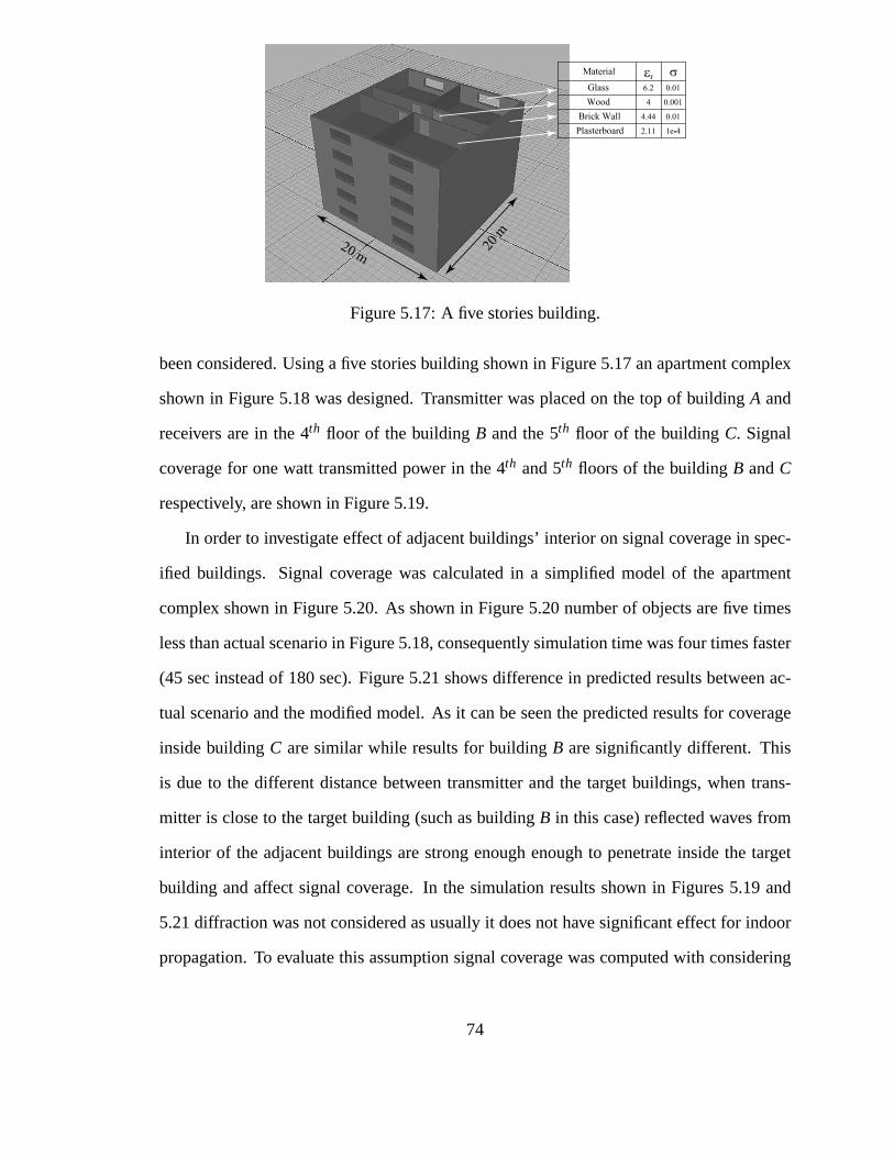
for two different car models (Tx at 1st floor). . . . . . . . . . . . . .. . . 725.16 Signal coverage inside the covered parking structure shown in Figure 5.13
for two different car models (Tx at 2nd floor). . . . . . . . . . . . . .. . . 735.17 A five stories building. . . . . . . . . . . . . . . . . . . . . . . . . . . .. 745.18 An apartment complex. . . . . . . . . . . . . . . . . . . . . . . . . . . . .755.19 Signal coverage inside buildingsB andC shown in the Figure 5.18. . . . . . 755.20 Simplified model of apartment complex shown in the Figure 5.18. . . . . . 765.21 Difference in signal coverage between actual and simplified models. . . . . 775.22 Difference in predicted signal coverage due to diffraction effect. . . . . . . 775.23 Relative error in predicted results vs. angular resolution. . . . . . . . . . . 785.24 Simulation time vs. angular resolution. . . . . . . . . . . . .. . . . . . . . 795.25 A typical suburban area. . . . . . . . . . . . . . . . . . . . . . . . . . .. 805.26 Predicted signal coverage without effect of terrain. .. . . . . . . . . . . . 805.27 Predicted signal coverage with effect of terrain. . . . .. . . . . . . . . . . 815.28 Flowchart of through wall imaging method. . . . . . . . . . . .. . . . . . 835.29 A typical scenario used in simulation. . . . . . . . . . . . . . .. . . . . . 845.30 Angle of arrival for the target at the 4th floor in B1. . . . . . . . . . . . . . 865.31 Angle of arrival for the target at the 5th floor in B2. . . . . . . . . . . . . . 865.32 Field map at the 4th floor in B1. . . . . . . . . . . . . . . . . . . . . . . . . 875.33 Field map at the 5th floor in B2. . . . . . . . . . . . . . . . . . . . . . . . . 885.34 Frequency response of focused power at target. . . . . . . .. . . . . . . . 885.35 Reduction in focused power due to frequency shift. . . . . .. . . . . . . . 895.36 Focused power is reduced by decreasing number of sensors. . . . . . . . . 896.1 Time domain response of the SPMS for a through case in the absence of
scatterers. . . . . . . . . . . . . . . . . . . . . . . . . . . . . . . . . . . . 916.2 Top view of a simplified scenario considered for measurement. . . . . . . . 936.3 Measured frequency response for different points on thereceiver path shown
in Figure 6.2. . . . . . . . . . . . . . . . . . . . . . . . . . . . . . . . . . 936.4 Measured and simulated pathloss for receiver path shownin Figure 6.2. . . 946.5 Top view of a scenario with five two stories building. . . . .. . . . . . . . 956.6 Measured frequency response for different points on thereceiver path shown
in Figure 6.5. . . . . . . . . . . . . . . . . . . . . . . . . . . . . . . . . . 956.7 Measured and simulated pathloss for receiver path shownin Figure 6.5. . . 966.8 Top view of a scenario with seven two stories building. . .. . . . . . . . . 966.9 Measured pathloss at different frequencies for receiver path shown in Fig-
ure 6.8. . . . . . . . . . . . . . . . . . . . . . . . . . . . . . . . . . . . . 976.10 Measured and simulated pathloss for receiver path shown in Figure 6.8. . . 97
ix
Page 11
6.11 Top view of a scenario with seven two stories building. .. . . . . . . . . . 986.12 Measured and simulated pathloss for receiver path shown in Figure 6.11. . . 996.13 Two independent pathloss measurement for scenario shown in Figure 6.11
shows the SPMS stability. . . . . . . . . . . . . . . . . . . . . . . . . . . . 99A.1 Multi-layer dielectric slab. . . . . . . . . . . . . . . . . . . . . . .. . . . 105B.1 Interdigital capacitor; (a) Layout, (b) Circuit model. . .. . . . . . . . . . . 109B.2 Wafer holder with a cavity under DUT. . . . . . . . . . . . . . . . . . .. . 110B.3 Series capacitance of interdigital capacitors in CPW lines. . . . . . . . . . 112B.4 Measured and simulated S-parameters of interdigital capacitor,L f = 100µm;
(a) Magnitude, (b) Phase. . . . . . . . . . . . . . . . . . . . . . . . . . . . 113B.5 Measured and simulated S-parameters of interdigital capacitor,L f = 250µm;
(a) Magnitude, (b) Phase. . . . . . . . . . . . . . . . . . . . . . . . . . . . 114B.6 Measured and simulated S-parameters of interdigital capacitor,L f = 300µm;
(a) Magnitude, (b) Phase. . . . . . . . . . . . . . . . . . . . . . . . . . . . 115B.7 Characterization of effective inductance and resistancefor short stubs in
CPW line; (a) Inductor layout, (b) Circuit model. . . . . . . . . . . .. . . 116B.8 Inductance of short circuit stubs in CPW lines. . . . . . . . . . .. . . . . . 116B.9 New inductive coupled resonator bandpass filter circuit model. . . . . . . . 116B.10 New inductive coupled resonator bandpass filter layout.. . . . . . . . . . . 118B.11 Simulation results for the new inductive coupled resonator bandpass filter
vs standard type of this filter. . . . . . . . . . . . . . . . . . . . . . . . . .118B.12 Simulation and measurement results for the new inductive coupled res-
onator bandpass filter. . . . . . . . . . . . . . . . . . . . . . . . . . . . . . 119B.13 Miniaturized highpass filter layout. . . . . . . . . . . . . . . . .. . . . . . 120B.14 Simulation and measurement results for the miniaturized highpass filter. . . 121
x
Page 12
LIST OF APPENDICES
AppendixA Coherent approach for calculating reflectivity from multi-layer dielectric
slabs . . . . . . . . . . . . . . . . . . . . . . . . . . . . . . . . . . . . . . 104B Characterization of semi-lumped CPW elements for mm-wave filter design 107
xi
Page 13
CHAPTER 1
Introduction
1.1 Motivation
Wireless systems have become prevalent for a wide range of commercial and military
applications. The third generation (3G) of wireless communications is currently being
developed and will reach full development by 2005. The 3G systems will provide multi-
media services and satisfy the desired “anytime and anywhere” requirement [1]. The 4G
systems which are currently being discussed [2] will provide an all-IP network that inte-
grates several services available at present and provides new ones, including broadcast,
cellular, cordless, wireless local area network (WLAN), andshort-range communication
systems. In future defense systems, the integration and interdependent operation of mil-
itary ground, surface, air, missile, and space-based radarand communication systems for
enhanced overall defense effectiveness will be very critical. Instead of autonomous plat-
forms, future collector systems, processors, and users will share information via networks.
During operations, the engagement systems will have the ability to reach back for informa-
tion that will enable them to provide more adaptable quick-reaction forward “footprints”
(presence). Ground forces will also contribute to the totalsituation awareness with im-
proved communications and sensor systems. Soldiers’ positions will be known accurately
via global positioning system (GPS) satellite receivers, and they will be able to access
1
Page 14
secure spread-spectrum cellular-like systems with voice and data links. Data from night-
vision, spectrum-scanning, and video sensors will be linked back to headquarters over cel-
lular systems or directly to satellites. Throughout the entire system configuration, many
images per second will be collected, processed, and the information shared in real time. In
addition to improved radar and communication capabilities, this environment will demand
significantly increased signal and information processingcapabilities [3]. Hence the gen-
eral trend in the development of future wireless communication is the use of higher data
rates (broader frequency band) and propagation in more complex environments.
One of the most critical aspects in designing a wireless system is the accurate character-
ization of the propagation channel. Accurate channel modelling in wireless communication
allows for: 1) improved system performance (bit error rate,battery life, etc.), 2) reduced
interference, to ensure proper operation of other commercial systems and provide secure
communication for military purposes.
Numerous methods and techniques have been developed to predict the effect of the
channel, and these can be divided to two categories: 1) Statistical or empirical models like
Okumara [4], Hata [5] and Longley-Rice [6], and 2) Deterministic or analytical models like
ray-tracing based models [7–12]. Statistical models are based on measured data. There-
fore to develop these models, many measurement data sets arerequired. A draw-back of
these empirical models is that they are only applicable to environments which have similar
geometry to the measurement bases. Therefore to build a general and accurate model an
exorbitantly large number of measurement sets are required.
Deterministic methods are based on the physics of the environment and wave prop-
agation phenomena such as reflection, transmission, and diffraction. These methods are
generally applicable to any arbitrary environment especially especially useful for micro-
and pico-cellular environments where statistical models fail. In these cases the wave prop-
agation phenomena is highly the site specific. One major taskin the development of de-
terministic models is to verify the accuracy of the predicted results. This can be done by
2
Page 15
careful measurements where besides the signal parameters,all physical details of the envi-
ronment are determined and ported to the simulator. In addition, dielectric properties of the
actual materials and their spatial variations must be measured and considered in the model,
where is practically very difficult if not impossible.
An alternate approach to the time consuming and expensive outdoor measurements is
the proposed scaled measurement system in this thesis. Thisallows accurate measurement
of well defined channels under a controlled laboratory environment. A millimeter-wave
scaled propagation measurement system (SPMS) is designed for this purpose. Confining
the desired range of frequency to systems operating at UHF toL-Band (0.5-2 GHz), dimen-
sions of scatterers and terrain features in the scaled propagation channel can be reduced by
a factor of 50-200 for the proposed SPMS that operates at around 100 GHz. This reduction
brings the size of building from few meters to few centimeters so a scaled model of city
block can easily fit in a laboratory, and measurements can be done quickly, accurately, and
cost effectively.
1.2 Background
In this section, first wireless channel models are reviewed.Then importance of propa-
gation measurement for developing or verifying of channel models and difficulties involved
in that are described. As W-band transceivers are major subsystems of the Scaled Model
Propagation System (SMPS), the second part of this chapter briefly introduces most recent
reported researches on W-band circuit modules and systems.
1.2.1 Wireless Channel Modelling
Developing propagation models for urban environment started as early as four decades
ago. These models were developed for VHF and UHF broadcasting, based on measured
data and few simple corrections factor such as frequency, antennas height and gain. Those
3
Page 16
models were able to provide a rough estimation about coverage or path-loss, which was
sufficient at that time because any inaccuracy in coverage estimation were compensated
by increasing transmitting power without a significant costincrease in the broadcasting
system. Growth of wireless communication made electromagnetic (EM) spectrum more
crowded and consequently more restricted spectrum regulation has been imposed by the
standard organization such as Federal Communications Commission (FCC). While these
standards ask for lower power transmission to minimize interference among systems, new
applications with higher bandwidth need higher signal to noise ratio (S/N) to provide ade-
quate bit error rate (BER). Hence every part of the wireless system needs to be optimized
at extreme levels including the channel.
In 1990’s theoretical and numerical channel models were proposed and still expanding
in order to accomplish channel modelling with higher accuracy and more details such as de-
lay spread, coherence bandwidth, and Doppler spread which are crucial for new digital and
mobile systems. Fortunately, at the same time new computerswith faster computational
speed have become available and helped developing these channel models. The theoreti-
cal models can be divided into two categories: 1) Physics-based models, and 2) Statistical
models. Although physics-based models are more accurate and take the environment de-
tails into account, their usage is still limited to micro- and pico-cellular scenarios which
statistical models cannot provide useful estimation. The main causes of this are difficulties
in importing the physical environment data, such as geometry, topography, and material
properties, and also lack of model verification by measurements. Hence communication
scientists still rely on statistical models which are developed based on measured data. In
what follows these two categories of channel models are briefly introduced and at the end
difficulties and errors involved in channel measurement which is required for both models
are reviewed.
4
Page 17
Measurement-based Statistical Models
Measurement-based models are developed based on extraction of statistical behavior of
channel from extensive measurements data. Okumura model [4] is one of the first empirical
channel models. This model can predicts path-loss only and takes into account some of the
propagation parameters such as the type of environment and the terrain irregularity. These
parameters are added to mean path-loss value which is found by few looking up curves. The
measurement based models have become more accurate and complicated by incorporating
environment details as much as possible [5,13] and it also has been tried to use these models
for indoor scenarios [14]. As mentioned earlier in order to develop an accurate statistical
model a comprehensive measurement data is required, which is certainly time consuming
and costly.
Site-Specific Models
Site-specific models are built up by considering the environment details, wave prop-
agation phenomena such as reflection and diffraction, and finding signal paths between
transmitter and receiver. Primary models in this category were based on simplistic situa-
tions and finding few paths such as direct, ground reflection,and rooftop diffraction [15].
Later with the advancement of computer capabilities, more complex channel simulators
were developed based on ray-tracing or image algorithms [7–12]. These models seems to
be the best candidates for providing all channel information required in optimizing the next
generation of communication systems. However the difficulties in importing environment
details to these simulators, lack of model verification by field measurements are the weak
points of these models that must be overcome.
Model Verification by Field Measurement
As described in last two subsections, field measurements is important either for devel-
oping channel models or verifying simulated result of a channel model. However outdoor
5
Page 18
measurements are expensive and time consuming [16,17]. Also there are many factors such
as traffic (cars, pedestrian, ...) which are not under control and affect the measurements.
Furthermore for site-specific models the discrepancies between the measurement site and
data used in simulation one can be significant, hence the verification process will end up
with large margins of error.
1.2.2 W-Band Transceivers Background
The SPMS operation frequency is chosen around 100 GHz which gives maximum scal-
ing ratio while transceivers’ circuits can be fully characterized using available lab equip-
ments. It will be described later that the SPMS works similarto standard millimeter-wave
(mm-wave)S21 measurement setup. This means vector network analyzer (VNA) signal
will be up- and down-converted to desired operation signal using two mm-wave modules.
However for a propagation measurement system, receiver andtransmitter probes are mo-
bile, consequently it is not possible to use available mm-wave modules. Moreover, the
probes’ size has to be small in comparison with scaled buildings to minimize its interac-
tion in the measurement environment. Hence design and fabrication of special receiver and
transmitter probes is required. As construction of W-band probes is a major part of this the-
sis, in this section a brief background of recent mm-wave circuit components and systems
are presented.
Subharmonic Mixers
High power signal generation at mm-wave frequencies is verydifficult, so a major
concern in mm-wave systems is loss reduction specially at frequency conversions which are
one of the most lossy part of a system. Hence mixers are one of the challenging components
in mm-wave systems. An alternative to direct conversion technique is using subharmonic
mixers. The subharmonic mixers are often used because it is easier and less expensive
to generate a high power, and low phase noise source at a subharmonic of required local
6
Page 19
Table 1.1: MM-wave subharmonic mixers performance comparisonRF Freq.(GHz) LO Freq.(GHz) Features, Pub. Ave. Conv. Loss(dB)
84-102 45 W.G.P1, [19] 11
92-96 45 Flip Chip, [20] 10
92-94 45 Flip Chip, [21] 8
112-120 62 MMIC2, [22] 16
230-240 120 MMIC, W.G.P, [23] 9.5
175-182 96 MMIC, W.G.P, [24] 16
154-170 77 Flip Chip, [25] 13
75-77 15.1 Flip Chip, [26] 23
80-110 48 MMIC, [27] 121Waveguide Package,2Monolithic Microwave Integrated Circuit
frequency.
Furthermore in order to have a coherent transceiver system common LO source must be
used for both transmitter and receiver, this means LO signalmust be carried in a long path
from its source to the mobile receiver. Clearly, carrying lower frequency signal (K-band)
in flexible coax cables can be done much easier than carrying aW-band signal through
waveguides.
The diode based subharmonic mixers are a major category of these mixers. Antiparallel
diode pair is a popular choice for subharmonic mixers becasue it creates a symmetricalV-
I characteristic that suppresses the fundamental mixing product of the RF (or IF) and LO
signals and leads to a better conversion loss [18]. Comparison between some of the reported
results of mm-wave subharmonic mixers are shown in table 1.1.
Filters
Subharmonic mixers generate undesired harmonics as well asdesired one because of
their nonlinear nature. Hence for a transceiver system it isvery important to weaken un-
desired spurious by filtering to have a single tone communication link. Also appropriate
7
Page 20
filtering at LO and IF ports of a mixer increase its efficiency.In this section a brief history
of planar mm-wave filters are reviewed. As coplanar waveguide (CPW) is the optimum
choice in terms of electromagnetic properties at mm-wave and simple fabrication most
reviewed papers in this section are CPW based filters.
Although microwave filters have been studied extensively but there are not many arti-
cles about planar mm-wave filters, specially at W-band. There are few difficulties involved
in filter design and fabrication at mm-wave and above. Most parasitic elements, that are
usually ignored at lower frequencies design procedure, have significant effect at mm-wave
frequencies. The parasitic elements and their effects cannot be considered as design param-
eters. Hence these effects have to be accurately modelled and compensated. Alternatively
use of structures with minimal parasitic effects should be considered. CPW line disconti-
nuities are well characterized at microwave frequencies [28–30] and are studied at higher
frequencies up to 50 GHz [31–33]. However modelling and characterization of such dis-
continuities at W-band frequencies is rather sparse and incomprehensive. Calibration ac-
curacy at W-band is one of the major difficulties for characterization parasitic capacitance
and inductors which are as small as fewf F ’s andpH’s respectively.
Table 1.2 shows important parameters for few filters in some of the recent reported
studies [34–38]. It should be noted fabrication process forall of these filters are not similar
consequently it is not possible to compare their performance clearly.
W-Band Systems
W-band systems are mainly designed for radar applications [39–41]. These radar or
transceiver MMIC’s are fabricated in the state of the art labssuch as TRW [40] with 0.1µm
fabrication technology which is not commercially available. In this thesis, design is done
using flip-chip elements in order to reduce fabrication costand make it feasible using the
University of Michigan clean room facilities.
8
Page 21
Table 1.2: Planar microwave filters performance comparisonF0 (GHz) BW (%) I.L. (dB) Order Rej.@ F0±BW (dB) Pub.
10 20 2.2 3 – [35]
10 10 3.4 3 – [35]
10 5 5.4 3 – [35]
20 35 2.2 3 22 [34]
30 53 2.5 3 13 [36]
65 22 1.5 3 13 [38]
83 36 1.8 3 17 [38]
92 5 4.2 3 – [38]
95 6.1 3.4 5 42 [37]
95 12.5 2.2 5 33 [37]
95 17.7 1.4 3 22 [37]
1.3 Thesis Framework
Figure 1.1 shows the main components of the W-band SPMS. The system includes an
x-y-z probe positioner, scaled model of a city block, miniaturized W-band transmitter and
receiver probes, and a vector network analyzer. The networkanalyzer in the SPMS is used
for signal processing and data acquisition. Therefore the setup is configured to characterize
the propagation channel in a manner similar to the standardS21 measurement. The network
analyzer allows for coherent and broadband path loss measurement with a wide dynamic
range. Also the time domain features of the network analyzerallow for measuring the
power delay profile which makes the SPMS unique in channel modelling. In order to move
the receiver probe with the required accuracy (to within a fraction of the wavelength∼= 3
mm) for measuring fast fading and slow fading statistics, a computer-controlled xy-table
has been designed and built. As the operating frequency of the network analyzer (L-band)
is different from the required SPMS frequency (W-band), an up- and down-converter has
been designed and fabricated as part of the transmitter and receiver probes respectively. To
minimize the interaction of the probes with their environment, they must be designed as
9
Page 22
VNA
X-Y- Z Table
Tx Probe
Scaled Model
LO
LO
IF
IF
Computer
Rx Probe
Figure 1.1: Scaled propagation measurement system block diagrams.
small as possible.
The design, fabrication, and performance of individual circuit elements of SPMS will
be demonstrated in chapter 2. Construction of scaled buildings and different techniques
used for characterization of building’s material are described in chapter 3. XY table, which
is an automatic positioner for receiver probe, and its specifications are also explained in this
chapter. The system calibration and overall system specifications are presented in chapter
4. Chapter 5 explains a physics based site specific channel model using 3D ray-tracing with
few examples for indoor, outdoor and suburban areas. Chapter6 demonstrates few sample
measurements of path-loss, coverage and power delay profile(PDP) and is also on model
verification by comparison between theory and measurement.Finally the conclusion of
this study and its applications and future work are introduced in last chapter (chapter 7).
Figures 1.2 and 1.3 show the thesis flowchart and percentage of each tasks and sub-tasks
respectively.
10
Page 23
Scaled Propagation Meas. System Design
MM-Wave &
RF SubsystemsScaled CityXY-Table
SoftwareHardwareMaterial
Dielectric Meas.
Building
Fabrication
LO & IF
Circuits
W-Band
Transceivers
System
Calibration
MeasurementPhysics based
Channel Simulation
Validation &
Model Improvement
Figure 1.2: Thesis flowchart.
0
20
40
60
80
100
Thesis Task
System Design
CircuitModules
XY-TableScaled
BuildingSystem
CalibrationMeasurement& Validation
Simulator
Des
ign
AD
esig
n B
1D
esig
n B
2
Des
ign
Fab
rica
tion
Tes
tP
acka
ging
Per
cent
age
(%)
Har
dw
are
Con
trol
ler
Sof
twar
e &
GU
I
Fab
rica
tion
Mat
eria
l C
hara
cter
izat
ion
Dia
gnost
icN
ew S
ub-S
yste
ms
Deb
ug &
Ext
ensi
on
for
New
App
lica
tion
Mea
sure
men
tV
alid
atio
n
Figure 1.3: Thesis tasks and sub-tasks.
11
Page 24
CHAPTER 2
Circuit Components
In this chapter design, fabrication, and performance of individual circuit elements in
the scaled propagation measurement system (SPMS) will be demonstrated. First part of
the chapter describes W-band transceiver probes and their sub-circuits and second part of
the chapter is on extra circuit modules designed for IF and LOsignals and overall system
performance improvement.
In the SPMS a stepped-frequency vector network analyzer (VNA) is used as the base
for coherent transceiver proposed system. As it is shown in Figure 2.1, the signal from
the VNA is up and down converted between the W- and L-bands by the transmitter and
receiver probes. Same LO source is used for transmitter and receiver probes which not
only allows for coherent measurement of the fields but also for measurement of very weak
signals by reduction of the network analyzer’s IF bandwidthto its minimum value (10 Hz
for HP8720D). Narrow IF bandwidth reduces the noise level and permits measuring signals
at very low power levels (around -110 dBm for HP8720D). To maintain the high fidelity of
the VNA signal The local signal source in the SPMS is generated by a dielectric resonator
oscillator that has a frequency variation of 6 kHz/0C and a phase noise of -86 dBc/Hz at 10
kHz offset from the center frequency. The common LO operatesat 23.7 GHz and drives the
subharmonic mixers in transmitter and receiver probes through a set of high quality flexible
coaxial cables.
12
Page 25
2-4 GHz, 5 to -85 dBmPort 2 VNA
2-4 GHz, -10 dBmPort 1 VNA
Hybrid~
W-BandTransmitter
IFAmplifier
Isolator
W-BandReceiver
LOFilter
LOFilter
IFAmplifier
Isolator
-55 to -145 dBm90.8-92.8 GHz
Scaled City
LOAmplifier
LOAmplifier
FIF
FIF
FLO
FLO
0 dBm
FRF 0 dBm90.8-92.8 GHz
-1.5 dBm
0 dBm
16 dBm
16 dBm
FRF
-55 to -145 dBm
23.7 GHz 3 dBm, DRO
Figure 2.1: SMPS circuit components diagram.
The VNA used in the SPMS (HP8720D) can provide up to 5 dBm of output power,
however the harmonics level at maximum output power are relatively high and adversely
affect the quality of the overall measurement. Hence the VNAoutput power is set at -10
dBm and an IF amplifier is used to produce sufficient power at theIF port of the transmitter
probe. Isolators are placed in order to improve matching andprevent signal ringing in
the cables. The LO amplifiers are narrow-band and have significant rejection at IF band.
In addition narrow-band filters are designed and placed at the LO ports to increase the
isolation between the IF ports of the transmitter and receiver probes. This prevents the IF
signal leakage through direct path between the transmit andreceive ports of the VNA.
The simulation results in the following sections were performed by ADS Momen-
tum for the passive elements, and a harmonic balance simulator for nonlinear analysis
of the subharmonic mixer. The measurement were realized using a probe station (for on
wafer measurements), HP-8510C network analyzer, HP-W85104A mm-wave test setup,
HP-8562A spectrum analyzer, and HP-11970W waveguide harmonic mixer.
13
Page 26
Subh armonic Mixer
RF Filter
Amplifier Antennas
FRF
Subh armoni c Mixer
RF Filter
Amplifier Antennas
IF Port2-4 GHz
IFFilter
IFFilter
mFLO
RF Signal
90.8-92.8 GHz
nFIF
mFLO nFRF
FRF = 4FLO - FIF
23.7 GHz
IF Port2-4 GHz
LO Port
LO Port
Figure 2.2: W-band transmitter and receiver probes block diagrams.
2.1 W-Band Transceivers Probes
Figure 2.2 shows the block diagrams of the transmitter and receiver probes. As shown in
the upper branch, the IF signal (FIF ) from the output of the network analyzer is mixed with
the local oscillator signal (FLO) in a subharmonic mixer to generate the transmitter signal.
This signal contains all harmonics of the formmFLO±nFIF . The desired harmonic, which
results from mixing the 4th harmonic of the LO signal and the IF signal, is selected by
the RF filter for transmission. Then it is amplified and transmitted. At the receiver (lower
branch in Figure 2.2), the RF signal captured by the antenna isamplified before down-
conversion at the receiver subharmonic mixer. Then the desired IF signal (4FLO−FRF) is
selected by the IF filter and delivered to port 2 of the networkanalyzer after IF amplifica-
tion (not shown). Subharmonic mixers are used to allow for stepped frequency operation
without need for distributing a common W-band local oscillator to mobile transmitter and
receiver probes, which is practically impossible. The transceiver circuit was fabricated on
a 10 mils (∼= 250µm) thick quartz wafer. As the width of a 50Ω microstrip line on avail-
able substrates becomes comparable with the wavelength at W-band frequencies, microstrip
lines become inappropriate for circuit design. Also to be compatible with the test setup,
14
Page 27
InterdigitalCapacitor
10 µ
m
60 µ
m
0.7 mm
IF RF
Figure 2.3: IF filter layout and dimensions.
the circuit was designed and fabricated using CPW lines. The fabrication processes were
performed in the University of Michigan’s clean room, usingthe wet-etching technique on
3 µm electroplated gold on the quartz wafer. The skin depth for the RF, LO, and IF frequen-
cies are 0.26, 0.52, and 1.5µm respectively. The gold thickness is marginally sufficientfor
the IF signal, but as it will be shown, the minimum feature size in the circuits is 10µm,
which limits the thickness of the plated gold that can be used. Fortunately insufficient metal
thickness does not degrade the circuit performance becausein this miniaturized circuit the
IF signal path on the circuit is just 2.5 mm which is smaller than 0.01λIFg . Therefore the
associated metallic loss is negligible.
2.1.1 IF Filter
The IF filter is placed to isolate the IF and RF signals in order to improve the sub-
harmonic mixer’s efficiency. There are many topologies thatcan be used for this filter.
However to minimize the size, a low pass filter constructed from a quarter wavelength high
15
Page 28
S21
(dB
)
-10
-5
0
-15
S11
(dB
)
-20
-10
0
-30
Simulation Mesurement
Frequency (GHz)0 25 50 75 100
Figure 2.4: Simulation and measurement results for IF filter.
impedance line terminated by an inter-digital capacitor isused. For this simple filter the
higher is the capacitance and the line impedance, the lower is the RF signal leakage to the
IF port. Hence the aim is to increase the capacitance and the line impedance as much as
possible. However these two parameters are limited by the minimum achievable feature
size in the fabrication process, which is about 10µm. Figure 2.3 shows the IF filter layout.
For the specified dimensions in this figure, a line impedance of 145Ω and an interdigital
capacitance of 75 fF with a quality factor of 10 at the W-band are achieved. The MoM
simulation and the measured transmission coefficient and return loss for the IF filter are
plotted in Figure 2.4, where excellent agreement is shown. There are no measured data
between 40-75 GHz. The maximum insertion loss of this filter at the IF signal is less than
0.1 dB, and its return loss is less than -24 dB over the desired IF frequency range. The
isolation between the RF and IF signals is more than 12 dB.
16
Page 29
0.55 mm
0.2
mm
10
µm
GND
GND
Figure 2.5: CPW coupled line for the first stage of RF filter.
2.1.2 RF Filter
The RF filter is intended for selecting the desired harmonic ofthe mixed IF and LO
signals (4FLO−FIF ) generated by the subharmonic mixer. It also prevents IF signal leakage
to the RF port which improves the conversion loss of the subharmonic mixer used for up-
and down-conversion. However, in the transmitter probe, inaddition to RF-IF isolation,
this filter should reject strong and undesired harmonics like the third and fifth harmonics of
the local oscillator to keep the RF amplifier from saturation.Furthermore, for single tone
transmission upper side band (USB) of up-converted IF signal(4FLO +FIF ) also has to be
attenuated sufficiently. In order to achieve all of the abovementioned features, the RF filter
is made of two cascaded band pass filters.
First Stage
A CPW coupled line filter shown in Figure 2.5 is selected as the first stage of the
RF filter. The advantages of this filter are high isolation between the RF and IF signal,
low insertion loss at the RF frequency range, compact size, and high impedance at the IF
frequency. Figure 2.6 shows the simulated and measured S11 and S21 of this filter as a
function of frequency. As can be seen, this filter provides more than 50 dB of IF to RF
isolation and has an insertion loss of less than 0.5 dB and a return loss of less than -25 dB
at the RF frequency range.
17
Page 30
S21
(dB
)
-40
-20
0
-60
S11
(dB
)
-20
-10
0
-30
Simulation Mesurement
Frequency (GHz)0 25 50 75 100
Figure 2.6: Simulation and measurement results for the CPW coupled line filter.
L0 L1 L0
−φ1−φ0−φ0−φ0−φ0
−φ1λ/2 λ/2
Figure 2.7: Circuit model of inductive coupled resonator filter for second stage of RF filter.
Second Stage
In order to generate a spurious free RF signal and also preventsaturation of the RF
amplifier by the undesired strong LO harmonics (3FLO at 71.1 GHz and 5FLO at 118.5
GHz), created by the subharmonic mixer, a second stage of RF filter is designed. The
second stage is constructed from two section inductively coupled resonators [42,43], whose
circuit model and topology are, respectively, shown in Figure 2.7 and 2.9. The inductive
coupling between the resonators is achieved by symmetric short circuited CPW line stubs
as shown in Figure 2.8(a). A simple method to calculate the inductance of these stubs is
the classical formula for ribbon inductors [42].
18
Page 31
w
l
(a)
L
R
Ζ0, φ0Ζ0, φ0
(b)
Figure 2.8: Characterization of effective inductance and resistance for short stubs in CPWline; (a) Inductor layout, (b) Circuit model.
Table 2.1: Effective Inductance of Short Stubs in CPW LineInductor# w(µm) l(µm) MoM (pH) Eq. 2.1 (pH)
1 60 20 5.1 1.4
2 30 20 7.1 1.8
3 30 136 21.1 32.9
4 30 198 25.0 54.9
5 25 213 33.0 64.3
L = 2lln(2πl/w)−1+w/πl nH (2.1)
wherew and l (in cm), are the width and length of the inductor, respectively. However,
the accuracy of this formula is quite poor with errors often greater than 100%. Therefore
to extract an accurate effective inductance of these short stubs, the MoM simulated S-
parameters of the stubs, shown in Figure 2.8(a), are compared with its circuit model, shown
in Figure 2.8(b). Table 2.1 shows the calculated inductances using (2.1) and the extracted
values from the MoM simulation. The MoM results are used in the final design, and as
will be shown, they lead to excellent agreement between the measured and simulated filter
responses. In order to provide the required out-of-band rejection and minimum insertion
loss simultaneously, a 2-pole filter is found to be the optimum choice. The design of this
19
Page 32
1.9 mm
0.7 mm
30 µm
Figure 2.9: Photograph of fabricated inductive coupled resonator filter on Quartz wafer.
filter began with the corresponding lowpass element values,g0 . . .gn. Then using (2.2, 2.3,
and 2.4),L j(Xj/ω0) andφ j are calculated [42].
Z0/Xj =
(Z0
S)1/2− (
SZ0
)1/2 j = 1,n+1
Z0
S
√g j−1g j
g0g1− S
Z0
g0g1√g j−1g j
j = 2,3, . . . ,n(2.2)
S=πZT
2gog1
ω2−ω1
ω0(2.3)
φ j = tan−1 2Xj
Z0(2.4)
whereZT andZ0 are the characteristic impedance of the CPW line and port impedances
respectively. In this design both are chosen to be 50Ω. In (3) ω0,ω1, andω2 are the center,
lower cut-off, and higher cut-off angular frequencies. A photograph of the fabricated filter
is shown in Figure 2.9. Figure 2.10 shows the simulated and measured filter responses.
Magnetic current concept is used in the MoM simulation for fast computation and more
accurate excitation of CPW structures. As such, conductive loss is not modelled. This
effect was considered in simulation by extracting inductors and CPW line parameters from
measured results and used in the simulations. Figure 2.10 shows filter rejection at 3FLO
and 5FLO to be more than 35 dB. Also the closest undesired harmonic to the RF signal,
which is the upper side-band of the up-converted IF signal (4FLO +FIF = 96.8-98.8 GHz),
20
Page 33
-20
-10
S21
(dB
)
0
-40
S11
(dB
)
-20
-10
0
-25
Frequency (GHz)75 85 95 105
Simulation Mesurement
-30
-5
-15
Figure 2.10: Simulation and measurement results for the inductive coupled resonator filter.
is at least 30 dB attenuated through two such filters at the transmitter and receiver probes
totally. This ensures that the SPMS is able to measure fadingdepth at least as low as
30 dB. In extension of filter design, using shunt inductive stubs introduced in this section
and interdigital capacitors a novel bandpass filter and a miniaturized highpass filter were
designed and fabricated. Details are presented in appendixB.
2.1.3 Subharmonic Mixer
The conversion loss and noise performance of a millimeter-wave mixer usually is lim-
ited by insufficient LO power or by excessive LO noise [44]. Generally mixers are pumped
at half or a quarter of the required LO frequency. The major disadvantage of this technique
is a higher conversion loss compared to fundamental mixers.Considering the transmitter
probe’s block diagrams, the extra conversion loss of the subharmonic mixer is tolerable
as long as the up-converted signal power reaches to the minimum input power to achieve
maximum, distortion free, output power of the RF amplifier, which in this case is -24 dBm.
21
Page 34
Table 2.2: GaAs Schottky Diodes CharacteristicsRs (Ω) Rj (Ω) Cjo (fF) CT (fF) VF (V) VBR (V)
MACOM 4 2.6 20 45 0.7 7.0
Alpha 7 4 35 55 0.7 3.0
An antiparallel diode pair is a common choice for subharmonic mixers. The reason is
the symmetrical V-I characteristic of the antiparallel diodes that suppresses the fundamental
and even harmonics mixing product of the LO and RF (or IF) signal. It should be noted that
proper operation of the subharmonic mixer depends on the similarity of the two back-to-
back diodes. In our design we have used a GaAs flip chip schottky antiparallel diode pair
manufactured by MACOM and Alpha Industries Inc. The specifications of these diodes are
given in Table 2.2. In order to improve the conversion loss ofthe mixer, the mixing product
near the second harmonic of the LO signal must be reactively terminated. Therefore, two
quarter-wavelength open stubs centered atF0 = FRF−2FLO are placed at both sides of the
antiparallel diodes to suppress the associated harmonics with the second harmonic of the
LO signal. As mentioned earlier, the RF and IF filters prevent IF and RF signal leakage
to the RF and IF ports respectively. A quarter-wavelength short stub at the LO frequency,
which acts as an open circuit for the LO signal and a short circuit for the IF and RF (FRF∼=
4FLO) signals, is also placed at the LO side of the subharmonic mixer to block IF and
RF signals leakage to the LO port. The subharmonic mixer circuit is optimized for the
best conversion loss, large signal matching at all ports, and minimum size. Figure 2.11
shows the subharmonic mixer layout with the IF and the first stage of the RF filters. Wire
bonds are placed at all discontinuities to suppress undesired slot modes on the CPW line.
The simulation and measured output RF power of the up-converter and conversion loss are
shown in Figures 2.12 and 2.13 respectively. As can be seen, the maximum up-converted
signal power is sufficient to provide the RF amplifier with the required input power for
maximum output. The maximum spurious level of the RF signal inthe SMPS is shown in
Figure 2.14, where it is shown that the average maximum spurious level is -40dBc. This
22
Page 35
Antiparallel Diodes
λ/4 @ FRF
−2FLO
λ/4 @ FRF
-2FLO λ/4 @ F
LO
IF Port
LO Port Wire
Bounds
RF
Port
2.4 mm
2.6 mm
Figure 2.11: Subharmonic mixer layout with IF and part of RF filters.
23
Page 36
MeasurementSimulation
-20 -10 0 10-50
-40
-30
-20
IF Power (dBm)
RF
Pow
er (
dBm
)FRF = 92.4 GHz, FLO = 23.7 GHz
PLO = 16.5 dBm
Figure 2.12: Simulated and measured RF power at the up-converter output.
allows for measurement of fading depths as low as 40 dB. The down-converter used in
the receiver probe has the same topology as the up-convertedwith similar performance
characteristics.
2.1.4 RF Amplifier
In order to compensate for the conversion losses of the up- and down-converter a W-
band amplifier is used in each probe. The amplifier chip is mounted on the circuit using
silver-epoxy. As shown in Figure 2.15 the input and output ofthe chip and DC contacts
are connected to the circuit using gold wire bonds. In the desired RF frequency range the
amplifier has a gain of 27-29 dB and a noise figure of 4 dB. Figure 2.16 shows the amplifier
gain, noise figure, and its input and output return losses.
24
Page 37
2 2.5 3 3.5 420
25
30
35
40
IF Frequency (GHz)
Co
nv
ersi
on
Lo
ss (
dB
)
MeasurementSimulation
PIF = -6 dBm, PLO = 16.5 dBm
FLO = 23.7 GHz
Figure 2.13: Simulated and measured conversion loss of the up-converter.
RF Frequency (GHz)
MeasurementSimulation
91 91.5 92 92.5-60
-50
-40
-30
-20
Max
Spu
riou
s L
evel
(dB
c)
Figure 2.14: Simulated and measured spurious level of the RF signal in SPMS.
25
Page 38
Figure 2.15: Photograph of RF amplifier and its wire bonded connections to the circuit.
Gai
n &
NF
(dB
)
10
20
30
0
Ret
urn
Los
s (d
B)
-20
-10
0
-30
Frequency (GHz)75 85 9580 90 100
NFGain
Input R.L.Output R.L.
Figure 2.16: RF amplifier gain, noise figure, input and output return loss.
26
Page 39
S1
1 (
dB)
-10
0
-15
Frequency (GHz)75 85 95 105
w/o Matching w/ Matching
-5
Figure 2.17: Effect of matching line on antenna return loss.
2.1.5 Antennas
The main goal of the millimeter wave scaled measurement system is to characterize
propagation channels under laboratory conditions. In order to accomplish this properly,
the transmit and receive antennas should have broad beam patterns. A monopole antenna
is chosen for this purpose. As the monopole above a finite ground surface of the package
is not automatically matched, a quarter wavelength transmission line is used to match the
antenna to the circuit. As shown in Figure 2.17, quarter wavelength matching line has
improved antenna return loss about 5 dB at desired frequencyrange. Figure 2.18 shows the
antenna and the matching line between the antenna and the RF amplifier. The simulated
gain patterns of this antenna, above the packaged circuit, at E- and H-planes are shown in
Figures 2.19(a) and 2.19(b) respectively.
2.1.6 Packaging
The required accuracy in package dimensions has to be of the same order of the circuit
elements that are connected to the package. For example in a W-band system, an error as
27
Page 40
480 µm
z
x
10 µm
Figure 2.18: Photograph of monopole antenna and matching line.
90
60
30-30
-60
-120
-150
180
150
120
-15.0
-5.0
5.0
φ = π/2
θ
-90
(a)
90
60
30330
300
270
240
210
180
150
120
-5.0
5.0
-15.0
θ = π/2
φ
(b)
Figure 2.19: Simulated gain pattern of monopole antenna above packaged circuit; (a) E-plane, (b) H-plane.
28
Page 41
+1.5v dc for RF amplifier bias
LO port
IF port
Antennas
Figure 2.20: Packaged RF probe against a Quarter.
small as 10µm in the antenna’s position can change its resonant frequency by approxi-
mately 2 GHz and cause mismatching. A metallic package is designed using AutoCAD. In
order to achieve the desired accuracy, the package was milled at the University of Michi-
gan space research machine shop, using a high precision CNC machine with tolerances
less than 2.5 m. The fabricated circuit on the quartz substrate was diced using an automatic
dicing saw and then together with 2.4 mm coaxial connectors for the IF and LO ports was
assembled with the aluminum package. The LO and IF 2.4 mm connector pins are con-
nected to the circuit using silver epoxy. Figure 2.20 shows the packaged probe against a
Quarter.
2.2 LO and IF Circuit Modules
As it is shown in Figure 2.1 there are few circuit blocks otherthan W-band transceiver
probes. Some of these blocks have been purchased and only their specification will be
29
Page 42
mentioned in the next subsection however others have been designed and fabricated and
will be described in more details.
2.2.1 IF and LO Amplifiers
IF Amplifiers
IF amplifiers are placed at both transmit and receive paths. As mentioned earlier the IF
amplifier at transmit path is placed for helping VNA to operate at lower output power and
consequently reducing harmonic level [45]. In the receiverpath, the IF amplifier boosts
down-converted signal to be detectable by the port 2 of the VNA. The transmit path’s IF
amplifier gain and output power is obtained by optimum required IF power by W-band
transmitter probe (8 to 10 dBm) and its difference with minimum output power of the VNA
without using any internal attenuators (-10 dBm). Because using internal attenuators at
the VNA decreases its output signal to noise ratio (S/N). A double stage amplifier using
SiGe HBT RFIC manufactured byStanford Microdevices(SGA-5263) is fabricated for
this purpose. As the RFIC gain was not flat over IF frequency range two parallel RC are
places in cascade with each chip as gain equalizer. Figure 2.21 shows the packaged circuit.
Measured gain of this amplifier with and without gain equalizer is shown in Figure 2.22.
In receive path two high gain, low noise amplifier manufactured byMiteq is used which
provide 60 dB gain and has a noise figure of 2 dB.
LO Amplifiers
Two K-band amplifiers manufactured byNEXTEC-RFare used to amplify LO source
signal for W-band probes. These amplifiers have 20 dB gain andcan provide up to 20 dBm
output power. Because of the LO filter and cable losses, available power at LO port of
W-band probes is 16 dBm which is sufficient for proper operation of subharmonic mixer
inside the probes.
30
Page 43
RC Equalizers
Amplifier Chips
Figure 2.21: IF amplifier packaged circuit.
Gai
n (
dB)
20
25
15
w/o Equalizer w/ Equalizer
Frequency (GHz)2 2.5 3 3.5 4
Figure 2.22: IF amplifier gain with and without equalizer.
31
Page 44
IN
Tx Rx
Figure 2.23: Quadrature hybrid against a Quarter.
2.2.2 LO Source, Hybrid, and Filters
A 23.7 GHz dielectric resonator oscillator (DRO) built byLucix corporationthat has
a frequency variation of 6 kHz/0C and a phase noise of -86 dBc/Hz at 10 kHz offset from
the center frequency is used as common local source for transmitter and receiver probes.
The output signal of the DRO is distributed to the LO amplifiers by a quadrature hybrid.
The hybrid is not symmetric in order to compensate the difference between receiver and
transmitter cable losses and provide equal power for the probes. Figure 2.23 shows the
fabricated quadrature hybrid against a Quarter. Simulation and measurement results for this
hybrid are shown in Figure 2.24. Part of difference between measurement and simulation
is because of using a SMA load at the isolation port of the hybrid, which has reasonable
result up to 18 GHz. IF signal leakage from the transmitter tothe receiver probe through
LO path has to be kept lower than minimum detectable signal bythe receiver probe (-145
dBm). The LO amplifiers are narrow-band amplifiers and providetotal attenuation of 97
dB at this path for IF signal (S21@FIF = -37 dB,S12@FIF = -60 dB) however considering
IF signal level at transmitter probe (10 dBm) and IF to LO isolation at each probe (∼= 15
32
Page 45
S21
& S
31(d
B)
-10
-5
0
-15
S22
& S
33 (
dB)
-20
-10
0
-30
Simulation Mesurement
Frequency (GHz)23 23.5 24 24.5
Figure 2.24: Simulation and measurement results for quadrature hybrid.
2 12 22 27 32-80
-60
-40
-20
0
Frequency (GHz)
S2
1 (
dB
)
MeasurementSimulation
7 17
Figure 2.25: Simulation and measurement results for LO bandpass filter.
33
Page 46
Output BPF Input Matching
&Stubs
Gate biasDrain bias
LP6836P70
Figure 2.26: Frequency multiplier packaged circuit.
dB) still 30 dB more isolation is required. For this purpose aninductive coupled resonator
bandpass filter is added after each LO amplifier. These are 2-poles filter and each one
as shown in Figure 2.25 provide at least 60 dB attenuation at IF frequency band. It may
seems to be over designed however because of other coupling mechanism between circuit
modules using these filters found to be necessary.
2.2.3 Frequency Multiplier
In a primary system design it was intended to use a combination of a DRO operating at
one third of the desired local frequency and a frequency tripler to generate the LO signal
for W-band probes. For this purpose a frequency tripler weredesigned and fabricated. The
nonlinear element in the frequency tripler was a PHEMT builtby Filtronic (LP6836P70).
Figure 2.26 shows the fabricated circuit. The measured and simulated output power versus
input power and input frequency are shown in Figures 2.27 and2.28 respectively. It should
be mentioned that primary system design were based on a LO at 22.5 GHz.
34
Page 47
Pin (dBm)
MeasurementSimulation
0 5 10-35
-25
-15
5
15
Pou
t (dB
m) -5
Fin = 7.5 GHz
Figure 2.27: Output power vs. input power of the frequency multiplier.
Input Frequency (GHz)
MeasurementSimulation
7.1 7.3 7.5 7.7-10
-5
0
5
Pout
(dB
m)
Pin = 8 dBm
Figure 2.28: Output power vs. input frequency of the frequency multiplier.
35
Page 48
CHAPTER 3
Scaled Environment
In this chapter we discuss the construction process of scaled buildings followed by
different dielectric measurement techniques which were used for characterizing buildings’
material properties. Design, fabrication and specification of XY-table, which is a computer
controlled tool for precise placement and movement of the receive probe in the scaled city
is describe at the end of this chapter.
3.1 Scaled Building Fabrication
As mentioned earlier SPMS is designed to evaluate the performance of physics-based
propagation models. As such, beside electronic precision for signal amplitude and phase
measurement over a wide dynamic range, accurate rendition of the environment is also
important. This includes accurate knowledge of geometrical features of scatterers (like
buildings) as well as their material properties. To accommodate these features, scaled
buildings and other scatterers with an arbitrary degree of complexity and well-characterized
dielectric properties are used. A precise 3-D printer is used to make scaled buildings. The
3D printers use a powder-binder technology to create parts directly from digital data. First,
the 3D printer spreads a thin layer of powder. Second, an ink-jet print head prints a binder in
the cross-section of the part being created. Next, the buildpiston drops down, making room
36
Page 49
(a)
9 cm
12 cm
(b)
Figure 3.1: Scaled building; (a) CAD model, (b) printed building.
for the next layer, and the process is repeated. Once the partis finished, it is surrounded and
supported by loose powder, which is then shaken loose from the finished part. This printer
can use different materials and can make any building with any desired fine features. Any
standard CAD software can be used to draw the buildings and export the geometry file
for the 3D printer. Figures 3.1(a) and 3.1 show the CAD model ofa scaled building and
actual building printed by the 3D printer. Figure 3.2 shows the first version of a scaled city
block with simple building structures. It can be seen that the scaled city has a flexible grid
which is designed to help making an arbitrary arrangement ofthe blocks including roads,
sidewalks, cars, and buildings. The 3-D printer is capable of making complex building
with fine details such as one shown in Figure 3.3 and this feature can be used for maing
buildings with different level of details and study their effect on wireless channel using the
SPMS. The result of such study is very beneficial for physics-based model developments
as it helps to understand how important are the environment details and in what degree they
have to be considered in channel simulations.
3.2 Dielectric Characterization
Dielectric properties of scatterers are needed for numerical simulation of wave prop-
agation. Hence the material used to make the blocks must be characterized at W-band
37
Page 50
A Pen
Figure 3.2: Scaled city block.
(a) (b)
Figure 3.3: Scaled University of Michigan president building; (a) front view, (b) side view.
38
Page 51
frequencies. In this study, different techniques are used to characterize the real and imagi-
nary parts of the dielectric constant of the material used inconstructing the scaled buildings
over a wide range of frequency. The first method is based on capacitor measurements at
L-band and below and has been done using Agilent E4491A RF impedance/material an-
alyzer. The second method is based on transmission and reflection measurements in a
WR-90 X-band waveguide and post processing has been done usingHP 85071E mate-
rial measurement software. The third dielectric measurement is done at the W-band using
transmission measurement through a dielectric slab at different incidence angles, and re-
flection measurement of the back metal dielectric slab [46].The lower frequency dielectric
measurements are mainly done to verify the measured resultsat the W-band.
3.2.1 L-Band Measurement
For the L-Band measurements, an Agilent E4991A RF impedance/material analyzer
is used for characterizing the permittivity and loss tangent from 1 MHz to 3 GHz. The
dielectric samples used for this measurements are shown in Figure 3.4. The permittivity
and loss tangent measurement accuracy using this method arecalculated by applying 3.1
and 3.2 [47]:
∆εrm
εrm= ±
5+
(
10+0.1f
)
tεrm
+0.25εrm
t+
100∣
∣
∣
∣
1−(
13f√
εrm
)2∣
∣
∣
∣
[%] (3.1)
∆ tanδm
tanδm= ±[Ea +Eb][%] (3.2)
where,
Ea = 0.002+0.001
f· t
εrm+0.004f +
0.1∣
∣
∣
∣
1−(
13f√
εrm
)2∣
∣
∣
∣
(3.3)
Eb =
(
∆εrm
εrm· 1100
+ εrm0.002
t
)
tanδm (3.4)
39
Page 52
WR-90
X-Band Measured
Samples L-Band Measured
Samples
Figure 3.4: Dielectric samples.
f is the measurement frequency in GHz,t is thickness of the material under test (MUT)
in mm, εrm is the measured value of permittivity, and tanδm is the measured value of loss
tangent. For the measured samples with 1-2 mm thickness and typical permittivity of 3,
maximum error is approximately %10 at 300 MHz [47].Figure 3.5 shows measured per-
mittivity and loss tangent for two different samples.
3.2.2 X-Band Measurement
Dielectric characterization at X-band (8.2-12.4 GHz) is done using a transmission mea-
surement through cubic samples shown in Figure 3.4 in a WR-90 waveguide. HP 85071E
material measurement software is used for calibration and extracting the permittivity and
loss tangent from measured data. The transmission line method works best for materials
that can be precisely machined to fit inside the sample holder. The 85071E features an
algorithm that corrects for the effects of an air gap betweenthe sample and holder, consid-
erably reducing the largest source of error with the transmission line technique. The overall
accuracy of this technique is 1 to 2 percent [48]. Figure 3.6 shows measured results for two
40
Page 53
Lo
ss t
ang
ent
0.04
0.08
0.1
0
Per
mit
tiv
ity
2
2.5
3.5
1.5
Frequency (GHz)0 10.5 1.5 2
Sample 2Sample 1
3
0.02
0.06
Figure 3.5: Measured permittivity and loss tangent at L-band for two samples.
different samples using this technique.
3.2.3 W-Band Measurement
Figure 3.7 shows the free space measurement setup used for dielectric characterization
at W-band. The dielectric slab is placed in the far-filed of both horn antennas and is se-
lected large enough to minimize diffraction effects. Measurements for both transmission
through dielectric slab and reflection from a back metal slabmeasurement were performed.
However the reflectivity measurement showed better agreement with theory and is used as
final data. Calibration error, which can be seen as a fast variation in raw measured data, has
been removed using a 14th order lowpass Butterworth filter whose response in the spatial
domain, is shown in Figure 3.8. Measured reflectivity in the spatial domain before and
after filtering is shown in Figure 3.9. Coherent reflectivity for the back metal slab is calcu-
lated using the formulation in chapter 4.14 of [46] (see appendix A). Figures 3.10 and 3.11
compare simulated results for optimum values ofεr with measurement for two different di-
41
Page 54
Los
s ta
ngen
t
0.04
0.08
0.1
0
Per
mit
tivi
ty
2
2.5
3.5
1.5
Frequency (GHz)9 1110 12
Sample 2Sample 1
3
0.02
0.06
Figure 3.6: Measured permittivity and loss tangent at X-band for two different samples.
Dielectric Slab
WR-10 Horn
Antenna
WR-10 Horn
Antenna
Figure 3.7: Free space dielectric measurement setup at W-band.
42
Page 55
Distance (cm)
ButterworthElliptic
50 100-100
-75
-50
-25
0
S21
(d
B)
150
Chebyshev
Figure 3.8: Spatial domain filters.
Table 3.1: Measured Effective Dielectric ConstantFrequency Band L X W
Sample 1 2.7-j0.05 2.40-j0.04 2.34-j0.03
Sample 2 3.05-j0.15 2.70-j0.07 2.48-j0.06
electric slabs. The measurement results for the two different samples, using the discussed
techniques for different frequencies, are summarized in Table 3.1. The permittivity of ma-
terial used in the construction of the scaled buildings resembles those of brick and concrete.
3.3 XY Table
A computer-controlled xy-table that places the receiver probe at any arbitrary position
within a 1.5 m× 1.5 m area was designed and built. The system includes a motion control
card, two step-motors, power amplifiers, encoder and drivers. The computer issues com-
mands to the motion control card, which in turn triggers the power amplifier to drive the
43
Page 56
Distance (cm)
Filtered dataRaw data
50 150 250-40
-30
-20
-10
0
No
rmal
ized
Ref
lect
ivit
y (
dB
)
350
Figure 3.9: Measured reflectivity in the spatial domain.
Frequency (GHz)
MeasurementSimulation
80 90 100-45
-35
-25
-15
Ref
lect
ivit
y (d
B)
110
Un-filtered measured dataSlab Thickness: 1.2 cm
e'r = 2.34, e''
r = 0.03
Figure 3.10: Simulated and measured reflectivity of the dielectric slab at W-band, sample1.
44
Page 57
Frequency (GHz)
MeasurementSimulation
80 90 100-45
-35
-25
-15
Ref
lect
ivit
y (
dB
)
110
Un-filtered measured data
Slab Thickness: 1.1 cme'r = 2.48, e''r = 0.06
Figure 3.11: Simulated and measured reflectivity of the dielectric slab at W-band, sample2.
motor. An optical encoder attached to each motor sends the position and velocity data back
to the computer. The computer uses this information to control the probe movement. The
system placement is accurate to within 0.25 mm. This is acceptable accuracy even for fast
fading measurements at the RF frequency range (90.8-92.8 GHz) at which the wavelength
is about 3.3 mm. Figure 3.12 shows the block diagram of the xy-table system. A four layer
pcb (printed circuit board) with low interference considerations is designed and fabricated
for use as the motherboard of this system. Figure 3.13 shows the layout of this board.
45
Page 58
Computer With MotionControl Card
CommandSignals
EncoderDriver
OpticalEncoder Servo
Motor
Motion Control PWMServo Amplifier
DC Supply
Position and Velocity
Feedbacks
Axis
Figure 3.12: XY-Table block diagram.
X-axis
encoder
Y-axis
encoder
Z-axis
encoder
(optional)
X, Y
, Z ax
is
limit sw
itches
Motional control card
connector
Axis differential voltagesPower amplifier
Figure 3.13: XY-Table motherboard layout.
46
Page 59
CHAPTER 4
System Calibration and Specification
4.1 System Calibration
In the previous chapter the millimeter-wave scale measurement system and its major
components for the characterization of propagation environment were described. Through
the proper up- and down-conversion a vector network analyzer is used to presume the
amplitude and phase of the signal over a 2GHzbandwidth. Like any measurement instru-
ment, accurate measurements of field quantities in a propagation environment are limited
by measurement errors. The source of measurement errors canbe categorized into two
major groups.
1 Random errors that are not repeatable (uncorrectable) such as: a) thermal noise, b)
environmental changes, c) inconsistencies in attaching connectors, and d) operator error
2 Systematic errors that are repeatable (correctable) such as: a) mismatches at con-
nectors, b) leakage in directional couplers, c) differencein the system transfer functions of
different channels, and d) cross-talk between the reference and test channels. In this sec-
tion a brief discussion on the systematic error sources in the SPMS is presented. Methods
for determining the source of errors are described and improvements in the hardware are
47
Page 60
2-4 GHz, -5 to -95 dBmPort 2 VNA
2-4 GHz, 0 dBmPort 1 VNA
~
W-BandTransmitter
IFAmp-1
Isolator
W-BandReceiver
Hybrid
IFAmp-2
Isolator-55 to -145 dBm90.8-92.8 GHz
Scaled City
LOAmp-1
LOAmp-2
FIF
FIF
FLO
FLO
12 dBm
FRF 0 dBm90.8-92.8 GHz
-6 dBm
4 dBm
16 dBm
16 dBm
FRF
-55 to -145 dBm
23.7 GHz 5 dBm, DRO
-10 dB
-3dB
-3dB
50Ω
Hybrid
50Ω
Coupler72" Flexible Cables
-6dB
-16dB
Coax/WG
Coax/WG
IFAmp-3
Γ2
Γ1
Γ3
Γ5
Γ7
Γ4
Γ6
Γ8
-6dB
Figure 4.1: Signal flowgraph in scaled propagation measurement system.
implemented to reduce unwanted signals as much as possible.
In order to obtain maximum practical performance of the SPMS, all subcircuit and
modules of the system should be impedance matched at the IF and LO frequencies appro-
priately. Figure 4.1 shows critical points where the reflection coefficient at each junction
is defined byΓi (i = 1, . . . ,8). These reflections generate multipath inside the cables and
degrade the system performance.
Nonlinear devices such as mixers are difficult to match. For example return loss at the
IF ports of the transmitter and receiver probes are only about 7 dB. This is due to the
miniaturized size of the probes, which rejects the possibility of using a matching circuit at
the IF frequency. Hence 6dB coaxial attenuators have been added to the IF ports of the
mixers to improve their return loss (Γ2 andΓ8), up to 19dB, at the cost of 6dB reduction
in the system dynamic range at the worst case. Considering 19dB return loss at the isolator
ports (Γ1 andΓ7) and 1dB cable loss, any ringing in the IF cables would be at least 40dB
below the main signal.
Another source of signal multipath in the up- and down-converter is the leakage of the
IF signal to the LO ports of the mixers. The short-circuit stubs at the LO ports of the up-
and down-converter provides only 9dB isolation between the IF and LO ports at the IF
48
Page 61
S21
(dB
)-120
-80
-60
-140
Time (nsec)10 30 50 90
-100
70
A1
B1
C1
D1 A
2
B2 D
2
C2
A3
B3
D3
C3
Noise Floor
E1
F1
G1
19.2 nsec 19.2 nsec
Figure 4.2: Power delay profile of un-calibrated SPMS for a through case.
frequencies. This is in addition to the output impedance mismatch of the LO amplifiers
that appears as an open circuit for the IF signals. As a result, the IF leakage to the LO
cables can cause a multipath with a level that is only 20dB below the main signal. Figure
4.2 shows power delay profile of the SPMS (without RF amplifiers) in the absence of any
scatterers when the transmitter and receiver probes are placed in a mm-wave anechoic
chamber. As shown the received signal in the time domain has asemi-periodic behavior
(A1B1C1D1 → A2B2C2D2 → A3B3C3D3) with duration of 19.2 nsecwhich is equal to the
two-way propagation delay in the receiver LO cable as calculated by:
LO cable delay=2Lcable1
Vcable1+
2Lcable2
Vcable2=
2×0.330.695×3e8
+2×1.83
0.76×3e8= 19.2 (nsec) (4.1)
where cable1 (RG405) and cable2 (Lab-Flex160) are bothFlorida RF Labsproducts with
propagation velocity of0.695cand0.76crespectively, and the unknown spurious signal
(G1 in Figure 4.2) is probably a result of the non-ideal absorbers at oblique angles.
Also as shown in Figure 4.2, the transmitted signal is not a clean single pulse and this
49
Page 62
Table 4.1: Multiple reflection/path in the transmitter signal shown in Fig. 4.2Signal Dealy(nsec) Amplitude(dBc) Multipath Source / Path
B1 1.13 -15.4 IF port mismatch/IF cable1
C1 2.40 -21.8 Unknown/Unknown
D1 3.34 -18.1 IF leakage to LO/LO cable
E1 6.58 -31.7 IF leakage to LO/LO cable(double bounces)
F1 8.93 -23.6 IF port mismatch/IF cable1,2
G1 10.09 -29.1 Unknown/Unknown
is due to the multiple reflection of the IF and LO signals inside the transmitter probe’s IF
and LO cables as shown in Table 4.1.
In order to prevent multipath in the LO cable, the leaked IF signal into the LO port
must be absorbed. For this purpose, a three port hybrid whoselayout is shown in Figure
4.3, has been added to the output of the LO amplifiers. These hybrids provide an acceptable
match through the lowpass filter for the IF signal. In addition to the removal of multiple
reflections, these hybrids also improve isolation between the IF ports through the LO path,
while having minimal effect on the LO signal level. This hybrid is composed of a bandpass
filter at the LO frequency and a lowpass filter whose passband covers the IF signal band.
As mentioned earlier the lowpass filter is terminated by a 50Ω load to dissipate leaked IF
signal. The simulated and measured insertion loss and return loss values for this hybrid are
shown in Figures 4.4 and 4.5, respectively. As it can be seenΓ3 andΓ5 are now less than
−20 dB at the IF frequencies which guarantees suppression of the ringing of the IF signal
in the LO cables by at least 40dBbelow the main signal.
Another major factor in addition to multipath inside cables, which can degrade the
performance of the SPMS, is the direct IF leakage from transmitter probe to the receiver
probe. This can happen either through the LO path or by radiation from the packages. The
isolation between the transmitter and receiver IF ports through the LO path can be written
50
Page 63
LOin
LOout
To 50Ωmatch load
1
2
3
Figure 4.3: Three ports hybrid at LO path for preventing IF ringing in the cable.
-20
-10
S32
(dB
)
0
-40
S21
(dB
)
-30
-10
0
-40
Frequency (GHz)0 10 20 30
Simulation Mesurement
-30
-20
Figure 4.4: Measured and simulated insertion loss of the three ports hybrid.
51
Page 64
-20
-10
S22
(dB
)
0
-40
S11
(dB
)-20
0
10
-30
Frequency (GHz)0 10 20 30
Simulation Mesurement
-30
-10
Figure 4.5: Measured and simulated return loss of the three port hybrid.
as:
(Tx→ Rx) IFisolation(dB) =
2× (IF → LO)isolation+2× (Hybridisolation)+2× (Coax→W.G.)isolation+S12,LO Amp1+
Couplerisolation+S21,LO Amp2 = 20+48+60+2× (Coax→W.G.)isolation+35+37=
200+2× (Coax→W.G.)isolation (4.2)
The IF leakage can be ignored if it is significantly (≥ 10 dB) less than the minimum
detectable power at the input of the receiver’s IF amplifier.This means that the isolation
between IF ports should be at least 10dB more than the difference between the the IF
transmitted power (5dBm) and minimum detectable power at the input of the receiver’sIF
amplifier.
In order to calculate minimum detectable power at the input of the receiver’s IF am-
plifier, the sensitivity of the receiver probe must first be calculated. The sensitivity of the
52
Page 65
-40
-30
Iso
lati
on
(dB
)
-20
-60
Th
ru &
Cou
ple
d (d
B)
-30
-10
0
-40
Frequency (GHz)0 10 20 25
-50
-20
155
Figure 4.6: Measured S-parameters of the 10dBcoupler in LO path.
Port 2 VNA2 - 4 GHz
-5 to -95 dBm
IFAmp1
FIF
FLO
FRF90.8-92.8 GHz
72" Flexible Cables
IFAmp2
SubharmonicMixer
RFAmp
W-Band Receiver Probe
GIF,2= 20 dB GIF,1= 30 dB
FIF,2= 4 dB FIF,1= 2 dB
GRF= 25 dB
FRF= 3.5 dB
LMixer= 27 dB
L = -1.5 dB
Figure 4.7: Gain and noise characteristics of the receiver chain.
receiver probe is calculated using the sensitivity of the vector network analyzer (VNA), or
the gain and noise characteristics of the all components in the receiver chain if the ther-
mal noise power happened to be more than the VNA sensitivity.The dynamic range of the
VNA used in the SPMS (8720D) is 100dBfor 5dBmtest power and an IF sweep bandwidth
equal to 10Hz [45]. Hence the sensitivity of the VNA is−95dBm(= 5dBm−100dB).
In order to calculate the thermal noise power at the VNA port,the noise figure for the
receiver path including the receiver probe and IF amplifiersmust be calculated. For the
receiver chain shown in Figure 4.7, total noise figure can be written in the following form.
whereF andG are noise figure and gain respectively.
53
Page 66
FRx = FRFamp+Fmixer−1GRFamp
+(Fcable−1)Lmixer
GRFamp+
(FIFamp1 −1)LmixerLcable
GRFamp+
(FIFamp2 −1)LmixerLcable
GRFampGIFamp1
(4.3)
As for the cable and single side band mixer noise figure are equal to their attenuation and
conversion loss respectively, 4.3 can be simplified to:
FRx = FRFamp+Lmixer−1GRFamp
+(Lcable−1)Lmixer
GRFamp+
(FIFamp1 −1)LmixerLcable
GRFamp+
(FIFamp2 −1)LmixerLcable
GRFampGIFamp1
(4.4)
Using the values shown in Figure 4.7FRx can be calculated and is found to be 5.8 (NFRx =
7.6 dB). Thermal noise power for a 10Hz bandwidth is−163dBm, hence noise power at
the VNA port can be written as:
Pnoise= −163(dBm)+NFRx(dB)+GRx(dB) = −163+7.6+46.5 = −108.9dBm (4.5)
whereGRx is total gain of the receiver chain. Hence it can be seen thatPnoise is 13.9 dB
less than the VNA sensitivity, consequently the receiver sensitivity is limited and defined
by the VNA sensitivity, and not by thermal noise power in thiscase. Also it should be
noted that even by adding a 6dB attenuator at the IF port of the receiver probe,Pnoise
still remains 9.4 dB below the VNA sensitivity, therefore it does not degrade thesystem’s
dynamic range. Based on the VNA sensitivity (−95 dBm) and total gain of the receiver
chain (GRx) shown in Figure 4.7, the receiver sensitivity is calculated as:
Rxsensitivity= VNAsensitivity−GRx = −95dBm−46.5dB= −141.5dBm (4.6)
Now using the receiver sensitivity and the IF power at the transmitter probe, the required
54
Page 67
isolation between the transmitter and receiver probes’ IF ports is simply calculated using:
Required IF Ports Isolation= 10dB+ IFpower@Txprobe−Rxsensitivity
= 10dB+5 dBm− (−141.5 dBm) = 156.5 dB (4.7)
where 10dB was considered an acceptable margin for the required isolation. Compar-
ing IF isolation through the cables in the SPMS setup (> 200 dB, calculated in 4.2), and
4.7 it can be seen that there is sufficient isolation between IF ports through the cables.
The IF to RF port isolation in the up- and down-converter is about 110dB at the IF
frequencies. Hence, the transmitter and receiver IF ports,through the RF path (radiation
from antennas) are at least 220dB isolated at the IF frequencies. This does not include the
isolation provided by the RF amplifiers and antennas. However, during a system calibration
it was observed that radiation of the IF signal from the transmitter package to the receiver
package is much stronger than its radiation from the antennas. This was tested by turning
the LO source off, looking at the time domain response, and measuring leakage level at
the same time spot of the main signal. Magnetic loaded absorber were used to cover the
transmitter and receiver probes’ surface and therefore reduce the surface current on the
packages in order to prevent IF radiation from it. Measured pathloss at 91.8 GHz in an
isolated block by mm-wave absorbers (scaled anechoic chamber) without any scatterers,
before and after adding these absorbers is shown in Figure 4.8. It is shown that before
covering the package surfaces, the pathloss has a 15dB variation which is result of the
interference and multipath between the RF signal and IF leakage.
Figure 4.9 shows a power delay profile of the SPMS after modification in the absence of
any scatterers when the transmitter and receiver probes areplaced in a mm-wave anechoic
chamber. As it can be seen, the IF leakage level of the same order as the noise level, and
thus does not degrade the system performance.
55
Page 68
Pat
h L
oss
(dB
)
-80
-60
-40
-90
Distance (mm)0 2 4 10
w/o absorber w/ absorber
-50
-70
6 8
TxRx
80 cm1 cm
Figure 4.8: Package radiation and its effect on pathloss.
S21
(dB
)
-120
-80
-60
-140
Time (nsec)10 30 50 90
-100
70
Noise Floor
IF leackageRF Signal
Figure 4.9: Power delay profile of modified SPMS for a through case.
56
Page 69
2
6
8
0
Frequency (GHz)75 85 95 105
K B1
4
-2
Actual DataInterpolated
Figure 4.10: RF amplifier stability parameters.
4.2 Degradation in System Specification
Although the RF amplifier was expected to be unconditionally stable (K > 1,B1 > 0)
based on data provided by the manufacturer (as shown in Figure 4.10), in practice the
amplifier was oscillating in its operating frequency band. The possibility of this oscillation
can be seen by interpolating actual data, as shown in Figure 4.10.
K =1−|S11|2−|S22|2 + |∆|2
2|S11S22|(4.8)
B1 = 1+ |S11|2−|S22|2−|∆|2 (4.9)
where
∆ = S11S22−S12S21 (4.10)
Many experiments were performed to stop the oscillation of the RF amplifier, however
57
Page 70
none of them were successful. Also due to a limited number of available amplifiers (70LN3A
is an outdated product of HRL) it was not beneficial to characterize the RF amplifier and
redesign whole circuit in order to take this imperfection into account and provide the RF
amplifier input and output impedance, in its stable range. Hence the actual receiver used
for measurements does not have the RF amplifier and consequently its sensitivity was de-
creased by 20dB.
58
Page 71
CHAPTER 5
A Physics based Site Specific Channel Model using 3D
Ray-Tracing
A pre-developed1 deterministic channel model based on a 3D ray-tracing algorithm
and the physics of the environment is extended and used as a simulation tool to predict
communication channel parameters such as power delay profile, pathloss, angle of ar-
rival/departure and coverage. This model is used against the measured results obtained
from the SPMS. High frequency wave propagation phenomena such as reflection, trans-
mission, diffraction and absorption are accommodated in a systematic manner. The fun-
damental assumption in the ray-tracing algorithm is that all scatterers in environment are
considered to have dimensions much larger than wavelength.The model is generally ap-
plicable to any arbitrary environment with pyramidical dielectric or metallic objects such
as building structure, interior walls, etc. Dielectric properties of the materials (εr ,σ) are
considered as well.
Determination of field quantities is made on the basis of coherent vector summation of
all rays that arrives at the observation point through various paths. Geometrical optics (GO)
and a modified uniform theory of diffraction (UTD) are applied successively starting from
the source until the ray arrives at the receiver. Relative complex dielectric permittivity,
1This model was developed as my M.Sc. thesis in University of Tehran and later was expanded for wavepropagation modelling in tunnels and subways
59
Page 72
conductivity and material thickness are stored and used as the main parameters of any
reflecting surface and diffracting wedge. Unless specified otherwise it is assumed that all
reflecting surfaces are planar and smooth. The surface roughness effects can be included
using a probabilistic model for the surface profile. Antennaeffects such as directivity
and the polarization can be chosen arbitrarily. Reflection, transmission and diffraction
coefficients used in this model are in matrix form and thus thepolarization of the reflected
and diffracted rays are taken into account.
In what follows, first the algorithm for the wave propagationsimulation code is briefly
introduced and then few examples demonstrating behavior ofwave propagation for urban
and suburban areas are presented. In last section a space-time focusing algorithm based on
3D ray-tracing applicable for through wall imaging at microwave frequencies is presented.
5.1 Fundamentals of Ray-Tracing Algorithm
Ray-tracing is an efficient tool for analytical prediction ofwave propagation in large
and complex random media with large scatterers (compared tothe wavelength). It has
been increasingly used for wireless channel characterization in recent years. Considering
the complexity of problem with thousands of scatterers in a typical urban scenario and
millions of interactions between rays and scatterers, there are a number of issues which
should be dealt with cautiously. As starting point and in order to define the ray-tracing
scheme an important parameter which should to be chosen according to the environmental
features and the sought accuracy accuracy is theangular resolutionof the transmitted rays,
which is defined as angular difference between adjacent raystransmitted from source. In
this simulator, angular resolution,α, is determined by 1) minimum feature size of the
environment under consideration,Dmin, and 2) maximum path length that a ray may travel,
60
Page 73
Transmitter
Lmax
α
Dm
in
Figure 5.1: Defining angular resolution based on the resolution of scene and maximum raylength.
Lmax, before its power drops below the receiver sensitivity (seeFigure 5.1).
α = 2arctan( Dmin
2Lmax
)
(5.1)
As it can be seen in Figure 5.1Dmin it is data resolution which user has selected for the
scene and is not necessarily smallest dimension in the scene. The upper and lower limits
of Lmaxcan be estimated using 1) Friis formula when assuming no reflection, diffraction or
penetration through objects happens for the ray (5.2), and 2) maximum distance between
transmitter and objects in the scene.
Lmax=λ4π
√
PT
PR,min(5.2)
wherePT andPR,min are transmitter power and receiver sensitivity respectively. As shown in
Figure 5.2 , equal angular resolution in azimuth and elevation planes will result in nonuni-
form ray tubes facets (F1,F2) which is not computationally efficient. Hence a nonuniform
angular resolution (5.3) is selected in azimuth plane such that ray tubes are nearly uniform.
∆ϕ =∆θ
sinθ(5.3)
61
Page 74
F1
F2
Figure 5.2: Nonuniform ray tube facets due to uniform angular resolution.
Simulation time is a major issue for a dense urban (indoor or outdoor) environment
specially for a full 3D simulator. In order to increase simulation speed, an intelligent tech-
nique has been applied in 3D ray-tracing algorithm. Any ray generated from a source point
(transmitter, reflection, diffraction, ...) will interactonly with 1/8 of the space around it
which is selected based on the direction of the ray. As it is shown in Figure 5.3 this tech-
nique reduces the number of objects under consideration at each step in average by factor
of 8 simply by looking at the objects which fall in subspace along the direction of the ray.
The same assumption is made when checking for ray interaction with a given receiver.
Many ray-tracers base the decision on when to disregard a ray, at least in part, on the
number of reflections or diffractions that a ray undergoes. In a highly scattering environ-
ment, this number must be set fairly high, as it is more likelythat the dominant ray path will
be one with significant reflections. This is inefficient however, as many rays, whose power
levels have dropped below the receiver sensitivity, will continue to be traced. Basing the
criteria for disregarding a ray solely on its power level (usually set to the expected receiver
62
Page 75
Transmiter
TargetBuilding
Figure 5.3: Reduction in the number of objects considered foreach intersection by intelli-gent ray-tracing.
sensitivity), will result in maximum efficiency in the ray tracing algorithm, both in terms of
accuracy and simulation run time. Figure 5.4 shows a simplified version flowchart of the
3D ray-tracing algorithm.
5.2 Wave Propagation Phenomena
5.2.1 Reflection, transmission and diffraction
Reflection and transmission coefficients have a great effect on the accuracy of the nu-
merical results. Hence the matrix from of these coefficientsfor multi-layer object have
been used which considers polarization as well as material parameters (εr ,σ) and thickness
of each layer (see appendix A). The objects can be defined penetrable or impenetrable and
also as shown in Figure 5.5 there are two kinds of penetrable objects, solid or hollowed.
High frequency asymptotic techniques are successfully used to evaluate the field scat-
tered from an object when the electromagnetic field wavelength is small compared to the
significant dimensions of the object itself. Two such techniques that have received consid-
erable attention in the past are the geometrical theory of diffraction (GTD) and the uniform
63
Page 76
Shooting a new Ray from Transmitter
Finding intersection pointbetween Ray and Objects(Reflection or Diffraction)
Yes
No
Checking ReceptionConditions based on Selected
Angular Resolution and Path length
Calculating Reflection,Transmission or Diffraction
coefficients and Pathloss
Ray's Power >Receiver's Sensitivity
Follwoing producedSub-Rays at
intersection point
Yes
No
Finding Number and Direction of Reflected, Penetrated or Diffracted Sub-Rays
Figure 5.4: Ray-tracing flowchart.
Type I
Type II
3D view Top view
Figure 5.5: Penetrable objects.
64
Page 77
theory of diffraction (UTD) [49, 50]. Since exact analytical solutions for the diffraction
coefficients of penetrable wedges are not available, heuristic UTD diffraction coefficients
have been introduced [51–54]. Here we use a three-dimensional heuristic diffraction coef-
ficient to predict the electromagnetic field scattered from vertical and horizontal impedance
wedges. The model is based on a modification of the two-dimensional solution [52]. For
the parameters shown in Figure 5.6 diffracted filed field can be written as:
EUTD = E0e− jks′
s′D⊥‖
√
s′
s+s′e− jks (5.4)
whereD⊥‖ is UTD diffraction coefficient for impedance wedges and is defined as following.
D⊥‖ =
e− jπ/4
2nsinθ0√
2πk× (D1 +D2 +D3 +D4) (5.5)
whereDi (i = 1→ 4) are defined by 5.6 to 5.9.
D1 = cot(π+(ϕ−ϕ′)
2n
)
F(
kLa+(ϕ−ϕ′))
(5.6)
D2 = cot(π− (ϕ−ϕ′)
2n
)
F(
kLa−(ϕ−ϕ′))
(5.7)
D3 = R⊥,‖0 cot
(π− (ϕ+ϕ′)2n
)
F(
kLa−(ϕ+ϕ′))
(5.8)
D4 = R⊥,‖n cot
(π+(ϕ+ϕ′)2n
)
F(
kLa+(ϕ+ϕ′))
(5.9)
R⊥,‖n and R⊥,‖
0 are reflection coefficients from wedge’s faces for vertical and horizontal
polarizations.a± β±, L, andF (Fresnel function) are given by.
a±(β) = 2cos2(2nπN±−β
2
)
(5.10)
β± = ϕ±ϕ′ (5.11)
65
Page 78
θ0s
s
s'
s
ϕ
ϕ'
Transmitter
Receiver
Figure 5.6: Diffraction from impedance wedges.
L =ss′
s+s′sin2θ0 (5.12)
F(x) = 2 j√
xejx∫ ∞√
xe− jτ2
dτ (5.13)
andN± are integers that most nearly satisfy the following equations.
2πnN+− (ϕ±ϕ′) = π (5.14)
2πnN−− (ϕ±ϕ′) = −π (5.15)
n =2π−α
π(5.16)
α is interior wedge angle.
5.2.2 Antenna Pattern
Antenna pattern determines the direction of wave propagation and consequently affects
the channel parameters. Usually waiting transmitted and received rays based on the trans-
mitter and receiver antenna patterns is done during simulation. Hence simulation results
for a specific antenna can not be used for another type. Here inorder to minimize total
simulation time, initially channel parameters are calculated based on the isotropic antennas
and the angle of arrivals and departures are stored in primary data files. Then the effect of
66
Page 79
-20
-40
-100
Pat
h L
oss
(dB
)
-60
-80
Eθ = K2Cosθ SinϕEθ = K1 Sinϕ
TxTx
Figure 5.7: Effect of antenna pattern on coverage.
the antenna patterns (transmitter and receiver) are applied by post processing the primary
data and using desired antennas. This process can be repeated for any antenna with no need
to run the simulation again. Figure 5.7 shows the coverage inan open flat area for two types
of transmitter antenna with similar receiver antenna.
5.3 Examples
In this section few examples for different environments areshown to demonstrate the
capabilities of our channel simulator and its features.
5.3.1 Urban Areas
Outdoor
A simplified model of University of Michigan central campus shown in Figure 5.8 is
selected as an example for urban/outdoor area. Figure 5.9 shows pathloss for pathA →
B→C shown in Figure 5.8. As it can be seen vector (field) summationwill result in few
dB higher pathloss due to phase difference between receivedsignal from different paths,
hence it is necessary to maintain the phase for more accurateestimation. Simulation has
been done at 1 GHz for a vertically polarized transmitter, and buildings are assumed to
be penetrable solid box (type I) withεr = 6 andσ = 0.005 S/m, receiver sensitivity has
67
Page 80
Figure 5.8: Simplified model of University of Michigan central campus.
been set at -90 dBm and transmitter power was 1 Watt. Power delay profile and direction
of arrivals for receiver at position ”B” are shown in Figures 5.10 and 5.11 respectively.
Finally coverage for the whole scene is shown in Figure 5.12.
Indoor
Since a full 3D ray-tracing algorithm has been developed andused in the physics based
model, which was presented in the previous section, the model can be applicable for indoor
scenarios as well as outdoors. For indoor scenarios one of the dilemma is the extent of
details that must be considered in simulation in order to predict accurate result while run-
ning time remains reasonable. Hence in this section two examples which have been done
in order to investigate these effects are presented.
Example 1. For first example, signal coverage inside a two stories covered parking
structure which its first floor is shown in Figure 5.13 were predicted for two different types
of car’s model. As it can be seen in Figure 5.14 the simple car’s model is only a rectangu-
lar cube covering the car, while the complex model is made up of 77 pieces of metal and
absorbers that approximately shape a car. Figures 5.15 and 5.16 compare signal coverage
68
Page 81
Pat
hLos
s (d
B) -70
-50
-110
Distance (m)0 100 300
-90
200
Σ Field Σ Power
AC
B
Figure 5.9: Pahloss for path A-B-C shown in Figure 5.8.
Pow
er (
dBm
)
-80
-60
-50
Time (nsec)0 500 1500 2000
-70
1000
Figure 5.10: Power delay profile for positionB shown in Figure 5.8.
69
Page 82
45
235
90
270
315
135
180 0
30
120
60
150
90 0θϕMax = -70 dBMin = -120 dB
Max = -70 dBMin = -120 dB
Figure 5.11: Direction of arrivals for positionB shown in Figure 5.8.
Tx
No of Buildings: 84No. of Receivers: 5600Run Time: 29 min on P4, 2.3 GHz
-20
-30
-40
-50
-60
-70
-80
-90
Signal C
overage (dBm
)
Frequency: 1GHzPolarization: VerticalTransmitt power: 1 Watt
Figure 5.12: Signal coverage calculated for scenario shownin Figure 5.8.
70
Page 83
20 meter
50 meter
Figure 5.13: A covered parking structure.
Figure 5.14: Car modelling by discretization to canonical objects.
at the first floor of the parking when transmitter is in the firstand second floor respectively,
for two types of car’s model. It can be seen when the transmitter is in the same floor as
the receivers the difference in signal coverage due to modelused for the cars varies from
−20 dB to 10 dB, however this difference increases (−30 dB→ 30 dB) when the trans-
mitter and receivers are in different floors. This can be translated as when the transmitter
and receivers are in same floors there are many short paths (strong rays) between trans-
mitter and receivers which dominates the effect of subrays related to the difference in the
car models. However when the transmitter and receivers are in different floors the number
of strong rays between transmitter and receivers decreaseshence the effect of the subrays
becomes more significant.
Example 2. For the second example of indoor scenario, an outdoor-indoor case has
71
Page 84
Simple Model
10
-10
-20
∆P
ath Loss (dB
)
Difference
0
-10-30-50-70
Coverage (dBm)
Complex Model
Transmitter Power = 1wattNo of Receivers = 3400Frequency = 1.8 GHzPolarization: H
TxTx
Figure 5.15: Signal coverage inside the covered parking structure shown in Figure 5.13 fortwo different car models (Tx at 1st floor).
72
Page 85
Simple Model
∆P
ath Loss (dB
)
Difference
-20-45-95-120
Coverage (dBm)
Complex Model
Transmitter Power = 1wattNo of Receivers = 3400Frequency = 1.8 GHzPolarization: H
30
-15
-30
0
15
-70
Figure 5.16: Signal coverage inside the covered parking structure shown in Figure 5.13 fortwo different car models (Tx at 2nd floor).
73
Page 86
0.014.44Brick Wall
1e-42.11Plasterboard
0.0014Wood
0.016.2Glass
σεrMaterial
-
20 m
20 m
Figure 5.17: A five stories building.
been considered. Using a five stories building shown in Figure 5.17 an apartment complex
shown in Figure 5.18 was designed. Transmitter was placed onthe top of buildingA and
receivers are in the 4th floor of the buildingB and the 5th floor of the buildingC. Signal
coverage for one watt transmitted power in the 4th and 5th floors of the buildingB andC
respectively, are shown in Figure 5.19.
In order to investigate effect of adjacent buildings’ interior on signal coverage in spec-
ified buildings. Signal coverage was calculated in a simplified model of the apartment
complex shown in Figure 5.20. As shown in Figure 5.20 number of objects are five times
less than actual scenario in Figure 5.18, consequently simulation time was four times faster
(45 sec instead of 180 sec). Figure 5.21 shows difference in predicted results between ac-
tual scenario and the modified model. As it can be seen the predicted results for coverage
inside buildingC are similar while results for buildingB are significantly different. This
is due to the different distance between transmitter and thetarget buildings, when trans-
mitter is close to the target building (such as buildingB in this case) reflected waves from
interior of the adjacent buildings are strong enough enoughto penetrate inside the target
building and affect signal coverage. In the simulation results shown in Figures 5.19 and
5.21 diffraction was not considered as usually it does not have significant effect for indoor
propagation. To evaluate this assumption signal coverage was computed with considering
74
Page 87
Transmitter
No of Objects: 1660No of Receivers: 722
A
B C
Figure 5.18: An apartment complex.
-30
-90
Cov
erag
e (d
Bm
)
-70
-50
Length (m) Length (m)
Wid
th (
m)
Wid
th (
m)
4th Floor 5th Floor
Angular Resolution: 1 degreew/ Penetration, w/o Diffraction
Frequency: 2.4 GHzPolarization: V
0 2010
10
20
0 2010
10
20
Figure 5.19: Signal coverage inside buildingsB andC shown in the Figure 5.18.
75
Page 88
Transmitter
No of Objects: 340No of Receivers: 722
A
B C
Figure 5.20: Simplified model of apartment complex shown in the Figure 5.18.
diffraction effect into account. Figure 5.22 shows difference in predicted signal coverage
due to diffraction effect, and as it can be seen the change is negligible specially considering
simulation time which is much longer (4 times in this case) byconsidering diffraction.
As it was discussed in section 5.1, angular resolution indirectly is defined based on
system dynamic range (transmitter power - receiver sensitivity) and the size of propagation
site. For the example shown in Figure 5.20 using the rules discussed in section 5.1 required
angular resolution (∆θ) is 0.1 degree. In order to investigate convergence of ray-tracing
algorithm we defined relative error due to coarse ray resolution as:
ErrorndB =No. o f |Pi −Pi−1| ≥ n dBTotal No. o f Receivers
(5.17)
wherePi andPi−1 are received power by a receiver for new and previous angularresolution
76
Page 89
15
-15
0
Length (m) Length (m)
Wid
th (
m)
Wid
th (
m)
4th Floor 5th Floor
0 2010
10
20
0 2010
10
20
∆P
ath
Lo
ss (
dB
)
Figure 5.21: Difference in signal coverage between actual and simplified models.
12
-3
2
Length (m) Length (m)
Wid
th (
m)
Wid
th (
m)
4th Floor 5th Floor
0 2010
10
20
0 2010
10
20
∆P
ath
Los
s (d
B)
7
Figure 5.22: Difference in predicted signal coverage due todiffraction effect.
77
Page 90
0 0.2 0.4 0.6 0.8 10
10
20
30
10
dB
Rel
ativ
e E
rro
r (%
)
Angular Resolution (degree)
0
10
20
30
6 d
B R
elat
ive
Err
or
(%)
4th Floor 5th Floor
Figure 5.23: Relative error in predicted results vs. angularresolution.
respectively. Figure 5.23 shows how 6dB and 10dB relative errors are decreasing and
simulation results are converging to their final value with increasing angular resolution. As
in 3D ray-tracing total number of the rays is inversely proportional to square of angular
resolution, simulation time is expected to vary with the same rate. Figure 5.24 shows
simulation time for example shown in Figure 5.20 for few angular resolution and fitted
curve (kx2 ).
5.3.2 Suburban Areas
In last few years there have been numerous studies done on wave propagation charac-
terization in urban areas for wireless communication applications. However, there is little
in the literature [55–57] on wireless channel modelling in rural areas. Because of the com-
plexity of wave propagation phenomena in forested environment all of the previous works
in this area are based on simple approximations and have a narrow range of application. For
broadband and commercial systems in suburban areas usuallythere is a base station tower
that provides a LOS path or a path with one reflection and/or diffraction, and therefore pre-
dicting the coverage is straightforward. However for military applications the situation is
78
Page 91
0 0.2 0.4 0.6 0.8 10
1e3
2e3
3e3
4e3
5e3
Run T
ime
(sec
.)
Angular Resolution (degree)
one hour
No of Objects: 340No of Receivers: 722 Frequency: 2.4 GHzTx Power: 1 wattReceiver Sensitivity: -100 dBmCPU: P4, 2.8 GHz
kx2
Figure 5.24: Simulation time vs. angular resolution.
more difficult as there is usually no LOS and propagation willbe through forest and adja-
cent buildings or over hills, with multiple reflection and diffraction from terrain and other
objects. Figure 5.25 shows a typical suburban area which is around 3km2 wide with 25m2
resolution. In order to demonstrate the effect of terrain onsignal coverage, simulation were
performed with and without terrain separately and results are shown in Figures 5.26 and
5.27. As it can be seen ignoring the effect of terrain will result in optimistic estimation of
the signal coverage in shadow regions such as behind hills and in valleys, which the only
path is diffracted signal over the hills.
5.4 Through Wall Imaging at Microwave Frequencies
5.4.1 Introduction
Imaging inside of buildings to detect human signature has become a problem of great
importance to law enforcement agencies. Existing technology based on infrared cameras,
although can provide high resolution images, has limited applicability to situations where
79
Page 92
2 km 1.5 km
BuildingsTransmitter
Terrain Resolution: 25 m2
Number of Terrain Pixels: 100,000
Figure 5.25: A typical suburban area.
-20
-40
-60
-100
Signal C
overage (dBm
)-80
No. of Receivers: 5,500Frequency: 1 GHzTransmitter Power: 1 wattAng. Resolution: 0.5 deg.
Figure 5.26: Predicted signal coverage without effect of terrain.
80
Page 93
-20
-40
-60
-100
Signal C
overage (dBm
)-80
No. of Receivers: 5,500Frequency: 1 GHzTransmitter Power: 1 wattAng. Resolution: 0.5 deg.
Figure 5.27: Predicted signal coverage with effect of terrain.
the building opacity is low. Therefore imaging is only possible through thin non-absorbing
material such as imaging through curtains and single walls without insulations, etc. Elec-
tromagnetic (EM) spectrum in the range of 100MHz-100GHz offers a unique opportunity
for mapping of an unknown area including interior of a building because of its penetration
capability through building materials. While the real part of the relative dielectric con-
stant of non-metallic building materials at VHF through W-Band ranges from 2-4 and their
loss tangent is of the order of 0.1 or less, human body presentcertain unique features as
a scatterer of EM waves, because of its very high dielectric constant. In addition char-
acteristic voluntary and involuntary movements affectingscattered signal such as Doppler
shift, could be exploited for detection and identification.In this paper a physics based wave
propagation simulation tool is employed to investigate thephenomenology of wave prop-
agation inside complex building structures such as statistics of path loss, angel of arrival,
spatial and spectral field coherence, etc. In addition the application of a space-time focusing
method for detecting objects inside a building is examined.The focus of this investigation
81
Page 94
is mainly on the forward problem to better understand the physics of the problem which
can be utilized to simplify the inverse problem. The result of this study will be used in the
development of novel radar-based detection algorithms as well as detection methods based
on multi-modality.
5.4.2 Imaging Algorithm
At low microwave frequencies, scattering and attenuation of EM waves through build-
ings and vegetation is relatively low. Hence the signal willsurvive over relatively long dis-
tances in an urban environment. Although the backscatter signal level may be sufficiently
above the noise level, target detection and location in a highly scattering environment,
where the signal between a target and radar may experience many reflections and diffrac-
tions, is not straightforward. To remedy this difficulty a multi-static sensor configuration
is considered. In this approach an ad hoc array of cooperative transceivers is proposed.
Assuming the locations of the transceiver nodes can be determined using a combination of
differential GPS and laser triangulation, the backscatterand multi-static responses of the
scene can be generated. The delay profiles obtain from this array of sensors can be used
in an inverse scattering algorithm to generate the radar image of the scene. Time reversal
methods can offer a unique opportunity for solving the inverse scattering problem of EM
wave propagation and focusing in a spatially varying (inhomogeneous) medium.
While the concept of time reversal to focus waves in spatiallyvarying media is new to
the field of EM wave propagation, it has been applied in the area of acoustic and ultrasonic
for several years [58–60]. The basic premise is quite simple. Let an impulse source (in
time and space) be transmitted into some general inhomogeneous medium, and the tangen-
tial surface fields determined on a closed surface surrounding the impulse. It can be shown
mathematically that if these surface fields are conjugated and re-radiated in time reversed
sequence, that the incoming wave, generated by the surface fields is identical to the outgo-
ing wave, and the returning energy focuses on the original source point. This is an appli-
82
Page 95
Mapping the BuildingStructure
Solving Forward problem from Pi (xi,yi,zi) to the Sensors
3D Ray-TracingWave Propagation
Simulator
Adaptive Transmissionfrom Sensors (Space Focusing)
Time Focusing inBackscattering Measurement
ENDNOT Detected Detected
Sattelite Data,3D Scanning
Threshold Comparison &Pattern Recognition
Moving SearchPoint: Pi-1 Pi
Figure 5.28: Flowchart of through wall imaging method.
cation of reciprocity and can be shown to be similar to a matched filter commonly applied
in radar and communications. In any finite size array that occupies a limited spatial area
the system is diffraction limited, however, it is shown thatin an inhomogeneous medium
a time reversal array is not always diffraction limited and can achieve super-resolution as
the scatterer in the vicinity of the transmitter array and the focal point increases. As shown
in Figure 5.28, the imaging algorithm is constructed of fourmajor tasks: 1) Mapping the
building structures, 2) Solving forward scattering problem, 3) Space focusing by adaptive
transmission from transceivers, and 4) Time focusing for measuring backscattering. In this
study it is assumed that the building structure is known.
5.4.3 Forward Scattering Problem
A typical scenario considered for through wall imaging can be viewed as a combination
of outdoor-indoor environment which can potentially create an extreme multipath environ-
ment for the wave propagation. In these scenarios usually the direct paths between target
and detectors are not the dominant paths. Therefore forwardpropagation problem must
83
Page 96
B1
B2
Sensors for B2
4th Floor in B1
5th Floor in B2Detection Areas
Figure 5.29: A typical scenario used in simulation.
be solved to find the optimum transmission paths between the target and the detectors.
Each of these paths may include few reflections, transmissions and diffractions. A wave
propagation simulator based on a 3D ray-tracing algorithm [9, 61] has been used for this
purpose.
5.4.4 Space Focusing Technique
The first focusing technique used in this study in order to maximize the field intensity
at the target point will be referred to as space focusing. In atypical scenario the target
is located inside a building in an apartment complex, shown in Figure 5.29, surrounded
by a set of sensors located randomly around the building. Theproposed space focusing
method works similar to standard arrays. However each sensor has a scanning array capable
of focusing its beam into desired direction for the purpose of final focusing at the target
location. On the other hand each sensor (transmitter at thismoment) points its signal to
few preferred direction which are found from forward scattering solution for the same
scenario. The phases and amplitudes of the signals for transmission in desired directions
are also determined from the solution of forward scatteringproblem.
84
Page 97
5.4.5 Time Focusing Method
The space focusing algorithm helps to balance phase and transmission direction from
transmitters such that all arrive at the target constructively. However the uniqueness of the
solution for inverse problems is not guaranteed. A simple case for explaining the lack of
uniqueness is when backscattering of transmitted signal from an adjacent object to the de-
tector is much stronger than actual backscattering from target. Therefore additional mech-
anism is required to filter the actual backscattering of the real target from false alarms
because of the early and late responses of other objects in the search area.
The advantage of ray-tracing algorithm used for solving forward scattering problem is
determining delay profile as well as amplitude, phase and directions of paths at once. The
last three sets of information were used for space focusing and now delay profile is used
to perform time focusing. There are different ways which time focusing can be done. For
the simplicity of detection system proposed in this paper, time focusing here is done by
simultaneous transmitting from all transceivers and receiving at a time window around the
mean value of all of the paths’ delay. The width of time windowis chosen proportional to
standard deviation of the delay values, not less than 10 nsecto relax time gating procedure
in practical applications.
5.4.6 Simulation Results
For scenario shown in Figure 5.29, 80 sensors are placed around the target building at
2 m above the ground, operating at 2.3 GHz. The forward problem has been solved for two
different target position, in the 4th floor in B1 and 5th floor in B2. The results are used for
optimum transmission from sensors. Figures 5.30 and 5.31 show angle of arrival for the
rays arrived to the target positions. Then in order to filter spatially focused power at the
target positions form undesired spikes at other positions,time focusing is done as described
in section 5.4.5.
85
Page 98
30
210
60
240
90
270
120
300
150
330
180 0
30
210
60
240
90
270
120
300
150
330
180 0
Max = 0 dBMin = -80 dB
θϕ
Figure 5.30: Angle of arrival for the target at the 4th floor in B1.
30
210
60
240
90
270
120
300
150
330
180 0
30
210
60
240
90
270
120
300
150
330
180 0
Max = 0 dBMin = -90 dB
θϕ
Figure 5.31: Angle of arrival for the target at the 5th floor in B2.
86
Page 99
40
20
0
Power Level (dB)
10
Length (m)
Wid
th (
m)
4th Floor
30
No of Sensors: 80, Simulation Dynamic Range: 80 dBRun Time (Forward &Reverse): 2 min (P4, 2.3 GHz)
0
10
20
0 10 20
Target
Figure 5.32: Field map at the 4th floor in B1.
Field map at 4th floor in B1 and 5th floor in B2, are shown in Figures 5 and 6 respectively.
The hot (red) spot locates target’s position, as it is shown focused field at desired position
is at least 25 dB above field level at entire area at 4th floor and 20 dB at 5th floor. The
reduction in focus for 5th floor is because of higher signal attenuation and lower number
of propagation paths. It is shown in Figures 5.34 and 5.35 that filed focusing at the target
position has a narrow band behavior and rapidly reduces by changing the frequency (∆ f =
frequency difference between forward and reverse simulation). Also as Figure 5.36 shows
reducing the number sensors weakens signal strength at the target position as expected.
87
Page 100
40
20
0
Power Level (dB)
10
Length (m)
Wid
th (
m)
5th Floor
30
No of Sensors: 80, Simulation Dynamic Range: 90 dBRun Time (Forward & Reverse): 11 min (P4, 2.3 GHz)
0
10
20
Target
0 10 20
Figure 5.33: Field map at the 5th floor in B2.
2.299 2.2995 2.3 2.3005 2.30120
30
40
50
60
70
Frequency (GHz)
Pow
er L
evel
(dB
)
Figure 5.34: Frequency response of focused power at target.
88
Page 101
50
40
30
20
0
Pow
er Level (d
B)
10
∆f = 0 MHz ∆f = 50 MHz
∆f = 150 MHz∆f = 100 MHz
20
10
0 2010
20
10
0 2010
20
10
0 2010
20
10
0 2010(meter) (meter)
(meter) (meter)
(met
er)
(met
er)
(met
er)
(met
er)
Figure 5.35: Reduction in focused power due to frequency shift.
40
20
0
Power Level (dB)
10
Length (m)
Wid
th (
m)
4th Floor
30
No of Sensors: 30, Simulation Dynamic Range: 90 dBRun Time (Forward & Reverse): 8 min (P4, 2.3 GHz)
0
10
20
0 10 20
Figure 5.36: Focused power is reduced by decreasing number of sensors.
89
Page 102
CHAPTER 6
Propagation Measurements and Model Validation
In this chapter, using the SPMS, different channel parameters for a few scenarios are
measured and compared with predicted values, generated by the 3D physics-based channel
simulator described in the previous chapter. Different urban scenarios are setup with the
reconfigurable scaled building blocks and their relative locations are determined before
field measurements. We start with simple scenarios composedof few building blocks and
increase the environment complexity as the previous cases are examined and verified.
The first step is system calibration in the absence of any building or scatterers. This
setup is necessary for examining the purity of system impulse response as well as estab-
lishing calibration factor for determination of pathloss.The XY-table, its support structure
and other objects in the lab that are in close proximity of theprobes can create significant
multi-path. Although the effect of their multi-path can be gated out using the time domain
capability of the VNA, they can potentially reduce the system dynamic range by raising
the noise floor in the time domain. MM-wave absorber are used to cover the XY-table sup-
port structure as well as blocking the passage of rays outside the region of interest. These
absorber also help to suppress the unwanted incoming signals from outside of the desired
propagation environment.
For calibration the ground is also covered with absorbers tominimize the ground re-
flection. Figure 6.1 shows the time domain response of the system transfer function in
90
Page 103
S2
1 (
dB)
-120
-80
-60
-140
Time (nsec)10 30 50 90
-100
70
Noise Floor
Figure 6.1: Time domain response of the SPMS for a through case in the absence of scat-terers.
the absence of scatterers. This measurement is used to calibrate the frequency response.
The first peak is correspond to direct propagation path between the transmitter and receiver
probe and the smaller peaks as explained in chapter 4 are the artifacts of multi-path mainly
caused by mismatches in receiver probe.
Representing the calibration signal in the absence of scatterers in the frequency domain
by E fc , it can be shown that:
Ec( f ,Rc) = T( f )e− j2π f Rc
c
Rc(6.1)
whereRc is the distance between the transmitter and receiver probesduring the calibration
andT( f ) is the composite transfer function of network analyzer, cables, amplifiers, and the
probes. In the actual measurements the frequency response of channel can be written as:
Tc( f ) =Er( f ,R)
T( f )(6.2)
91
Page 104
whereEr( f ,R) is the received signal.
6.1 Channel Measurement
The first example of urban scenario we consider is a simple scenario composed of two
buildings as shown in Figure 6.2. A solid block, buildingA, and the second object, building
B, is a two story hollow building with wall thickness of 1cm (0.4in). Building dimensions
and their relative positions are give in Figure 6.2. The RF frequency range is set at 90.6-
92.1 GHz and receiver is moved along a straight path shown in Figure 6.2 in steps of 2mm.
The transmitter and receiver heights are set at 11cm and 12cmrespectively.
Figure 6.3 shows the measured frequency response of the received signal at the start,
middle and end points along the receiver path, shown in Figure 6.2. The measured and sim-
ulated pathloss are compared atfRF = 91.8GHzand shown in Figure 6.4. The simulation
are carried out at higher resolution of 1mm. Figure 6.4 showsvery good agreement between
simulation and measurement results for major part of the path. There are a number of fac-
tors responsible for observed discrepancies between measurement and simulation. This
include lack of accurate knowledge of the dielectric constant and conductivity of ground,
reflections from absorbers which are isolating the measurement scene from the surrounding
area, etc. It should also be noted that as distance between adjacent sample points is larger
than half wavelength fast fading behavior of the pathloss isnot properly demonstrated in
the measured results.
A more complex scenario is shown in Figure 6.5. The wall thickness for all buildings is
1cm for this scenario. Transmitter and receiver heights aresimilar to those of the previous
example. Figure 6.6 shows the measured frequency response of the receive signal for the
start, middle and end points along the receiver path, shown in Figure 6.5. In Figure 6.7 the
measured and simulated pathloss are again compared forfRF = 92.1GHz. Except for points
aroundd = 6−7cma good agreement between the simulation and measurements isseen.
92
Page 105
Rx
Tx1ft
7.9"
Wall Thickness = 0.4"2.5"
1ft
1ftH
2"
6"
H = 8.2"
H = 15"
A
B
Figure 6.2: Top view of a simplified scenario considered for measurement.
Pat
h L
oss
(dB
)
-110
-90
-70
-120
Frequency (GHz)91.8 91.5
Start point
90.8
-80
-100
Mid point End point
Figure 6.3: Measured frequency response for different points on the receiver path shown inFigure 6.2.
93
Page 106
Pat
h L
oss
(d
B)
-110
-90
-70
-120
Distance (cm)0 5 10 20
Simulation Measurement
-80
-100
15
Frequency: 91.8 GHz
Figure 6.4: Measured and simulated pathloss for receiver path shown in Figure 6.2.
Possible explanation for the difference in levels in thed = 6−7cmrange between the sim-
ulated and measured results is that the sampling distance isgrater than a half wavelength,
which could result in missing null and peak points.
Another scenario is shown in Figure 6.8, which includes seven two story building blocks
with different heights. The measured pathloss at differentfrequencies, for the receiver path
in Figure 6.8, are shown in Figure 6.9. The measured and simulated pathloss forfRF =
91.8GHzare compared in Figure 6.10. Again a reasonable agreement between measured
and simulated results can be seen.
The last scenario considered in this section is shown in Figure 6.11 which includes
seven two stories building blocks with different heights. Measured and simulated pathloss
for fRF = 91.8GHzare compared in Figure 6.12. As it can be seen the average difference
between measured and simulated results is only 5dB over major part of the path. In order
to evaluate the SPMS stability, the last measurement for scenario shown in Figure 6.11 was
repeated and comparison between two measurement is shown inFigure 6.13. As it can be
94
Page 107
Rx
Tx1ft
7.9
"
Wall Thickness = 0.4"
2.5"
1ft
1ftH
1ft
2"
4"
4"
4"
H = 5" H = 7"
H = 8.2"
Figure 6.5: Top view of a scenario with five two stories building.
Pat
h L
oss
(dB
)
-100
-80
-60
-110
Frequency (GHz)91.8 91.5
Start point
90.8
-70
-90
Mid point End point
Figure 6.6: Measured frequency response for different points on the receiver path shown inFigure 6.5.
95
Page 108
Pat
h L
oss
(d
B)
-110
-90
-70
-120
Distance (cm)0 5 10 20
Simulation Measurement
-80
-100
15
Frequency: 92.1 GHz
Figure 6.7: Measured and simulated pathloss for receiver path shown in Figure 6.5.
Rx
Tx1ft
7.9"
2.5"
1ft
1ft
Wall Thickness = 0.4"
H
1ft
2"
4"
4"
4"
H3
H2 = 7"
H1 = 8.2"
H1
H1
H3 = 5"
H3
H2
H1 H3
Figure 6.8: Top view of a scenario with seven two stories building.
96
Page 109
Pat
h L
oss
(d
B)
-110
-90
-70
-120
Distance (cm)0 5 10 20
-80
-100
15
F = 92.1GHzF = 91.4GHzF = 90.6GHz
Figure 6.9: Measured pathloss at different frequencies forreceiver path shown in Figure6.8.
Pat
h L
oss
(dB
)
-110
-90
-70
-120
Distance (cm)0 5 10 20
Simulation Measurement
-80
-100
15
Frequency: 91.8 GHz
Figure 6.10: Measured and simulated pathloss for receiver path shown in Figure 6.8.
97
Page 110
Rx
Tx1ft
11.8"
3.5"
1ft
1ft
Wall Thickness = 0.4"
H
1ft
2"
4"
4"
4"
H3
H2 = 7"
H1 = 8.2"
H1
H1
H3 = 5"H3
H2
H1
H3
Figure 6.11: Top view of a scenario with seven two stories building.
seen the results are very similar for most of the path and major differences are related to
the depth of captured fading which is very sensitive to the position.
98
Page 111
Pat
h L
oss
(d
B)
-110
-90
-70
-120
Distance (cm)0 30
Simulation Measurement
-80
-100
Frequency: 91.8 GHz
10 20
Figure 6.12: Measured and simulated pathloss for receiver path shown in Figure 6.11.
Pat
h L
oss
(dB
)
-110
-90
-70
-120
Meas.#1 Meas. #2
-80
-100
Frequency: 92.1 GHz
0 3020Distance (cm)
10
Figure 6.13: Two independent pathloss measurement for scenario shown in Figure 6.11shows the SPMS stability.
99
Page 112
CHAPTER 7
Conclusions, Applications and Future Work
7.1 Conclusions
A millimeter-wave scaled propagation measurement system (SPMS) as an alternate
approach to the time consuming and expensive outdoor measurements was designed, fabri-
cated and tested. Confining the desired range of frequency to systems operating at UHF to
L-Band (0.5-2 GHz), dimensions of scatterers and terrain features in the scaled propagation
channel are reduced by a factor of 50-200 for the proposed SPMS that operates at around
100 GHz. This reduction brings the size of building from few meters to few centimeters so
a scaled model of city block can easily fit in a laboratory, andmeasurements can be done
quickly, accurately, and cost effectively. This system allows accurate measurement of well
defined channels under a controlled laboratory environment.
The system includes an x-y-z probe positioner, scaled modelof a city block, minia-
turized W-band transmitter and receiver probes, and a vector network analyzer. As the
operating frequency of the network analyzer (L-band) is different from the required SPMS
frequency (W-band), an up- and down-converter was designedand fabricated as part of the
transmitter and receiver probes respectively.
The network analyzer in the SPMS was used for signal processing and data acquisition.
Therefore the setup was configured to characterize the propagation channel in a manner
100
Page 113
similar to the standardS21 measurement. The network analyzer allows for coherent and
broadband path loss measurement with a wide dynamic range. It was shown that with this
system a signal as low as -125dBm, and a maximum pathloss of 100dB (dynamic range∼=
65dB) can be measured accurately. Also the time domain features of the network analyzer
allow for measuring the power delay profile which makes the SPMS unique in channel
modelling. Delay profile resolution of 0.5ns correspondingto 2GHz system bandwidth
were measured at W-band.
The design, fabrication, and performance of individual circuit elements of SPMS were
demonstrated in chapter 2. Construction of scaled buildingsand different techniques used
for characterization of building’s material were described in chapter 3. XY table, which is
an automatic positioner for receiver probe with the required accuracy and its specifications
were also explained in chapter 3. The system calibration andoverall system specifications
were presented in chapter 4. Chapter 5 explained a physics based site specific channel
model using 3D ray-tracing with few examples for indoor, outdoor and suburban areas.
Also in this chapter the application of 3D ray-tracer simulator for a novel through wall
imaging method based on space-time focusing technique weredemonstrated. Chapter 6
presented few sample measurements of path-loss, coverage and power delay profile (PDP)
using SPMS, and result was also verified by comparison between theory and measurement.
Good agreement between simulation and measurements indicated the high accuracy of both
the measurement system and the ray-tracing simulation model.
7.2 Applications and Future Work
The proposed system offers unique capabilities, includingpolarimetric and coherent
path loss measurements, over a large dynamic range, accurate determination of fast and
slow fading statistics, and characterization of the channel time delay profile. This research
can be continued and applied for many applications, including: 1) Verifying the accuracy
101
Page 114
of existing wave propagation channel simulators, developing scattering models and macro-
models for different types of buildings and complex objectsand use them for physics-based
wave propagation simulators, 2) Data collection for wireless communication using exten-
sive inexpensive measurement for different scenarios, 3) Improving SPMS performance
by reducing its operating frequency to lower W-band (70 GHz)where a variety of active
devices such as LNAs and power amplifiers with output power inrange of watts instead
of mwatts are available, increasing bandwidth for higher range resolution, and multi-stage
up- and down-conversion for reducing spurious, 4) Extending the physics based site spe-
cific channel model and its application such as scattering from more complex objects and
through wall imaging, which its result will be used in the development of novel radar-based
detection algorithms.
102
Page 116
Appendix A
Coherent approach for calculating reflectivity from
multi-layer dielectric slabs
Coherent reflectivityΓc(θ1) from interface of dielectric slab and air shown in Figure
A.1 is defined as:
Γc(θ1) = |Re(θ1)|2 (A.1)
whereRe(θ1) is effective field reflection coefficient at the boundary 1. Incoherent approach
Re(θ1) accounts for the both amplitude and phase of the reflections in the media. In Figure
A.1 if layer 3 extend fromζ = d to ζ = ∞, the input impedance of the media looking from
media one is obtained by
Zin = Z2
[
1+R2e− j2γ′2d
1−R2e− j2γ′2d
]
(A.2)
where
R2 = (−1)n(
Z3−Z2
Z3 +Z2
)
;n =
0 f or h polarization
1 f or v polarization(A.3)
γ′2 = γ2secθ2 (A.4)
γ2 =2πλ0
√ε2 (A.5)
104
Page 117
θ1
θ2
θ3 θ3
θ1θ1
εr2= ε2
εr1= 1
εr3= ε3
η2=1/ ε2
µr1= 1
η1= 1
µr2= 1
µr3 = 1
η3= 1/ ε3
Air
d
ζ=d
ζ=0boundary 1
boundary 2
Figure A.1: Multi-layer dielectric slab.
HereR2 is the reflection coefficient for a wave in medium 2 incident upon boundary2;,
Z1,Z2, andZ3 are defined by (A.6); andλ0 is the free space wavelength.
Zi =
ηi secθi f or h polarization
ηi cosθi f or v polarization(A.6)
For a lossy medium,ε2 is complex, thereforeγ2 is complex:
jγ2 = jβ2 +α2 (A.7)
where
α2 =2πλ0
∣
∣Im(√
ε2
∣
∣
)
(A.8)
β2 =2πλ0
Re(√
ε2)
(A.9)
Equation (A.2) can be rewritten as:
Zin = Z2
[
1+R2/L2e− j2β′2d
1−R2/L2e− j2β′2d
]
(A.10)
105
Page 118
whereβ′2 = β2secθ2 andL2 = e2α2dsecθ2. To calculateZin, we need the anglesθ2 and
θ3 which can be found by applying Snell’s law:
sinθ3 =
√
ε2
ε3sinθ2 (A.11)
sinθ2 =
√
1ε2
sinθ1 (A.12)
For low loss media such thatε′′2/ε′2 ≪ 1 andε′′3/ε′3 ≪ 1, the imaginary parts ofε2 and
ε3 can be neglected in computation ofθ2 andθ3. After computingZin, Re(θ1) is obtained
from:
Re(θ1) = (−1)n(
Zin −Z1
Zin +Z1
)
;n =
0 f or h polarization
1 f or v polarization(A.13)
Inserting (A.10) into (A.13) and simplifying leads to
Re =R1 + R2
L2e− j2β′
2d
1+ R1R2e− j2β′2d
L2
(A.14)
and the coherent reflectivityΓc is given by:
Γc(θ1) =
Γ1 + Γ2L2
2+ 2
√Γ1Γ2L2
cos(2β′2d+φ1−φ2)
1+ Γ1Γ2L2
2+ 2
√Γ1Γ2L2
cos(2β′2d−φ1−φ2)
(A.15)
whereΓ1 = |R1|2, Γ2 = |R2|2, andφ1 andφ2 are the phase ofR1 andR2. For metal back
dielectric slabε3 = 0− j∞ andR2 = −1.
106
Page 119
Appendix B
Characterization of semi-lumped CPW elements for
mm-wave filter design
In this appendix two accurate models for interdigital capacitors and shunt inductive
stubs in CPW structures are presented and validated over the entire W-band frequency
range. Using these models, a novel bandpass filter and a miniaturized highpass filter are
designed and fabricated. By inserting interdigital capacitors in bandpass filter resonators,
an out of band transmission null is introduced which improves rejection level up to 17dB
over standard designs of similar filters. A highpass filter isalso designed, using semi-
lumped element models in order to miniaturize the filter structure. It is shown that a 5th
order highpass filter can be built with a maximum dimension ofless thanλg/3. Great
agreement between simulated and measured responses of these filters is demonstrated.
B.1 Introduction
Microwave filters have been studied extensively using both lumped and distributed el-
ements. However the literature concerning planar mm-wave filters, especially at W-band
frequencies, is scarce. There are few difficulties involvedin filter design and fabrication at
mm-wave frequencies and above. Most parasitic elements, usually can be ignored at lower
107
Page 120
frequencies. However, their effects become significant at mm-wave frequencies. The para-
sitic elements and their effects usually cannot be considered as design parameters. Hence
they have to be accurately modelled and compensated for. To avoid dealing with the par-
asitic effects, use of structures with minimal parasitic features can be considered. CPW
line discontinuities are well characterized at microwave frequencies [28–30] and have been
studied to some extent at higher frequencies, up to 50 GHz [31–33]. However modelling
and characterization of such discontinuities at W-band frequencies is rather limited. Cali-
bration accuracy at W-band is one of the major difficulties incharacterizing parasitic capac-
itances and inductances, which can be as small as a fraction of a fF and a pH, respectively.
Another problem is that the dimensions of typical lumped elements become comparable
with the wavelength and require more complicated models to achieve reasonable accuracy.
This paper provides accurate models for semi-lumped elements, which facilitate a system-
atic approach for filter design at mm-waves. Furthermore using a parasitic component of
the proposed model as a design parameter, an out-of-band transmission null in a BPF re-
sponse is introduced.
In the next section an accurate model for series interdigital capacitors in CPW lines is
introduced and validated over a wide range of physical dimensions. Then in section B.3 an
existing model for shunt inductive stubs [42] is modified to be valid at W-band frequencies.
In sections B.4 and B.5, design, fabrication and measurementsof a novel bandpass filter and
a miniaturized highpass filter are presented, which make useof the semi-lumped elements.
B.2 Interdigital Capacitors in CPW lines
Interdigital capacitors are used either far below their resonant frequencies [62–65] or
as quarter wavelength series open stubs [29, 33] to ensure the accuracy of simple existing
models (lumped capacitor and open stub respectively). For the quarter wavelength open
108
Page 121
Wf
Lf
A A'
B B'
L1 L2
Measurement / Simulationreference planes
(a)
Zc , εc , αc
C0
Zs , ε s
, α
s
Zs , ε s
, α
s
Cs Cs
Zc , εc , αc
Lf12
Lf12
Lf
Lf
A A'
(b)
Figure B.1: Interdigital capacitor; (a) Layout, (b) Circuit model.
stub case, complicated models for capturing the behavior ofparasitic elements have been
considered, to increase the accuracy of the stub model [28,66]. However, the large number
of parameters introduced in these models limits their applicability. Despite the complexity,
the accuracy of these models is still insufficient for applications in W-band frequencies.
Due to limitations in width of the center conductor of CPW lines (for preventing transver-
sal mode radiation) and minimum achievable gap size (limited by the fabrication process),
large capacitances can only be achieved by increasing capacitor finger length. Therefore, a
complete model which can accurately represent interdigital capacitor behavior over a wide
range of finger lengths, and with a minimum number of parameters, is needed to facilitate
design procedure.
In this section a new physics based model is introduced and validated over the entire W-
band frequency range for different capacitor finger length values. Figs. B.1(a) and B.1(b)
show the layout and circuit model of the interdigital capacitor, respectively. In order to
extract the capacitor model, the effect of extra lines between A andB as well asA′ and
B′ are de-embedded. The discontinuity between linesL1 andL2 is negligible because the
impedance change is only about 3%. For a fixed CPW line geometry, finger width (Wf ),
which is selected to be equal to gap width, determines the effective dielectric constants (εc,
εs), the attenuation constants (αc, αs), and the characteristic impedances (Zc, Zs) of the
series and shunt line segments of the circuit model.C0 andCs are functions of finger length
109
Page 122
12 m
m
Wafer
DUT
VNAVNAWR10,
Pico-Probes
Figure B.2: Wafer holder with a cavity under DUT.
(L f ) only.
The dimensions of a typical CPW line and interdigital capacitor finger length and gap
width are given in Table B.1. The capacitor shown in Figure B.1(a) has been fabricated
with different lengths ranging from 100 to 400µm on a 10 mil thick Quartz wafer. The
S-parameter measurements for these capacitors in W-band (75-110 GHz) were realized
using a probe station (for on wafer measurements), HP-8510Cnetwork analyzer, and HP-
W85104A mm-wave test setup.
The probe station chuck, which holds the wafers, changes a CPWline to a conductor-
backed CPW line, and thus, it affects the phase constant of theline [67] and the values
of the parasitic elements. In order to eliminate these effects, a supporting structure with
a cavity in the middle (shown in Figure B.2) is built and placedon top of the probe sta-
tion’s chuck. Method of Moment (MOM) and circuit simulations are performed using the
Agilent Advanced Design System (ADS). For the dimensions given in Table B.1, the effec-
tive dielectric constants, the attenuation constants, andthe characteristic impedances of the
circuit model are extracted by comparing the measured and simulated S parameters (mag-
nitude and phase) for 11 different cases (100 to 350µm). These are provided in Table B.2.
The values ofC0 andCs are only dependent on normalized finger length (l f = L f /L f 0) and
110
Page 123
Table B.1: CPW Line and Interdigital Capacitor DimensionsWLine GLine WFinger GFinger
115µm 40µm 7.5µm 7.5µm
Table B.2: Model Parameters for Interdigital CapacitorZc(Ω) Zs(kΩ) εc εs αc(dB/cm) αs(dB/cm)
96 5.4 2.5 3.4 2.5 3.7
are given by:
C0 = C00(−0.12l2f +1.19l f −0.09) (B.1)
Cs = Cs0(0.6+0.4l f ) (B.2)
whereC00 = 15.9 f F andCs0 = 0.1 f F are values ofC0 andCs atL f 0 = 100µmrespectively.
The relation between the capacitance value and its physicallength for short lengths is fol-
lowing a linear behavior, hence these equations are expected to be also valid for length
values smaller than 100µm. The maximum error is less than 4% over the mentioned range.
Figure B.3 compares the series capacitance (C0) value, given by (B.1), with its measured
value. As shown, for finger length values above 250µm, capacitance does not increase lin-
early with finger length. To capture capacitance behavior for higher length values, a second
order term is provided in (B.1). Figs. B.4, B.5 and B.6 compare themeasured S-parameters
(magnitude and phase) with the MOM and circuit model simulation results for three differ-
ent capacitor finger length values of 100µm, 250µmand 300µm. The circuit model results
show excellent agreement with the measurements in all situations. The circuit results show
an even a better agreement with the measurement than the MOM result. The reason is that
MOM simulations in ADS for CPW structures are based on magnetic current modelling
and, thus, cannot handle metallic losses.
111
Page 124
10
Ser
ies
Cap
acit
ance
(fF
)
Finger Length (µm)100 150 250 350
Linear Measurement
40
50
20
30
Fitted Model
Wfinger = 7.5 µm
200
Lfinger
300
Figure B.3: Series capacitance of interdigital capacitors in CPW lines.
B.3 Shunt Inductors in CPW Lines
In this section short circuit stubs, shown in Figure B.7(a), which are often used as in-
verters in filter designs [42, 43], are characterized at W-band for different stub length and
width values. As the accuracy of the closed form equation forinductance [42] is quite
poor at W-band frequencies (errors often greater than 100%), inductance values have been
extracted by comparison between simulation results for thecircuit model shown in Figure
B.7(b) and measured data for 20 different cases. The inductance values versus induc-
tor lengths for two different inductor widths are shown in Figure B.8. As demonstrated,
the inductance has a linear relation with the stub length within the selected range. This
relationship can be described by:
Lind(pH) =
Lw1(0.49l1 +0.5) Wind = 30µm
Lw2(1.76l2−0.75) Wind = 25µm(B.3)
112
Page 125
-5
-4
-2
|S11
| (dB
)
0
-10
|S21
| (dB
)
Frequency (GHz)75 85 95 105
MOM Measurement
-6
-2
-1
0
-4
-3
-8
Circuit Model
Lfinger = 100 µm
Wfinger = 7.5 µm
(a)
-90
-90
S11
(de
g.)
-60
-150
S21
(de
g.)
Frequency (GHz)75 85 95 105
-120-60
-30
0MOM MeasurementCircuit Model
Lfinger = 100 µm
Wfinger = 7.5 µm
(b)
Figure B.4: Measured and simulated S-parameters of interdigital capacitor,L f = 100µm;(a) Magnitude, (b) Phase.
113
Page 126
-15
-20
|S11
| (dB
)
0
-60
|S21
| (dB
)
Frequency (GHz)75 85 95 105
MOM Measurement
5
15
-5 -40
Circuit Model
Lfinger = 250 µmWfinger = 7.5 µm
(a)
-180
90
S11
(de
g.)
180
-180
S21
(de
g.)
Frequency (GHz)75 85 95 105
-90
-90
0
90MOM MeasurementCircuit Model
Lfinger = 250 µmWfinger = 7.5 µm
0
(b)
Figure B.5: Measured and simulated S-parameters of interdigital capacitor,L f = 250µm;(a) Magnitude, (b) Phase.
114
Page 127
-30
-10
0
|S11
| (dB
)
10
-30
|S21
| (dB
)
Frequency (GHz)75 85 95 105
MOM Measurement
-20
-10
0
-20
Circuit Model
Lfinger = 300 µmWfinger = 7.5 µm
(a)
-150
30
S11
(de
g.)
120
-150
S21
(de
g.)
Frequency (GHz)75 85 95 105
-60-90
-30
30MOM MeasurementCircuit Model
Lfinger = 300 µmWfinger = 7.5 µm
(b)
Figure B.6: Measured and simulated S-parameters of interdigital capacitor,L f = 300µm;(a) Magnitude, (b) Phase.
115
Page 128
Lin
d
Wind
wire bondA A'
(a)
L
R
Z0, φ0Z0, φ0A A'
(b)
Figure B.7: Characterization of effective inductance and resistance for short stubs in CPWline; (a) Inductor layout, (b) Circuit model.
0
Indu
canc
e (p
H)
Inductor Length (µm)0 100 300
Measurement
40
60
20
Fitted Model
Wind = 25µm
200
Wind = 30µm
Figure B.8: Inductance of short circuit stubs in CPW lines.
C0
Zs
Cs
Zc
lf1
2
l f
lf1
2
Cs
l f
Zc
Zs L2
Z0, φ2 Z0, φ2
L1
Z0, φ1 Z0, φ1
C0
Zs
Cs
Zc
lf1
2
l f
lf1
2
Cs
l f
Zc
Zs L1
Z0, φ1 Z0, φ1
Interdigital Capacitor Model Interdigital Capacitor Model
Z0, φr1 Z0, φr1Z0, φr2 Z0, φr2
Figure B.9: New inductive coupled resonator bandpass filter circuit model.
116
Page 129
whereLw1 = 7.7pH and Lw2 = 25.4pH are inductance values atl10 = 30µm and l20 =
150µmrespectively, andl1 = Lind/l10, l2 = Lind/l20.
B.4 Bandpass Filter
In this section we demonstrate the usefulness of the accurate models of the semi-lumped
elements introduced in the previous sections. A standard inductive coupled resonator band-
pass filter [42], is modified by placing an interdigital capacitor in each resonators section,
as shown in Figure B.9 and B.10. The equivalent shunt loaded stubs of the interdigital
capacitors (Figure B.1(b)) provide a transmission null, andthis is used to improve the out-
of-band rejection response. The position of the null can be controlled simply by the length
of the interdigital capacitor fingers. Figure B.11 compares simulation results for the new
filter with a standard one. As shown, the 3dB bandwidth of the new filter is slightly (10%)
less than the standard filter, while the rejection at a desired frequency can be improved by
20 dB. Due to minor radiation loss from the interdigital capacitors, the quality factor (Q)
of the resonators is slightly decreased in comparison with their values for the standard res-
onators. Consequently, the measured results of this filter shows 0.5 dB more insertion loss.
This filter was fabricated on a 10 mil thick Quartz wafer usingstandard lithography and
wet etching on 3µmelectroplated gold. Figure B.12 shows good agreement between the
measured and simulated results of the circuit model. In Figure B.12 the nonphysical MOM
response around 104 GHz occurs because of MOM simulator failure.
B.5 Miniaturized Highpass Filter
The main goal of modelling semi-lumped elements is to use them as lumped elements
in filter design. Lumped element filters have very compact size which can be beneficial
in many applications. Using a ladder network of three seriescapacitors and two shunt
117
Page 130
1644 µm
lf lf
lr1 lr2 lr2 lr1
Figure B.10: New inductive coupled resonator bandpass filterlayout.
-20
-10
|S1
1| (
dB
)
0
-40
|S21
| (dB
)
Frequency (GHz)75 85 95 105
New Design Standard Design
-30
-20
-10
0
-30
3dB-BW: 10%IL: 2.7 dB
Figure B.11: Simulation results for the new inductive coupled resonator bandpass filter vsstandard type of this filter.
118
Page 131
-20
-10
|S11
| (dB
)
0
-40
|S21
| (dB
)
Frequency (GHz)75 85 95 105
Measurement
-30
-20
-10
0
-30
3dB-BW: 10%IL: 2.7 dB
MOMCircuit Model
Figure B.12: Simulation and measurement results for the new inductive coupled resonatorbandpass filter.
inductors, which were modelled and described in sections B.2and B.3, a miniaturized
highpass filter, shown in Figure B.13, is designed. As can be seen, the total length of the
filter is only 750µm, which is less thanλg/3 at the cutoff frequency of the filter. This filter
was also fabricated on a Quartz wafer, and its measured and simulated results are compared
in Figure B.14. It can be seen that the circuit model results have good agreement with both
the MOM and measurement results. There are second order effects such as interactions
between inductors and capacitors that cannot be estimated by the circuit model and these
can be a source for degrading return loss. However it should be noted the circuit model is
still working as good as MOM.
B.6 Conclusion
Simple and accurate models for two semi-lumped CPW elements were presented and
validated at W-band frequencies for different dimensions.The simulation results of the
extracted models show good agreement with the measured results. The models greatly
119
Page 132
750 µm
wire bond1
90
µm
30
µm
Figure B.13: Miniaturized highpass filter layout.
simplify the process of filter design at W-band and higher frequencies. The semi-lumped
elements were used for designing two mm-wave filters, a bandpass and a highpass, and
helped to improve filter response in the first case and miniaturization in the second case.
120
Page 133
-30
-20
-10
|S11
| (dB
)
0
-30
|S21
| (dB
)
Frequency (GHz)75 85 95 105
Measurement
-20
-10
0
IL = 3.1 dB
MOMCircuit Model
Figure B.14: Simulation and measurement results for the miniaturized highpass filter.
121
Page 134
BIBLIOGRAPHY
122
Page 135
BIBLIOGRAPHY
[1] D. Dinis and J. Fernandes, “Provision of sufficient transmission capacity for broad-band mobile multimedia: A step toward 4G,”IEEE Commun. Mag., vol. 39, pp. 46–54, August 2001.
[2] B. G. Evans and K. Baughan, “Visions of 4G,”Electron. Commun. Eng. J., vol. 12,no. 6, pp. 293–330, December 2000.
[3] D. Parker, “Microwave industry outlook-deffense applications,” IEEE Trans. Mi-crowave Theory and Tech., vol. 50, no. 3, pp. 1039–1041, March 2002.
[4] Y. Okumara, E. Ohmori, T. Kawano, and K. Fukuda, “Field strenght variability inVHF and UHF land mobile service,”Rev. Elect. Comm. Lab., vol. 16, no. 9-10, pp.825–873, September-October 1968.
[5] M. Hata, “Emprical formula for propagation loss in land mobile radio services,”IEEETrans. on Vehicular Tech., vol. 29, pp. 317–325, August 1980.
[6] A. G. Longley and P. L. Rice, “Prediction of tropospheric radio transmission loss overirregular terrain-a computer method,”Institute for Telecommun. Sci., EnvironmentalSci., vol. 16, no. 9-10, pp. Technical Report ERL 79–ITS 67, July 1968.
[7] S. Y. Seidel and T. S. Rappaport, “Site-specific propagation prediction for wirelessin-building personal communication system design,”IEEE Trans. on Vehicular Tech.,vol. 43, pp. 879–891, November 1994.
[8] S. Chen and S. Jeng, “An SBR/image approach for radio wave propagation in indoorenvironments with metallic furniture,”IEEE Trans. Antennas and Propag., vol. 45,pp. 98–106, January 1997.
[9] F. Aryanfar and S. Safavi-Naeini, “Electromagnetic modeling of radio wave propaga-tion in micro- and pico-cellular environments,”IEEE Conf. on Antennas and Propag.for Wireless Commun., vol. 43, pp. 25–28, November 1998.
[10] C. Yang, B. Wu, and C. Ko, “A ray-tracing method for modelingindoor wave prop-agation and penetration,”IEEE Trans. Antennas and Propag., vol. 46, pp. 907–919,June 1998.
123
Page 136
[11] G. E. Athanasiadou, A. R. Nix, and J. P. McGeehan, “A microcellular ray-tracingpropagation model and evaluation of its narrow-band and wide-band predictions,”IEEE Trans. Antennas and Propag., vol. 18, no. 3, pp. 322–335, March 2000.
[12] R. P. Rossi and Y. Gabillet, “A mixed ray launching/tracing method for full 3D UHFpropagation modeling and comparison with wide-band measurements,”IEEE Trans.Antennas and Propag., vol. 50, no. 4, pp. 517–523, April 2002.
[13] A. L. Martin and T. Vu-Dinh, “A statistical characterization of point-to-point mi-crowave links using biased rayleigh distributions,”IEEE Trans. Antennas andPropag., vol. 45, no. 5, pp. 806–821, May 1997.
[14] J. Kivinen, X. Zhao, and P. Vainikainen, “Empirical characterization of widebandindoor radio channel at 5.3 GHz,”IEEE Trans. Antennas and Propag., vol. 49, no. 8,pp. 1192–1203, August 2001.
[15] R. A. J, N. Amitay, G. J. Owens, and R. R. Roman, “Radio propagation at mi-crowave frequencies for line-of-sight microcellular mobile and personal communi-cations,”IEEE Trans. on Vehicular Tech., vol. 40, pp. 203–210, February 1991.
[16] W. Honcharenko, H. L. Bertoni, and J. L. Dialing, “Bilateral averaging over receivingand transmitting areas for accurate measurements of sectoraverage signal strengthinside buildings,”IEEE Trans. Antennas and Propag., vol. 43, no. 5, pp. 508–512,May 1995.
[17] K. Kalliola, H. Laitinen, P. Vainikainen, M. Toeltsch,J. Laurila, and E. Bonek, “3-D double-directional radio channel characterization for urban macrocellular applica-tions,” IEEE Trans. Antennas and Propag., vol. 51, no. 11, pp. 3122–3133, November2003.
[18] D. M. Pozar,Microwave Engineering. Addison-Wesley, 1990.
[19] P. J. Meier, J. A. Calviello, and P. R. Bie, “Wide-band subharmonically pumbedW-band mixer in single-ridge fin-line,”IEEE Trans. Microwave Theory and Tech.,vol. 30, no. 12, pp. 2184–2189, December 1982.
[20] S. Raman and G. M. Rebeiz, “A 94 GHz uniplanar subharmonic mixer,” IEEE MTT-SInternational Microwave Symposium Digest, vol. 1, pp. 385–388, June 1996.
[21] S. Raman, F. Rucky, and G. M. Rebeiz, “A high-performance W-band uniplanar sub-harmonic mixer,”IEEE Trans. Microwave Theory and Tech., vol. 45, no. 6, pp. 955–962, June 1997.
[22] Y. L. Kok, P. Huang, W. Huei, B. R. Allen, R. Lai, M. Sholley, T. Gaier, and I. Mehdi,“120 and 60 GHz monolithic InP-based HEMT diode sub-harmonic mixer,” IEEEMTT-S International Microwave Symposium Digest, vol. 3, pp. 1723–1726, June1999.
124
Page 137
[23] I. Mehdi, S. M. Marazita, D. A. Humphrey, L. Trong-Huang, R. J. Dengler, J. E.Oswald, A. J. Pease, S. C. Martin, , W. L. Bishop, T. W. Crowe, and P. H. Siegel, “Im-proved 240-GHz subharmonically pumped planar Schottky diode mixers for space-borne applications,”IEEE Trans. Microwave Theory and Tech., vol. 46, no. 12, pp.2036–2042, December 1998.
[24] Y. L. Kok, H. W. R. Lai, M. Barsky, M. Sholley, and B. Allen, “A180-GHz MMICsub-harmonic mixer based on InGaAs/InAlAs/InP HEMT diodes,” GaAs IntegratedCircuit Symp., pp. 113–115, October 1999.
[25] G. P. Gauthier, J. P. Raskin, and G. M. Rebeiz, “A 140170-GHz Low-Noise UniplanarSubharmonic Schottky Receiver,”IEEE Trans. Microwave Theory and Tech., vol. 48,no. 8, pp. 1416–1419, August 2000.
[26] K. S. von Behren, D. Pienkowski, T. Mueller, M. Tempel, and G. Boeck, “77 GHzharmonic mixer with flip-chip Si-Schottky diode,”Microwaves, Radar and WirelessCommun. (MIKON), vol. 3, pp. 743–746, May 2002.
[27] Y. J. Hwang, C. H. Lien, H. Wang, M. W. Sinclair, R. G. Gough,H. Kanoniuk, andT. H. Chu, “A 78114 GHz monolithic subharmonically pumped GaAs-based HEMTdiode mixer,”IEEE Microwave and Wireless Component Letters, vol. 12, no. 6, pp.209–211, June 2002.
[28] N. I. Dib, L. P. B. Katehi, G. E. Ponchak, and R. N. Simons, “Theoretical and experi-mental characterization of coplanar waveguide discontinuities for filter applications,”IEEE Trans. Microwave Theory and Tech., vol. 39, no. 5, pp. 873–882, May 1991.
[29] A. K. Rayit and N. J. McEwan, “Coplanar waveguide filters,”IEEE MTT-S Interna-tional Microwave Symposium Digest, vol. 3, pp. 1317–1320, June 1993.
[30] W. Menzel, W. Schwab, and G. Strauss, “Investigation ofcoupling structures forcoplanar bandpass filters,”IEEE MTT-S International Microwave Symposium Digest,vol. 3, pp. 1407–1410, May 1995.
[31] S. D. Gedney, P. Petre, M. Matloubian, and R. T. Kihm, “Simulation and performanceof passive millimeter wave coplanar waveguide circuit devices,”IEEE Wireless Com-mun. Conf., pp. 27–31, August 1997.
[32] P. M. Watson and K. C. Gupta, “Design and optimization of CPW circuits usingEM-ANN models for CPW components,”IEEE Trans. Microwave Theory and Tech.,vol. 45, no. 12, pp. 2515–2523, December 1997.
[33] G. E. Ponchak and L. P. B. Katehi, “Open- and short-circuit terminated series stubsin finite-width coplanar waveguide on silicon,”IEEE Trans. Microwave Theory andTech., vol. 45, no. 6, pp. 970–976, June 1997.
[34] T. Weller, “Edge-coupled coplanar waveguide bandpassfilter design,” IEEE MTT-SInternational Microwave Symposium Digest, vol. 1, pp. 335–338, June 2000.
125
Page 138
[35] T. M. Weller, “Edge-coupled coplanar waveguide bandpass filter design,”IEEE Trans.Microwave Theory and Tech., vol. 48, no. 12, pp. 2453–2458, December 2000.
[36] K. Hettak, N. Dib, A. Omar, G. Y. Delisle, M. Stubbs, and S. Toutain, “A usefulnew class of miniature CPW shunt stubs and its impact on millimeter-wave integratedcircuits,” IEEE Trans. Microwave Theory and Tech., vol. 47, no. 12, pp. 2340–2349,December 1999.
[37] S. V. Robertson, L. P. B. Katehi, and G. B. Rebeiz, “Micromachined W-band filters,”IEEE Trans. Microwave Theory and Tech., vol. 44, no. 4, pp. 598–606, April 1996.
[38] E. Rius, G. Prigent, H. Happy, G. Dambrine, S. Boret, and A.Cappy, “Wide- andnarrow-band bandpass coplanar filters in the W-frequency band,” IEEE Trans. Mi-crowave Theory and Tech., vol. 51, no. 3, pp. 784–791, March 2003.
[39] A. Tessmann, S. Kudszus, T. Feltgen, M. Riessle, C. Sklarczyk, and W. H. Haydl,“Compact single-chip W-band FMCW radar modules for commercial high-resolutionsensor applications,”IEEE Trans. Microwave Theory and Tech., vol. 50, no. 12, pp.2995–3001, December 2002.
[40] K. W. Chang, H. Wang, G. Shreve, J. G. Harrison, M. Core, A. Paxton, M. Yu, C. H.Chen, and G. S. Dow, “Forward-looking automotive radar usinga W-band single-chiptransceiver,”IEEE Trans. Microwave Theory and Tech., vol. 43, no. 7, pp. 1659–1668,July 1995.
[41] K. Kawakami, H. Ikematsu, T. Kashiwa, K. Matsuo, Y. Isota, and O. Ishida, “Amillimeter-wave pulse transmitter with a harmonic mixer,”IEEE Microwave Conf.,Asia-Pacific, pp. 85–88, December 2000.
[42] J. K. A. Everard and K. K. M. Cheng, “High performance direct coupled bandpassfilters on coplanar waveguide,”IEEE Trans. Microwave Theory and Tech., vol. 41,no. 9, pp. 1568–1571, September 1993.
[43] A. Vogt and W. Jutzi, “An HTS narrow bandwidth coplanar shunt inductively coupledmicrowave bandpass filter on LaAlO3,” IEEE Trans. Microwave Theory and Tech.,vol. 45, no. 4, pp. 492–497, April 1997.
[44] S. A. Maas,Microwave mixers. Boston: Artech House Publishers, 2003.
[45] Agilent 8719D, 8720D, and 8722D network analyzers data sheet. Agilent Technol-ogy.
[46] F. T. U. R. Moore and A. Fung,Microwave Remote Sensing Active and Passive. Nor-wood: Arthech House, 1982.
[47] E4491A RF impedance/material analyzer data sheet. Agilent Technology, 2003.
[48] HP 85071E material measurement software, technical overview. Agilent Technol-ogy, 2003.
126
Page 139
[49] J. B. Keller, “Geometrical theory of diffraction,”J. Opt. Soc. Amer., vol. 52, p. 116130,1962.
[50] R. G. Kouyoumjian and P. H. Pathak, “A uniform geometrical theory of diffractionfor an edge in a perfectly conducting surface,”IEE Proceedings, vol. 62, p. 14481461,November 1974.
[51] W. D. Burnside and K. Burgener, “High frequency scattering by thin lossless dielectricslab,” IEEE Trans. Antennas and Propag., vol. 31, no. 1, p. 104110, January 1983.
[52] R. J. Luebbers, “Finite conductivity unifrom GTD versusknife edge diffraction inprediction of propagation path loss,”IEEE Trans. Antennas and Propag., vol. 32,no. 1, pp. 70–76, January 1984.
[53] ——, “Propagation prediction for hilly terrain using GTD wedge diffraction,”IEEETrans. Antennas and Propag., vol. 32, no. 9, p. 951955, September 1984.
[54] ——, “Comparison of lossy wedge diffraction coefficientswith application to mixedpath propagation loss prediction,”IEEE Trans. Antennas and Propag., vol. 36, no. 7,p. 10311034, July 1988.
[55] W. Zhang, “A wide-band propagation model based on UTD for cellular mobile radiocommunications,”IEEE Trans. Antennas and Propag., vol. 45, no. 11, pp. 1669–1678,November 1997.
[56] P. L. Perini and C. Holloway, “Angle and space diversity comparisons in differentmobile radio environments,”IEEE Trans. Antennas and Propag., vol. 46, no. 6, pp.764–775, June 1998.
[57] J. T. Hviid, J. B. Andersen, J. Toftgard, and J. Bojer, “Terrain-based propagationmodel for rural area-an integral equation approach,”IEEE Trans. Antennas andPropag., vol. 43, no. 1, pp. 41–46, January 1995.
[58] S. R. Broadstone and R. M. Arthur, “Determination of time-of-flight surfaces usingthe method of moments,”IEEE Trans. Medical Imaging, vol. 10, no. 2, pp. 173–179,June 1991.
[59] D. G. Beetner and R. M. Arthur, “Generation of synthetic focus images from pulseecho ultrasound using difference equations,”IEEE Trans. Medical Imaging, vol. 15,no. 5, pp. 665–672, October 1996.
[60] M. Xu and L. V. Wang, “Time domain reconstruction for thermoacoustic tomographyin a spherical geometry,”IEEE Trans. Medical Imaging, vol. 21, no. 7, pp. 814–822,July 2002.
[61] F. Aryanfar, I. Koh, and K. Sarabandi, “Physics based ray-tracing propagation modelfor sub urban areas,”IEEE Antennas and Propag. Sypm., vol. 4, pp. 903–906, June2003.
127
Page 140
[62] D. F. Williams and S. E. Schwarz, “Design and performance of coplanar waveguidebandpass filters,”IEEE Trans. Microwave Theory and Tech., vol. 31, no. 7, pp. 558–566, July 1983.
[63] K. Yoshida, K. Sashiyama, S. Nishioka, H. Shimakage, and Z. Wang, “Design andperformance of miniaturized superconducting coplanar waveguide filters,” vol. 9,no. 2, pp. 3905–3908, June 1999.
[64] H. Kanaya, T. Shinto, K. Yoshida, T. Uchiyama, and Z. Wang, “Miniaturized HTScoplanar waveguide bandpass filters with highly packed meanderlines,” vol. 11, no. 1,pp. 481–484, March 2001.
[65] Y.-K. Kuo, C.-H. Wang, and C. H. Chen, “Novel reduced-size coplanar-waveguidebandpass filters,”IEEE Microwave and Wireless Component Letters, vol. 11, no. 2,pp. 65–67, February 2001.
[66] F. L. Lin, C. W. Chiu, and R. B. Wu, “Coplanar waveguide bandpass filter- a ribbon-of-brick-wall design,”IEEE Trans. Microwave Theory and Tech., vol. 43, no. 7, pp.1589–1596, July 1995.
[67] D. F. Williams, “On-Wafer measurement at millimeter wave frequencies,”IEEE MTT-S International Microwave Symposium Digest, vol. 3, pp. 1683–1686, June 1996.
128